Partitioning Graphs for the Cloud using Reinforcement Learning

Abstract

In this paper, we propose Revolver, a parallel graph partitioning algorithm capable of partitioning large-scale graphs on a single shared-memory machine. Revolver employs an asynchronous processing framework, which leverages reinforcement learning and label propagation to adaptively partition a graph. In addition, it adopts a vertex-centric view of the graph where each vertex is assigned an autonomous agent responsible for selecting a suitable partition for it, distributing thereby the computation across all vertices. The intuition behind using a vertex-centric view is that it naturally fits the graph partitioning problem, which entails that a graph can be partitioned using local information provided by each vertex’s neighborhood. We fully implemented and comprehensively tested Revolver using nine real-world graphs. Our results show that Revolver is scalable and can outperform three popular and state-of-the-art graph partitioners via producing comparable localized partitions, yet without sacrificing the load balance across partitions. s

I Introduction

Graphs are remarkably capable of capturing complex data dependencies present in various real-world domains, including biological networks, web graphs, social networks, and transportation routes, to mention just a few. Extracting useful information and gleaning insights from such graphs (a process denoted as graph analytics) is becoming central to our modern life. For instance, Facebook continually mines gigantic social networks to determine shared connections, detect communities, and propagate advertisements for massive number of users. Other common graph analytics applications include scene reconstruction from image collections and topical news recommendations from micro-blogging services (e.g., Twitter).

The scale of the graphs generated by such applications is significantly increasing, yielding graphs with millions of vertices and edges referred to as big graphs, which cannot be typically mined efficiently on a single machine [1]. Consequently, for efficient execution of such applications, large-scale clusters are usually needed [2, 3]. Cloud computing services like Amazon EC2 [4], Microsoft Azure [5], and Google AppEngine [6] offer unprecedented levels of on-demand access to computing and storage resources, allowing thereby large-scale graph analytics to be effectively pursued.

In addition to resource requirements, efficient graph analytics necessitates platforms tailored specifically for big graphs. The current graph analytics platforms can be examined from different angles. More precisely, in terms of computing needs they can be divided into three types: 1) single node non-scalable solutions such as Gunrock [7], Ligra [8], Polymer [9] and Galois [10], 2) single node out-of-core solutions such as GraphChi [11], X-Stream [12], GridGraph [13] and Mosaic [14], and 3) distributed solutions such as LA3 [1], Apache Giraph [15], Google Pregel [16], GraphLab [17], PowerGraph [3], PowerLygra [18] and PowerSwitch [19].

Graph analytics platforms can also be categorized based on programming models, namely: 1) vertex-centric in Pregel [16] and Giraph [15], 2) edge-centric in X-stream [12], 3) sub-graph-centric in GoFFish [20], and 4) graph-centric in Giraph++ [21]. In addition, they can be classified in terms of two major execution models, namely: 1) synchronous model, where vertices progress in a lock-step fashion such as in Giraph [15], and 2) asynchronous model, where vertices can change values anytime and be several steps apart during execution such as in PowerGraph [3].

Distributed graph analytics platforms, irrespective of their programming and execution models, necessitate partitioning input graphs. A popular technique to partition graphs is referred to as balanced graph partitioning, which tries to divide any input graph into a set of roughly equal sub-graphs (or partitions), while reducing edge cuts among pairs of partitions so as to minimize overall communication cost. Clearly, balanced graph partitioning is theoretically NP-hard [22]; however, it can be solved effectively using a vertex-centric approach. To exemplify, Ja-Be-Ja [23], Fennel [24], and Spinner [25] suggest vertex-centric algorithms for balanced graph partitioning.

In this paper, we propose Revolver, an asynchronous single-node graph partitioning algorithm, which adopts a vertex-centric view of graphs. The vertex-centric approach enables Revolver to partition any graph in a parallel fashion. Alongside, the asynchronous execution model allows it to involve the most recent partitioning results into the ongoing computations and, subsequently, produce load-balanced partitions. Furthermore, asynchrony permits it to skip the strict barrier requirements of the synchronous execution model (e.g., the famous BSP framework [26]), thus converging quickly.

Within its core, Revolver utilizes Label Propagation (LP) [27] to train Learning Automata (LA) [28] for graph partitioning. LA is a subclass of Reinforcement Learning (RL), which focuses on training autonomous agents in an interactive environment in order to optimize cumulative rewards. LA have applications in evolutionary optimization [29], Cloud and Grid computing [30, 31, 32], social networks [33], image processing [34], and data clustering [35], to mention a few.

In addition to using LA, Revolver introduces: 1) a new highly accurate normalized LP, 2) a weighted learning automaton, which particularly suits graph workloads, and 3) highly balanced partitions compared to existing graph partitioners.

The paper is organized as follows. We formally define the graph partitioning problem in Section II. A background on LP and LA algorithms is provided in Section III. In Section IV, our weighted learning automaton and partitioning algorithm is presented. The evaluation methodology and results are presented in Section V. Finally, we conclude in Section VI.

II Problem Definition

To begin with, let us assume a directed graph $G=(V,E)$ where $V$ is the set of vertices and $E$ is the set of outgoing edges (directed edges). An edge-centric $k$-way graph partitioning algorithm divides $E$ into $k$ distinct partitions of almost equal size $|E|/k$ partitions. Let $L=\{B(l)\ |\ l\in\{1,...,k\},\ \bigcup_{l=1}^{k}\ B(l)=V\ \land\ \bigcap_{l=1}^{k}B(l)=\emptyset\}$. Consequently, a balanced partitioning assignment can be defined as:

$$\frac{|E|}{k}\bigg{(}1-\Big{(}(1+\epsilon)\cdot(k-1)\Big{)}\bigg{)}\leq\ |b(l)|\ \leq\frac{|E|}{k}\cdot\bigg{(}1+\epsilon\bigg{)}$$ (1)

where $b(l)$ is the set of outgoing edges that belongs to $B(l)\subset V$ with $B(l)$ being the subset of vertices assigned to the $l^{th}$ partition and $\epsilon>0$ is the imbalanced ratio. Also, to guarantee having non-empty partitions, $\epsilon$ should satisfy the following inequality:

$$(k-1)\cdot\epsilon\cdot\frac{|E|}{k}<<\frac{|E|}{k}\ \rightarrow(k-1)\cdot\epsilon<<1$$ (2)

Upon running a graph application (e.g. PageRank) in a distributed fashion, the biggest partition bounds the amount of computation and the number of inter-partition edges bounds the amount of communication under each processing step. Hence, a balanced partitioning of a graph workload potentially lowers the runtime of any distributed graph analytics platform via imposing near-uniform utilization across machines while reducing communication. Examples of balanced partitioners are Kernighan-Lin [36], Spectral partitioning [37], and Metis [38]. Besides, Ja-Be-Ja [23] (a local search partitioner), Fennel [24] (a streaming balanced partitioner), and Spinner [25] (a LP-based partitioner, which is currently deemed the state-of-the-art) are three vertex-centric balanced partitioners.

III Background

III-A Label propagation-based graph partitioning

LP [39] is an iterative semi-supervised machine learning algorithm that infers unlabeled data from available labeled data. It has been used for community detection [27] and balanced graph partitioning [25]. Spinner [25] uses LP to solve $k$-way graph partitioning via producing $k$ scores for $k$ partitions for every vertex. Afterwards, it chooses for each vertex the partition with the maximum score as a candidate partition. Each vertex will then migrate to its candidate partition only if the specified balance across partitions is not impacted. To elaborate, the scoring function of Spinner [25] is as follows:

$$\widehat{score}(v,l) =\sum_{u\in N(v)}{\frac{\widehat{w}(u,v)\cdot\delta(\widehat{\psi}(u),l))}{\sum_{u\in N(v)}\widehat{w}(u,v)}-\widehat{\pi}(l)}$$ (3)

$$\widehat{w}(u,v) =\begin{cases}1\ \ \text{if $(u,v)\in E\oplus(v,u)\in E$}\\ 2\ \ \text{if $(u,v)\in E\wedge(v,u)\in E$}\end{cases}$$ (4)

$$\widehat{\pi}(l) =\frac{b(l)}{C},\ b(l)=\sum_{u\in B(l)}{deg(u)\cdot\delta(\widehat{\psi}(u),l)}$$ (5)

where in (3), an edge $e\in E$ is a pair $(u,v)$ with $u,v\in V$, $N(v)=\{u|u\in V,(u,v)\lor(v,u)\in E\}$ is the neighborhood of vertex $v$, $\delta$ is the Kronecker delta where $\delta(i,j)=1$ if $i=j$ and 0 otherwise, $\widehat{\psi}$ is a labeling function where $\widehat{\psi}:V\rightarrow L$ such that $\widehat{\psi}(v)=l$; if $v\in B(l)$, $\widehat{w}(u,v)$ is the weighing function computed in (4), $\widehat{\pi}(l)$ is a penalty function with $b(l)$ being the load of partition $l$, and capacity $C=(\epsilon\cdot|E|)/k$.

For each vertex $v$ in Spinner, the partition with the maximum score is considered as $v$’s candidate partition (say, $l$) and $v$ may migrate to $l$ only if the probability of migration to $l$, $\widehat{p}(l)$, is greater than a random number generated between $[0,1]$. More precisely, the probability of migration of $v$ to $l$, is calculated based on $l$’s remaining capacity, $r(l)=C-b(l)$, divided by the number of candidate edges in $l$, $m(l)=\sum_{u\in M(l)}deg(u)$, where $M(l)$ is the set of vertices to migrate to $l$ and $deg(u)$ is the degree of each vertex in this set.

III-B Mathematical framework of learning automata

Learning automaton [28] is a probabilistic decision-making algorithm belongs to the family of Reinforcement Learning (RL). It draws an action using its probability distribution and applies it to the environment. By taking a sequence of actions and receiving reactions, learning automaton learns an optimal action. The common type of the learning automaton is variable structure learning automata, which is defined using the quadruple $[A(n),P(n),R(n),T]$ where $n$ is the learning step and: 1) $A(n)\in\{a_{1},...,a_{m}\}$ is the set of actions with $m$ being the number of actions, 2) $P(n)=\{p_{1}(n),...,p_{m}(n)\}$ such that $\sum_{i=1}^{m}{p_{i}=1}$ is the probability vector where the action taken in step $n$ is chosen using a roulette wheel [40], 3) $R(n)=\{r_{1}(n),...,r_{m}(n)\}$ wehere $r_{i}\in\{0,1\}$ is the reinforcement signal, and 4) $T$ is the linear learning algorithm where in $n^{th}$ step $P(n+1)=T[A(n),P(n),R(n)]$.

In $n^{th}$ step of $T$, if action $a_{i}(n)$ receives reward signal $r_{i}(n)=0$, probability vector $P(n)$ is updated as follows:

$$p_{j}(n+1) =\begin{cases}p_{j}(n)+\alpha(1-p_{j}(n))&\text{$j=i$}\\ p_{j}(n)(1-\alpha)&\text{$j\neq i$}\end{cases}$$ (6)

Otherwise, if action $a_{i}(n)$ receives penalty signal $r_{i}(n)=1$, probability vector $P(n)$ is updated as follows:

$$p_{j}(n+1) =\begin{cases}p_{j}(n)(1-\beta)&\text{$j=i$}\\ p_{j}(n)(1-\beta)+\frac{\beta}{m-1}&\text{$j\neq i$}\end{cases}$$ (7)

where in (6) and (7), $\alpha$ and $\beta$ are reward and penalty parameters, respectively.

IV Revolver

Revolver is an application of Reinforcement Learning (RL) to graph partitioning [41]. It uses weighted learning automata (Section IV-A) to partition a graph. In Revolver, a new normalized Label Propagation (LP) algorithm (Section IV-B) is extrapolated to form an objective function which produces weights that express the decency of the assigned partitions by Learning Automata (LA). Moreover, Revolver partitions the graph in a vertex-centric manner. In particular, each vertex pulls information from its neighboring vertices to calculate a score for each partition, before pushing the calculated scores (as weights) back to them. Subsequently, reinforcement signals are computed at each vertex based on the accumulated weights gathered from all the vertex’s neighbors. Finally, the probabilities of actions associated with partitions are updated using weights and reinforcement signals accordingly.

In the following sub-sections, we introduce our extension of LA for graph partitioning, namely, weighted LA. Afterwards, we introduce our new normalized LP formulas, before showing how graph partitioning can be solved using LA. Lastly, we discuss how LP is used to train LA for graph partitioning.

IV-A Weighted Learning Automata

A typical learning automaton uses (6) or (7) for updating its probability vector. However, in a complex environment such as multimillion-node graphs with a large number of actions $m$ (or partitions in a partitioning problem) this updating strategy tends to fail because of two reasons: 1) at any given step, (6) or (7) can reinforce only one of the actions, meaning in conventional learning automaton there is only one reward signal and the rest are penalty signals, and 2) given that the initial probability vector is initialized with $1/m$, for a large number of actions this value will converge to zero (i.e., $\lim_{m\to\infty}1/m=0$), which means a considerable amount of time will be required to reach a consensus on a single action.

The above limitations motivate us to propose the Weighted Learning Automata, which is able to distribute the reinforcement signals among an entire set of actions rather than concentrating it on a single action. Consequently, a weight vector $W$ is added to support the weighted probability updates for reward and penalty signals. Therefore, while updating the $i^{th}$ element of the probability vector using its weight and reinforcement signal, the rest of elements should also be updated using their weights and the negation of the $i^{th}$ reinforcement signal.

Thus, the weighted learning automaton can be defined using the quintuple $[A(n),P(n),R(n),W(n),T]$, where $n$ is the learning step and: $A(n)$, $P(n)$, and $R(n)$ are the same as before (see Section III-B), $W(n)=\{w_{1}(n),...,w_{m}(n)\}$ is the set of weights for reward and penalty signals, $w_{i}\in[0,1]$ and $\sum_{i=1}^{m}{w_{i}=2}$ (more on this shortly), and $T$ is the linear learning algorithm, where in $n^{th}$ step $P(n+1)=T[A(n),P(n),R(n),W(n)]$.

In $n^{th}$ step of $T$, if action $a_{i}(n)$ receives reward signal $r_{i}(n)=0$, probability vector $P(n)$ is updated as follows:

$$p_{j}(n+1) =\begin{cases}p_{j}(n)+\alpha\cdot w_{j}(n)(1-p_{j}(n))&\text{$j=i$}\\ p_{j}(n)(1-(\alpha\cdot w_{j}(n)))&\text{$j\neq i$}\end{cases}$$ (8)

Otherwise, if action $a_{i}(n)$ receives penalty signal $r_{i}(n)=1$, probability vector $P(n)$ is updated as follows:

$$p_{j}(n+1) =\begin{cases}p_{j}(n)(1-(\beta\cdot w_{j}(n)))&\text{$j=i$}\\ p_{j}(n)(1-(\beta\cdot w_{j}(n)))+\frac{\beta}{m-1}&\text{$j\neq i$}\end{cases}$$ (9)

where $\alpha$ and $\beta$ are the reward and penalty parameters, respectively and $W(n)$ contains weights for reward and penalty reinforcement signals $R(n)$. To guarantee the correctness of the calculations, the sum of weights for reward signals and penalty signals should be both 1 (i.e., $\sum_{i=1}^{m}{w_{i}\delta(0,r_{i})=1}$ and $\sum_{i=1}^{m}{w_{i}\delta(1,r_{i})=1}$ where $\delta$ is Kronecker delta), subsequently, $\sum_{i=1}^{m}{w_{i}=2}$. As such, compared to the original learning automaton where the probability is updated $m$ times via multiple passes of (6) or (7) (having only one reward reinforcement signal), in weighted learning automaton, (8) or (9) are executed $m^{2}$ times in total ($m$ times for each $r_{i}$) so as to apply $m$ different reward or penalty reinforcement signals and keep the sum of probabilities equals to 1.

IV-B Normalized $k$-way label propagation for graph partitioning

In a multi-term LP, a dominant term easily causes huge variations in score computations. Normalization of terms is a solution for this. Thus, we propose a normalized LP, which consists of a normalized weighing term $\tau$ and penalty term $\pi$ defined as follows:

$$score(v,l) =\frac{\tau(v,l)+\pi(l)}{2}$$ (10)

$$\tau(v,l) =\sum_{u\in N(v)}{\frac{\widehat{w}(u,v)\cdot\delta(\widehat{\psi}(u),l)}{\sum_{u\in N(v)}\widehat{w}(u,v)}}$$ (11)

$$\pi(l) =\frac{1-(b(l)/C)}{\sum_{i=1}^{k}{1-(b(l_{i})/C)}}$$ (12)

where in (10), a score is produced for the $l^{th}$ partition of vertex $v$, $\tau$ is normalized based on the total weight of $v$’s neighborhood $N(v)$, $\pi$ (which produces penalties for partitions) is normalized based on the total load of the system, $\delta$ is Kronecker delta, and $\widehat{w}$ and $\widehat{\psi}$ are defined in Section III-A.

IV-C How to use reinforcement learning for graph partitioning

To partition a graph $G=(V,E)$ into $k$ disjoint partitions, $LA=[A,P,R,W)]$ is utilized, where a learning automaton is associated with each $v\in V$ and the available range of partitions constitutes the action set of learning automaton. The mapping is shown in Figure 1 where a network of LA is created from a hypothetical graph $G$.

The way LA is laid-out to solve a partitioning problem goes as follows: 1) a network of LA is created where $|V|=|LA|$ with one LA per each vertex in $V$, 2) a learning automaton can find neighboring LA using a subset of $E$, which belongs to $v$, 3) in each step, the network of LA determines the partitions for vertices in parallel; the action set of a learning automaton is the same as the range of available partitions and the probability of actions $P$ is initialized to $1/k$, 4) scores that are generated from multiple passes of (10) are evaluated by (13) to form the weight vector $W$, 5) the reinforcement signal $R$ is, subsequently, constructed from the weight vector values and is used to measure the merit of the current partitioning configuration, alongside giving LA feedback via updating probabilities using (8) and (9), and finally 6) LA will learn how to partition the graph by taking a series of actions and receiving reinforcement signals.

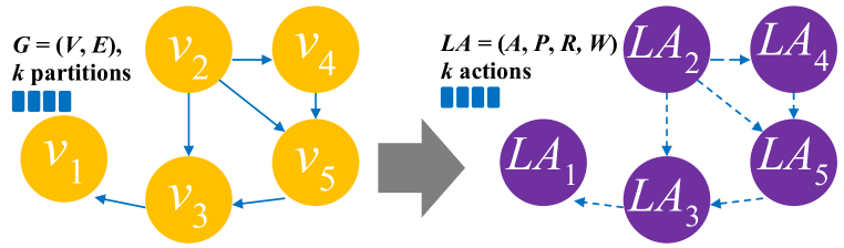
Figure 1: LA with $k$ actions are allocated for nodes of graph. The rectangles represent LA actions associated with partitions.

IV-D How to use label propagation to train a reinforcement learning algorithm

IV-D1 LA action selection

Each step of Revolver starts with LA taking actions for determining the partitions of vertices locally ( in Figure 2). Each vertex has an analogous learning automaton in the network of LA with an action set equal to the available partitions. The LA determines the candidate partition for the vertex using a roulette wheel populated by its probability vector. Actions with larger probabilities will have a higher chance for being selected by the automaton.

IV-D2 Calculating vertex migration probability

After taking actions by LA and selecting candidate partitions for vertices, the remaining load of partition $l$ is calculated using the edges currently assigned to it (i.e., $C-b(l)$) and the demanding load is computed using the number of candidate edges in $l$ (i.e., $\sum_{u\in M(l)}deg(u)$) (see Section III-A). Lastly, to calculate the probability for a vertex to migrate to a candidate partition, we simply divide the remaining load by the demanding load.

IV-D3 Computing vertex score

The normalized LP in (10) is used to calculate a score for each partition of a vertex based on the vertex’s neighboring vertices partitions and the current load of the partition ( in Figure 2). To the contrary of other vertex-centric graph partitioning algorithms like Spinner [25], which migrates a vertex $v$ to the partition with the maximum score, Revolver utilizes a $\lambda$ function to extracts the index of the maximum score for future training of LA i.e. $\lambda(v)=\max_{l\in\{1,...,k\}}{(score(v,l))}$. ( in Figure 2).

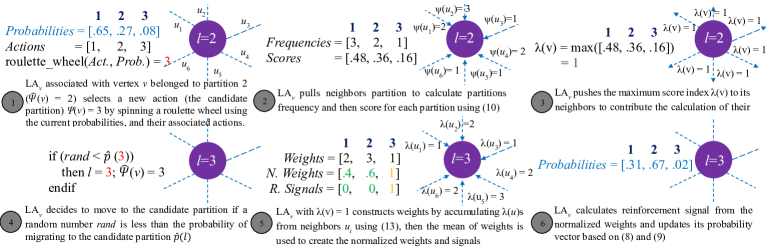
Figure 2: An example of a 3-action learning automaton, $\text{LA}_{v}$, corresponding to vertex $v$, interacting with its neighbors through push and pull mechanisms to partition a graph into 3 sub-partitions. In the beginning of the step, the current label for $v$ is $l=2$ and the probability vector for $\text{LA}_{v}$ is $[.65,.27,.08]$. At the end of the step, node $v$ is assigned to label 3 ($l=3)$ and the probability vector of $\text{LA}_{v}$ is updated and changed to $[.31,.67,.2]$

IV-D4 Executing vertex migration

The decision for migrating a vertex to a new partition is instrumented by comparing the selected action versus the current partition. If the two are not similar, a random number is generated against the migration probability of the candidate partition to determine whether to move the vertex to the new partition or not ( in Figure 2).

IV-D5 Evaluating the objective function

Vertex $v$ receives the maximum score label of its neighbors $\lambda(u)\ |\ \forall u\in N(v)$ and its learning automaton updates its corresponding weight vector as follows ( in Figure 2):

$$w(v,\lambda(v))\mathrel{+}=\begin{cases}\widehat{w}(u,v)\ \ \ \text{if $\delta(\psi(v),\lambda(u))=1$}\\ 1\ \ \ \ \ \ \ \ \ \ \ \text{else if $\widehat{p}(\lambda(v))\ >0$}\end{cases}$$ (13)

where in (13), $w(v,l)$ is the $l^{th}$ element of the weight vector $W$ belogned to vertex $v$, $\psi$ extracts the partition label assigned to vertex $v$ by its learning automaton (i.e., $\psi:A\rightarrow L$ such that $\psi(v)=l$ if LA$(v)$ assigns $l$ to vertex $v$), $\delta$ is the Kronecker delta, and $\widehat{w}$ and $\widehat{p}$ are defined in Section III-A.

In (13), the learning automaton associated with $u\in N(v)$ will receive a reinforcement signal proportional to $w(u,v)$ in two cases: 1) if the selected action of $\text{LA}_{v}$ is equal to $\lambda(v)$, or 2) if the migration probability of the selected action (or partition) $l$ is positive. Hence, these two cases try to reinforce actions associated with the highest score while preserving the balance by taking into account the probability of migration.

IV-D6 Constructing the reinforcement signals

The weight vector $W$ is a vector of weights populated by vertices belonged to $N(v)$. This vector shows the decency of partitions in $N(v)$, where higher weights represent the more promising partitions. To differentiate between favorable and unfavorable partitions while constructing the reinforcement signal $R$, we divide $W$ into two parts using its mean. Specifically, if $w_{i}$ is larger than the mean of weights, $r_{i}=0$ (reward signal); otherwise $r_{i}=1$ (penalty signal) ( in Figure 2).

Lastly, each half of $W$ needs to be normalized independently so as the sum of each half becomes 1 and the sum of weight vector $W$ becomes 2. Normalized weights of reward and penalty reinforcement signals are necessary to keep the sum of LA probabilities equal to 1 while using (8) and (9).

IV-D7 Updating learning automata probability vector

After calculating weights and signals, the probability vector of a vertex $v$ is updated using (8) and (9) ( in Figure 2).

IV-D8 Updating remaining capacity

Calculating the remaining capacity is a simple subtraction of partition capacity $C$ from the current load of partition $b(l)$ at the end of each step.

IV-D9 Checking convergence

Finally, Revolver halts if for a specified number of consecutive steps, score has not improved (i.e., $(S^{i}-S^{i-1})<\theta$, where $\theta$ is the min score difference.)

V Experiments

V-A Experimental Environment

We conducted our experiments on a cluster of 96 nodes (especially that we implemented two versions of Revolver, distributed and parallel ones as noted shortly), each with 64 GB RAM and a 28 cores Intel Xeon CPU E5-2690 running at 2.60 GHz (Broadwell). The operating system of each node is Red Hat Enterprise Linux Server 7.3 (Maipo) with Linux kernel 3.10.0. Communication between nodes is achieved using Intel (R) Omni-Path with channel speed of 100 GB/s.

V-B Datasets

Table I reports the selected graphs along with their numbers of vertices and edges, densities, and skewnesses. In Table I, the density of a graph $G(V,E)$ is calculated using $D=|E|/(|V|\cdot(|V|-1))$, and Pearson’s 1^st skewness coefficient is computed using $(\mu-m)/\sigma$, where $\mu,m,$ and $\sigma$ are the mean, mode, and standard deviation of the outdegree edges. Negative or positive values of density illustrates to what degree a graph is skewed (i.e., whether toward left or right of the outdegree edges). From nine graphs, SO [42] and EU [43] are almost skew-free, USA [44] is uniquely left-skewed, and the rest are right-skewed, whereby they follow a power law distribution. Note that we use different graphs with varied degrees of skewness so as to comprehensively demonstrate the performance of Revolver.

TABLE I: Graph datasets with numbers of Vertices, Edges, Densities ($\times 10^{-5}$), and Pearson’s 1^st skewness coefficients.

Graph	$|V|$	$|E|$	$D$	Skew
Wiki-topcats (WIKI) [42]	1.79M	28.51M	0.88	+0.35
UK-2007@1M (UK) [43]	1.00M	41.24M	4.12	+0.81
USA-road (USA) [44]	23.9M	58.33M	0.01	-0.59
Stackoverflow (SO) [42]	2.60M	63.49M	0.93	+0.08
LiveJournal (LJ) [42]	4.84M	68.99M	0.29	+0.36
EN-wiki-2013 (EN) [43]	4.20M	101.3M	0.57	+0.35
Orkut (OK) [42]	3.07M	117.1M	1.24	+0.29
Hollywood (HLWD) [43]	2.18M	228.9M	4.81	+0.32
EU-2015-host (EU) [43]	11.2M	386.9M	0.30	+0.07

V-C Implementation Details

We implemented two versions of Revolver, a multi-threaded asynchronous one in C/C++ and a synchronous one in Giraph [15]. To encourage reproducibility and extensibility, we made them both open-source. However, we report the results of the asynchronous version for two reasons: 1) Revolver can benefit from incremental changes in partitions offered by the asynchronous computation model during the partitioning process, and 2) Revolver’s C/C++ implementation efficiently balances the vertices among working threads via allocating each subset of vertices to a separate thread. In particular, the vertices, $V$, of every graph are divided into chunks of size $|V|/n$ (with $n$ being the number of threads) and each chunk is assigned a separate thread on a separate core.

V-D Algorithms

We compared Revolver against a number of partitioning algorithms : 1) Spinner [25], a vertex-centric graph partitioning algorithm, which uses an LP scoring function to determine a suitable partition for every vertex $v$, 2) Hash partitioning, where $v\mod k$ is used to hash a vertex with numerical id $v$ to its designated partition, and 3) Range partitioning, where $(v\cdot k)/|V|$ is utilized to map a vertex with id $v$ to its partition.

V-E Performance Metrics

To demonstrate the quality of partitioning, we borrowed two metrics from [25], namely: 1) $Local\ Edges=(\sum_{\forall(u,v)\in E}{\delta(\widehat{\psi}(u),\widehat{\psi}(v)))}/|E|$, which is the number of edges with both ends at the same partition divided by the total number of edges, and 2) $Max\ Normalized\ Load=Max\ Load/Expected\ Load$, where Max Load is the number of edges assigned to the highest loaded partition $\max_{l\in\{1,...,k\}}(b(l))$ (see Section II) and Expected Load is $|E|/k$. Also, we note that $1-Local\ Edges$ is equal to $Edge\ cuts=(\sum_{(u,v)\in E}{1-\delta(\widehat{\psi}(u),\widehat{\psi}(v)}))/|E|$. Clearly, with a set of machines assuming a one-to-one mapping from nodes to partitions, these metrics illustrate the degree at which a given workload can uniformly harness the available computing resources and stress the communication medium at run time. To this end, we indicate that the execution time of the partitioning algorithm as a performance metric is less informative in this context since having a faster runtime does not necessarily lead to better partitions.

Communication becomes a bottleneck if an algorithm requires to perform a massive amount of message passing after each execution step. To this end, the metrics local edges and edge cuts represent the amount of intra-partition and inter-partition interactions, respectively and assess the degree to which an application may require sending/receiving internal or external messages. Furthermore, for an iterative application, the runtime of a single step of execution is bounded by the computation done at the highest loaded machine, which adds up to the latency of the system as well. As such, the metric max normalized load captures the extent to which the computation time is affected by the highest loaded partition.

V-F Experimental Settings

In Figure 3, we report the average local edges and max normalized load for 10 individual runs of each algorithm across different numbers of partitions 2, 4, 8, 16 32, 64, 128, 192, and 256. The results shown for Spinner are collected using Spinner’s original implementation in Giraph [25]. Moreover, for fair comparison, the same parameter settings as in [25] are used to run Revolver and Spinner. Specifically, we set the max number of steps to 290, the max number of consecutive iterations for halting to 5, the min halting score difference to 0.001, and the imbalance ratio $\epsilon$ to 0.05. In addition, the LA reward and penalty parameters $\alpha$ and $\beta$ are set to 1 and 0.1, respectively. We note that the maximum normalized load for Range partitioning is so bad (e.g., Revolver has 60 times improvement compared to Range with 256 partitions on EU graph); hence, we removed it from Figure 3 (except for USA graph) to avoid spoiling the plot scale.

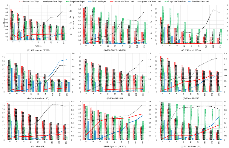
Figure 3: Average local edges (bars scaled according to the left y axis) and max normalized load (lines scaled according to the right y axis) of Revolver, Spinner, Range, and Hash (Range max normalized load is removed intentionally from all charts except USA).

V-G Analysis of Local Edges

We now discuss the results shown in Figure 3. To start with, the clustered bars refer to local edges (left axis) and the lines denote max normalized load (right axis).

V-G1 Right-skewed graphs

WIKI, OK, LJ, EN, and HLWD are right-skewed graphs (see Table I). Compared to Spinner, Hash, and Range, for WIKI (Figure 3-A) and OK (Figure 3-G), Revolver produces the best local edges with 2 - 64 partitions. Furthermore, it achieves the best local edges for LJ (Figure 3-F), while maintaining 5% improvement versus Spinner across all partitions. Alongside, it provides the best local edges for EN (Figure 3-E) with 2 - 16 partitions. Lastly, compared to Spinner and Hash, Revolver produces the best local edges for HLWD (Figure 3-H) with 2 - 128 partitions (almost 5% improvement). In conclusion, Revolver adaptive strategy makes it a decent choice for partitioning right-skewed graphs, especially under smaller numbers of partitions.

V-G2 Highly right-skewed graphs

UK is a highly right-skewed graph. Range produces the best local edges for UK, while Revolver accomplishes better max normalized load on this graph (Figure 3-B). The right skewness feature of UK (Pearson’s first rank = +0.81) indicates that the $mean$ of outdegree edges is far greater than of its $mode$, entailing that most of vertices have degrees less than the $mean$. Range partitions the graph based on the range of vertices and can exploit this UK’s feature. Also, in comparing Revolver against Spinner, Revolver achieves better results with 256 partitions.

V-G3 Skew-free graphs

For skew-free graphs like SO and EU, Revolver produces the best local edges for SO (Figure 3-D) with 4 - 16, 128 - 256 partitions, while Range provides the best local edges for EU (Figure 3-I). Compared to EU, in SO, which is a denser graph with $D=0.93\times 10^{-5}$ (see Table I), Revolver can produce better localized partitions for almost any number of partitions which shows it can effectively partition this type of graphs, independent of the number of partitions.

V-G4 Left-skewed graphs

For left-skewed graphs like USA (Figure 3-C), Range produces better local edges and comparable max normalized load against Revolver. USA is a highly left-skewed graph (Pearson’s first rank = -0.59) (see Table I), which implies that outdegree edges are evenly distributed across vertices. Clearly, Range perfectly benefits from this characteristic and, accordingly, achieves superior results.

V-G5 Impact of graph density and skewness on partitioning

To summarize the results of local edges, Revolver effectively partitioned both right-skewed and skew free graphs because its partitioning strategy is not highly depended to the way edges are distributed among vertices. Range exclusively partitioned highly right-skewed, dense skew free, and highly left-skewed graphs where edges are distributed evenly among vertices. For these kinds of graphs, Range’s partitioning strategy simply extracts partitions from ranges of consecutive vertices while enjoying a balanced distribution of outdegree edges.

V-H Analysis of Max Normalized Load

V-H1 Trade-off between local edges and max normalized load

From Figure 3-A all the way to Figure 3-I (lines), Revolver always produces significantly better max normalized load compared to other algorithms, irrespective of the type of the graph. Unlike Spinner, Revolver’s normalized LP does not allow the penalty function to vary the score independently and, subsequently, create unbalaced partitions. Revolver and Spinner leverage a 5% imbalance ratio ($|E|/k\cdot(1+\epsilon)$, where $\epsilon=0.05$), yet the largest partition produced by Spinner is always bigger than the allowed extra capacity. Evidently, this explains why Spinner accomplishes better local edges (i.e., because larger partitions will have more local edges). On the other hand, Hash produces comparable balanced partitions for these graphs with 2 - 64 partitions, while it always generates the worst local edges. Lastly, although Range provides the best local edges for UK, USA, and EU graphs, it achieves the worst max normalized load among all graphs (e.g., max normalized load of 1.6 - 60 times worst than Revolver for 2 - 256 partitions on EU), except for USA. Range is highly dependant on the way edges are distributed among vertices. The reason for why Range outperforms other algorithms on USA is that USA is a sparse ($D=0.01\times 10^{-5}$) left-skewed graph with edges laid out evenly across vertices.

V-H2 The impact of asynchronous processing

Since Revolver adopts an asynchronous computational model, the process of computing the scores of partitions and migrating a vertex to a new partition is executed on-the-fly, whereby loads of the source and destination partitions are exchanged progressively. This relaxes the migration condition and enables Revolver to attain better max normalized load via utilizing the most recent changes in the partitioning configuration. Compared to Spinner, which is implemented synchronously, the asynchronous model of Revolver has a significant impact on the load distribution as shown in Figure 3-A - Figure 3-I (e.g., up to 28 $\times$ improvement in max normalized load on EU).

V-I The Scalability Feature of Learning Automata

In a partitioning problem, as the number of partitions increases, the complexity of the problem grows as well. This is an inevitable outcome of the curse of dimensionality. In LA, as the number of actions increases, the initial probabilities are decreased which makes it harder to find optimal actions. Our weighted LA (see (8) and (9)) is designed to account for any increase in the dimensionality of the problem by having a weight for each element in the probability vector (which separates probability updates from the space complexity of the problem). Consequently, our weighted updating strategy guarantees a fair distribution of probabilities among the elements of the probability vector. This unique feature makes LA scalable and resistant to increases in the number of partitions.

V-J Convergence Characteristics of Revolver

As Revolver and Spinner have clear advantages over Range and Hash in Sections V-G and V-H, in Figure 4, we draw the convergence characteristics of local edges and max normalized load (left and right y axes) of Revolver and Spinner over LJ with 8 partitions and $\epsilon=0.05$ (other graphs show a similar pattern to Figure 4 and are not shown due to space limitations).

Figure 4 demonstrates an interesting observation about local edges. Specifically, Spinner’s local edges become almost fixed after step 100, while Revolver keeps increasing local edges up to the end (step 300). This clearly indicates the strength of Revolver’s adaptive strategy, which continuously allows reaching a consensus and does not get trapped in a local minimum. On the flip side, the greedy strategy of Spinner gets it trapped early on during execution. Moreover, there is a 5% difference between the local edges produced by Revolver and Spinner, which further illustrates Revolver’s superiority. In addition, Spinner stops increasing local edges when it fully utilizes the 5% extra capacity ($\epsilon=0.05$), while Revolver continues enhancing local edges, even without exhausting the entire available extra capacity.

Comparing local edges and max normalized load, when Revolver hits the plateau of local edges after 30 steps, it harnesses up to 2% extra capacity, whereas, Spinner local edges are only improved when more extra capacity is used (two middle lines of Figure 4 shows this where local edges of Spinner is improved as a function of max normalized load).

Figure 4 also illuminates another pattern. In particular, Spinner tends to utilize its entire extra capacity in the first 75 steps, while Revolver barely consumes up to 2% extra capacity during the whole run. The huge gap between Revolver’s and Spinner’s max normalized load is due to the fact that the asynchronous computation model of Revolver helps LA creating balanced partitions while utilizing significantly less extra capacity. In contrary, Spinner fails in achieving balanced partitions because of its strict synchronous model.

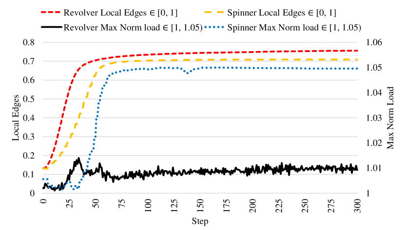
Figure 4: Revolver convergence for LJ with 32 partitions across 290 steps.

VI Conclusions

In this work, we proposed Revolver, an asynchronous reinforcement learning algorithm capable of partitioning multimillion-node graphs. In Revolver, each vertex is assigned to an independent learning automaton to determine the corresponding suitable partition. In addition, a normalized label propagation algorithm is incorporated to asses partitioning results and provide feedback to learning automata. Experimental results show that Revolver can provide locally-preserving partitions, without sacrificing load balance.

VII Acknowledgments

This publication was made possible by NPRP grant #7-1330-2-483 from the Qatar National Research Fund (a member of Qatar Foundation). This research was supported in part by the University of Pittsburgh Center for Research Computing through the resources provided.

References

- [1] Y. Ahmad, O. Khattab, A. Malik, A. Musleh, M. Hammoud, M. Kutlu, M. Shehata, and T. Elsayed, “La3: a scalable link-and locality-aware linear algebra-based graph analytics system,” Proceedings of the VLDB Endowment, vol. 11, no. 8, pp. 920–933, 2018.
- [2] M. Redekopp, Y. Simmhan, and V. K. Prasanna, “Performance analysis of vertex centric graph algorithms on the azure cloud platform,” in Workshop on Parallel Algorithms and Software for Analysis of Massive Graphs. Citeseer, 2011.
- [3] J. E. Gonzalez, Y. Low, H. Gu, D. Bickson, and C. Guestrin, “Powergraph: Distributed graph-parallel computation on natural graphs.” in OSDI, vol. 12, no. 1, 2012, p. 2.
- [4] Amazon.com, Inc. (2018) Amazon elastic compute cloud (amazon ec2). [Online]. Available: https://aws.amazon.com/ec2/
- [5] Microsoft Corporation. (2018) Microsoft azure cloud services. [Online]. Available: https://azure.microsoft.com/
- [6] Google LLC. (2018) Google app engine platfrorm. [Online]. Available: https://cloud.google.com/appengine/
- [7] Y. Wang, A. Davidson, Y. Pan, Y. Wu, A. Riffel, and J. D. Owens, “Gunrock: A high-performance graph processing library on the gpu,” in PPoPP, 2016, p. 11.
- [8] J. Shun and G. E. Blelloch, “Ligra: a lightweight graph processing framework for shared memory,” in ACM Sigplan Notices, vol. 48, no. 8, 2013, pp. 135–146.
- [9] K. Zhang, R. Chen, and H. Chen, “Numa-aware graph-structured analytics,” in ACM SIGPLAN Notices, vol. 50, no. 8, 2015, pp. 183–193.
- [10] D. Nguyen, A. Lenharth, and K. Pingali, “A lightweight infrastructure for graph analytics,” in 24th ACM SOSP, 2013, pp. 456–471.
- [11] A. Kyrola, G. E. Blelloch, C. Guestrin et al., “Graphchi: Large-scale graph computation on just a pc.” in OSDI, vol. 12, 2012, pp. 31–46.
- [12] A. Roy, I. Mihailovic, and W. Zwaenepoel, “X-stream: Edge-centric graph processing using streaming partitions,” in SOSP, 2013, p. 472.
- [13] X. Zhu, W. Han, and W. Chen, “Gridgraph: Large-scale graph processing on a single machine using 2-level hierarchical partitioning.” in USENIX Annual Technical Conference, 2015, pp. 375–386.
- [14] S. Maass, C. Min, S. Kashyap, W. Kang, M. Kumar, and T. Kim, “Mosaic: Processing a trillion-edge graph on a single machine,” in 12th ACM EuroSys, 2017, pp. 527–543.
- [15] A. Ching, S. Edunov, M. Kabiljo, D. Logothetis, and S. Muthukrishnan, “One trillion edges: Graph processing at facebook-scale,” Proceedings of the VLDB Endowment, vol. 8, no. 12, pp. 1804–1815, 2015.
- [16] G. Malewicz, M. H. Austern, A. J. Bik, J. C. Dehnert, I. Horn, N. Leiser, and G. Czajkowski, “Pregel: a system for large-scale graph processing,” in 2010 ACM SIGMOD International Conference on Management of data, 2010, pp. 135–146.
- [17] Y. Low, D. Bickson, J. Gonzalez, C. Guestrin, A. Kyrola, and J. M. Hellerstein, “Distributed graphlab: a framework for machine learning and data mining in the cloud,” Proceedings of the VLDB Endowment, vol. 5, no. 8, pp. 716–727, 2012.
- [18] R. Chen, J. Shi, Y. Chen, and H. Chen, “Powerlyra: Differentiated graph computation and partitioning on skewed graphs,” in 10th EuroSys, 2015.
- [19] C. Xie, R. Chen, H. Guan, B. Zang, and H. Chen, “Sync or async: Time to fuse for distributed graph-parallel computation,” ACM SIGPLAN Notices, vol. 50, no. 8, pp. 194–204, 2015.
- [20] Y. Simmhan, A. Kumbhare, C. Wickramaarachchi, S. Nagarkar, S. Ravi, C. Raghavendra, and V. Prasanna, “Goffish: A sub-graph centric framework for large-scale graph analytics,” in European Conference on Parallel Processing. Springer, 2014, pp. 451–462.
- [21] Y. Tian, A. Balmin, S. A. Corsten, S. Tatikonda, and J. McPherson, “From think like a vertex to think like a graph,” Proceedings of the VLDB Endowment, vol. 7, no. 3, pp. 193–204, 2013.
- [22] M. Hammoud and M. F. Sakr, “Distributed programming for the cloud: Models, challenges, and analytics engines.” 2014.
- [23] F. Rahimian, A. H. Payberah, S. Girdzijauskas, M. Jelasity, and S. Haridi, “Ja-be-ja: A distributed algorithm for balanced graph partitioning,” in 7th IEEE SASO, 2013, pp. 51–60.
- [24] C. Tsourakakis, C. Gkantsidis, B. Radunovic, and M. Vojnovic, “Fennel: Streaming graph partitioning for massive scale graphs,” in 7th ACM WSDM, 2014, pp. 333–342.
- [25] C. Martella, D. Logothetis, A. Loukas, and G. Siganos, “Spinner: Scalable graph partitioning in the cloud,” in ICDE, 2017, p. 1083.
- [26] L. G. Valiant, “A bridging model for parallel computation,” Communications of the ACM, vol. 33, no. 8, pp. 103–111, 1990.
- [27] M. J. Barber and J. W. Clark, “Detecting network communities by propagating labels under constraints,” Physical Review E, vol. 80, 2009.
- [28] K. S. Narendra and M. A. Thathachar, Learning automata: an introduction. Courier Corporation, 2012.
- [29] M. Hasanzadeh, M. R. Meybodi, and M. M. Ebadzadeh, “Adaptive cooperative particle swarm optimizer,” Applied Intelligence, vol. 39, no. 2, pp. 397–420, 2013.
- [30] M. Hasanzadeh and M. R. Meybodi, “Grid resource discovery based on distributed learning automata,” Computing, vol. 96, pp. 909–922, 2014.
- [31] M. Hasanzadeh and M. R. Meybodi, “Distributed optimization grid resource discovery,” The Journal of Supercomputing, vol. 71, no. 1, pp. 87–120, 2015.
- [32] A. Jobava, A. Yazidi, B. J. Oommen, and K. Begnum, “On achieving intelligent traffic-aware consolidation of virtual machines in a data center using learning automata,” Journal of Computational Science, vol. 24, pp. 290–312, 2018.
- [33] A. Rezvanian and M. R. Meybodi, “A new learning automata based sampling algorithm for social networks,” International Journal of Communication Systems, vol. 30, no. 5, pp. 1–21, 2017.
- [34] M. H. Mofrad, S. Sadeghi, A. Rezvanian, and M. R. Meybodi, “Cellular edge detection: Combining cellular automata and cellular learning automata,” AEU-International Journal of Electronics and Communications, vol. 69, no. 9, pp. 1282–1290, 2015.
- [35] M. Hasanzadeh-Mofrad and A. Rezvanian, “Learning automata clustering,” Journal of Computational Science, vol. 24, pp. 379–388, 2018.
- [36] B. W. Kernighan and S. Lin, “An efficient heuristic procedure for partitioning graphs,” The Bell system technical journal, vol. 49, no. 2, pp. 291–307, 1970.
- [37] P. K. Chan, M. D. Schlag, and J. Y. Zien, “Spectral k-way ratio-cut partitioning and clustering,” ransactions on computer-aided design of integrated circuits and systems, vol. 13, no. 9, pp. 1088–1096, 1994.
- [38] G. Karypis and V. Kumar, “A fast and high quality multilevel scheme for partitioning irregular graphs,” SIAM Journal on scientific Computing, vol. 20, no. 1, pp. 359–392, 1998.
- [39] U. N. Raghavan, R. Albert, and S. Kumara, “Near linear time algorithm to detect community structures in large-scale networks,” Physical review E, vol. 76, no. 3, p. 036106, 2007.
- [40] D. E. Goldberg, “Probability matching, the magnitude of reinforcement, and classifier system bidding,” Machine Learning, vol. 5, no. 4, pp. 407–425, 1990.
- [41] M. H. Mofrad, R. Melhem, and M. Hammoud, “Revolver: vertex-centric graph partitioning using reinforcement learning,” in 2018 IEEE 11th International Conference on Cloud Computing (CLOUD). IEEE, 2018, pp. 818–821.
- [42] J. Leskovec and A. Krevl, “SNAP Datasets: Stanford large network dataset collection,” http://snap.stanford.edu/data.
- [43] P. Boldi and S. Vigna, “The webgraph framework i: Compression techniques,” in 13th ACM WWW, 2004, pp. 595–601.
- [44] C. Demetrescu, A. V. Goldberg, and D. S. Johnson, “9th DIMACS implementation challenge,” http://www.diag.uniroma1.it/challenge9/.