Magnification, dust and time-delay constraints from the first resolved strongly lensed Type Ia supernova iPTF16geu

Abstract

We report lensing magnifications, extinction, and time-delay estimates for the first resolved, multiply-imaged Type Ia supernova iPTF16geu, at $z=0.409$, using Hubble Space Telescope ($HST$) observations in combination with supporting ground-based data. Multi-band photometry of the resolved images provides unique information about the differential dimming due to dust in the lensing galaxy. Using $HST$ and Keck AO reference images taken after the SN faded, we obtain a total lensing magnification for iPTF16geu of $\mu=67.8^{+2.6}_{-2.9}$, accounting for extinction in the host and lensing galaxy. As expected from the symmetry of the system, we measure very short time-delays for the three fainter images with respect to the brightest one: -0.23 $\pm$ 0.99, -1.43 $\pm$ 0.74 and 1.36 $\pm$ 1.07 days. Interestingly, we find large differences between the magnifications of the four supernova images, even after accounting for uncertainties in the extinction corrections: $\Delta m_{1}=-3.88^{+0.07}_{-0.06}$, $\Delta m_{2}=-2.99^{+0.09}_{-0.08}$, $\Delta m_{3}=-2.19^{+0.14}_{-0.15}$ and $\Delta m_{4}=-2.40^{+0.14}_{-0.12}$ mag, discrepant with model predictions suggesting similar image brightnesses. A possible explanation for the large differences is gravitational lensing by substructures, micro- or millilensing, in addition to the large scale lens causing the image separations. We find that the inferred magnification is insensitive to the assumptions about the dust properties in the host and lens galaxy.

1 Introduction

The discovery of the first multiply-imaged gravitationally lensed Type Ia supernova (SN Ia), iPTF16geu (Goobar et al., 2017, hereafter G17) was a major breakthrough for time-domain astronomy, highlighting the power of wide-field surveys to detect rare phenomena. Transient astrophysical sources that are strongly lensed by foreground galaxies or galaxy clusters are powerful probes in cosmology since they make it possible to measure time delays between the multiple images. More than half a century has passed since Refsdal (1964) proposed that time-delays between multiple images of transients like supernovae (SNe) are useful since they depend sensitively on cosmological parameters, e.g. the Hubble constant ($H_{0}$). The observations also allow us to probe the distribution of matter in the lens. Hence, multiply-resolved gravitationally lensed supernovae (glSNe) are exquisite laboratories for fundamental physics, as well as astrophysical properties of the host and lens galaxies (see Oguri, 2019, for a review of strongly lensing of SNe and other explosive transients). Although strongly lensed galaxies and quasars are more common than glSNe, glSNe have notable advantages, particularly if they are of Type Ia (glSNe Ia). This is because the “standard candle" nature of the SNe Ia allows us to directly measure the magnification factor, which helps us to overcome various degeneracies in estimating $H_{0}$ from strongly lensed transients, including the mass-sheet degeneracy (Falco et al., 1985; Schneider & Sluse, 2014). Additionally, SNe Ia have a well-studied family of light curves and hence, can be used for an accurate measurement of time-delays, with significantly fewer follow-up observations than quasars. Moreover, since SNe fade away, we can obtain post-explosion imaging to validate the lens model.

However, discovering these rare events has proven very challenging and it is only thanks to the recent developments in time domain astronomy that the first lensed supernovae have been detected. Quimby et al. (2013) found a strongly lensed SN Ia but multiple images were not resolved. However, the magnification allowed for high signal to noise spectroscopy at $z>1$ and hence, the SN was used to show that the spectral properties of high-$z$ and nearby SNe Ia are very similar (Petrushevska et al., 2017). The first resolved lensed supernova, SN Refsdal (Kelly et al., 2015), detected with the Hubble Space Telescope ($HST$), is a core-collapse SN magnified by a cluster of galaxies, which makes the lens modelling challenging (Grillo et al., 2018).

The discovery of iPTF16geu showed that glSNe Ia can be found without the need of highly spatially resolved observations, thanks to their "standard candle" nature. At $z=0.409$, the SN was found to be 30 standard deviations too bright compared with the SN Ia population, which prompted us to observe the system from space with $HST$ and with laser guide star adaptive optics (LGS-AO) at VLT and Keck. Here we report on the multi-wavelength follow-up observations carried out while the SN was active in late 2016, as well as laser aided AO Near IR observations with Keck and $HST$ observations after the SN had faded below the detection limit. We use the multi-wavelength light curves from the resolved images in combination with unresolved, ground-based data to constrain the magnifications of the individual SN images (and hence, the total SN magnification) after accounting for the extinction in the different lines of sight to the multiple images.

The accurate SN image positions are used to model the lens, as described in an accompanying paper (Mörtsell et al, in prep). Unlike the case of strongly lensed quasars, as the transient faded, we had an opportunity to verify the lensing model with the reconstruction of the distorted host galaxy image. We compared the model predictions of the flux ratios (based only on the image positions) to the observed value after extinction correction for each image. We used this to assess the possibility that otherwise unaccounted for residuals are caused due to lensing by substructures within the lensing galaxy, in the form of field stars. In another accompanying paper (Johansson et al, in prep) we present the spectroscopic observations of iPTF16geu.

The structure of this paper is as follows. We present the observations of iPTF16geu in Section 2 and the photometric analysis method in Section 3. In Section 4, we describe the multiple-image SN model and the resulting lensing magnification, time-delays and constraints on extinction properties in Section 5. We present the observed magnifications in context of model predictions and discuss the possibility of substructures in Section 6 and discuss observations of future strongly lensed SNe in Section 7. Finally, we present our conclusions in Section 8.

2 Observations

2.1 Hubble Space Telescope Wide Field Camera 3

We observed iPTF16geu with the Hubble Space Telescope ($HST$) Wide Field Camera 3 (WFC3) under programs DD 14862 and GO 15276 (PI: A. Goobar) using the ultra violet (WFC3/UVIS) and near-IR (WFC3/IR) channels. For both channels we only read out part, $512\times 512$ pixels, of the full detectors. However, given the different pixel scales of the two channels, $0.04^{\prime\prime}$/pixel and $0.12^{\prime\prime}$/pixel for WFC3/UVIS and WFC3/IR, respectively, they will not cover the same area on the sky. The data were obtained using either a 3- or 4-point standard dithering pattern for both channels. For WFC3/UVIS we used the UVIS2-C512C-SUB, that is located next to the amplifier, with a post-flash to maximize the charge transfer efficiency (CTE) during read-out. All imaging data are shown in Table 1.

Table 1: Hubble Space Telescope Wide Field Camera 3 data imaging data presented here. The columns are the civil date, the Modified Julian Date (MJD), the $HST$ passband, total exposure time, the number of sub-exposures, and the WFC3 camera. The WFC3/UVIS and WFC3/IR data were obtained with the UVIS2-C512C-SUB and IRSUB512 subarray, respectively.

Civil date	MJD	Filter	Exp.	Sub	Camera
2016-10-20	57681.62	$F475W$	378.0	3	UVIS2
2016-10-20	57681.62	$F625W$	291.0	3	UVIS2
2016-10-20	57681.63	$F814W$	312.0	3	UVIS2
2016-10-20	57681.64	$F110W$	63.9	3	IR
2016-10-20	57681.64	$F160W$	621.4	3	IR
2016-10-25	57685.91	$F625W$	198.0	3	UVIS2
2016-10-25	57685.92	$F814W$	114.0	3	UVIS2
2016-10-25	57685.93	$F475W$	183.0	3	UVIS2
2016-10-25	57685.94	$F390W$	429.0	3	UVIS2
2016-10-25	57685.99	$F110W$	63.9	3	IR
2016-10-25	57685.99	$F160W$	415.1	3	IR
2016-10-29	57689.89	$F475W$	378.0	3	UVIS2
2016-10-29	57689.91	$F625W$	291.0	3	UVIS2
2016-10-29	57689.91	$F814W$	312.0	3	UVIS2
2016-10-29	57689.96	$F110W$	63.9	3	IR
2016-10-29	57689.96	$F160W$	621.4	3	IR
2016-11-02	57694.21	$F625W$	804.0	4	UVIS2
2016-11-02	57694.21	$F814W$	480.0	4	UVIS2
2016-11-02	57694.24	$F110W$	63.9	3	IR
2016-11-02	57694.24	$F160W$	415.1	3	IR
2016-11-02	57694.28	$F105W$	309.4	3	IR
2016-11-06	57698.25	$F625W$	644.0	4	UVIS2
2016-11-06	57698.25	$F814W$	420.0	4	UVIS2
2016-11-06	57698.26	$F110W$	63.9	3	IR
2016-11-06	57698.26	$F160W$	621.4	3	IR
2016-11-10	57702.16	$F625W$	804.0	4	UVIS2
2016-11-10	57702.16	$F814W$	480.0	4	UVIS2
2016-11-10	57702.17	$F110W$	63.9	3	IR
2016-11-10	57702.17	$F160W$	415.1	3	IR
2016-11-15	57707.12	$F625W$	644.0	4	UVIS2
2016-11-15	57707.12	$F814W$	420.0	4	UVIS2
2016-11-15	57707.14	$F110W$	63.9	3	IR
2016-11-15	57707.14	$F160W$	621.4	3	IR
2016-11-17	57709.72	$F625W$	804.0	4	UVIS2
2016-11-17	57709.74	$F814W$	480.0	4	UVIS2
2016-11-17	57709.78	$F110W$	63.9	3	IR
2016-11-17	57709.78	$F160W$	415.1	3	IR
2016-11-22	57714.32	$F625W$	644.0	4	UVIS2
2016-11-22	57714.32	$F814W$	420.0	4	UVIS2
2016-11-22	57714.35	$F110W$	63.9	3	IR
2016-11-22	57714.35	$F160W$	621.4	3	IR
2018-11-10	58432.37	$F390W$	1454.0	4	UVIS2
2018-11-10	58432.38	$F475W$	1494.0	4	UVIS2
2018-11-10	58432.40	$F814W$	1227.0	4	UVIS2
2018-11-10	58432.40	$F625W$	1648.0	4	UVIS2
2018-11-10	58432.48	$F110W$	125.3	3	IR
2018-11-10	58432.48	$F105W$	483.9	3	IR
2018-11-10	58432.48	$F160W$	965.3	3	IR

We used the automatic calwf3 reduction pipeline at the Space Telescope Science Institute, on all the data to dark subtract, flat-field and correct the data for charge-transfer inefficiency. The individual images were then combined and corrected for geometric distortion using the AstroDrizzle software.

2.2 Ground data

In addition to the data already presented in G17, iPTF16geu was observed from the ground until it disappeared behind the Sun. We obtained laser guided adaptive optics (LGS-AO) observations with NIRC2 at the Keck II telescope on Mauna Kea in J, H and $K_{S}$ bands on UTC 2017, June, 16, after iPTF16geu had faded. For the J and H bands we obtained 9 exposures in a dithering pattern, each with an integration time of 20 s. For the $K_{S}$ band, 18 exposures of 65 s were acquired.

Standard near infrared reduction was applied where the individual images were first dark subtracted and flat fielded. The flat frames were obtained using the same dome on-off technique as described in G17. The sky background for each science frame was obtained from the images preceding and following each exposure, after first masking out the object. Together with data presented in G17 this resulted in a total of 3 epochs for the NIRC2/J and 2 epochs for the NIRC2/H and NIRC2/Ks bands, respectively.

We also obtained $rizYJH$ photometry of iPTF16geu with the multi-channel Reionization And Transients InfraRed camera (RATIR; Butler et al., 2012) mounted on the 1.5-m Johnson telescope at the Mexican Observatorio Astronomico Nacional on Sierra San Pedro Martir (SPM) in Baja California, Mexico (Watson et al., 2012). The RATIR data were reduced and coadded using standard CCD and IR processing techniques in IDL and Python, utilizing the online astrometry programs SExtractor and SWarp. Calibration was performed using field stars with reported fluxes in both 2MASS (Skrutskie et al., 2006) and the SDSS Data Release 9 Catalogue (Ahn et al., 2012).

3 Photometric analysis

In this section we detail the analysis methodology to obtain multiband WFC3 photometry for the resolved images. In section 3.1 we detail the procedure to forward model the NIRC2 LGS-AO images. We derive the WFC3 photometry using two different approaches. The forward modelling approach is described in section 3.2 and the template subtractions in section 3.3. We measure the fluxes for all the SN images simultaneously. For our analyses, we use the template subtracted photometry since this approach is independent of the assumptions on the host and lens galaxy models.

3.1 Forward modelling of the NIRC2 images

The LGS-AO NIRC2 images have the highest spatial resolution in our data set. We use the NIRC2 data to build a parametric model of the iPTF16geu system, including the SN images, the host galaxy, and the lens. The model we use is described in detail in §A, and is only briefly summarized here. The shape of the lensing galaxy is modeled with a Sérsic profile (Sérsic, 1963) while the SN images are modeled by the point-spread function (PSF) of the images, assumed to be a Moffat profile. The shape of the SN host galaxy is described by the expansion in eq. (3). The full model is then fitted simultaneously to all data in one NIRC2 filter at a time. Some parameters, such as the host and lens models and the position of the SN images, are forced to be the same for all available images in a filter, while the fluxes of the SN images are allowed to vary between the different epochs, with the exception of the reference images obtained in 2017 where all SN fluxes are fixed to zero, which breaks the degeneracy between the PSFs and the background model.

Examples of data and the fitted models are shown in Figure 1. The fitted positions of the four SN images for the NIRC2 J-band are further presented Table 4, while the lens and host parameters are shown in Tables 5–2. We use the J-band as the reference since the ratio between the SN flux and background is the highest of all NIRC2 filters and we have two epochs where the SN is active.

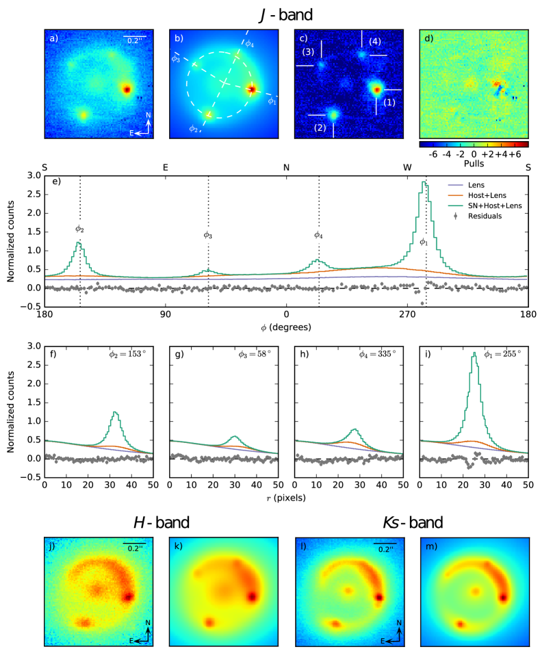
Figure 1: a) NIRC2 J image of the iPTF16geu system obtained on on Nov 5, 2016. b) The model fitted simultaneously to all available epochs as described in the text. The dashed circle shows the position of the host galaxy as described in eq. (5). The dashed lines are showing the angular positions of the four SN images. c) The subtraction between the data and the host and lens models. The fitted PSF positions of the four SN images have been marked. d) The ”pulls”, i.e. the residuals normalized with the pixel uncertainties when the lens, host and SN model is subtracted from the data. e) The profile of both the model and the residuals along the host radius marked by the dashed circle in b), The fitted angles, $\phi_{i}$, of the SN images are marked by the dotted, black lines. f) – i) The radial profiles from the center for the SN images as marked and labelled in b). j) – k) NIRC2 H image obtained on Oct 23, 2016 and the corresponding fitted model. l) – m) NIRC2 Ks image obtained on Oct 22, 2016 and the corresponding fitted model.

Table 2: The fitted widths, $\sigma_{H}$, for the host model defined in eq. (3).

Filter	$\sigma_{H}$
	$(^{\prime\prime})$
$K_{s}$	0.080	(0.001)
$H$	0.129	(0.001)
$F160W$	∗0.129
$J$	0.102	(0.003)
$F110W$	∗0.102
$F814W$	0.067	(0.002)
$F625W$	0.056	(0.003)
$F475W$	∗0.056

As seen in Figure 1, the model generally fits the data well. Four SN images are clearly visible in the J-band but from panel d) we also see that the fit is not perfect. Discrepancies can mainly be seen for the brightest SN image, which are probably due to an imperfect PSF model, rather than an insufficient background model. In other words, if the systematic PSF uncertainties are known, the method can be used to obtain fluxes for the four SN images.

From the radial profile plots in panels f)–i) there is an apparent degeneracy between the host model and the SN profiles given that their extrema coincide and have similar width. However, recall that we only fit one parameter, $\sigma_{H}$, for the width of the host model, as explained in §A, and the value of this parameter will mainly be determined by the pixels between the images located along the dashed circle in panel b). Furthermore, by studying the profile along this circle, as shown in panel e), we can conclude that the maximum of the host galaxy amplitude appears to be located between images (1) and (4), and the best fit model suggest that the background flux under the SN images is either increasing or decreasing monotonically.

Since the image positions are not expected to change with time or wavelength, we fixed the positions to the values in Table 4 for the remaining of the analysis in this paper.

With the SN positions fixed we move on to fit the host model for the remaining NIRC2 filters. The fitted models to the H- and Ks-band are shown in panels j)–m) in Figure 1. In the figure, the epochs when the SN was active are shown together with the corresponding data. The lens and host model parameters are presented in Tables 5–2.

Note that in this paper, we number the Images 1 $\rightarrow$ 4 clockwise from the brightest image (middle right in the data presented in Figure 1 Panel c))

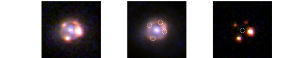
Figure 2: $HST$ observations from 2016, October, 29, in a combination of $F814W$, $F625W$, $F475W$ filters of iPTF16geu (left), post-explosion template (middle) and the subtracted image (right)

3.2 WFC3 photometry using forward modelling

Here we describe the WFC3 photometry computed using the forward modelling approach. We emphasize that this procedure was only used to extract fluxes before the images after the SN faded were obtained. The photometry estimated using this method is not used in any of the analyses described below. We use the same approach detailed in §3.1 to extract the SN photometry. Details of the fitting procedure are described in § B and the fitted parameters presented in Tables 5–2.

Below we describe the procedure to build lightcurves from template subtracted images. Since we see that there are some significant residuals in panel d) of Figure 1 and that the template subtraction approach is significantly more model independent, we use the resulting SN fluxes from the template subtractions in our analyses.

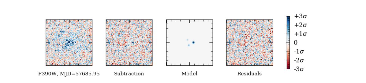
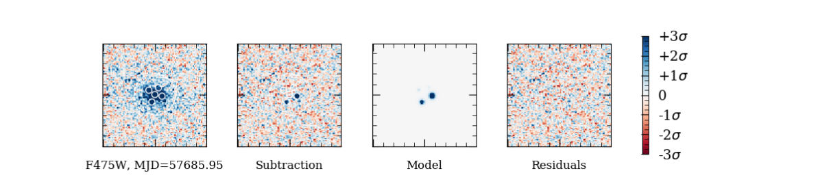
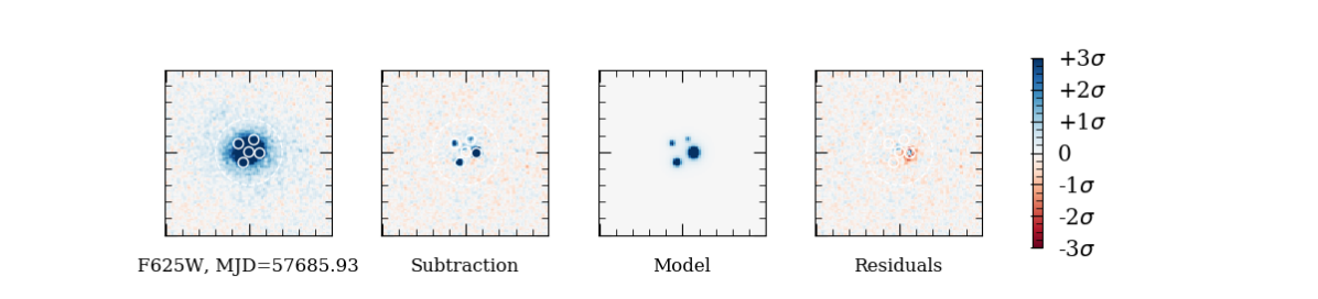
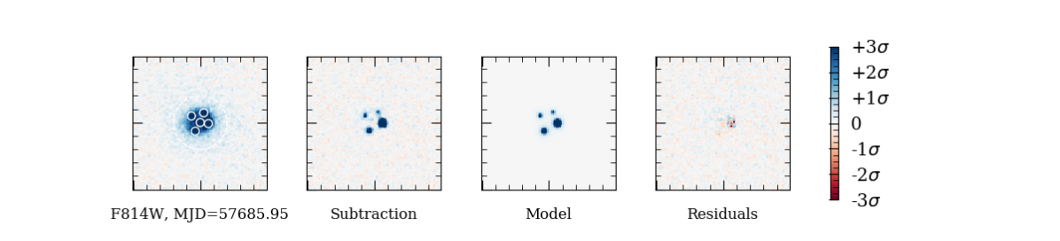
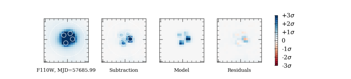
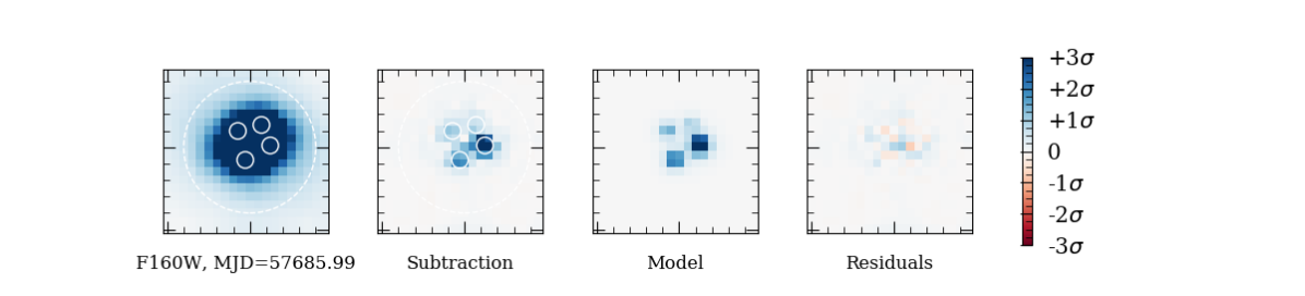
Figure 3: $HST$ observations taken on 2016 October 20 in the $F390W$, $F475W$, $F625W$, $F814W$, $F110W$, $F160W$ filters, together with template subtracted images, fitted PSF models and residuals after the four SN PSFs have been subtracted, for each filter.

Table 3: This table summarises the resulting best fit parameters by fitting an sncosmo model to the ground-based and HST observations (equation 1). For each image, we present the time of maximum, t_max (relative to image 1), host galaxy colour excess (which is treated as being the same for each image), the lens galaxy colour excess as well as the magnification for each image (given as the 68$\%$ credible region of the posterior distribution). Our fiducial case assumes $R_{V}=2$ in both the host and the lens galaxy. We also present the parameters values assuming host $R_{V}=2$ and lens $R_{V}$ as a free parameters as well as the case with host and lens $R_{V}$ fixed to the Milky Way value of 3.1.

Parameter	Image 1	Image 2	Image 3	Image 4
Fiducial fit parameters:
(fixed $R_{V}^{\rm lens}\equiv 2$, fixed $R_{V}^{\rm host}\equiv 2$)
$t_{\rm max}$	57652.80 ($\pm$ 0.33)	-0.23 ($\pm$ 0.99)	-1.43 ($\pm$ 0.74)	1.36 ($\pm$ 1.07)
Stretch, $s$	0.99 ($\pm$ 0.01)	Same as Image 1	Same as Image 1	Same as Image 1
$E(B-V)_{\rm host}$	0.29 ($\pm$ 0.05)	Same as Image 1	Same as Image 1	Same as Image 1
$E(B-V)_{\rm lens}$	0.06 ($\pm$ 0.08)	0.17 ($\pm$ 0.08)	0.42 ($\pm$ 0.09)	0.94 ($\pm$ 0.07)
Magnification	$-3.88^{+0.07}_{-0.06}$	$-2.99^{+0.09}_{-0.08}$	$-2.19^{+0.14}_{-0.15}$	$-2.40^{+0.14}_{-0.12}$
Reddening assumptions modified:
(free $R_{V}^{\rm lens}$, fixed $R_{V}^{\rm host}\equiv 2$)
$t_{\rm max}$	57652.9 ($\pm$ 0.20)	-0.31 ($\pm$ 0.93)	-1.84 ($\pm$ 0.90)	0.77 ($\pm$ 1.27)
Stretch, $s$	1.00 ($\pm$ 0.01)	Same as Image 1	Same as Image 1	Same as Image 1
$E(B-V)_{\rm host}$	0.18 ($\pm$ 0.05)	Same as Image 1	Same as Image 1	Same as Image 1
$E(B-V)_{\rm lens}$	0.26 ($\pm$ 0.09)	0.41 ($\pm$ 0.10)	0.78 ($\pm$ 0.12)	1.58 ($\pm$ 0.14)
$R_{V}^{\rm lens}$ (single $R_{V}$)	$<1.8$	Same as Image 1	Same as Image 1	Same as Image 1
$R_{V}^{\rm lens}$ (all free)	$<2.8$	$<3.2$	$<3.6$	$<1.5$
Magnification	$-3.78^{+0.09}_{-0.10}$	$-2.85^{+0.10}_{-0.11}$	$-1.86^{+0.15}_{-0.15}$	$-1.98^{+0.16}_{-0.17}$
($R_{V}^{\rm lens}\equiv 3.1$, $R_{V}^{\rm host}\equiv 3.1$)
$t_{\rm max}$	57652.7 ($\pm$ 0.38)	0.11 ($\pm$ 0.91)	-0.85 ($\pm$ 1.08)	-0.41 ($\pm$ 2.27)
Stretch, $s$	1.01 ($\pm$ 0.01)	Same as Image 1	Same as Image 1	Same as Image 1
$E(B-V)_{\rm host}$	0.17 ($\pm$ 0.08)	Same as Image 1	Same as Image 1	Same as Image 1
$E(B-V)_{\rm lens}$	0.13 ($\pm$ 0.08)	0.20 ($\pm$ 0.09)	0.40 ($\pm$ 0.09)	0.70 ($\pm$ 0.09)
Magnification	$-4.04^{+0.12}_{-0.08}$	$-3.18^{+0.14}_{-0.13}$	$-2.39^{+0.22}_{-0.23}$	$-2.57^{+0.11}_{-0.07}$

3.3 WFC3 photometry from subtracted images

On 2018 November 10, we obtained $HST$ WFC3 images of the lens and host galaxy system, long after the SN faded. This allowed us to align the SN images and the template images and subtract the lens and host galaxy contribution (see Figure 2 for the combined RGB image, the template and the subtraction). This approach is freed from the assumptions of host and lens galaxy modeling. We note, however, that the challenge of lack of field stars and PSF sampling still remains.

On the subtracted images, we use four Moffat PSF models to simultaneously fit the SN images. The relative SN image positions are kept fixed. The errors are estimated by randomly putting small apertures on the residual image. For Images 1 and 2, the forward modelling (Sections 3.2 and Appendix B) and template subtraction have very good agreement within the statistical errors. However, since Images 3 and 4 are significantly fainter, there are systematic differences in the template subtractions and the forward modelling. Examples of the SN data for 2016, October, 20, subtraction, model and residuals for all the WFC3 filters is shown in Figure 3. Since this approach is significantly less model dependent, we use this version of the photometry in the analysis detailed below. The photometry is presented in section C.

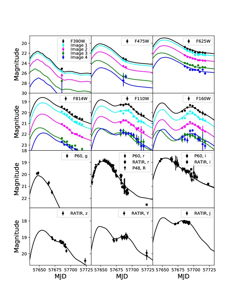
Figure 4: The multiple image model fit to the resolved photometry for the individual images from $HST$ (top six panels). The $HST$ data for Image 1 is in cyan, Image 2 in magenta, Image 3 in green and Image 4 in blue. The black lines show the combined data. The combined fit to the ground based data where the multiple images are not resolved (bottom six panels). The filters are plotted in ascending order of effective wavelength. The RATIR, Y data are scaled down by 0.25 mag to account for unknown systematic effects.

4 Lightcurve fitting model

In this section we present the model to fit the light curves of iPTF16geu. We combine the ground based data with the resolved photometry from $HST$ to fit for the global lightcurve parameters: lightcurve shape (or stretch, $s$), color excess from either intrinsic color variations or dimming by dust in the host galaxy. In addition, we use the multi-band lightcurves of the resolved SN images to fit for the lightcurve peaks and time offsets between the four SN images, as well as extinction in the lensing galaxy for each individual line of sight. Here, we describe the SN model constructed to derive the time-delay, magnification and extinction parameters for iPTF16geu.. We construct a multiple-image model for an SN Ia using sncosmo (Barbary et al., 2016) with a Hsiao model for the SN Ia spectral template, which is constructed from a large library of spectra for diverse SNe Ia. The Hsiao model is appropriate since iPTF16geu shows light curve and spectroscopic properties consistent with normal SNe Ia. SNe Ia in the local universe show a characteristic near infrared (NIR; $iYJHK$) light curve morphology (Hamuy et al., 1996; Folatelli et al., 2010). Unlike in the optical, where the light curves decline after peak, in the NIR, SNe Ia rebrighten 2-3 weeks after the $B$-band maximum. This feature has also been seen in well-studied intermediate-$z$ SNe (e.g., see Riess et al., 2000). iPTF16geu shows a distinct second maxmium in the observer frame F110W and F160W filters. Accounting for time-dilation and K-correction, we find that the time of the second maximum ($t_{2}$) 29.3 $\pm$ 1.1 days after $B$-band maximum, consistent with the median value of $t_{2}$ for nearby, normal, SNe Ia (Biscardi et al., 2012; Dhawan et al., 2015). Since $t_{2}$ only depends on the redshift but not the distance, this further justifies the choice of using a normal SN Ia model to fit the iPTF16geu light curves.

We also correct the light curves for Milky Way (MW) dust. For all our dust corrections, we use the Milky Way reddening law (Cardelli et al., 1989, hereafter CCM89). In our fiducial analysis, we fix the $R_{V}$, for the CCM89 dust correction, to 2 in the host and lens galaxies and to the canonical value of 3.1 in the Milky Way. The value of host and lens galaxy $R_{V}$ is chosen from the slope of the luminosity-colour relation ($\beta\sim 3$, hence, $R_{V}\sim 2$) from the most updated cosmological samples of SNe Ia (see; Scolnic et al., 2018; DES Collaboration et al., 2018). Since iPTF16geu shows light curve and spectroscopic features similar to core-normal SNe Ia (Cano et al., 2018, Johansson et al. in prep), which are used for constraining cosmology, we can use the mean $R_{V}$ from the cosmological compilations when fitting for the light curve model parameters for iPTF16geu. Hence, in our model fit, we include the following parameters

• The stretch, $s$, for the SN

• The colour excess, $E(B-V)$ in the host galaxy

• The colour excess, $E(B-V)$ for the individual images in the lens galaxy

• The time of maximum $t_{\rm max}$ for each of the four images, and hence, the time-delays between the images

• The magnification for each of the four images

$$\chi^{2} =\sum_{\lambda}^{\mathrm{Ground}}\frac{\left[\left(\sum_{i}^{N}{\rm F}_{i}^{\rm model}(t,\lambda)\right)-{\rm F}^{\rm data}(t,\lambda)\right]^{2}}{\sigma^{2}(t,\lambda)}+$$ (1)

$$\quad\sum_{\lambda}^{\mathrm{HST}}\sum_{i}^{N}\frac{\left[{\rm F}_{i}^{\rm model}(t,\lambda)-{\rm F}_{i}^{\rm data}(t,\lambda)\right]^{2}}{\sigma_{i}^{2}(t,\lambda)},$$

We fit the model to the observations using a $\chi^{2}$ likelihood with two terms for the ground based and the $HST$ data. For the ground based data we compare the sum of the models to the observations, whereas for the $HST$ data we compare the individual images, where $F$ is the flux, $t$ is the epoch of the SN Ia light curve, $N$ is the number of images and $\lambda$ is the effective wavelength of each filter. The model is fitted using a nested sampling software nestle implemented in sncosmo.

5 Results

In this section, we present the results of fitting the multiple-image SN model described in Section 4 to the observations of iPTF16geu (see Figure 4). In our analyses, we add an additional error term corresponding to 8$\%$ of the flux to the diagonal terms of the error covariance matrix for the $HST$ observations such that the reduced $\chi^{2}$ for the ground and space-based data individually (and hence, the total) is $\sim 1$. We note that the errors on the fitted parameters are severely underestimated without the additional error term to the likelihood, however, the best fit values are consistent with the values reported here. We present the resulting values of the time-delays between the images (Section 5.2) and the properties of the extinction due to dust in the host and lens galaxies (Section 5.1). For the fiducial case we fit the time of maximum, amplitudes and colour excesses for the four SN images as well as the total to selection absorption, and the colour excess in the host galaxy.

5.1 Differential extinction and lensing magnification

Here, we present the properties of extinction of iPTF16geu due to the dust in the host and the lens galaxies as well as the magnification of each image relative to a normal SNe Ia at the redshift of the source (i.e. $z=0.409$). As described in Section 4, for our fiducial case, we fix the $R_{V}$ in the host and lens galaxies to 2, the best fit value for SNe Ia used in cosmology. The resulting parameters from the fit are summarised in Table 3. We assume that the SN host extinction is the same for each image since the difference in the light travel path is very small ($\sim$ 0.01 pc) and we do not expect the dust properties to vary significantly on those length scales. We find host $E(B-V)$ of 0.29 ($\pm 0.05$) mag. The lens $E(B-V)$ in the Images 1, 2, 3 and 4 is 0.06 ($\pm$ 0.08), 0.17 ($\pm$ 0.08), 0.42 ($\pm$ 0.09) and 0.94 ($\pm$ 0.07) mag respectively. The first two images have very little extinction in the lens galaxy, image 3 has moderate extinction, and image 4 is heavily extinguished. The combined host and lens galaxy absorption as a function of wavelength for the four images is shown in Figure 6 (left panel).

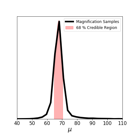
Figure 5: The posterior distribution for the total magnification fitting the multiple-image sncosmo model described in the text. The median value is 67.8 with a 68$\%$ credible region between (64.9, 70.3).

We test the impact of altering the assumption on $R_{V}$. For a fixed $R_{V}=3.1$, corresponding to the MW value, in both the host and lens galaxies, we find host $E(B-V)$ of 0.17 ($\pm$ 0.08) and lens $E(B-V)$ for Images 1, 2, 3 and 4 to be 0.13 ($\pm$ 0.08), 0.20 ($\pm$ 0.09), 0.40 ($\pm$ 0.09), 0.70 ($\pm$ 0.09). We also let the $R_{V}$ in the lens galaxy as a free parameter. The data indicate low lens $R_{V}<1.8$ at 95 $\%$ C.L. Moreover, we fit for the $R_{V}$ for each individual line-of-sight to the four Images. We find that the limits on the $R_{V}$ at 95$\%$ C.L. are $<2.8$, $<3.2$, $<3.6$ and $<1.5$ for Images 1, 2, 3 and 4 respectively. We present details for the impact of dust properties on the inferred magnification in section D.

We also compute the total magnification for iPTF16geu and the magnification of each image. For our fiducial case with both host and lens galaxy $R_{V}=2$, we obtain a median magnification of 67.8 with a 68$\%$ credible region of (64.9, 70.3), plotted in Figure 5. The distributions for the image magnifications are plotted in Figure 6. We test the impact of our assumption on the reddening law. We find that assuming a reddening law from Fitzpatrick (1999, hereafter F99) doesn’t change the total extinction for each image and hence, the inferred total magnification and magnification for each image is consistent with the value derived using the CCM89 dust law. We note, however, that the F99 dust law prefers a lower value of host $E(B-V)$ (and subsequently higher lens $E(B-V)$) than the fiducial case in Table 3. Since a higher host $E(B-V)$ is more consistent with spectroscopic observations (Johansson et al. in prep), we adopt the CCM89 dust law as our fiducial case. Furthermore, we find that the total magnification doesn’t change when leaving both host and lens $R_{V}$ as free parameters and we get a similar constraint of host $R_{V}<1.7$ at the 95$\%$ C.L.

Compared to the model predictions, which find Image 4 to be the brightest and the other three of similar brightness (Mörtsell et al. in prep), we find that the data suggest Image 1 is the brightest followed by Image 2 which is 0.44 times as bright and Images 3 and 4 which have similar brightness 0.2 and 0.26 times that of Image 1, after accounting for extinction corrections in each line of sight. The individual images are magnified by -3.88, -2.99, -2.19, -2.40 magnitudes respectively. We find that the magnification for iPTF16geu is robust to the assumption on the $R_{V}$ for the host and lens galaxies (see Table 3 for individual magnifications for different $R_{V}$ assumptions). The individual image magnifications, using only the space based data are $-3.79^{+0.08}_{-0.07}$, $-2.90^{+0.10}_{-0.09}$, $-2.04^{+0.15}_{-0.15}$ and $-2.33^{+0.12}_{-0.16}$, consistent with the combined constraints.

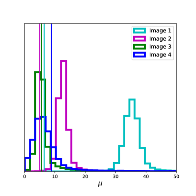
Figure 6: (Left) The observed colour excess for the resolved images in each filter relative to $F814W$ plus the model absorption in the $F814W$ filter compared to the best fit model absorption in each filter assuming the CCM89 dust law. The absorption from the host galaxy dust is plotted in black. For Image 1 we can see that the host galaxy is the dominant source of extinction, and for images 2,3,4 there is a progressively larger contribution from the dust in the lens galaxy. (Right) magnification distribution for the individual images for the fiducial case of host and lens $R_{V}$ fixed to 2 compared to the predictions from the model assuming the lens to be a single isothermal ellipsoid (dashed-dotted lines; see Mörtsell et al in prep for details. The model prediction for $\mu$ of Image 2 has been shifted down by 0.5 so that it can be distinguished from the value for Image 3).

5.2 Time-delays

We fit the time of maximum for the four images to the combination of the resolved $HST$ data and the unresolved ground based data (Equation 1) and calculate the time-delay for images 2, 3 and 4 relative to Image 1, $t_{\rm max,2}$, $t_{\rm max,3}$, $t_{\rm max,4}$. The summary of the parameter values is presented in Table 3. The time-delays for the three images 2, 3 and 4 relative to Image 1 are -0.23, -1.43 and 1.35 days respectively. However, due to the large uncertainties in constraining the time-delays, they are consistent with a zero day time delay at the 95$\%$ C.L. The observed time-delays agree very well with the model predictions suggesting time-delays approximately one day (More et al., 2017, Mörtsell et al. in prep.). We also derive time-delays from the light curves without assuming an SN model. SNe Ia have a distinct light curve morphology in the NIR, showing a second maximum $\sim$ few weeks after the first, we use the timing of this feature to derive constraints on $\Delta_{t}$. Since Images 1 and 2 are the brightest, the NIR light curves only have high enough signal to noise for these two images to derive a time-delay. We use two different methods to fit the data. Firstly, we derive $\Delta_{\rm t}$ using a Gaussian Process (GP) smoothing to the light curve. We use the Matern32 kernel implemented within the GPy package (GPy, 2012), and secondly a cubic spline interpolation. We obtain the timing of the second maximum for each image (and hence, the delay between the two) from the time at which the derivative is zero. The model independent constraints are also consistent with the $\sim$ 1 day time delay derived from fitting the sncosmo model to the data. Using only the $HST$ photometry, we get time-delays for images 2,3,4 of -0.57 ($\pm$ 1.13), -1.47 ($\pm$ 1.07), 0.79 ($\pm$ 1.23) days relative to image 1, consistent with the values from the combination of ground and space-based photometry.

6 Anomalies between observed and predicted flux ratios

The fact that iPTF16geu exploded very close to the inner caustic of the lens makes the predicted radial position, magnification and arrival time very similar for all the images in a smooth lens model. In Goobar et al. (2017), the magnification of the SN images could not be well constrained, but the adopted lens halo predicted brightness differences between the SN images in disagreement with observations. Taking advantage of the improved observational constraints since then, uncertainties in the mass, ellipticity and orientation of the lens galaxy are decreased by a factor $\sim 7$ (Mörtsell et al. in prep).

In table 3, we report the values of the magnifications for each individual image. We find that image 1 is the brightest and 4 is the faintest. Lens models of the system (e.g. More et al., 2017, Mörtsell et al. in prep.) suggest that the SN images would have very similar brightnesses since the SN images are symmetric around the lens. We test whether this could be a result of differential extinction, i.e. a difference in the $R_{V}$ for the dust in the region around Images 1 and 4. Assuming a different $R_{V}$ for images 1 and 4, in this case setting it to extreme values of $R_{V}=1$ and $R_{V}=5$ for images 1 and 4 respectively, we find that Image 4 is still fainter than image 1 by a factor $\sim$ 6 and the best fit value compensates for the high input $R_{V}$ with a lower inferred $E(B-V)$. Moreover, we also fitted for two different $R_{V}$’s in the lens, one for Images 1, 2 and 3 and a separate $R_{V}$ for Image 4. For this case, we get similar values for both $R_{V}$’s and hence, Image 4 is still $\sim$ 9 times fainter than image 1. We note also that deriving constraints assuming an F99 dust law also doesn’t change the observed discrepancy between the brightness of images 1 and 4. Hence, differential extinction is an unlikely explanation for the discrepancy between the observed and modelled image brightness ratios.

In an accompanying paper (Mörtsell et al. in prep), we present lens modelling for iPTF16geu and find that the preferred slope of the projected surface mass density is flatter than a single isothermal ellipsoid profile (Kormann et al., 1994), consistent with the observed time-delays. The observed fluxes cannot be explained by a smooth density profile, regardless of the slope and require a magnification of image 1 by microlensing and a demagnification of images 2, 3 and 4. The differences between the observed fluxes and the smooth density profile are within the stellar microlensing predictions. Discrepancies between the lens macromodel predictions and the observed flux ratios have previously been observed in multiply-imaged quasars, and attributed to microlensing (e.g. in MG 0414+0534; Vernardos, 2018). However, out of the $\sim$ 200 known lensed quasar, only a few have a comparable angular separation to iPTF16geu (see for e.g. Lemon et al., 2018; Lemon et al., 2019). Hence, since iPTF16geu probes high density regions near the core of the galaxy, it is not unusual that the macromodel predictions are discrepant with the observations. While recent studies in the literature find that microlensing can add to the uncertainty in the measured time-delay (Goldstein et al., 2018b; Bonvin et al., 2019), these uncertainties are subdominant compared to the measurement error of $\sim$ 1 day error that we obtain from fitting the data.

7 Implications for observations of future strongly lensed SN

For iPTF16geu, observations that resolved the multiple images only began $\sim$ 2 weeks after maximum light, hence, the light-curve peak in the $HST$ filters is not well determined. Here, we analyse what the constraints on the time-delay and extinction parameters would be if we were to obtain observations close to the peak. We use the best fit model for iPTF16geu to extrapolate the observations near maximum light. We generate ten observations uniformly in the phase region between 10 and 30 days from the first iPTF observations in the P48 R-band. We assume an error on each point to be drawn from a uniform distribution given by the errors on the observed post-maximum epochs. Since the SN is brighter at maximum light we would expect higher signal to noise for similar exposure times and a simpler PSF modeling leading to smaller errors on the fluxes. Under these assumptions we fit the above mentioned sncosmo model to the simulated data. We find that the maximum light data significantly improve the constraints on the time delays, with an error of 0.2 days ($\sim$ 5 hours) which is approximately four times lower than the error from the post-maximum observations. For the expected range of time-delays for ongoing and future surveys between 10 and 50 days (see Goldstein et al., 2018a, for details), this uncertainty corresponds to an error of 2$\%$ or lower in the time-delays, propagated into the $H_{0}$ uncertainty. Since typical model uncertainties in the lens modeling for quasars is $\sim 4\%$ (e.g. Chen et al., 2019; Wong et al., 2019), and knowing the SNe Ia magnification breaks the mass-sheet degeneracy, we can expect a typical $H_{0}$ uncertainty of 3-5$\%$ with the time-delay error having a subdominant contribution. Moreover, studies in the literature (e.g. Goldstein et al., 2018b) find that the impact of microlensing on time-delays is achromatic if the observations are obtained within approximately the first three weeks from explosion. The study finds that the time delay error from microlensing for glSNe in future surveys peaks at $1\%$ for colour curve observations, hence, will be a subdominant contribution in the error budget. Therefore, near maximum observations are crucial for measuring $H_{0}$ precisely from time-delays, especially for highly symmetric systems which have short time-delays, like iPTF16geu.

8 Conclusions

In this paper we present ground-based and $HST$ follow-up of the first resolved, multiply-imaged gravitationally lensed SNe Ia, iPTF16geu. Fitting a multiple image SN Ia model to the data we were able to derive the total magnification, properties of extinction for each image and time-delays between the images. Accounting for the extinction in the individual images, we find that iPTF16geu is amplified by $67.8^{+2.6}_{-2.9}$ times relative to a normal SN Ia at the redshift of the source. Since this value accounts for the extinction in each image separately, it is higher than the first estimate provided in G17. Assuming an $R_{V}=2$ extinction law in the host and lens galaxies, we find an $E(B-V)=0.06$ in Image 1 and 0.17 in Image 2, 0.41 mag in Image 3 and 0.94 mag in Image 4. From the multiple-image model fit, we find that time-delay of images 2, 3 and 4 relative to image 1 to be -0.23 ($\pm$ 0.99), -1.43 ($\pm$ 0.74) and 1.35 ($\pm$ 1.07) days, consistent with the limits presented in G17 and the model predictions in More et al. (2017). We use model independent smoothing techniques to derive the time-delay from the observations of the NIR second maximum and find consistent results with the multiple-image model fit. Furthermore, the total magnification and the time-delay estimates are robust to the assumptions on the host and lens $R_{V}$. We find that the observed difference in the brightness of Images 1 and 2 relative to images 3 and 4 is discrepant with model prediction which suggest a similar brightness for all images. Differential extinction is not sufficient to explain the observed discrepancy. This discrepancy can be possibly resolved with additional substructure lensing; further details are presented in an accompanying paper (Mörtsell et al. in prep). Finally, we presented forecasts for observations of lensed SNe discovered in the future and find that $\sim 10$ $HST$ observations of multiple-image glSNe Ia around maximum light will improve the existing constraints on time-delays by a factor $\sim$ 4.

Appendix A Forward modelling of the iPTF16geu images

In this section we describe the forward model and fitting procedure for iPTF16geu images. A model, $F(r,\phi)$, of the observed 2D shape of the iPTF16geu system in a broadband image, can be expressed as a combination of parametric lens and host models, $L(r,\phi)$ and $H(r,\phi)$, and the point spread function (PSF) of the image as

$$F(r,\phi) = A_{n}\cdot{\rm PSF}\otimes\left[L(r,\phi)+H(r,\phi)\right]+$$

$$+ \sum\limits_{i=1}^{4}\left(f_{i}^{(n)}{\rm PSF}(r_{i},\phi_{i})\right)+B_{n}$$

where the coordinates $(r,\phi)$ are defined with respect to the center (which are treated as nuisance parameters in the fit) of the system in each image $n$, and the angle $0\leq\phi<2\pi$ runs from North towards East. The index, $i=1,2,3,4$ runs over the four SN images, and $n$ runs over all observed epochs for a given band. Furthermore, $f_{i}^{(n)}$ and $(r_{i},\phi_{i})$ are the fluxes and coordinates of the SN images. The amplitude, $A_{n}$, can be used to account for varying photometric calibration, but must be kept fixed for at least one image in each band in order to break the degeneracy between the parameters for $L$ and $H$. We also allow for the background, $B_{n}$ to vary between images.

The lens, $L$, is modelled by a Sérsic profile (Sérsic, 1963)

$$L(r,\phi)=S^{n_{S}}(r,\phi)=f_{S}\cdot\exp\left\{-b_{n}\left[\left(\frac{r_{S}(\theta,\epsilon;\phi)}{r_{e}}\right)^{\frac{1}{2n_{S}}}-1\right]\right\}\,$$ (2)

where $r_{S}(\theta,\epsilon;\phi)$, is generalized to allow for an elliptical model with ellipticity, $\epsilon$, and rotation, $\theta$. Here, $b_{n}$ (solved for numerically) is defined such that $r_{e}$ contains half of the total luminosity , $f_{S}$ is the intensity, and $n_{S}$ is the Sérsic index.

The host galaxy is expressed as a Gaussian profile according to

$$H(x,y)=h\cdot f_{H}(\phi)\cdot\exp\left\{-\frac{(r-r_{H}(\phi))^{2}}{2\sigma_{H}^{2}}\right\}\,,$$ (3)

where the amplitude, $f_{H}(\phi)$ and radius, $r_{H}(\phi)$ are defined as

$$f_{H}(\phi) = \frac{a_{0}}{2}+\sum\limits_{j=1}^{3}a_{j}\cdot\sin(j\phi)+b_{j}\cdot\cos(j\phi)\,,$$ (4)

$$r_{H}(\phi) = \frac{c_{0}}{2}+c_{1}\cdot\sin(\phi)+d_{1}\cdot\cos(\phi)\,.$$ (5)

Table 4: The fitted SN positions to the NIRC2 J-band images. The origin is defined as the origin of the iPTF16geu system as it is obtained from the model fit and the angle, $0\leq\varphi<2\pi$, is defined from North towards East. All quoted uncertainties are statistical errors obtained from the simultaneous fit described in the text.

Image	$r$		$\varphi$
	$(^{\prime\prime})$		(rad)
1	0.251	(0.001)	4.468	(0.002)
2	0.324	(0.001)	2.679	(0.003)
3	0.297	(0.002)	1.013	(0.006)
4	0.276	(0.001)	5.860	(0.005)

Table 5: The fitted lens model parameters as described in eq. (2). The origin $(x_{0}^{(n)},y_{0}^{(n)})$ of the coordinate system are fitted as free parameters for each image $n$. Angles are defined as $0\leq\theta<2\pi$ from North towards East. All quoted uncertainties are statistical fitting errors from each simultaneous fit. Note: Parameters marked with an asterisk (^∗) were fixed to the given value in the fit.

Filter	$f_{S}$		$r_{e}$		$n_{S}$		$\varepsilon$		$\theta$
			$(^{\prime\prime})$						(rad)
$K_{s}$	2.43E$-$01	(1E$-$03)	0.544	(0.001)	0.79	(0.00)	0.165	(0.002)	0.35	(0.01)
$H$	2.08E$-$01	(2E$-$03)	0.585	(0.002)	0.84	(0.01)	0.160	(0.002)	0.30	(0.01)
$F160W$	1.01E$+$01	(4E$-$01)	0.532	(0.010)	1.57	(0.04)	∗0.160		∗0.30
$J$	1.44E$-$01	(1E$-$03)	0.528	(0.002)	0.79	(0.01)	0.127	(0.002)	0.19	(0.01)
$F110W$	1.52E$+$01	(7E$-$01)	0.529	(0.013)	1.66	(0.05)	∗0.127		∗0.19
$F814W$	1.45E$-$01	(9E$-$03)	0.619	(0.026)	1.56	(0.06)	0.252	(0.005)	0.22	(0.01)
$F625W$	1.16E$-$01	(1E$-$03)	0.518	(0.006)	∗1.56		∗0.252		∗0.22
$F475W$	3.69E$-$02	(2E$-$03)	0.474	(0.031)	∗1.56		∗0.252		∗0.22
$F390W$	6.13E$-$03	(1E$-$03)	0.588	(0.147)	∗1.56		∗0.252		∗0.22

Table 6: The fitted parameters of the host model, defined in (3). All quoted uncertainties are statistical fitting errors from each simultaneous fit. Note: Parameters marked with an asterisk (^∗) were fixed to the given value in the fit.

Filter	$a_{0}$		$a_{1}$		$b_{1}$		$a_{2}$		$b_{2}$
$K_{s}$	1.47E$+$00	(1E$-$02)	$-$2.97E$-$01	(3E$-$03)	2.56E$-$01	(3E$-$03)	$-$1.41E$-$01	(2E$-$03)	3.53E$-$02	(2E$-$03)
$H$	5.16E$-$01	(3E$-$03)	$-$1.07E$-$01	(2E$-$03)	8.64E$-$02	(2E$-$03)	$-$4.76E$-$02	(1E$-$03)	1.75E$-$03	(2E$-$03)
$F160W$	1.01E$+$02	(1E$+$00)	$-$1.48E$+$01	(7E$-$01)	2.33E$+$01	(7E$-$01)	$-$2.39E$+$01	(6E$-$01)	4.88E$+$00	(6E$-$01)
$J$	2.78E$-$01	(5E$-$03)	$-$6.93E$-$02	(2E$-$03)	4.75E$-$02	(2E$-$03)	$-$3.43E$-$02	(1E$-$03)	$-$1.52E$-$02	(1E$-$03)
$F110W$	1.40E$+$02	(2E$+$00)	$-$2.28E$+$01	(1E$+$00)	2.62E$+$01	(1E$+$00)	$-$3.85E$+$01	(1E$+$00)	$-$2.03E$+$00	(1E$+$00)
$F814W$	1.41E$+$00	(3E$-$02)	$-$1.11E$-$01	(8E$-$03)	1.15E$-$01	(8E$-$03)	$-$1.51E$-$01	(9E$-$03)	$-$8.07E$-$02	(9E$-$03)
$F625W$	8.06E$-$01	(4E$-$02)	4.52E$-$02	(7E$-$03)	2.73E$-$02	(7E$-$03)	$-$9.13E$-$02	(9E$-$03)	$-$4.77E$-$02	(8E$-$03)
$F475W$	1.07E$-$01	(2E$-$02)	∗0.00E$+$00		∗0.00E$+$00		∗0.00E$+$00		∗0.00E$+$00
Filter	$a_{3}$		$b_{3}$		$c_{0}$		$c_{1}$		$d_{1}$
					$(^{\prime\prime})$		$(^{\prime\prime})$		$(^{\prime\prime})$
$K_{s}$	1.76E$-$01	(2E$-$03)	$-$1.63E$-$01	(3E$-$03)	5.831E$-$01	(3E$-$04)	3.08E$-$02	(3E$-$04)	$-$3.54E$-$02	(3E$-$04)
$H$	5.72E$-$02	(2E$-$03)	$-$4.73E$-$02	(2E$-$03)	5.787E$-$01	(8E$-$04)	3.38E$-$02	(8E$-$04)	$-$3.11E$-$02	(8E$-$04)
$F160W$	$-$1.15E$+$00	(8E$-$01)	$-$1.26E$+$01	(6E$-$01)	∗5.787E$-$01		∗3.38E$-$02		∗$-$3.11E$-$02
$J$	3.46E$-$02	(1E$-$03)	$-$2.00E$-$02	(1E$-$03)	5.911E$-$01	(1E$-$03)	4.49E$-$02	(1E$-$03)	$-$1.69E$-$02	(9E$-$04)
$F110W$	$-$4.29E$-$01	(2E$+$00)	$-$1.54E$+$01	(1E$+$00)	∗5.911E$-$01		∗4.49E$-$02		∗$-$1.69E$-$02
$F814W$	9.74E$-$02	(9E$-$03)	$-$1.71E$-$01	(9E$-$03)	5.784E$-$01	(1E$-$03)	3.51E$-$02	(8E$-$04)	$-$6.58E$-$03	(8E$-$04)
$F625W$	1.74E$-$02	(9E$-$03)	$-$1.13E$-$01	(9E$-$03)	5.788E$-$01	(2E$-$03)	3.28E$-$02	(1E$-$03)	5.30E$-$03	(1E$-$03)
$F475W$	∗0.00E$+$00		∗0.00E$+$00		∗5.788E$-$01		∗3.28E$-$02		∗5.30E$-$03

The parameter $h$, and the parameters $a_{0},a_{j},b_{j}$ cannot be fitted simultaneously. The former is only allowed as a free parameter for WFC3/IR when $a_{0},a_{j},b_{j}$ is fixed to the solution for the LGS-AO data. We use the parametrisation by Moffat (1969) for the PSF. While it is customary to use isolated bright stars in the field to fit the PSF shape, and then fix the model, we are lacking isolated stars (or any objects but the iPTF16geu system) in the narrow field of view NIRC2 images. Hence, the PSF parameters is fitted together with the rest of the parameters of the iPTF16geu model, including the SN fluxes. In other words, the SN images is effectively used to determine the PSF shape. We do not allow the PSF shape parameters to vary between the four SN images. Fitting the PSF shape together with the model will complicate the fitting procedure. While the iPTF16geu model is not expected to vary with time, the observing conditions will, and these are characterised by the differences in the PSFs we are attempting to fit together with the model. We address this by iteratively fitting first the model, and then the PSF shape, to one of our epochs. Once this fit has converged, we use the resulting parameters as initial conditions for the simultaneous fit. For each iteration in the final fitting procedure, the combined model then first convolved with the PSF before it is compared to the data. For the reference images, that are lacking point-sources, we adopt a Gaussian PSF. The width of the Gaussian is fitted together with the other parameters, and the degeneracy between the Gaussian width and and the background model is broken since the same background model is fitted to all epochs simultaneously.

We also allow for a rotation, $\delta_{n}$ of the full system, i.e. $\phi\rightarrow\phi+\delta_{n}$ between images. These parameters must be fixed for at least one image to break the degeneracy with the angle dependent model parameters.

In its most general implementation the number of free parameters of the model can be:

• $2\times n+(n-1)$ for the position and rotation in each image

• $4\times 3\times n$ for the SN fluxes and positions

• $n-1$ for the normalization of the model in each image

• $5$ for the lens model

• $11$ for the host model

which results in a total of $14+16n$ parameters. However, when fitting this model to the data we will generally require that the SN positions are the same between different filters.

Appendix B Empirical point-spread function model for WFC3

Here we describe the point-spread function (PSF) model for the WFC3 data for iPTF16geu. Although the shape and variability of the PSF of WFC3 has been studied in great detail (Anderson, 2016; Anderson & Bedin, 2017), a simple time-independent PSF model will be used here. We fit the profile,

$$PSF(x,y;A,\alpha,\gamma)=A\cdot\frac{\alpha-1}{\pi\gamma^{2}}\left[1+\left(\frac{x^{2}+y^{2}}{\gamma^{2}}\right)\right]^{-\alpha}\,,$$

as described by Moffat (1969), where, $x$ and $y$ are pixel coordinates and $A$, $\alpha$ and $\gamma$ are free parameters. The profile is fitted to bright isolated stars observed between 2010 and 2017 and with the same subarray, UVIS2-C512C-SUB, used for the iPTF16geu. The data are also drizzled to the same resolution, and with the same kernel as for our science observations.

For the WFC3/IR data it is more challenging to fit the full model due to the lower resolution, the broader PSF, and the lower flux ratio between the SN images and the background. The effective radius and the Sérsic index for the lens can be constrained by the light beyond the Einstein ring, but there is a degeneracy between the different components inside the ring. Here, we fixed the $\varepsilon$ and $\theta$ parameters of the lens model for $F110W$ and $F160W$ to the corresponding NIRC2 results for the J and H, respectively, since the effective wavelengths of these filters are similar. Similarly, the radial dependence and the width of the host model were also fixed to the corresponding NIRC2 results.

The WFC3/IR observations of iPTF16geu was obtained with a larger field-of-view than WFC3/UVIS as shown in Fig. 7, and included a bright, but unsaturated, star $\sim 20\arcsec$ North of the object. The star was visible in all WFC3/IR and bands and could be used to determine the PSF shape for these filters using the same approach as for WFC3/UVIS.

The PSF fit is carried out to all data in a given filter. While the amplitude, $A$, is fitted to each exposure, the parameters, $\alpha$ and $\gamma$, are only allowed to vary between different filters. The fitted amplitudes of each star are then compared to the corresponding value obtained from aperture photometry. For the latter we follow the guidelines in the WFC3 data handbook (Deustua, 2016) and always use a fixed aperture radius of $0.4\arcsec$, for which zero points have been derived. The two sets of values are used both to calculate the aperture correction for the PSF photometry and to assess the quality of this simple time-independent PSF model. The latter is quantified by the estimated standard deviation between the PSF and and aperture photometry for all observations in a given filter. These values are then added in quadrature to the photometry error budget.

Since we assume that the PSF is the same for all epochs, we do not convolve the model before comparing with the data in the fitting routine, although doing this will result in similar results. For $F814W$, we fit the same parameters as described in §3.1. For the remaining WFC3/UVIS filters this was not possible, and the lens parameters $n_{S}$, $\varepsilon$ and $\theta$ were then fixed to the results obtained for $F814W$. For $F625W$, we fit all host parameters, while a simplified model with only the first order of angular dependence was used for $F475W$. Furthermore, the radial dependence and the width of the host model was fixed to the results obtained for $F814W$. For $F390W$, the host component was omitted completed. The model complexity for each filter was determined by calculating the impact on the Bayesian Information Criteria (BIC) as more parameters were added. When additional parameters did not impact the BIC, the previous model was selected.

The fitted PSF parameters and the $\sigma$ values are given in Table 7 for the different filters. For the WFC3/IR data the last epoch from 2016, Nov 22 was excluded from the fits since this was found to deviate significantly from the others.

Table 7: Table of the derived PSF parameters and the estimated standard deviations PSF and aperture photometry for all stars in each given. Here, the full width at half maximum was calculated as $\mathrm{FWHM}=2\gamma\left(2^{1/\alpha}-1\right)^{1/2}$. See the text for further details.

Band	$\alpha$	$\gamma$	FWHM	$\sigma$
		(pix)	(pix)	(mag)
F390W	3.245	2.398	2.340	0.072
F475W	3.114	2.531	2.528	0.096
F625W	1.844	1.592	2.151	0.083
F814W	1.798	1.414	1.939	0.024
F110W	2.929	1.343	1.388	0.007
F160W	2.646	1.327	1.452	0.006

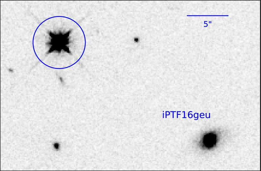
Figure 7: Observation of iPTF16geu in the F110W band obtained on 2016, November 17. The blue circle marks the bright star visible in all IR observations, that was used for determining the aperture correction.

Appendix C Photometry Tables for iPTF16geu

In this section we present the photometry for each of the four resolved images of iPTF16geu as well as the unresolved data from ground-based facilities used for the analyses in this paper.

Table 8: Photometry for the individual resolved images derived from image subtractions using the $HST$ references (see Section 3.3 for details)

MJD	Filter	Flux 1	$\sigma$	Flux 2	$\sigma$	Flux 3	$\sigma$	Flux 4	$\sigma$
(days)		(counts/s)		(counts/s)		(counts/s)		(counts/s)
57685.952	F390W	0.724	0.126	0.352	0.126	0.123	0.126	0.01	0.126
57685.949	F475W	7.639	0.357	2.578	0.317	0.387	0.355	0.182	0.353
57689.921	F475W	6.034	0.183	2.128	0.165	0.397	0.16	0.371	0.167
57685.93	F625W	51.713	0.36	16.248	0.319	3.908	0.311	2.112	0.314
57689.923	F625W	37.214	0.258	12.243	0.231	3.499	0.231	1.674	0.229
57694.217	F625W	31.531	0.141	10.781	0.127	2.702	0.125	1.105	0.124
57698.255	F625W	26.375	0.16	9.073	0.142	2.586	0.14	1.082	0.139
57702.166	F625W	17.133	0.181	8.084	0.168	1.904	0.164	1.094	0.166
57707.131	F625W	17.013	0.153	6.499	0.136	2.518	0.135	1.089	0.135
57709.731	F625W	19.432	0.133	6.586	0.121	1.613	0.119	0.753	0.12
57714.343	F625W	17.807	0.153	6.188	0.14	1.838	0.138	1.142	0.14
57718.186	F625W	16.624	0.151	5.907	0.141	1.737	0.139	0.564	0.141
57685.947	F814W	109.684	0.621	37.694	0.541	11.404	0.532	8.352	0.543
57689.925	F814W	91.459	0.363	32.381	0.306	8.419	0.301	6.558	0.305
57694.219	F814W	84.043	0.239	28.041	0.2	8.525	0.197	6.485	0.199
57698.257	F814W	68.913	0.294	23.438	0.259	6.282	0.256	5.282	0.257
57702.168	F814W	58.245	0.239	17.679	0.223	5.878	0.221	5.173	0.223
57707.133	F814W	46.287	0.299	16.195	0.284	6.057	0.283	4.481	0.284
57709.763	F814W	44.643	0.276	15.938	0.263	4.374	0.261	3.945	0.262
57714.345	F814W	40.195	0.26	13.987	0.235	3.712	0.232	3.043	0.233
57718.189	F814W	36.566	0.253	12.51	0.234	4.537	0.233	3.763	0.235
57681.641	F110W	614.912	17.284	230.826	17.368	84.698	17.163	118.027	17.329
57685.99	F110W	500.802	20.789	282.373	21.0	116.957	20.809	99.238	21.027
57689.965	F110W	641.963	19.965	276.658	19.975	96.479	19.72	87.506	19.761
57694.263	F110W	667.005	12.518	232.676	12.572	93.027	12.386	91.516	12.498
57698.266	F110W	536.644	13.021	191.472	13.091	73.037	12.926	88.226	13.063
57702.175	F110W	381.608	15.014	179.868	15.073	72.463	14.965	80.242	15.051
57707.142	F110W	327.289	24.493	132.207	24.504	53.472	24.458	58.055	24.485
57709.785	F110W	251.143	16.229	142.796	16.249	56.224	16.174	44.146	16.208
57714.354	F110W	253.175	46.9	123.602	46.909	45.288	46.89	31.003	46.901
57718.196	F110W	231.738	12.747	103.494	12.763	44.747	12.702	30.562	12.731
57681.644	F160W	148.62	5.715	64.607	5.728	23.347	5.713	30.422	5.734
57685.992	F160W	149.738	5.307	71.464	5.327	37.903	5.27	24.748	5.318
57689.968	F160W	222.888	6.139	89.367	6.158	36.708	6.108	22.744	6.145
57694.265	F160W	265.299	7.666	106.757	7.685	32.91	7.625	50.389	7.676
57698.269	F160W	239.893	5.68	94.505	5.689	34.862	5.588	52.747	5.654
57702.177	F160W	201.365	6.465	84.814	6.48	30.358	6.462	37.136	6.485
57707.145	F160W	166.162	6.944	74.411	6.952	27.0	6.917	25.435	6.938
57709.787	F160W	139.532	4.371	65.376	4.395	27.973	4.363	23.446	4.402
57714.357	F160W	136.585	23.648	54.621	23.651	24.437	23.651	16.295	23.655
57718.198	F160W	121.397	4.181	48.36	4.193	20.446	4.166	14.082	4.189

Table 9: Ground based photometry from Palomar P48 and P60 and RATIR used in the analyses.

MJD	Filter	Flux	$\sigma$
(days)		(counts/s)
57636.335	P48R	52.481	9.6673
57637.181	P48R	80.91	12.668
57637.329	P48R	83.946	11.598
57638.177	P48R	98.175	10.851
57638.328	P48R	86.298	11.128
57639.227	P48R	114.82	13.747
57639.337	P48R	109.65	10.099
57640.215	P48R	130.62	13.233
57640.324	P48R	130.62	13.233
57641.201	P48R	165.96	18.342
57641.318	P48R	152.76	12.662
57642.196	P48R	205.12	18.892
57642.31	P48R	177.01	17.934
57646.329	P60r	220.8	16.269
57646.331	P60i	277.97	10.241
57646.333	P60g	106.66	12.771
57648.359	P60r	270.4	37.357
57648.361	P60i	325.09	17.965
57648.364	P60g	111.69	16.459
57654.14	P48R	288.4	18.594
57655.115	P48R	283.14	23.47
57655.24	P48R	283.14	18.255
57656.124	P48R	310.46	22.875
57656.25	P48R	277.97	20.482
57657.148	P48R	272.9	17.594
57657.246	P48R	270.4	24.904
57658.132	P48R	280.54	20.671
57658.175	P48R	272.9	17.594
57659.245	P48R	285.76	23.687
57660.149	P48R	251.19	20.822
57661.109	P48R	246.6	20.442
57661.154	P48R	231.21	19.165
57662.104	P48R	265.46	26.895
57662.228	P48R	237.68	17.513
57663.119	P48R	226.99	16.725
57663.222	P48R	224.91	18.643
57664.17	P48R	229.09	18.99
57664.249	P60r	222.84	18.472
57664.251	P60i	346.74	28.742
57664.261	P60r	235.5	13.014
57664.263	P60i	316.23	55.339
57664.264	P60g	48.306	8.0084
57665.294	P60r	205.12	18.892
57665.296	P60i	319.15	91.125
57665.298	P60g	52.966	7.8054
57667.106	P60r	192.31	37.196
57668.099	P48R	203.24	18.719
57668.216	P48R	190.55	17.55
57669.113	P48R	180.3	23.249

MJD	Filter	Flux	$\sigma$
(days)		(counts/s)
57669.146	P60r	144.54	26.626
57670.098	P48R	194.09	25.027
57670.124	J-SPM	482.61	33.45
57670.124	Y-SPM	277.20	33.98
57670.124	i-SPM	252.34	5.51
57670.124	r-SPM	135.89	5.63
57670.124	z-SPM	252.81	11.37
57670.171	P60r	162.93	6.0025
57670.173	P60i	251.19	11.568
57670.174	P60g	25.351	4.2029
57670.225	P60r	145.88	12.093
57670.226	P60i	244.34	51.761
57671.157	Y-SPM	261.57	30.79
57671.157	J-SPM	489.32	35.17
57671.157	i-SPM	249.11	5.44
57671.157	r-SPM	130.25	5.63
57671.157	z-SPM	228.034	11.46
57671.225	P60i	226.99	367.95
57671.235	P60r	125.89	12.755
57671.237	P60i	242.1	187.31
57673.188	P60r	120.23	135.09
57673.189	P60i	222.84	28.735
57673.211	P60r	118.03	13.045
57673.213	P60i	255.86	141.39
57674.123	P60r	131.83	18.212
57674.125	P60i	203.24	11.231
57674.208	P60r	96.383	12.428
57674.21	P60i	237.68	78.809
57675.155	r-SPM	85.90	4.91
57675.155	J-SPM	512.39	35.07
57675.155	Y-SPM	274.15	33.16
57675.155	z-SPM	212.81	11.81
57675.155	i-SPM	210.66	4.98
57680.204	P60r	61.944	89.573
57681.102	P48R	88.716	14.708
57682.096	P48R	81.658	11.282
57682.139	P48R	94.624	12.201
57682.23	P60r	64.863	12.546
57682.231	P60i	145.88	29.56
57683.093	P48R	85.507	11.026
57683.113	r-SPM	50.07	4.41
57683.113	z-SPM	204.36	12.05
57683.113	i-SPM	155.02	4.77
57683.113	Y-SPM	330.82	41.09
57683.113	J-SPM	562.34	34.62
57683.138	P48R	90.365	9.15
57684.151	J-SPM	530.15	34.01
57684.151	Y-SPM	299.22	35.22
57684.151	z-SPM	207.01	11.49
57684.151	i-SPM	153.88	4.74
57684.151	r-SPM	37.84	4.21
57685.116	i-SPM	153.88	4.74
57685.116	J-SPM	575.97	34.96

MJD	Filter	Flux	$\sigma$
(days)		(counts/s)
57685.116	r-SPM	39.12	4.54
57685.116	Y-SPM	313.04	31.72
57685.116	z-SPM	182.97	11.74
57687.117	Y-SPM	320.62	37.22
57687.117	J-SPM	521.91	34.31
57687.117	i-SPM	131.58	4.99
57687.117	z-SPM	196.06	11.56
57687.117	r-SPM	35.35	4.22
57687.13	P60r	39.811	31.534
57687.132	P60i	129.42	10.728
57688.112	r-SPM	35.74	4.32
57688.112	Y-SPM	312.75	44.34
57688.112	z-SPM	185.35	12.53
57688.112	i-SPM	133.17	4.81
57688.113	P60r	40.551	34.361
57688.114	J-SPM	548.02	35.16
57688.115	P60i	120.23	25.469
57690.114	J-SPM	520.47	34.29
57690.114	z-SPM	155.88	11.60
57690.114	r-SPM	26.91	4.03
57690.114	i-SPM	132.80	4.80
57690.114	Y-SPM	367.79	48.63
57691.112	z-SPM	168.73	11.70
57691.112	i-SPM	121.89	4.62
57691.112	r-SPM	22.72	3.93
57691.112	J-SPM	546.01	34.56
57691.112	Y-SPM	301.44	34.02
57692.14	J-SPM	487.08	33.76
57692.14	r-SPM	30.28	4.14
57692.14	z-SPM	145.88	11.36
57692.14	i-SPM	123.25	4.67
57692.14	Y-SPM	330.52	42.12
57693.15	J-SPM	537.53	41.39
57693.15	r-SPM	23.86	4.80
57693.15	z-SPM	117.49	12.87
57693.15	i-SPM	125.77	5.44
57695.108	P60i	84.723	138.12
57695.18	P60i	91.201	21.84
57696.08	P60i	103.75	18.156
57696.082	P60i	148.59	15.055
57697.105	P60r	30.2	54.239
57697.107	P60i	66.069	12.779
57697.109	P60i	85.507	6.3004
57700.096	P60i	114.82	106.81
57702.148	P60i	92.045	22.042
57702.15	P60i	83.176	16.088
57705.163	P60i	80.168	16.244
57723.104	r-SPM	9.72	0.77
57723.104	Y-SPM	132.07	25.99
57723.104	i-SPM	48.26	4.49
57723.104	z-SPM	67.48	11.35
57723.104	Y-SPM	113.76	31.42

Appendix D Lensing galaxy dust properties and image magnifications

In this section, we detail the impact of varying the dust properties for the individual image lines of sight in the lensing galaxy. We analyse the impact that the assumptions have on the inferred magnification.

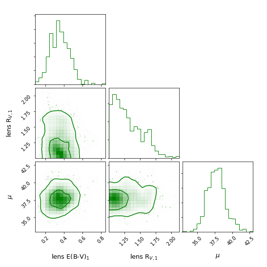
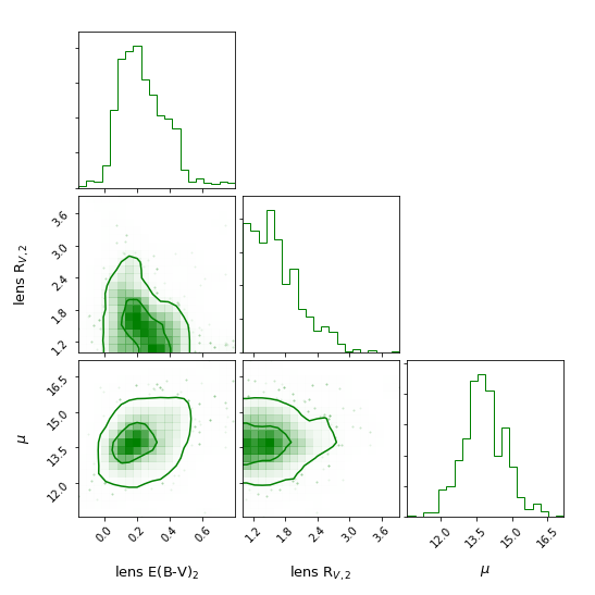
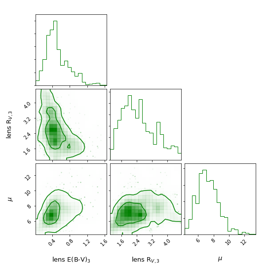
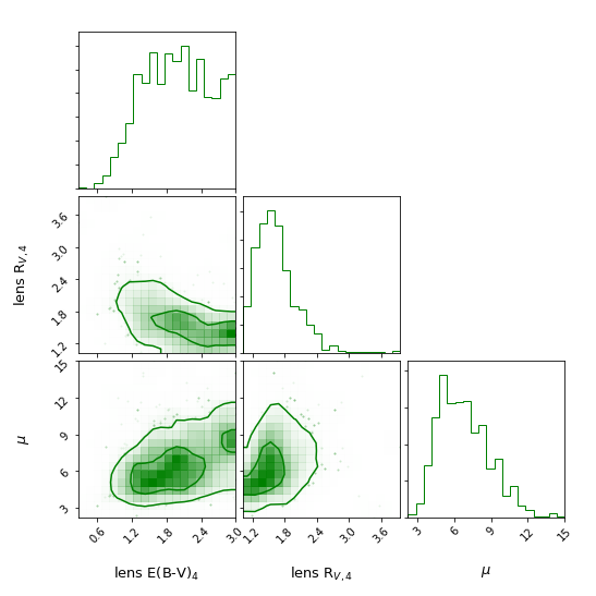
Figure 8: Correlation plots between the inferred colour excess $E(B-V)$, total-to-selective absorption ratio, $R_{V}$, and the magnification, $\mu$ for the images with the $R_{V}$ as a free parameter for each image.

We fit the multiple image model with $R_{V}$ as a free parameter for each of the images, keeping the host galaxy $R_{V}$ fixed to the fiducial case of 2. In Figure 8, we present the correlation between the lens $E(B-V)$, lens $R_{V}$ and the magnification for each image. While the constraints on the $R_{V}$ for Images 1, 2 and 3 are not very stringent, we find that there is a very weak correlation between the $R_{V}$ and $\mu$ for all the images. The inferred total magnification is consistent with the fiducial case of $R_{V}=2$.

In addition, we find that the allowed values of $R_{V}$ for the images do not permit differential extinction between Image 1 and the other Images to explain the discrepancy between the observed and model predicted flux ratios, further suggesting the need for additional lensing from substructures, as discussed in section 6.

References

- Ahn et al. (2012) Ahn C. P., et al., 2012, ApJS, 203, 21
- Anderson (2016) Anderson J., 2016, Technical report, Empirical Models for the WFC3/IR PSF
- Anderson & Bedin (2017) Anderson J., Bedin L. R., 2017, preprint, (arXiv:1706.00386)
- Barbary et al. (2016) Barbary K., et al., 2016, SNCosmo: Python library for supernova cosmology (ascl:1611.017)
- Biscardi et al. (2012) Biscardi I., et al., 2012, A&A, 537, A57
- Bonvin et al. (2019) Bonvin V., Tihhonova O., Millon M., Chan J. H. H., Savary E., Huber S., Courbin F., 2019, A&A, 621, A55
- Butler et al. (2012) Butler N., et al., 2012, in Ground-based and Airborne Instrumentation for Astronomy IV. p. 844610, doi:10.1117/12.926471
- Cano et al. (2018) Cano Z., Selsing J., Hjorth J., de Ugarte Postigo A., Christensen L., Gall C., Kann D. A., 2018, MNRAS, 473, 4257
- Cardelli et al. (1989) Cardelli J. A., Clayton G. C., Mathis J. S., 1989, ApJ, 345, 245
- Chen et al. (2019) Chen G. C. F., et al., 2019, arXiv e-prints, p. arXiv:1907.02533
- DES Collaboration et al. (2018) DES Collaboration et al., 2018, preprint, p. arXiv:1811.02374 (arXiv:1811.02374)
- Deustua (2016) Deustua S. e. a., 2016, Technical report, WFC3 Data Handbook, Version 3.0
- Dhawan et al. (2015) Dhawan S., Leibundgut B., Spyromilio J., Maguire K., 2015, MNRAS, 448, 1345
- Falco et al. (1985) Falco E. E., Gorenstein M. V., Shapiro I. I., 1985, ApJ, 289, L1
- Fitzpatrick (1999) Fitzpatrick E. L., 1999, Publications of the Astronomical Society of the Pacific, 111, 63
- Folatelli et al. (2010) Folatelli G., et al., 2010, AJ, 139, 120
- GPy (2012) GPy since 2012, GPy: A Gaussian process framework in python, http://github.com/SheffieldML/GPy
- Goldstein et al. (2018a) Goldstein D. A., Nugent P. E., Goobar A., 2018a, arXiv e-prints, p. arXiv:1809.10147
- Goldstein et al. (2018b) Goldstein D. A., Nugent P. E., Kasen D. N., Collett T. E., 2018b, ApJ, 855, 22
- Goobar et al. (2017) Goobar A., et al., 2017, Science, 356, 291
- Grillo et al. (2018) Grillo C., et al., 2018, ApJ, 860, 94
- Hamuy et al. (1996) Hamuy M., Phillips M. M., Suntzeff N. B., Schommer R. A., Maza J., Smith R. C., Lira P., Aviles R., 1996, AJ, 112, 2438
- Kelly et al. (2015) Kelly P. L., et al., 2015, Science, 347, 1123
- Kormann et al. (1994) Kormann R., Schneider P., Bartelmann M., 1994, A&A, 284, 285
- Lemon et al. (2018) Lemon C. A., Auger M. W., McMahon R. G., Ostrovski F., 2018, MNRAS, 479, 5060
- Lemon et al. (2019) Lemon C. A., Auger M. W., McMahon R. G., 2019, MNRAS, 483, 4242
- Moffat (1969) Moffat A. F. J., 1969, A&A, 3, 455
- More et al. (2017) More A., Suyu S. H., Oguri M., More S., Lee C.-H., 2017, ApJ, 835, L25
- Oguri (2019) Oguri M., 2019, arXiv e-prints, p. arXiv:1907.06830
- Petrushevska et al. (2017) Petrushevska T., Amanullah R., Bulla M., Kromer M., Ferretti R., Goobar A., Papadogiannakis S., 2017, A&A, 603, A136
- Quimby et al. (2013) Quimby R. M., et al., 2013, ApJ, 768, L20
- Refsdal (1964) Refsdal S., 1964, MNRAS, 128, 307
- Riess et al. (2000) Riess A. G., et al., 2000, ApJ, 536, 62
- Schneider & Sluse (2014) Schneider P., Sluse D., 2014, A&A, 564, A103
- Scolnic et al. (2018) Scolnic D. M., et al., 2018, ApJ, 859, 101
- Sérsic (1963) Sérsic J. L., 1963, Boletin de la Asociacion Argentina de Astronomia La Plata Argentina, 6, 41
- Skrutskie et al. (2006) Skrutskie M. F., et al., 2006, AJ, 131, 1163
- Vernardos (2018) Vernardos G., 2018, MNRAS, 480, 4675
- Watson et al. (2012) Watson A. M., et al., 2012, in Ground-based and Airborne Telescopes IV. p. 84445L, doi:10.1117/12.926927
- Wong et al. (2019) Wong K. C., et al., 2019, arXiv e-prints, p. arXiv:1907.04869