Neutral Higgs decays $H\rightarrow Z\gamma,\gamma\gamma$ in 3-3-1 models

Abstract

The significance of new physics appearing in the loop-induced decays of neutral Higgs bosons into pairs of dibosons $\gamma\gamma$ and $Z\gamma$ will be discussed in the framework of the 3-3-1 models based on a recent work Okada:2016whh , where the Higgs sector becomes effectively the same as that in the two Higgs doublet models (2HDM) after the first symmetry breaking from $SU(3)_{L}$ scale into the electroweak scale. For large $SU(3)_{L}$ scale $v_{3}\simeq 10$ TeV, dominant one-loop contributions to the two decay amplitudes arise from only the single charged Higgs boson predicted by the 2HDM, leading to that experimental constraint on the signal strength $\mu^{331}_{\gamma\gamma}$ of the Standard Model-like Higgs boson decay $h\rightarrow\gamma\gamma$ will result in a strict upper bound on the signal strength $\mu^{331}_{Z\gamma}$ of the decay $h\rightarrow\,Z\gamma$. For a particular model with lower $v_{3}$ around 3 TeV, contributions from heavy charged gauge and Higgs bosons may have the same order, therefore may give strong destructive or constructive correlations. As a by-product, a deviation from the SM prediction $|\mu^{331}_{\gamma\gamma}-1|\leq 0.04$ still allows $|\mu^{331}_{Z\gamma}-1|$ to reach values near 0.1. We also show that there exists an $CP$-even neutral Higgs boson $h^{0}_{3}$ predicted by the 3-3-1 models, but beyond the 2HDM, has an interesting property that the branching ratio Br$(h^{0}_{3}\rightarrow\gamma\gamma)$ is very sensitive to the parameter $\beta$ used to distinguish different 3-3-1 models.

I Introduction

One of the most important channels confirming the existence of the Standard Model-like (SM-like) Higgs boson is the loop-induced decay channel $h\rightarrow\gamma\gamma$. Experimentally, the respective signal strength $\mu_{\gamma\gamma}\equiv(\sigma.\mathrm{Br})_{\mathrm{obs}}/(\sigma.\mathrm{Br})_{\mathrm{SM}}$, which is the observed product of the Higgs boson production cross section ($\sigma$) and its branching ratio (Br) in units of the corresponding values predicted by the standard model (SM) Tanabashi:2018oca , has been updated recently by ATLAS and CMS Aaboud:2018ezd ; Sirunyan:2018ouh ; Aaboud:2018xdt . There is another loop-induced decay $h\rightarrow\,Z\gamma$, which the branching ratio (Br) predicted by the SM is $\mathrm{Br}(h\rightarrow\,Z\gamma)=1.54\times 10^{-3}$ $(\pm 5.7\%)$ corresponding to the Higgs boson mass $m_{h}=125.09$ GeV Heinemeyer:2013tqa ; deFlorian:2016spz . This decay channel has not been observed experimentally. The recent upper constraints of the signal strength are $\mu_{Z\gamma}<6.6$ and $\mu_{Z\gamma}<3.9$ from ATLAS and CMS  Aaboud:2017uhw ; Sirunyan:2018tbk , respectively. In the future project from LHC with its High Luminosity (HL-LHC) and High Energy (HE-LHC), precision measurements for the signal strengths of the two decays $h\rightarrow Z\gamma$ and $h\rightarrow\gamma\gamma$ can reach the respective values of $\mu_{Z\gamma}=1\pm 0.23$ and $\mu_{\gamma\gamma}=1\pm 0.04$ for both ATLAS and CMS Cepeda:2019klc . In addition, the ATLAS expected significance to the $h\rightarrow\,Z\gamma$ channel is hoped to be $4.9~{}\sigma$ with $3000~{}\mathrm{fb}^{-1}$.

In theoretical side, the loop-induced decays of the SM-like Higgs boson mentioned above are important for searching as well as constraining new physics predicted by recent SM extensions, constructed to explain various current experimental data beyond the SM predictions. In the SM, leading contributions to the amplitudes of both decays $h\rightarrow\gamma\gamma,Z\gamma$ are at the one-loop level and relate with $W$ and fermion mediation. On the other hand, SM extensions usually contain new charged particles including scalar, fermions, and gauge bosons spin 1. If any of them couple with the SM-like Higgs boson, they will contribute to the decay amplitude $h\rightarrow\gamma\gamma$ from the one-loop level. Normally, these particles also couple with the SM gauge boson $Z$, hence give one-loop contributions to the decay amplitude $h\rightarrow\,Z\gamma$ too. It seems that the Br of the two decays $h\rightarrow\gamma\gamma,Z\gamma$ have certain relations so that the recent experimental constraint of $\mu_{\gamma\gamma}$ may result in a respective constraint on $\mu_{Z\gamma}$.

The theoretical studies of loop effects caused by new particles on the SM-like Higgs decays including $h\rightarrow\gamma\gamma,Z\gamma$ have been done recently in many SM extensions such as 2HDM Fontes:2014xva ; Kanemura:2018yai ; Bhattacharyya:2013rya ; Bhattacharyya:2014oka , where a thorough investigation in Ref. Fontes:2014xva concerned strong correlations between two signal strengths $\mu_{\gamma\gamma,Z\gamma}$. Hence, the experimental data of $\mu_{\gamma\gamma}$ can be used as an efficient way to predict theoretically constraints on the $\mu_{Z\gamma}$. In left-right models, the decay channel $h\rightarrow\gamma\gamma$ can be used to constrain new heavy charged gauge boson masses Bandyopadhyay:2019jzq . On the other hand, it seems that the result one-loop contribution to the decay amplitude $h\rightarrow Z\gamma$ Martinez:1989kr ; Maiezza:2016bzp has not been discussed for further studying this decay properties using the latest experimental data of the SM-like Higgs boson such as the mass and decay $h\rightarrow\gamma\gamma$. In a recent scotogenic model, new singly and doubly charged Higgs bosons contribute to both loop-induced decay amplitudes $h\rightarrow\gamma\gamma,Z\gamma$ Chen:2019okl . But in this framework, the recent experimental data of the decay $h\rightarrow\gamma\gamma$ predicts a very small a very small deviation from the SM $|\mu_{Z\gamma}-1|<4\%$. In Higgs triplet models Blunier:2016peh , the situation is the same where it was pointed out that Br$(h\rightarrow Z\gamma)$ is usually smaller than Br$(h\rightarrow\gamma\gamma)$. Tiny values of $|\mu_{Z\gamma}-1|$ have been shown recently in other Higgs extensions of the SM Kanemura:2018esc .

In this work, we will focus on another class of the SM extensions, called the 3-3-1 models, which are constructed from the gauge group $\mathbf{SU(3)_{C}}\times SU(3)_{L}\times U(1)_{X}$ Singer:1980sw ; Valle:1983dk ; Pisano:1991ee ; Frampton:1992wt ; Foot:1992rh ; Foot:1994ym . These models have many interesting features which cannot be explained in the SM framework, for example they can give explanations of the existence of three fermion families, the electric charge quantization deSousaPires:1998jc , the sources of CP violations Montero:1998yw ; Montero:2005yb , the strong $CP$-problem Pal:1994ba ; Dias:2002gg ; Dias:2003zt ; Dias:2003iq . In general, one of the most important parameters to distinguish different 3-3-1 models is denoted as $\beta$, which defines electric charges of new particles through the following electric charge operator,

$$Q=T_{3}+\beta T_{8}+X,$$ (1)

where $T_{3}$ and $T_{8}$ are two diagonal generators of the $SU(3)$ group, $X$ is the $U(1)$ charge. Apart from the popular 3-3-1 models with values of $\beta=\pm\frac{1}{\sqrt{3}},\pm\sqrt{3}$, other models with $\beta=0,\pm\frac{2}{\sqrt{3}},\;\frac{1}{3\sqrt{3}}$ have been discussed phenomenologically Hue:2015mna ; Buras:2016dxz ; RamirezBarreto:2019bpx . Different phenomenological aspects in models with arbitrary $\beta$ were also discussed CarcamoHernandez:2005ka ; Cao:2016uur ; Yue:2013qba ; Buras:2014yna ; Buras:2013dea ; Martinez:2014lta ; Hue:2017lak ; Long:2018fud . As we will see, the model contains nine electroweak gauge bosons, four of them are identified as the SM-like particles. The remaining include one heavy neutral gauge boson $Z^{\prime}$ and the two pairs of heavy gauge bosons with electric charges depending on Eq. (1), see a detailed pedagogical calculation in Ref. Buras:2012dp . As usual, all particles get masses from three Higgs $SU(3)_{L}$ triplets, including a neutral $CP$-even Higgs component with a large expectation vacuum value (vev) $v_{3}$ that generates masses for heavy $SU(3)_{L}$ particles. The three Higgs triplets also contain new charged Higgs bosons that may contribute to the amplitudes of the loop-induced decays of neutral Higgs bosons, including the SM-like one. Correlations among these Higgs and gauge contributions will predict the allowed regions of the parameter space satisfying the current experimental data of $h\rightarrow\gamma\gamma$. It is interesting to estimate how large of the allowed values of $\mu_{Z\gamma}$ can be.

The decay $h\rightarrow\gamma\gamma$ was mentioned in some particular 3-3-1 models for constraining the parameter space Caetano:2013nya ; CarcamoHernandez:2019vih . Both $h\rightarrow\gamma\gamma,Z\gamma$ were also mentioned previously in the 3-3-1 models Cao:2016uur ; Yue:2013qba , but some nontrivial contributions to the amplitude of the decay $h\rightarrow\,Z\gamma$ were not included. In this work, we will study effects of heavy particles predicted by the 3-3-1 models on the two signal strengths of the two decays of the SM-like Higgs bosons $h\rightarrow\gamma\gamma,Z\gamma$, using more general analytic formulas of one-loop contributions to the decay amplitude $h\rightarrow\,Z\gamma$ introduced recently Degrande:2017naf ; Hue:2017cph . For simplicity in calculating the physical states of the neutral $CP$-even Higgs bosons, the Higgs potential of the 3-3-1 models will be considered as an effective 2HDM after the first breaking step $SU(3)_{L}\times U(1)_{X}\rightarrow SU(2)_{L}\times U(1)_{Y}$. This form of the Higgs potential was mentioned in detail in Ref. Okada:2016whh for studying a 3-3-1 model with $\beta=-1/\sqrt{3}$. This property of the 3-3-1 models was mentioned previously Martinez:2014lta . The Higgs potential in this limit can be applied to a general 3-3-1 model keeping $\beta$ as a free parameter ($331\beta$). This can be seen by the fact that the model contains two $SU(3)_{L}$ Higgs triplets having components the same as those appear in the 2HDM. The physical states of neutral Higgs bosons then can be determined exactly at the tree level. Recent theoretical constraints on the Higgs sector of 2HDM Haisch:2018djm can be used to constrain the allowed regions of the parameter space relating with those included in the $331\beta$.

On the other hand, the 331$\beta$ contains another heavy neutral Higgs boson $h^{0}_{3}$ that does not couple with SM particles, except the SM-like Higgs boson. Hence, if it is the lightest among those beyond the SM particles, its main decay channels are the tree level decay into a pair of SM-like Higgs boson and loop-induced decays to pairs of gluons and gauge bosons $\gamma\gamma,Z\gamma$. An investigation to determine which decay channels can be used to distinguish different 3-3-1 models will also be presented.

Our work is arranged as follows. Section II summarizes contents of the 3-3-1 models investigated in this work. All couplings and analytic formulas needed for calculating the Brs and signal strengths of the $h,h^{0}_{3}\rightarrow\gamma\gamma,Z\gamma$ are presented in Section III. Numerical results are shown in Section IV. Important remarks and inclusions are pointed out in Section V. Finally, there are three appendices listing more detailed calculations on couplings, particular analytic formulas for one-loop contributions to the decay amplitudes $h,h^{0}_{3}\rightarrow\gamma\gamma,\,Z\gamma$, and interesting numerical illustrations.

II 3-3-1 model with arbitrary $\beta$

II.1 The model review

In this section, we summarize the particle content of the model $331\beta$. Left- and right-handed leptons are assigned to $SU(3)_{L}$ antitriplets and singlets, respectively:

$$L^{\prime}_{aL}=\left(\begin{array}[]{c}e^{\prime}_{a}\\ -\nu^{\prime}_{a}\\ E^{\prime}_{a}\\ \end{array}\right)_{L}\sim\left(1~{},3^{*}~{},-\frac{1}{2}+\frac{\beta}{2\sqrt{3}}\right),\hskip 14.22636pta=1,2,3,$$ (5)

$$e^{\prime}_{aR}\sim\left(1~{},1~{},-1\right),\hskip 14.22636pt\nu^{\prime}_{aR}\sim\left(1~{},1~{},0\right),\hskip 14.22636ptE^{\prime}_{aR}\sim\left(1~{},1~{},-\frac{1}{2}+\frac{\sqrt{3}\beta}{2}\right),$$ (6)

where in the parentheses present the representations and the hypercharge $X$ of the gauge groups $SU(3)_{C}$, $SU(3)_{L}$ and $U(1)_{X}$, respectively. The model includes three right handed (RH) neutrinos $\nu^{\prime}_{aR}$ and heavy exotic leptons $E^{\prime a}_{L,R}$.

The quark sector is arranged to guarantee anomaly cancellation, namely

$$Q^{\prime}_{iL} =\left(\begin{array}[]{c}u^{\prime}_{i}\\ d^{\prime}_{i}\\ J^{\prime}_{i}\\ \end{array}\right)_{L}\sim\left(3,~{}3~{},\frac{1}{6}-\frac{\beta}{2\sqrt{3}}\right),\quad Q^{\prime}_{3L}=\left(\begin{array}[]{c}d^{\prime}_{3}\\ -u^{\prime}_{3}\\ J^{\prime}_{3}\\ \end{array}\right)_{L}\sim\left(3,~{}3^{*}~{},\frac{1}{6}+\frac{\beta}{2\sqrt{3}}\right),$$ (13)

$$u^{\prime}_{aR} \sim\left(3,~{}1~{},\frac{2}{3}\right),\;d^{\prime}_{aR}\sim\left(3,~{}1~{},\frac{-1}{3}\right),$$

$$J^{\prime}_{iR} \sim\left(3,~{}1~{},\frac{1}{6}-\frac{\sqrt{3}\beta}{2}\right),\;J^{\prime}_{3R}\sim\left(3,~{}1~{},\frac{1}{6}+\frac{\sqrt{3}\beta}{2}\right),$$ (14)

where $i=1,2$, $a=1,2,3$, and $J_{aL,R}$ are exotic quarks predicted by the 331$\beta$ model. There is another arrangement that the model contains three left-handed lepton $SU(3)_{L}$ triplets, one quark $SU(3)_{L}$ triplet and two other quark $SU(3)_{L}$ antitriplets. But, it was shown that the two arrangements are equivalent in the sense that they predict the same physics Descotes-Genon:2017ptp ; Hue:2018dqf .

To generate masses for gauge bosons and fermions, three scalar triplets are introduced as follows

$$\chi =\left(\begin{array}[]{c}\chi^{+A}\\ \chi^{+B}\\ \chi^{0}\\ \end{array}\right)\sim\left(1,~{}3~{},\frac{\beta}{\sqrt{3}}\right),\quad\rho=\left(\begin{array}[]{c}\rho^{+}\\ \rho^{0}\\ \rho^{-B}\\ \end{array}\right)\sim\left(1,~{}3~{},\frac{1}{2}-\frac{\beta}{2\sqrt{3}}\right),$$ (21)

$$\eta =\left(\begin{array}[]{c}\eta^{0}\\ \eta^{-}\\ \eta^{-A}\\ \end{array}\right)\sim\left(1,~{}3~{},-\frac{1}{2}-\frac{\beta}{2\sqrt{3}}\right),$$ (25)

where $A,B$ denote electric charges defined in Eq. (1): $A=\frac{1+\beta\sqrt{2}}{2}$ and $B=\frac{-1+\beta\sqrt{2}}{2}$. These Higgs bosons develop vevs defined as $\langle\chi^{0}\rangle=\frac{v_{3}}{\sqrt{2}},\,\langle\rho^{0}\rangle=\frac{v_{2}}{\sqrt{2}},\,\langle\eta^{0}\rangle=\frac{v_{1}}{\sqrt{2}}$, leading to

$$\chi^{0} =\frac{v_{3}+r_{3}+ia_{3}}{\sqrt{2}},\quad\langle\rho^{0}\rangle=\frac{v_{2}+r_{2}+ia_{2}}{\sqrt{2}},\quad\langle\eta^{0}\rangle=\frac{v_{1}+r_{1}+ia_{1}}{\sqrt{2}}.$$ (26)

The symmetry breaking happens in two steps: $SU(3)_{L}\otimes U(1)_{X}\xrightarrow{v_{3}}SU(2)_{L}\otimes U(1)_{Y}\xrightarrow{v_{1},v_{2}}U(1)_{Q}$. It is therefore reasonable to assume that $v_{3}>v_{1},v_{2}$. At the second breaking step, $\rho$ and $\eta$ play roles of the two $SU(2)_{L}$ doublets similar to 2HDM, except differences in coupling with fermions. Masses and physical states of all particles are summarized as follows.

II.2 Fermions

Masses and physical states of the fermions are derived from the following Yukawa Lagrangian

$$\mathcal{L}^{Y}_{\mathrm{lepton}} =-Y^{e}_{ab}\overline{L^{\prime}}_{aL}\eta^{*}e^{\prime}_{bR}-Y^{\nu}_{ab}\overline{L^{\prime}}_{aL}\rho^{*}\nu^{\prime}_{bR}-Y^{E}_{ab}\overline{L^{\prime}}_{aL}\chi^{*}E^{\prime}_{bR}+\mathrm{h.c.},$$ (27)

$$\mathcal{L}^{Y}_{\mathrm{quark}} =-Y^{d}_{ia}\overline{Q^{\prime}}_{iL}\rho d^{\prime}_{aR}-Y^{d}_{3a}\overline{Q^{\prime}}_{3L}\eta^{*}d^{\prime}_{aR}-Y^{u}_{ia}\overline{Q^{\prime}}_{iL}\eta u_{aR}-Y^{u}_{3a}\overline{Q^{\prime}}_{3L}\rho^{*}u^{\prime}_{aR}$$

$$-Y^{J}_{ij}\overline{Q^{\prime}}_{iL}\chi J^{\prime}_{jR}-Y^{J}_{33}\overline{Q^{\prime}}_{3L}\chi^{*}J^{\prime}_{3R}+\mathrm{h.c.},$$ (28)

We note that depending on particular values of $\beta$, additional Yukawa terms may appear but a $Z_{2}$ symmetry can be imposed to exclude them, see an example given in Ref. Okada:2016whh .

As mentioned above, the SM-like fermions get masses from their couplings to two Higgs triplets $\eta$ and $\rho$, similarly to the 2HDM. On the other hand, the up (down) quarks couple to both Higgs triplets, leading to a different feature from four popular types of 2HDM, where all up (down) quarks couple to the same Higgs doublet in order to avoid tree level flavor changing neutral currents (FCNCs), see for example in Ref. Craig:2012vn . As a result, many interesting properties relating with the SM-like fermion couplings were pointed out to distinguish 3-3-1 models and 2HDMs Okada:2016whh .

The exotic fermions couple to only the Higgs triplet $\chi$. Accordingly, the neutral Higgs sector in Ref. Okada:2016whh has a property that the $\chi^{0}$ does not contribute to the SM-like Higgs boson, it therefore decouples with all exotic fermions. Hence, they do not contribute to the one-loop decay amplitudes $h\rightarrow\gamma\gamma,Z\gamma$.

The SM-like fermion masses are determined based on discussions in refs. Okada:2016whh ; Buras:2012dp ; Hue:2017lak , where the mixing between quarks are safely ignored in this work. Then all fermion mass matrices are diagonal. Correspondingly, the original fermion states are physical, hence they will be denoted by $e_{aL,R},u_{aL,R}$ and $d_{aL,R}$. The fermion masses are given as follows:

$$m_{e_{a}} =\frac{Y^{e}_{aa}v_{1}}{\sqrt{2}},\;m_{u_{i}}=\frac{Y^{u}_{ii}v_{1}}{\sqrt{2}},\;m_{d_{i}}=\frac{Y^{d}_{ii}v_{2}}{\sqrt{2}},\;m_{u_{3}}=-\frac{Y^{u}_{33}v_{2}}{\sqrt{2}},\;m_{d_{3}}=\frac{Y^{d}_{33}v_{1}}{\sqrt{2}},\;m_{F_{a}}=\frac{Y^{F}_{aa}v_{3}}{\sqrt{2}},$$ (29)

where $Y^{f}_{ab}=0~{}\forall a\neq b$, $f=e,u,d,F$ and $F=J,E$. The relations (29) will be used to determine Feynman rules of Yukawa couplings in Lagrangians (27) and (28).

II.3 Gauge bosons

The model contains nine electroweak (EW) gauge bosons corresponding to the 9 generators of the EW gauge group $SU(3)_{L}\otimes U(1)_{X}$. The covariant derivative is defined as Buras:2012dp ; Hue:2017lak ; Cao:2016uur ,

$$D_{\mu}\equiv\partial_{\mu}-igT^{a}W^{a}_{\mu}-ig_{X}XT^{9}X_{\mu},$$ (30)

where $T^{9}=1/\sqrt{6}$, $g$ and $g_{X}$ are coupling constants of the two groups $SU(3)_{L}$ and $U(1)_{X}$, respectively. The matrix $W^{a}T^{a}$, where $T^{a}=\lambda_{a}/2$ corresponding to a triplet representation, is

$$W^{a}_{\mu}T^{a}=\frac{1}{2}\left(\begin{array}[]{ccc}W^{3}_{\mu}+\frac{1}{\sqrt{3}}W^{8}_{\mu}&\sqrt{2}W^{+}_{\mu}&\sqrt{2}Y^{+A}_{\mu}\\ \sqrt{2}W^{-}_{\mu}&-W^{3}_{\mu}+\frac{1}{\sqrt{3}}W^{8}_{\mu}&\sqrt{2}V^{+B}_{\mu}\\ \sqrt{2}Y^{-A}_{\mu}&\sqrt{2}V^{-B}_{\mu}&-\frac{2}{\sqrt{3}}W^{8}_{\mu}\\ \end{array}\right),$$ (34)

where we have defined the mass eigenstates of the nondiagonal gauge bosons as

$$W^{\pm}_{\mu}=\frac{1}{\sqrt{2}}\left(W^{1}_{\mu}\mp iW^{2}_{\mu}\right),\;Y^{\pm A}_{\mu}=\frac{1}{\sqrt{2}}\left(W^{4}_{\mu}\mp iW^{5}_{\mu}\right),\;V^{\pm B}_{\mu}=\frac{1}{\sqrt{2}}\left(W^{6}_{\mu}\mp iW^{7}_{\mu}\right),$$ (35)

and $A,B$ are electric charges of the corresponding gauge bosons calculated based on Eq. (1),

$$A=\frac{1}{2}+\beta\frac{\sqrt{3}}{2},\quad B=-\frac{1}{2}+\beta\frac{\sqrt{3}}{2}.$$ (36)

We note that $B$ is also the electric charge of the new leptons $E_{a}$.

The symmetry breaking happens in two steps: $SU(3)_{L}\otimes U(1)_{X}\xrightarrow{v_{3}}SU(2)_{L}\otimes U(1)_{Y}\xrightarrow{v_{1},v_{2}}U(1)_{Q}$, corresponding to the following transformation of the neutral gauge bosons form the original basis to the final physical one: $X_{\mu},\,W^{3}_{\mu},\,W^{8}_{\mu}\xrightarrow{\theta_{331}}\,B_{\mu},\,W^{3}_{\mu},\,Z^{\prime}_{\mu}\xrightarrow{\theta_{W}}A_{\mu},\,Z_{\mu},\,Z^{\prime}_{\mu}\xrightarrow{\theta}A_{\mu},\,Z_{1\mu},\,Z_{2\mu}$. After the first step, five gauge bosons will be massive and the remaining four massless gauge bosons can be identified with the before-symmetry-breaking SM gauge bosons. The two physical states $Z_{1,2}$ are mixed from the SM and heavy gauge bosons $Z_{\mu}$ and $Z^{\prime}_{\mu}$.

It is well-known that

$$g_{2}=g,\quad g_{1}=g_{X}\frac{g}{\sqrt{6g^{2}+\beta^{2}g_{X}^{2}}},$$ (37)

where $g_{2}$ and $g_{1}$ are the two couplings of the of the SM gauge groups $SU(2)_{L}$ and $U(1)_{Y}$, respectively. Using the weak mixing angle defined as $t_{W}=\tan\theta_{W}=g_{1}/g_{2}$ and denoting $s_{W}=\sin\theta_{W}$ and $c_{W}=\cos\theta_{W}$, it is derived that

$$\frac{g_{X}^{2}}{g^{2}}=\frac{6s_{W}^{2}}{1-(1+\beta^{2})s_{W}^{2}}=\frac{6s_{W}^{2}}{c^{2}_{W}(1-\beta^{2}t^{2}_{W})},$$ (38)

which gives a constraint $|\beta|\leq\sqrt{3}$ used in the numerical analysis.

The masses of the gauge bosons given in (35) are

$$m^{2}_{Y}\equiv m^{2}_{Y^{\pm A}}=\frac{g^{2}}{4}(v_{3}^{2}+v_{1}^{2}),\;m^{2}_{V}\equiv\ m^{2}_{V^{\pm B}}=\frac{g^{2}}{4}(v_{3}^{2}+v_{2}^{2}),\;m^{2}_{W}\equiv m^{2}_{W^{\pm}}=\frac{g^{2}}{4}(v_{1}^{2}+v^{2}_{2}).$$ (39)

The matching condition with the SM gives $v^{2}\equiv v_{1}^{2}+v_{2}^{2}\simeq 246\,[\mathrm{GeV}^{2}]$. Based on Refs. Buras:2012dp ; Buras:2014yna , the ratios between vevs are used to define three mixing parameters as follows

$$s_{ij}\equiv \frac{v_{i}}{\sqrt{v_{i}^{2}+v_{j}^{2}}},\;c_{ij}\equiv\sqrt{1-s^{2}_{ij}},\quad t_{ij}\equiv\tan\beta_{ij}=\frac{s_{ij}}{c_{ij}},$$ (40)

where $i<j$ and $i,j=1,2,3$.

The model predicts three neutral gauge bosons including the massless photon. Defining Buras:2012dp

$$s_{331}\equiv\sin\theta_{331} =\frac{\sqrt{6}g}{\sqrt{6g^{2}+\beta^{2}g_{X}^{2}}}=\sqrt{1-\beta^{2}t_{W}^{2}},\;c_{331}\equiv\cos\theta_{331}=\beta t_{W},$$ (41)

the relation between the original and physical base of the neutral gauge bosons are

$$\begin{pmatrix}X_{\mu}\\ W^{3}_{\mu}\\ W^{8}_{\mu}\end{pmatrix} =\begin{pmatrix}s_{331}&0&c_{331}\\ 0&1&0\\ c_{331}&0&-s_{331}\end{pmatrix}\begin{pmatrix}c_{W}&-s_{W}&0\\ s_{W}&c_{W}&0\\ 0&0&1\end{pmatrix}\begin{pmatrix}1&0&0\\ 0&c_{\theta}&-s_{\theta}\\ 0&s_{\theta}&c_{\theta}\end{pmatrix}\begin{pmatrix}A_{\mu}\\ Z_{1\mu}\\ Z_{2\mu}\end{pmatrix}=C\begin{pmatrix}A_{\mu}\\ Z_{1\mu}\\ Z_{2\mu}\end{pmatrix},$$

$$C =\begin{pmatrix}s_{331}c_{W},&\left(-s_{331}s_{W}c_{\theta}+c_{331}s_{\theta}\right),&\left(s_{331}s_{W}s_{\theta}+c_{331}c_{\theta}\right)\\ s_{W},&c_{W}c_{\theta},&-s_{\theta}c_{w}\\ c_{331}c_{W},&-\left(c_{331}s_{W}c_{\theta}+s_{331}s_{\theta}\right),&\left(c_{331}s_{W}s_{\theta}-s_{331}c_{\theta}\right)\end{pmatrix},$$ (42)

where in the limit $v^{2}\ll v_{3}^{2}$, the mixing angle $\theta$ is determined as Buras:2014yna

$$s_{\theta}\equiv\sin\theta =\left(3\beta\frac{s_{W}^{2}}{c_{W}^{2}}+\frac{\sqrt{3}(t^{2}_{21}-1)}{t^{2}_{21}+1}\right)\frac{\sqrt{1-\beta^{2}t_{W}^{2}}v^{2}}{4c_{W}v_{3}^{3}},$$ (43)

and $M^{2}_{Z^{\prime}}=g^{2}v^{2}_{3}/(3s^{2}_{331})+\mathcal{O}(v^{2})$.

To continue, the neutral gauge bosons will be identified as $Z_{1}\equiv Z$ and $Z_{2}\equiv Z^{\prime}$, where $Z$ is the one found experimentally.

II.4 Higgs bosons

The scalar potential is

$$V_{h} = \mu_{1}^{2}\eta^{\dagger}\eta+\mu_{2}^{2}\rho^{\dagger}\rho+\mu_{3}^{2}\chi^{\dagger}\chi+\lambda_{1}\left(\eta^{\dagger}\eta\right)^{2}+\lambda_{2}\left(\rho^{\dagger}\rho\right)^{2}+\lambda_{3}\left(\chi^{\dagger}\chi\right)^{2}$$ (44)

$$+ \lambda_{12}(\eta^{\dagger}\eta)(\rho^{\dagger}\rho)+\lambda_{13}(\eta^{\dagger}\eta)(\chi^{\dagger}\chi)+\lambda_{23}(\rho^{\dagger}\rho)(\chi^{\dagger}\chi)$$

$$+ \tilde{\lambda}_{12}(\eta^{\dagger}\rho)(\rho^{\dagger}\eta)+\tilde{\lambda}_{13}(\eta^{\dagger}\chi)(\chi^{\dagger}\eta)+\tilde{\lambda}_{23}(\rho^{\dagger}\chi)(\chi^{\dagger}\rho)-\sqrt{2}f\left(\epsilon_{ijk}\eta^{i}\rho^{j}\chi^{k}+\mathrm{h.c.}\right).$$

The minimum conditions of the Higgs potential can be figured out easily Buras:2012dp ; Hue:2017lak . After that, we can take $\mu_{i}^{2}$ as functions of other independent parameters. These functions are inserted into the Higgs potential (44), which is used to determine the masses and physical states of all Higgs bosons.

The relations between original and mass eigenstates of charged Higgs bosons are Buras:2012dp ; Hue:2017lak :

$$\left(\begin{array}[]{c}\phi^{\pm}_{W}\\ H^{\pm}\\ \end{array}\right) =R(\beta_{12})\left(\begin{array}[]{c}\rho^{\pm}\\ \eta^{\pm}\\ \end{array}\right),\;m_{\phi_{W}}=0,\;m^{2}_{H^{\pm}}=\frac{\tilde{\lambda}_{12}v^{2}}{2}+\frac{fv_{3}}{2s_{12}c_{12}},$$ (49)

$$\left(\begin{array}[]{c}\phi^{\pm A}_{Y}\\ H^{\pm A}\\ \end{array}\right) =R(\beta_{13})\left(\begin{array}[]{c}\chi^{\pm A}\\ \eta^{\pm A}\\ \end{array}\right),\;m_{\phi_{Y}}=0,\;m^{2}_{H^{\pm A}}=\left(\frac{\tilde{\lambda}_{13}}{2}+\frac{f}{t_{12}v_{3}}\right)\left(v_{1}^{2}+v_{3}^{2}\right),$$ (54)

$$\left(\begin{array}[]{c}\phi^{\pm B}_{V}\\ H^{\pm B}\\ \end{array}\right) =R(\beta_{23})\left(\begin{array}[]{c}\chi^{\pm B}\\ \rho^{\pm B}\\ \end{array}\right),\;m_{\phi_{V}}=0,\;m^{2}_{H^{\pm B}}=\left(\frac{\tilde{\lambda}_{23}}{2}+\frac{t_{12}f}{v_{3}}\right)\left(v_{2}^{2}+v_{3}^{2}\right),$$ (59)

where we have define a rotation $R(x)$ as

$$R(x)\equiv\left(\begin{array}[]{cc}c_{x}&-s_{x}\\ s_{x}&c_{x}\\ \end{array}\right).$$ (60)

The massless states $\phi^{\pm}_{W}$, $\phi^{\pm A}_{Y}$, and $\phi^{\pm\,B}_{V}$ are Goldstone bosons absorbed by the physical gauge bosons.

For neutral Higgs bosons, to avoid the tree level contribution of SM-like Higgs bosons to the flavor changing neutral currents (FCNC) in the quark sector, we follow the aligned limit introduced in Ref. Okada:2016whh , namely

$$f=\lambda_{13}t_{12}v_{3}=\frac{\lambda_{23}v_{3}}{t_{12}}.$$ (61)

From this, we will choose $f$ and $\lambda_{23}$ as functions of the remaining, leading to the following form of the squared mass matrix corresponding to the basis $(r_{1},r_{2},r_{3})$:

$$M^{2}_{r}=\begin{pmatrix}2\lambda_{1}s^{2}_{12}v^{2}+\lambda_{13}v_{3}^{2}&t_{12}\left(\lambda_{12}c_{12}^{2}v^{2}-\lambda_{13}v_{3}^{2}\right)&0\\ t_{12}\left(\lambda_{12}c_{12}^{2}v^{2}-\lambda_{13}v_{3}^{2}\right)&2c^{2}_{12}\lambda_{2}v^{2}+t^{2}_{12}\lambda_{13}v_{3}^{2}&0\\ 0&0&s_{12}^{2}\lambda_{13}v^{2}+2\lambda_{3}v_{3}^{2}\end{pmatrix}.$$ (62)

As a result, $r_{3}\equiv h^{0}_{3}$ is a physical $CP$-even neutral Higgs boson with mass $m^{2}_{h^{0}_{3}}=\lambda_{13}s^{2}_{12}v^{2}+2\lambda_{3}v_{3}^{2}$. The submatrix $2\times 2$ in Eq. (62) is denoted as $M^{\prime 2}_{r}$. It is diagonalized as follows Okada:2016whh ,

$$R(\alpha)M^{\prime 2}_{r}R^{T}(\alpha)=\mathrm{diag}(m^{2}_{h^{0}_{1}},m^{2}_{h^{0}_{2}}),$$ (63)

where

$$\alpha \equiv\beta_{12}-\frac{\pi}{2}+\delta,$$ (64)

$$\tan 2\delta =\frac{2M^{2}_{12}}{M^{2}_{22}-M^{2}_{11}}\sim\mathcal{O}\left(\frac{v^{2}}{v_{3}^{2}}\right),$$ (65)

$$m^{2}_{h^{0}_{1}} =M^{2}_{11}\cos^{2}\delta+M^{2}_{22}\sin^{2}\delta-M^{2}_{12}\sin 2\delta,$$ (66)

$$m^{2}_{h^{0}_{2}} =M^{2}_{11}\sin^{2}\delta+M^{2}_{22}\cos^{2}\delta+M^{2}_{12}\sin 2\delta,$$ (67)

$$M^{2}_{11} =2\left(s_{12}^{4}\lambda_{1}+c_{12}^{4}\lambda_{2}+s_{12}^{2}c_{12}^{2}\lambda_{12}\right)v^{2}=\mathcal{O}(v^{2}),$$

$$M^{2}_{12} =\left[-\lambda_{1}s^{2}_{12}+\lambda_{2}c^{2}_{12}+\lambda_{12}(s^{2}_{12}-c^{2}_{12})\right]s_{12}c_{12}v^{2}=\mathcal{O}(v^{2}),$$

$$M^{2}_{22} =2s^{2}_{12}c^{2}_{12}\left[\lambda_{1}+\lambda_{2}-\lambda_{12}\right]v^{2}+\frac{\lambda_{13}v^{2}_{3}}{c^{2}_{12}}.$$

We also have

$$\left(\begin{array}[]{c}r_{1}\\ r_{2}\\ \end{array}\right) =R^{T}(\alpha)\left(\begin{array}[]{c}h^{0}_{1}\\ h^{0}_{2}\\ \end{array}\right).$$ (72)

To determine the SM-like Higgs boson, we first look at the Eq. (65), which give $\delta=\mathcal{O}(\frac{v^{2}}{v_{3}^{2}})\simeq 0$ when $v^{2}\ll v_{3}^{2}$. In this limit, $m^{2}_{h}=M^{2}_{11}+v^{2}\times\mathcal{O}(\frac{v^{2}}{v_{3}^{2}})\sim M^{2}_{11}$ while $m^{2}_{h^{0}_{2}}=M^{2}_{22}+v^{2}\times\mathcal{O}(\frac{v^{2}}{v_{3}^{2}})\simeq M^{2}_{22}$. Hence, $h^{0}_{1}\equiv\,h$ is identified with the SM-like Higgs boson found at LHC. Furthermore, in the following calculation we will see more explicitly that the couplings of this Higgs boson are the same as those given in the SM in the limit $\delta\rightarrow 0$.

Because the two mass matrices $M^{\prime 2}_{r}$ given in Eqs. (62) and the one given in Eq. (63) differ from each other by the unitary transformation $R(\alpha)$, their traces are equal, namely Tr$[M^{\prime 2}_{r}]=\mathrm{Tr}[R(\alpha)M^{\prime 2}_{r}R^{T}(\alpha)]=m^{2}_{h^{0}_{1}}+m^{2}_{h^{0}_{2}}$. Accordingly, $\lambda_{13}$ can be written as

$$\lambda_{13}=\frac{c^{2}_{12}}{v_{3}^{2}}\left[m^{2}_{h^{0}_{1}}+m^{2}_{h^{0}_{2}}-2v^{2}\left(s_{12}^{2}\lambda_{1}+c_{12}^{2}\lambda_{2}\right)\right].$$ (73)

We will choose $\delta$, $m_{h^{0}_{1}}\equiv m_{h}$ and $m_{h^{0}_{2}}$ as input parameters. The $\lambda_{13}$, $\lambda_{12}$ and $\lambda_{2}$ are dependent parameters, namely

$$\lambda_{2} =t^{4}_{12}\lambda_{1}+\frac{-\left[c^{2}_{\delta}(t^{2}_{12}-1)+t_{12}s_{2\delta}\right]m^{2}_{h}+\left[s^{2}_{\delta}(1-t^{2}_{12})+s_{2\delta}t_{12}\right]m^{2}_{h^{0}_{2}}}{2c^{2}_{12}v^{2}},$$

$$\lambda_{12} =-2t^{2}_{12}\lambda_{1}+\frac{\left(s_{2\delta}+2t_{12}c^{2}_{\delta}\right)m^{2}_{h}+\left(-s_{2\delta}+2t_{12}s^{2}_{\delta}\right)m^{2}_{h^{0}_{2}}}{2s_{12}c_{12}v^{2}},$$ (74)

and $\lambda_{13}$ was given in Eq. (73).

The Higgs self-couplings should satisfy all constraints discussed recently to guarantee the vacuum stability of the Higgs potential Sanchez-Vega:2018qje , the perturbative limits, and the positive squared masses of all Higgs bosons. We note that in the case of absence the relations in Eq. (61), the mixing between SM-like Higgs bosons with other heavy neutral Higgs still suppressed due to large $v_{3}>5$ TeV enoungh to cancel the FCNCs in 3-3-1 models Huitu:2019kbm .

III Couplings and analytic formulas involved with loop-induced Higgs decays

III.1 Couplings

From the above discussion on the Higgs potential, we can derive all Higgs self-couplings of the SM-like Higgs boson relating to the decays $h\rightarrow Z\gamma$ and $h\rightarrow\gamma\gamma$, using the interacting Lagrangian $\mathcal{L}_{hHH}=-V_{h}$. The Feynman rules are given in Table 1, where each factor $-i\lambda_{hss}$ corresponds to a vertex $hss$, where $s=H^{\pm},H^{\pm A},H^{\pm B}$.

Vertex	Coupling: $-i\lambda_{hss}$
$-i\lambda_{hH^{+}H^{-}}$	$iv\left[2s_{12}c_{12}\left(-\lambda_{1}c_{12}\,c_{\alpha}+\lambda_{2}s_{12}\,s_{\alpha}\right)+\left(s_{\alpha}c^{3}_{12}-c_{\alpha}s^{3}_{12}\right)\lambda_{12}-c_{\delta}\tilde{\lambda}_{12}\right]$
$-i\lambda_{hH^{A}H^{-A}}$	$ic^{2}_{13}\left\{v\left[s_{\alpha}c_{12}\left(\lambda_{12}+t^{2}_{13}\lambda_{23}\right)-c_{\alpha}s_{12}\left(2\lambda_{1}+t^{2}_{13}(\lambda_{13}+\tilde{\lambda}_{13})\right)\right]+v_{3}t_{13}\left(\frac{2fs_{\alpha}}{v_{3}}-c_{\alpha}\tilde{\lambda}_{13}\right)\right\}$
$-i\lambda_{hH^{B}H^{-B}}$	$ic^{2}_{23}\left\{v\left[s_{\alpha}c_{12}\left(2\lambda_{2}+t^{2}_{23}(\lambda_{23}+\tilde{\lambda}_{23})\right)-c_{\alpha}s_{12}\left(\lambda_{12}+t^{2}_{23}\lambda_{13}\right)\right]+v_{3}t_{23}\left(s_{\alpha}\tilde{\lambda}_{23}-\frac{2fc_{\alpha}}{v_{3}}\right)\right\}$

Table 1: Feynman rules for the SM-like Higgs boson couplings with charged Higgs bosons

Based on the Yukawa Lagrangians (27) and (28), the couplings of the SM-like Higgs boson with SM fermions can be determined, see also in table 1, where we have used the relation (64). The notation of the Feynman rule is $-i\left(Y_{h\bar{f}fL}P_{L}+Y_{h\bar{f}fR}P_{R}\right)$ for each vertex $h\bar{f}f$. For simplicity, the Yukawa couplings of the SM-like fermions in this case were identified with those in the SM, as discussed before. Then, we have $Y_{\bar{f}fL}=Y_{\bar{f}fR}$, which are given in table 2.

	$-iY_{h\overline{e_{a}}e_{a}L,R}$	$-iY_{h\overline{u_{i}}u_{i}L,R}$	$-iY_{h\overline{u_{3}}u_{3}L,R}$	$-iY_{h\overline{d_{i}}d_{i}L,R}$	$-iY_{h\overline{d_{3}}d_{3}L,R}$
	$-i\frac{m_{e_{a}}}{v}\left(c_{\delta}-\frac{s_{\delta}}{t_{12}}\right)$	$-i\frac{m_{u_{i}}}{v}\left(c_{\delta}-\frac{s_{\delta}}{t_{12}}\right)$	$-i\frac{m_{u_{3}}}{v}\left(c_{\delta}+t_{12}s_{\delta}\right)$	$-i\frac{m_{d_{i}}}{v}\left(c_{\delta}+t_{12}s_{\delta}\right)$	$-i\frac{m_{d_{3}}}{v}\left(c_{\delta}-\frac{s_{\delta}}{t_{12}}\right)$

Table 2: Yukawa couplings of the SM-like Higgs boson

Both neutral $CP$-even Higgs bosons $h$ and $h^{0}_{2}$ do not couple to exotic fermion in the aligned limit (61). In contrast, $h^{0}_{3}$ couples only to the exotic fermions, while it does not couple to the SM ones.

The couplings of Higgs and gauge bosons are contained in the covariant kinetic terms of the Higgs bosons

$$\mathcal{L}^{H}_{\mathrm{kin}} =\left(D_{\mu}\chi\right)^{\dagger}\left(D^{\mu}\chi\right)+\left(D_{\mu}\rho\right)^{\dagger}\left(D^{\mu}\rho\right)+\left(D_{\mu}\eta\right)^{\dagger}\left(D^{\mu}\eta\right)$$

$$= \sum_{v}g_{hvv}g_{\mu\nu}hv^{-Q\mu}v^{Q\nu}$$

$$+ \sum_{s,v}\left[-ig^{*}_{hsv}v^{-Q\mu}\left(s^{+Q}\partial_{\mu}h-h\partial_{\mu}s^{+Q}\right)+ig_{hsv}v^{Q\mu}\left(s^{-Q}\partial_{\mu}h-h\partial_{\mu}s^{-Q}\right)\right]$$

$$+ \sum_{s}ig_{Zss}Z^{\mu}\left(s^{-Q}\partial_{\mu}s^{Q}-s^{Q}\partial_{\mu}s^{-Q}\right)+\sum_{s,v}\left[ig_{Zvs}Z^{\mu}v^{Q\nu}s^{-Q}g_{\mu\nu}+ig^{*}_{Zvs}Z^{\mu}v^{-Q\nu}s^{Q}g_{\mu\nu}\right]$$

$$+ \sum_{s}ieQA^{\mu}\left(s^{-Q}\partial_{\mu}s^{Q}-s^{Q}\partial_{\mu}s^{-Q}\right)+...,$$ (75)

where sums are taken over $s=H^{\pm},H^{\pm A},H^{\pm B}$ and $v=W,Y,V$. In addition, we only list the relevant terms contributing to the decays $h\rightarrow Z\gamma,\gamma\gamma$ and ignore the remaining terms. The Feynman rules for particular couplings in (III.1) are shown in Table 3, where $\partial_{\mu}h\rightarrow-ip_{0\mu}h$ and $\partial_{\mu}s^{\pm Q}\rightarrow-ip_{\pm\mu}s^{\pm Q}$ and the relation  (64) was used. The notations $p_{0}$, $p_{\pm}$ are incoming momenta.

Vertex	Coupling:	Vertex	Coupling
$g_{hW^{+}W^{-}}$	$g\,m_{W}\,c_{\delta}$	$g_{hY^{+A}Y^{-A}}$	$g\,m_{W}\,c_{\alpha}s_{12}$
$g_{hV^{+B}V^{-B}}$	$-g\,m_{W}\,s_{\alpha}c_{12}$	$g_{hH^{-}W^{+}}$	$\frac{g\,s_{\delta}}{2}$
$g_{hH^{-A}Y^{A}}$	$-\frac{g\,c_{13}c_{\alpha}}{2}$	$g_{hH^{-B}V^{B}}$	$\frac{g\,c_{23}s_{\alpha}}{2}$

Table 3: Feynman rules for couplings of the SM-like Higgs boson to Higgs and gauge bosons.

Similarity to the SM-like Higgs boson case,the Feynman rules for the couplings of $Z$ to charged Higgs and gauge bosons in (III.1) are given in table 4.

Vertex	Coupling
$g_{ZH^{+}H^{-}}$	$\frac{g}{2c_{W}}\left(c_{\theta}\,c_{2W}+\frac{s_{\theta}\left[\sqrt{3}c^{2}_{W}(1-2s^{2}_{12})+3\beta s^{2}_{W}\right]}{3c_{W}\sqrt{1-\beta^{2}t^{2}_{W}}}\right)$
$g_{ZH^{A}H^{-A}}$	$\frac{g}{2c_{W}}\left(c_{\theta}\left[s^{2}_{13}-(1+\sqrt{3}\beta)s_{W}^{2}\right]+\frac{s_{\theta}\left[\sqrt{3}c^{2}_{W}(s^{2}_{13}-2)+3\beta(\sqrt{3}\beta+c^{2}_{13})s^{2}_{W}\right]}{3c_{W}\sqrt{1-\beta^{2}t^{2}_{W}}}\right)$
$g_{ZH^{B}H^{-B}}$	$\frac{ig}{2c_{W}}\left(-c_{\theta}\left[s^{2}_{23}+(\sqrt{3}\beta-1)s_{W}^{2}\right]+\frac{s_{\theta}\left[\sqrt{3}c^{2}_{W}(s^{2}_{23}-2)+3\beta(\sqrt{3}\beta-c^{2}_{23})s^{2}_{W}\right]}{3c_{W}\sqrt{1-\beta^{2}t^{2}_{W}}}\right)$
$g_{ZW^{+}H^{-}}$	$-\frac{g\,m_{W}(2s_{12}c_{12}s_{\theta})}{\sqrt{3(1-\beta^{2}t^{2}_{W})}}$
$g_{ZY^{A}H^{-A}}$,	$\frac{g^{2}c_{13}}{4}\left\{\frac{}{}c_{\theta}c_{W}\left[s_{12}\left(1+(2+\sqrt{3}\beta)t^{2}_{W}\right)v+t_{13}(1-\sqrt{3}\beta t^{2}_{W})v_{3}\right]\right.$
$g_{ZY^{-A}H^{A}}$	$\left.+\frac{s_{\theta}}{3\sqrt{1-\beta^{2}t^{2}_{W}}}\left[s_{12}\left(\sqrt{3}-3\beta(2+\sqrt{3}\beta)t^{2}_{W}\right)v+\sqrt{3}t_{13}\left(1+3\beta^{2}t_{W}^{2}\right)v_{3}\right]\right\}$
$g_{ZV^{B}H^{-B}}$,	$\frac{g^{2}c_{23}}{4}\left\{\frac{}{}c_{\theta}c_{W}\left[c_{12}\left(-1+(-2+\sqrt{3}\beta)t^{2}_{W}\right)v-t_{23}(1+\sqrt{3}\beta t^{2}_{W})v_{3}\right]\right.$
$g_{ZV^{-B}H^{B}}$	$\left.+\frac{s_{\theta}}{3\sqrt{1-\beta^{2}t^{2}_{W}}}\left[c_{12}\left(\sqrt{3}-3\beta(-2+\sqrt{3}\beta)t^{2}_{W}\right)v+\sqrt{3}t_{23}\left(1+3\beta^{2}t_{W}^{2}\right)v_{3}\right]\right\}$

Table 4: Feynman rules of couplings with $Z$ to charged Higgs and gauge bosons.

The couplings of $Z$ and photon $A_{\mu}$ with fermions arise from the covariant kinetic of fermions:

$$\mathcal{L}^{f}_{\mathrm{kin}} =\sum_{a=1}^{3}\left(\overline{L_{aL}}\gamma^{\mu}D_{\mu}L_{aL}+\overline{\nu_{aR}}\gamma^{\mu}\partial_{\mu}\nu_{aR}+\overline{e_{aR}}\gamma^{\mu}D_{\mu}e_{aR}+\overline{E_{aR}}\gamma^{\mu}D_{\mu}E_{aR}\right)$$

$$+\sum_{a=1}^{3}\left(\overline{Q_{aL}}\gamma^{\mu}D_{\mu}Q_{aL}+\overline{u_{aR}}\gamma^{\mu}D_{\mu}u_{aR}+\overline{d_{aR}}\gamma^{\mu}D_{\mu}d_{aR}+\overline{J_{aR}}\gamma^{\mu}D_{\mu}J_{aR}\right)$$

$$\supset\sum_{f}\left[\frac{g\,c_{\theta}}{c_{W}}\overline{f}\gamma^{\mu}\left(g^{f}_{L}P_{L}+g^{f}_{R}P_{R}\right)fZ_{\mu}+eQ_{f}\overline{f}\gamma^{\mu}fA_{\mu}\right],$$ (76)

where $f$ runs over all fermions in the 331$\beta$ model, $Q_{f}$ is the electric charge of the fermion $f$. Values of $g^{f}_{L,R}$ are shown in table 5.

$f$	$g^{f}_{L}$	$g^{f}_{R}$
$e_{a}$	$-\frac{1}{2}+s^{2}_{W}+\frac{t_{\theta}\,c_{W}(1-\sqrt{3}\beta t^{2}_{W})}{2\sqrt{3(1-\beta^{2}t^{2}_{W})}}$	$s^{2}_{W}\left(1-\frac{t_{\theta}\,\beta}{c_{W}\sqrt{1-\beta^{2}t^{2}_{W}}}\right)$
$u_{i}$	$\frac{1}{2}-\frac{2}{3}s^{2}_{W}+\frac{t_{\theta}\,c_{W}(\beta t^{2}_{W}-\sqrt{3})}{6\sqrt{1-\beta^{2}t^{2}_{W}}}$	$-\frac{2}{3}s^{2}_{W}\left(1-\frac{t_{\theta}\,\beta}{c_{W}\sqrt{1-\beta^{2}t^{2}_{W}}}\right)$
$u_{3}$	$\frac{1}{2}-\frac{2}{3}s^{2}_{W}+\frac{t_{\theta}\,c_{W}(\beta t^{2}_{W}+\sqrt{3})}{6\sqrt{1-\beta^{2}t^{2}_{W}}}$	$-\frac{2}{3}s^{2}_{W}\left(1-\frac{t_{\theta}\,\beta}{c_{W}\sqrt{1-\beta^{2}t^{2}_{W}}}\right)$
$d_{i}$	$-\frac{1}{2}+\frac{1}{3}s^{2}_{W}+\frac{t_{\theta}c_{W}(\beta t^{2}_{W}-\sqrt{3})}{6\sqrt{1-\beta^{2}t^{2}_{W}}}$	$\frac{1}{3}s^{2}_{W}\left(1-\frac{t_{\theta}\,\beta}{c_{W}\sqrt{1-\beta^{2}t^{2}_{W}}}\right)$
$d_{3}$	$-\frac{1}{2}+\frac{1}{3}s^{2}_{W}+\frac{t_{\theta}c_{W}(\beta t^{2}_{W}+\sqrt{3})}{6\sqrt{1-\beta^{2}t^{2}_{W}}}$	$\frac{1}{3}s^{2}_{W}\left(1-\frac{t_{\theta}\,\beta}{c_{W}\sqrt{1-\beta^{2}t^{2}_{W}}}\right)$

Table 5: Couplings of $Z$ with fermions

The triple couplings of three gauge bosons arise from the covariant kinetic Lagrangian of the non-Abelian gauge bosons:

$$\mathcal{L}^{g}_{D}=-\frac{1}{4}\sum_{a=1}^{8}F^{a}_{\mu\nu}F^{a\mu\nu},$$ (77)

where

$$F^{a}_{\mu\nu}=\partial_{\mu}W^{a}_{\nu}-\partial_{\nu}W^{a}_{\mu}+g\sum_{b,c=1}^{8}f^{abc}W^{b}_{\mu}W^{c}_{\nu},$$ (78)

$f^{abc}$ $(a,b,c=1,2,...,8)$ are structure constants of the $SU(3)$ group. They are defined as

$$\mathcal{L}^{g}_{D}\rightarrow -g_{Zvv}Z^{\mu}(p_{0})v^{+Q\nu}(p_{+})v^{-Q\lambda}(p_{-})\times\Gamma_{\mu\nu\lambda}(p_{0},p_{+},p_{-}),$$

$$-eQA^{\mu}(p_{0})v^{+Q\nu}(p_{+})v^{-Q\lambda}(p_{-})\times\Gamma_{\mu\nu\lambda}(p_{0},p_{+},p_{-}),$$ (79)

where $\Gamma_{\mu\nu\lambda}(p_{0},p_{+},p_{-})\equiv g_{\mu\nu}(p_{0}-p_{+})_{\lambda}+g_{\nu\lambda}(p_{+}-p_{-})_{\mu}+g_{\lambda\mu}(p_{-}-p_{0})_{\lambda}$, and $v=W,V,Y$. The involved couplings of $Z$ are given in table 6.

Vertex	Coupling
$-ig_{ZW^{+\nu}W^{-\lambda}}$	$-igc_{W}c_{\theta}$
$-ig_{ZY^{A}Y^{-A}}$	$\frac{ig}{2}\left[c_{\theta}\left(-c_{W}+\sqrt{3}\beta s_{W}t_{W}\right)+s_{\theta}\sqrt{3-3\beta^{2}t_{W}^{2}}\right]$
$-ig_{ZV^{B}Y^{-B}}$	$\frac{ig}{2}\left[c_{\theta}\left(c_{W}+\sqrt{3}\beta s_{W}t_{W}\right)+s_{\theta}\sqrt{3-3\beta^{2}t_{W}^{2}}\right]$

Table 6: Feynman rules for triple gauge couplings relating with the decay $h\rightarrow Z\gamma,\gamma\gamma$.

These triple couplings were also given in Ref. Diaz:2004fs ; Cao:2016uur in the limit $\theta=0$.

III.2 Partial decay widths and signal strengths of the decays $h\rightarrow Z\gamma,\gamma\gamma$

In the unitary gauge, the above couplings generate one-loop three point Feynman diagrams which contribute to the decay amplitude of the SM-like Higgs boson $h\rightarrow\,Z\gamma$, as given in Fig. 1.

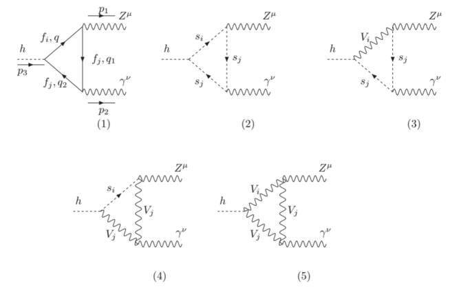
Figure 1: One-loop three-point Feynman diagrams contributing to the decay $h\rightarrow\,Z\gamma$ in the unitary gauge, where $f_{i,j}$ are the SM leptons, $s_{i,j}=H^{\pm},H^{\pm A},H^{\pm B}$, $v_{i,j}=W^{\pm},Y^{\pm A},V^{\pm B}$.

The partial decay width is Gunion:1989we ; Degrande:2017naf

$$\Gamma(h\rightarrow Z\gamma)=\frac{m_{h}^{3}}{32\pi}\times\left(1-\frac{m_{Z}^{2}}{m_{h}^{2}}\right)^{3}|F_{21}|^{2},$$ (80)

where the scalar factor $F_{21}$ is determined from one-loop contributions. More general formulas were given in Ref. Hue:2017cph , leading the following expression

$$F^{331}_{21} =\sum_{f}F^{331}_{21,f}+\sum_{s}F^{331}_{21,s}+\sum_{v}F^{331}_{21,v}+\sum_{\{s,v\}}\left(F^{331}_{21,vss}+F^{331}_{21,svv}\right).$$ (81)

We note that $F^{331}_{21,vss}$ and $F^{331}_{21,svv}$ were not included in previous works Cao:2016uur ; Yue:2013qba .

The detailed analytic formulas of particular notations in (81) are given in appendix B. The partial decay width of the decay $h\rightarrow\gamma\gamma$ can be calculated as Degrande:2017naf ; Hue:2017cph

$$\Gamma(h\rightarrow\gamma\gamma)=\frac{m_{h}^{3}}{64\pi}\times|F^{331}_{\gamma\gamma}|^{2},$$ (82)

where

$$F^{331}_{\gamma\gamma} =\sum_{f}F^{331}_{\gamma\gamma,f}+\sum_{s}F^{331}_{\gamma\gamma,s}+\sum_{v}F^{331}_{\gamma\gamma,v},$$ (83)

see detailed analytic formulas in appendix B. To determine the Br of a SM-like Higgs decay, we need to know the total decay width. In the SM, this quantity is Heinemeyer:2013tqa ; deFlorian:2016spz

$$\Gamma_{h}^{\mathrm{SM}} =\sum_{q\neq t}\Gamma^{\mathrm{SM}}(h\rightarrow\bar{q}q)+\sum_{\ell=e,\mu\tau}\Gamma^{\mathrm{SM}}(h\rightarrow\ell^{+}\ell^{-})+\Gamma^{\mathrm{SM}}(h\rightarrow WW^{*})+\Gamma^{\mathrm{SM}}(h\rightarrow ZZ^{*})$$

$$+\Gamma^{\mathrm{SM}}(h\rightarrow\gamma\gamma)+\Gamma^{\mathrm{SM}}(h\rightarrow Z\gamma)+\Gamma^{\mathrm{SM}}(h\rightarrow gg),$$ (84)

where the partial decay widths are well-known with Higgs boson mass of 125.09 GeV found experimentally Tanabashi:2018oca . The Br of a particular decay channel $h\rightarrow X$, $X=gg,\gamma\gamma,Z\gamma$, is:

$$\mathrm{Br}^{\mathrm{SM}}(h\rightarrow X)\equiv\frac{\Gamma^{\mathrm{SM}}(h\rightarrow X)}{\Gamma_{h}^{\mathrm{SM}}}.$$ (85)

The numerical values are given in table 7 Heinemeyer:2013tqa ; deFlorian:2016spz , where the diphoton decay is consistent with that used in Ref. Aaboud:2018xdt , Br$(h\rightarrow\gamma\gamma)=(2.27\pm 0.07)\times 10^{-3}$.

$b\bar{b}\;$	$\tau^{+}\tau^{-}$	$\mu^{+}\mu^{-}$	$c\bar{c}\;$	$gg$	$\gamma\gamma$	$Z\gamma$	$WW$	$ZZ$	$\Gamma^{\mathrm{SM}}_{h}$ (GeV)
0.5809	0.06256	$2.171\times 10^{-4}$	$0.02884$	$0.0818$	$0.00227$	$0.001541$	$0.2152$	$0.02641$	$4.10\times 10^{-3}$

Table 7: Branching ratios of the SM Higgs boson decays with mass of 125.09 GeV.

The recent global signal strength found experimentally by ATLAS is $\mu_{\gamma\gamma}=0.99\pm 0.14$ Aaboud:2018xdt .

The total decay width of the SM-like Higgs boson predicted by the $331\beta$ is computed based on the deviations of the Higgs couplings with fermions and gauge bosons between the two models SM and $331\beta$, as given in tables 1 and 3. The result is

$$\Gamma_{h}^{331} =0.6725\left(c_{\delta}-\frac{s_{\delta}}{t_{12}}\right)^{2}\Gamma_{h}^{\mathrm{SM}}$$

$$+c^{2}_{\delta}\left[0.2152+\left(1-\frac{2c_{\theta}s_{\theta}c_{W}}{\sqrt{1-\beta^{2}t_{W}^{2}}}\left(\beta t_{W}^{2}+\frac{s_{12}c_{\alpha}+c_{12}s_{\alpha}}{\sqrt{3}c_{\delta}}\right)\right)^{2}0.02641\right]\Gamma_{h}^{\mathrm{SM}}$$

$$+\Gamma^{331}(h\rightarrow\gamma\gamma)+\Gamma^{331}(h\rightarrow Z\gamma)+\Gamma^{331}(h\rightarrow gg).$$ (86)

There are three loop-induced decays $h\rightarrow\gamma\gamma,Z\gamma,gg$. The SM-like Higgs boson does not couple with the exotic quarks in the $331\beta$, we can consider only the top quark contribution to the loop contributing to the decay $h\rightarrow gg$. This results in

$$\Gamma^{331}(h\rightarrow gg)=\left(c_{\delta}+t_{12}s_{\delta}\right)^{2}\Gamma^{\mathrm{SM}}(h\rightarrow gg),$$ (87)

where the deviation comes from the $ht\bar{t}$ coupling listed in table 1. This is consistent with recent investigation for $h\rightarrow\gamma\gamma$ in a 3-3-1 model CarcamoHernandez:2019vih .

In the 331$\beta$ framework, the branching ratio of the decay $h\rightarrow\,X$ with $X=\gamma\gamma,Z\gamma$ is

$$\mathrm{Br}^{331}(h\rightarrow X)\equiv\frac{\Gamma^{331}(h\rightarrow X)}{\Gamma_{h}^{331}}.$$ (88)

Many experimental measurements relating to the SM-like Higgs boson were reported in Ref. Khachatryan:2016vau . We consider the SM-like Higgs production through the gluon fusion process $ggF$ at LHC. The respective signal strength predicted by $331\beta$ is defined as:

$$\mu^{331}_{ggF}\equiv\frac{\sigma^{331}(gg\rightarrow h)}{\sigma^{\mathrm{SM}}(gg\rightarrow h)}\simeq\left(c_{\delta}+t_{12}s_{\delta}\right)^{2},$$ (89)

where the last value comes from our assumption that only the main contribution from top quark in the loop is considered. The signal strength of an individual loop-induced decay channel is

$$\mu^{331}_{X}\equiv\left(c_{\delta}+t_{12}s_{\delta}\right)^{2}\times\frac{\mathrm{Br}^{331}(h\rightarrow X)}{\mathrm{Br}^{\mathrm{SM}}(h\rightarrow X)}.$$ (90)

The recent signal strengths of the two loop-induced decay $h\rightarrow Z\gamma$ is $\mu_{Z\gamma}<6.6(5.2)$ Aaboud:2017uhw ; Tanabashi:2018oca .

III.3 Decays of the neutral Higgs boson $h^{0}_{3}$

In the above discussion we derived only couplings that contribute to the one-loop amplitudes of the two SM-like Higgs decay channels $h\rightarrow\gamma\gamma,Z\,\gamma$. Other interesting couplings are listed in the appendix A. Here we stress a very interesting property of the heavy neutral Higgs boson $h^{0}_{3}$ that it has only one non-zero coupling with two SM particles, namely only $\lambda_{h^{2}h^{0}_{3}}\neq 0$. We have $m_{h^{0}_{3}}>2m_{h}$ then if $h^{0}_{3}$ is lighter than all other exotic particles predicted by the 331$\beta$ model, only the tree level decay $h^{0}_{3}\rightarrow hh$ appears. Loop-induced decays such as $h^{0}_{3}\rightarrow\,gg,\gamma\gamma,Z\gamma$ also appear, as we will present below. Hence, the total decay width of $h^{0}_{3}$ cannot satisfy the stable condition of a dark matter, $\Gamma_{h^{0}_{3}}<1.3\times 2\pi\times 10^{-42}$ GeV Banerjee:2016vrp ; DeLopeAmigo:2009dc ; Eiteneuer:2017hoh ; Belyaev:2016lok . Anyway, DM candidates as scalar 3-3-1 Higgs bosons were pointed out previously Filippi:2005mt ; Cogollo:2014jia ; deS.Pires:2007gi .

The couplings of neutral heavy Higgs bosons $h^{0}_{2,3}$ to fermions are

$$Y_{h^{0}_{2}ffL,R} =\begin{cases}\frac{m_{f}}{v}\left(\frac{c_{\delta}}{t_{12}}+s_{\delta}\right),~{}&f=e_{a},u_{i},d_{3}\\ \frac{m_{f}}{v}\left(-c_{\delta}t_{12}+s_{\delta}\right),~{}&f=u_{3},d_{i}\\ 0,&~{}f=E_{a},J_{a}.\end{cases},\quad Y_{h^{0}_{3}ffL,R}=\begin{cases}0&f=e_{a},u_{a},d_{a}\\ \frac{m_{f}}{v_{3}}&f=E_{a},J_{a}\end{cases}.$$ (91)

One interesting point is that $h^{0}_{3}$ couples to only exotic fermions, similar to the heavy neutral Higgs appeared in a $SU(2)_{1}\times SU(2)_{2}\times U(1)_{Y}$ model Boucenna:2016qad , where the partial decay width $h^{0}_{3}\rightarrow\,gg$ is  Gunion:1989we ; Spira:1997dg ,

$$\Gamma(h^{0}_{3}\rightarrow\,gg)\simeq\frac{\alpha_{s}^{2}m^{3}_{h^{0}_{3}}}{32\pi^{3}v_{3}^{2}}\left|\sum_{a=1}^{3}t_{a}\left[1+(1-t_{a})f(t_{a})\right]\right|^{2},$$ (92)

where $t_{a}\equiv 4m^{2}_{J_{a}}/m^{2}_{h^{0}_{3}}$,

$$f(x) =\begin{cases}\mathrm{arcsin}^{2}\frac{1}{\sqrt{x}},&x\geq 1\\ -\frac{1}{4}\left[\ln\frac{1+\sqrt{1-x}}{1-\sqrt{1-x}}-i\pi\right]^{2},&x<1.\\ \end{cases}$$ (93)

In the limit $t_{a}\gg 1~{}\forall a=1,2,3$, Eq. (92) can be estimated as Boucenna:2016qad

$$\Gamma(h^{0}_{3}\rightarrow\,gg)\simeq\frac{\alpha_{s}^{2}m^{3}_{h^{0}_{3}}}{8\pi^{3}v_{3}^{2}}.$$ (94)

Furthermore, the production cross section of this Higgs boson through the gluon-gluon fusion can be estimated from the two gluon decay channel Boucenna:2016qad .

The partial width of the tree level decay $h^{0}_{3}\rightarrow hh$ when $m_{h^{0}_{3}}>2m_{h}$ is Okada:2016whh

$$\Gamma(h^{0}_{3}\rightarrow hh) =\frac{|\lambda_{h^{0}_{3}hh}|^{2}}{8\pi\,m_{h^{0}_{3}}}\sqrt{1-\frac{4m^{2}_{h}}{m^{2}_{h^{0}_{3}}}}=\frac{\lambda_{13}^{2}s^{4}_{\delta}v_{3}^{2}}{8\pi\,c^{4}_{12}\,m_{h^{0}_{3}}}\sqrt{1-\frac{4m^{2}_{h}}{m^{2}_{h^{0}_{3}}}},$$ (95)

where $\lambda_{13}$ was given in Eq. (73).

The total decay width of the $h^{0}_{3}$ is then

$$\Gamma_{h^{0}_{3}}=\Gamma(h^{0}_{3}\rightarrow\,hh)+\Gamma(h^{0}_{3}\rightarrow gg)+\Gamma(h^{0}_{3}\rightarrow\,\gamma\gamma)+\Gamma(h^{0}_{3}\rightarrow\,Z\gamma).$$ (96)

The last two decays are calculated as follows,

$$\Gamma(h^{0}_{3}\rightarrow Z\gamma) =\frac{m_{h^{0}_{3}}^{3}}{32\pi}\left(1-\frac{m_{Z}^{2}}{m_{h^{0}_{3}}^{2}}\right)^{3}|F_{21}(h^{0}_{3}\rightarrow\,Z\gamma)|^{2},$$ (97)

$$\Gamma(h^{0}_{3}\rightarrow\gamma\gamma) =\frac{m_{h^{0}_{3}}^{3}}{64\pi}\times|F^{331}_{\gamma\gamma}(h^{0}_{3}\rightarrow\gamma\gamma)|^{2},$$ (98)

where

$$F^{331}_{21}(h^{0}_{3}\rightarrow\,Z\gamma) =\sum_{F=E_{a},J_{a}}F^{331}_{21,F}(h^{0}_{3}\rightarrow\,Z\gamma)+\sum_{s}F^{331}_{21,s}(h^{0}_{3}\rightarrow\,Z\gamma)+\sum_{v=Y,V}F^{331}_{21,v}(h^{0}_{3}\rightarrow\,Z\gamma)$$

$$+\sum_{\{s,v\}}\left[F^{331}_{21,vss}(h^{0}_{3}\rightarrow\,Z\gamma)+F^{331}_{21,svv}(h^{0}_{3}\rightarrow\,Z\gamma)\right],$$ (99)

$$F^{331}_{\gamma\gamma}(h^{0}_{3}\rightarrow\,\gamma\gamma) =\sum_{F=E_{a},J_{a}}F^{331}_{\gamma\gamma,F}(h^{0}_{3}\rightarrow\,Z\gamma)+\sum_{s}F^{331}_{\gamma\gamma,s}(h^{0}_{3}\rightarrow\,Z\gamma)+\sum_{v=Y,V}F^{331}_{\gamma\gamma,v}(h^{0}_{3}\rightarrow\,Z\gamma),$$

where $s=H^{\pm},H^{\pm,A},H^{\pm,B}$, $v=Y^{\pm,A},V^{\pm,B}$, and $\{s,v\}=\{H^{\pm,A},Y^{\pm,A}\},\{H^{\pm,B},V^{\pm,B}\}$. The explicit forms in (99) were shown in appendix B.

IV Numerical discussions

IV.1 Signal of the decay $h\rightarrow Z\gamma$ under recent constraints of parameters and the decay $h\rightarrow\gamma\gamma$

In this section, to express quantitative deviations between predictions of the two models 331$\beta$ and the SM for decays $h\rightarrow X$ ($X=\gamma\gamma,Z\gamma$), we define a quantity $\delta\mu_{X}$ as follows

$$\delta{\mu}_{X}\equiv\left(\mu^{331}_{X}-1\right)\times 100\%.$$ (100)

We also introduce a new quantity $R_{Z\gamma/\gamma\gamma}\equiv|\delta\mu_{Z\gamma}/\delta\mu_{\gamma\gamma}|$ to investigate the relative difference between the two signal strengths, which have many similar properties. The recent allowed values relating with the two photon decay is $-15\%\leq\delta\mu_{\gamma\gamma}\leq 13\%$, corresponding to the recent experimental constraint $\mu_{\gamma\gamma}=0.99\pm 0.14$ Aaboud:2018xdt . The future sensitivities obtained by experiments we accept here are $\mu_{\gamma\gamma}=1\pm 0.04$ and $\mu_{Z\gamma}=1\pm 0.23$ Cepeda:2019klc , i.e. $|\delta\mu_{\gamma\gamma}|\leq 4\%$ and $|\delta\mu_{Z\gamma}|\leq 23\%$, respectively.

Many well-known quantities used in this section are fixed from experiments Tanabashi:2018oca , namely the SM-like Higgs mass $m_{h}=125.09$ GeV; the gauge boson masses $m_{W}$, $m_{Z}$; well-known charged fermion masses; the vev $v\simeq 246$ GeV; and the $SU(2)_{L}$ couplings $g\simeq 0.651$, $\alpha_{\mathrm{em}}=1/137$, $e=\sqrt{4\pi\alpha_{\mathrm{em}}}$, $s^{2}_{W}=0.231$.

The unknown independent parameters used as inputs are $\beta$, $t_{12}$, $SU(3)_{L}$ scale $v_{3}$, the neutral Higgs mixing $s_{\delta}$, the heavy neutral Higgs boson masses $m_{h^{0}_{2}}$, $m_{h^{0}_{3}}$, the triple Higgs self couplings including $\lambda_{1}$, $\tilde{\lambda}_{12}$, $\tilde{\lambda}_{13}$, $\tilde{\lambda}_{23}$, and the exotic fermion masses $m_{E_{a}}$, $m_{J_{a}}$.

The exotic fermion masses $m_{E_{a}}$, $m_{J_{a}}$ affect only the loop-induced decays of $h^{0}_{3}$. We can put $m_{E_{a}}=m_{J_{a}}=m_{F}$ for simplicity. There is a more general case that the mixing between different exotic leptons appear, then the loop with two distinguished fermions will contribute to the $h^{0}_{3}\rightarrow\,Z\gamma$ decay amplitude only.

The $SU(3)_{L}$ scale depends strongly on the heavy neutral gauge boson mass $m_{Z^{\prime}}$, which the lower bound is constrained from experimental searches for decays to pairs of SM leptons $Z^{\prime}\rightarrow\ell\bar{\ell}$, for 3-3-1 models see Coutinho:2013lta , where decays into exotic lepton pairs were included. Accordingly, at LHC@14TeV, $m_{Z^{\prime}}<4$ TeV is excluded at the integrated luminosity of $23~{}\mathrm{fb}^{-1}$ for $\beta=-1/\sqrt{3}$. Recent works have used the $m_{Z^{\prime}}\geq 4$ TeV for models with $\beta=-1/\sqrt{3}$ Ferreira:2019qpf ; Long:2018dun , based on the latest LHC search Aaboud:2017sjh ; Sirunyan:2018exx ; Aad:2019fac . Because $v_{3}\sim\mathcal{O}(1)$ TeV, the $m_{Z^{\prime}}$ is approximately calculated from $m_{Z^{\prime}}^{2}=\frac{g^{2}v_{3}^{2}c^{2}_{W}}{3[1-(1+\beta^{2})s^{2}_{W}]}$. From this, the lower bound of $m_{Z^{\prime}}>4$ TeV corresponds to lower bounds of $v_{3}\geq 10.6,\,10.1,\,8.2,\,3.3$ TeV with respective values of $\beta=0,\pm 1/\sqrt{3},\pm 2/\sqrt{3},\pm\sqrt{3}$. Recent discussion on 3-3-1 models with heavy right-handed neutrinos where $\beta=-1/\sqrt{3}$ and $m_{Z^{\prime}}=3$ TeV is allowed Freitas:2018vnt ; Arcadi:2019uif because the decay of $Z^{\prime}$ into a pair of light exotic neutrinos is included. The respective lower bound of the $SU(3)_{L}$ scale is $v_{3}\geq 7.6$ TeV, which is still the same mentioned bounds. On the other hand, a model with $\beta=\sqrt{3}$ still allows rather low $SU(3)_{L}$ scale, for example $m_{Z^{\prime}}\simeq 3.25$ TeV, corresponding to $v_{3}\simeq 2.7$ TeV Coriano:2018coq . Because the numerical results do not change significantly in the range $7.6\;\mathrm{TeV}<v_{3}<14$ TeV, we will fixed $v=14$ TeV for $|\beta|<\sqrt{3}$ and $v=3$ TeV for $|\beta|=\sqrt{3}$.

The perturbative limits require that the absolute values of all Yukawa and Higgs self-couplings should be less than $\sqrt{4\pi}$ and $4\pi$, respectively. This leads to an upper bound of $t_{12}$ derived from the Yukawa coupling of the top quark in Eq. (29), namely $t_{12}<\sqrt{2\pi}v/m_{t}\simeq 3.5$. Other studies on the 2HDM suggest that $t_{12}>1/60$ Cepeda:2019klc . We will limit that $0.1\leq\,t_{12}\leq 3$, which is consistent with Ref. Okada:2016whh and allows large $|s_{\theta}|\geq 5\times 10^{-3}$.

Considering $m_{h^{0}_{2}},m_{A},m_{H^{\pm}}$, $t_{12}$ and $s_{\delta}$ as parameters of a 2HDM model mentioned in Ref. Kanemura:2018yai , an important constraint can be found as $c_{\delta}>0.99$ for all 2HDMs, leading to rather large range of $|s_{\delta}|<0.14$. But large $s_{\delta}$ prefers that $t_{12}$ is around 1 Aad:2015pla . The recent global fit for 2HDM gives the same result Haller:2018nnx . Lower masses of heavy Higgs bosons are around 1 TeV. As we will show, the recent signal strength of the SM-like Higgs decay $h\rightarrow\gamma\gamma$ gives more strict constraint on $s_{\theta}$, hence we focus on the interesting range $|s_{\theta}|\leq 0.05$. The parameters $\lambda_{2}$ and $\lambda_{12}$ relating with 2HDM affect strongly on $m_{h^{0}_{2}}$. Large $|s_{\theta}|$ results in small allowed values of $m_{h^{0}_{2}}$ in order to keep $\lambda_{12}$ satisfying the perturbative limit. In contrast, all other quantities relating with the $SU(3)_{L}$ symmetry are well allowed. The regions of parameter space chosen here are consistent with the recent works on 2HDM Ferreira:2019iqb ; Kainulainen:2019kyp ; Babu:2018uik . The recent experimental searches for Higgs bosons predicted by 2HDM have been paid much attentions Aaboud:2017gsl . The value of 300 GeV for lower bounds of charged and $CP$-even neutral Higgs bosons are accepted in recent studies on 2HDM Babu:2018uik . Following that, values of $m_{h^{0}_{2}}$ and $m_{H^{\pm}}$ will be chosen to satisfy $m_{h^{0}_{2}},m_{H^{\pm}}\geq 300$ GeV.

We will also consider the case of light charged Higgs masses, which loop contributions to the decay $h\rightarrow\gamma\gamma,Z\gamma$ may be large. Accordingly, the Higgs self-couplings $\tilde{\lambda}_{ij}$ relating with charged Higgs masses in Eqs. (49), (54) and (59), should be negative. Our investigation suggests that $|\tilde{\lambda}_{13,23}|\leq\mathcal{O}(10^{-3})$ while $|\tilde{\lambda}_{12}|$ can be reach order 1. We will consider more detailed in particular numerical investigations.

Strict constraints of the Higgs self-couplings for a 3-3-1 model with right handed neutrino were discussed in Ref. Sanchez-Vega:2018qje , where the Higgs potential is forced to satisfy the vacuum stability condition. Accordingly, interesting results can be applied to the 3-3-1 models with arbitrary $\beta$, namely

$$\lambda_{i}>0,\quad f_{ij}\equiv\lambda_{ij}+2\sqrt{\lambda_{i}\lambda_{j}} >0,\quad\tilde{f}_{ij}\equiv\lambda_{ij}+\tilde{\lambda}_{ij}+2\sqrt{\lambda_{i}\lambda_{j}}>0,$$ (101)

with $i,j=1,2,3$ and $i<j$. Note that the constraints on the Higgs self-couplings $\lambda_{1,2,12}$ correspond to the particular cases of the 2HDM Tanabashi:2018oca ; Kanemura:2018yai ; Kanemura:1999xf . Because $\left(t_{12}+t^{-1}_{12}+c_{12}(v/v_{3})^{2}\right)fv_{3}\sim m_{A}^{2}$ being the squared mass of the $CP$-odd neutral Higgs boson, the requirement $m^{2}_{A}>0$ shows $f>0$ Okada:2016whh ; Dias:2009au . The other conditions guarantee that all squared Higgs masses must be positive and SM-like Higgs mass is identified with the experimental value. It can be seen in Eqs. (49)-(59) that all charged Higgs squared masses are always positive if all $\tilde{\lambda}_{ij}>0$, but their values seem very large. More interesting cases correspond to the existence of light charged Higgs bosons, which may contribute significant contributions to loop-induced decays of the SM-like Higgs bosons. Based on eq. (61), a first estimation suggests that $f$ has the same order with $SU(3)_{L}$ scale $v_{3}$, leading to the requirement that $\tilde{\lambda}_{12,13,23}<0$ for the existence of light charged Higgs bosons. Furthermore, the relation (73) results in a consequence that $\lambda_{13}$ will be small for the case of our interest with large $v_{3}\geq 3$ TeV and small $m_{h^{0}_{2}}$ around 1 TeV. In this case $f$ is also small, as we realize in the numerical investigation as well as it has been shown recently Palcu:2019nld . Taking this into account to the charged Higgs masses in Eqs.(54) and (59) we derive that the absolute values of negative values of $\tilde{\lambda}_{13,23}$ seems very small. In contrast, the appearance of a light charged Higgs $H^{\pm}$ allows negative $\tilde{\lambda}_{12}$ and rather large $|\tilde{\lambda}_{12}|$ that satisfy the inequality $\tilde{f}_{12}>0$ given in (101). We will consider the two separate cases: $\tilde{\lambda}_{ij}\geq 0$ with all $i>j$, $i,j=1,2,3$; and $\tilde{\lambda}_{12}<0$. The values of $\lambda_{13,23}$ are always chosen to get large absolute values of $F^{331}_{21,s}$, and/or $F^{331}_{21,sv}\equiv F^{331}_{21,svv}+F^{331}_{21,vss}$.

The above discussion allows us to choose the default values of unknown independent parameters as follows: $\beta=1/\sqrt{3}$, $s_{\delta}=0.01$, $\lambda_{1}=1$, $t_{12}=0.8$, $\tilde{\lambda}_{12}=\tilde{\lambda}_{13}=\tilde{\lambda}_{23}=0.1$, $m_{h^{0}_{2}}=1.2$ TeV, $m_{h^{0}_{3}}=1$ TeV, $v_{3}=14$ TeV, $m_{E_{a}}=m_{J_{a}}=1.5$ TeV. We choose the perturbative limit of Higgs self-couplings is $10$, which is a bit more strict than $4\pi$ . In addition, depending on the particular discussions, changing any numerical values will be noted.

IV.1.1 Case 1: $\tilde{\lambda}_{12}\geq 0$

First, we focus on the 2HDM parameters. Fig. 2 and 3 illustrate numerically Higgs self-couplings and $f_{ij}$ as functions of $m_{h^{0}_{2}}$, and other independent parameters are fixed as $t_{12}=0.8$ and changing $s_{\delta}=\pm 10^{-2},\pm 5\times 10^{-2}$, which are significantly large.

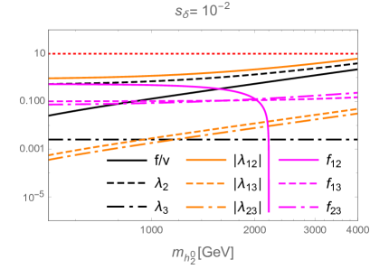
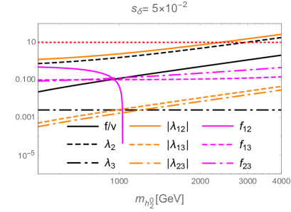
Figure 2: $f_{ij}$ and Higgs self-couplings as functions of $m_{h^{0}_{2}}$ with $s_{\delta}>0$ and $t_{12}=0.8$. The horizontal lines at the value of $10$ correspond to the perturbative limit of the Higgs self-couplings.

For $s_{\delta}>0$, the $t_{12}$ is chosen large enough to satisfy $f_{12}>0$ and $m_{h^{0}_{2}}>1$ TeV. The parameters $\tilde{\lambda}_{12}\geq 0$ and negative $\tilde{\lambda}_{13,23}\rightarrow 0$ do not affect the quantities investigated in this figure. We conclude that the vacuum stability requirement $f_{12}>0$ gives strong upper bound on $m_{h^{0}_{2}}$, where larger $s_{\delta}$ gives smaller allowed $m_{h^{0}_{2}}$.

Fig.  3 illustrates allowed regions for $s_{\delta}<0$, where we choose $t_{12}=0.1$, enough small to allow $\lambda_{2}>0$ and $m_{h^{0}_{2}}>1$ TeV.

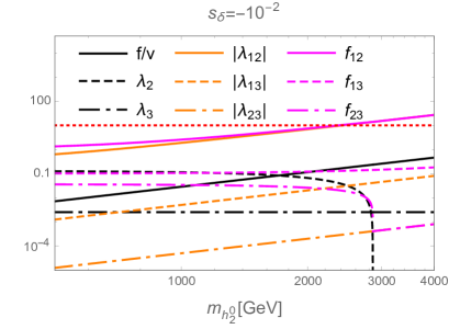
Figure 3: $f_{ij}$ and Higgs self-couplings as functions of $m_{h^{0}_{2}}$ with $s_{\delta}<0$ and $t_{12}=0.1$.

Again we derive that larger $|s_{\delta}|$ gives smaller upper bound of $m_{h^{0}_{2}}$.

In general, our scan shows that allowed $t_{12}$ and $s_{\theta}$ are affected the most strongly by $m_{h^{0}_{2}}$. As illustration, the Fig. 4 presents allowed regions of $t_{12}$ and $s_{\theta}$ with two fixed $m_{h^{0}_{2}}=1$ TeV and $2.5$ TeV.

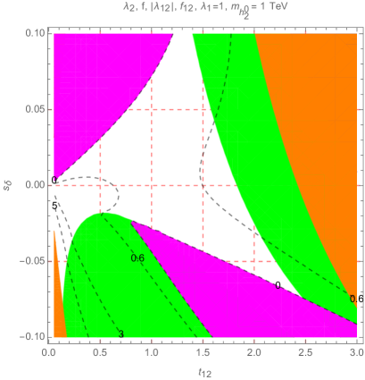
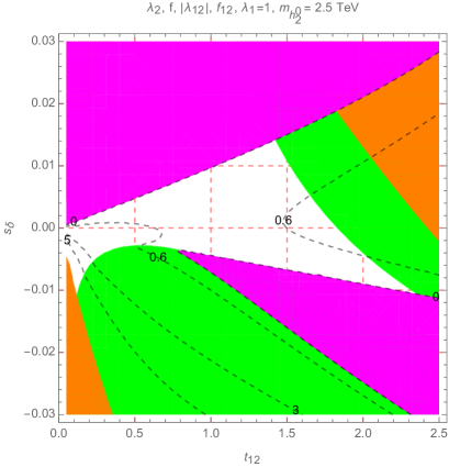
Figure 4: Contour plots of $\lambda_{2}$, $f$, $|\lambda_{12}|$ and $f_{12}$ as functions of $s_{\theta}$ and $t_{12}$. The green, blue, orange, magenta regions are excluded by requirements that $0<\lambda_{2}<10$, $f>0$, $|\lambda_{12}|<10$, and $f_{12}>0$, respectively. Dashed-black curves present constant values of $f_{12}$.

It can be seen that larger $m_{h^{0}_{2}}$ results in smaller allowed $|s_{\theta}|$. The dashed black curves presenting constant values of $f_{12}$ will be helpful for the discussion on the case of $\tilde{\lambda}_{12}<0$. This is because the constraint from $\tilde{f}_{12}>0$ will be more strict than that from $f_{12}>0$ when $\tilde{\lambda}_{12}<0$, namely it will be equivalent to $f_{12}>|\tilde{\lambda}_{12}|$. Hence $f_{12}$ plays role as the upper bound of $|\tilde{\lambda}_{12}|$.

The allowed regions also depend on $\lambda_{1}$, see contour plots in Fig. 5 corresponding to $\lambda_{1}=0.5,5$.

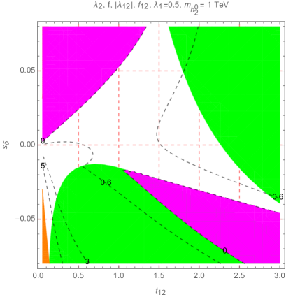
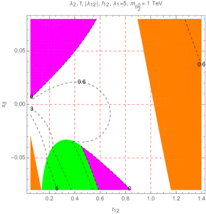
Figure 5: Contour plots of $\lambda_{2}$, $|\lambda_{12}|$ and $f_{12}$ as functions of $s_{\delta}$ and $t_{12}$. The green, blue, orange, magenta regions are excluded by requirements that $0<\lambda_{2}<10$, $f>0$, $|\lambda_{12}|<10$, and $f_{12}>0$, respectively. Dashed-black curves presents constant values of $f_{12}$.

It can be seen that $\lambda_{1}$ should be large enough to allow large $|s_{\theta}|$, see illustrations in Fig. 12 for $\lambda_{1}=0.1,10$ in appendix C.

In the case of large $|s_{\theta}|=0.02$, the allowed values $\lambda_{1}$ and $t_{12}$ are shown in Fig. 6.

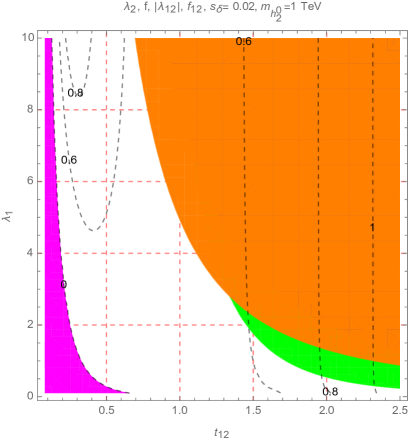
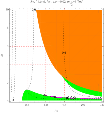
Figure 6: Contour plots of $\lambda_{2}$, $|\lambda_{12}|$ and $f_{12}$ as functions of $\lambda_{1}$ and $t_{12}$ with some fixed $m_{h^{0}_{2}}$ . The green, blue, orange, magenta regions are excluded by requirements that $0<\lambda_{2}<10$, $f>0$, $|\lambda_{12}|<10$, and $f_{12}>0$, respectively. Dashed-black curves present constant values of $f_{12}$.

It can be seen that only negative $s_{\theta}$ allows large $f_{12}$. The case of larger $|s_{\theta}|=0.05$ is shown in Fig. 13 of the appendix C. We can choose $m_{h^{0}_{2}}=1.2$ TeV so that $|s_{\theta}|=0.05$ is still allowed. Both large $|s_{\delta}|$ and $m_{h^{0}_{2}}$ give narrow allowed regions of $t_{12}$ and $\lambda_{1}$, and small $f_{12}$. For small $|s_{\delta}|<10^{-2}$, the allowed values of $m_{h^{0}_{2}}$ and $t_{12}$ will relax. But it will not result in much deviation from the SM prediction.

The left panel of Fig. 7 illustrates the contour plots with fixed $\beta=-1/\sqrt{3}$ for allowed values of $\delta\mu_{Z\gamma}$ corresponding to the noncolored✿ regions that satisfy the constraints of parameters and the recent experimental bound on $\delta\mu_{\gamma\gamma}$.

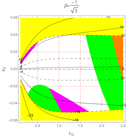
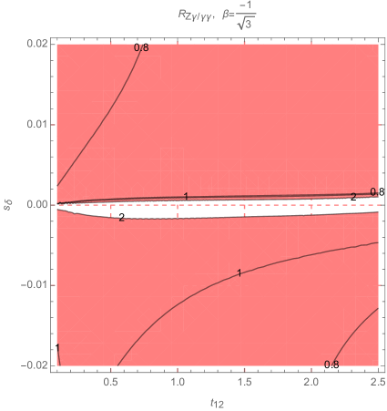
Figure 7: Contour plots showing allowed regions of $s_{\delta}$ and $t_{12}$ (left) and $R_{Z\gamma/\gamma\gamma}$ as a function of $s_{\delta}$ and $t_{12}$. The green, blue, orange, magenta and yellow regions are excluded by valid requirements of $\lambda_{2},f,\lambda_{12},f_{12}$, and $\delta\mu_{\gamma\gamma}$, respectively. The black and dotted black curves show constant values of $\delta\mu_{Z\gamma}$ and $\delta\mu_{\gamma\gamma}$, respectively. The non color region in the right panel corresponds to $R_{Z\gamma/\gamma\gamma}\geq 2$.

The right panel of Fig. 7 shows the contour plots of $R_{Z\gamma/\gamma\gamma}$, where the noncolored region satisfies $R_{Z\gamma/\gamma\gamma}\geq 2$. In this region, we can see that $|s_{\delta}|\sim\mathcal{O}(10^{-3})$ and negative. In addition, $\delta\mu_{\gamma\gamma}<0.04$. Hence, the current constraints $\mu_{\gamma\gamma}=0.99\pm 0.14$ predicts $|\delta\mu_{Z\gamma}|<0.15$ which is still smaller than the future sensitivity $\delta\mu_{Z\gamma}=\pm 0.23$ mentioned in Ref. Cepeda:2019klc . In addition, most of the allowed regions satisfy $0.8\leq\;R_{Z\gamma/\gamma\gamma}\leq\;2$, hence the approximation Br$(h\rightarrow\gamma\gamma)\simeq\mathrm{Br}(h\rightarrow\;Z\gamma)$ is accepted for simplicity in previous works.

For large $v_{3}=14$ TeV and recent uncertainty of the $\delta\mu_{\gamma\gamma}$, our investigation shows generally that the above discussions on the allowed regions as well as $R_{Z\gamma/\gamma\gamma}$ illustrated in Fig. 7 depend weakly on $\beta$. The results are also unchanged for lower bound of $v_{3}=8$ TeV which is allowed for $\beta=\pm 2/\sqrt{3}$. This property can be explained by the fact that, large $v_{3}\simeq 10$ TeV results in heavy charged gauge bosons $m_{Y},m_{V}$ having masses around 4 TeV, and the charged Higgs masses being not less than 1 TeV. As a by-product, one loop contributions from $SU(3)_{L}$ particles to $F^{331}_{21}$ and $F^{331}_{\gamma\gamma}$ are at least four orders smaller than the corresponding SM amplitudes $F^{\mathrm{SM}}_{21,\gamma\gamma}$, illustrations are given in table 8.

$\beta$	$s_{\delta}$	$t_{12}$	$\frac{F^{331}_{21,s}}{\mathrm{Re}[F^{\mathrm{SM}}_{21}]}$	$\frac{F^{331}_{21,v}}{\mathrm{Re}[F^{\mathrm{SM}}_{21}]}$	$\frac{F^{331}_{21,sv}}{\mathrm{Re}[F^{\mathrm{SM}}_{21}]}$	$\frac{F^{331}_{\gamma\gamma,s}}{\mathrm{Re}[F^{\mathrm{SM}}_{\gamma\gamma}]}$	$\frac{F^{331}_{\gamma\gamma,v}}{\mathrm{Re}[F^{\mathrm{SM}}_{\gamma\gamma}]}$	$\delta\mu_{Z\gamma}$	$\delta\mu_{\gamma\gamma}$
$\frac{2}{\sqrt{3}}$	$2\times 10^{-2}$	$1.5$	$-3.3\times 10^{-4}$	$3\times 10^{-5}$	$-1.6\times 10^{-4}$	$-6\times 10^{-4}$	$5.5\times 10^{-4}$	$4.4$	$6.5$
$\frac{2}{\sqrt{3}}$	$-2\times 10^{-2}$	$1.5$	$\sim 10^{-6}$	$3\times 10^{-5}$	$-1.5\times 10^{-4}$	$\sim 10^{-6}$	$5.3\times 10^{-4}$	$-5.4$	$-6$
$\frac{2}{\sqrt{3}}$	$2\times 10^{-2}$	$0.5$	$1.3\times 10^{-4}$	$-9\times 10^{-5}$	$-5\times 10^{-5}$	$2.3\times 10^{-4}$	$2.2\times 10^{-4}$	$6.8$	$8.1$
$\frac{2}{\sqrt{3}}$	$-2\times 10^{-2}$	$0.5$	$-4.2\times 10^{-4}$	$-9\times 10^{-5}$	$-4\times 10^{-5}$	$-7.5\times 10^{-4}$	$2.1\times 10^{-4}$	$-7.5$	$-7.4$
$\frac{2}{\sqrt{3}}$	$-10^{-3}$	$1.5$	$-1.6\times 10^{-4}$	$3\times 10^{-5}$	$-1.6\times 10^{-4}$	$-2.9\times 10^{-4}$	$5.4\times 10^{-4}$	$-0.8$	$-0.2$

Table 8: Numerical contributions of $SU(3)_{L}$ particles to $F^{331}_{21}$ and $F^{331}_{\gamma\gamma}$, see Eqs. (81) and  (83), where $F^{331}_{21,sv}\equiv F^{331}_{21,svv}+F^{331}_{21,vss}$.

Here we use the SM amplitudes predicted by the SM, namely $\mathrm{Re}[F^{\mathrm{SM}}_{21}]=-5.6\times 10^{-5}\,[\mathrm{GeV}^{-1}]$ and $\mathrm{Re}[F^{\mathrm{SM}}_{\gamma\gamma}]=-3.09\times 10^{-5}\,[\mathrm{GeV}^{-1}]$, and ignore the tiny imaginary parts. We can see that both $\delta\mu_{Z\gamma}$ and $\delta\mu_{\gamma\gamma}$ depend strongly on $s_{\delta}$ and $t_{12}$. In contrast, the one-loop contributions from new particles are suppressed, as shown in the last line in table 8: suppressed $s_{\delta}$ results in $|\delta\mu_{Z\gamma}|\simeq 4|\delta\mu_{\gamma\gamma}|=0.8\%\ll 4\%$, which is even much smaller than the expected sensitivity of $\delta\mu_{\gamma\gamma}=4\%$. Anyway, it can be noted that $F^{331}_{21,sv}$ may significantly larger than $F^{331}_{21,v}$, hence both of them should be included simultaneously into the decay amplitude $h\rightarrow\;Z\gamma$ in general. Suppressed contributions of new particles to $\delta\mu_{Z\gamma,}$ are shown explicitly in the left panel of Fig. 7, where three constant curves $s_{\delta}=\delta\mu_{Z\gamma}=\delta\mu_{\gamma\gamma}=0$ are very close together.

For large and positive $\tilde{\lambda}_{12}$ and small $m_{h^{0}_{2}}$, one loop contributions from $H^{\pm}$ to $F^{331}_{21}$ and $F^{331}_{\gamma\gamma}$ are dominant but still not large enough to give significant deviations to $\delta\mu_{Z\gamma}$, see an illustration with suppressed $s_{\delta}=10^{-3}$ in the first line of table 9.

$\beta$	$s_{\delta}$	$t_{12}$	$\frac{F^{331}_{21,s}}{\mathrm{Re}[F^{\mathrm{SM}}_{21}]}$	$\frac{F^{331}_{21,v}}{\mathrm{Re}[F^{\mathrm{SM}}_{21}]}$	$\frac{F^{331}_{21,sv}}{\mathrm{Re}[F^{\mathrm{SM}}_{21}]}$	$\frac{F^{331}_{\gamma\gamma,s}}{\mathrm{Re}[F^{\mathrm{SM}}_{\gamma\gamma}]}$	$\frac{F^{331}_{\gamma\gamma,v}}{\mathrm{Re}[F^{\mathrm{SM}}_{\gamma\gamma}]}$	$\delta\mu_{Z\gamma}$	$\delta\mu_{\gamma\gamma}$
$\frac{2}{\sqrt{3}}$	$10^{-3}$	$1.7$	$-1.46\times 10^{-2}$	$4\times 10^{-5}$	$-1.7\times 10^{-4}$	$-2.64\times 10^{-2}$	$5.7\times 10^{-4}$	$-3.1$	$-4.7$
$\frac{2}{\sqrt{3}}$	$-10^{-3}$	$1.7$	$-1.44\times 10^{-2}$	$4\times 10^{-5}$	$-1.7\times 10^{-4}$	$-2.61\times 10^{-2}$	$5.7\times 10^{-4}$	$-3.6$	$-5.3$
$\frac{2}{\sqrt{3}}$	$3\times 10^{-2}$	$1.5$	$-1.24\times 10^{-2}$	$3\times 10^{-5}$	$-1.6\times 10^{-4}$	$-2.23\times 10^{-2}$	$5.5\times 10^{-4}$	$4.4$	$5.2$
$\frac{2}{\sqrt{3}}$	$-3\times 10^{-2}$	$1.5$	$-9.6\times 10^{-3}$	$3\times 10^{-5}$	$-1.5\times 10^{-4}$	$-1.75\times 10^{-3}$	$5.3\times 10^{-4}$	$-9.6$	$-12.3$

Table 9: Numerical contributions of $SU(3)_{L}$ particles to $F^{331}_{21}$ and $F^{331}_{\gamma\gamma}$ for large $\tilde{\lambda}_{12}=5$ and small $m_{h^{0}_{2}}=600$ GeV.

Here we always force $|\delta\mu_{\gamma\gamma}|\leq 4\%$ being the future sensitive of $\mu_{\gamma\gamma}$. On the other hand, large deviations can result from large $|s_{\delta}|$. In this case, all $\delta\mu_{Z\gamma,\gamma\gamma}$ and $s_{\delta}$ have the same signs.

Regarding $\beta=\sqrt{3}$ corresponding to the model discussed in Ref. Coriano:2018coq , where $v_{3}=3$ TeV is still accepted, the allowed regions change significantly, as illustrated in Fig. 8.

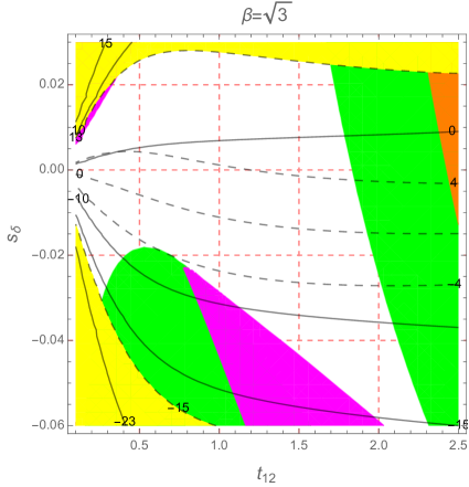
Figure 8: Contour plots showing allowed regions of $s_{\delta}$ and $t_{12}$ with $v_{3}=3$ TeV following Ref. Coriano:2018coq . The green, blue, orange, magenta and yellow regions are excluded by valid requirements of $\lambda_{2},f,\lambda_{12},f_{12}$, and $\delta\mu_{\gamma\gamma}$, respectively. The black and dotted black curves show constant values of $\delta\mu_{Z\gamma}$ and $\delta\mu_{\gamma\gamma}$, respectively.

In particularly, the model gives more strict positive $s_{\delta}<0.03$. One-loop contributions from $SU(3)_{L}$ particles can give deviations up to few percent for both $\delta\mu_{Z\gamma}$, $\delta\mu_{\gamma\gamma}$, as shown in Fig. 8 that the two contours $\delta_{Z\gamma}=\delta\mu_{\gamma\gamma}=0$ distinguish with the line $s_{\delta}=0$. Interesting numerical values are illustrated in table 10.

$\beta$	$s_{\delta}$	$t_{12}$	$\frac{F^{331}_{21,s}}{\mathrm{Re}[F^{\mathrm{SM}}_{21}]}$	$\frac{F^{331}_{21,v}}{\mathrm{Re}[F^{\mathrm{SM}}_{21}]}$	$\frac{F^{331}_{21,sv}}{\mathrm{Re}[F^{\mathrm{SM}}_{21}]}$	$\frac{F^{331}_{\gamma\gamma,s}}{\mathrm{Re}[F^{\mathrm{SM}}_{\gamma\gamma}]}$	$\frac{F^{331}_{\gamma\gamma,v}}{\mathrm{Re}[F^{\mathrm{SM}}_{\gamma\gamma}]}$	$\delta\mu_{Z\gamma}$	$\delta\mu_{\gamma\gamma}$
$\sqrt{3}$	$10^{-3}$	$1.5$	$-1.8\times 10^{-4}$	$-1.6\times 10^{-3}$	$-4\times 10^{-3}$	$-3.2\times 10^{-4}$	$2.2\times 10^{-2}$	$-1.6$	$4.8$
$\sqrt{3}$	$-10^{-3}$	$1.5$	$-1.6\times 10^{-4}$	$-1.7\times 10^{-3}$	$-4\times 10^{-3}$	$-2.9\times 10^{-4}$	$2.2\times 10^{-2}$	$-2$	$4.2$

Table 10: For model in Ref. Coriano:2018coq , numerical contributions of $SU(3)_{L}$ particles to $F^{331}_{21}$ and $F^{331}_{\gamma\gamma}$. Notations are given from caption of table 8.

We emphasize two important properties. First, one loop contributions from gauge $SU(3)_{L}$ bosons are dominant, which can give $\delta\mu_{\gamma\gamma}$ to reach the future sensitivity. Values of $F^{331}_{21,v}$ and $F^{331}_{21,sv}$ can have the same order of $10^{-3}$ compared with the SM part, but these contributions are not large enough to result in large deviation of $|\delta\mu_{Z\gamma}|>23\%$.

To finish the case of $\lambda_{ij}>0$ we mentioned above, we see that in this case all of the charged Higgs boson masses are order of $\mathrm{O}(1)$TeV and they have small couplings with $h$. For large $\lambda_{1}$, $\lambda_{12}$ and small $m_{h^{0}_{2}}=800$ GeV, there may give small $\delta\mu_{\gamma\gamma}$ but large $\delta\mu_{Z\gamma}$, see examples in table 11.

$\lambda_{1}$	$\tilde{\lambda}_{12}$	$s_{\delta}$	$t_{12}$	$\frac{F^{331}_{21,s}}{\mathrm{Re}[F^{\mathrm{SM}}_{21}]}$	$\frac{F^{331}_{21,v}}{\mathrm{Re}[F^{\mathrm{SM}}_{21}]}$	$\frac{F^{331}_{21,sv}}{\mathrm{Re}[F^{\mathrm{SM}}_{21}]}$	$\frac{F^{331}_{\gamma\gamma,s}}{\mathrm{Re}[F^{\mathrm{SM}}_{\gamma\gamma}]}$	$\frac{F^{331}_{\gamma\gamma,v}}{\mathrm{Re}[F^{\mathrm{SM}}_{\gamma\gamma}]}$	$\delta\mu_{Z\gamma}$	$\delta\mu_{\gamma\gamma}$
$1.95$	$8$	$10^{-3}$	$1.5$	$-1.22\times 10^{-2}$	$-1.7\times 10^{-3}$	$-4.4\times 10^{-3}$	$-2.21\times 10^{-2}$	$2.2\times 10^{-2}$	$-4.$	$0.4$
$1.95$	$8$	$-10^{-3}$	$1.5$	$-1.21\times 10^{-2}$	$-1.7\times 10^{-3}$	$-4.4\times 10^{-3}$	$-2.19\times 10^{-2}$	$2.2\times 10^{-2}$	$-4.5$	$-0.17$
$1.$	$5$	$-2\times 10^{-2}$	$1.95$	$-1.6\times 10^{-3}$	$-9.7\times 10^{-4}$	$-5\times 10^{-3}$	$-1.2\times 10^{-2}$	$2.4\times 10^{-2}$	$-7.7$	$-4$

Table 11: For model in Ref. Coriano:2018coq , numerical contributions of $SU(3)_{L}$ particles to $F^{331}_{21}$ and $F^{331}_{\gamma\gamma}$ with $m_{h^{0}_{2}}=800$ GeV. Notations are given from caption of table 8.

We stress here an interesting point that with the existence of new Higgs and gauge bosons, their contributions $F^{331}_{\gamma\gamma,s}$ and $F^{331}_{\gamma\gamma,v}$ to the decay amplitude $h\rightarrow\gamma\gamma$ may be destructive and the same order, hence keep the respective signal strength satisfying the small experimental constraint. Simultaneously, all of the contributions to the decay amplitude $h\rightarrow\,Z\gamma$ are constructive so that the deviation can be large. For the model with $\beta=\sqrt{3}$ and $v_{3}=3$ TeV, we can find this deviation can reach around $-10$, but this values is still far from the expected sensitive $\delta\mu_{Z\gamma}=\pm 23\%$ in the HL-LHC project. For the models with $v_{3}\geq 8$ TeV, heavy gauge contributions are suppressed, hence large contribution from charged Higgs bosons is dominant. Then, the constraint from $\delta\mu_{\gamma\gamma}$ will give more strict constraint on $\delta\mu_{Z\gamma}$ than that obtained from the experiments.

IV.1.2 Case 2: $\tilde{\lambda}_{12}<0$.

As we can see in eq. (49), negative $\tilde{\lambda}_{12}$ may result in small charged Higgs mass $m_{H^{\pm}}$. In addition, large $|\tilde{\lambda}_{12}|$ may give large coupling of this Higgs boson with the SM-like one, leading to large $|F^{331}_{21,s}|$ and $|F^{331}_{\gamma\gamma,s}|$. We will focus on this interesting case.

One of the conditions given in (101), namely $\tilde{f}_{12}>0$, will automatically satisfy if $f_{12}>0$ and $\tilde{\lambda}_{12}\geq 0$. In the case of $\tilde{\lambda}_{12}<0$, the inequality $\tilde{f}_{12}>0$ is equivalent to the more strict condition $f_{12}>|\tilde{\lambda}_{12}|>0$ or $-f_{12}<\tilde{\lambda}_{12}<0$. This helps us determine the allowed regions with large $|\tilde{\lambda}_{12}|$, which give large one-loop contributions of charged Higgs boson $H^{\pm}$ to the two decay amplitudes $h\rightarrow\,Z\gamma,\gamma\gamma$. Based on the fact that allowed regions with large positive $f_{12}$ will allow large $\tilde{\lambda}_{12}$, two Figs. 4 and 5 show that large $\tilde{\lambda}_{12}$ corresponds to regions having negative $s_{\delta}$ and small $t_{12}$. Small $s_{\theta}$ allows small $|\tilde{\lambda}_{12}|$. The Fig. 6 shows that values of $\lambda_{1}$ seems not affect allowed $\tilde{\lambda}_{12}$ in the regions of negative $s_{\delta}$. For large $v_{3}$, large $|\tilde{\lambda}_{12}|$ in this case does not affect significantly on both $\delta\mu_{Z\gamma,\gamma\gamma}$ see illustration in table 12.

$\beta$	$m_{h^{0}_{2}}$ [TeV]	$s_{\delta}$	$\frac{F^{331}_{21,s}}{F^{\mathrm{SM}}_{21}}$	$\frac{F^{331}_{21,v}}{F^{\mathrm{SM}}_{21}}$	$\frac{F^{331}_{21,sv}}{F^{\mathrm{SM}}_{21}}$	$\frac{F^{331}_{\gamma\gamma,s}}{F^{\mathrm{SM}}_{\gamma\gamma}}$	$\frac{F^{331}_{\gamma\gamma,v}}{F^{\mathrm{SM}}_{\gamma\gamma}}$	$\delta\mu_{Z\gamma}$	$\delta\mu_{\gamma\gamma}$
$\frac{2}{\sqrt{3}}$	$1$	$-10^{-3}$	$3.4\times 10^{-4}$	$-1.4\times 10^{-4}$	$\simeq 0$	$6.1\times 10^{-3}$	$9\times 10^{-5}$	$-1.8$	$-1.2$
$\frac{2}{\sqrt{3}}$	$0.6$	$-10^{-3}$	$1.2\times 10^{-3}$	$-1.4\times 10^{-4}$	$\simeq 0$	$-2.1\times 10^{-3}$	$9\times 10^{-5}$	$-1.7$	$-0.9$
$\frac{2}{\sqrt{3}}$	$1$	$-2\times 10^{-2}$	$-1.4\times 10^{-3}$	$-1.4\times 10^{-4}$	$\simeq 0$	$-2.6\times 10^{-3}$	$9\times 10^{-5}$	$-23.9$	$-23.9$
$\frac{2}{\sqrt{3}}$	$0.6$	$-2\times 10^{-2}$	$6.6\times 10^{-4}$	$-1.2\times 10^{-3}$	$\simeq 0$	$-1.2\times 10^{-3}$	$9\times 10^{-5}$	$-23.7$	$-23.6$

Table 12: Numerical contributions of $SU(3)_{L}$ particles to $F^{331}_{21}$ and $F^{331}_{\gamma\gamma}$. Numerical fixed values of unknown parameters are: $\beta=2/\sqrt{3}$, $t_{12}=0.1$, $\tilde{\lambda}_{12}=-1$.

Hence, the case of negative $\tilde{\lambda}_{12}$ may results in light charged Higgs boson $H^{\pm}$, but it does not support large one-loop contributions from charged Higgs mediation to decay amplitudes $h\rightarrow\,Z\gamma,\gamma\gamma$.

Regarding the model with $\beta=\sqrt{3}$ discussed in Ref. Coriano:2018coq , the main difference is the small $v_{3}=3$ TeV, leading to a significant effect of heavy gauge bosons to the one-loop contributions $|F^{331}_{21,v}/F^{\mathrm{SM}}_{21}|,\,|F^{331}_{21,sv}/F^{\mathrm{SM}}_{21}|,\,|F^{331}_{21,s}/F^{\mathrm{SM}}_{21}|,\,|F^{331}_{\gamma\gamma,v}/F^{\mathrm{SM}}_{\gamma\gamma}|,\,|F^{331}_{\gamma\gamma,s}/F^{\mathrm{SM}}_{\gamma\gamma}|\sim\mathcal{O}(10^{-2})$. But with $\tilde{\lambda}_{12}<0$, constructive contributions appear in the decay amplitude $h\rightarrow\gamma\gamma$, while destructive contributions appear in the decay amplitude $h\rightarrow\,Z\gamma$. Hence, the constraint from experimental data of the decay $h\rightarrow\gamma\gamma$ predicts smaller deviation of the $\mu_{Z\gamma}$ than that corresponding to $\tilde{\lambda}_{12}>0$.

To finish, from above discussion we emphasize that in other gauge extensions of the SM such as the $SU(2)_{1}\otimes SU(2)_{2}\otimes U(1)_{Y}$ models, which still allow low values of new gauge and charged Higgs bosons masses Boucenna:2016qad ; Hue:2016nya ; He:2017bft ; Yue:2019kky ; Abdullah:2018ets , the contributions like $F_{12,sv}$ may be as large as usual ones, hence it should be included in the decay amplitude $h\rightarrow\,Z\gamma$. In addition, these models may predict large $\delta\mu_{Z\gamma}$, which also satisfies $|\delta\mu_{\gamma\gamma}|\leq 0.04$. This interesting topic deserves to be paid attention more detailed.

IV.2 $h^{0}_{3}$ decays as a signal of the $331\beta$ model

Different contributions to loop-induced decays $h^{0}_{3}\rightarrow\gamma\gamma,Z\gamma$ with small $s_{\theta}=10^{-3}$, $m_{h^{0}_{3}}=700$ GeV, $t_{12}=0.8$ are illustrated in Fig. 9, where the ratios $|F_{21,x}(h^{0}_{3}\rightarrow\,Z\gamma)|/|F_{21}(h^{0}_{3}\rightarrow\,Z\gamma)|$ and $|F_{\gamma\gamma,x}(h^{0}_{3}\rightarrow\,Z\gamma)|/|F_{\gamma\gamma}(h^{0}_{3}\rightarrow\,Z\gamma)|$ are presented, $x=f,s,v,sv$.

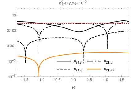
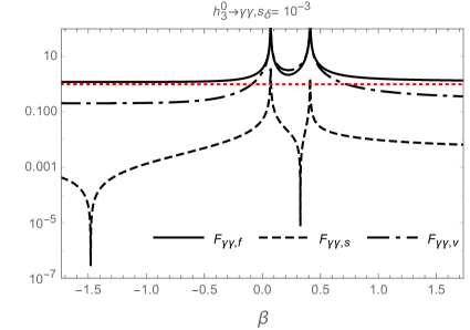
Figure 9: Different contributions to loop-induced decays $h^{0}_{3}\rightarrow\gamma\gamma,Z\gamma$ as functions of $\beta$.

In addition, our scan shows that the curves in the Fig. 9 do not sensitive with the changes of $s_{\delta}$. We can conclude that contributions from heavy exotic fermions are alway dominant for large $\beta$. While $F_{21,sv}$ is suppressed. For the decay $h^{0}_{3}\rightarrow\gamma\gamma$, the destructive correlation between $F_{\gamma\gamma,v}$ and $F_{\gamma\gamma,f}$ happens with small $|\beta|$. This results in two peaks in the figure, where $|F_{\gamma\gamma}|\ll|F_{\gamma\gamma,f}|,|F_{\gamma\gamma,v}|$.

Individual branching ratios of $h^{0}_{3}$ are shown in Fig. 10.

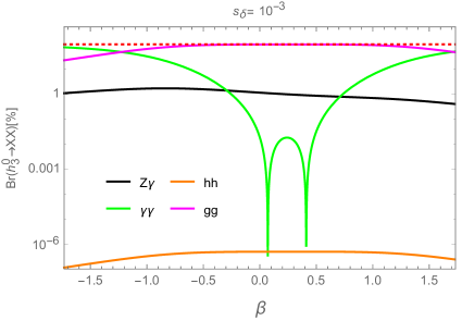
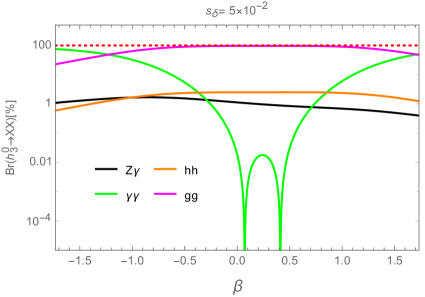
Figure 10: Branching ratios of the $h^{0}_{3}$ decays as functions of $\beta$.

The most interesting property is that, the Br$(h^{0}_{3}\rightarrow\gamma\gamma)$ may have large values and it is very sensitive with the change of $\beta$. Hence this decay is a promising channel to fix the $\beta$ value once $h^{0}_{3}$ exists. On the other hand, Br$(h^{0}_{3}\rightarrow\,hh)$ is sensitive with $s_{\delta}$: it increases significantly with large $s_{\delta}$, but the values is always small Br$(h^{0}_{3}\rightarrow\,hh)<1\%$.

For $m_{F}>m_{h^{0}_{3}}$ the total decay width of the $h^{0}_{3}$ gets dominant contribution from two gluons decay channel, hence it is sensitive with only $m_{h^{0}_{3}}$ and $v_{3}$, as given in Eq. (94). It is a bit sensitive with $\beta$, see illustrations in Fig. 11.

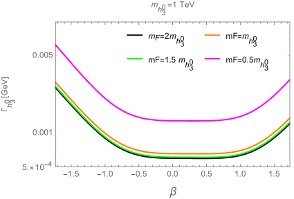
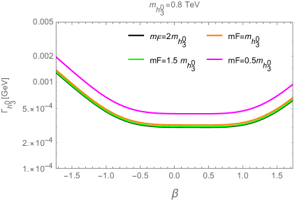
Figure 11: Total decay width of $h^{0}_{3}$ as functions of $\beta$, where decays to exotic particle pairs do not included.

V Conclusions

The signals of new physics predicted by the 3-3-1 models from the loop-induced neutral Higgs decays $h,h^{0}_{3}\rightarrow\gamma\gamma,Z\gamma$ have been discussed. For the general case with arbitrary $\beta$, we have derived that these decays of the SM-like Higgs boson do not depend on the $\beta$, i.e., they cannot be used to distinguish different models corresponding to particular $\beta$ values. This is because of the very large $v_{3}$ with values around $10$ TeV, leading to the suppressed one-loop contributions from heavy gauge and charged Higgs bosons, except the $H^{\pm}$, which are also predicted by the 2HDM and are irrelevant with $\beta$. Hence, the large deviations $\delta\mu_{Z\gamma,\gamma\gamma}$ originate from the one-loop contribution of the $H^{\pm}$ and large $|s_{\delta}|$. In the region resulting in large $\delta\mu_{Z\gamma}$, the recent constraint on the $\mu_{\gamma\gamma}$ always gives more strict upper bound on $\mu_{Z\gamma}$ than that obtained from recent experiments. In particular, our numerical investigation predicts $|\delta\mu_{Z\gamma}|\leq|\delta\mu_{\gamma\gamma}|<0.23$, which is the sensitivity of $\mu_{Z\gamma}$ given in HC-HL project.

On the other hand, in a model with $\beta=\sqrt{3}$, where $v_{3}\simeq 3$ TeV is still valid Coriano:2018coq , $\delta\mu_{Z\gamma}$ may be large in the allowed region $\mu_{\gamma\gamma}=0.99\pm 0.14$. For the near future HC-HL project, where the experimental sensitivity for the decay $h\rightarrow\gamma\gamma$ may reach $|\delta\mu_{\gamma\gamma}|=0.04$, this model still allows $|\delta\mu_{Z\gamma}|$ to be close to 0.1. But it cannot reach the near future sensitivity $|\delta\mu_{Z\gamma}|=0.23$.

Theoretically, we have found two very interesting properties. First, $F^{331}_{21,sv}$ may have order of $F^{331}_{21,v}$ in allowed regions of the parameter space. This happens also in the 3-3-1 model with $\beta=\sqrt{3}$, where loop contributions from gauge and Higgs bosons may be large and have the same order. Hence, $F^{331}_{21,sv}$ should not be ignored in previous treatments for simplicity  Yue:2013qba ; Cao:2016uur . Second, in the model with $\beta=\sqrt{3}$, one-loop contributions from gauge bosons can reach the order of charged Higgs contributions, leading to that there appear regions where different contributions to the amplitude $h\rightarrow\gamma\gamma$ are destructive, while they are constructive in contributing to the decay amplitude $h\rightarrow\,Z\gamma$. This suggests that there may exist recent gauge extensions of the SM that allow large $|\delta\mu_{Z\gamma}|$ while still satisfy the future experimental data including $|\delta\mu_{\gamma\gamma}|\leq 0.04$.

Finally, the $h^{0}_{3}$ being the $CP$-enven neutral Higgs boson predicted by the $SU(3)_{L}$ symmetry, not appear in the effective 2HDM. This Higgs boson couples to only SM-like Higgs through the Higgs self-couplings, while decoulpes to all other SM-like particles . If $h^{0}_{3}$ is the lightest among new particles, loop-induced decays $h^{0}_{3}\rightarrow\gamma\gamma,Z\gamma,gg$ are still allowed. Our investigation shows that the Br$(h\rightarrow\gamma\gamma)$ is very sensitive with the parameter $\beta$, hence it is a promising channel to distinguish different 3-3-1 models. Because of the strong Yukawa couplings with new heavy fermions, $h^{0}_{3}$ can be produced through the gluon fusion in the future project HL-LHC.

Appendix A Heavy neutral Higgs couplings

From the Higgs potential and the aligned limit (61), the triple Higgs couplings containing one heavy neutral Higgs boson $h^{0}_{3}$ are listed in table 13. We only mention the couplings relating with discussion on the decays $h^{0}_{3}\rightarrow\gamma\gamma,Z\gamma$.

Vertex	Coupling: $-i\lambda_{S_{i}S_{j}S_{k}}$
$h^{0}_{3}H^{+}H^{-}$	$-i\left[\left(1+s^{2}_{12}\right)\lambda_{13}+s^{2}_{12}\lambda_{23}\right]v_{3}$
$h^{0}_{3}H^{A}H^{-A}$	$-i\left[2s^{2}_{13}\lambda_{3}+c^{2}_{13}\lambda_{13}+\tilde{\lambda}_{13}\right]v_{3}$
$h^{0}_{3}H^{B}H^{-B}$	$-i\left[2s^{2}_{23}\lambda_{3}+c^{2}_{23}\lambda_{23}+\tilde{\lambda}_{23}\right]v_{3}$

Table 13: Triple Higgs couplings of $h^{0}_{3}$ involving to the decay $h^{0}_{3}\rightarrow\gamma\gamma,Z\gamma$

The nonzero couplings of heavy neutral Higgs bosons with gauge bosons are listed in table 14. They are derived from the Lagrangian given in (III.1), exactly the same way used to calculate the similar couplings of the SM-like Higgs boson. Hence, the notations for the couplings of these heavy Higgs bosons are the replacements $h\rightarrow h^{0}_{2},h^{0}_{3}$ in those given in Eq. (III.1).

Vertex	Coupling	Vertex	Coupling
$g_{h^{0}_{2}W^{+}W^{-}}$	$g\,m_{W}\,s_{\delta}$
$g_{h^{0}_{2}Y^{+A}Y^{-A}}$	$g\,m_{W}\,s_{12}s_{\alpha}$	$g_{h^{0}_{3}Y^{+A}Y^{-A}}$	$\frac{g^{2}v_{3}}{2}$
$g_{h^{0}_{2}V^{+B}V^{-B}}$	$g\,m_{W}\,c_{12}c_{\alpha}$	$g_{h^{0}_{3}V^{+B}V^{-B}}$	$\frac{g^{2}v_{3}}{2}$
$g_{h^{0}_{2}HW}$	$\frac{g\,c_{\delta}}{2}$	$g_{h^{0}_{3}HW}$	0
$g_{h^{0}_{2}H^{-A}Y^{A}}$	$-\frac{g\,c_{13}s_{\alpha}}{2}$	$g_{h^{0}_{3}H^{-A}Y^{A}}$	$\frac{g\,s_{13}}{2}$
$g_{h^{0}_{2}H^{-B}Y^{B}}$	$-\frac{g\,c_{23}c_{\alpha}}{2}$	$g_{h^{0}_{3}H^{-B}Y^{B}}$	$\frac{g\,s_{23}}{2}$

Table 14: Heavy neutral Higgs boson couplings to charged Higgs and gauge bosons.

Vertex	coupling $g_{h^{0}_{i}ZZ}$
$hZZ$	$\frac{g\,m_{W}}{c^{2}_{W}}\left[c_{\delta}\left(1+\frac{2\sqrt{3}s_{\theta}c_{\theta}c_{W}\left(1-2s^{2}_{12}-\sqrt{3}t^{2}_{W}\beta\right)}{3\sqrt{1-\beta^{2}t^{2}_{W}}}\right)-\frac{4s_{\delta}c_{W}s_{\theta}c_{\theta}s_{12}c_{12}}{\sqrt{3(1-\beta^{2}t^{2}_{W})}}\right]$
$h^{0}_{2}ZZ$	$\frac{g\,m_{W}}{c^{2}_{W}}\left[s_{\delta}\left(1+\frac{2\sqrt{3}s_{\theta}c_{\theta}c_{W}\left(1-2s^{2}_{12}-\sqrt{3}t^{2}_{W}\beta\right)}{3\sqrt{1-\beta^{2}t^{2}_{W}}}\right)+\frac{4c_{\delta}c_{W}s_{\theta}c_{\theta}s_{12}c_{12}}{\sqrt{3(1-\beta^{2}t^{2}_{W})}}\right]$

Table 15: $h^{0}_{i}ZZ$ couplings in the limit $s^{2}_{\theta}=0,\,c^{2}_{\theta}=1$.

The couplings of $Z$ to two exotic fermions are given in table 16.

$F$	$g^{F}_{L}$	$g^{F}_{R}$
$E_{a}$	$g^{E_{a}}_{R}-\frac{t_{\theta}c_{W}}{\sqrt{3(1-\beta^{2}t^{2}_{W})}}$	$-\frac{(-1+\sqrt{3}\beta)s^{2}_{W}}{2}\left(1-\frac{t_{\theta}\beta}{c_{W}\sqrt{1-\beta^{2}t^{2}_{W}}}\right)$
$J_{i}$	$g^{J_{i}}_{R}+\frac{t_{\theta}c_{W}}{\sqrt{3(1-\beta^{2}t^{2}_{W})}}$	$\frac{(-1+3\sqrt{3}\beta)s^{2}_{W}}{6}\left(1-\frac{t_{\theta}\beta}{c_{W}\sqrt{1-\beta^{2}t^{2}_{W}}}\right)$
$J_{3}$	$g^{J_{3}}_{R}-\frac{t_{\theta}c_{W}}{\sqrt{3(1-\beta^{2}t^{2}_{W})}}$	$-\frac{(1+3\sqrt{3}\beta)s^{2}_{W}}{6}\left(1-\frac{t_{\theta}\beta}{c_{W}\sqrt{1-\beta^{2}t^{2}_{W}}}\right)$

Table 16: Couplings of $Z$ with exotic fermions

Appendix B Form factors to one-loop amplitudes of the neutral Higgs decays $h,h^{0}_{3}\rightarrow Z\gamma,\gamma\gamma$

In the $331\beta$ model, the explicit analytic formulas of one-loop contributions to the anplitudes of the decay $h\rightarrow\gamma\gamma,Z\gamma$ will be presented in terms of the Passarino-Veltmann (PV) functions Passarino:1978jh , namely the one-loop three point PV functions denoted as $C_{i}$ and $C_{ij}$ with $i,j=0,1,2$. The particular forms for one-loop contributions to the decay amplitudes $h\rightarrow Z\gamma,\gamma\gamma$ were given in Ref. Hue:2017cph , which are consistent with the previous formulas Degrande:2017naf . We have used the LoopTools Hahn:1998yk to evaluate numerical results.

For the loop-induced decays of the heavy neutral Higgs bosons $h^{0}_{3}$, the calculation is the same way as those for the SM-like Higgs boson $h$. Correspondingly, the mass and couplings of $h$ are replaced with those relating with $h^{0}_{3}$. The $h^{0}_{2}$ properties were discussed in ref. Okada:2016whh , we do not repeat again.

The contributions from the SM fermions corresponding to the diagram 1 in Fig. 1 are

$$F^{331}_{21,f} =-\frac{e\,Q_{f}\,N_{c}}{4\pi^{2}}\left[m_{f}Y_{h\bar{f}fL}\frac{gc_{\theta}}{c_{W}}\left(\,g^{f}_{L}+g^{f}_{R}\right)\right]\left[4\left(C_{12}+C_{22}+C_{2}\right)+C_{0}\right],$$ (102)

where $C_{0,i,ij}\equiv C_{0,i,ij}(m_{Z}^{2},0,m_{h}^{2};m_{f}^{2},m_{f}^{2},m_{f}^{2})$; $Q_{f}$ $N_{c}$ and $m_{f}$ are respectively the electric charge, color factor and mass of the SM fermions. The factors $Y_{h\bar{f}fL}$ and $g^{f}_{L,R}$ are listed in tables 1 and 5, respectively.

The contributions from the charged Higgs bosons $s=H^{\pm},H^{\pm A},H^{\pm B}$ corresponding to the diagram 2 in Fig. 1 are

$$F^{331}_{21,s}=\frac{e\,Q_{s}\lambda_{hss}g_{Zss}}{2\pi^{2}}\left[C_{12}+C_{22}+C_{2}\right],$$ (103)

where $s=H^{\pm},H^{\pm A},H^{\pm B}$, $C_{0,i,ij}\equiv C_{0,i,ij}(m_{Z}^{2},0,m_{h}^{2};m_{s}^{2},m_{s}^{2},m_{s}^{2})$, and the couplings $\lambda_{hss},g_{Zss}$ are listed in table 1 and 4.

The contributions from the diagrams containing both charged Higgs and gauge bosons $\{v,s\}=\{W^{\pm},H^{\pm}\},\{Y^{\pm A},H^{\pm A}\},\{V^{\pm B},H^{\pm B}\}$ corresponding to the two diagrams 3 and 4 in Fig. 1 are

$$F^{331}_{21,vss} =\frac{e\,Q_{s}\,g_{hvs}g_{Zvs}}{4\pi^{2}}\left[\left(1+\frac{-m_{s}^{2}+m_{h}^{2}}{m_{v}^{2}}\right)(C_{12}+C_{22}+C_{2})+2(C_{1}+C_{2}+C_{0})\right],$$ (104)

$$F^{331}_{21,svv} =\frac{e\,Q_{v}\,g_{hvs}g_{Zvs}}{4\pi^{2}}\left[\left(1+\frac{-m_{s}^{2}+m_{h}^{2}}{m_{v}^{2}}\right)(C_{12}+C_{22}+C_{2})-2(C_{1}+C_{2})\right],$$ (105)

where $C_{0,i,ij}\equiv C_{0,i,ij}(m_{Z}^{2},0,m_{h}^{2};m_{V}^{2},m_{s}^{2},m_{s}^{2})$ or $C_{0,i,ij}(m_{Z}^{2},0,m_{h}^{2};m_{s}^{2},m_{V}^{2},m_{V}^{2})$ corresponding to Eqs. (104) or (105). The vertex factors are listed in table 3 and 4.

The contributions from the charged gauge bosons $v=W^{\pm},Y^{\pm A},V^{\pm B}$ corresponding to the diagram 5 in Fig. 1 are

$$F^{331}_{21,v} =\frac{e\,Q_{v}\,g_{hvv}\,g_{Zvv}}{8\pi^{2}}$$

$$\times\left\{\left[8+\left(2+\frac{m_{h}^{2}}{m_{v}^{2}}\right)\left(2-\frac{m_{Z}^{2}}{m_{v}^{2}}\right)\right]\left(C_{12}+C_{22}+C_{2}\right)+2\left(4-\frac{m_{Z}^{2}}{m_{v}^{2}}\right)C_{0}\right\},$$ (106)

where $v=W^{\pm},Y^{\pm A},V^{\pm B}$, $C_{0,i,ij}\equiv C_{0,i,ij}(m_{Z}^{2},0,m_{h}^{2};m_{v}^{2},m_{v}^{2},m_{v}^{2})$. The vertex factors are listed in table 3 and 6.

For the decay $h\rightarrow\gamma\gamma$, analytic formulas of $F^{331}_{\gamma}$ can be derived from the $F^{331}_{21}$ by taking replacements $g_{Zvv},g_{Zss},\frac{gc_{\theta}}{c_{W}}g^{f}_{L,R}\rightarrow eQ_{v},eQ_{s},eQ_{f}$ and the respective PV functions, name ly:

$$F^{331}_{\gamma\gamma,f} =-\frac{e^{2}\,Q^{2}_{f}\,N_{c}}{2\pi^{2}}\left(m_{f}Y_{h\bar{f}fL}\right)\left[4\left(C_{12}+C_{22}+C_{2}\right)+C_{0}\right],$$

$$F^{331}_{\gamma\gamma,s} =\frac{e^{2}\,Q^{2}_{s}\lambda_{hss}}{2\pi^{2}}\left[C_{12}+C_{22}+C_{2}\right],$$

$$F^{331}_{\gamma\gamma,v} =\frac{e^{2}\,Q^{2}_{V}\,g_{hvv}}{4\pi^{2}}\times\left\{\left(6+\frac{m_{h}^{2}}{m_{V}^{2}}\right)\left(C_{12}+C_{22}+C_{2}\right)+4C_{0}\right\},$$ (107)

where $C_{0,i,ij}\equiv C_{0,i,ij}(0,0,m_{h}^{2};m_{x}^{2},m_{x}^{2},m_{x}^{2})$ with $x=f,s,v$ corresponding to the contribution from fermions, charged Higgs and gauge bosons.

Regarding to $h^{0}_{3}$, we emphasize again that the only nonzero coupling with SM particle is the triple couplings with two SM-like Higgs bosons. Hence the fermion contributions to the decay amplitudes $h^{0}_{3}\rightarrow\gamma\gamma,Z\gamma,gg$ are only exotic fermions $F=E_{a},J_{a}$. These contributions are denoted as $F^{331,h^{0}_{3}}_{\gamma\gamma,F},F^{331,h^{0}_{3}}_{21,F},F^{331,h^{0}_{3}}_{gg,F}$. They are derived base on Eq. (81) with the following replacement,

$$F^{331}_{21,F}(h^{0}_{3}\rightarrow Z\gamma) =F^{331}_{21,f}(f\rightarrow F,h\rightarrow h^{0}_{3}),$$

$$F^{331}_{\gamma\gamma,F}(h^{0}_{3}\rightarrow Z\gamma) =F^{331}_{\gamma\gamma,f}(f\rightarrow F,h\rightarrow h^{0}_{3}).$$ (108)

The other contributions to the mentioned $h^{0}_{3}$ decays are calculated by simple replacements the mass and couplings of the SM-like Higgs bosons with those of the $h^{0}_{3}$. We note that the $W$ bosons are not included in these amplitudes.

Appendix C More numerical illustrations discussed in section IV

Contour plots with other numerical values of $\lambda_{1}$ (Fig. 12) and $|s_{\theta}=0.05|$ (figure 13).

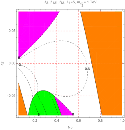
Figure 12: Contour plots of $\lambda_{2}$, $|\lambda_{12}|$ and $f_{12}$ as functions of $s_{\delta}$ and $t_{12}$. The green, orange, magenta regions are excluded by requirements that $0<\lambda_{2}<10$, $|\lambda_{12}|<10$, and $f_{12}>0$, respectively

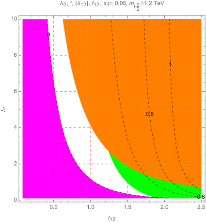
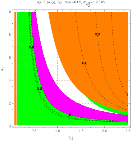
Figure 13: Contour plots of $\lambda_{2}$, $|\lambda_{12}|$ and $f_{12}$ as functions of $\lambda_{1}$ and $t_{12}$ with some fixed $m_{h^{0}_{2}}$ . The green, orange, magenta regions are excluded by requirements that $0<\lambda_{2}<10$, $|\lambda_{12}|<10$, and $f_{12}>0$, respectively

References

- (1) H. Okada, N. Okada, Y. Orikasa and K. Yagyu, Phys. Rev. D 94 (2016), 015002 [arXiv:1604.01948 [hep-ph]].
- (2) M. Aaboud et al. [ATLAS Collaboration], Phys. Lett. B 786 (2018) 114 [arXiv:1805.10197 [hep-ex]].
- (3) A. M. Sirunyan et al. [CMS Collaboration], JHEP 1811 (2018) 185 [arXiv:1804.02716 [hep-ex]].
- (4) M. Aaboud et al. [ATLAS Collaboration], Phys. Rev. D 98 (2018) 052005 [arXiv:1802.04146 [hep-ex]].
- (5) S. Heinemeyer et al. [LHC Higgs Cross Section Working Group], doi:10.5170/CERN-2013-004 arXiv:1307.1347 [hep-ph].
- (6) D. de Florian et al. [LHC Higgs Cross Section Working Group], arXiv:1610.07922 [hep-ph].
- (7) M. Aaboud et al. [ATLAS Collaboration], JHEP 1710 (2017) 112 [arXiv:1708.00212 [hep-ex]].
- (8) A. M. Sirunyan et al. [CMS Collaboration], JHEP 1811 (2018) 152 [arXiv:1806.05996 [hep-ex]].
- (9) M. Cepeda et al. [Physics of the HL-LHC Working Group], “Higgs Physics at the HL-LHC and HE-LHC,” arXiv:1902.00134 [hep-ph].
- (10) D. Fontes, J. C. Romão and J. P. Silva, JHEP 1412 (2014) 043 [arXiv:1408.2534 [hep-ph]].
- (11) S. Kanemura, M. Kikuchi, K. Mawatari, K. Sakurai and K. Yagyu, Phys. Lett. B 783 (2018) 140 [arXiv:1803.01456 [hep-ph]].
- (12) G. Bhattacharyya, D. Das, P. B. Pal and M. N. Rebelo, JHEP 1310 (2013) 081 [arXiv:1308.4297 [hep-ph]].
- (13) G. Bhattacharyya and D. Das, Phys. Rev. D 91 (2015) 015005 [arXiv:1408.6133 [hep-ph]].
- (14) T. Bandyopadhyay, D. Das, R. Pasechnik and J. Rathsman, Phys. Rev. D 99 (2019) no.11, 115021 [arXiv:1902.03834 [hep-ph]].
- (15) R. Martinez, M. A. Perez and J. J. Toscano, Phys. Lett. B 234 (1990) 503.
- (16) A. Maiezza, M. Nemevšek and F. Nesti, Phys. Rev. D 94 (2016) no.3, 035008 [arXiv:1603.00360 [hep-ph]].
- (17) C. H. Chen and T. Nomura, “Radiatively scotogenic type-II seesaw and a relevant phenomenological analysis,” arXiv:1906.10516 [hep-ph].
- (18) S. Blunier, G. Cottin, M. A. Díaz and B. Koch, Phys. Rev. D 95 (2017) no.7, 075038 [arXiv:1611.07896 [hep-ph]].
- (19) S. Kanemura, K. Mawatari and K. Sakurai, Phys. Rev. D 99 (2019) no.3, 035023 [arXiv:1808.10268 [hep-ph]].
- (20) M. Singer, J. W. F. Valle and J. Schechter, Phys. Rev. D 22 (1980) 738.
- (21) J. W. F. Valle and M. Singer, Phys. Rev. D 28 (1983) 540.
- (22) F. Pisano and V. Pleitez, Phys. Rev. D 46 (1992) 410 [hep-ph/9206242].
- (23) R. Foot, O. F. Hernandez, F. Pisano and V. Pleitez, Phys. Rev. D 47 (1993) 4158 [hep-ph/9207264].
- (24) P. H. Frampton, Phys. Rev. Lett. 69 (1992) 2889.
- (25) R. Foot, H. N. Long and T. A. Tran, Phys. Rev. D 50 (1994) no.1, R34 [hep-ph/9402243].
- (26) C. A. de Sousa Pires and O. P. Ravinez, Phys. Rev. D 58 (1998) 035008 [Phys. Rev. D 58 (1998) 35008] [hep-ph/9803409].
- (27) J. C. Montero, V. Pleitez and O. Ravinez, Phys. Rev. D 60 (1999) 076003 [hep-ph/9811280].
- (28) J. C. Montero, C. C. Nishi, V. Pleitez, O. Ravinez and M. C. Rodriguez, Phys. Rev. D 73 (2006) 016003 [hep-ph/0511100].
- (29) P. B. Pal, Phys. Rev. D 52 (1995) 1659 [hep-ph/9411406].
- (30) A. G. Dias, V. Pleitez and M. D. Tonasse, Phys. Rev. D 67 (2003) 095008 [hep-ph/0211107].
- (31) A. G. Dias and V. Pleitez, Phys. Rev. D 69 (2004) 077702 [hep-ph/0308037].
- (32) A. G. Dias, C. A. de S. Pires and P. S. Rodrigues da Silva, Phys. Rev. D 68 (2003) 115009 [hep-ph/0309058].
- (33) L. T. Hue and L. D. Ninh, Mod. Phys. Lett. A 31 (2016) no.10, 1650062 [arXiv:1510.00302 [hep-ph]].
- (34) E. Ramirez Barreto and D. Romero Abad, “Heavy long-lived fractionally charged leptons in novel model,” arXiv:1907.02613 [hep-ph].
- (35) A. J. Buras and F. De Fazio, JHEP 1608 (2016) 115 [arXiv:1604.02344 [hep-ph]].
- (36) Q. H. Cao and D. M. Zhang, “Collider Phenomenology of the 3-3-1 Model,” arXiv:1611.09337 [hep-ph].
- (37) C. X. Yue, Q. Y. Shi and T. Hua, Nucl. Phys. B 876 (2013) 747 [arXiv:1307.5572 [hep-ph]]; W. Caetano, C. A. de S. Pires, P. S. Rodrigues da Silva, D. Cogollo and F. S. Queiroz, Eur. Phys. J. C 73 (2013) no.10, 2607 [arXiv:1305.7246 [hep-ph]].
- (38) L. T. Hue, L. D. Ninh, T. T. Thuc and N. T. T. Dat, Eur. Phys. J. C 78 (2018) no.2, 128 [arXiv:1708.09723 [hep-ph]].
- (39) A. E. Carcamo Hernandez, R. Martinez and F. Ochoa, Phys. Rev. D 73 (2006) 035007 [hep-ph/0510421].
- (40) A. J. Buras, F. De Fazio and J. Girrbach, JHEP 1402 (2014) 112 [arXiv:1311.6729 [hep-ph]].
- (41) R. Martinez and F. Ochoa, Phys. Rev. D 90 (2014) no.1, 015028 [arXiv:1405.4566 [hep-ph]].
- (42) H. N. Long, N. V. Hop, L. T. Hue and N. T. T. Van, Nucl. Phys. B 943 (2019) 114629 [arXiv:1812.08669 [hep-ph]].
- (43) A. J. Buras, F. De Fazio and J. Girrbach-Noe, JHEP 1408 (2014) 039 [arXiv:1405.3850 [hep-ph]].
- (44) A. J. Buras, F. De Fazio, J. Girrbach and M. V. Carlucci, JHEP 1302 (2013) 023 [arXiv:1211.1237 [hep-ph]].
- (45) W. Caetano, C. A. de S. Pires, P. S. Rodrigues da Silva, D. Cogollo and F. S. Queiroz, Eur. Phys. J. C 73 (2013) no.10, 2607 [arXiv:1305.7246 [hep-ph]].
- (46) A. E. Cárcamo Hernández, Y. H. Velásquez and N. A. Pérez-Julve, “A 3-3-1 model with low scale seesaw mechanisms,” arXiv:1905.02323 [hep-ph].
- (47) C. Degrande, K. Hartling and H. E. Logan, Phys. Rev. D 96 (2017) no.7, 075013 Erratum: [Phys. Rev. D 98 (2018) no.1, 019901] [arXiv:1708.08753 [hep-ph]].
- (48) L. T. Hue, A. B. Arbuzov, T. T. Hong, T. P. Nguyen, D. T. Si and H. N. Long, Eur. Phys. J. C 78 (2018) no.11, 885 [arXiv:1712.05234 [hep-ph]].
- (49) U. Haisch and G. Polesello, JHEP 1809 (2018) 151 doi:10.1007/JHEP09(2018)151 [arXiv:1807.07734 [hep-ph]].
- (50) S. Descotes-Genon, M. Moscati and G. Ricciardi, Phys. Rev. D 98 (2018) no.11, 115030 [arXiv:1711.03101 [hep-ph]].
- (51) L. T. Hue and L. D. Ninh, Eur. Phys. J. C 79 (2019) no.3, 221 [arXiv:1812.07225 [hep-ph]].
- (52) N. Craig and S. Thomas, JHEP 1211 (2012) 083 [arXiv:1207.4835 [hep-ph]].
- (53) A. J. Buras, F. De Fazio, J. Girrbach, and M. V. Carlucci, JHEP 02, 023 (2013), arXiv:1211.1237.
- (54) B. L. Sánchez-Vega, G. Gambini and C. E. Alvarez-Salazar, Eur. Phys. J. C 79 (2019) no.4, 299 [arXiv:1811.00585 [hep-ph]].
- (55) K. Huitu and N. Koivunen, “Suppression of scalar mediated FCNCs in a -model,” arXiv:1905.05278 [hep-ph].
- (56) R. A. Diaz, R. Martinez and F. Ochoa, Phys. Rev. D 72, 035018 (2005) [hep-ph/0411263].
- (57) J. F. Gunion, H. E. Haber, G. L. Kane and S. Dawson, “The Higgs Hunter’s Guide,” Front. Phys. 80 (2000) 1.
- (58) M. Tanabashi et al. [Particle Data Group], Phys. Rev. D 98 (2018) no.3, 030001.
- (59) G. Aad et al. [ATLAS and CMS Collaborations], JHEP 1608 (2016) 045 [arXiv:1606.02266 [hep-ex]].
- (60) S. Banerjee and N. Chakrabarty, JHEP 1905 (2019) 150 [arXiv:1612.01973 [hep-ph]].
- (61) S. De Lope Amigo, W. M. Y. Cheung, Z. Huang and S. P. Ng, JCAP 0906 (2009) 005 [arXiv:0812.4016 [hep-ph]].
- (62) B. Eiteneuer, A. Goudelis and J. Heisig, Eur. Phys. J. C 77 (2017) no.9, 624 [arXiv:1705.01458 [hep-ph]].
- (63) A. Belyaev, G. Cacciapaglia, I. P. Ivanov, F. Rojas-Abatte and M. Thomas, Phys. Rev. D 97 (2018) no.3, 035011 [arXiv:1612.00511 [hep-ph]].
- (64) S. Filippi, W. A. Ponce and L. A. Sanchez, Europhys. Lett. 73 (2006) 142 [hep-ph/0509173].
- (65) D. Cogollo, A. X. Gonzalez-Morales, F. S. Queiroz and P. R. Teles, JCAP 1411 (2014) no.11, 002 [arXiv:1402.3271 [hep-ph]].
- (66) C. A. de S.Pires and P. S. Rodrigues da Silva, JCAP 0712 (2007) 012 [arXiv:0710.2104 [hep-ph]].
- (67) S. M. Boucenna, A. Celis, J. Fuentes-Martin, A. Vicente and J. Virto, JHEP 1612 (2016) 059 [arXiv:1608.01349 [hep-ph]].
- (68) M. Spira, Fortsch. Phys. 46 (1998) 203 [hep-ph/9705337].
- (69) Y. A. Coutinho, V. Salustino Guimarães and A. A. Nepomuceno, Phys. Rev. D 87 (2013) no.11, 115014 [arXiv:1304.7907 [hep-ph]].
- (70) M. M. Ferreira, T. B. de Melo, S. Kovalenko, P. R. D. Pinheiro and F. S. Queiroz, “Lepton Flavor Violation and Collider Searches in a Type I + II Seesaw Model,” arXiv:1903.07634 [hep-ph].
- (71) H. N. Long, N. V. Hop, L. T. Hue, N. H. Thao and A. E. Carcamo Hernandez, Phys. Rev. D 100, No 1, 015004 (2019) [arXiv:1810.00605 [hep-ph]].
- (72) M. Aaboud et al. [ATLAS Collaboration], JHEP 1801 (2018) 055 [arXiv:1709.07242 [hep-ex]].
- (73) A. M. Sirunyan et al. [CMS Collaboration], JHEP 1806 (2018) 120 [arXiv:1803.06292 [hep-ex]].
- (74) G. Aad et al. [ATLAS Collaboration], “Search for high-mass dilepton resonances using 139 fb-1 of collision data collected at 13 TeV with the ATLAS detector,” arXiv:1903.06248 [hep-ex].
- (75) F. F. Freitas, C. A. de S. Pires and P. Vasconcelos, Phys. Rev. D 98 (2018) no.3, 035005 [arXiv:1805.09082 [hep-ph]].
- (76) G. Arcadi, M. Lindner, J. Martins and F. S. Queiroz, “New Physics Probes: Atomic Parity Violation, Polarized Electron Scattering and Neutrino-Nucleus Coherent Scattering,” arXiv:1906.04755 [hep-ph].
- (77) G. Corcella, C. Corianò, A. Costantini and P. H. Frampton, Phys. Lett. B 785 (2018) 73 [arXiv:1806.04536 [hep-ph]].
- (78) S. Kanemura, T. Kasai and Y. Okada, Phys. Lett. B 471 (1999) 182 [hep-ph/9903289].
- (79) G. Aad et al. [ATLAS Collaboration], JHEP 1511 (2015) 206 [arXiv:1509.00672 [hep-ex]].
- (80) J. Haller, A. Hoecker, R. Kogler, K. Mönig, T. Peiffer and J. Stelzer, Eur. Phys. J. C 78 (2018) no.8, 675 [arXiv:1803.01853 [hep-ph]].
- (81) P. M. Ferreira, M. Mühlleitner, R. Santos, G. Weiglein and J. Wittbrodt, JHEP 1909 (2019) 006 [arXiv:1905.10234 [hep-ph]].
- (82) K. Kainulainen, V. Keus, L. Niemi, K. Rummukainen, T. V. I. Tenkanen and V. Vaskonen, JHEP 1906 (2019) 075 [arXiv:1904.01329 [hep-ph]].
- (83) K. S. Babu and S. Jana, JHEP 1902 (2019) 193 [arXiv:1812.11943 [hep-ph]].
- (84) M. Aaboud et al. [ATLAS Collaboration], Eur. Phys. J. C 78 (2018) no.1, 24 [arXiv:1710.01123 [hep-ex]].
- (85) A. G. Dias and V. Pleitez, Phys. Rev. D 80 (2009) 056007 [arXiv:0908.2472 [hep-ph]].
- (86) G. Passarino and M. J. G. Veltman, Nucl. Phys. B 160 (1979) 151.
- (87) T. Hahn and M. Perez-Victoria, Comput. Phys. Commun. 118 (1999) 153 [hep-ph/9807565].
- (88) A. Palcu, “On trilinear terms in the scalar potential of 3-3-1 gauge models,” arXiv:1907.00572 [hep-ph].
- (89) V. Khachatryan et al. [CMS Collaboration], Eur. Phys. J. C 74 (2014) no.10, 3076 [arXiv:1407.0558 [hep-ex]].
- (90) G. Aad et al. [ATLAS Collaboration], Phys. Rev. D 90 (2014) no.11, 112015 [arXiv:1408.7084 [hep-ex]].
- (91) L. T. Hue, A. B. Arbuzov, N. T. K. Ngan and H. N. Long, Eur. Phys. J. C 77 (2017) no.5, 346 [arXiv:1611.06801 [hep-ph]].
- (92) X. G. He and G. Valencia, Phys. Lett. B 779 (2018) 52 [arXiv:1711.09525 [hep-ph]].
- (93) M. Abdullah, J. Calle, B. Dutta, A. Flórez and D. Restrepo, Phys. Rev. D 98 (2018) no.5, 055016 [arXiv:1805.01869 [hep-ph]].
- (94) C. X. Yue and S. S. Jia, J. Phys. G 46 (2019) no.7, 075001.