Position measurement-induced collapse states:
Proposal of an experiment

Abstract

The quantum mechanical treatment of diffraction of particles, based on the standard postulates of quantum mechanics and the postulate of existence of quantum trajectories, leads to the ‘position measurement-induced collapse’ (PMIC) states. An experimental set-up to test these PMIC states is proposed. The apparatus consists of a modified Lloyd’s mirror in optics, with two reflectors instead of one. The diffraction patterns for this case predicted by the PMIC formalism are presented. They exhibit quantum fractal structures in space-time called ‘quantum carpets’, first discovered by Berry (1996). The PMIC formalism in this case closely follows the ‘boundary bound diffraction’ analysed in a previous work by Tounli, Alverado and Sanz (2019). In addition to obtaining their results, we have shown that the time evolution of these collapsed states also leads to Fresnel and Fraunhofer diffractions. It is anticipated that the verification of PMIC states by this experiment will help to better understand collapse of the wave function during quantum measurements.


Keywords $\ \ \diamond$ Single slit diffraction $\ \ \diamond$ matter waves $\ \ \diamond$ Quantum measurement $\ \ \diamond$ Wave function collapse$\ \ \diamond$ Quantum formalism

1 Introduction

With the advancement of technology in dealing with single-particle systems, quantum theory has now entered a new phase, namely that of ‘quantum measurement’ [1, 2]. This has led to new operational interpretations of quantum mechanics. In classical mechanics of a system of particles, measurement of position is of prime concern. The case of quantum mechanics is not very different either. Heisenberg’s thought experiment, in which the position of a particle is measured with an idealised ‘gamma ray microscope’, has been central to its understanding. However, quantum theory lacked a proper operational definition of ‘position measurement’ for a long time. Lamb [3] has made an attempt in this direction, observing that the above thought experiment by Heisenberg can only be considered as a scattering experiment. Recently operational approaches to quantum position measurement have gained renewed attention.

The question whether single-slit diffraction can be treated as quantum measurement of position of a particle was raised by Marcella [4] and was followed up in [5, 6]. In a recent paper, we have obtained a satisfactory, affirmative answer [7] to the above question using the standard axioms of quantum mechanics, together with nonlocal quantum trajectory representations. As in [4], we have considered a particle that passes through a slit at a time $t=t_{M}$ and assumed that its wave function collapses to a rectangular function. We then expressed this collapsed rectangular wave function (which can be considered as a superposition of position eigenfunctions) in terms of the energy eigenfunctions in the relevant case. Lastly, unitary time-evolution of the state for $t\geq t_{M}$ is introduced and this results in what we called the position measurement-induced collapse (PMIC) state. The formalism could lead to a unified quantum description of Fresnel (near-field) and Fraunhofer (far-field) diffractions. The result that a single quantum expression describes both kind of diffractions was claimed to be the first its kind.

In the present Letter we describe the PMIC states for a particle whose position is measured when it is in an infinite potential well and then suggest an experimental set-up where this formalism can be tested. For this purpose, a modified single-slit diffraction arrangement, which can be considered as a double Lloyd’s mirror apparatus, is proposed. Here we have adopted a purely quantum mechanical approach based on PMIC states that can be verified with experiment.

The present work has some closely related antecedents in [8] and [9]. In the former, Berry has computed the probability density corresponding to a wave function of a particle in a box that evolves from an initial one with a discontinuity at its walls. This work has drawn attention to some unexpected fractal properties of this function. In a recent paper, Tounli, Alvarado and Sanz [9] have considered ‘boundary-bound diffraction’ of a spatially localised matter wave with discontinuity at its boundary. Thereafter, the matter wave is considered to evolve freely beyond the initial localisation region, but is frustrated by the presence of hard-wall-type boundaries of a cavity that contains it. Both these works lead to fractal functions in space and time. In the latter paper, the authors have noted that the development of space-time pattern inside the cavity depends on (1) the shape of the wave function $f(x)$ in the initial localisation region, (2) the mass of the particle considered and (3) the relative extension of the initial state with respect to the total length spanned by the cavity. However, they did not identify any Fresnel or Fraunhofer patterns in their analysis. Instead, they state that because of the presence of confining boundaries, even in the cases of an increasingly large box length, no Fraunhofer-like diffraction features can ever be observed at any time. We have reproduced the fractal patterns obtained by them, which are referred to as ‘quantum carpets’ for the cases mentioned. The revival of wave functions, as found in these papers are also observed. In addition, we have computed the probability density of particles on the screen placed at various distances from the slit. Contrary to their conclusion regarding diffraction patterns, we found that Fresnel and Fraunhofer patterns are indeed present in them. The diffraction experiment suggested by us shall help to demonstrate the above fractal and nonfractal features of the wave function at various times and also the predicted revival distances to the screen.

This paper is organised as follows. The theoretical formulation of PMIC states is presented in Sec. 2. The prediction of the probability patterns that may be obtained for the case of a particle in an infinite potential well for various times is made in Sec. 3. In Sec. 4, the experimental arrangement that can produce these patterns is described. The last section comprises a discussion.

2 PMIC states

In this section, a general formulation of the PMIC states that closely follows the discussion in [8, 9] is made. Since our interest is to apply this to an actual experiment of diffraction of matter waves, we continue to view it as position measurement-induced collapse state, defined using the postulate of reduction of the wave function in quantum mechanics [10]. According to this postulate, if a measurement of an observable ${\cal A}$ on a system in the state $\ket{{\psi}}$ has yielded the result $\alpha_{0}$ to within an accuracy $\Delta\alpha$, the state of the system immediately after the measurement is described by

$$\ket{\psi^{\alpha_{0},\Delta\alpha}}=\frac{1}{\sqrt{\bra{{\psi}}P_{\Delta\alpha}(\alpha_{0})\ket{{\psi}}}}P_{\Delta\alpha}(\alpha_{0})\ket{{\psi}},$$ (1)

with the projection operator

$$P_{\Delta\alpha}(\alpha_{0})=\int_{\alpha_{0}-\Delta\alpha/2}^{\alpha_{0}+\Delta\alpha/2}d\alpha\ket{{\alpha}}\bra{{\alpha}}.$$ (2)

Here $\{\ket{{\alpha}}\}$ is the set of eigenstates of ${\cal A}$ that serves as a complete orthonormal basis. Let us consider the collapse of the wave function of a particle in one-dimension with coordinate $y$, under the measurement ${\cal A}$. With $\braket{{\alpha}}{{\psi}}\equiv{c}(\alpha)$ and $\braket{y}{{\alpha}}\equiv v({\alpha},y)$, one can write the collapsed wave function $\ket{\psi^{\alpha_{0},\Delta\alpha}}$ in the position representation as

$$\psi_{y}^{\alpha_{0},\Delta\alpha}(y)=\frac{1}{\sqrt{\int_{\alpha_{0}-\Delta\alpha/2}^{\alpha_{0}+\Delta\alpha/2}d\alpha\mid{c}(\alpha)\mid^{2}}}\int_{\alpha_{0}-\Delta\alpha/2}^{\alpha_{0}+\Delta\alpha/2}d\alpha\;{c}(\alpha)\;v({\alpha},y).$$ (3)

Now consider the case where ${\cal A}$ is the position operator for the particle, representing position measurement. Let us denote the eigenvalues and eigenvectors in this case as $y^{\prime}$ and $\ket{y^{\prime}}$, respectively. Also let the measurement of position give the value of $y$ in the interval $[y_{0}-a/2,y_{0}+a/2]$; i.e., with an accuracy $\Delta y\equiv a$. Then the above equation can be rewritten with $\alpha=y^{\prime}$, $\alpha_{0}=y_{0}$ and $\Delta\alpha=a$. We also have ${c}(y^{\prime})\equiv\braket{y^{\prime}}{{\psi}}={\psi}(y^{\prime})$ and $v({y^{\prime}},y)\equiv\braket{y}{y^{\prime}}=\delta(y-y^{\prime})$. The Dirac delta function in the latter expression is the position eigenstate in the position representation. Eq. (3) now becomes

$$\psi_{y}^{y_{0},a}(y)=\frac{1}{\sqrt{\int_{y_{0}-a/2}^{y_{0}+a/2}dy^{\prime}\mid{\psi}(y^{\prime})\mid^{2}}}\int_{y_{0}-a/2}^{y_{0}+a/2}dy^{\prime}\;{\psi}(y^{\prime})\;\delta(y-y^{\prime}).$$ (4)

In [7], the PMIC states is defined using this expression for collapsed states. First assume that immediately after the above collapse, the particle is in a potential $V$, where the eigenstates of energy are $\ket{u_{n}}$ and the corresponding position space energy eigenfunctions are $u_{n}(y)\equiv\braket{y}{u_{n}}$. We can use the closure representation of Dirac delta function [16]

$$\sum_{n=0}^{\infty}u_{n}^{\star}(y^{\prime})u_{n}(y)=\delta(y-y^{\prime}),$$ (5)

to represent the position eigenstate of the particle while it is detected at the point $y^{\prime}$ at $t=t_{M}$. This helps to expand the collapsed wave function (4) as an infinite series, given by

$$\psi_{y}^{y_{0},a}(y)=\frac{1}{\sqrt{\int_{y_{0}-a/2}^{y_{0}+a/2}dy^{\prime}\mid{\psi}(y^{\prime})\mid^{2}}}\int_{y_{0}-a/2}^{y_{0}+a/2}dy^{\prime}\;{\psi}(y^{\prime})\;\sum_{n=0}^{\infty}u_{n}^{\star}(y^{\prime})u_{n}(y).$$ (6)

The base functions are chosen to be the eigenfunctions of the Hamiltonian operator to aid the introduction of unitary time-evolution of the system.

Let the above wave function be denoted as $\psi_{y}^{y_{0},a}(y)\equiv\Psi_{y}^{y_{0},a}(y,t_{M})$ where $t_{M}$ is the time at which the measurement is made. Now one can introduce the time-evolution of the wave function of the particle to obtain the PMIC states for $t\geq t_{M}$ as

$$\Psi_{y}^{y_{0},a}(y,t)=\frac{1}{\sqrt{\int_{y_{0}-a/2}^{y_{0}+a/2}dy^{\prime}\mid{\psi}(y^{\prime})\mid^{2}}}\sum_{n=0}^{N}\left[\int_{y_{0}-a/2}^{y_{0}+a/2}dy^{\prime}\psi(y^{\prime})\;u_{n}^{\star}(y^{\prime})\right]u_{n}(y)e^{-iE_{n}(t-t_{M})/\hbar},$$ (7)

where the upper limit $N\rightarrow\infty$ may be taken. Here $E_{n}$ are the energy eigenvalues of the particle when it is in this potential.

Let us now assume for simplicity that the wave function before collapse $\braket{y}{{\psi}}\equiv{\psi}(y)$ is a constant over the small interval of width $a$. Then the collapsed wave function $\braket{y}{\psi^{y_{0},a}}\equiv\psi^{y_{0},a}(y)$ in the above equation can be considered as a rectangular wave function at the instant of collapse, given by

$$\psi_{y}^{y_{0},a}(y)=\left\{\begin{array}[]{lr}\frac{1}{\sqrt{a}}&\qquad y_{0}-a/2\leq y\leq y_{0}+a/2\\ 0&\qquad\hbox{for other values of $y$.}\end{array}\right.$$ (10)

In this case, the PMIC wave function becomes

$$\Psi_{y}^{y_{0},a}(y,t)=\frac{1}{\sqrt{a}}\sum_{n=0}^{N}\left[\int_{y_{0}-a/2}^{y_{0}+a/2}dy^{\prime}\;u_{n}^{\star}(y^{\prime})\right]u_{n}(y)e^{-iE_{n}(t-t_{M})/\hbar}.$$ (11)

Now consider that the potential $V$ experienced by the particle after collapse is an infinite potential well, with $V=0$ in the interval $-L/2\leq y\leq L/2$ and $V=\infty$ outside. Let the measurement, made at time $t_{M}$, give the particle’s position as $y_{0}$ with an accuracy $a$, where $y_{0}$ is contained inside the interval $[-L/2,L/2]$. Following the discussion above, one can express the above PMIC wave function in terms of the eigenstates of energy of the particle in the potential well by choosing

$$u_{n}(y)=A\sin\left[\frac{n\pi}{L}\left(y+\frac{L}{2}\right)\right],$$ (12)

and

$$E_{n}=\frac{n^{2}\pi^{2}\hbar^{2}}{2mL^{2}}$$ (13)

in Eq. (11), with $n=1,2,3,..$. We have plotted $|\Psi_{y}^{y_{0},a}(y,t)|^{2}$ against $y$ using Eq. (11), for various fixed values of $t$, with $t_{M}=0$. We also chose $\hbar/m=1$ and $L=1$. (The fundamental period, which is called the revival time, is then $T=4/\pi$.) The results are discussed in the next section.

Such expansions as that in Eq. (10) was performed in [8, 9] to obtain surprising fractal patterns called quantum carpets. In the next section, we reproduce their results. The spread in rectangular function for $t>0$ shows several interesting features. Careful analysis also reveals that these patterns contain Fresnel and Fraunhofer diffraction patterns.

3 Prediction of patterns

The PMIC patterns described by Eq. (11) for the case given in Eq. (12) and (13) are presented here with $t_{M}=0$. First, we plot the quantum carpet in space-time for this case of rectangular wave function, with $L=50$, $m/\hbar=1$, $y_{0}=0$, $a=10$ and $N=500$. The obtained pattern, shown in Fig. 1, is very similar to the one in [9].

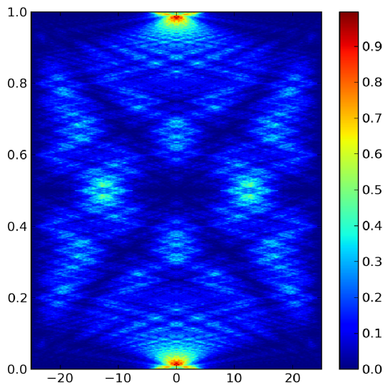
Figure 1: Quantum carpet

In an experiment, what one observes is the distribution of particles at some fixed values of $t$. We have plotted such distributions for various fixed values of $t$, and for different values of $N$, $y_{0}$ and $a$. To begin with, we chose $L=1$, $y_{0}=0.245$ and $a=0.01$. For comparison, the patterns obtained for $N=100$, $N=1000$, $N=10000$ and $N=50000$ are given in Fig. 2 (a)-(d). An almost exact (by eye) rectangular function is reproduced with $N=50,000$ and in all the remaining cases discussed below, we have taken this value of $N$ for calculations.

, , ,

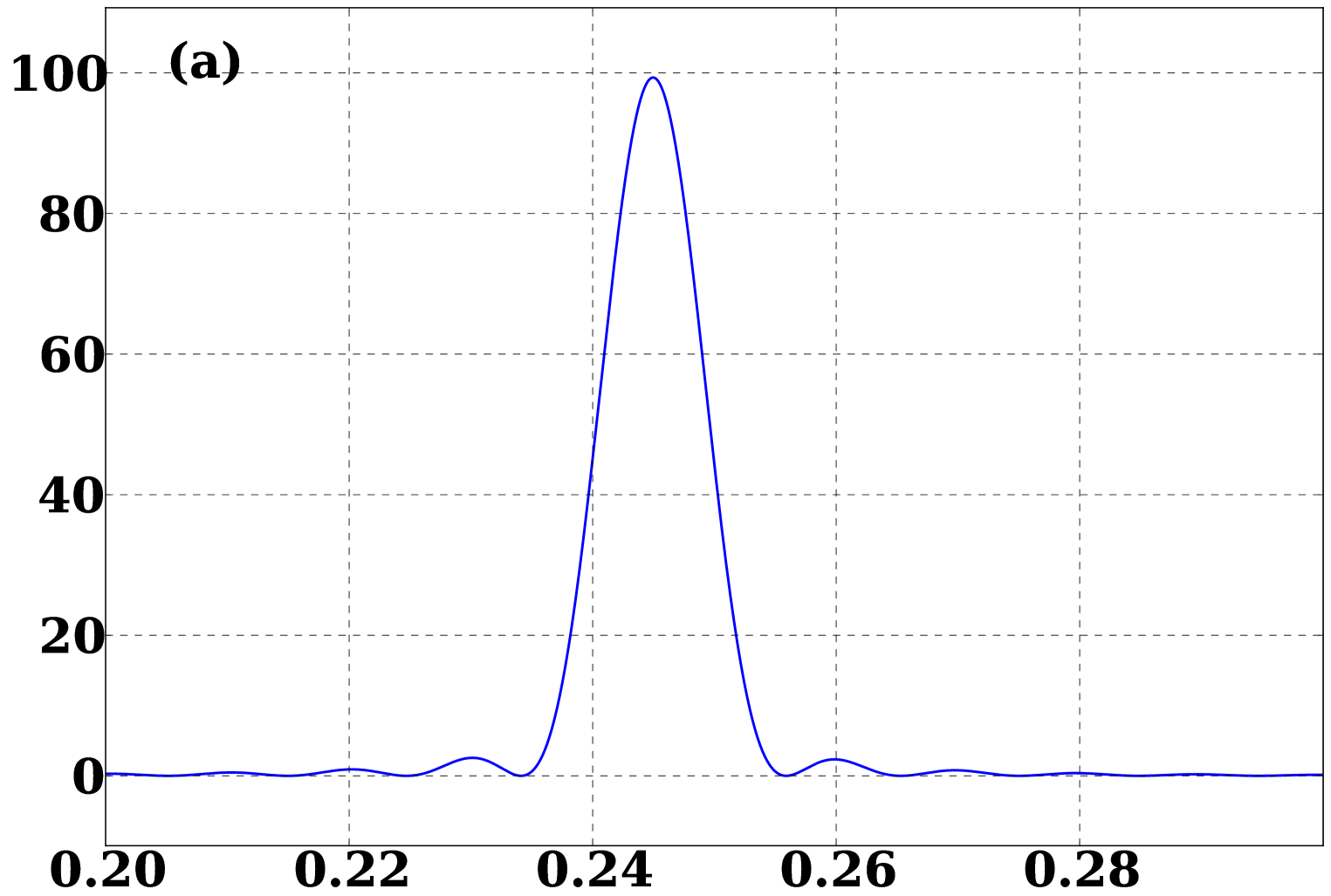
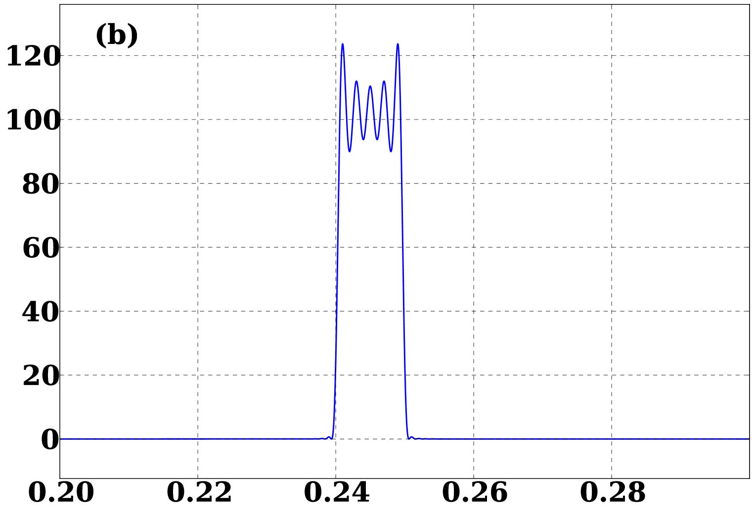
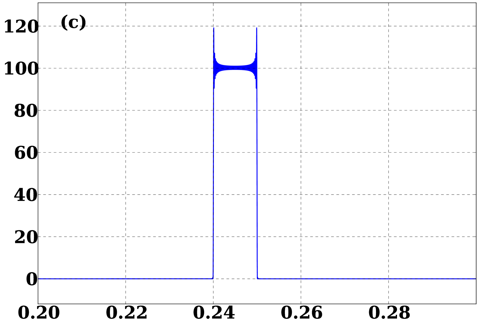
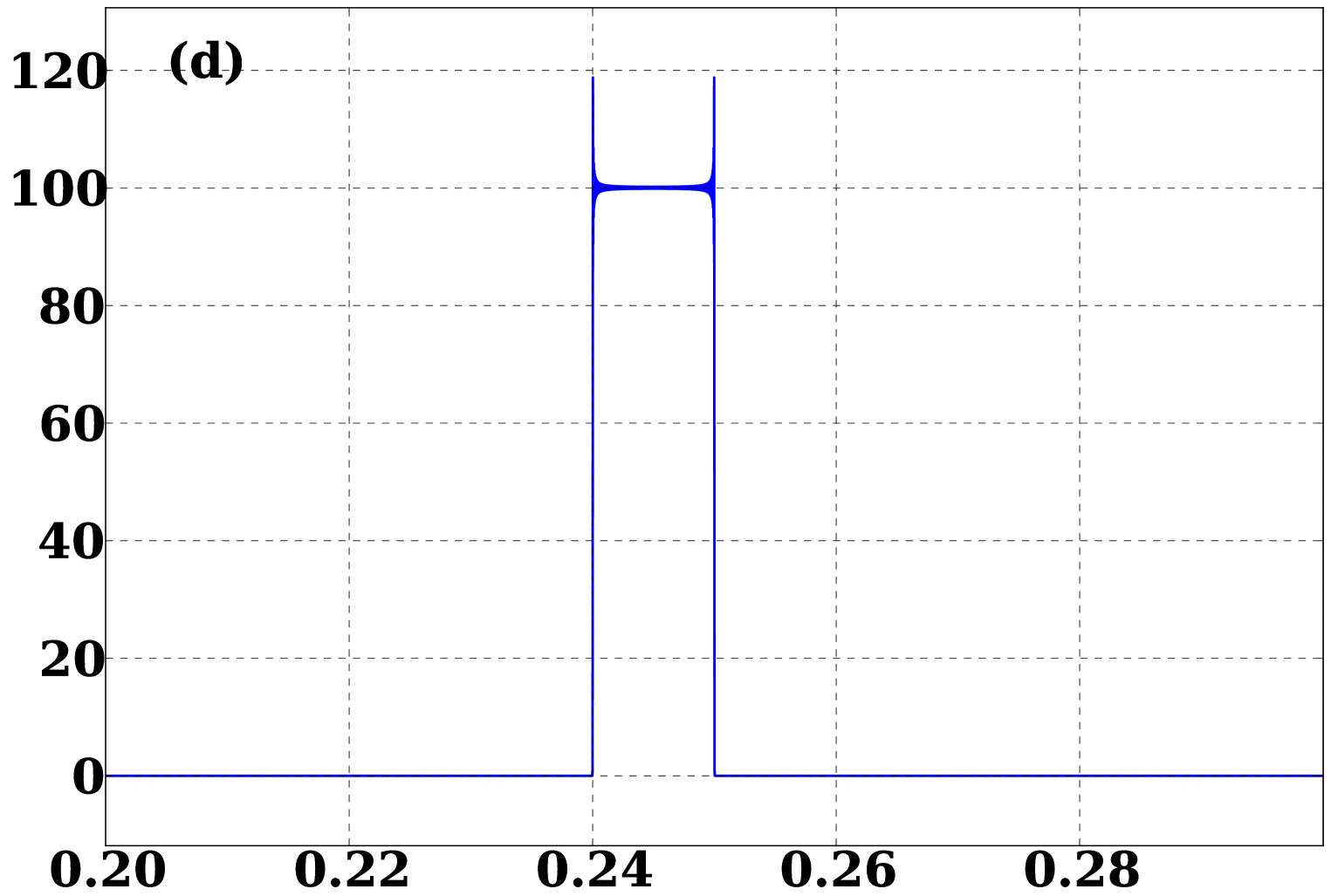
Figure 2: PMIC wave function plotted for time $t=0$, with the values of (a) $N=100$ (b) $N=1000$, (c) $N=10000$ (d) $N=50000$

Next, it may be noted that though the rectangular wave function can be obtained for $t=0$ [Fig. 3(a), same as Fig. 2(d)], a slight variation in $t$ changes this to a Fresnel-type pattern. Here we show such a pattern obtained at $t=2\times 10^{-5}$ units in Fig. 3 (b). Further, at a time $t=4\times 10^{-5}$ units, it appears almost similar to that of Fraunhofer diffraction, as shown in Fig. 3 (c).

, ,

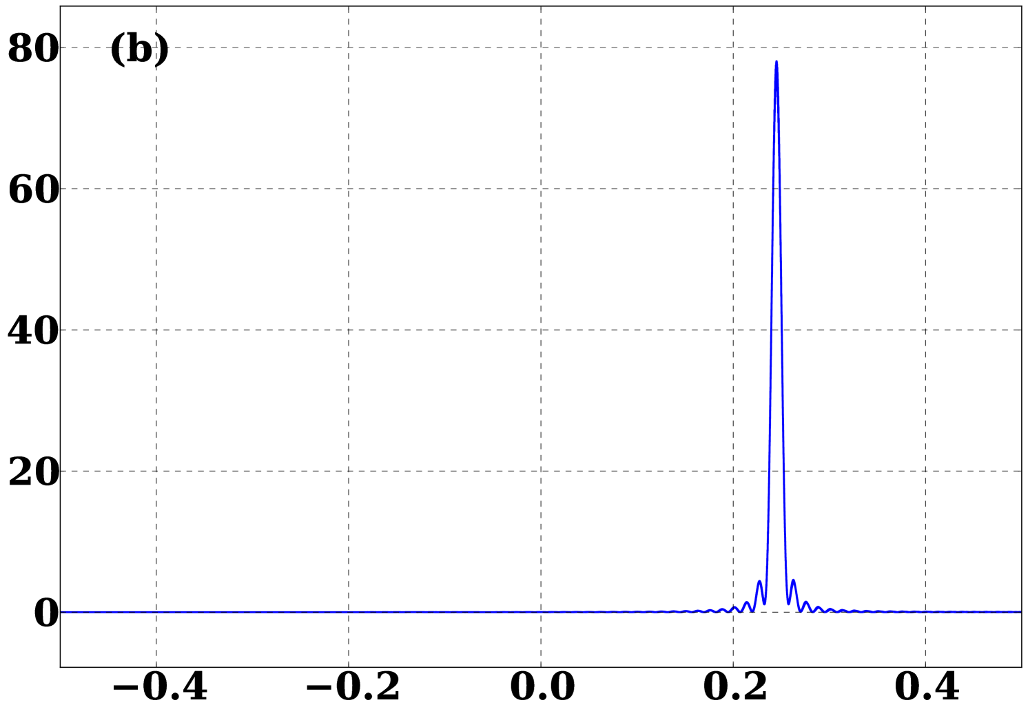
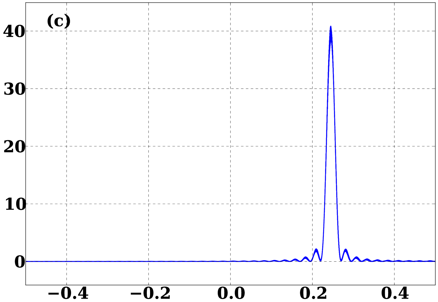
Figure 3: PMIC wave function plotted for time $N=50000$, with the values of (a) $t=0$ (b) $t=2\times 10^{-5}$, (c) $t=4\times 10^{-5}$

When $t$ is increased further, other interesting patterns appear. Varying time in steps of $10^{-4}$ units gives the patterns in Fig. 4, which show that the wave function and hence the probability pattern begin to spread.

,

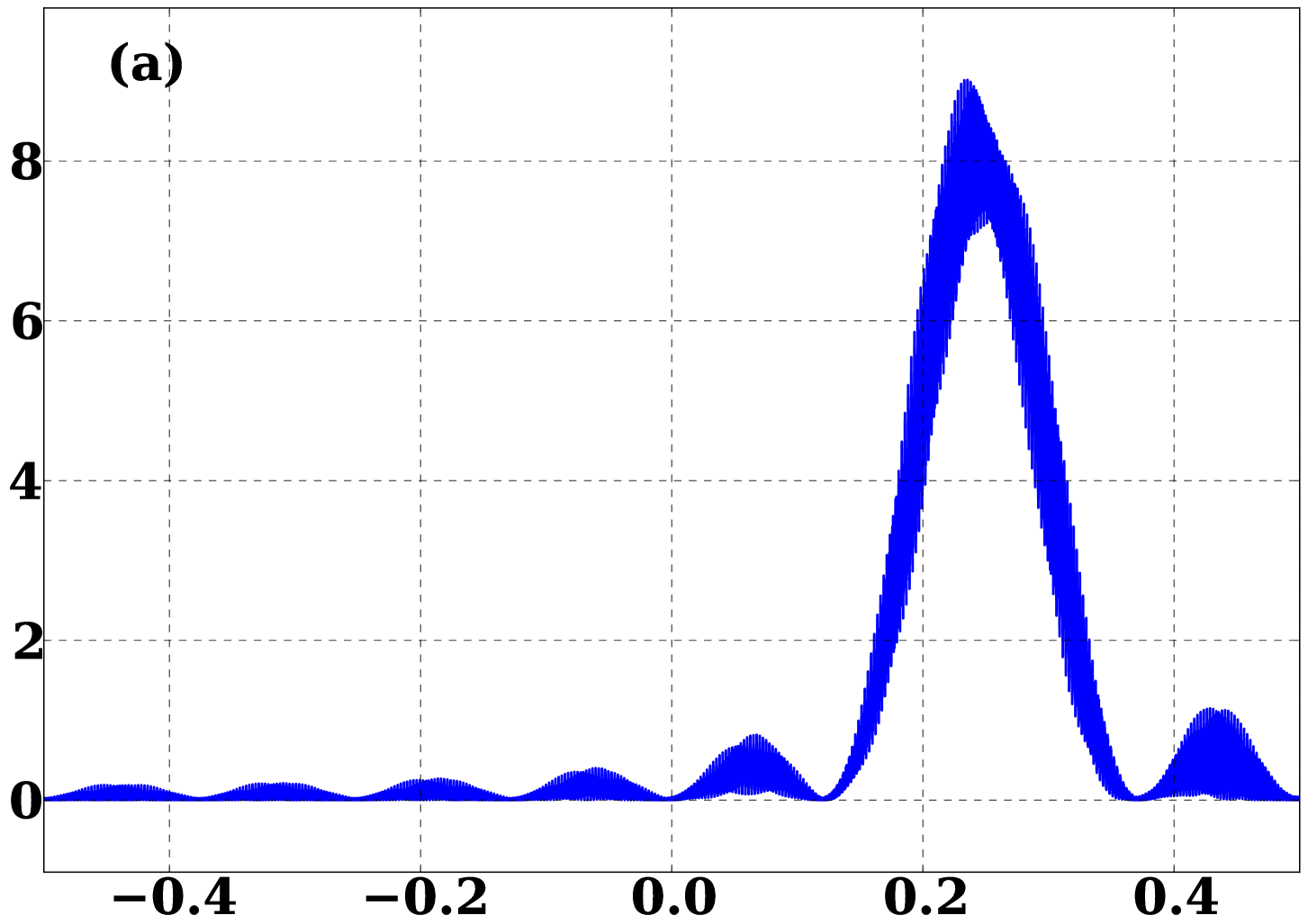
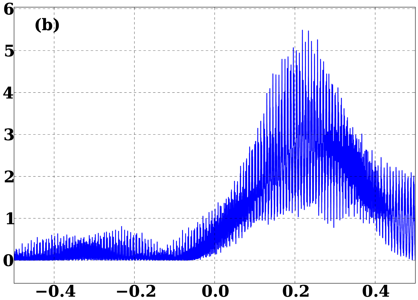
Figure 4: PMIC wave function plotted for time $N=50000$, with the values of (a) $t=2\times 10^{-4}$ (b) $t=6\times 10^{-4}$

It may be noted that in all the above cases, the values of time are irrational submultiples of $T=4/\pi$. As observed in [8, 9], the patterns in such cases have fractal structure. This can be seen for cases with still larger values of time. The following figures in Fig. (5) (a)-(d) show the respective patterns, for values of $t=2\times 10^{-3}$, $t=4\times 10^{-3}$, $t=6\times 10^{-3}$ and $t=8\times 10^{-3}$.

, , ,

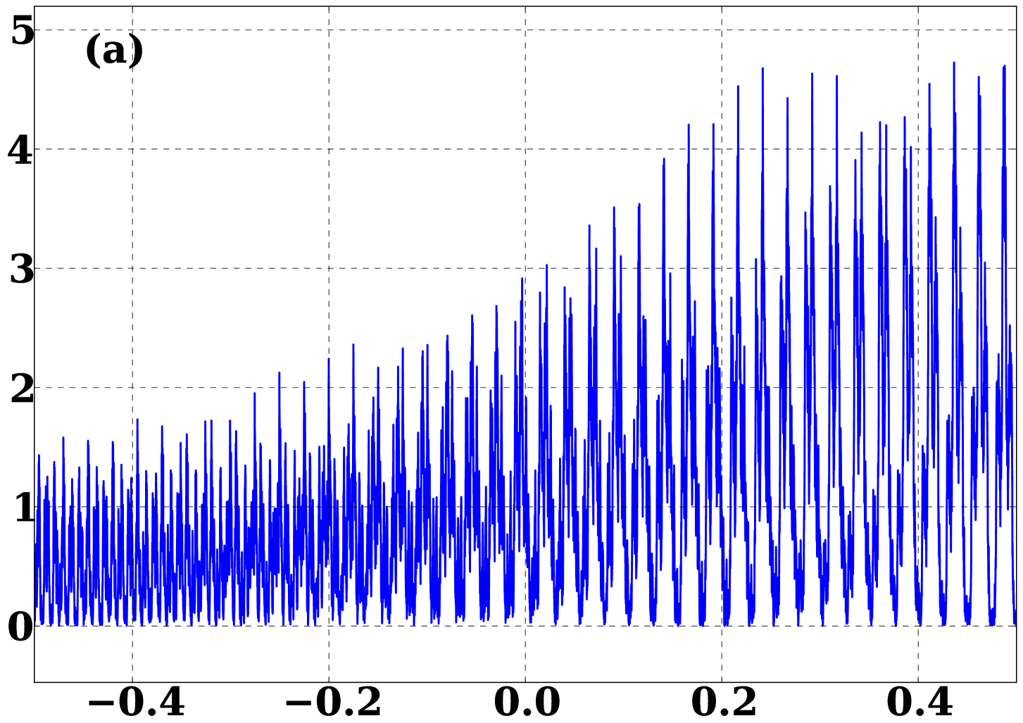
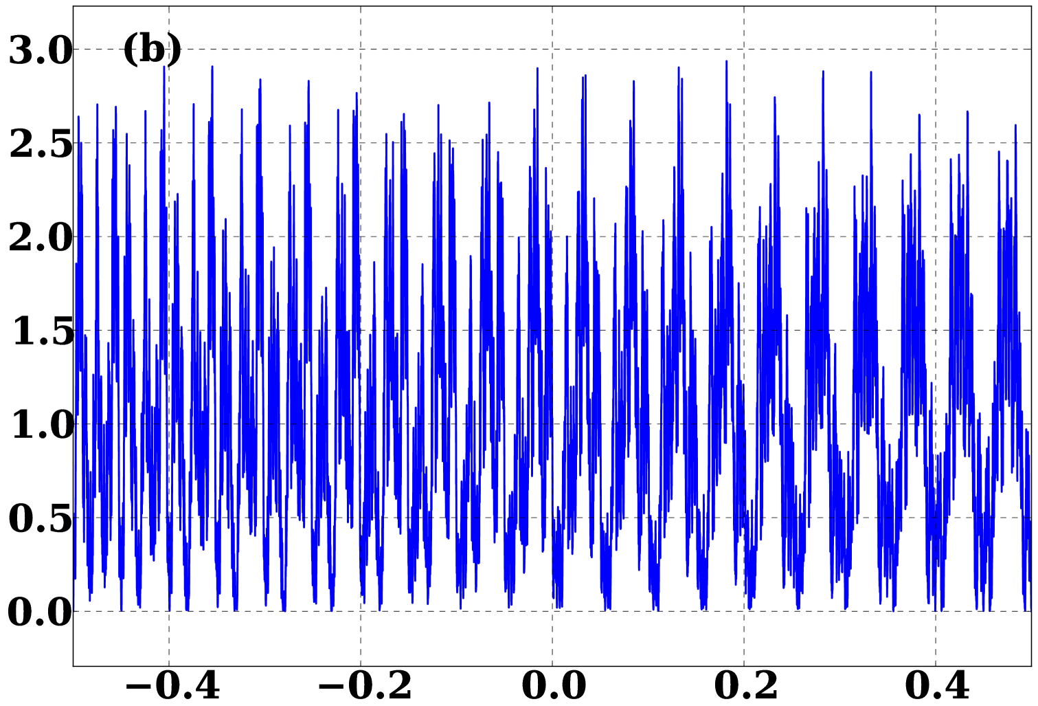
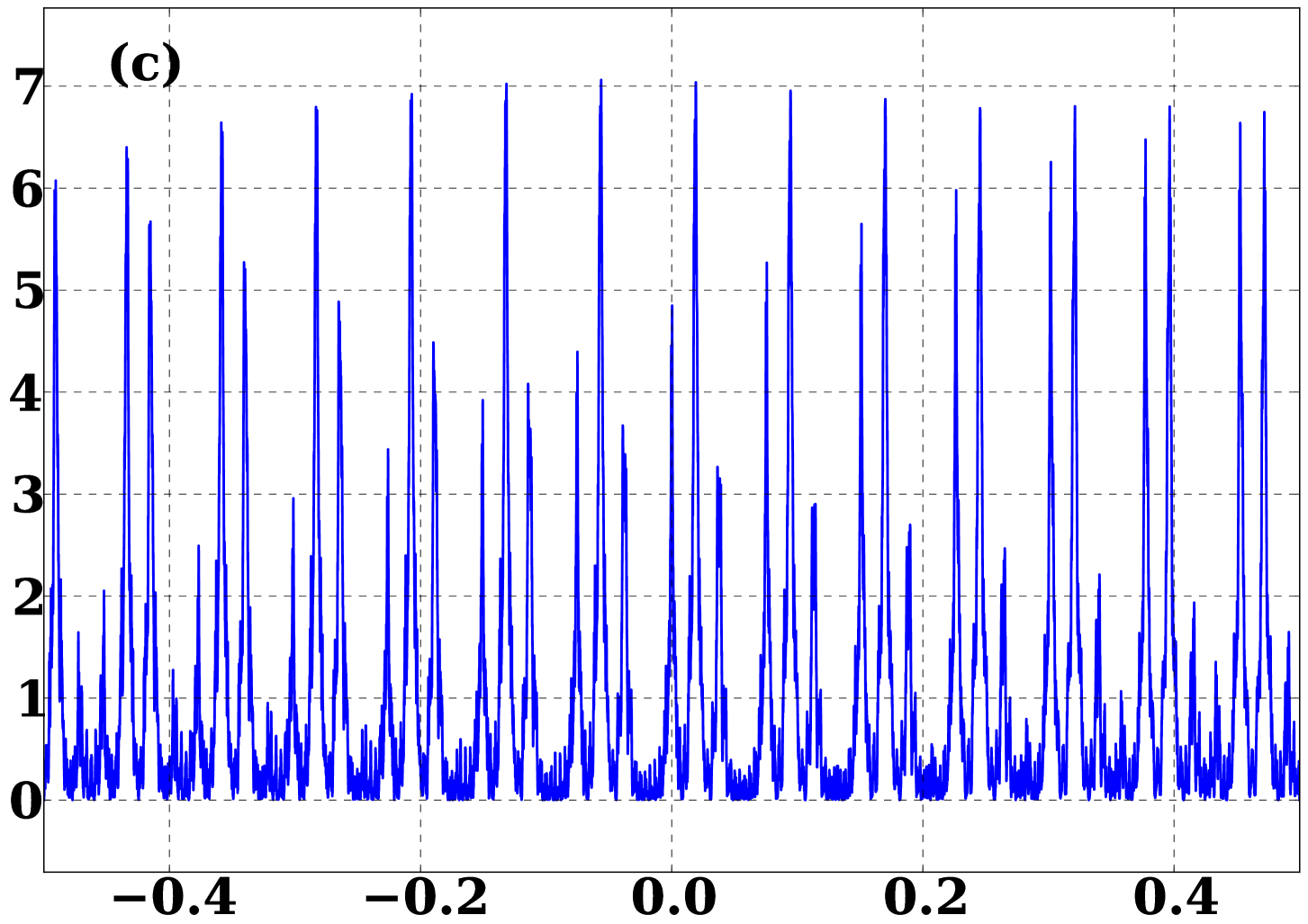
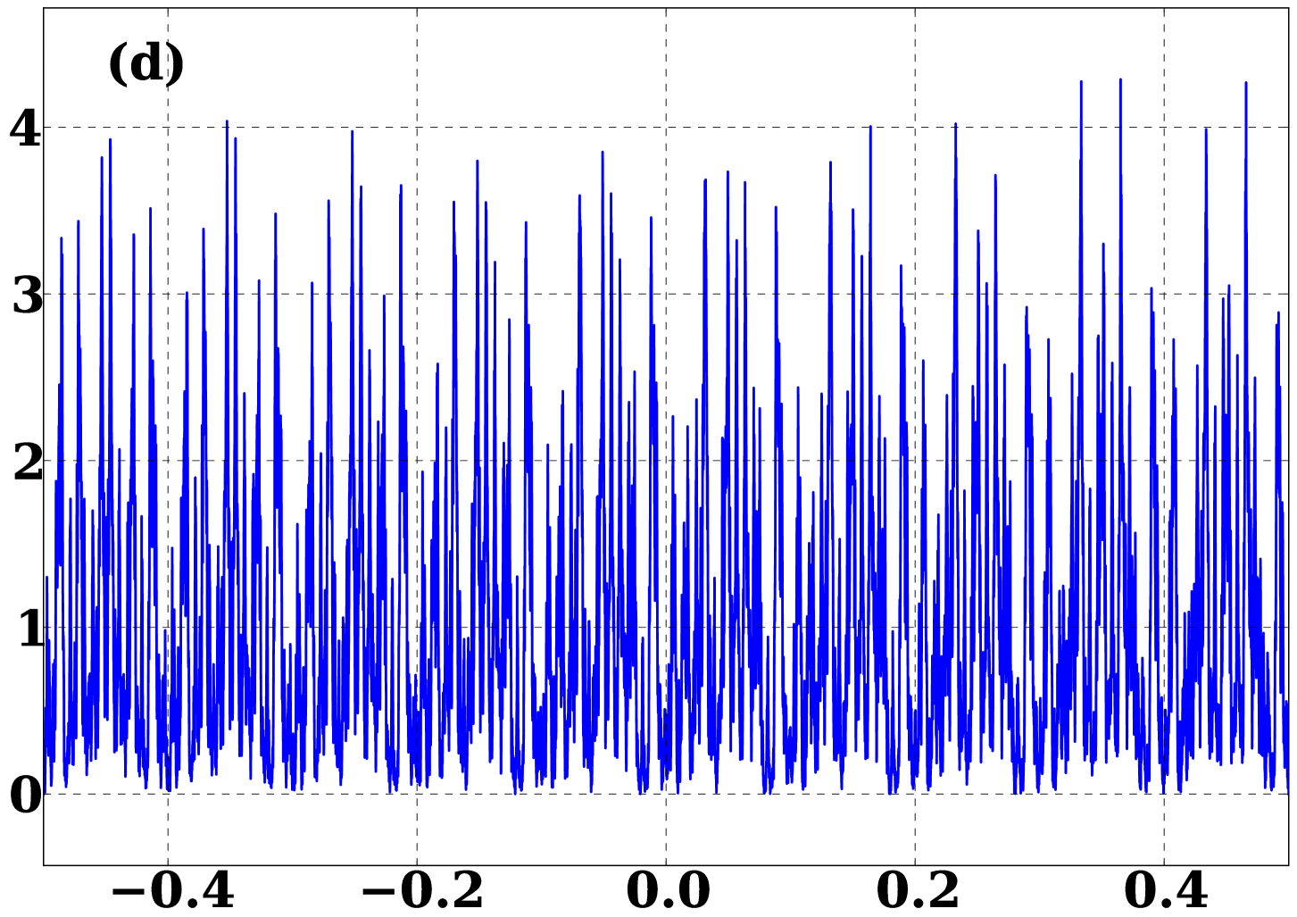
Figure 5: PMIC wave function plotted for time $N=50000$, with the values of (a) $t=2\times 10^{-3}$ (b) $t=4\times 10^{-3}$, (c) $t=6\times 10^{-3}$ and $t=8\times 10^{-3}$

Next consider cases where time $t$ is some rational submultiple of the revival time $T=4/\pi$. Not surprisingly, at half this time-period; i.e., at the time $t=T/2=2/\pi$, the rectangular wave pattern is regained, but with its location shifted to the opposite side with $y=-y_{0}$. It reappears at the same location $y=y_{0}$ at the end of the period $t=T$, as anticipated. Fig. 6 shows these patterns.

, ,

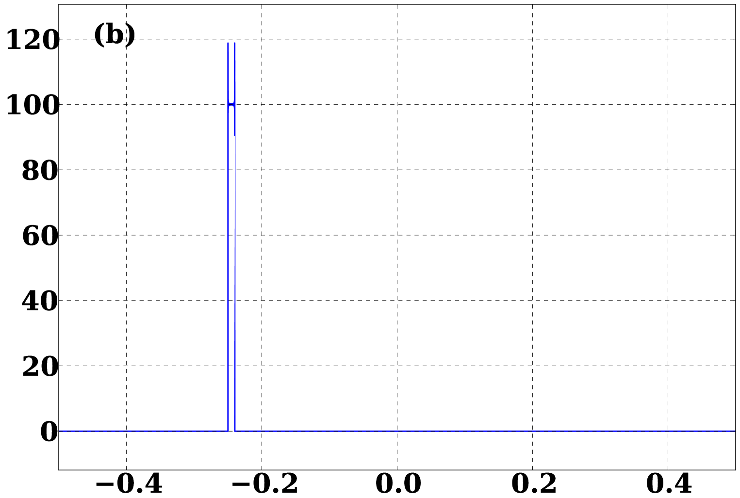
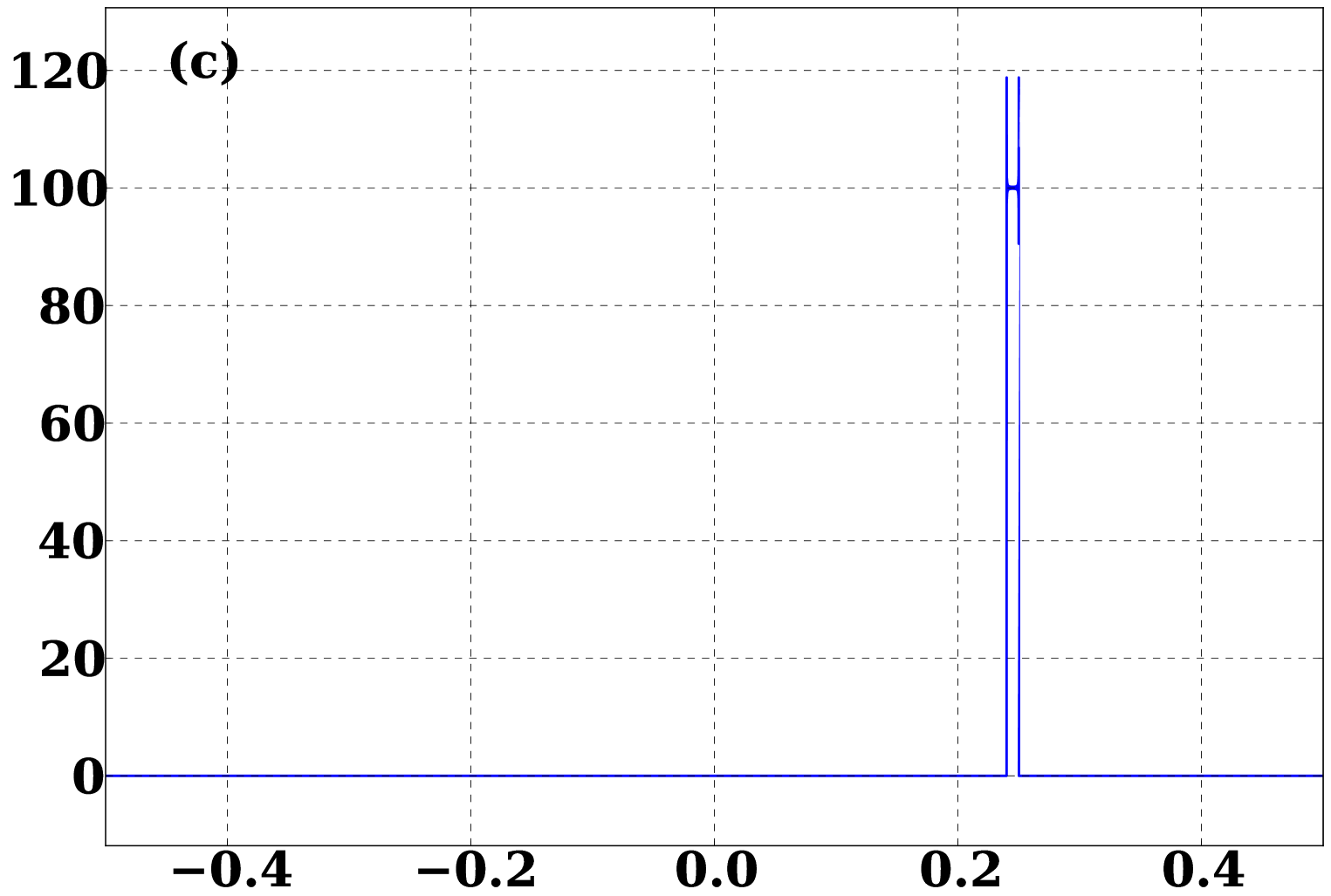
Figure 6: PMIC wave function plotted for time $N=50000$, with the values of (a) $t=0$ (b) $t=0.5T$, (c) $t=T$

One can observe the formation of rectangular wave functions at other values of $t$ as well. For instance, at regular time intervals of $\Delta t=0.1\;T$, we have observed that rectangular patterns appear. Some of these cases, where $t=0.1\;T$, $t=0.3\;T$, $t=0.7\;T$ and $t=0.9\;T$ show patterns as given in Fig. 7 (a) and in some other cases, where $t=0.2\;T$, $t=0.4\;T$, $t=0.6\;T$ and $t=0.8\;T$ the patterns are as shown in Fig. 7 (b). Similar calculations for other rational fractions of $T$ are also shown, such as $t=T/3$ in Fig. 7 (c), $t=T/4$ in Fig. 7 (d).

, , ,

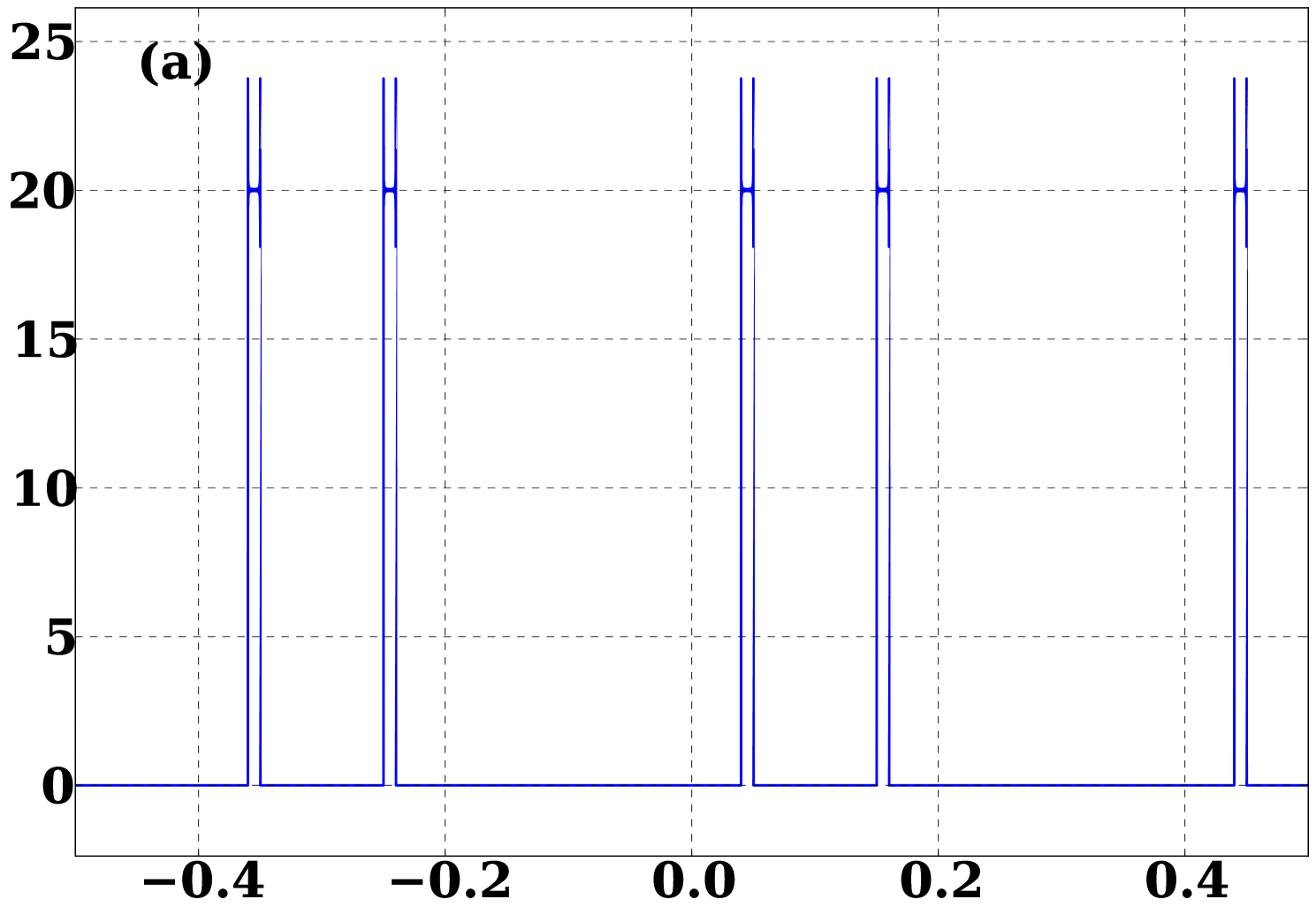
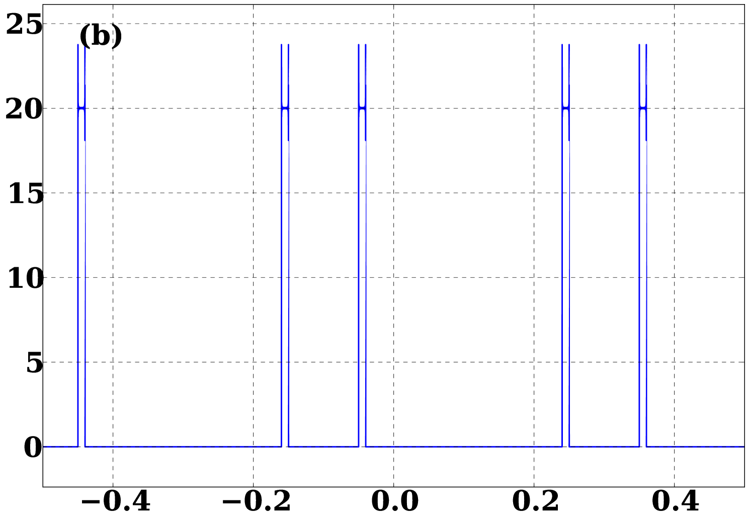
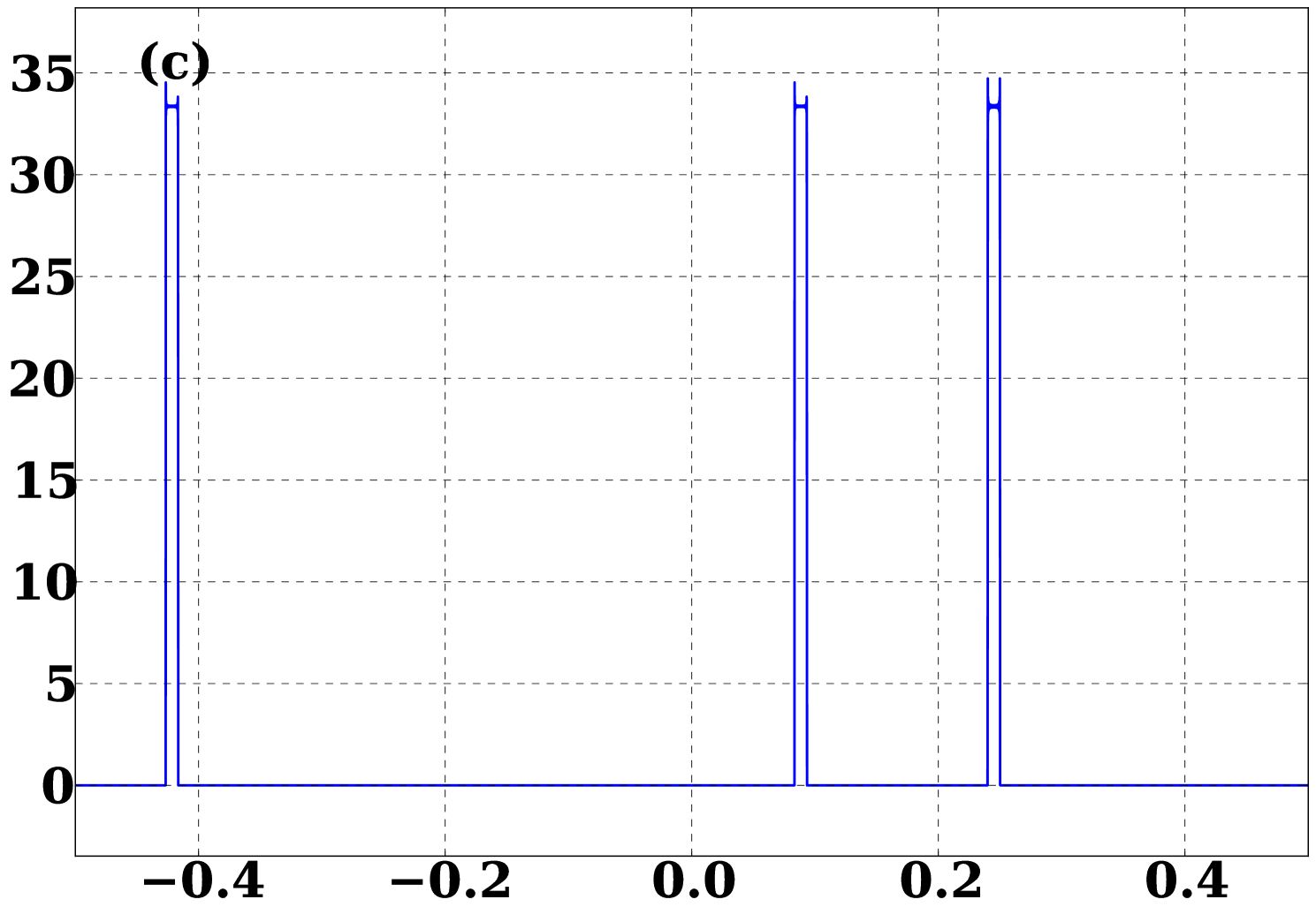
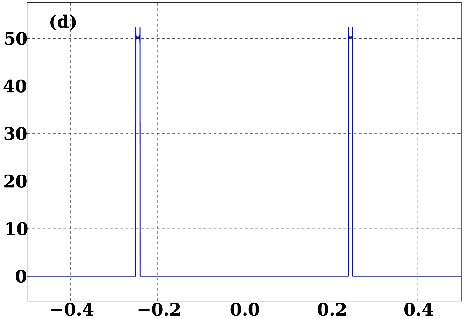
Figure 7: PMIC wave function plotted for time $N=50000$, with the values of (a) $t=0.1\;T$, $t=0.3\;T$, $t=0.7\;T$ and $t=0.9\;T$ (b) $t=0.2\;T$, $t=0.4\;T$, $t=0.6\;T$ and $t=0.8\;$ (c) $t=T/3\;$ (d) $t=T/4$

It was observed that the diffraction patterns are distinct only for $a\ll L$. As the value of the slit-width $a$ is increased, the Fraunhofer pattern appears somewhat late. But the revival time $T$ is independent of $a$. The most important feature to be noted is that the theoretically obtained patterns, especially those shown in Figs. 6 and 7, are testable in a diffraction experiment. The experiment proposed by us for testing these features is described in the next section.

4 Experimental set up

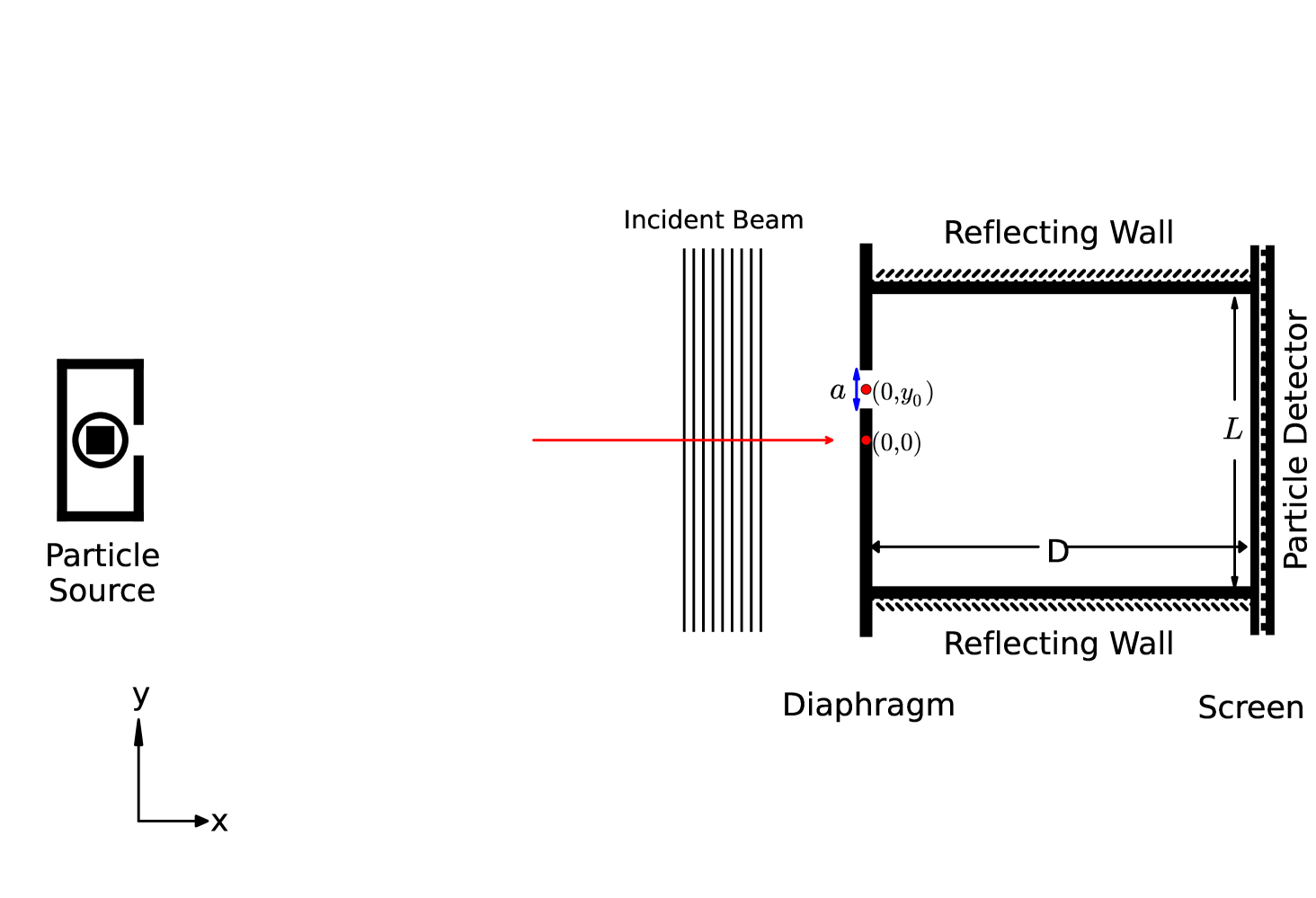
Figure 8: Experimental set up

In the above, PMIC patterns were obtained theoretically by following the standard axioms of quantum mechanics. Now we suggest a modified single-slit diffraction experiment to test these states.

The arrangement consists of a source from which a monoenergetic, collimated particle beam propagates parallel to the $x$-axis, in the positive direction. An impenetrable diaphragm of small thickness, which can at the same time absorb the particles hitting it, is placed at $x=0$. On the diaphragm, a slit of finite width $\Delta y=a$ with center at $y=y_{0}$ and of infinite length along the $z$-axis is cut. The location of the slit is thus given by $x=0$, $y_{0}-a/2\leq y\leq y_{0}+a/2$ and $-\infty<z<+\infty$. In between the diaphragm and a screen placed at $x=D$, again the potential is zero. But let there be two impenetrable and reflecting walls at $y=-L/2$ and $y=+L/2$, such that $y_{0}$ lies somewhere inside this interval. Thus a diffracted particle that passed through the slit can be considered to be confined to an infinite potential well along the $y$-direction. Just like the diaphragm, the screen is completely absorbing. Additionally, it serves to detect the particle, as in the case of experiments of diffraction and interference.

As per the geometry of the experimental set up, the particles are free in the region with $x<0$ and hence can be described by a plane wave advancing in the positive $x$-direction. This initial plane wave collapses when the particle passes the diaphragm at $t=0$. Since the particle that passed through the slit continues to be free along the $x$ and $z$-directions and is confined to an infinite potential well along the $y$-axis, the collapse is such that the product wave function of the particle for $t>0$ and $x>0$ can be written as

$$\Psi_{x}(x,t)\Psi_{y}^{y_{0},a}(y,t)=\frac{N\;e^{i(k_{x}x-E_{x}t/\hbar)}}{\sqrt{a}}\sum_{n}\left[\int_{y_{0}-a/2}^{y_{0}+a/2}dy^{\prime}\;u_{n}^{\star}(y^{\prime})\right]u_{n}(y)e^{-iE_{n}t/\hbar}.$$ (14)

Here $u_{n}$ and $E_{n}$ are given by Eqs. (12) and (13), respectively. The only affected component is the one along the the $y$-axis and it behaves as a PMIC wave function for $t>0$. Since $\Psi_{z}(z,t)$ always remains a constant, we have omitted this part in the product wave function.

The probability distribution corresponding to this total wave function is independent of $x$ and $z$; it depends only on $y$ and $t$. The problem of obtaining a stationary diffraction pattern on the screen can be solved if we assume trajectories along the $x$-direction, from the slit to the screen, as was done in [7]. The postulate of existence of particle trajectories, in addition to the standard postulates of quantum mechanics, is characteristic of nonlocal hidden variable theories such as the de Broglie-Bohm (dBB) [11], modified de Broglie-Bohm (MdBB) [12], and the Floyd-Faraggi-Matone (FFM) [13, 14, 15] trajectory formulations. In the present case, the $x$-component of velocity has the same value $v_{x}=\hbar k_{x}/m$ in all these three formalisms. Therefore we have taken the time with which a particle from the slit at $x=0$ reaches the screen placed at $x=D$ as $t=D/v_{x}$. Using this time $t$ in Eq. (14), one can plot $|\Psi_{x}(x,t)\Psi_{y}^{y_{0},a}(y,t)|^{2}$ against $y$ on the screen placed at a distance $D$. Actually, these are the same patterns with $|\Psi_{y}^{y_{0},a}(y,t)|^{2}$ plotted against $y$ in Fig. (1)-(7) discussed in Sec. 3, where $t=Dm/(\hbar k_{x})$. Predictions under this scheme are without any adjustable parameters and hence exact. In an actual experiment, obtaining those special patterns given in Fig. (2)-(5) may be possible with very good accuracy. Of particular interest is the occurrence of Fresnel and Fraunhofer patterns in this case. Moreover, it may be noted that since there exists a revival time $T$ for the wave function, the rectangular pattern will reappear at regular intervals as we vary $D$. The distance corresponding to the period with which it repeats is $D_{T}=\frac{4\hbar k_{x}}{\pi m}$. This is another clearly verifiable prediction of the theory.

5 Discussion

Here we treated the passing of the particle through a single-slit as the measurement of its position. A second measurement of the particle happens at the detector or screen, where it is completely absorbed. Our attempt was to study the time-evolution of the state of the system in between these two measurements. For that, we assumed that as a result of the first measurement, the plane wave function of the incident particle collapsed to a rectangular function, with a discontinuity at the edges of the slit. The attempt in [4] was to go to the momentum space and evaluate the probability distribution for the momentum variable. It is then tacitly assumed that the particles move towards the screen with the corresponding momentum values [5], as it would do in the case of classical mechanics. By this approach, only the Fraunhofer-type patterns were obtained on the screen, for all distances from the slit. In contrast, in [7] we postulated that the time-evolution of the collapsed state is described by the PMIC wave function. It was shown that this results in a single expression that describes the Fresnel and Fraunhofer diffraction.

In the present work, what we suggest is an experiment to test the PMIC state in a more precise way. The apparatus in our experiment is a modified version of Lloyd’s mirror in optics. The standard Lloyd’s mirror arrangement, which is originally designed to show interference [17], has only a primary source and its virtual image and no slits. In this form, the experiment is simpler than Young’s double-slit experiment, since the latter has the diffraction pattern due to two slits overlaid by an interference between the two sources. The Lloyd’s mirror can have only interference of light from two sources, and no slits. But our case discussed in this paper is similar to having two Lloyd’s mirrors, with a primary slit and an infinite number of virtual slits as sources. The repetition of rectangular pattern with the variation of $D$, as predicted by us using the PMIC formalism, is not anticipated in a wave optics treatment of this experiment. The verification of PMIC states by this experiment will be a step towards better understanding of ‘quantum collapse’ in general.

An important point that deserves serious attention is the value of $N$ used in the series expansion in Eqs. (7), (11) or (14). In practice, while plotting the wave function in the form of a converging infinite series, a finite upper limit for $n$ is unavoidable. We have put this upper limit in our calculations to be $N=50000$, so that a nearly rectangular function at $t=t_{M}$ is obtained. Any function can be written as a superposition of Dirac delta functions and it is well known that a delta function will be exact only when the limit $N\rightarrow\infty$ is taken in its closure representation. A problem related to the eigenstate of position is that the expectation value of energy shall tend to infinity. Consequently, the measurement of position with infinite precision is impossible. This is also true for wave functions with sharp discontinuities, such as the perfect rectangular wave function considered by us. A non-zero constant wave function inside the box, as considered in [8], requires infinite energy. However, physical objects such as the slit in this experiment will not have arbitrarily sharp boundaries and hence it is justifiable to fix a finite and large $N$ that corresponds to a moderately round edge. The energy-time uncertainty relation can also be invoked to justify a finite but very large value for $N$. In the experiment such as the diffraction through a single slit, the uncertainty in energy can be large but finite during the time of transit of the particle through the slit, which can be very small but nonzero. (The slit is assumed to be made on a thin diaphragm.) Moreover, since in this paper we are more concerned with the diffraction patterns, an upper limit for $N$ does not pose much problem because, as we have verified in Fig. 2, the shape of the curves have no appreciable change on further increasing the value of $N$. In particular, it may be noted that our main predictions, such as the Fraunhofer and Fresnel patterns, the reappearance of the rectangular patterns at particular values of distance $D$, etc. will remain unaffected even if we fix a finite, sufficiently large value for $N$.

In this paper we have also used the trajectory representation in quantum mechanics, which accept the existence of particle trajectories associated with the wave functions. In [7], we have used this additional postulate to obtain the single expression that gives a unified description of Fresnel and Fraunhofer diffractions. It was noted that all the three trajectory formulations make identical predictions in this case and that the success of our PMIC description supports the existence of particle trajectories. If verified, the predictions in this paper will also support the existence of particle trajectories.

References

- [1] Braginsky V B and Khalili F Y 1992 Quantum Measurement (New York: Cambridge University Press)
- [2] Wiseman H M and Milburn G J Quantum Measurement and Control (New York: Cambridge University Press)
- [3] Lamb W E 1969 Physics Today 22 23
- [4] Marcella T V 2002 Eur. J. Phys. 23 615
- [5] Rothman T and Boughn S 2011 Eur. J. Phys. 32 107
- [6] Fabbro B 2018 arXiv:1710.09758v4 [quant-ph]
- [7] John M V and Mathew K 2019 Found. Phys. 49 317
- [8] Berry M V 1996 J. Phys. A: Math. Gen. 29 6617
- [9] Tounli J, Alvarado A and Sanz A S 2019 Physica Scripta 94, 035202
- [10] Cohen-Tannoudji C, Diu B and Laloe F 1977 Quantum Mechanics vol.I (Paris: Hermann)
- [11] de Broglie L 1924 Ph.D. Thesis (University of Paris); de Broglie L 1927 J. Phys. Rad., 6e serie, t. 8 225
- [12] John M V 2002 Found. Phys. Lett. 15 329
- [13] Floyd E R 1982 Phys. Rev. D 26 1339
- [14] Faraggi A and Matone M 1999 Phys. Lett. B 450 34
- [15] Carroll R 2000 Quantum Theory, Deformation, and Integrability (Amsterdam: North Holland)
- [16] Arfken G B, Weber H J and Harris F E 2013 Mathematical Methods for Physicists, (Amsterdam: Elsevier)
- [17] Born M and Wolf E 2000 Principles of Optics (Cambridge: Cambridge University Press)