Cosmic Reionization

Abstract

The universe goes through several phase transitions during its formative stages. Cosmic reionization is the last of them, where ultraviolet and X-ray radiation escape from the first generations of galaxies heating and ionizing their surroundings and subsequently the entire intergalactic medium. There is strong observational evidence that cosmic reionization ended approximately one billion years after the Big Bang, but there are still uncertainties that will be clarified with upcoming optical, infrared, and radio facilities in the next decade. This article gives an introduction to the theoretical and observational aspects of cosmic reionization and discusses their role in our understanding of early galaxy formation and cosmology.

1 Historical Preface

Astronomers use distant objects as flashlights to peer through the vast space between galaxies, the so-called intergalactic medium (IGM). Intervening gas clouds absorb light in particular atomic transitions, producing an absorption spectrum, which can then be used to study the evolution of IGM properties throughout cosmic time. The first quasi-stellar objects (known as QSOs or quasars) were identified in 1960 by Rudolph Minkowski [1], Allan Sandage, and Maarten Schmidt [2]. They had star-like images, strong radio emission, and strangely placed, broad emission lines. Schmidt realized a few years later that the emission lines were actually hydrogen Balmer (principle quantum number $n\rightarrow 2$) series lines redshifted by 16% [3], who concluded that an extragalactic origin was the “most direct and least objectable” explanation. This realization sparked a flurry of research on QSOs [e.g. 4, 5, 6, 7], which were proposed to be powered by supermassive black holes (SMBHs) in 1964 by Edwin Salpeter [8] and Yakov Zel’dovich [9], and later associated with galactic nuclei by Donald Lynden-Bell [10] in 1969. These ideas were slowly accepted, but mounting evidence, especially with X-ray observations in the following decade [e.g. 11], confirmed the black hole paradigm.

James Gunn and Bruce Peterson [12] first realized in 1965 that even if a tiny fraction ($\sim 10^{-4}$) of the IGM was neutral it would absorb the QSO light blueward of the Ly$\alpha$ wavelength at 1216 Å ($n=1\rightarrow 2$). However when interpreting the most distant QSO at the time (redshifted by a factor of 2.01), there was no such absorption, strongly suggesting that the IGM was highly ionized when the universe was only one-quarter of its present age of 13.8 billion years.

Cosmic reionization is the process in which the IGM becomes ionized and heated. Now from many observations of the IGM and early galaxies, we know that reionization occurs everywhere in the IGM within a billion years after the Big Bang. As the first generations of galaxies fiercely form, they provide the necessary radiation to propel this cosmological event. Thus, it is informative to first overview some cosmological concepts and the astrophysics of photo-ionization in order to obtain a fuller understanding of reionization.

2 Background astrophysics

2.1 Cosmology

Cosmology is the study of the universe in its entirety. Large-scale galaxy surveys suggest that the universe follows the Cosmological Principle, stating the properties of the universe are the same for all observers when viewed at large enough scales (greater than 300 Mpc). In other words, the large-scale structure of the universe would be indistinguishable when traveling through space. At these scales, the universe is said to be isotropic and homogeneous. An isotropic universe means that there is no special direction in the universe, that is, it looks the same in all directions. A homogeneous universe is one with constant density and the distribution of galaxies is the same wherever the observer looks.

An isotropic and homogeneous universe can be treated as one entity. One can use general relativity to describe its dynamics, starting with the FLRW space-time metric,

$$ds^{2}=c^{2}dt^{2}-a^{2}(t)\left(\frac{dr^{2}}{1-Kr^{2}}+r^{2}d\Omega^{2}\right)$$ (1)

which results in an equation of motion describing its expansion or contraction. Here $ds$, $dt$, and $d\Omega$ are intervals of space-time, time, and angle, respectively, and $c$ is the speed of light. The variable $r$ is a spherical coordinate describing some observer and is not necessarily a distance measure between two observers. The curvature $K$ is a constant and can be either –1, 0, or +1, respectively corresponding to negative (elliptical), flat (Euclidean), and positive (hyperbolic) curvature of space.

The scale factor $a(t)$ denotes the expansion of the universe, where it is convention to take $a=1$ at the present day. In other words, when the universe had only expanded to half of its current size, $a=1/2$. The scale factor is also related to cosmological redshift $z=1/a-1$, which is common measure of distance and time in cosmology. A solution to the FLRW metric is the Friedmann equation

$$\left(\frac{\dot{a}}{a}\right)^{2}=H^{2}(t)=\frac{8\pi G}{3}\,\rho-\frac{Kc^{2}}{a^{2}}.$$ (2)

Here $H(t)$ is the Hubble parameter that describes the expansion (positive) or contraction (negative) rate of the universe. Edwin Hubble first discovered the expansion of the universe in 1927 by determining that more distant galaxies were receding at faster velocities. The present day value $H_{0}$ is thus usually given in units of km s^-1 Mpc^-1 that is the slope of this relationship.

The total mass-energy density $\rho=\rho_{m}+\rho_{r}+\rho_{\Lambda}$ of the universe comprises

• non-relativistic (cold) matter ($\rho_{m}\propto a^{-3}$) being geometrically diluted as space expands,

• radiation ($\rho_{r}\propto a^{-4}$) being both geometrically diluted and softened as its frequency is cosmologically redshifted, and

• vacuum energy, the so-called cosmological constant or dark energy, ($\rho_{\Lambda}\propto a^{0}$) that is pervasive and uniform throughout the universe.

It is useful to define the critical density $\rho_{\rm c}=3H_{0}^{2}/8\pi G$, which is obtained by solving for $\rho$ in Equation 2 after setting $K=0$. It is the dividing line between an open universe that expands forever and a closed universe that collapses onto itself.

Current constraints on the mass-energy components come from several experiments and sources—cosmic microwave background, supernovae, galaxy clusters, and large-scale structure. They have shown that the universe is flat ($K=0$), and about 69%, 26%, and 5% of the mass-energy is contained in dark energy, cold dark matter (DM), and baryons, respectively [13]. A small fraction ($9.3\times 10^{-5}$) is contained in radiation. These percentages of the $i$-th mass-energy component are always given in units of the critical density as $\Omega_{i}\equiv\rho_{i}/\rho_{\rm c}$: $(\Omega_{\Lambda},\Omega_{\rm c},\Omega_{\rm b},\Omega_{\rm r})\simeq(0.69,0.26,0.05,9.3\times 10^{-5})$. Unless otherwise stated, we assume these cosmological parameters in this article.

The Friedmann equation can be integrated to find that the scale factor $a$ or $(1+z)^{-1}$ is proportional to $t^{1/2}$ in a radiation-dominated universe, $t^{2/3}$ in a flat matter-dominated (the so-called Einstein-de Sitter, EdS) universe, and expands exponentially in a vacuum-dominated universe. The latest observational constraints suggest that the universe is flat and the cosmological constant exists ($\rho_{\Lambda}>0$), thus the scale factor $a(t)$ is monotonically increases with time, i.e. the universe is expanding and accelerating.

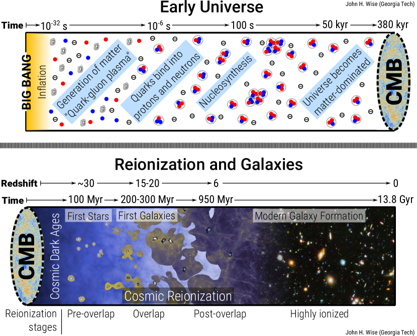
Figure 1: Cosmic timeline of the universe before (top) and after (bottom) recombination along with the stages of reionization. The galaxy survey image is taken from the Hubble Ultra Deep Field.

Knowing how the universe expands as a function of time, we also know how the mean temperature of the universe behaves, assuming it is filled with a perfect fluid. Starting from a hot Big Bang, the universe undergoes several phase transitions, where some are associated with the splitting of the four fundamental forces – gravity, strong, weak, and electromagnetic. All large-scale structures are seeded by quantum fluctuations that exponentially grew in size during the inflationary epoch ($t\sim 10^{-36}-10^{-32}\;\textrm{s}$ after the Big Bang) that eventually evolve into galaxies, shown in the cosmic timeline in Figure 1.

Along the way, one landmark cosmic event in the Universe occurred when gas transitioned from an ionized to a neutral state, known as either recombination or the surface of last scattering. Because the density of free electrons suddenly decreases, the photons become decoupled from matter and stream away, creating the cosmic microwave background (CMB).

After photons decouple, the universe at this time is a very dark and lonely place before stars or galaxies have formed. This epoch is sometimes referred to as the ’Dark Ages’ [14]. From this starless, neutral, and cold state, the entire universe will be gradually reionized by nascent galaxies and their constituents.

2.2 Large-Scale Structure

On small scales, the universe is neither isotropic nor homogeneous. One can look at our Milky Way and other galaxies just to see the inhomogeneity of matter. In the absence of light pollution, the dense stellar fields of the Milky Way, intertwined with dark dust lanes, stretch from horizon to horizon. Our galaxy is a very clumpy and active region in the universe, scattered with stellar clusters, cold molecular clouds, warm ionized regions, and hot supernova remnants.

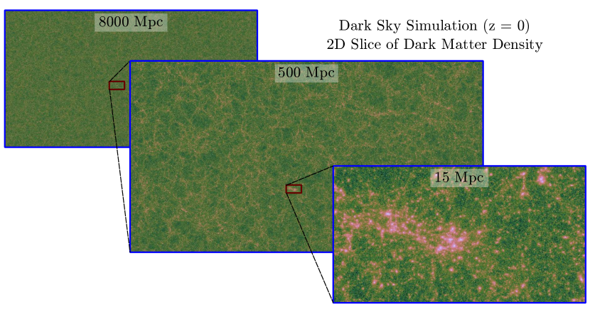
Figure 2: The Cosmic Web shown through slices of dark matter density in the Dark Sky Simulations [15] at the present-day. The fields of view in the left, center, and right panels are 8000, 500, and 15 Mpc. The universe is homogeneous and isotropic at scales above 300 Mpc but below which forms large-scale structures (clusters, filaments, walls, and voids).

On slightly larger scales, these ’island universes’ congregate in groups and clusters, containing dozens and hundreds of galaxies, respectively, which are connected to each other through long filaments. These cosmic connections form the cosmic web (see Figure 2) containing all cosmic structure: groups, clusters, superclusters, filaments, walls, and voids. When viewed in hundreds of Mpc, galaxy number densities become uniform, and web seems to repeat itself, suggesting the Cosmological Principle holds.

The cold dark matter (CDM) paradigm [16, 17, 18] explains cosmological large-scale structure extremely well, predicting galaxy number densities and their clustering to great accuracy. Because DM constitutes most of the matter in the universe, it controls the dynamics of large-scale structure. In any CDM cosmology, the building blocks are DM halos that have gravitationally collapsed and decoupled from the expansion of the universe. When a halo collapses, the dark matter and gas reaches equilibrium between the gravitational potential and its thermal and kinetic energy [19]. In equilibrium, one can use a spherically symmetric halo collapsing in an expanding universe to find that its mean density of $18\pi^{2}$ times the critical density $\rho_{\rm c}$ at the collapse time [20]. Recall that the density changes with $a^{-3}=(1+z)^{3}$ from cosmological effects. Given a halo mass $M_{\rm h}$ and the halo mean density $\rho_{\rm h}=18\pi^{2}\rho_{\rm c}(1+z)^{3}$, three halo properties can be derived.

1. Assuming a spherical halo, we compute the halo radius by dividing the halo mass by the mean density, giving the volume, and we then solve for the radius,

   $$r_{\rm h}=\left[\frac{M_{\rm h}}{(4\pi/3)\rho_{\rm h}(1+z)^{3}}\right]^{1/3}.$$ (3)

2. The kinematics of stars and gas within a halo can be better understood by relating their velocities to the value that results in circular motion, the circular velocity of a system,

   $$V_{\rm c}=\sqrt{\frac{GM_{\rm h}}{r_{\rm h}}}.$$ (4)

3. As the halo collapses, the gravitational potential energy can be converted into thermal energy and an equivalent temperature, which is termed the virial temperature. We can calculate it by equating the kinetic energy, $mV_{\rm c}^{2}/2$, of a typical gas particle (usually hydrogen) with mass $m$ in a circular orbit with its thermal energy, $k_{\rm b}T_{\rm vir}$, resulting in

   $$T_{\rm vir}=\frac{mV_{\rm c}^{2}}{2k_{\rm b}}$$ (5)

CDM structure forms hierarchically with objects growing through a series of halo mergers. Galaxies exist at the centers of DM halos and are along for the ride throughout mergers, sparking galaxy interactions and mergers.

In this review, we are interested in the galaxies that form inside these halos, asking ourselves the question: How frequently do stars and galaxies form in the early universe, and generally when do they form? For a halo to host star formation, the gas must be able to cool and condense through some radiative process. Catastrophic cooling and collapse occurs when a halo reaches some critical temperature $T_{\rm vir}$ and associated mass $M_{\rm h}$. From these critical points, we can estimate the abundance of the first stars and galaxies as a function of time. Their radiation will permeate the IGM, photoionizing and photoheating it. To study reionization from first principles point of view, we next overview the basic physics of photo-ionization.

2.3 Ionization and recombination

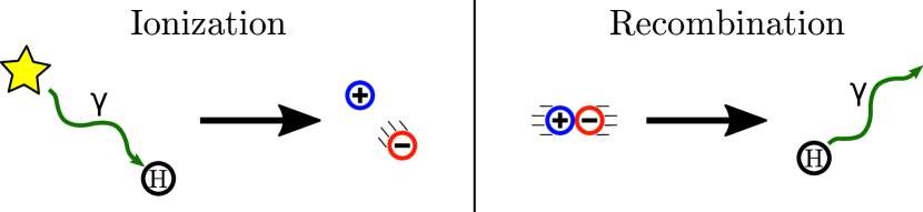
Figure 3: Cosmic reionization is governed by individual ionization (left) and recombination (right) events. Photons above 13.6 eV will ionize neutral hydrogen, creating a free electron and proton. Recombination occurs more often at lower temperatures ($T<10^{4}~{}\mathrm{K}$) when these particles combine back into neutral hydrogen. This produces a photon with 13.6 eV plus any excess energy from the particles’ kinetic energy.

The radiation from the first luminous objects will ionize and heat the surrounding IGM once it escapes from their host halos. These are known as cosmological H ii regions. The ionization and recombination of hydrogen atoms ($\mathrm{H}+\gamma\leftrightarrow\textrm{H}^{+}+\textrm{e}^{-}$) are dominant processes in H ii regions and are illustrated in the Figure 3. Ionizations occur when photons with energies $E>I_{\rm H}=13.6\;\textrm{eV}$ interact with neutral hydrogen atoms, where their excess energies are subsequently thermalized. Recombinations occur when the Coulomb force attracts protons and electrons, which becomes efficient at temperatures $T\leq 10^{4}\;\textrm{K}$. One recombination releases a photon with an energy that is the sum of the kinetic energy of the electron and binding energy of the quantum state, $I_{\rm H}/n^{2}$. If the electron recombines into an excited state ($n>1$), the electron will quickly decay into the ground state in a series of transitions.

In a region with ionizing radiation, the gas approaches ionization balance with the recombination rate equaling the ionization rate. We can equate these two rates and solve for the ionization fraction $x_{e}\equiv n_{\rm e}/n_{\rm H}$ of the gas at equilibrium. Here $n_{\rm e}$ and $n_{\rm H}$ are the electron and hydrogen number density, respectively.

To calculate the recombination rate, we can make the following assumptions: (i) the rate will be proportional to the product of the number density of protons $n_{\rm p}$ and electrons $n_{\rm e}$, (ii) the gas is pure hydrogen, giving $n_{\rm p}=n_{\rm e}$, and (iii) the rate depends on the temperature and into which quantum state $n$ it recombines. There are two rates associated with recombination:

Case A:

This rate is the sum of recombination rates into all electronic levels. However if an electron recombines directly into the ground state, this will release a photon that can ionize another hydrogen atom, which is not the case if it recombines into an excited state. Effectively, there are zero net recombinations in this case, and we can ignore the $n=1$ recombination rate.

Case B:

This rate is the sum of recombination rates into all excited states, ignoring the ground state for reasons recently stated. It is also known as the “on-the-spot” approximation and is the appropriate one to use in the ionization balance problem.

The ionization rate can be calculated given some ionizing radiation flux. Photons will be absorbed as they travel through a medium with a neutral hydrogen number density, and the probability for a single absorption is quantified by the photoionization cross-section $\sigma_{\rm HI}\approx 6.8\times 10^{-18}(E/13.6\;\textrm{eV})^{-3}\;\textrm{cm}^{2}$ that decreases with photon energy. The cross-section is zero below 13.6 eV because the photon does not have sufficient energy to ionize hydrogen.

By equating the recombination and ionization rates, we can show that H ii regions are highly ionized, having ionization fractions nearly equal to one and neutral hydrogen fractions around $10^{-4}$. They are thus well described by a fully ionized plasma. The ionization flux, however, decreases as the distance squared from the star, resulting in the medium being the most ionized near radiation sources with it decreases rapidly with increasing distance.

2.4 Evolution of an H ii region

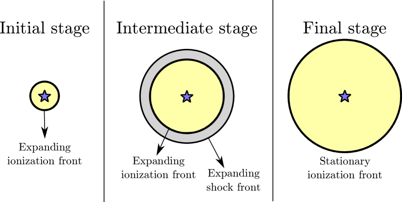
Figure 4: Three stages of H ii region evolution. Left: After a massive star forms, its UV radiation ionizes and heats the nearby interstellar medium, creating an H ii region. Middle: After some time, the heated region expands and drives an outgoing shock (middle), carrying gas away from the star. Right: The H ii region comes into pressure equilibrium with the ambient medium.

A radiation source can only provide a finite number of ionizing photons per second, so there must be some limit of ionizations possible in the surrounding region. Recombinations are happening concurrently with ionizations in the highly ionized H ii region. In some radial direction, if all of the ionizing photons are absorbed by newly recombined atoms inside the H ii region, there will be no more flux left at the ionization front. When this happens, the front stalls out and reaches an equilibrium [21]. We can determine the radius of the H ii region $R_{\rm s}$, known as the Strömgren radius, by balancing the total number of ionizations and recombinations in a region. Assuming spherical symmetry and a static and uniform medium, we set these total numbers to be equal and solve for the radius. It is larger for more luminous sources (higher ionization rates) and for ambient gas with smaller densities (lower recombination rates).

Figure 4 depicts the evolution of an H ii region from when the star first ignites to the final stage when the ionization front stalls out. Initially the newborn star is surrounded by a dense medium from which it formed. The radiation front travels near the speed of light at early times through this dense gas, where the recombination rate is high. The H ii region is now heated to over 10,000 K and is encompassed by a cold ambient medium. The gas thus has a higher pressure than its surroundings and will start to expand. This marks the transition from the initial stage to the intermediate stage after the time it takes a sound wave to cross the H ii region. As the material is forced away from the star by the high pressure gas, it shocks with the ambient medium. The shock wave “sweeps up” most of the gas in its path and accumulates mass, leaving behind a more diffuse gas within the H ii region. As the density decreases, the recombination rate decreases accordingly. Thus, the Strömgren radius increases with time. Eventually the the H ii region comes into pressure equilibrium with the ambient medium, and both the shock front and ionization front stall out at the final Strömgren radius. This final equilibrium usually takes hundreds of millions of years to manifest, which is much longer than the lifetimes of massive stars, suggesting that this final stage is usually not realized in nature.

More relevant for reionization, this scenario of a central source ionizing its surrounding neutral gas can be extended to whole galaxies. Any ionizing radiation that escapes from the galaxy will create a cosmological H ii region that is the building block of reionization.

3 Ending the Cosmic Dark Ages

Cosmic reionization involves the coupling of non-linear physics of galaxy formation with the non-local physics of gravity and radiation transport to produce a global phase transition. Reionization is completely different from the local nature of the earlier phase transitions that only depend on the thermal state of the plasma. The mixture of small- and large-scale physics makes for a complex problem. Some important questions to ask about cosmic reionization are: What are the main sources of reionization? When does reionization begin and end? What is the topology of the ionized regions? What can be learned about early galaxies from reionization and vice-versa? How does reionization affect galaxy formation?

The present-day IGM has a mean temperature around $10^{5}\;\textrm{K}$ and the primordial elements of hydrogen and helium are near complete ionization [e.g. 22]. Maintaining this relatively high temperature and ionization state is an ultraviolet and X-ray radiation background, sourced by countless galaxies and their central black holes [23]. But how did the IGM become ionized and heated in the first place?

This becomes a particularly rich question when combined with the fact that galaxies were first assembling during the epoch of reionization (EoR). Depending on their mass, DM halos can support the formation of various types of galaxies during the epoch of reionization, shown in Figure 5. As halos grow with time, their gravitational potentials deepen, and their gaseous components shock to higher virial temperatures $T_{\rm vir}$. The shocked gas undergoes various radiative processes, cooling the gas. Cold, dense gas fuels star formation and is a good tracer of its strength. Several physical processes control the amount of cold dense gas, but two key processes are the (1) efficiency of radiative cooling and (2) the ability of the halo to retain gas that is heated by radiation and supernovae. They are both directly related to the halo mass. Thus, we can categorize halos by their mass and associate different types of behavior with them.

• Very weak cooling and no star formation (Section 3.1) below $\sim$$3\times 10^{5}~{}{\textrm{M}_{\odot}}$;

• The first generations of massive primordial stars (Section 3.2) that are sparked by H₂ cooling in halos with masses between $3\times 10^{5}~{}{\textrm{M}_{\odot}}$ and $10^{7}~{}{\textrm{M}_{\odot}}$;

• The first generations of galaxies (Section 3.3) that form stars efficiently but its gas is susceptible to being blown out of the shallow gravitational potential in halos of masses between $10^{7}~{}{\textrm{M}_{\odot}}$ and $3\times 10^{9}~{}{\textrm{M}_{\odot}}$;

• More “normal” galaxies that exist in more massive halos. They are reminiscent of a subset of present-day galaxies with strong star formation, is resistant to major gas losses, and may contain a central BH.

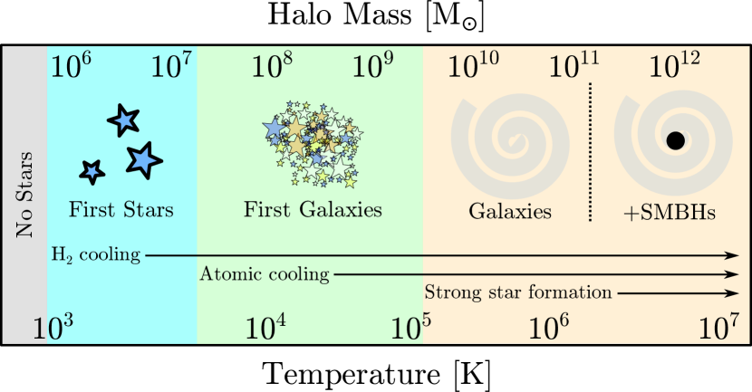
Figure 5: Below $10^{5.5}~{}{\textrm{M}_{\odot}}$, halos cannot host cold gas and stars. As halos grow, they can host increasingly more cold gas and fuel stronger star formation, ranging from metal-free massive stars ($10^{5.5}-10^{7}~{}{\textrm{M}_{\odot}}$) to the first generation of galaxies ($10^{7}-10^{9.5}~{}{\textrm{M}_{\odot}}$) to more massive galaxies and supermassive black holes ($>10^{9.5}~{}{\textrm{M}_{\odot}}$).

These star forming halos all contribute to cosmic reionization, which can be divided into three phases [24]—pre-overlap, overlap, and post-overlap—that describe the connectivity of the cosmological H ii regions, illustrated in Figure 1. In the pre-overlap phase, each galaxy produces its own H ii region as it forms. These regions are divided by a vast neutral IGM, and their evolution can be treated independently, only requiring the escaping ionizing luminosity of the central galaxy. In the overlap phase, these regions start to combine with nearby regions [25]. Multiple galaxies can contribute to the UV emissivity that pervades the ionized region, dramatically increasing the mean free path of ionizing photons and accelerating the reionization process. Finally in the post-overlap phase, most of the IGM is ionized with some neutral patches remaining the universe. These neutral regions erode away as ionization fronts created from the UVB propagate into these vestiges of an earlier cosmic time.

3.1 The Dark Ages

The Cosmic Dark Ages began after recombination at $z\sim 1090$ (380,000 years after the Big Bang) and lasted until the first stars and galaxies started to light up the universe hundreds of millions of years later. However first, it is worthwhile to discuss the supersonic relative velocities between DM and gas that arises before and during recombination. The importance of this phenomenon was overlooked until recently [26]. Before recombination, free electrons scatter off photons, strongly coupling the gas and radiation, but the collisionless DM is not affected by this coupling. These two components of the universe thus had different velocities as radiation and gas decoupled at recombination. The root-mean-square value at this time was $\sim 30{{\;\rm km~{}s^{-1}}}$ and fluctuated on comoving scales between $\sim 3-200$ Mpc. Thus on comoving scales of $\sim$Mpc, the gas has a uniform bulk velocity relative to DM. This so-called streaming velocity decayed as $a^{-1}$, remained supersonic throughout the Dark Ages, and prevented gas from collecting in the potential wells of the smallest DM halos that would have otherwise formed stars.

The mean gas temperature of the universe after recombination is tightly coupled to the CMB temperature through Compton scattering until a redshift $z_{\rm t}\approx 136$ at which time $T=2.73\;\textrm{K}(1+z_{\rm t})=374\;\textrm{K}$ [27], where 2.73 K is the current CMB temperature $T_{\rm CMB,0}$. Afterwards in the absence of any heating, the IGM in an expanding universe cools adiabatically with its temperature decreasing proportionality to $a^{-2}$, or equivalently $(1+z)^{2}$. Throughout this epoch, DM halos are continually assembling, but the gas cannot collapse into these halos because of this excess thermal energy and kinetic energy from streaming velocities. The Jeans mass

$$M_{\rm J}=\frac{\pi^{5/2}}{6}\frac{c_{\rm s}^{3}}{(G^{3}\rho)^{1/2}}$$ (6)

describes the required mass of an object that has enough gravity to overcome thermal pressure, inducing a collapse. Here $\rho$ and $c_{\rm s}=(\gamma k_{\rm B}T/\mu m_{\rm p})^{1/2}$ are the gas density and sound speed, respectively. Using the IGM temperature $T_{\rm gas}$ and the mean gas density $\bar{\rho}_{\rm b}=\rho_{c}\Omega_{b}(1+z)^{3}$, one can calculate the cosmological Jeans mass $M_{\rm J}$ that is around $32{,}000~{}{\textrm{M}_{\odot}}$ at $z=30$ (100 Myr after the Big Bang) and changes as $a^{-3/2}$. It provides an estimate of the minimum halo mass that can collect baryonic overdensities [28] in the case without streaming velocities.

3.2 The first stars

Historically, astronomers have categorized stars by their metallicity – Population I for stars like our Sun, which has 1.3% metals by mass [29], and Population II for stars with metallicities less than 1/10^th of the solar metallicity fraction. However, the Big Bang only produced hydrogen, helium and trace amounts of lithium. So there must have been an initial population of stars composed of these light elements, whose supernovae enrich later generations of stars with metals that we observe today.

This first generation of stars, known as Population III (Pop III), is inherently different than present-day stars because they form in a neutral, pristine, untouched environment from a primordial mix of hydrogen and helium. Being metal-free reduces the cooling ability of the collapsing birth cloud, resulting in stars that are typically more massive than nearby stars [e.g. 30, 31].

Metal-free gas loses most of its thermal energy through H₂ formation in the gas-phase, using free electrons as a catalyst, in the following reactions.

$$\textrm{H}+\textrm{e}^{-} \rightarrow \textrm{H}^{-}+\gamma$$ (7)

$$\textrm{H}^{-}+\textrm{H} \rightarrow \textrm{H}_{2}+\textrm{e}^{-}$$ (8)

Recombination leaves behind a residual free electron fraction on the order of $10^{-5}$. As gas falls into the halos, it shock-heats to around the virial temperature $T_{\rm vir}$, and its electron fraction is slightly amplified.

But H₂ is a fragile molecule that can be dissociated in the Lyman-Werner (LW) bands between 11.1 and 13.6 eV at soft UV wavelengths where the universe is optically thin. Furthermore, the intermediary product H^- can be destroyed through the photo-detachment of the extra electron that has an ionization potential of 0.76 eV in the infrared. Accordingly, the timing and host halo masses of Pop III star formation is dependent on the preceding star formation that produces the soft UV and infrared radiation backgrounds. The minimum halo mass that can support sufficient H₂ formation that can induce a catastrophic collapse is around $10^{5}~{}{\textrm{M}_{\odot}}$ in the absence of LW radiation but steadily increases to $10^{7}~{}{\textrm{M}_{\odot}}$ in strong LW radiation fields [32]. Additionally, streaming velocities can suppress Pop III star formation in halos with masses $M\lower 3.00003pt\hbox{$\,\buildrel<\over{\sim}\,$}10^{6}{\textrm{M}_{\odot}}$ with its exact value depending on the local streaming velocity magnitude that varies on scales of tens of Mpc [e.g. 33, 34].

Simulations of the first stars and galaxies that consider a LW background have found that Pop III stars form at a nearly constant rate of $\sim 3\times 10^{-5}$ M_⊙ yr^-1 Mpc^-3 until the end of reionization [e.g. 35]. Each star produces a tremendous amount of ionizing radiation because they are thought to be massive with characteristic masses of tens of solar masses [e.g. 36], some forming in binary systems and small clusters [e.g. 37, 38]. They have effective surface temperatures $\sim 10^{5}\;\textrm{K}$ that is approximately mass-independent above 20 M_⊙ because of the lack of typical opacities associated with metals in their photospheres. They live for 3–10 Myr and produce between $2\times 10^{48}$ and $10^{50}$ hydrogen ionizing photons per second in the mass range 15–100 M_⊙[39]. Most of these photons escape into the nearby IGM, and the averaged escape fraction $f_{\rm esc}$ increases from 20% for a single 15 M_⊙ star to nearly 90% for a single 200 M_⊙ star [40]. The exact values of $f_{\rm esc}$ will depend on the total Pop III stellar mass in the halo, the halo mass, and its gas fraction. After their main sequence, some explode in supernova, chemically enriching the surrounding few proper kpc, where the exact fraction depends on their uncertain their initial mass function. Because of this strong feedback, they quench their own formation, blowing out most of the gas that originally existed in their host halos. Furthermore once the medium is enriched with metals, it’s ’game over’ for Pop III stars in affected regions because by definition, they are metal-free.

3.3 The first galaxies

These heavy elements set the stage for the first galaxies that form in larger halos, in which atomic (Ly$\alpha$) line cooling is efficient. Accordingly, these halos are known as atomic cooling halos and have virial temperatures above $\sim$8000 K. These pre-galactic halos are generally gas-poor ($f_{\rm gas}\equiv M_{\rm gas}/M_{\rm vir}\simeq 0.05-0.10$) because they are recovering from the gas blowout that their halo progenitors experienced. If the halo is below the atomic cooling limit, star formation is bursty but still intense during active periods, forming between $10^{4}$ and $10^{5}~{}{\textrm{M}_{\odot}}$ of stars before they can cool efficiently through atomic hydrogen transitions. They have star formation rates $\dot{M}_{\star}$ between $10^{-4}$ and $10^{-3}$ M_⊙ yr^-1, doubling their stellar masses $M_{\star}$ every $\sim 30\;\textrm{Myr}$ (corresponding to a specific star formation rate, $\mathrm{sSFR}\equiv\dot{M}_{\star}/M_{\star}\sim 3\times 10^{-8}\;\textrm{yr}^{-1}$), and producing $\sim 3\times 10^{49}$ ionizing photons per second. After the halo crosses the atomic cooling limit, it can form stars in a continuous fashion at $\mathrm{sSFR}\sim 3\times 10^{-8}\;\textrm{yr}^{-1}$, which can vary by an order of magnitude from galaxy to galaxy, depending on how it has been affected by feedback from previous star formation [e.g. 41, 42, 43]. By the time the halo mass reaches $10^{9}~{}{\textrm{M}_{\odot}}$, the first generations of galaxies contain between $10^{6}$ and $10^{7}~{}{\textrm{M}_{\odot}}$ of metal-poor ($Z\lower 3.00003pt\hbox{$\,\buildrel<\over{\sim}\,$}0.1~{}{\rm\,Z_{\odot}}$) stars.

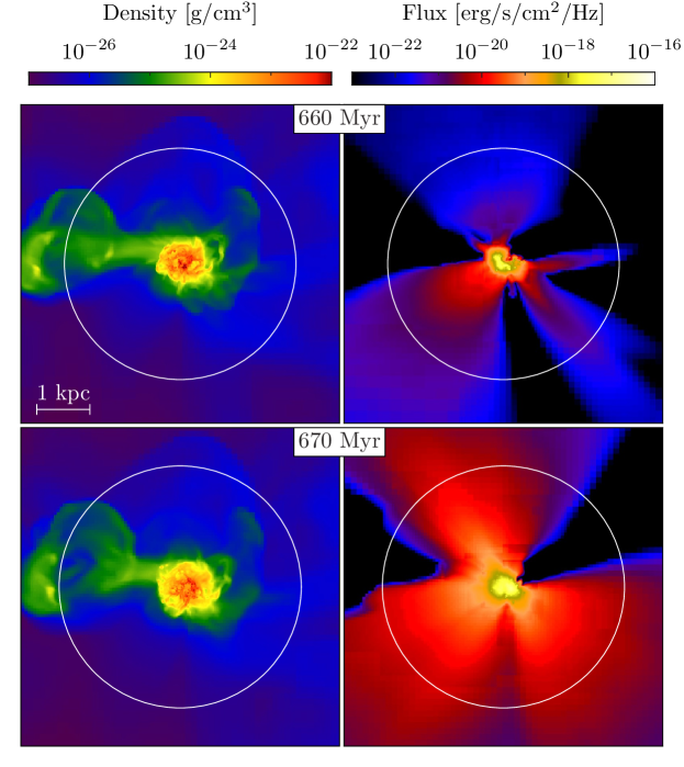
Figure 6: Projections of gas density (left) and UV radiation flux (right) of a first generation galaxy with a stellar mass $\sim 10^{5}{\textrm{M}_{\odot}}$ at redshift $z\simeq 8$ with the bottom panels pictured 10 Myr after the top panels. The white circle marks the virial radius. The UV escape fractions are 1% (top) and 7% (bottom). Adapted from [44].

An important quantity in reionization calculations is the UV escape fraction $f_{\rm esc}$, which is notoriously difficult to observationally measure and to theoretically calculate. Most reionization models find that $f_{\rm esc}=0.05-0.2$, independent of halo mass, generally produce reasonable reionization histories [e.g. 45]. In the past decade, there have been great strides in the development of radiation hydrodynamics simulations of the first galaxies in which a direct calculation of $f_{\rm esc}$ is feasible. This fraction is highly variable from galaxy to galaxy, and even in a single object, it can vary from nearly zero to unity over its formation sequence (see Figure 6). Because the interstellar medium (ISM) is clumpy, the ionization fronts propagate outwards toward to the IGM at varying velocities with respect to angle. The ionizing radiation generally escapes in the directions with small neutral column densities. Once an ionized channel is opened between a star cluster and the IGM, it remains ionized as long as massive stars remain alive. Thus, the value of $f_{\rm esc}$ can be thought as the solid angular fraction that the ionized channels cover. Such efforts have found that the smallest galaxies have high escape fractions. The median time-averaged value of $f_{\rm esc}$ is $\sim 0.5$ in halos with masses $M_{\rm vir}\simeq 10^{7}~{}{\textrm{M}_{\odot}}$, and it decreases to 0.05–0.10 at $M_{\rm vir}\simeq 10^{8}~{}{\textrm{M}_{\odot}}$ [41, 46, 43]. When the total escaping photons are integrated over all galaxies, half of the photon budget to reionization originate from halos with $M_{\rm vir}\lower 3.00003pt\hbox{$\,\buildrel<\over{\sim}\,$}10^{9}~{}{\textrm{M}_{\odot}}$.

3.4 The first black holes

Black holes grow through mergers of two black holes and the accretion of gas. The latter is the primary growth mechanism, where material falls down the deep gravitational potential well. It forms an accretion disk orbiting around the black hole because of conservation of angular momentum. Eventually, gas migrates to increasingly smaller radii and falls into the black hole. In the process, the gas is heated intensely from the strong gravity field and emits radiation. Any outward radiation interacts with the inflowing gas, which can suppress the growth rate of the black hole.

Because Pop III stars are thought to be massive, a large fraction will leave a black hole remnant. Temperatures in accretion disks around stellar-mass black holes are between $10^{4}$ and $10^{7}\;\textrm{K}$ and thus emits strongly in the hard UV and X-ray energies. Their UV luminosities are insignificant when compared to stellar sources, but their X-rays should have an impact on the thermal and ionization state of the IGM. These high energy photons can penetrate much deeper into the IGM, creating large partially ionized regions with $x_{e}=0.01-0.02$ out to distances of 100 kpc [47], creating a much different reionization topology than stellar sources [48].

Pop III stars leave behind some of the first black holes in the universe. These could be the “seeds” for more massive black holes that we observe in the nearby Universe. They can possibly grow to supermassive black holes that are millions and sometimes billions of times more massive than our Sun. The most extreme cases have masses over $10^{9}~{}{\textrm{M}_{\odot}}$ at redshifts $z>6$ when the universe was younger than 800 million years old [49]. The formation and growth of black holes are still active research topics. A few pressing questions are: How did massive black holes in the distant universe grow so rapidly? Did their radiation contribute to reionization? How often did stellar-mass black holes grow into supermassive black holes? Where are these stellar remnants today? Observations from the epoch of reionization will provide us with clues in order to solve these mysteries.

4 Constraints from the Edge of the Observable Universe

Now that we have covered the basic astrophysics and the theoretical aspects of reionization, we can gain insight on cosmic reionization through some key observations. There are various independent probes of reionization, either measuring the ionization and thermal state of the IGM or the properties of galaxies forming during the EoR. The vast majority of these observations are difficult with the photons streaming across the observable universe to Earth, requiring long exposure times and/or large telescopes. Here we cover the basic physics behind each method and the latest constraints.

4.1 QSO Spectra

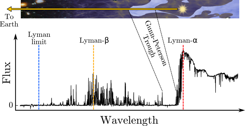
Figure 7: Light from distant quasars, powered by supermassive black holes, can probe the ionization and thermal state intergalactic medium. Overdense clumps of intergalactic gas absorb some fraction of light from the intrinsic spectrum (bottom) when the photons ionize any neutral hydrogen. Only lines in the Lyman series, down to the Lyman limit (912 Å), with Ly$\alpha$ (1215 Å) and Ly$\beta$ (1026 Å) being the strongest. Absorption lines from clouds at various redshifts create a Ly$\alpha$ forest. When these lines becomes numerous enough, it creates a Gunn-Peterson trough that is indicative of an elevated neutral hydrogen fraction and the end of the Epoch of Reionization.

Light from distant QSOs can be used as flashlights to probe the intervening IGM. Neutral gas clouds at some redshift $z_{\rm abs}$ will strongly absorb light at the Lyman-$\alpha$ wavelength $\lambda_{\alpha}=1216\;\textrm{\AA}$ in its rest frame that is then redshifted to a wavelength $\lambda_{\alpha}(1+z_{\rm abs})$ in observations. The schematic and accompanying spectrum in Figure 7 depicts this technique of quasar absorption spectra mapping out the IGM. It shows that many gas clouds at varying redshifts between the QSO and us has blocked out much of the radiation at wavelengths shorter than $\lambda_{\alpha}$.

As discussed previously, Gunn and Peterson used QSO spectra to determine that the IGM must be highly ionized, otherwise an absorption trough, now termed the Gunn-Peterson (GP) trough, would have been present at $\lambda_{\alpha}<1216\;\textrm{\AA}$. The optical depth to Ly$\alpha$ photons ($n=1\rightarrow 2$) is extremely high, upwards of $10^{5}$ in a completely neutral IGM at high redshifts. Because optical depth is proportional to neutral hydrogen density, the IGM even with a tiny neutral fraction $f_{\rm HI}\equiv n_{\rm HI}/n_{\rm H}\sim 10^{-4}$ will be optically thick to Ly$\alpha$ photons and absorb all light at a wavelength $1216(1+z_{\rm abs})$ Å. Because Ly$\alpha$ is such an effective absorber, this method only probes the neutral fraction of highly ionized gas and cannot be used to peer into the EoR.

There have been dozens of $z\geq 6$ QSO absorption spectra that have GP troughs [50], which are increasingly opaque with redshift. This is a strong constraint that cosmic reionization is complete by $z\sim 6$. The IGM near QSOs are also exposed to a strong radiation field and should be more ionized than the typical IGM. This is known as the proximity effect, resulting in weaker absorption between the Ly$\alpha$ emission line and GP trough. The sizes of these ionized regions are on the order of tens of Mpc at $z\sim 6$ [e.g. 51]. Similar to this type of analysis, absorption from a partially ionized IGM in the proximity zone will produce a damping Ly$\alpha$ wing that occurs when the neutral column density $N_{\rm HI}\lower 3.00003pt\hbox{$\,\buildrel>\over{\sim}\,$}10^{20}\;\textrm{cm}^{-2}$. The spectrum of one of the most distant QSOs at $z=7.08$ constrains the ionized fraction to be $x_{\rm e}\simeq 0.60$ at this redshift [52]. On the opposite end, there are still some neutral islands with sizes up to 160 Mpc at $z=5.5-6$ [53], but they quickly erode as the increasing UV background ionizes them [50], showing that cosmic reionization is an inhomogeneous process.

4.2 The Ly$\alpha$ forest

The Ly$\alpha$ forest denotes the myriad of Ly$\alpha$ narrow absorption lines coming from clouds in the IGM between the quasar and us. For a cloud existing at a redshift $z$, they will create an absorption line at wavelength $1215(1+z)$Å. They become more abundant with increasing redshift [54] and probe clouds with column densities $\log(N_{\rm HI}/\textrm{cm}^{-2})=12-16$. These lines become so abundant that they start to block out all of the background light, transforming into a GP trough at $z\sim 6$. The example spectrum in Figure 7 shows a dense Ly$\alpha$ forest, transmitting very little light at wavelengths between Ly$\alpha$ and Ly$\beta$ (1026 Å). This particular spectrum transmits more light at shorter wavelengths, or equivalently, lower redshifts, suggesting that this line of sight is becoming more ionized with decreasing redshift. One constraint on the ionized fraction is the ’dark fraction’ of QSO spectra in the Ly$\alpha$ forest that originate from either neutral patches or residual neutral hydrogen in ionized regions [55]. Taken at $z=5.9$, the dark fraction in the Ly$\alpha$ forest results in an lower limit of $x_{\rm e}>0.94$ [56].

Because Ly$\alpha$ forest clouds contain such small column densities, they are prone to ionization and heating from the ultraviolet background (UVB) produced by galaxies and quasars, and thus are excellent thermometers of the post-reionization universe. The UVB can be quantified by the hydrogen ionization rate

$$\Gamma(z)=4\pi\int_{\nu_{912}}^{\infty}J_{\nu}(z)\sigma_{\rm HI}(\nu)\frac{d\nu}{h\nu},$$ (9)

that comes from the sum of ionizing photons that interact with a neutral hydrogen atom. Here $\sigma_{\rm HI}$ is the photoionization cross-section, $J_{\nu}$ is the specific intensity, and $\nu_{912}=3.28\times 10^{15}\;\textrm{Hz}$ is the frequency of the Lyman limit. The ionization rate can be derived from the Ly$\alpha$ forest lines, provided its temperature and optical depth to Ly$\alpha$ photons. The temperature can be calculated from Ly$\alpha$ forest line widths, which are affected by the Doppler effect of thermal motions of neutral hydrogen in the clouds and the thermal smoothing of the absorber over the time it has been exposed to the UVB. The optical depth can be calculated in photoionization equilibrium [57]. Data from the Sloan Digital Sky Survey [SDSS; 58] has shown that the ionization rate is relatively constant between $z=2-5$ and sharply increasing with time between $z=5-6$ [59]. The ratio of ionizing to non-ionizing radiation increases by a factor of $\sim 3$ going from $z=3$ to $z=5$, suggesting that galaxies are more efficient producers of ionizing photons at earlier times. Lastly, the sharp evolution in $\Gamma$ at $z>5$ could be caused by either an increase in ionizing emissivity from galaxies and black holes or the opacity of the IGM. The latter decreases after EoR as dense neutral clouds are photo-evaporated by the UVB, increasing the mean-free path of ionizing photons.

The thermal history of the IGM, probed by the Ly$\alpha$ forest also places constraints on the ionizing source spectra. After the cloud has been heated by some radiation source, it actually never reaches thermal equilibrium. We can consider a thermal model with the UVB as a heating source and adiabatic expansion as the coolant. Several groups have found that the typical IGM temperature is $\sim 10^{4}\;\textrm{K}$ at $z=5$ [e.g. 60, 59]. The low-density IGM has a long cooling timescale and, thus, has a thermal memory of reionization. The exact thermal evolution depends on the timing of the initial photoheating, giving the time available to cool to $\sim 10^{4}\;\textrm{K}$ at $z=5$ and the spectral hardness of ionizing sources [61, 62]. At later times, the double ionization of helium increases the mean IGM temperature to $3\times 10^{4}\;\textrm{K}$ at $z=2$ [e.g. 63].

4.3 Cosmic microwave background

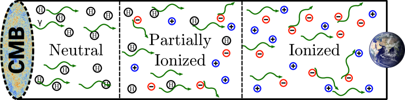
Figure 8: Photons from the CMB can be scattered by free electrons, called Thomson scattering, as they propagate to detectors on Earth. Only the total amount of Thomson scattering can be measured from the CMB, which is related to the timing of cosmic reionization.

While QSO absorption spectra probe the end of cosmic reionization, the CMB photons travel from the surface of last scattering to Earth and may scatter off free electrons, which is depicted schematically in Figure 8. Thomson scattering polarizes the CMB at large angular scales, resulting in a Thomson scattering optical depth $\tau_{\rm es}$ that is directly related to the column density of free electrons. This measure is an integrated one and tells us little about the reionization history and only about the approximate timing of reionization. A fully ionized IGM between $z=0$ and $z=6$ results in $\tau_{\rm es}=0.039$, and the remaining portion ($z>6$) of the integral depends on the reionization history $\bar{x}_{\rm e}(z)$. The most recent Planck 2018 [13] measurement of $\tau_{\rm es}=0.0561\pm 0.0071$, corresponding to a reionization redshift $z_{\rm re}=7.82\pm 0.71$ when the universe was half ionized ($\bar{x}_{\rm e}=0.5$).

4.4 Neutral hydrogen (21 cm) absorption and emission

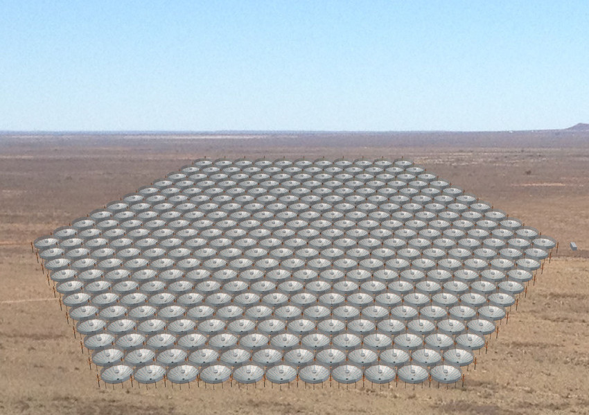
(a) Rendering of the final configuration of the Hydrogen Epoch of Reionization Array (HERA) with 331 antennas in South Africa.

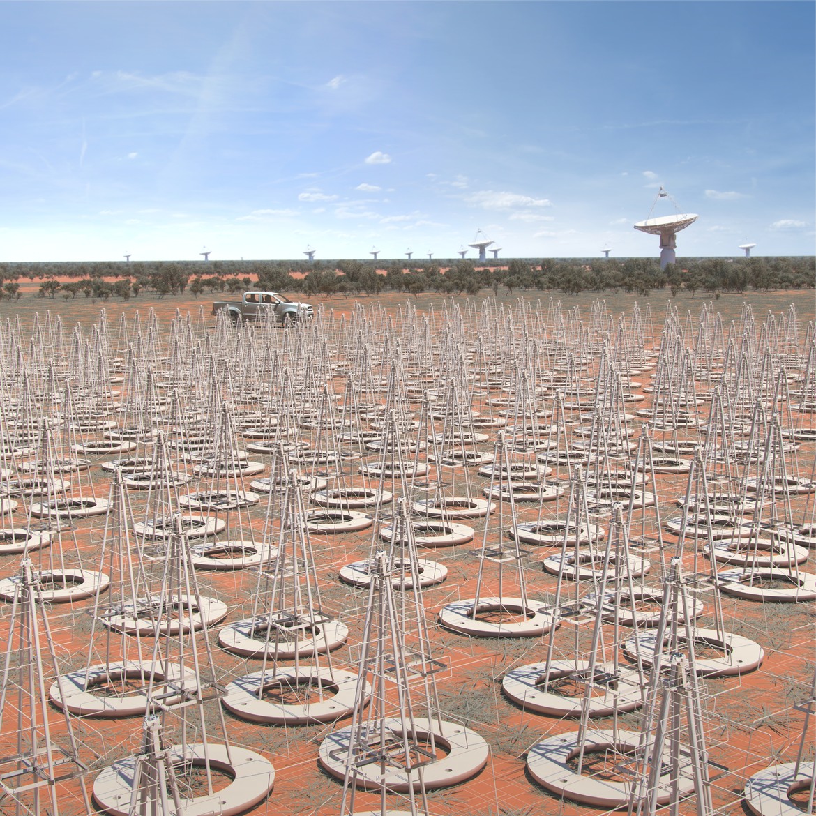
(b) Rendering of the Square Kilometer Array (SKA) to be co-located in Australia and South Africa.

Figure 9: Next generation 21-cm radio telescopes that will directly explore the Epoch of Reionization.

Perhaps the most direct measure of cosmic reionization comes from neutral hydrogen emission of the hyperfine splitting of the ground state, the 21-cm transition ($\nu=1420.4\;\textrm{MHz}$; $E_{21}=5.87\times 10^{-6}\;\textrm{eV}$). The hydrogen atom has a slightly lower energy when the spins of its proton and electron are anti-parallel than when they are parallel. The first detection of extraterrestrial 21-cm emission from neutral hydrogen happened in 1951 [64, 65], and it was not until four decades later that it was realized that 21-cm observations could be used to probe reionization [66].

When the IGM is mostly neutral, the universe is glowing in this radiation, and most of it is not absorbed as it travels toward Earth. Its detection is complicated by astrophysical foreground and terrestrial sources, especially considering that the redshifted 21-cm emission is at $101.5[(1+z)/14]^{-1}\;\textrm{MHz}$, squarely in the FM band. Before any stars form, the spin temperature

$$T_{\rm s}=T_{\ast}\ln\left(\frac{3n_{0}}{n_{1}}\right)$$ (10)

measures the relative occupancy of the electron spin levels. Here $T_{\ast}=E_{21}/k_{\rm B}=0.0682\;\textrm{K}$, and $n_{0}$ and $n_{1}$ are the singlet and triplet hyperfine levels of the ground state. The factor of 3 comes from the ratio of statistical weights between these levels. The spin temperature tightly couples to the CMB temperature $T_{\rm CMB}=2.73(1+z)\;\textrm{K}$ because the gas density is not high enough to couple with the kinetic temperature $T_{\rm K}$ that cools as $a^{-2}$ from adiabatic cosmic expansion.

Absorption or emission by neutral hydrogen changes the 21-cm (differential) brightness temperature $\delta T_{\rm b}$, which is the spin temperature relative to the background (CMB) temperature. Because the radiation is emanating from the neutral component of the IGM, it is usually multiplied by its neutral fraction $(1-\bar{x}_{\rm e})$. Positive and negative values denote emission and absorption at 21-cm. In addition to the neutral fraction of the IGM, X-ray and Ly$\alpha$ radiation can modify the 21-cm signal. Ly$\alpha$ radiation effects become dominate after $z\sim 30$ as the first stars begin to form, driving a decrease in $\delta T_{\rm b}$. Then the IGM begins to be partially ionized and heated by X-ray sources, increasing $\delta T_{\rm b}$. Eventually the IGM becomes ionized by UV sources, causing the brightness temperature $\delta T_{\rm b}$ to asymptote to zero as $\bar{x}_{\rm e}$ approaches unity. In summary, the 21-cm $\delta T_{\rm b}$ signal would appear a trough that deviates from zero and should smoothly vary because it is a volume average over the Universe.

A measurement of the brightness temperature evolution would place strong constraints on the reionization history and the nature of the ionizing sources. In particular, the location of the trough in $\delta T_{\rm b}$ relays information about the Ly$\alpha$ and X-ray emissivities of the first stars, black holes, and galaxies. Bowman et al. [67] reported on the first detection of such an absorption trough with the Experiment to Detect the Global Epoch of Reionization Signature (EDGES). It is centered at 78 MHz, corresponding to a redshift $z\sim 18$, and has anomalously sharp edges and a strong amplitude. First, its timing suggests that early star formation must have been intense in low-mass ($M_{\rm h}\lower 3.00003pt\hbox{$\,\buildrel>\over{\sim}\,$}10^{10}~{}{\textrm{M}_{\odot}}$) halos [68]. Second, its shape indicates a rapid coupling of the spin temperature to the gas temperature and was not predicted by prior models [69]. Kaurov et al. [70] argue that rare and massive galaxies at $z\sim 15-20$ are predominately responsible for this signal. Last, the absorption trough is consistent with a cold IGM prior to reionization. Perhaps the most mysterious aspect of the EDGES detection is its extreme depth, which suggests that the IGM is even colder than an adiabatically cooling IGM. This requires an additional cooling at very high redshifts ($z=30-100$) could indicate new physics, such as interactions between baryons and dark matter [71].

There are several experiments also aiming for the same detection, which include PAPER [72], LOFAR [73], MWA [74], HERA [75], and SKA [76]. It is essential to independently confirm this groundbreaking direct detection of reionization and to obtain additional observations of this cosmic phase transition.

4.5 Sources of reionization

From the direct and indirect IGM observations just discussed, we know that cosmic reionization occurred between $z=6-15$. But what sources were responsible for producing the required ionizing radiation for such a phase transition? QSOs are some of the brightest objects in the universe, but their number densities are not high enough [e.g. 77] to significantly contribute to the UVB and the overall photon budget of reionization. The latest studies have shown that they only contribute 1–5% of the photon budget at $z=6$ [e.g. 78, 79], however see Madau & Haardt [80] for a counterpoint. This leaves starlight from galaxies to propel reionization. Two important questions about the characteristics of high-redshift galaxies are: How abundant are galaxies as a function of luminosity and redshift? How many ionizing photons escaped from these galaxies into the IGM? The first question is addressed by counting galaxies and computing a luminosity function (LF), and the second is a harder quantity to measure as a neutral IGM is opaque to ionizing photons and needs to be inferred from their UV continuum redward of Ly$\alpha$.

Recent observational campaigns have provided valuable constraints on the nature of the first galaxies, their central BHs, and their role during reionization. In the rest-frame UV, the Hubble Space Telescope (HST) Ultra Deep Field [81] and Frontier Fields campaigns [82] can probe galaxies with stellar masses as small as $10^{7}~{}{\textrm{M}_{\odot}}$ at $z\lower 3.00003pt\hbox{$\,\buildrel>\over{\sim}\,$}6$ and as distant as $z\simeq 11$ [83, 84]. The LF is best described with a Schechter fit [85] as a function of luminosity,

$$\phi(L)=\phi^{*}\left(\frac{L}{L^{*}}\right)^{\alpha}\,\exp\left(-\frac{L}{L^{*}}\right)$$ (11)

that gives how many galaxies exist per comoving Mpc³ per decade of luminosity. As a function of absolute magnitude $M$, it reads as

$$\phi(M)=\frac{\ln(10)}{2.5}\phi^{*}10^{0.4(M-M^{*})(\alpha+1)}\exp\left[-10^{-0.4(M-M^{*})}\right].$$ (12)

The LF exponentially decays at the bright-end and is a power law at the faint-end. There are three parameters in this fit: the characteristic luminosity $L^{*}$ (or magnitude $M^{*}$) that denotes the transition between power-law and exponential decay, the number density normalization $\phi^{*}$, and faint-end slope $\alpha$. For the purposes of reionization sources, the faint-end is the most relevant because these faint galaxies should be very numerous. However the luminosity function should flatten and decrease at very low luminosities because galaxies cannot form in small halos (see Fig. 5). The faint-end slope and the luminosity at which the LF flattens is key when computing the total number density of galaxies and their ionizing emissivity. Various groups have constrained $\alpha\simeq-2$ at $z\geq 6$ [e.g. 86], and there are slight hints from the Frontier Fields that the LF flattens above a UV absolute magnitude of –14 [87, 88]. Based on this steep slope, there should be an unseen population of even fainter and more abundant galaxies that will eventually be detected by next-generation telescopes, such as JWST (James Webb Space Telescope) and 30-m class ground-based telescopes.

The ionizing emissivity ($\rho_{\rm UV}$; in units of erg s^-1 Hz^-1 Mpc^-3) is a key quantity in reionization calculations. Ionizing radiation is extremely difficult to observe, so we have to estimate it from the non-ionizing portion of galaxy spectra. Given a relation between total luminosity $L$ and star formation rate (SFR), we can integrate the product of SFR and the LF over luminosity to obtain a SFR density (in units of ${\textrm{M}_{\odot}}\;\textrm{yr}^{-1}\;\textrm{Mpc}^{-3}$). This quantity can then be converted into the ionizing emissivity $\rho_{\rm UV}$ with two factors. The first is the number of ionizing photons emitted per stellar baryon $f_{\gamma}\simeq 4000-13000$, which depends on stellar metallicity. The second and most uncertain is the fraction $f_{\rm esc}$ of ionizing photons that escape into IGM. Finkelstein et al. [89] used Ly$\alpha$ forest observations to place an upper limit on the average $\langle f_{\rm esc}\rangle<0.13$ at $z=6$. However this does not prevent the average $f_{\rm esc}$ from being larger at higher redshifts [45]. Direct measurements of $f_{\rm esc}$ is impossible during EoR because the IGM optical depth in the Ly$\alpha$ forest only drops to unity at $z\sim 3$ as these absorption systems become less abundant with time. Nevertheless, deep narrow-band galaxy spectroscopy and imaging have detected Lyman continuum emission in numerous $z\sim 3$ galaxies with $f_{\rm esc}$ values ranging from an upper limit of 7%–9% for bright galaxies [90] to 10%–30% for fainter Ly$\alpha$ emitters [91] and $33\pm 7\%$ for ’Lyman-continuum galaxies’ [92]. These measurements combined with theoretical calculations may be taken as a guide to the $f_{\rm esc}$ values expected from EoR galaxies.

4.6 Summary of observations

Having reviewed the primary observational constraints on cosmic reionization, there are clearly several independent measures of this grand event. The end of reionization is probed by QSO absorption spectra. The Ly$\alpha$ forest and GP troughs are used to constrain the residual neutral fraction ($\simeq 10^{-4}$ at $z=6$) and remaining neutral patches. The thermal state of the Ly$\alpha$ forest retains some ’fossil memory’ of its initial heating during reionization and can be used to constraint the timing and heating source spectrum. Furthermore, the evolution of the UVB is determined from the Ly$\alpha$ forest and is steeply increasing with time at $z>5$. The CMB provides both an integral measure of reionization with the universe being half-ionized at $z_{\rm re}=7.82\pm 0.71$. Future 21-cm experiments will be able to further constrain the reionization history and the nature of the ionizing sources. From the measurement of the steep faint-end LF slope $\alpha\simeq-2$ at $z\geq 6$, young star-forming galaxies are most likely the primary drivers of reionization.

5 Reionization Modeling

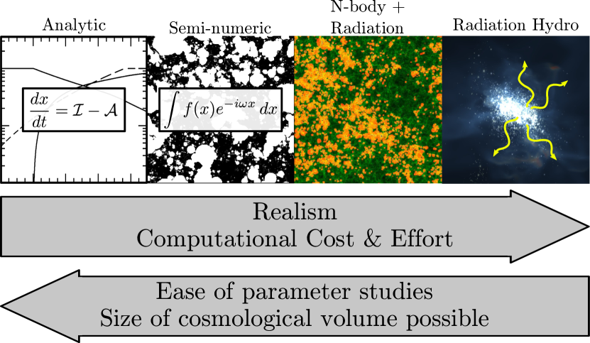
Figure 10: Four different numerical models that capture the process of cosmic reionization: volume-averaged analytic models; spatially-dependent semi-numeric models; radiative transfer calculations that use matter distributions from N-body calculations; full radiation hydrodynamic galaxy formation simulations. The increased physicality and realism comes at the price of added computational cost, limiting the ability to explore different reionization models and the associated parameter space.

Cosmic reionization can be modeled in a variety of methods, which are depicted in Figure 10. They range from a volume-averaged approach, taking less than a second to compute, to full radiation hydrodynamics cosmological simulations of galaxies and the IGM, taking months to complete. These methods have their advantages and disadvantages, and they complement each other. They use the appropriate observational constraints to make predictions about the reionization history, the nature of its sources, and future observational techniques on further constraining this epoch.

5.1 Volume-averaged analytical models

On the most basic level, reionization models count the number of ionizing photons and compare it with the number of hydrogen atoms in some specified volume, which was first (to the best of the author’s knowledge) studied by Arons & McCray [93] in a time-dependent approach. As we have covered in the basic physics of ionization balance, recombinations can still occur in a strong ionizing radiation field, and thus cosmic reionization requires more than one ionizing photon per hydrogen atom. The rate of change in the ionized fraction $x_{\rm e}$ of the universe can be computed by considering the comoving photon emissivity $\dot{n}_{\gamma}$ and recombinations in the ionized regions,

$$\frac{dx_{\rm e}}{dt}=\frac{\dot{n}_{\gamma}}{\bar{n}_{\rm H}}-\frac{x_{\rm e}}{\bar{t}_{\rm rec}},$$ (13)

This differential equation is integrated from a neutral medium ($x_{\rm e}=0$) at very early times before any UV sources form ($z\sim 50-100$) until the universe is completely ionized ($x_{\rm e}=1$). Its evolution gives a reionization history, which then can be integrated to obtain the Thomson scattering optical depth $\tau_{\rm es}$.

Here $\bar{n}_{\rm H}$ is the mean comoving hydrogen number density, and $\bar{t}_{\rm rec}=[C\alpha_{\rm B}\bar{n}_{\rm H}(1+Y/4X)(1+z)^{3}]^{-1}$ is an effective recombination time. Recall that $X=0.76$ and $Y=1-X$ are the hydrogen and helium number fractions, respectively. The clumping factor $C\approx 3-5$ during EoR accounts for enhanced recombinations in a clumpy ionized IGM [e.g. 94, 95]. There are various definitions for the clumping factor [see 96, for a discussion], but the most straightforward definition is $C\equiv\langle\rho^{2}\rangle/\langle\rho\rangle^{2}$ and is restricted to ionized regions.

To calculate the number density of ionizing photons $\dot{n}_{\gamma}$ that escape into the IGM, we first must calculate the fraction $f_{\rm c}$ of matter that has collapsed into DM halos and then luminous objects. Most of the uncertainties in reionization modeling originates from the halo-galaxy connection. More specifically, given a DM halo, the following main ingredients are needed to calculate the ionizing emissivity: (i) the star formation rate or stellar mass, (ii) the stellar ionizing efficiency (i.e. number of ionizing photons per stellar baryon), and (iii) the UV escape fraction $f_{\rm esc}$. For a time and halo mass independent model [e.g. 97, 98], $\dot{n}_{\gamma}=f_{\rm esc}f_{\gamma}\bar{\rho}_{\star}$, where $\bar{\rho}_{\star}$ is the star formation rate density and recall that $f_{\gamma}$ is the photon to stellar baryon ratio. However, simulations have shown that star formation rates and $f_{\rm esc}$ values are strong functions of halo mass $M_{\rm vir}$. A more accurate value for the ionizing emissivity can be calculated by integrating over all halo masses,

$$\dot{n}_{\gamma}=\int_{M_{\rm min}}^{\infty}f_{\rm esc}f_{\gamma}(f_{\rm gas}f_{\star}\dot{f}_{\rm c}M_{\rm vir})dM_{\rm vir},$$ (14)

where all of the factors are functions of halo mass, and the product inside the parentheses is the star formation rate density in halo masses between $M$ and $M+dM$. Here $M_{\rm min}$ is the minimum halo mass that hosts star formation; $f_{\rm gas}\equiv M_{\rm gas}/M_{\rm vir}$ is the gas fraction in a halo; $f_{\star}\equiv M_{\star}/M_{\rm gas}$ is the star formation efficiency from this gas, and $\dot{f}_{\rm c}$ is the time derivative of the collapsed mass fraction in halos. This integral can be solved numerically if given functional forms (either smooth or piecewise [e.g. 99, 44]), which are usually computed from simulations [e.g. 100] or semi-analytic models [e.g. 101] of early galaxy formation.

5.2 Semi-numeric models

The latest observational constraints strongly suggest that reionization is driven by galaxies and their UV radiation, and thus it is a relatively local process. Semi-numeric models originated from an analytical (excursion set) treatment of reionization [102] that made the fundamental assumption that overdense regions drive reionization. With this assumption, one asserts that if the number of ionizing photons, corrected for recombinations, exceeds the number of baryons in some region, then the region must be ionized. This model has been extended to three-dimensional volumes [e.g. 103, 104, 99] and can accurately generate full density, velocity, and ionization fields without the need to follow the underlying physics.

From a single set of cosmological initial conditions, usually given in a 3-D lattice with $N_{\rm cell}^{3}$ computational cells, at high redshift $z\sim 100$, semi-numeric models can compute the ionized fraction for each cell. One major advantage to this method is that these models can calculate $x_{\rm e}(\mathbf{r})$ at any redshift without performing a time-dependent integral. Namely, a cell is considered to be ionized when

$$f_{\rm c}(\mathrm{r},M_{\rm min},R,z)\geq\zeta^{-1},$$ (15)

where $\zeta$ is the ionization efficiency, and $f_{\rm c}$ is the collapsed mass fraction inside a sphere of radius $R$ in halos with masses $M>M_{\rm min}$. This value of $R$ is iterated from a large length, usually the UV photon mean free path, down to the width of a single cell. The ionization efficiency can be parameterized [e.g. 56], not unlike analytical models, to be dependent on the galaxy properties. This method can fully determine the ionization state at any time and position in the volume. The most computationally intensive portion of semi-numeric calculations involves Fast Fourier Transforms (FFTs) and usually takes on the order of core-hours for a single $2048^{3}$ realization, including the initial condition generation.

5.3 Cosmological radiative transfer simulations

Cosmological $N$-body simulations evolve the cosmic density field and associated halos, which are then used to calculate the evolution of time- and space-dependent ionization fields. They assume that gas follows the DM, which is a good assumption on large-scales and in larger halos ($M\lower 3.00003pt\hbox{$\,\buildrel>\over{\sim}\,$}10^{9}{\textrm{M}_{\odot}}$), and then populate these halos with galaxies that produce ionizing radiation. It is transported through the IGM, usually with ray tracing methods that solve the cosmological radiative transfer equation, which in comoving coordinates [105] is

$$\frac{1}{c}\;\frac{\partial I_{\nu}}{\partial t}+\frac{\hat{\mathbf{n}}\cdot\nabla I_{\nu}}{\bar{a}}-\frac{H}{c}\;\left(\nu\frac{\partial I_{\nu}}{\partial\nu}-3I_{\nu}\right)=-\kappa_{\nu}I_{\nu}+j_{\nu},$$ (16)

reproducing inhomogeneous reionization. Here $I_{\nu}\equiv I(\nu,\mathbf{x},\Omega,t)$ is the radiation specific intensity in units of energy per time $t$ per solid angle per unit area per frequency $\nu$. $H=\dot{a}/a$ is the Hubble parameter. $\bar{a}=a/a_{em}$ is the ratio of scale factors at the current time and time of emission. The second term represents the propagation of radiation, where the factor $1/\bar{a}$ accounts for cosmic expansion. The third term describes both the cosmological redshift and dilution of radiation. On the right hand side, the first term considers the absorption coefficient $\kappa_{\nu}\equiv\kappa_{\nu}(\mathbf{x},\nu,t)$. The second term $j_{\nu}\equiv j_{\nu}(\mathbf{x},\nu,t)$ is the emission coefficient that includes any point sources of radiation or diffuse radiation.

Solving this equation is difficult because of its high dimensionality; however, we can make some appropriate approximations to reduce its complexity in order to include radiation transport in numerical calculations. Typically timesteps in dynamic calculations are small enough so that $\Delta a/a\ll 1$, therefore $\bar{a}=1$ in any given timestep, reducing the second term to $\hat{\mathbf{n}}\partial I_{\nu}/\partial\mathbf{x}$. To determine the importance of the third term, we evaluate the ratio of the third term to the second term. This is $HL/c$, where $L$ is the simulation box length. If this ratio is $\ll 1$, we can ignore the third term. For example at $z=5$, this ratio is 0.1 when $L=c/H(z=5)$ = 53 proper Mpc. In large boxes where the light crossing time is comparable to the Hubble time, then it becomes important to consider cosmological redshifting and dilution of the radiation. Thus equation (16) reduces to the non-cosmological form in this local approximation,

$$\frac{1}{c}\frac{\partial I_{\nu}}{\partial t}+\hat{\mathbf{n}}\frac{\partial I_{\nu}}{\partial\mathbf{x}}=-\kappa_{\nu}I_{\nu}+j_{\nu}.$$ (17)

Ray tracing methods represent the source term $j_{\nu}$ as point sources of radiation (e.g. stars, galaxies, quasars) that emit radial rays that are propagated along the direction $\hat{\mathbf{n}}$.

The downside to this method is that it neglects any hydrodynamics and must make assumptions about the ionizing luminosity escaping from the halos, the IGM clumping factor $C$, and the suppression of star formation in low-mass ($M\lower 3.00003pt\hbox{$\,\buildrel<\over{\sim}\,$}10^{9}{\textrm{M}_{\odot}}$) halos. Such calculations are performed in either (i) post-processing with the radiative transfer calculated on density field and halo catalog written to disk, or (ii) inline where the halo catalogs and radiation sources are computed on-the-fly, and radiation is traced through the density field that is stored in memory. The largest simulations to-date have over 100 billion particles and simulate domains of over 500 comoving Mpc on a side, and such simulations consume a couple of million core-hours [e.g. 106]. They produce similar results as semi-numeric models but with a larger dynamic range, with higher resolution in collapsed regions, thus can follow the small-scale ionization fluctuations to greater accuracy.

5.4 Full radiation hydrodynamics simulations

Perhaps the most accurate and computationally expensive calculations are full radiation hydrodynamics simulations of cosmological galaxy formation and reionization. Only in the past decade or so, computational resources have become large enough, along with algorithmic advances, to cope with the requirements of such calculations. There are two popular methods to solve the radiative transfer equation coupled to hydrodynamics in three dimensions:

• Moment methods: The angular moments of the radiation field describe its angular structure, which are related to energy, flux, and radiation pressure [107]. These have been implemented in conjunction with short characteristics [108], with long characteristics [109], with a variable Eddington tensor in the optically-thin limit [110] and the general case [111], and with an M1 closure relation [112, 113]. Moment methods have the advantage of being efficient and independent of the number of radiation sources. However, they are diffusive and result in incorrect shadows in some situations.

• Ray tracing: Radiation can be propagated along rays that extend through a computational grid [e.g. 114, 115, 116] or particle set [e.g. 117, 118, 119], as discussed previously. In general, these methods are very accurate but computationally expensive because the radiation field must be well sampled by the rays with respect to the spatial resolution of the domain.

In addition to following the DM dynamics, like in the radiative transfer simulations, they follow the hydrodynamics of the cosmological domain that allows for the treatment of gaseous collapses within halos that are driven by radiative cooling. These radiative processes are computed through a non-equilibrium chemical network [e.g. 120]. However computational run-time and memory limits the resolution of these simulations, which are typically $\sim 10$ times more expensive than the cosmological radiative transfer simulations. Depending on the domain size and resolution, ’sub-grid’ star formation prescriptions spawn particles that represent either entire galaxies or individual stellar clusters. Based on this prescription, the particle has an ionizing luminosity, whose radiation is the source of the radiative transfer equation (Equation 16 or 17). Because the radiation transport is coupled with the hydrodynamics, this equation must be solved with either small timesteps and/or the appropriate approximations [116]. Thus, the radiation sources and the ensuing hydrodynamic response can be modeled without relying on a halo-galaxy relationship. The suppression of star formation, especially in low-mass galaxies can be directly modeled, along with the regulation of star formation that results in a more accurate description of the ionizing sources during the EoR and the process of reionization itself. That being said, there still exists uncertainties, arising from the sub-grid models and convergence issues of the numerical solvers with respect to resolution.

6 Conclusions

Cosmic reionization is the last cosmological phase transition. There is strong observational evidence that it ended nearly one billion years after the Big Bang. The first generations of galaxies primarily powered this grand event in the cosmic timeline. Because structure forms hierarchically, these first galaxies are the building blocks of all galaxies we see today, and their properties are passed along as galaxies assemble. Thus, further constraints from the epoch of reionization will play a key role in solidifying theories of galaxy formation and cosmology.

However there still are unanswered questions in its exact timing, its progression, its nature, and the role of the first galaxies played during the epoch of reionization. These questions will be elucidated with the upcoming James Webb Space Telescope, ground-based 30-m class telescopes, and more accurate CMB and 21-cm experiments, all set to be commissioned within the next decade. Observing both the reionizing universe and the galaxies responsible for this transition is paramount in augmenting our knowledge of this formative period in the universe.

Notes on contributor

John Wise is the Dunn Family Associate Professor in the School of Physics and Center for Relativistic Astrophysics at the Georgia Institute of Technology. He uses numerical simulations to study the formation and evolution of galaxies and their black holes. He is one of the lead developers of the community-driven, open-source astrophysics code Enzo (enzo-project.org). He received his B.S. in Physics from the Georgia Tech in 2001. He then studied at Stanford University, where he received his Ph.D. in Physics in 2007. He went on to work at NASA’s Goddard Space Flight Center as a NASA Postdoctoral Fellow. Then in 2009, he was awarded the Hubble Fellowship which he took to Princeton University before arriving at Georgia Tech in 2011, coming back home after ten years roaming the nation.

References

- [1] Minkowski R. A New Distant Cluster of Galaxies. ApJ. 1960 Nov;132:908–910.
- [2] Matthews TA, Bolton JG, Greenstein JL, et al. paper presented at the 107th meeting of the AAS. In: American Astronomical Society Meeting Abstracts; Vol. 107; Dec.; 1960.
- [3] Schmidt M. 3C 273 : A Star-Like Object with Large Red-Shift. Nature. 1963 Mar;197:1040.
- [4] Hoyle F, Fowler WA. On the nature of strong radio sources. MNRAS. 1963;125:169.
- [5] Schmidt M, Matthews TA. Redshift of the Quasi-Stellar Radio Sources 3c 47 and 3c 147. ApJ. 1964 Feb;139:781.
- [6] Sandage A. The Existence of a Major New Constituent of the Universe: the Quasistellar Galaxies. ApJ. 1965 May;141:1560.
- [7] Osterbrock DE, Parker RAR. Excitation of the Optical Emission Lines in Quasi-Stellar Radio Sources. ApJ. 1966 Jan;143:268.
- [8] Salpeter EE. Accretion of Interstellar Matter by Massive Objects. ApJ. 1964 Aug;140:796–800.
- [9] Zel’dovich YB. The Fate of a Star and the Evolution of Gravitational Energy Upon Accretion. Soviet Physics Doklady. 1964 Sep;9:195.
- [10] Lynden-Bell D. Galactic Nuclei as Collapsed Old Quasars. Nature. 1969 Aug;223:690–694.
- [11] Tananbaum H, Avni Y, Branduardi G, et al. X-ray studies of quasars with the Einstein Observatory. ApJ. 1979 Nov;234:L9–L13.
- [12] Gunn JE, Peterson BA. On the Density of Neutral Hydrogen in Intergalactic Space. ApJ. 1965 Nov;142:1633–1641.
- [13] Planck Collaboration, Aghanim N, Akrami Y, et al. Planck 2018 results. VI. Cosmological parameters. arXiv e-prints. 2018 Jul;:arXiv:1807.06209.
- [14] Rees MJ. The Universe at z 5: When and How Did the ’Dark Age’ End? In: N R Tanvir, A Aragon-Salamanca, & J V Wall, editor. The Hubble Space Telescope and the High Redshift Universe; 1997. p. 115–+.
- [15] Skillman SW, Warren MS, Turk MJ, et al. Dark Sky Simulations: Early Data Release. ArXiv e-prints (14072600). 2014 Jul;.
- [16] Peebles PJE. Large-scale background temperature and mass fluctuations due to scale-invariant primeval perturbations. ApJ. 1982 Dec;263:L1–L5.
- [17] Blumenthal GR, Faber SM, Primack JR, et al. Formation of galaxies and large-scale structure with cold dark matter. Nature. 1984 Oct;311:517–525.
- [18] Davis M, Efstathiou G, Frenk CS, et al. The evolution of large-scale structure in a universe dominated by cold dark matter. ApJ. 1985 May;292:371–394.
- [19] Lynden-Bell D. Statistical mechanics of violent relaxation in stellar systems. MNRAS. 1967;136:101–+.
- [20] Gunn JE, Gott JR III. On the Infall of Matter Into Clusters of Galaxies and Some Effects on Their Evolution. ApJ. 1972 Aug;176:1.
- [21] Strömgren B. The Physical State of Interstellar Hydrogen. ApJ. 1939 May;89:526–+.
- [22] Davé R, Cen R, Ostriker JP, et al. Baryons in the Warm-Hot Intergalactic Medium. ApJ. 2001 May;552:473–483.
- [23] Haardt F, Madau P. Radiative Transfer in a Clumpy Universe. IV. New Synthesis Models of the Cosmic UV/X-Ray Background. ApJ. 2012 Feb;746:125.
- [24] Gnedin NY. Effect of Reionization on Structure Formation in the Universe. ApJ. 2000 Oct;542:535–541.
- [25] Meiksin A, Madau P. On the photoionization of the intergalactic medium by quasars at high redshift. ApJ. 1993 Jul;412:34–55.
- [26] Tseliakhovich D, Hirata C. Relative velocity of dark matter and baryonic fluids and the formation of the first structures. Phys. Rev. D. 2010 Oct;82(8):083520.
- [27] Peebles PJE. Principles of Physical Cosmology. ; 1993.
- [28] Barkana R, Loeb A. In the beginning: the first sources of light and the reionization of the universe. Phys. Rep.. 2001 Jul;349:125–238.
- [29] Asplund M, Grevesse N, Sauval AJ, et al. The Chemical Composition of the Sun. Annual Review of Astronomy and Astrophysics. 2009 Sep;47(1):481–522.
- [30] Bromm V, Ferrara A, Coppi PS, et al. The fragmentation of pre-enriched primordial objects. MNRAS. 2001 Dec;328:969–976.
- [31] Abel T, Bryan GL, Norman ML. The Formation of the First Star in the Universe. Science. 2002 Jan;295:93–98.
- [32] Machacek ME, Bryan GL, Abel T. Simulations of Pregalactic Structure Formation with Radiative Feedback. ApJ. 2001 Feb;548:509–521.
- [33] O’Leary RM, McQuinn M. The Formation of the First Cosmic Structures and the Physics of the z ~ 20 Universe. ApJ. 2012 Nov;760:4.
- [34] Schauer ATP, Glover SCO, Klessen RS, et al. The influence of streaming velocities on the formation of the first stars. MNRAS. 2019 Apr;484(3):3510–3521.
- [35] Wise JH, Turk MJ, Norman ML, et al. The Birth of a Galaxy: Primordial Metal Enrichment and Stellar Populations. ApJ. 2012 Jan;745:50.
- [36] Hirano S, Hosokawa T, Yoshida N, et al. Primordial star formation under the influence of far ultraviolet radiation: 1540 cosmological haloes and the stellar mass distribution. MNRAS. 2015 Mar;448:568–587.
- [37] Turk MJ, Abel T, O’Shea B. The Formation of Population III Binaries from Cosmological Initial Conditions. Science. 2009 Jul;325:601–.
- [38] Greif TH, Bromm V, Clark PC, et al. Formation and evolution of primordial protostellar systems. MNRAS. 2012 Jul;424:399–415.
- [39] Schaerer D. On the properties of massive Population III stars and metal-free stellar populations. A&A. 2002 Jan;382:28–42.
- [40] Alvarez MA, Bromm V, Shapiro PR. The H II Region of the First Star. ApJ. 2006 Mar;639:621–632.
- [41] Kimm T, Cen R. Escape Fraction of Ionizing Photons during Reionization: Effects due to Supernova Feedback and Runaway OB Stars. ApJ. 2014 Jun;788:121.
- [42] Kimm T, Katz H, Haehnelt M, et al. Feedback-regulated star formation and escape of LyC photons from mini-haloes during reionization. MNRAS. 2017 Apr;466(4):4826–4846.
- [43] Xu H, Wise JH, Norman ML, et al. Galaxy Properties and UV Escape Fractions during the Epoch of Reionization: Results from the Renaissance Simulations. ApJ. 2016 Dec;833:84.
- [44] Wise JH, Demchenko VG, Halicek MT, et al. The birth of a galaxy - III. Propelling reionization with the faintest galaxies. MNRAS. 2014 Aug;442:2560–2579.
- [45] Robertson BE, Furlanetto SR, Schneider E, et al. New Constraints on Cosmic Reionization from the 2012 Hubble Ultra Deep Field Campaign. ApJ. 2013 May;768:71.
- [46] Ma X, Kasen D, Hopkins PF, et al. The difficulty of getting high escape fractions of ionizing photons from high-redshift galaxies: a view from the FIRE cosmological simulations. MNRAS. 2015 Oct;453:960–975.
- [47] Xu H, Ahn K, Wise JH, et al. Heating the Intergalactic Medium by X-Rays from Population III Binaries in High-redshift Galaxies. ApJ. 2014 Aug;791:110.
- [48] Mesinger A, Ferrara A, Spiegel DS. Signatures of X-rays in the early Universe. MNRAS. 2013 May;431:621–637.
- [49] Bañados E, Venemans BP, Mazzucchelli C, et al. An 800-million-solar-mass black hole in a significantly neutral Universe at a redshift of 7.5. Nature. 2018 Jan;553:473–476.
- [50] Fan X, Strauss MA, Becker RH, et al. Constraining the Evolution of the Ionizing Background and the Epoch of Reionization with z~6 Quasars. II. A Sample of 19 Quasars. AJ. 2006 Jul;132:117–136.
- [51] Alvarez MA, Wise JH, Abel T. Accretion onto the First Stellar-Mass Black Holes. ApJ. 2009 Aug;701:L133–L137.
- [52] Greig B, Mesinger A, Haiman Z, et al. Are we witnessing the epoch of reionisation at z = 7.1 from the spectrum of J1120+0641? MNRAS. 2017 Apr;466(4):4239–4249.
- [53] Becker GD, Bolton JS, Madau P, et al. Evidence of patchy hydrogen reionization from an extreme Ly trough below redshift six. MNRAS. 2015 Mar;447:3402–3419.
- [54] Songaila A. The Evolution of the Intergalactic Medium Transmission to Redshift 6. AJ. 2004 May;127:2598–2603.
- [55] Mesinger A. Was reionization complete by z ~ 5-6? MNRAS. 2010 Sep;407:1328–1337.
- [56] Greig B, Mesinger A. The global history of reionization. MNRAS. 2017 Mar;465(4):4838–4852.
- [57] McDonald P, Miralda-Escudé J, Rauch M, et al. A Measurement of the Temperature-Density Relation in the Intergalactic Medium Using a New Ly Absorption-Line Fitting Method. ApJ. 2001 Nov;562:52–75.
- [58] York DG, Adelman J, Anderson JE Jr, et al. The Sloan Digital Sky Survey: Technical Summary. AJ. 2000 Sep;120:1579–1587.
- [59] Becker GD, Bolton JS. New measurements of the ionizing ultraviolet background over 2 z 5 and implications for hydrogen reionization. MNRAS. 2013 Dec;436:1023–1039.
- [60] Schaye J, Theuns T, Rauch M, et al. The thermal history of the intergalactic medium∗. MNRAS. 2000 Nov;318:817–826.
- [61] Hui L, Gnedin NY. Equation of state of the photoionized intergalactic medium. MNRAS. 1997 Nov;292:27.
- [62] Bolton JS, Becker GD, Wyithe JSB, et al. A first direct measurement of the intergalactic medium temperature around a quasar at z = 6. MNRAS. 2010 Jul;406:612–625.
- [63] Bolton JS, Becker GD, Raskutti S, et al. Improved measurements of the intergalactic medium temperature around quasars: possible evidence for the initial stages of He II reionization at z 6. MNRAS. 2012 Feb;419:2880–2892.
- [64] Ewen HI, Purcell EM. Observation of a Line in the Galactic Radio Spectrum: Radiation from Galactic Hydrogen at 1,420 Mc./sec. Nature. 1951 Sep;168:356.
- [65] Muller CA, Oort JH. Observation of a Line in the Galactic Radio Spectrum: The Interstellar Hydrogen Line at 1,420 Mc./sec., and an Estimate of Galactic Rotation. Nature. 1951 Sep;168:357–358.
- [66] Scott D, Rees MJ. The 21-cm line at high redshift: a diagnostic for the origin of large scale structure. MNRAS. 1990 Dec;247:510.
- [67] Bowman JD, Rogers AEE, Monsalve RA, et al. An absorption profile centred at 78 megahertz in the sky-averaged spectrum. Nature. 2018 Mar;555(7694):67–70.
- [68] Mirocha J, Furlanetto SR. What does the first highly redshifted 21-cm detection tell us about early galaxies? MNRAS. 2019 Feb;483(2):1980–1992.
- [69] Cohen A, Fialkov A, Barkana R, et al. Charting the parameter space of the global 21-cm signal. MNRAS. 2017 Dec;472(2):1915–1931.
- [70] Kaurov AA, Venumadhav T, Dai L, et al. Implication of the Shape of the EDGES Signal for the 21 cm Power Spectrum. ApJ. 2018 Sep;864(1):L15.
- [71] Barkana R. Possible interaction between baryons and dark-matter particles revealed by the first stars. Nature. 2018 Mar;555(7694):71–74.
- [72] Parsons AR, Backer DC, Foster GS, et al. The Precision Array for Probing the Epoch of Re-ionization: Eight Station Results. AJ. 2010 Apr;139:1468–1480.
- [73] van Haarlem MP, Wise MW, Gunst AW, et al. LOFAR: The LOw-Frequency ARray. A&A. 2013 Aug;556:A2.
- [74] Bowman JD, Cairns I, Kaplan DL, et al. Science with the Murchison Widefield Array. PASA. 2013 Apr;30:e031.
- [75] Neben AR, Bradley RF, Hewitt JN, et al. The Hydrogen Epoch of Reionization Array Dish. I. Beam Pattern Measurements and Science Implications. ApJ. 2016 Aug;826:199.
- [76] Dewdney PE, Hall PJ, Schilizzi RT, et al. The square kilometre array. Proceedings of the IEEE. 2009;97(8):1482–1496.
- [77] Kashikawa N, Ishizaki Y, Willott CJ, et al. The Subaru High-z Quasar Survey: Discovery of Faint z ~ 6 Quasars. ApJ. 2015 Jan;798:28.
- [78] Willott CJ, Albert L, Arzoumanian D, et al. Eddington-limited Accretion and the Black Hole Mass Function at Redshift 6. AJ. 2010 Aug;140:546–560.
- [79] Grissom RL, Ballantyne DR, Wise JH. On the contribution of active galactic nuclei to reionization. A&A. 2014 Jan;561:A90.
- [80] Madau P, Haardt F. Cosmic Reionization after Planck: Could Quasars Do It All? ApJ. 2015 Nov;813:L8.
- [81] Ellis RS, McLure RJ, Dunlop JS, et al. The Abundance of Star-forming Galaxies in the Redshift Range 8.5-12: New Results from the 2012 Hubble Ultra Deep Field Campaign. ApJ. 2013 Jan;763:L7.
- [82] Coe D, Bradley L, Zitrin A. Frontier Fields: High-redshift Predictions and Early Results. ApJ. 2015 Feb;800:84.
- [83] Laporte N, Infante L, Troncoso Iribarren P, et al. Young Galaxy Candidates in the Hubble Frontier Fields. III. MACS J0717.5+3745. ApJ. 2016 Apr;820:98.
- [84] Oesch PA, Brammer G, van Dokkum PG, et al. A Remarkably Luminous Galaxy at z=11.1 Measured with Hubble Space Telescope Grism Spectroscopy. ApJ. 2016 Mar;819:129.
- [85] Schechter P. An analytic expression for the luminosity function for galaxies. ApJ. 1976 Jan;203:297–306.
- [86] McLure RJ, Dunlop JS, Bowler RAA, et al. A new multifield determination of the galaxy luminosity function at z = 7-9 incorporating the 2012 Hubble Ultra-Deep Field imaging. MNRAS. 2013 Jul;432:2696–2716.
- [87] Livermore RC, Finkelstein SL, Lotz JM. Directly Observing the Galaxies Likely Responsible for Reionization. ApJ. 2017 Feb;835(2):113.
- [88] Bouwens RJ, Oesch PA, Illingworth GD, et al. The z ̵̃ 6 Luminosity Function Fainter than -15 mag from the Hubble Frontier Fields: The Impact of Magnification Uncertainties. ApJ. 2017 Jul;843(2):129.
- [89] Finkelstein SL, Papovich C, Ryan RE, et al. CANDELS: The Contribution of the Observed Galaxy Population to Cosmic Reionization. ApJ. 2012 Oct;758:93.
- [90] Siana B, Shapley AE, Kulas KR, et al. A Deep Hubble Space Telescope and Keck Search for Definitive Identification of Lyman Continuum Emitters at z~3.1. ApJ. 2015 May;804:17.
- [91] Nestor DB, Shapley AE, Kornei KA, et al. A Refined Estimate of the Ionizing Emissivity from Galaxies at z ~= 3: Spectroscopic Follow-up in the SSA22a Field. ApJ. 2013 Mar;765:47.
- [92] Cooke J, Ryan-Weber EV, Garel T, et al. Lyman-continuum galaxies and the escape fraction of Lyman-break galaxies. MNRAS. 2014 Jun;441:837–851.
- [93] Arons J, McCray R. Photo-Ionization of Intergalactic Hydrogen by Quasars. Astrophys. Lett.. 1970;5:123.
- [94] Pawlik AH, Schaye J, van Scherpenzeel E. Keeping the Universe ionized: photoheating and the clumping factor of the high-redshift intergalactic medium. MNRAS. 2009 Apr;394:1812–1824.
- [95] So GC, Norman ML, Reynolds DR, et al. Fully Coupled Simulation of Cosmic Reionization. II. Recombinations, Clumping Factors, and the Photon Budget for Reionization. ApJ. 2014 Jul;789:149.
- [96] Finlator K, Oh SP, Özel F, et al. Gas clumping in self-consistent reionization models. MNRAS. 2012 Dec;427:2464–2479.
- [97] Madau P, Haardt F, Rees MJ. Radiative Transfer in a Clumpy Universe. III. The Nature of Cosmological Ionizing Sources. ApJ. 1999 Apr;514:648–659.
- [98] Robertson BE, Ellis RS, Furlanetto SR, et al. Cosmic Reionization and Early Star-forming Galaxies: A Joint Analysis of New Constraints from Planck and the Hubble Space Telescope. ApJ. 2015 Apr;802:L19.
- [99] Alvarez MA, Finlator K, Trenti M. Constraints on the Ionizing Efficiency of the First Galaxies. ApJ. 2012 Nov;759:L38.
- [100] Chen P, Wise JH, Norman ML, et al. Scaling Relations for Galaxies Prior to Reionization. ApJ. 2014 Nov;795:144.
- [101] Benson AJ, Sugiyama N, Nusser A, et al. The epoch of reionization. MNRAS. 2006 Jul;369:1055–1080.
- [102] Furlanetto SR, Zaldarriaga M, Hernquist L. The Growth of H II Regions During Reionization. ApJ. 2004 Sep;613:1–15.
- [103] Zahn O, Lidz A, McQuinn M, et al. Simulations and Analytic Calculations of Bubble Growth during Hydrogen Reionization. ApJ. 2007 Jan;654:12–26.
- [104] Mesinger A, Furlanetto S. Efficient Simulations of Early Structure Formation and Reionization. ApJ. 2007 Nov;669:663–675.
- [105] Gnedin NY, Ostriker JP. Reionization of the Universe and the Early Production of Metals. ApJ. 1997 Sep;486:581–+.
- [106] Iliev IT, Mellema G, Ahn K, et al. Simulating cosmic reionization: how large a volume is large enough? MNRAS. 2014 Mar;439:725–743.
- [107] Auer LH, Mihalas D. On the use of variable Eddington factors in non-LTE stellar atmospheres computations. MNRAS. 1970;149:65–+.
- [108] Davis SW, Stone JM, Jiang YF. A Radiation Transfer Solver for Athena Using Short Characteristics. ApJS. 2012 Mar;199:9.
- [109] Finlator K, Özel F, Davé R. A new moment method for continuum radiative transfer in cosmological re-ionization. MNRAS. 2009 Mar;393:1090–1106.
- [110] Gnedin NY, Abel T. Multi-dimensional cosmological radiative transfer with a Variable Eddington Tensor formalism. New A. 2001 Oct;6:437–455.
- [111] Jiang YF, Stone JM, Davis SW. An Algorithm for Radiation Magnetohydrodynamics Based on Solving the Time-dependent Transfer Equation. ApJS. 2014 Jul;213:7.
- [112] Rosdahl J, Teyssier R. A scheme for radiation pressure and photon diffusion with the M1 closure in RAMSES-RT. MNRAS. 2015 Jun;449:4380–4403.
- [113] Aubert D, Deparis N, Ocvirk P. EMMA: an adaptive mesh refinement cosmological simulation code with radiative transfer. MNRAS. 2015 Nov;454:1012–1037.
- [114] Whalen D, Norman ML. A Multistep Algorithm for the Radiation Hydrodynamical Transport of Cosmological Ionization Fronts and Ionized Flows. ApJS. 2006 Feb;162:281–303.
- [115] Krumholz MR, Klein RI, McKee CF. Radiation-Hydrodynamic Simulations of Collapse and Fragmentation in Massive Protostellar Cores. ApJ. 2007 Feb;656:959–979.
- [116] Wise JH, Abel T. ENZO+MORAY: radiation hydrodynamics adaptive mesh refinement simulations with adaptive ray tracing. MNRAS. 2011 Jul;414:3458–3491.
- [117] Susa H. Smoothed Particle Hydrodynamics Coupled with Radiation Transfer. PASJ. 2006 Apr;58:445–460.
- [118] Pawlik AH, Schaye J. TRAPHIC - radiative transfer for smoothed particle hydrodynamics simulations. MNRAS. 2008 Sep;389:651–677.
- [119] Hasegawa K, Umemura M, Susa H. Radiative regulation of Population III star formation. MNRAS. 2009 May;395:1280–1286.
- [120] Smith BD, Bryan GL, Glover SCO, et al. GRACKLE: a chemistry and cooling library for astrophysics. MNRAS. 2017 Apr;466(2):2217–2234.