On the Relationships Between Average Channel Capacity, Average Bit Error Rate, Outage Probability and Outage Capacity over Additive White Gaussian Noise Channels

Abstract

In the theory of wireless communications, average performance measures (APMs) are widely utilized to quantify the performance gains / impairments in various fading environments under various scenarios, and to comprehend how the factors arising from design/implementation affect system performance. To the best of our knowledge, it has not been yet discovered in the literature how these APMs relate to each other. In this article, having been inspired by the work of Verdu et al.[1], we propose that one APM can be calculated using the other APMs instead of using the end-to-end SNR distribution. Particularly, using the Lamperti’s transformation (LT), we propose a tractable approach, which we call LT-based APM analysis, to identify a relationship between any two given APMs such that it is irrespective of SNR distribution. Thereby, we introduce some novel relationships among average channel capacity (ACC), average bit error rate (ABER) and outage probability / capacity (OP / OC) performances, and accordingly present how to obtain ACC from ABER performance and how to obtain OP / OC from ACC performance in fading environments. We demonstrate that the ACC of any communications system can be evaluated empirically without using end-to-end SNR distribution. We consider some numerical examples and simulations to validate our newly derived relationships.

List of Acronyms

ABER

Average Bit Error Rate

ACC

Average Channel Capacity

ACR

Average Channel Reliability

APM

Average Performance Measure

AWGN

Additive White Gaussian Noise

BER

Bit Error Rate

CC

Channel Capacity

CDF

Cumulative Distribution Function

CF

Characteristic Function

CSI

Channel-Side Information

CR

Channel Reliability

FT

Fourier’s Transform

GCQ

Gauss-Chebyshev Quadrature

GNM

Generalized Nakagami-$m$

HOACC

Higher-Order Average Channel Capacity

IBP

Interpolation-based Prediction

IFT

Inverse Fourier’s Transform

ILT

Inverse Lamperti’s Transformation

IMT

Inverse Mellin’s Transform

LDS

Lamperti’s Dilation Spectrum

LT

Lamperti’s Transformation

MGF

Moment-Generating Function

MMSE

Minimum Mean-Square Error

MT

Mellin’s Transform

OC

Outage Capacity

OP

Outage Probability

PDF

Probability Density Function

PM

Performance Measure

QBP

Quadrature-based Prediction

SNR

Signal-to-Noise Ratio

I Introduction

In the theory of wireless communications, Average Bit Error Rate (ABER), Average Channel Capacity (ACC) and outage probability / capacity ( Outage Probability (OP) /  Outage Capacity (OC)) are some of those Average Performance Measures that are commonly utilized to investigate various performance aspects of communications systems. Each APM serves a pivotal role not only in interpreting the discovered techniques for higher data transmission, efficient mobility and lower complexity but also in gaining insight into the requirements for achieving sophisticated usage of radio frequencies with a higher quality of service. As such, each APM has been used to quantify the performance gains / impairments under various communication scenarios and to comprehend how factors arising from design/implementation (e.g. channel noise, receiver noise, diversity, interference, multipath shadowing and fading) affect overall system performance[2, 3, 4].

In the conceptual interpretations, while each APM captures different characteristics of the  Signal-to-Noise Ratio (SNR) distribution, it appears to be the average value of a different non-linear transformation of the SNR distribution. For example, a decrease in ABER performance, defined as the average rate of bit errors in the transmission, is interpreted as an increase in transmission efficiency and is as well interpreted as an increase in ACC performance which is defined as maximum throughput where information can be transmitted error-freely. Further, OP performance is defined as the average rate of the event that the SNR distribution falls below a given threshold value while OC performance is also described as the same for the event that the information throughput is less than the required threshold information throughput. In the literature, APM analyses are typically performed using the Probability Density Function (PDF) or the Cumulative Distribution Function (CDF) of SNR distribution. This approach is commonly referred to as the PDF-based approach, and it is usually more difficult to evaluate than expected, even in the case of combining diversity signals. Therefore, theoreticians, practitioners and engineers in the field of wireless communications have always been embraced by the notion of expressing certain relationships among APMs in closed-form analytical expressions that are simple in form and likewise straightforward to evaluate. For example, for signalling over Additive White Gaussian Noise (AWGN) channels in fading environments, Simon and Alouini presented in [5] a relationship between ABER performance and the Moment-Generating Function (MGF) of the SNR distribution. This relationship was later called MGF-based analysis and has been widely used in the literature of wireless communications [3, and references therein]. Annamalai et al. presented in [6] the so-called Characteristic Function (CF)-based approach establishing a relationship between ABER and the CF of SNR distribution as a robust alternative approach for MGF-based analysis. In addition to those relationships, Yilmaz and Alouini developed some MGF-based relationships in [7, 8, 9] to obtain ACC and in [10] to obtain higher-order ACC ( Higher-Order Average Channel Capacity (HOACC)) by using the MGF of SNR distribution. For approximate ACC and approximate HOACC analyses, they also recommended in [11, 12] to make use of SNR moments. Unlike the relationships noted above, Verdú et al. proposed in[1] a remarkable and elegant relationship for the ACC performance using the Minimum Mean-Square Error (MMSE) measure, that is

$$\mathcal{C}_{avg}({\bar{\gamma}})=\int_{0}^{{\bar{\gamma}}}\operatorname{{\rm{mmse}}}(u)\,du,$$ (1)

where ${\bar{\gamma}}$ is the average SNR. Further, $\mathcal{C}_{avg}({\bar{\gamma}})$ and $\operatorname{{\rm{mmse}}}({\bar{\gamma}})$ are the performance measures of ACC and MMSE, respectively. It should be worth noticing that, among all the relationships above, only the one proposed by Verdú et al. [1] is noteworthily not only irrespective of the end-to-end SNR distribution but is also regardless of the broadest SNR settings. As such, it reveals a fundamental connection between information and estimation measures, and distinctively illuminates intimate connections between information theory and estimation theory. It is therefore important in the theory of wireless communications to investigate the existence of such a relationship that is irrespective of the end-to-end SNR distribution. To the best of our knowledge, the relationship between any two APMs has not been yet discussed in the literature, nor has an approach been proposed how to establish it theoretically.

I-A Our Contributions

Motivated by the literature mentioned above, we propose in this article the goal of performing any APM analysis using the other APMs instead of using the statistical knowledge (such as PDF, CDF, MGF and higher-order moments) of the end-to-end SNR distribution. With that goal, we investigate whether a relationship exists between any given two APMs, not only irrespective of SNR distribution but also applicable to the broadest SNR settings of AWGN channels. Our main contributions can be summarized as follows.

• We first recommend in Section II the Lamperti’s Transformation (LT)[13] to identify the similarity between any two APMs concerning the average SNR dilations, which constitutes behind the novelty of this work. In particular, we define the Lamperti’s Dilation Spectrum (LDS) of an APM as the Fourier spectrum of its LT with respect to the average SNR dilations, and therewith show the existence conditions for the similarity between the LDS spectrums.

• Secondly, we propose in Theorem 4 a tractable approach, which we call LT-based approach for performance analysis, to compute one APM using the other APM, especially without needing the statistical knowledge (such as PDF, CDF, MGF and moments) of SNR distribution. In particular, we show how to establish a relationship between any two APMs, and also verify that the relationship we obtain using the LT-based approach is irrespective of SNR distribution and hence holds under a variety of all SNR settings of AWGN channels including the discrete-time and continuous-time channels, either in scalar or vector versions. To the best of our knowledge, this LT-based approach changes the playground of performance analysis since being based on the similarity between averaged statistics rather than between instantaneous statistics. Using one APM either experimentally easy to measure or mathematically simple to derive, we are able to obtain the other APM that is either experimentally difficult to measure or mathematically tedious to obtain. Further, in Section II, We investigate the existence of such relationship between any two APMs, and emphasize Mellin’s convolution in connection with obtaining closed-form expressions.

• To the best of our knowledge, the literature has currently no answer on how we determine ACC either empirically or experimentally without using the statistical knowledge of SNR distribution. As regards an application of our LT-based approach, we propose in Section III a relationship between ACC and ABER of any communications system. With the aid of this relationship, we demonstrate, for the first time in the literature, that we are readily able to empirically measure the ACC of any communications system without the need for the statistical knowledge of SNR distribution and all the SNR settings, that is

  $$\mathcal{C}_{avg}({\bar{\gamma}})=\int_{0}^{\infty}{z}(u)\,\Bigl{\{}1-\mathcal{E}_{avg}(u\,{\bar{\gamma}})\Bigr{\}}\,du,$$ (2)

  where ${z}(u)$ is the auxiliary function that depends on the modulation scheme and defined in Section III and $\mathcal{E}_{avg}({\bar{\gamma}})$ denotes the ABER whose empirical measurement does not require the statistical knowledge of the SNR distribution and all the broadest SNR settings.

• The other two APMs widely encountered in the theory of wireless communications are OP and OC performances. With the aid of our LT-based approach, we propose that both OP and OC of any communications system can be obtained by using its exact ACC performance, that are

  $$\mathcal{P}_{out}({\bar{\gamma}};\gamma_{th}) = \frac{1}{\pi}\Im\Bigl{\{}\mathcal{C}_{avg}(-\,{\bar{\gamma}}/\gamma_{th})\Bigl{\}},$$ (3)

  $$\mathcal{C}_{out}({\bar{\gamma}};C_{th}) = \frac{1}{\pi}\Im\Bigl{\{}\mathcal{C}_{avg}(-\,{\bar{\gamma}}/(e^{C_{th}}-1))\Bigl{\}},$$ (4)

  where $\Im\!\left\{{\cdot}\right\}$ denotes the imaginary part of the term enclosed. Further, $\mathcal{P}_{out}({\bar{\gamma}};\gamma_{th})$ and $\mathcal{C}_{out}({\bar{\gamma}};C_{th})$ denote the OP for a certain SNR threshold $\gamma_{th}$ and the OC for a certain information throughput threshold $C_{th}$, respectively. To the best of our knowledge, this relationship has not been yet reported in the literature.

• The other contribution of this article is that, in contrary to the approaches, previously reported in the literature, that provide average statistics using sample statistics such as PDF and CDF, our LT-based approach allows us to obtain sample statistics using average statistics. In particular, we propose that, using the ACC of any information transmission, we can find the PDF of the SNR distribution to which information transfer is theoretically exposed. Let $\gamma$ denote the SNR distribution. Then, we propose that its PDF $f_{\gamma}(x;{\bar{\gamma}})$ is given by

  $$f_{\gamma}(x;{\bar{\gamma}})=\frac{1}{\pi}\Im\Bigl{\{}\frac{\partial}{\partial{x}}\,\mathcal{C}_{avg}(-\,{\bar{\gamma}}/{x})\Bigl{\}}.$$ (5)

  Using this result within the PDF-based approach[2, 3, 4], we introduce Channel Capacity (CC)-based performance analysis of wireless communications to perform any APM analysis by using the exact ACC expressions.

Consequently, viewed from a somewhat broader perspective, the LT-based approach opens a set of new ideas and techniques in communications theory.

I-B Article Organization

The remainder of the article is organized as follows. In Section II, we introduce the LT and the LDS of APM and then propose the LT-based approach to establish relationships among APMs. By means of the LT-based approach, we propose in Section III a novel analytical relationship to obtain the ACC of any communication system from its ABER, and thereafter in Section IV another novel relationship to find its OP and OC performances from its exact ACC performance. Finally, our conclusions are drawn in the last section.

Notation

The following notations are used in this article. Scalar numbers such as integer, real and complex numbers are denoted by lowercase letters, e.g. $x$, $y$ and $z$. Let $\mathbb{N}$ denote the set of all natural numbers. Let $\mathbb{R}$ denote the set of all real numbers such that $\mathbb{R}_{-}$ and $\mathbb{R}_{+}$ denote the sets of all negative and all positive real numbers, respectively. Further, let $\mathbb{C}$ denote the set of all complex numbers. If $z\in\mathbb{C}$, then it is written as $z\!=\!{x}+{\rm{i}}{y}$, where ${\rm{i}}\!\mathrel{\overset{\makebox[0.0pt]{\mbox{\tiny$\!\triangle\!$}}}{=}}\!\sqrt{-1}$ denotes the imaginary number, and where $x,y\!\in\!\mathbb{R}$ are called the inphase and the quadrature, respectively, such that $x\!=\!\Re\left\{{z}\right\}$ and $y\!=\!\Im\!\left\{{z}\right\}$, where where $\Re\{\cdot\}$ and $\Im\{\cdot\}$ give the real part and imaginary part of a given complex number, respectively. Further, the complex conjugate of $z\in\mathbb{C}$ is denoted by $z^{*}\!=\!\Re\left\{{z}\right\}-{\rm{i}}\Im\!\left\{{z}\right\}$.

To make the results of probability and statistics clear and concise, random distributions are denoted by uppercase letters, e.g. $X$, $Y$, $Z$. Random vectors and random matrices will be denoted by calligraphic boldfaced uppercase letters, e.g. ${\boldsymbol{{X}}}$, ${\boldsymbol{{Y}}}$ and ${\boldsymbol{{Z}}}$. Let $X$ be a random distribution, then its PDF is defined by

$$f_{X}(x)\!=\!{\,{\mathbb{E}}\!\left[{{\,\mathord{\delta}\!\left({x-X}\right)}}\right]},$$ (6)

where ${\,{\mathbb{E}}\!\left[{\cdot}\right]}$ denotes the expectation operator, and ${\,\mathord{\delta}\!\left({\cdot}\right)}$ denotes the Dirac’s delta function[17, Eq.​ (1.8.1)]. Besides, its CDF is defined by

$$F_{X}(x)\!=\!{\,{\mathbb{E}}\!\left[{{\,\mathord{\theta}\!}\left({x-X}\right)}\right]},$$ (7)

where ${\,\mathord{\theta}\!}\left({\cdot}\right)$ is the Heaviside’s theta function[17, Eq.​ (1.8.3)]. Furthermore, the conditional PDF and CDF of $X$ given $G$ will also be denoted by $f_{X|G}(x|g)$ and $F_{X|G}(x|g)$, respectively.

II Background on the relationships among APMs

In wireless communications, many interrelated factors that result not only from design / implementation of technologies but also from fading conditions influence the SNR distribution denoted by $\gamma\colon\mathbb{R}^{L}\!\to\!\mathbb{R}_{+}$, where $L$ denotes the number of SNR settings, that is $\gamma\!=\!\gamma\left(\boldsymbol{\Psi}\right)$, where $\boldsymbol{\Psi}\!=\![{\Psi}_{1},{\Psi}_{2},\ldots,{\Psi}_{L}]$ denotes those interrelated factors known as the SNR settings of information transmission. The joint PDF $\boldsymbol{\Psi}$ is given as $p_{\boldsymbol{\Psi}}(\boldsymbol{\psi})$, where $\boldsymbol{\psi}=[{\psi}_{1},{\psi}_{2},\ldots,{\psi}_{L}]$ without loss of generality. The Performance Measures capture different characteristics of SNR distribution and enhance the understanding of physical and practical scenarios. Let us choose two different PMs, i.e., $\mathcal{G}\left(\gamma\right)$ and $\mathcal{H}\left(\gamma\right)$, each of which is certainly continuous and a monotonically increasing or decreasing function. The APM $\mathcal{G}_{avg}({\bar{\gamma}})=\mathbb{E}[\mathcal{G}({\gamma}\left(\boldsymbol{\Psi}\right)]$ can be properly written conditioned on the parameters $\boldsymbol{\Psi}$, that is

$$\mathcal{G}_{avg}({\bar{\gamma}})=\underbrace{\int\int\ldots\int}_{\text{$L$-fold}}\mathcal{G}\bigl{(}{\gamma\left(\boldsymbol{\psi}\right)}\bigr{)}p_{\boldsymbol{\Psi}}(\boldsymbol{\psi})\,{d}\boldsymbol{\psi},$$ (8)

where ${\bar{\gamma}}\mathrel{\overset{\makebox[0.0pt]{\mbox{\tiny$\!\triangle\!$}}}{=}}\mathbb{E}[{\gamma\left(\boldsymbol{\Psi}\right)}]\in\mathbb{R}_{+}$ denotes the average SNR given by

$${\bar{\gamma}}=\underbrace{\int\int\ldots\int}_{\text{$L$-fold}}{\gamma\left(\boldsymbol{\Psi}\right)}p_{\boldsymbol{\Psi}}(\boldsymbol{\psi})\,{d}\boldsymbol{\psi}.$$ (9)

Accordingly, as for the performance measure $\mathcal{H}(\gamma)$, the APM $\mathcal{H}_{avg}({\bar{\gamma}})=\mathbb{E}[\mathcal{H}({\gamma}\left(\boldsymbol{\Psi}\right)]$ can also be rewritten in the form of (8). Without loss of generality, we suppose that, as compared to $\mathcal{H}_{avg}({\bar{\gamma}})$, $\mathcal{G}_{avg}({\bar{\gamma}})$ is either mathematically more tractable resulting in closed-form expressions, or numerically more efficient to compute, or experimentally easier to measure. Particularly, for a certain set of average SNRs $\{{\bar{\gamma}}_{1},{\bar{\gamma}}_{2},\ldots,{\bar{\gamma}}_{N}\}$, $N\in\mathbb{N}$, we can experimentally obtain a measurement set

$$\mathcal{S}_{N}=\bigl{\{}({\bar{\gamma}}_{n},\mathcal{G}_{avg}({\bar{\gamma}}_{n}))\,\bigl{|}\,n=0,1,2,\ldots,N\bigr{.}\bigr{\}}$$ (10)

From the viewpoints outlined previously, we attempt to define a relationship from $\mathcal{G}_{avg}({\bar{\gamma}})$ to $\mathcal{H}_{avg}({\bar{\gamma}})$ irrespective of SNR distribution. Our intuitive approach is thus search for a linear relationship with an SNR invariant filter, that is

$$\mathcal{H}_{avg}({\bar{\gamma}})=\mathcal{Z}_{N}(\mathcal{G}_{avg}\bigl{(}{\bar{\gamma}}_{1}),\mathcal{G}_{avg}({\bar{\gamma}}_{2}),\ldots,\mathcal{G}_{avg}({\bar{\gamma}}_{N})\bigr{)},$$ (11)

where $\mathcal{Z}_{N}(g_{1},g_{2},\ldots,g_{N})$ is the auxiliary function required to establish the relationship, and in general, rewritten as a multivariate linear function $\mathcal{Z}_{N}(g_{1},g_{2},\ldots,g_{N})\!=\!\sum_{n=1}^{N}z_{n}\,g_{n}$, where $z_{1},z_{2},\ldots,z_{N}$ are required. Placing this linear function into (11), and therein without loss of generality, interpreting each average SNR as a dilation of ${\bar{\gamma}}$ (i.e., $\forall{n}\in\{1,2,\ldots,N\}$, ${\bar{\gamma}}_{n}=\lambda_{n}{\bar{\gamma}}$ with a certain dilation $\lambda_{n}\in\mathbb{R}_{+}$), we have

$$\mathcal{H}_{avg}({\bar{\gamma}})=\sum_{n=1}^{N}z_{n}\,\mathcal{G}_{avg}(\lambda_{n}\,{\bar{\gamma}}),$$ (12)

which suggests the self-similarity (or scale invariance) of $\mathcal{H}_{avg}({\bar{\gamma}})$ under positive $\lambda_{1},\lambda_{2},\ldots,\lambda_{N}$ dilations. Once acknowledged as an important feature [18, 13], scale-invariance is indeed a fundamental property for physical phenomena.

Definition 1 (Dilation operator).

Let $\mathcal{X}({\bar{\gamma}})$ be an APM measured for a specific average SNR ${\bar{\gamma}}$. The dilation operator $\mathfrak{D}_{H,{\bar{\gamma}}}\bigl{\{}\cdot\bigr{\}}(\lambda)$ is defined as

$$\mathfrak{D}_{H,{\bar{\gamma}}}\bigl{\{}\mathcal{X}\left({\bar{\gamma}}\right)\bigr{\}}(\lambda)\mathrel{\overset{\makebox[0.0pt]{\mbox{\tiny$\!\triangle\!$}}}{=}}\lambda^{H}\,\mathcal{X}(\lambda\,{\bar{\gamma}}),$$ (13)

where $\lambda\in\mathbb{R}_{+}$ and $H\in\mathbb{R}$ denote the dilation and the Hurst exponent, respectively.$\hfill\square$

Accordingly, the performance $\mathcal{H}_{avg}({\bar{\gamma}})$ is said to be self-similar (or scale invariant) with a specific scaling exponent $H$ if and only if the following condition is provided, that is

$$\mathfrak{D}_{H,{\bar{\gamma}}}\bigl{\{}\mathcal{H}_{avg}\left({\bar{\gamma}}\right)\bigr{\}}(\lambda)\mathrel{\overset{\makebox[0.0pt]{\mbox{\tiny$\!\triangle\!$}}}{=}}\mathcal{H}_{avg}({\bar{\gamma}})~{}\text{for all $\lambda\in\mathbb{R}_{+}$.}$$ (14)

Although the property of self-similarity (scale invariance) is quite convenient to interpret physical phenomena, it has not attracted much attention in the literature of wireless communications theory. For example, the fractional moments of SNR distribution (i.e., the power fluctuations of the additive noise) is scale invariant with respect to the average SNR.​ However, since the scale invariance property described in (14) does not hold for all APMs, we consider benefiting from the LT to extend the dilation to an exponential dilatation. It is further worth mentioning that the LT enables us to utilize the nature of the incremental Gaussian channel that contains cascading channels whose average SNRs decreases along their order[1].

Definition 2 (Lamperti’s transformation).

Let $\mathcal{X}({\bar{\gamma}})$ be an APM measured for an average SNR of ${\bar{\gamma}}$. Lamperti’s inverse transformation $\mathfrak{L}^{-1}_{H,{\bar{\gamma}}}\bigl{\{}\cdot\bigr{\}}(\lambda)$ exercised on $\mathcal{X}({\bar{\gamma}})$ is given by

$$\mathfrak{L}^{-1}_{H,{\bar{\gamma}}}\Bigl{\{}\mathcal{X}\left({\bar{\gamma}}\right)\Bigr{\}}(\lambda)\mathrel{\overset{\makebox[0.0pt]{\mbox{\tiny$\!\triangle\!$}}}{=}}{e}^{H\lambda}\mathcal{X}(e^{-\lambda}\,{\bar{\gamma}})=\mathcal{L}_{\mathcal{X}}\!\left(\lambda,{\bar{\gamma}}\right),$$ (15)

for all $\lambda\in\mathbb{R}_{+}$, where the direct transformation $\mathfrak{L}_{H,\lambda}\bigl{\{}\cdot\bigr{\}}({\bar{\gamma}})$ is called Lamperti’s transformation defined by

$$\mathfrak{L}_{H,\lambda}\Bigl{\{}\mathcal{L}_{\mathcal{X}}\!\left(\lambda,{\bar{\gamma}}\right)\Bigr{\}}({\bar{\gamma}})\mathrel{\overset{\makebox[0.0pt]{\mbox{\tiny$\!\triangle\!$}}}{=}}{\bar{\gamma}}^{H}\mathcal{L}_{\mathcal{X}}\left(-\log({\bar{\gamma}}),1\right)=\mathcal{X}\!\left({\bar{\gamma}}\right),$$ (16)

such that $\mathfrak{L}_{H,\lambda}\bigl{\{}\mathfrak{L}^{-1}_{H,{\bar{\gamma}}}\bigl{\{}\mathcal{X}\left({\bar{\gamma}}\right)\bigr{\}}(\lambda)\bigr{\}}({\bar{\gamma}})\mathrel{\overset{\makebox[0.0pt]{\mbox{\tiny$\!\triangle\!$}}}{=}}\mathcal{X}({\bar{\gamma}})$. $\hfill\square$

The Inverse Lamperti’s Transformation (ILT) of an APM, once explained in what follows, has some useful properties in Fourier domain, namely the fact that its Fourier spectrum remains constant for any dilation of the average SNR. Hence, these constant quantities defines the similarities among APMs, verily allowing ome APM to be estimated using the other APM. Appropriately, we obtain the ILT of $\mathcal{H}_{avg}({\bar{\gamma}})$ as

$$\mathfrak{L}^{-1}_{H,{\bar{\gamma}}}\Bigl{\{}\mathcal{H}_{avg}({\bar{\gamma}})\Bigr{\}}(\lambda)\mathrel{\overset{\makebox[0.0pt]{\mbox{\tiny$\!\triangle\!$}}}{=}}{e}^{H\lambda}\mathcal{H}_{avg}\bigl{(}e^{-\lambda}{\bar{\gamma}}\bigr{)}$$ (17)

whose Fourier spectrum with respect to the dilation $\lambda\in\mathbb{R}_{+}$ is called the LDS and invariant with respect to the dilation of ${\bar{\gamma}}$. Taking (12) into consideration, we deduce that an analytical relationship between two APM could be established involving the dilation of ${\bar{\gamma}}$.

Theorem 1 (Lamperti’s dilation spectrum).

Let $\mathcal{X}({\bar{\gamma}})$ be an APM. Then, the LDS of $\mathcal{X}({\bar{\gamma}})$ is defined as

$$\widetilde{\mathcal{X}}(\omega,{\bar{\gamma}})\mathrel{\overset{\makebox[0.0pt]{\mbox{\tiny$\!\triangle\!$}}}{=}}{\mathfrak{F}_{\lambda}\!\left\{{\mathfrak{L}^{-1}_{H,{\bar{\gamma}}}\Bigl{\{}\mathcal{X}\left({\bar{\gamma}}\right)\Bigr{\}}(\lambda)}\right\}\!\left({\omega}\right)},\quad\omega\in\mathbb{R},$$ (18)

where ${\mathfrak{F}_{\cdot}\!\left\{{\cdot}\right\}\!\left({\cdot}\right)}$ denotes the Fourier’s Transform (FT). $\widetilde{\mathcal{X}}(\omega,{\bar{\gamma}})$ is scale invariant with respect to the average SNR ${\bar{\gamma}}$, i.e.,

$$\mathfrak{D}_{H+{\rm{i}}\,\omega,{\bar{\gamma}}}\bigl{\{}\widetilde{\mathcal{X}}(\omega,{\bar{\gamma}})\bigr{\}}(\lambda)=\widetilde{\mathcal{X}}(\omega,{\bar{\gamma}}),\quad{\lambda}\in\mathbb{R}_{+}.$$ (19)

where ${\rm{i}}=\sqrt{-1}$ denotes imaginary number.

Proof.

In accordance with the definition of the FT, the spectrum $\widetilde{\mathcal{X}}(\omega,{\bar{\gamma}})$, given in (18), can be written as⁵

$$\widetilde{\mathcal{X}}(\omega,{\bar{\gamma}}) \mathrel{\overset{\makebox[0.0pt]{\mbox{\tiny$\!\triangle\!$}}}{=}} \int_{-\infty}^{+\infty}e^{{\rm{i}}\,\omega\lambda}\,\mathfrak{L}^{-1}_{H,{\bar{\gamma}}}\Bigl{\{}\mathcal{X}\!\left({\bar{\gamma}}\right)\Bigr{\}}(\lambda)\,d\lambda,$$ (20a)

$$= \int_{-\infty}^{+\infty}e^{(H+{\rm{i}}\,\omega)\lambda}\,\mathcal{X}\!\left(e^{-\lambda}\,{\bar{\gamma}}\right)\,d\lambda,$$ (20b)

where the Hurst exponent $H\in\mathbb{R}$ has to be suitably and carefully chosen in such a way, which is explained in the following theorem, to guarantee the convergence / existence of the FT. Further, changing the variable $e^{-\lambda}{\bar{\gamma}}\rightarrow{}\beta$ in (20b) results in $\widetilde{\mathcal{X}}(\omega,{\bar{\gamma}})={\bar{\gamma}}^{H+{\rm{i}}\omega}\int_{0}^{+\infty}\beta^{-H-1-{\rm{i}}\,\omega}\mathcal{X}\left(\beta\right)d\beta$, where setting ${\bar{\gamma}}\rightarrow{\lambda}{\bar{\gamma}}$ yields $\widetilde{\mathcal{X}}(\omega,\lambda\,{\bar{\gamma}})={\lambda}^{H+{\rm{i}}\,\omega}\,\widetilde{\mathcal{X}}(\omega,{\bar{\gamma}})$ for all ${\lambda}\in\mathbb{R}_{+}$. Using Definition 1, this result can be easily simplified to (19), which proves Theorem 1. ∎

Since the FT is an improper integral, the conditions for the existence of LDS are complicated to state in general but are sufficiently given in the following theorem.

Theorem 2 (Existence of Lamperti’s dilation spectrum).

Let $\mathcal{X}({\bar{\gamma}})$ be an APM. Iff

$$\mathcal{X}({\bar{\gamma}}) = \mathit{O}\bigl{(}{\bar{\gamma}}^{-\alpha}\bigr{)}{~{}}\text{for}{~{}}{\bar{\gamma}}\rightarrow{0^{+}},$$ (21)

$$\mathcal{X}({\bar{\gamma}}) = \mathit{O}\bigl{(}{\bar{\gamma}}^{-\beta}\bigr{)}{~{}}\text{for}{~{}}{\bar{\gamma}}\rightarrow{+\infty},$$ (22)

such that $\alpha<\beta$, then the LDS $\widetilde{\mathcal{X}}\left(\omega,{\bar{\gamma}}\right)$ exists for any Hurst exponent $H\in(\alpha,\beta)$.

Proof.

Let $\mathcal{L}_{\mathcal{X}}\!(\lambda,{\bar{\gamma}})$ be the ILT of $\mathcal{X}({\bar{\gamma}})$, i.e., $\mathcal{L}_{\mathcal{X}}\!(\lambda,{\bar{\gamma}})\equiv\mathfrak{L}^{-1}_{H,{\bar{\gamma}}}\bigl{\{}\mathcal{X}({\bar{\gamma}})\bigr{\}}(\lambda)$, and suppose that $\int_{0}^{\lambda}\bigl{|}\mathcal{L}_{\mathcal{X}}\!(u,{\bar{\gamma}})\bigr{|}du\!<\!\infty$ for any finite dilation $\lambda\in\mathbb{R}_{+}$. As per the existence conditions of FT [19], whenever $\mathcal{L}_{\mathcal{X}}\!(\lambda,{\bar{\gamma}})$ is of exponential order, its FT certainly exists, that is,

$$\mathcal{L}_{\mathcal{X}}\left(\lambda,{\bar{\gamma}}\right)=\left\{{\begin{array}[]{lr}e^{H\lambda}\mathit{O}\bigl{(}e^{-\alpha\lambda}\bigr{)}&\text{as $\lambda\rightarrow{-\infty}$},\\ e^{H\lambda}\mathit{O}\bigl{(}e^{-\beta\lambda}\bigr{)}&\text{as $\lambda\rightarrow{+\infty}$},\end{array}}\right.$$ (23)

which implies that $\alpha<H$ and $H<\beta$. Thus, $\widetilde{\mathcal{X}}\left(\omega,{\bar{\gamma}}\right)$ exists for any Hurst exponent $H\in(\alpha,\beta)$. Applying the LT to (23) yields $\mathcal{X}({\bar{\gamma}})\!=\!\mathit{O}\bigl{(}{\bar{\gamma}}^{-\alpha}\bigr{)}$ as ${\bar{\gamma}}\!\rightarrow\!{0^{+}}$ and $\mathcal{X}({\bar{\gamma}})\!=\!\mathit{O}\bigl{(}{\bar{\gamma}}^{-\beta}\bigr{)}$ as ${\bar{\gamma}}\!\rightarrow\!{\infty}$, which proves Corollary 2. ∎

Note that, noticing the precise description of how the LDS changes while from the average SNR ${\bar{\gamma}}$ to its dilated version $\lambda{\bar{\gamma}}$, $\lambda\in\mathbb{R}_{+}$, we consider that Theorem 1 is so much beneficial to extract the features of APM and especially to disclose the similarities and differences among APMs. Accordingly, we can establish theoretical relationships between two APMs using the ratio of their LDSs given the following Theorem 3.

Theorem 3 (Similarity between Lamperti’s dilation spectrums).

The two APMs $\mathcal{X}({\bar{\gamma}})$ and $\mathcal{Y}({\bar{\gamma}})$ are similar iff their LDSs $\widetilde{\mathcal{X}}\left(\omega,{\bar{\gamma}}\right)$ and $\widetilde{\mathcal{Y}}\left(\omega,{\bar{\gamma}}\right)$ provide

$$\frac{\widetilde{\mathcal{X}}\left(\omega,\lambda_{1}{\bar{\gamma}}\right)}{\widetilde{\mathcal{Y}}\left(\omega,\lambda_{2}{\bar{\gamma}}\right)}\mathrel{\overset{\makebox[0.0pt]{\mbox{\tiny$\!\triangle\!$}}}{=}}\lambda^{H+{\rm{i}}\,\omega},$$ (24)

for all $\lambda_{1},\lambda_{2}\in\mathbb{R}_{+}$, where $\lambda=\lambda_{2}/\lambda_{1}$.

Proof.

The proof is obvious using Theorem 1. ∎

In order to establish an analytical relationship between two APMs $\mathcal{G}_{avg}({\bar{\gamma}})$ and $\mathcal{H}_{avg}({\bar{\gamma}})$, we need to find out whether there exits a similarity between them by means of Theorem 3. As performing in accordance with Theorem 1 and Theorem 2, we obtain the LDS of $\mathcal{G}_{avg}({\bar{\gamma}})$ as

$$\widetilde{\mathcal{G}}_{avg}\left(\omega,{\bar{\gamma}}\right)\mathrel{\overset{\makebox[0.0pt]{\mbox{\tiny$\!\triangle\!$}}}{=}}{\mathfrak{F}_{\lambda}\!\left\{{\mathfrak{L}^{-1}_{H,{\bar{\gamma}}}\bigl{\{}\mathcal{G}_{avg}\left({\bar{\gamma}}\right)\bigr{\}}(\lambda)}\right\}\!\left({\omega}\right)},$$ (25)

with the Hurst exponent $H\in(\alpha_{\mathcal{G}},\beta_{\mathcal{G}})$, and subsequently the LDS of $\mathcal{H}_{avg}({\bar{\gamma}})$ as

$$\widetilde{\mathcal{H}}_{avg}\left(\omega,{\bar{\gamma}}\right)\mathrel{\overset{\makebox[0.0pt]{\mbox{\tiny$\!\triangle\!$}}}{=}}{\mathfrak{F}_{\lambda}\!\left\{{\mathfrak{L}^{-1}_{H,{\bar{\gamma}}}\bigl{\{}\mathcal{H}_{avg}\left({\bar{\gamma}}\right)\bigr{\}}(\lambda)}\right\}\!\left({\omega}\right)},$$ (26)

with the Hurst exponent $H\!\in\!(\alpha_{\mathcal{H}},\beta_{\mathcal{H}})$. Therefore, the ratio of $\widetilde{\mathcal{H}}_{avg}(\omega,{\bar{\gamma}})$ and $\widetilde{\mathcal{G}}_{avg}(\omega,{\bar{\gamma}})$ does essentially exist for $H\in(\max(\alpha_{\mathcal{G}},\alpha_{\mathcal{H}}),\min(\beta_{\mathcal{G}},\beta_{\mathcal{H}}))$ and is readily obtained by applying (18) on (12) and then using (19), that is

$$\frac{\raisebox{1.64473pt}{$\widetilde{\mathcal{H}}_{avg}^{*}\left(\omega,{\bar{\gamma}}\right)$}}{\widetilde{\mathcal{G}}_{avg}^{*}\left(\omega,{\bar{\gamma}}\right)}\mathrel{\overset{\makebox[0.0pt]{\mbox{\tiny$\!\triangle\!$}}}{=}}\sum_{n=1}^{N}z_{n}\,\lambda_{n}^{H-{\rm{i}}\,\omega},$$ (27)

where the superscript $*$ denotes the complex conjugation. It is worth emphasizing that (27) is noteworthily independent of ${\bar{\gamma}}$. Further, the dilations are positive, i.e., $\lambda_{n}\in\mathbb{R}_{+}$ for all $n\in\{1,\allowbreak{2},\ldots,N\}$. The right side of (27) can be therefore observed as a signal filter whose parameters $\{z_{n}\}_{1}^{N}$ and $\{\lambda_{n}\}_{1}^{N}$ are to be determined independently from ${\bar{\gamma}}$. With that context, note that the LT of Dirac’s delta function is given by

$$\mathfrak{L}^{-1}_{H,u}\!\bigl{\{}{\,\mathord{\delta}\!\left({u-\lambda_{n}}\right)}\bigr{\}}(\lambda)={e}^{H\lambda}\,\delta\bigl{(}{e}^{-\lambda}\,u-\lambda_{n}\bigr{)},$$ (28)

for any Hurst exponent $H\in\mathbb{R}$ and any dilation $\lambda_{n}\in\mathbb{R}_{+}$, where $\delta\left(\cdot\right)$ denotes Dirac’s delta function[17, Eq.(1.8.1)]. By using this result, the LDS of Dirac’s delta function, i.e., the FT of (28) is obtained as

$$\Delta_{n}\bigl{(}\omega,H\bigr{)} \mathrel{\overset{\makebox[0.0pt]{\mbox{\tiny$\!\triangle\!$}}}{=}} {\mathfrak{F}_{\lambda}\!\left\{{\mathfrak{L}^{-1}_{H,u}\!\left\{{\,\mathord{\delta}\!\left({u-\lambda_{n}}\right)}\right\}\!(\lambda)}\right\}\!\left({\omega}\right)},$$ (29a)

$$= \int_{-\infty}^{+\infty}{e}^{{\rm{i}}\,\omega\lambda}\,\mathfrak{L}^{-1}_{H,u}\!\left\{{\,\mathord{\delta}\!\left({u-\lambda_{n}}\right)}\right\}\!(\lambda)\,d\lambda,{~{}~{}~{}}$$ (29b)

$$= {\lambda_{n}}^{-(H+1)-{\rm{i}}\omega}{u}^{H+{\rm{i}}\omega}.$$ (29c)

As a consequence of (29), and examining the right part of (27), we can now write $\lambda_{n}^{H-{\rm{i}}\omega}={\Delta_{n}\bigl{(}\omega,-(H+1)\bigr{)}}/\allowbreak{u^{-(H+1)+{\rm{i}}\omega}}$ and hence reduce (27) to

$$\sum_{n=1}^{N}z_{n}\,\lambda_{n}^{H-{\rm{i}}\,\omega}=\frac{{\mathfrak{F}_{\lambda}\!\left\{{\mathfrak{L}^{-1}_{-(H+1),u}\bigl{\{}\mathcal{Z}_{N}(u)\bigr{\}}(\lambda)}\right\}\!\left({\omega}\right)}}{{u}^{-(H+1)+{\rm{i}}\,\omega}},$$ (30)

where $\mathcal{Z}_{N}(u)$ is an auxiliary function deduced from (12) as

$$\mathcal{Z}_{N}(u)=\sum_{n=1}^{N}z_{n}\,{\,\mathord{\delta}\!\left({u-\lambda_{n}}\right)},$$ (31)

where we need to determine the weights $z_{1},z_{2},\ldots,z_{N}$ and the dilations $\lambda_{1},\lambda_{2},\dots,\lambda_{N}$. Within that context, we reasonably deduce that $\mathcal{Z}_{N}(u)$ is a discretized version of the continuous auxiliary function $\mathcal{Z}(u)$ in such a way that, for all $n\in\{1,\allowbreak{2},\ldots,N\}$, we implicitly consider $z_{n}$ as a sample taken from $\mathcal{Z}(u)$ at the dilation $\lambda_{n}$ and therein choose the total number of samples $N$ as large as possible according to the required precision, i.e., $\mathcal{Z}(u)=\lim_{N\rightarrow\infty}\mathcal{Z}_{N}(u)$. Accordingly, we can establish a relationship between two APMs as described in the following theorem.

Theorem 4 (Relationship between two APMs).

A relationship between two APMs $\mathcal{G}_{avg}\left({\bar{\gamma}}\right)$ and $\mathcal{H}_{avg}\left({\bar{\gamma}}\right)$ is given by

$$\mathcal{H}_{avg}\left({\bar{\gamma}}\right)=\int_{0}^{\infty}\mathcal{Z}\left(u\right)\,\mathcal{G}_{avg}\left(u\,{\bar{\gamma}}\right)\,du,$$ (32)

where $\mathcal{Z}(u)$ is an auxiliary function defined by

$$\!\!\mathcal{Z}(u)=\mathfrak{L}_{-(H+1),\lambda}\Biggl{\{}\mathfrak{F}_{\omega}^{-{1}}\biggl{\{}\frac{\raisebox{1.64473pt}{${u}^{{\rm{i}}\,\omega}\,\widetilde{\mathcal{H}}_{avg}^{*}\left(\omega,{\bar{\gamma}}\right)$}}{{u}^{H+1}\,\widetilde{\mathcal{G}}_{avg}^{*}\left(\omega,{\bar{\gamma}}\right)}\!\biggr{\}}\{\lambda\}\!\Biggr{\}}(u),$$ (33)

whose existence is verified by choosing the Hurst exponent $H$ such that the FTs, given in both (25) and (26), are convergent.

Proof.

Referring to (12), which corresponds the relationship we want to achieve, we attempt to obtain the APM $\mathcal{H}_{avg}({\bar{\gamma}})$ for a certain average SNR ${\bar{\gamma}}$ by means of the measurement set $\mathcal{S}_{N}$, given in (10), that is obtained by experimental measurement or theoretical calculation of the other APM $\mathcal{G}_{avg}({\bar{\gamma}})$. Using [17, Eq.(1.8.1/1)], we can regulate and re-express the dilated performance $\mathcal{G}_{avg}(\lambda_{n}{\bar{\gamma}})$ as $\mathcal{G}_{avg}(\lambda_{n}{\bar{\gamma}})=\int_{0}^{\infty}{\,\mathord{\delta}\!\left({u-\lambda_{n}}\right)}\allowbreak\,\mathcal{G}_{avg}(u{\bar{\gamma}})\,du$, and therefrom we readily rewrite (12) using the discrete auxiliary function $\mathcal{Z}_{N}(u)$ that is given in (31) as

$$\mathcal{H}_{avg}({\bar{\gamma}}) = \lim_{N\rightarrow\infty}\sum_{n=1}^{N}z_{n}\int_{0}^{\infty}{\,\mathord{\delta}\!\left({u-\lambda_{n}}\right)}\,\mathcal{G}_{avg}(u{\bar{\gamma}})\,du,{~{}~{}~{}~{}~{}}$$ (34a)

$$= \lim_{N\rightarrow\infty}\int_{0}^{\infty}\sum_{n=1}^{N}z_{n}{\,\mathord{\delta}\!\left({u-\lambda_{n}}\right)}\,\mathcal{G}_{avg}(u{\bar{\gamma}})\,du,{~{}~{}~{}~{}~{}}$$ (34b)

$$= \lim_{N\rightarrow\infty}\int_{0}^{\infty}\mathcal{Z}_{N}(u)\,\mathcal{G}_{avg}(u{\bar{\gamma}})\,du,$$ (34c)

$$= \int_{0}^{\infty}\mathcal{Z}(u)\,\mathcal{G}_{avg}(u{\bar{\gamma}})\,du,$$ (34d)

which proves the relationship given in (32) and completes the first part of the proof. In the the second part, we will find the auxiliary function $\mathcal{Z}(u)$. First, with the aid of the result that we readily obtain substituting the left-hand side of (27) into (30), we simplify the problem of finding the weights $z_{1},z_{2},\ldots,z_{N}$ and the dilations $\lambda_{1},\lambda_{2},\dots,\lambda_{N}$ to achieving the LDS of the continuous auxiliary function $\mathcal{Z}(u)$. In more details, using $\mathcal{Z}(u)=\lim_{N\rightarrow\infty}\mathcal{Z}_{N}(u)$ and referring both to (27) and (30), we have

$$\frac{\raisebox{1.64473pt}{$\widetilde{\mathcal{H}}_{avg}^{*}\left(\omega,{\bar{\gamma}}\right)$}}{\widetilde{\mathcal{G}}_{avg}^{*}\left(\omega,{\bar{\gamma}}\right)}\mathrel{\overset{\makebox[0.0pt]{\mbox{\tiny$\!\triangle\!$}}}{=}}\frac{{\mathfrak{F}_{\lambda}\!\left\{{\mathfrak{L}^{-1}_{-(H+1),u}\bigl{\{}\mathcal{Z}(u)\bigr{\}}(\lambda)}\right\}\!\left({\omega}\right)}}{{u}^{-(H+1)+{\rm{i}}\,\omega}},$$ (35)

for any Hurst exponent $H$ such that both the FTs of (25) and that of (26) are convergent. After performing some algebraic manipulations, we obtain the LDS of $\mathcal{Z}(u)$ as follows

$${\mathfrak{F}_{\lambda}\!\left\{{\!\mathfrak{L}^{-{1}}_{-(H+1),u}\bigl{\{}\mathcal{Z}(u)\bigr{\}}(\lambda)\!}\right\}\!\left({\omega}\right)}=\frac{\raisebox{1.64473pt}{${u}^{{\rm{i}}\,\omega}\,\widetilde{\mathcal{H}}_{avg}^{*}\!\left(\omega,{\bar{\gamma}}\right)$}}{{u}^{H+1}\,\widetilde{\mathcal{G}}_{avg}^{*}\!\left(\omega,{\bar{\gamma}}\right)}.$$ (36)

where applying the IFT and then exercising the LT, we readily deduce the continuous auxiliary function $\mathcal{Z}(u)$ as (33), which completes the second part of the proof and thus completes the proof of Theorem 4. ∎

The relationship between $\mathcal{H}_{avg}({\bar{\gamma}})$ and $\mathcal{G}_{avg}({\bar{\gamma}})$ enables us to investigate $\mathcal{H}_{avg}({\bar{\gamma}})$ approximately using Gauss-Chebyshev Quadrature (GCQ) formula[8, Eq. (11a) and (11b)], that is

$$\mathcal{H}_{avg}({\bar{\gamma}}) \approx \sum_{n=1}^{N}w_{n}\,\mathcal{Z}(\lambda_{n})\,\mathcal{G}_{avg}(\lambda_{n}{\bar{\gamma}}),$$ (37a)

$$= \sum_{n=1}^{N}z_{n}\,\mathcal{G}_{avg}(\lambda_{n}{\bar{\gamma}}),$$ (37b)

which is called the Quadrature-based Prediction (QBP) technique, where the dilation is $\lambda_{n}=\tan(\frac{\pi}{4}\cos(\frac{2n-1}{2N}\pi)+\frac{\pi}{4})$ and the weight is $w_{n}=\frac{\pi^{2}}{4N}\sin(\frac{2n-1}{2N}\pi)\sec^{2}(\frac{\pi}{4}\cos(\frac{2n-1}{2N}\pi)+\frac{\pi}{4})$. It is worth noting that $N$ has to be chosen as large as possible for an accurate approximation. The existence of such a relationship between $\mathcal{H}_{avg}({\bar{\gamma}})$ and $\mathcal{G}_{avg}({\bar{\gamma}})$ depends on the existence of their LDS spectrums as explained in the following theorem.

Theorem 5 (Existence of a Relationship Between Two APMs).

Assume that the LDS of $\mathcal{G}_{avg}({\bar{\gamma}})$ exist for any Hurst exponent $H\!\in\!(\alpha_{\mathcal{G}},\beta_{\mathcal{G}})$, and $\mathcal{H}_{avg}({\bar{\gamma}})$ for any Hurst exponent $H\!\in\!(\alpha_{\mathcal{H}},\beta_{\mathcal{H}})$. The relationship given by Theorem 4, certainly exists if and only if $(\alpha_{\mathcal{H}},\beta_{\mathcal{H}})\cap(\alpha_{\mathcal{G}},\beta_{\mathcal{G}})\neq\emptyset$.

Proof.

The proof is evident referring to the existence of (36) based on Corollary 2. ∎

II-A Relation to Mellin’s Convolution

The relationship between two APMs, which is given in Theorem 4 and whose existence is proven in Theorem 5 using the LDS spectrums of the APMs, is a multiplicative kind of integral transform known as the Mellin’s convolution[21, 22, 23, 24] in the literature. It is worth mentioning that the Mellin’s convolution is an extremely powerful technique, which is readily understood by non-specialists in integral transforms and special functions, for the exact evaluation of definite integrals, and it can often result in closed-form expressions for the most general case, using higher transcendental functions such as hypergeometric, Meijer’G and Fox’s H functions[23]. Thus, we notice that the pairs of Mellin’s Transform (MT) and Inverse Mellin’s Transform (IMT), which are given largely in several satisfactory tables[21], yield not only fast numerical computations and also tractable closed-form results. As such, the auxiliary function $\mathcal{Z}(u)$ can be readily obtained in terms of MTs of the PMs with respect to the average SNR. The MT of $\mathcal{H}_{avg}({\bar{\gamma}})$ is written as ${\mathfrak{M}_{{\bar{\gamma}}}\!\left\{{\mathcal{H}_{avg}({\bar{\gamma}})}\right\}\!\left({s}\right)}=\int_{0}^{\infty}{\bar{\gamma}}^{s-1}\mathcal{H}_{avg}({\bar{\gamma}})d{\bar{\gamma}}$, where ${\mathfrak{M}_{\cdot}\!\left\{{\cdot}\right\}\!\left({\cdot}\right)}$ denotes the MT. Therein, replacing (32) and using [21, Eq. (1.2)] after changing the order of integrals, we write

$$\!{\mathfrak{M}_{{\bar{\gamma}}}\!\left\{{\mathcal{H}_{avg}({\bar{\gamma}})}\right\}\!\left({s}\right)}=\int_{0}^{\infty}\mathcal{Z}(u)\,\biggl{\{}\int_{0}^{\infty}{\bar{\gamma}}^{s-1}\mathcal{G}_{avg}(u{\bar{\gamma}}){d{\bar{\gamma}}}\biggr{\}}{du},$$

where making use of ${\mathfrak{M}_{{\bar{\gamma}}}\!\left\{{\mathcal{G}_{avg}({\bar{\gamma}})}\right\}\!\left({s}\right)}=\int_{0}^{\infty}{\bar{\gamma}}^{s-1}\mathcal{G}_{avg}({\bar{\gamma}})d{\bar{\gamma}}$ and ${\mathfrak{M}_{u}\!\left\{{\mathcal{Z}(u)}\right\}\!\left({s}\right)}=\int_{0}^{\infty}{u}^{s-1}\mathcal{Z}(u)du$ yields

$${\mathfrak{M}_{u}\!\left\{{\mathcal{Z}(u)}\right\}\!\left({s}\right)}=\frac{{\mathfrak{M}_{{\bar{\gamma}}}\!\left\{{\mathcal{H}_{avg}({\bar{\gamma}})}\right\}\!\left({1-s}\right)}}{{\mathfrak{M}_{{\bar{\gamma}}}\!\left\{{\mathcal{G}_{avg}({\bar{\gamma}})}\right\}\!\left({1-s}\right)}},$$ (38)

where applying the IMT results in the auxiliary function $\mathcal{Z}(u)$, that is given by

$$\mathcal{Z}\left(u\right)={\mathfrak{M}_{s}^{-{1}}\!\left\{{\frac{{\mathfrak{M}_{{\bar{\gamma}}}\!\left\{{\mathcal{H}_{avg}({\bar{\gamma}})}\right\}\!\left({1-s}\right)}}{{\mathfrak{M}_{{\bar{\gamma}}}\!\left\{{\mathcal{G}_{avg}({\bar{\gamma}})}\right\}\!\left({1-s}\right)}}}\right\}\!\left({u}\right)},$$ (39)

where ${\mathfrak{M}_{\cdot}^{-{1}}\!\left\{{\cdot}\right\}\!\left({\cdot}\right)}$ denotes the IMT.⁶

II-B Empirical (Experimental) Usage

In general, as regards to empirical performance prediction, we want to calculate the APM $\mathcal{H}_{avg}({\bar{\gamma}})$ using the other APM $\mathcal{G}_{avg}({\bar{\gamma}})$, without having the knowledge of SNR distribution and the broadest SNR settings, where we assume that $\mathcal{H}_{avg}({\bar{\gamma}})$ is either difficult or impossible to measure empirically but $\mathcal{G}_{avg}({\bar{\gamma}})$ is easy to measure empirically. Let us assume that the APM $\mathcal{G}_{avg}({\bar{\gamma}})$ is experimentally measured for

$${\bar{\gamma}}_{1}\leq{\bar{\gamma}}_{2}\leq\ldots\leq{\bar{\gamma}}_{N-1}\leq{\bar{\gamma}}_{N},$$ (40)

where we arbitrarily choose ${\bar{\gamma}}_{n}$ as $-{\bar{\gamma}}_{\text{dB}}<10\log_{10}({\bar{\gamma}}_{n})<{\bar{\gamma}}_{\text{dB}}$ for all $n\in\{1,2,\ldots,N\}$ and hence therefrom obtain the measurement set $\mathcal{S}_{N}=\{({\bar{\gamma}}_{1},\mathcal{G}_{1}),({\bar{\gamma}}_{2},\mathcal{G}_{2}),\ldots,({\bar{\gamma}}_{N},\mathcal{G}_{N})\}$, where $\mathcal{G}_{n}=\mathcal{G}_{avg}({\bar{\gamma}}_{n})$ for all $n\in\{1,2,\ldots,N\}$. There are many interpolation techniques[25, 26, 27] available in the literature, each one of which can be readily applied on the measurement set $\mathcal{S}_{N}$ to approximately reproduce $\mathcal{G}_{avg}({\bar{\gamma}})$ for any ${\bar{\gamma}}\in\mathbb{R}_{+}$. The Lagrange’s interpolation is one of them implemented as a built-in function in standard mathematical software packages such as Mathematica^®, Maple^®and Matlab^™. The Lagrange’s interpolation of $\mathcal{G}_{avg}({\bar{\gamma}})$ is denoted by $\mathcal{G}_{int}\left({\bar{\gamma}}|\mathcal{S}_{N}\right)$, and on the measurement set $\mathcal{S}_{N}$, written as [25, Eq. (2.5.3)]

$$\mathcal{G}_{int}\left({\bar{\gamma}}\,|\,\mathcal{S}_{N}\right)\mathrel{\overset{\makebox[0.0pt]{\mbox{\tiny$\!\triangle\!$}}}{=}}\sum_{n=1}^{N}\mathcal{G}_{n}\prod_{\begin{subarray}{c}k=1,\,{k}\neq{n}\end{subarray}}^{N}\frac{{\bar{\gamma}}-{\bar{\gamma}}_{k}}{{\bar{\gamma}}_{n}-{\bar{\gamma}}_{k}},$$ (41)

which is a polynomial of degree $N\mathord{-}1$ coinciding with $\mathcal{G}_{avg}({\bar{\gamma}})$ at ${\bar{\gamma}}_{1},{\bar{\gamma}}_{2},\ldots,{\bar{\gamma}}_{N}$.

To find the error committed in the Lagrange’s interpolation, we can write $\mathcal{G}_{avg}({\bar{\gamma}})=\mathcal{G}_{int}\left({\bar{\gamma}}\,|\,\mathcal{S}_{N}\right)+R_{N}({\bar{\gamma}})$ for the interval $\mathbb{G}=[{\bar{\gamma}}_{1},{\bar{\gamma}}_{N}]$, where $R_{N}({\bar{\gamma}})$ is the interpolation error that we can obtain exploiting Cauchy remainder theorem [25], that is

$$R_{N}({\bar{\gamma}})=\frac{1}{N!}\frac{\partial^{N}}{d{g}^{N}}\mathcal{G}_{avg}(g)\prod_{k=1}^{N}({\bar{\gamma}}-{\bar{\gamma}}_{k}),$$ (42)

where $g$ is an intermediate point in $\mathbb{G}$, where we observe that, due to the existence of $N!$ in the denominator, the absolute error $\left|{R_{N}({\bar{\gamma}})}\right|$ decreases very quickly while the measurement number $N$ increases. In addition, in accordance with SNR-incremental Gaussian channel[1], we choose ${\bar{\gamma}}_{1},{\bar{\gamma}}_{2},\ldots,{\bar{\gamma}}_{N}$ as exponential spaced points, i.e., $10\log({\bar{\gamma}}_{n})=\bigl{(}2\frac{n-1}{N-1}-1\bigr{)}{\bar{\gamma}}_{dB}$. Then, replacing (41) in (32), we are able to estimate $\mathcal{H}_{avg}({\bar{\gamma}})$ from the empirical measurements of $\mathcal{G}_{avg}({\bar{\gamma}})$, which we call the Interpolation-based Prediction (IBP) technique calculating any APM using the other empirically measured APMs, that is

$$\mathcal{H}_{avg}({\bar{\gamma}})=\int_{0}^{\infty}\mathcal{Z}\left(u\right)\,\mathcal{G}_{int}\left(u\,{\bar{\gamma}}\,|\,\mathcal{S}_{N}\right)du+E_{N}({\bar{\gamma}}),$$ (43)

where the term $E_{N}({\bar{\gamma}})$ denotes the estimation error. Substituting $\mathcal{G}_{avg}({\bar{\gamma}})=\mathcal{G}_{int}\left({\bar{\gamma}}\,|\,\mathcal{S}_{N}\right)+R_{N}({\bar{\gamma}})$ in (32) and therein using (42), the absolute error term $\left|{E_{N}({\bar{\gamma}})}\right|$ is bounded as

$$\left|{E_{N}({\bar{\gamma}})}\right|\leq\frac{1}{N!}\left|{Z_{N}({\bar{\gamma}})}\right|\sup_{g\,\in\,\mathbb{G}}\left|{\frac{\partial^{N}}{d{g}^{N}}\mathcal{G}_{avg}(g)}\right|,$$ (44)

where $Z_{N}({\bar{\gamma}})=\int_{0}^{\infty}\mathcal{Z}\left(u\right)\prod_{k=1}^{N}(u{\bar{\gamma}}-{\bar{\gamma}}_{k})\,du$.

III ACC Analysis Using ABER

For a limited-bandwidth complex AWGN channel, the most celebrated result in the literature is the channel capacity $C(\gamma)$, which is given as [14, 15, 16]

$$\mathcal{C}(\gamma)=\log\left(1+\gamma\right)~{}~{}\text{nats\,/\,s\,/\,Hz},$$ (45)

where $\gamma$ is the instantaneous SNR, and where $\log(\cdot)$ is the natural logarithm. It confirms that the maximum information throughput is achievable with asymptotically small error probability, such that a reliable transmission is possible for the information throughput $\mathcal{R}\leq\mathcal{C}(\gamma)$. In the literature of channel capacity, researches are commonly based on (45) but explicitly achieved by extending its definition to the ACC performance [28], especially when the Channel-Side Information (CSI) is known at the receiver [29, 30]. Referring to the discussion in Section II, the ACC is given by $\mathcal{C}_{avg}({\bar{\gamma}})\mathrel{\overset{\makebox[0.0pt]{\mbox{\tiny$\!\triangle\!$}}}{=}}\mathbb{E}\bigl{[}\mathcal{C}(\gamma(\boldsymbol{\psi}))\bigr{]}=\mathbb{E}\left[\log\left(1+\gamma(\boldsymbol{\psi})\right)\right]=\int\int\ldots\int\log\bigl{(}1+{\gamma\left(\boldsymbol{\psi}\right)}\bigr{)}\allowbreak{p}_{\boldsymbol{\Psi}}(\boldsymbol{\psi})\,{d}\boldsymbol{\psi}$ [31, 32, 33], where $\boldsymbol{\Psi}$ and ${\bar{\gamma}}$ denote the SNR settings and the average SNR, respectively, explained in the first lines of Section II. The other most celebrated result in the literature is the Bit Error Rate (BER) [3, and references therein],[5, 37], compactly denoted as $\mathcal{E}(\gamma)$ and modeled as a random distribution between zero and one-half for all modulation schemes, i.e., $0<\mathcal{E}(\gamma)<{1}/{2}$. Accordingly, there exists a reliability metric $\mathcal{Q}(\gamma)$, which we term the Channel Reliability (CR), specifically defined in terms of the BER, that is

$$\mathcal{Q}\left(\gamma\right)={1}-{2}\,\mathcal{E}\left({\gamma}\right),$$ (46)

which possesses knowledge about how reliably the information are transferred through the channel and therefore has a close similarity to the channel capacity. Further, it has such a distributional behavior that ${0}<\mathcal{Q}(\gamma)<{1}$, where the signaling channel is fully dissipated (i.e., the transferred entropy through the signalling channel becomes zero) when $\mathcal{Q}\left(\gamma_{end}\right)=0$ and is error-free when $\mathcal{Q}\left(\gamma_{end}\right)=1$. The Average Channel Reliability (ACR), denoted by $\mathcal{Q}_{avg}\left({\bar{\gamma}}\right)={\,{\mathbb{E}}\!\left[{\mathcal{Q}\left(\gamma\right)}\right]}$, can be calculated in an averaging sense, namely

$$\mathcal{Q}_{avg}\left({\bar{\gamma}}\right)=1-2\,\mathcal{E}_{avg}\left({\bar{\gamma}}\right),$$ (47)

where $\mathcal{E}_{avg}({\bar{\gamma}})$ denotes the ABER and is defined by $\mathcal{E}_{avg}({\bar{\gamma}})=\mathbb{E}[\mathcal{E}(\gamma)]=\int\int\ldots\int\mathcal{E}({\gamma(\boldsymbol{\psi})})p_{\boldsymbol{\Psi}}(\boldsymbol{\psi})\,{d}\boldsymbol{\psi}$. It is within that context that either measuring the ABER experimentally or deriving it mathematically for different average SNRs[3, and references therein] is seemingly trivial and quite straightforward compared to that of the ACC performance. In what follows, a relationship between the ACC and the ABER is given for specific modulation schemes.

III-A Binary Modulation Schemes

The Wojnar’s unified BER for binary modulation schemes is given by $\mathcal{E}\left(\gamma\right)=({1}/{2})\,{\Gamma\left(b,a\,\gamma\right)}/{\Gamma\left(b\right)}$ [38, Eq. (13)] and [3, Eq. (8.100)], where the value of $a$ depends on the type of modulation scheme (${1}/{2}$ for orthogonal FSK and $1$ for antipodal PSK), the value of $b$ depends on the type of detection technique (${1}/{2}$ for coherent and $1$ for non-coherent), and $\Gamma\left(\cdot\right)$ and $\Gamma\left(\cdot,\cdot\right)$ are the Gamma function [39, Eq. (6.1.1)] and the complementary incomplete Gamma function [39, Eq. (6.5.3)], respectively. Properly in connection with (47), applying [40, Eqs. (8.4.16/1) and (8.4.16/1)] to $\mathcal{E}\left(\gamma\right)$, we write

$$\mathcal{Q}\left(\gamma\right)=1-\frac{\Gamma\left(b,a\,\gamma\right)}{\Gamma\left(b\right)}=\frac{\widehat{\Gamma}\left(b,a\,\gamma\right)}{\Gamma\left(b\right)},$$ (48)

where $\widehat{\Gamma}\left(\cdot,\cdot\right)$ is the lower incomplete Gamma function[41, Eq. (8.350/1)] such that $\Gamma\left(b,a\gamma\right)+\widehat{\Gamma}\left(b,a\gamma\right)=\Gamma\left(b\right)$.

Theorem 6 (ACC analysis using ABER of binary modulation schemes).

Let a wireless communication system use a binary modulation for signaling in fading environments. Then, its ACC $\mathcal{C}_{avg}({\bar{\gamma}})$ is obtained from using its ABER $\mathcal{E}_{avg}({\bar{\gamma}})$ as

$$\mathcal{C}_{avg}\left({\bar{\gamma}}\right) = \int_{0}^{\infty}\!\!\mathcal{Z}_{a,b}\left(u\right)\mathcal{Q}_{avg}\left(u\,{\bar{\gamma}}\right)du,$$ (49a)

$$= \int_{0}^{\infty}\!\!\mathcal{Z}_{a,b}\left(u\right)\Bigl{\{}{1}-2\,\mathcal{E}_{avg}\left(u\,{\bar{\gamma}}\right)\Bigr{\}}du,$$ (49b)

where the auxiliary function $\mathcal{Z}_{a,b}(u)$ is defined by

$$\mathcal{Z}_{a,b}\left(u\right)=\frac{1}{u}\,_{1\!}\!\,\!\,{\mathord{F}}_{1}\!\left[\text{\scalebox{0.95}{${{1};{b};{-a\,u}}$}}\right],$$ (50)

where $a$ and $b$ are the modulation specific parameters explained above, and ${}_{1}\!\,\!\,{\mathord{F}}_{1}\!\left[\text{\scalebox{0.95}{${{\cdot};{\cdot};{\cdot}}$}}\right]$ denotes Kummer’s confluent hypergeometric function [42, Eq. (07.20.02.0001.01)].

Proof.

Due to the monotonic increasing nature of ACC and ACR (i.e. since $\mathcal{Q}_{avg}({\bar{\gamma}})\leq\mathcal{Q}_{avg}({\bar{\gamma}}+\Delta{\bar{\gamma}})$ and $\mathcal{C}_{avg}({\bar{\gamma}})\leq\mathcal{C}_{avg}({\bar{\gamma}}+\Delta{\bar{\gamma}})$ for $\Delta{\bar{\gamma}}\in\mathbb{R}_{+}$), both the ACC and the ACR together preserve the scaling order according to Theorem 5, and therefore their LDSs surely exist for a mutually common Hurst’s exponent. We derive the LDS of the ACC using [41, Eq. (4.293/3) and (4.293/10)], that is

$$\widetilde{\mathcal{C}}_{avg}\left(\omega,{\bar{\gamma}}\right) = \mathfrak{F}_{\lambda}\!\bigl{\{}\mathfrak{L}^{-1}_{H,{\bar{\gamma}}}\bigl{\{}\mathcal{C}_{avg}\left({\bar{\gamma}}\right)\bigr{\}}(\lambda)\bigl{\}}\left({\omega}\right),$$ (51a)

$$= \mu_{\gamma}(H+{\rm{i}}\,\omega;{\bar{\gamma}})\!\int_{0}^{\infty}\!\frac{\lambda^{-{\rm{i}}\,\omega}}{\lambda^{H+1}}\log\left(1+\lambda\right)d\lambda,$$ (51b)

$$= \mathord{-}\mu_{\gamma}(H+{\rm{i}}\,\omega;{\bar{\gamma}})\,\Gamma(H+{\rm{i}}\,\omega)\,\Gamma(\mathord{-}H\mathord{-}{\rm{i}}\,\omega),{~{}~{}~{}~{}~{}~{}}$$ (51c)

for Hurst’s exponent $0\!<\!H\!<\!1$, where $\mu_{\gamma}(n;{\bar{\gamma}})=\mathbb{E}[\gamma^{n}]$ denotes the $n$th moment of the instantaneous SNR. Similarly, we obtain the LDS of the ACR using [43, Eq. (2.10.2/1)] as

$$\widetilde{\mathcal{Q}}_{avg}\left(\omega,{\bar{\gamma}}\right) = \mathfrak{F}_{\lambda}\!\bigl{\{}\mathfrak{L}^{-1}_{H,{\bar{\gamma}}}\bigl{\{}\mathcal{Q}_{avg}\left({\bar{\gamma}}\right)\bigr{\}}(\lambda)\bigl{\}}\left({\omega}\right),$$ (52a)

$$= \mu_{\gamma}(H+{\rm{i}}\,\omega;{\bar{\gamma}})\!\int_{0}^{\infty}\!\frac{\lambda^{-{\rm{i}}\,\omega}}{\lambda^{H+1}}\frac{\widehat{\Gamma}(b,a\lambda)}{\Gamma(b)}d\lambda,$$ (52b)

$$= \mu_{\gamma}(H+{\rm{i}}\,\omega;{\bar{\gamma}})\frac{a^{H+{\rm{i}}\,\omega}\Gamma(b-H-{\rm{i}}\,\omega)}{\Gamma(b)\,(H+{\rm{i}}\,\omega)},{~{}~{}~{}~{}~{}}$$ (52c)

for Hurst’s exponent $0\!<\!H\!<\!b$. In order to find $\mathcal{Z}_{a,b}(u)$, we carry the ratio of $\widetilde{\mathcal{C}}_{avg}\left(\omega,{\bar{\gamma}}\right)$ to $\widetilde{\mathcal{Q}}_{avg}\left(\omega,{\bar{\gamma}}\right)$, that is

$$\frac{\widetilde{\mathcal{C}}_{avg}\left(\omega,{\bar{\gamma}}\right)}{\widetilde{\mathcal{Q}}_{avg}\left(\omega,{\bar{\gamma}}\right)}=\Gamma(b)\frac{\Gamma(H+{\rm{i}}\,\omega)\,\Gamma(1-H-{\rm{i}}\,\omega)}{a^{H+{\rm{i}}\,\omega}\,\Gamma(b-H-{\rm{i}}\,\omega)},$$ (53)

which certainly exists for $0\!<\!H\!<\!\min(1,b)$. Substituting (53) into (33) yields

$$\mathcal{Z}_{a,b}(u)=\frac{\Gamma(b)}{u}\frac{1}{2\pi}\!\int_{-\infty}^{+\infty}\Gamma(H-{\rm{i}}\,\omega)\times\\ \frac{\Gamma(1-H+{\rm{i}}\,\omega)}{\Gamma(b-H+{\rm{i}}\,\omega)}{(au)}^{-H+{\rm{i}}\,\omega}\,d\omega,$$ (54)

which absolutely converges for $0\!<\!H\!<\!\min(1,b)$. Finally, changing the variable $H\mathord{-}{\rm{i}}\,\omega\rightarrow{s}$ simplifies (54) into the contour integral of Kummer’s confluent hypergeometric function [42, Eq. (07.20.07.0004.01)], which proves Theorem 6. ∎

It is accordingly worth mentioning that, from a broader perspective, Theorem 6 reveals an intimate connection between information theory and estimation theory and may establish and superimpose a large set of new and innovative ideas, a few of which are presented below, in the theory of wireless communications.

III-B Special Cases of Theorem 6

It is worth reviewing the special cases of Theorem 6 for convenience and clarity. For coherent signalling using binary modulation schemes[38], we set $b=1/2$ in (50), and then obtain the auxiliary function as $\mathcal{Z}_{a,1/2}(u)\!=\!\frac{1}{u}\bigl{(}1\mathord{-}2\sqrt{au}\,{\rm{daw}}\!\left({\sqrt{au}}\right)\bigr{)}$, where ${\rm{daw}}\!\left({x}\right)\!=\!\exp(-x^{2})\int_{0}^{x}\exp(u^{2})du$ denotes the Dawson’s integral [39, Eq. (7.1.16)]. Accordingly, substituting this result into (49), we obtain the ACC $\mathcal{C}_{avg}({\bar{\gamma}})$ in terms of the ABER $\mathcal{E}_{avg}({\bar{\gamma}})$ of binary modulation schemes, that is

$$\mathcal{C}_{avg}\left({\bar{\gamma}}\right)=\int_{0}^{\infty}\frac{1}{u}\Bigl{(}1\mathord{-}2\sqrt{au}\,{\rm{daw}}\!\left({\sqrt{au}}\right)\Bigr{)}\times\\ \Bigl{\{}1\mathord{-}2\,\mathcal{E}_{avg}\left(u\,{\bar{\gamma}}\right)\Bigr{\}}du,$$ (55)

where $a=1/2$ and $a=1$ are for the coherent orthogonal binary FSK (BFSK) and the coherent antipodal binary PSK (BPSK), respectively. In addition, the other special case is for non-coherent binary modulation schemes. Herewith, substituting $b=1$ in (49) yields $\mathcal{Z}_{a,1}\left(u\right)={\exp(-au)}/{u}$, and then we obtain $\mathcal{C}_{avg}({\bar{\gamma}})$ in terms of the ABER $\mathcal{E}_{avg}({\bar{\gamma}})$ of non-coherent signalling using binary modulation schemes, that is

$$\mathcal{C}_{avg}\left({\bar{\gamma}}\right)=\int_{0}^{\infty}\frac{{e}^{-au}}{u}\Bigl{\{}1-2\,\mathcal{E}_{avg}\left(u\,{\bar{\gamma}}\right)\Bigr{\}}du,$$ (56)

where $a=1/2$ and $a=1$ are given for the orthogonal non-coherent FSK (NCFSK) and, the antipodal differentially coherent PSK (BDPSK) binary modulation schemes, respectively.

III-C ACC Analysis Using Closed-Form ABER Expressions

Without having to acknowledge the SNR distribution and the underlying SNR details and various SNR settings of wireless communications, we can determine its ACC performance from exploiting its ABER performance for binary modulation schemes. For analytical correctness and completeness, take for example a communications systems using binary modulated signalling over Rayleigh fading channels for which the closed-form ABER $\mathcal{E}_{avg}\left({\bar{\gamma}}\right)$ is given by $\mathcal{E}_{avg}\left({\bar{\gamma}}\right)\!=\!\frac{1}{2}-\frac{1}{2}\bigl{(}\frac{a{\bar{\gamma}}}{1+a{\bar{\gamma}}}\bigr{)}^{b}$[44, Eq. (16)]. Using [40, Eq. (8.4.2/5)], we express it in terms of Meijer’s G function as follows

$$\mathcal{E}_{avg}\left({\bar{\gamma}}\right)=\frac{1}{2}-\frac{1}{2\Gamma(b)}{\rm{G}}^{1,1}_{1,1}{\left[{a{\bar{\gamma}}}\left|\genfrac{}{}{0.0pt}{}{{1}}{{b}}\right.\right]}.$$ (57)

With the aid of Theorem 6, wherein we replace both (57) and ${}_{1\!}\!\,\!\,{\mathord{F}}_{1}\!\left[\text{\scalebox{0.95}{${{1};{b};{-au}}$}}\right]\!=\!{\rm{G}}^{1,1}_{1,2}{\left[{au}\left|\genfrac{}{}{0.0pt}{}{{0}}{{0,1-b}}\right.\right]}$[42, Eq.​ (07.20.26.0006.01)], where ${\rm{G}}^{m,n}_{p,q}{\left[\cdot\right]}$ is the Meijer’s G function [40, Eq. (8.3.22)], we express the ACC for Rayleigh fading channels as

$$\mathcal{C}_{avg}\left({\bar{\gamma}}\right)=\int_{0}^{\infty}\!\frac{1}{u}{\rm{G}}^{1,1}_{1,2}{\left[{{a}{u}}\left|\genfrac{}{}{0.0pt}{}{{0}}{{0,1\mathord{-}b}}\right.\right]}{\rm{G}}^{1,1}_{1,1}{\left[{au\,{\bar{\gamma}}}\left|\genfrac{}{}{0.0pt}{}{{1}}{{b}}\right.\right]}du,$$ (58)

where performing some simple algebraic manipulations[40, Eqs. (2.24.2/2) and (8.4.16/14)] and then utilizing[39, Eq. (6.5.15)] yields the ACC for Rayleigh fading channels, that is

$$C_{avg}\left({\bar{\gamma}}\right)=\exp\left(\frac{1}{{\bar{\gamma}}}\right){\rm{E}}_{{1}}\!\left({\frac{1}{{\bar{\gamma}}}}\right),$$ (59)

which is in perfect agreement with [32, Eq. (34)] as expected, and where ${\rm{E}}_{{n}}\!\left({\cdot}\right)$ denotes the exponential integral [39, Eq.(5.1.4)]. Even if $\mathcal{C}_{avg}\left({\bar{\gamma}}\right)$ is specifically obtained with the aid of $\mathcal{E}_{avg}\left({\bar{\gamma}}\right)$, it does not depend on the modulation parameters $a$ and $b$ as expected and demonstrated in (59). The number of such examples for analytical correctness and completeness can be extended easily considering other pairs of ACC and ABER available in the literature.

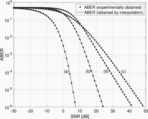
(a) The ABER curves of four different communications systems signaling using BPSK modulation in generalized fading environments. Referring to Section III-D, we choose $N=201$ and ${\bar{\gamma}}_{B}=100$ dB.

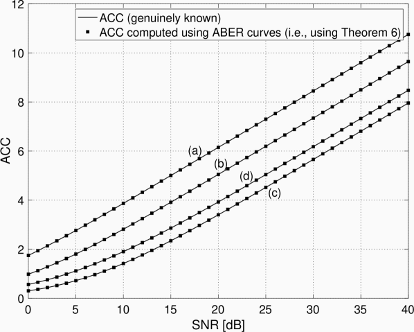
(b) The genie-aided ACC curves and the ACC results obtained from the ABER curves in generalized fading environments.

Figure 1: The numerical illustration of how the ACC of any communications system is readily obtained from its ABER curves for various SNR settings: $(a),\,(b),\,(c),\,(d)$ that are obviously not accounted in the numerical computation.

III-D ACC Analysis Using Empirical ABER Measurements

At the design and implementation stages of communications systems, it is crucial to empirically evaluate ACC to investigate the desired reliability of information transmission and to obtain conceptual results from practical and empirical perspectives. On the basis thereof and of using Theorem 6, we can readily calculate the ACC from the empirical ABER measurements for a binary modulation scheme. Let us assume that we obtain the measurement set $\mathcal{S}_{N}\!=\!\{({\bar{\gamma}}_{1},\mathcal{E}_{1}),({\bar{\gamma}}_{2},\mathcal{E}_{2}),\ldots,({\bar{\gamma}}_{N},\mathcal{E}_{N})\}$, where we have $\mathcal{E}_{n}\!=\!\mathcal{E}_{avg}\left({\bar{\gamma}}_{n}\right)$ for all $n\in\{1,2,\ldots,N\}$. Accordingly, using an efficient interpolation technique[25, 26, 27], we can accurately approximate $\mathcal{E}_{avg}\left({\bar{\gamma}}\right)$ as $\mathcal{E}_{avg}\left({\bar{\gamma}}\right)\approx\mathcal{E}_{int}\left({\bar{\gamma}}\,|\,\mathcal{S}_{N}\right)$ for any average SNR ${\bar{\gamma}}\in\mathbb{R}_{+}$. As well explained in Section II-B, we can efficiently apply the Lagrange’s interpolation to $\mathcal{S}_{N}$, and then we can write $\mathcal{E}_{int}\left({\bar{\gamma}}\,|\,\mathcal{S}_{N}\right)$ as

$$\mathcal{E}_{int}\left({\bar{\gamma}}\,|\,\mathcal{S}_{N}\right)=\sum_{n=1}^{N}\mathcal{E}_{n}\prod_{\begin{subarray}{c}k=1,\,{k}\neq{n}\end{subarray}}^{N}\frac{{\bar{\gamma}}-{\bar{\gamma}}_{k}}{{\bar{\gamma}}_{n}-{\bar{\gamma}}_{k}}.$$ (60)

Consequently, substituting (60) into (49), we can estimate the ACC $\mathcal{C}_{avg}\left({\bar{\gamma}}\right)$ from the empirical ABER measurements. For example, some ABER curves of communications systems are depicted in Fig. 1(a) for BPSK signalling in generalized fading environments, and the corresponding genie-aided ACC curves are depicted in Fig. 1(b). Fortunately, with the aid of Theorem 6, and without the need for the additional information for those ABER curves, we calculate each ACC curve from the corresponding ABER curve and plot in Fig. 1(b) the calculated ACC curves. Further, in Fig. 1(b), we notice that the calculated ACC curves are in perfect agreement with the genie-aided curves as expected. In addition, we illustrate in Fig. 2 the ACC versus the ABER. We notice therein the matter fact that ACC is a linear function of the logarithm of ABER when the ABER approaches zero (i.e., when the average SNR ${\bar{\gamma}}$ increases). However, this linearity is impaired for low averageSNR values. From this point of view, using the definition of low- and high-SNR regimes[12], we can conclude that the ACC of any communications system is determined by its ABER in low-SNR regime rather than in high-SNR regime.

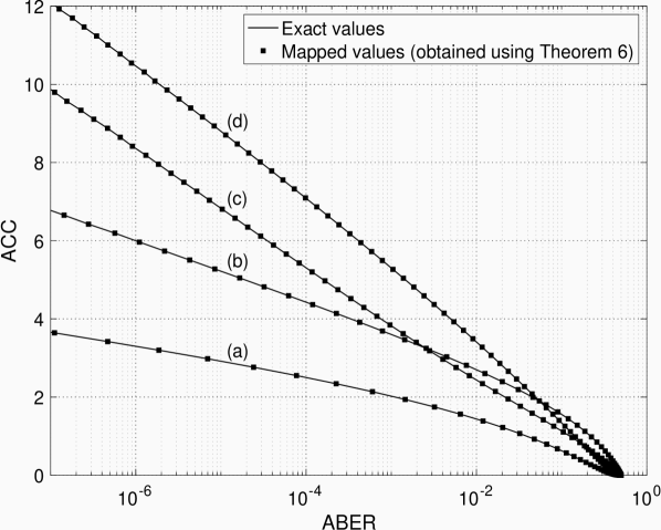
Figure 2: The relationship between the ACC and the ABER for a wireless communication system whose ABER curves are given in Fig. 1(a) for various SNR settings.

IV OP and OC Analyses Using ABER

Particularly when the fading conditions vary slowly, a possible deep fading has the potential to affect many successive bits during information transmission, resulting in large error bursts. If these errors cannot be corrected even if very complex coding and detection schemes are employed, the transmission channel will become unusable. In that context, the OP, denoted by $\mathcal{P}_{out}({\bar{\gamma}};\gamma_{th})$, is a channel quality measure[3, 4], defined as the probability that the SNR $\gamma$ drops below a certain threshold $\gamma_{th}$ for a certain average SNR ${\bar{\gamma}}$, that is defined as

$$\mathcal{P}_{out}({\bar{\gamma}};\gamma_{th})={\,{\mathbb{E}}\!\left[{\theta\!\left(\gamma_{th}-\gamma\right)}\right]},$$ (61)

for $\gamma\in\mathbb{R}^{+}$ and $\gamma_{th}\in\mathbb{R}^{+}$, where $\theta\!\left(\cdot\right)$ is Heaviside’s theta function (i.e., unit-step function) defined in [17, Eq. (1.8.3)],[42, Eq. (14.05.07.0002.01)], that is,

$$\theta\!\left(\gamma_{th}-\gamma\right)=\textstyle\begin{cases}1&\gamma<\gamma_{th}\\ \frac{1}{2}&\gamma=\gamma_{th}\\ 0&\gamma>\gamma_{th}\end{cases}.$$ (62)

Note that the exact OP analysis in (61), i.e., $\mathcal{P}_{out}({\bar{\gamma}};\gamma_{th})$ requires the SNR distribution. However, we demonstrate how we obtain the OP of any communications system by using its exact ACC performance, in particular without the knowledge of the SNR distribution and the underlying SNR settings.

Theorem 7 (OP analysis using ACC).

The OP $\mathcal{P}_{out}({\bar{\gamma}};\gamma_{th})$ of a wireless communications system is obtained using its exact (not approximate) ACC $\mathcal{C}_{avg}({\bar{\gamma}})$, that is

$$\mathcal{P}_{out}({\bar{\gamma}};\gamma_{th})=1-\frac{1}{\pi}\Im\biggl{\{}\mathcal{C}_{avg}\left(\!-\frac{{\bar{\gamma}}}{\gamma_{th}}\right)\biggr{\}},$$ (63)

for a certain threshold $\gamma_{th}\in\mathbb{R}^{+}$, where $\Im\!\left\{{\cdot}\right\}$ gives the imaginary part of its argument. Further, for numerical stability, $\mathcal{C}_{avg}(-{\bar{\gamma}})\approx\mathcal{C}_{avg}(e^{\varepsilon+{\rm{i}}\pi}{{\bar{\gamma}}})$, where we choose $\varepsilon\approx{0.0001}$.

Proof.

Due to the discordance between the monotonic natures of OP and ACC (i.e. since $\mathcal{P}_{out}({\bar{\gamma}};\gamma_{th})\geq\mathcal{P}_{out}({\bar{\gamma}}+\Delta{\bar{\gamma}};\gamma_{th})$ and $\mathcal{C}_{avg}({\bar{\gamma}})\leq\mathcal{C}_{avg}({\bar{\gamma}}+\Delta{\bar{\gamma}})$ for all $\Delta{\bar{\gamma}}\in\mathbb{R}_{+}$), both the OP and the ACC together do not preserve the same scaling order according to Theorem 5, and thus their LDS spectrums do not exist for a mutually common Hurst’s exponent. But, we write

$$\mathcal{P}_{out}({\bar{\gamma}};\gamma_{th})=1-\widehat{\mathcal{P}}_{out}({\bar{\gamma}};\gamma_{th}),$$ (64)

where $\widehat{\mathcal{P}}_{out}({\bar{\gamma}};\gamma_{th})$ is the complementary OP, defined as

$$\widehat{\mathcal{P}}_{out}({\bar{\gamma}};\gamma_{th})={\,{\mathbb{E}}\!\left[{\theta\!\left(\gamma-\gamma_{th}\right)}\right]},$$ (65)

which is monotonically increasing with respect to the average SNR ${\bar{\gamma}}$ (i.e., $\widehat{\mathcal{P}}_{out}({\bar{\gamma}};\gamma_{th})\leq\widehat{\mathcal{P}}_{out}({\bar{\gamma}}+\Delta{\bar{\gamma}};\gamma_{th})$). Therefore, the LDS of $\widehat{\mathcal{P}}_{out}({\bar{\gamma}};\gamma_{th})$ and that of $\mathcal{C}_{avg}({\bar{\gamma}})$ exist for a mutually common Hurst’s exponent. As is required for Theorem 5, we have already obtained in (51c) the LDS of $\mathcal{C}_{avg}({\bar{\gamma}})$ for Hurst’s exponent $0\!<\!H\!<\!1$, and moreover using [45, Eq. (2.2.1/1)], we obtain the LDS of the complementary OP as

$$\widetilde{\mathcal{P}}_{out}\left(\omega,{\bar{\gamma}}\right) = \mathfrak{F}_{\lambda}\!\bigl{\{}\mathfrak{L}^{-1}_{H,{\bar{\gamma}}}\bigl{\{}\widehat{\mathcal{P}}_{out}\left({\bar{\gamma}}\right)\bigr{\}}(\lambda)\bigl{\}}\left({\omega}\right),$$ (66a)

$$= \mu_{\gamma}(H+{\rm{i}}\,\omega;{\bar{\gamma}})\!\int_{0}^{\infty}\!\frac{\lambda^{-{\rm{i}}\,\omega}}{\lambda^{H+1}}\,\theta\left(\lambda-\gamma_{th}\right)d\lambda,{~{}~{}~{}~{}~{}~{}}$$ (66b)

$$= \mu_{\gamma}(H+{\rm{i}}\,\omega;{\bar{\gamma}})\,\gamma_{th}^{-H-{\rm{i}}\omega}{\left(H+{\rm{i}}\,\omega\right)}^{-1},$$ (66c)

for Hurst’s exponent $0\!<\!H\!<\!\infty$, where $\mu_{\gamma}(n;{\bar{\gamma}})\!=\!\mathbb{E}[\gamma^{n}]$ is the $n$th moment of the SNR distribution. Referring to Theorem 5, we find $\mathcal{Z}(u)$ by the ratio of (66c) to (51c), and then using [42, Eq. (06.05.16.0010.01)], we simplify it more to

$$\frac{\widetilde{\mathcal{P}}_{out}\left(\omega,{\bar{\gamma}}\right)}{\widetilde{\mathcal{C}}_{avg}\left(\omega,{\bar{\gamma}}\right)}=-\frac{1}{\pi}\sin(\pi(H+i\,\omega)),$$ (67)

which exists for Hurst’s exponent $0<H<1$. Replacing this ratio in (33) and changing the variable $H-{\rm{i}}\omega\rightarrow{s}$, we obtain

$$\mathcal{Z}(u)=\frac{1}{\pi}\Im\biggl{\{}\frac{1}{2\pi{\rm{i}}}\int_{-H-{\rm{i}}\,\infty}^{-H+{\rm{i}}\,\infty}u^{s-1}\bigl{(}-\gamma_{th}\bigr{)}^{s}ds\biggr{\}},$$ (68)

for $0\,\mathord{<}\,H\,\mathord{<}\,1$. Substituting (68) into (32), and therein changing the order of integrals and then exploiting MT, we obtain

$$\widehat{\mathcal{P}}_{out}({\bar{\gamma}};\gamma_{th})=\frac{1}{\pi}\Im\Bigl{\{}\mathcal{C}_{avg}\left(\!-{{\bar{\gamma}}}/{\gamma_{th}}\right)\Bigr{\}}.$$ (69)

Finally, exercising (64) and (69) together, we find (63), which completes the proof of Theorem 7. ∎

It is worth recalling that the OC, denoted by $\mathcal{C}_{out}({\bar{\gamma}};\gamma_{th})$, is defined as the probability that the instantaneous CC falls below a certain information rate $C_{th}$. As such, the CC while targeting a certain OP is called the OC performance, that is

$$\mathcal{C}_{out}({\bar{\gamma}};C_{th}) \mathrel{\overset{\makebox[0.0pt]{\mbox{\tiny$\!\triangle\!$}}}{=}} {\,{\mathbb{E}}\!\left[{\theta\!\left(C_{th}-\log(1+\gamma)\right)}\right]},$$ (70a)

$$= \mathcal{P}_{out}({\bar{\gamma}};e^{C_{th}}-1).$$ (70b)

Theorem 8 (OC analysis using ACC).

The OC $\mathcal{C}_{out}({\bar{\gamma}};\gamma_{th})$ of a wireless communications system is obtained using its exact (not approximate) ACC $\mathcal{C}_{avg}({\bar{\gamma}})$, that is

$$\mathcal{C}_{out}({\bar{\gamma}};C_{th})=1-\frac{1}{\pi}\Im\Bigl{\{}\mathcal{C}_{avg}\left(-{{\bar{\gamma}}}/{(e^{C_{th}}-1)}\right)\Bigr{\}}$$ (71)

for a certain capacity threshold $C_{th}\,\mathord{\in}\,\mathbb{R}^{+}$.

Proof.

The proof is obvious using (70b) in Theorem 7. ∎

IV-A OP and OC Analyses Using Exact ACC Expressions

The two novel relationships, which are proposed in Theorem 7 and Theorem 8, respectively, provide new insights into the OP and OC analyses of any communications system and show that an exact (non-approximate) ACC is sufficient for OP and OC analyses. Since neither integration nor further mathematical operations are required, these novel relationships, i.e., (63) and (71), are surely considered as closed-form expressions. However, in order to demonstrate their correctness, that is to derive the OP expressions from the closed-form ACC expressions in the literature, the hindrance in algebraic (mathematical) simplification is the elimination of imaginary-part operation. In more details, in the literature, the real-part and imaginary-part operations are not known to be expressed in terms of integral transforms. If they were known, the real-part and imaginary-part of higher transcendental functions (e.g., hypergeometric, Meijer’s G and Fox’s H functions) would be simplified to the expressions having no the real-part and imaginary-part operations. To the best of our knowledge, expressing real-part and imaginary-part operations in terms of integral transforms has so far not been reported in the literature. However, thanks to Theorem 4, we have rewritten them in terms of integral transforms in the following theorem.

Theorem 9 (Real-part and imaginary-part operations).

For a real-valued APM $\mathcal{G}_{avg}({\bar{\gamma}})$, $\Im\bigl{\{}\mathcal{G}_{avg}(-{\bar{\gamma}})\bigr{\}}$ and $\Re\bigl{\{}\mathcal{G}_{avg}(-{\bar{\gamma}})\bigr{\}}$ are respectively given by

$$\Im\bigl{\{}\mathcal{G}_{avg}(-{\bar{\gamma}})\bigr{\}} = \pi\,{\mathfrak{M}_{s}^{-{1}}\!\left\{{\frac{\mathfrak{M}_{{\bar{\gamma}}}\!\bigl{\{}\mathcal{G}_{avg}({\bar{\gamma}})\bigr{\}}\!\left(s\right)}{\Gamma\left(1+s\right)\Gamma\left(-s\right)}}\right\}\!\left({{\bar{\gamma}}}\right)},$$ (72)

$$\Re\bigl{\{}\mathcal{G}_{avg}(-{\bar{\gamma}})\bigr{\}} = \pi\,{\mathfrak{M}_{s}^{-{1}}\!\left\{{\frac{\mathfrak{M}_{{\bar{\gamma}}}\!\bigl{\{}\mathcal{G}_{avg}({\bar{\gamma}})\bigr{\}}\!\left(s\right)}{\Gamma\left(\frac{1}{2}+s\right)\Gamma\left(\frac{1}{2}-s\right)}}\right\}\!\left({{\bar{\gamma}}}\right)},{~{}~{}~{}}$$ (73)

where ${\mathfrak{M}_{\cdot}\!\left\{{\cdot}\right\}\!\left({\cdot}\right)}$ is the MT, and ${\mathfrak{M}_{\cdot}^{-{1}}\!\left\{{\cdot}\right\}\!\left({\cdot}\right)}$ is the IMT⁶.

Proof.

The proof is omitted due to space limitations. ∎

Although Theorem 8 is itself in closed form, let us consider some OP and OC examples in fading enviroments, clarifying the contribution of Theorem 9 to deriving closed-form expressions. The OP of a communications system signalling in Nakagami-m fading environments is given by [8, Eq. (33)]

$$C_{avg}\left({\bar{\gamma}}\right)=\frac{1}{\Gamma(m)}{\rm{G}}^{3,1}_{2,3}{\left[\left.{\frac{m}{{\bar{\gamma}}}}\right|\genfrac{}{}{0.0pt}{}{{0,1}}{{m,0,0}}\right]},$$ (74)

where the parameter $m$ denotes the fading figure (i.e., diversity order) ranging from $1/2$ to $\infty$[3, Section 2.2.1.4]. According to Theorem 7, we need to have $\Im\!\left\{{C_{avg}\left(-{\bar{\gamma}}\right)}\right\}$, and it can be found with the aid of Theorem 9, where we derive the MT of (74) using [23, Eq. (2.1.3)] and [23, Eq. (2.9.1)], that is ${\mathfrak{M}_{{\bar{\gamma}}}\!\left\{{C_{avg}\left({\bar{\gamma}}\right)}\right\}\!\left({s}\right)}=\allowbreak{-}{m}^{s}\Gamma(-s)\Gamma(s)\Gamma(m-s)/\Gamma(m)$, whose substitution into (72) yields

$$\Im\!\left\{{C_{avg}\left(-{\bar{\gamma}}\right)}\right\}=-\pi\,{\mathfrak{M}_{s}^{-{1}}\!\left\{{{m}^{s}\frac{\Gamma(m-s)}{s\,\Gamma(m)}}\right\}\!\left({{\bar{\gamma}}}\right)},$$ (75)

where using [40, Eq. (8.4.16/4)] results in $\Im\!\left\{{C_{avg}\left(-{\bar{\gamma}}\right)}\right\}=\pi{\Gamma(m,{m}/{{\bar{\gamma}}})}/{\Gamma(m)}$. Finally, substituting this result into (63) yields the well-known OP results[4, 2, 3],

$$P_{out}\left({\bar{\gamma}};\gamma_{th}\right)=1-\frac{\Gamma(m,{m}{\gamma_{th}}/{{\bar{\gamma}}})}{\Gamma(m)},$$ (76)

as expected. The OC $\mathcal{C}_{out}({\bar{\gamma}};C_{th})$ is easily obtained using (76) and (70b) together.

IV-B Obtaining SNR distribution Using Exact ACC Expressions

While the PDF of SNRs distribution, which is often referred to as sample (descriptive) statistics, reveals the relative likelihood of any sample in a continuum occurring, APMs provide a determination of what is most likely to be correct / incorrect with the evidence of sample statistics. The notion commonly followed in the literature is to obtain the APMs using sample statistics such as the PDF, CDF and MGF of SNR distribution. conversely, to the best of knowledge, how to obtain sample statistics from APMs has so far not been explored in the literature. In the following, we demonstrate that the exact (not approximate) ACC expression of any communications system is enough to determine the PDF of the SNR distribution to which overall information transmission is subjected.

Theorem 10 (PDF of SNR distribution using ACC).

Let $\mathcal{C}_{avg}({\bar{\gamma}})$ be the exact ACC of a wireless communication system whose SNR distribution follows the PDF $f_{\gamma}(r;{\bar{\gamma}})$. Accordingly, the PDF $f_{\gamma}(r;{\bar{\gamma}})$ is given by

$$f_{\gamma}(r;{\bar{\gamma}})=-\frac{1}{\pi}\Im\biggl{\{}\frac{\partial}{\partial{r}}\,\mathcal{C}_{avg}\left(-\frac{{\bar{\gamma}}}{r}\right)\biggr{\}},$$ (77)

defined over $r\in\mathbb{R}^{+}$.

Proof.

Note that, for the SNR distribution, which is denoted by $\gamma$, the PDF $f_{\gamma}(r)$ and the CDF $F_{\gamma}(r)$ are defined as

$$f_{\gamma}(r) = {\,{\mathbb{E}}\!\left[{{\,\mathord{\delta}\!\left({r-\gamma}\right)}}\right]},$$ (78)

$$F_{\gamma}(r) = {\,{\mathbb{E}}\!\left[{{\,\mathord{\theta}\!}\left({r-\gamma}\right)}\right]},$$ (79)

respectively. Using [46, Eq. (19.1.3.1/3)], we rewrite the PDF $f_{\gamma}(r)$ in terms of the CDF $F_{\gamma}(r)$, that is

$$f_{\gamma}(r)=\frac{\partial}{\partial{r}}F_{\gamma}(r).$$ (80)

Finally, noticing $F_{\gamma}(\gamma_{th})\mathrel{\overset{\makebox[0.0pt]{\mbox{\tiny$\!\triangle\!$}}}{=}}\mathcal{P}_{out}({\bar{\gamma}};\gamma_{th})$ from (61) and (79), and subsequently substituting (80) into (63), we deduce (77), which proves Theorem 10. ∎

In the literature of communications theory, there are several studies and publications about APM analyses that widely use two approaches; one of which is the PDF-based approach[2, and references therein] that requires an exact or approximated PDF of SNR distribution. The other one is the MGF-based approach[3, and references therein] that requires an exact or approximated MGF of SNR distribution for the APM analyses of a diversity receiver with an arbitrary number of diversity branches over a variety of fading channels. In addition to these two approaches, with the aid of Theorem 10, we propose in the following theorem a novel approach which we call the CC-based approach. Moreover, we show that the exact (non-approximate) ACC is sufficient and enough to achieve all APM analyses, especially without requiring the statistical knowledge (e.g., PDF, CDF, MGF, or moments) of the SNR distribution.

Theorem 11 (CC-Based Performance Analysis).

Let $\mathcal{H}(\gamma)$ be a PM according to the SNR distribution $\gamma$. The corresponding APM defined as $\mathcal{H}_{avg}({\bar{\gamma}})\mathrel{\overset{\makebox[0.0pt]{\mbox{\tiny$\!\triangle\!$}}}{=}}{\,{\mathbb{E}}\!\left[{\mathcal{H}(\gamma)}\right]}$ is given by

$$\mathcal{H}_{avg}({\bar{\gamma}})=\mathcal{H}\left(0\right)+\frac{1}{\pi}\int_{0}^{\infty}\mathcal{H}^{\prime}\!\left(r\right)\Im\biggl{\{}\mathcal{C}_{avg}\left(\!-\frac{{\bar{\gamma}}}{r}\right)\biggr{\}}d{r},$$ (81)

for an average SNR ${\bar{\gamma}}$, where $\mathcal{H}^{\prime}\!\left(\gamma\right)=\frac{\partial}{\partial\gamma}\mathcal{H}\left(\gamma\right)$.

Proof.

Using the PDF-based approach when the PDF $f_{\gamma}(r;{\bar{\gamma}})$ is expressed in closed-form expression, we rewrite the APM $\mathcal{H}_{avg}({\bar{\gamma}})$ as follows

$$\mathcal{H}_{avg}({\bar{\gamma}})=-\int_{0}^{\infty}\mathcal{H}\left(r\right)\,\frac{\partial}{\partial{r}}\widehat{\mathcal{P}}_{out}({\bar{\gamma}};r)\,d{r},$$ (82)

where $\widehat{\mathcal{P}}_{out}({\bar{\gamma}};\gamma_{th})$ is the complementary OP. Consequently, using integration-by-part [17, Eq. (5.3.11)] and therein noticing $\lim_{r\rightarrow{0}}\widehat{\mathcal{P}}_{out}({\bar{\gamma}};r)\,\mathord{=}\,{1}$ and $\lim_{r\rightarrow\infty}\widehat{\mathcal{P}}_{out}({\bar{\gamma}};r)\,\mathord{=}\,{0}$, we obtain (81), which proves Theorem 11. ∎

For the analytical accuracy and correctness of Theorem 11, let us consider an extreme example of the ABER $\mathcal{E}_{avg}({\bar{\gamma}})$ of a communications system signalling over cascaded Generalized Nakagami-$m$ (GNM) fading channels[47]. The corresponding ACC is given by [47, Eq. (33)]

$$\!\!\!\!\mathcal{C}_{avg}({\bar{\gamma}})={\rm{H}}^{N+2,1}_{N+2,N+2}{\left[\left.{\frac{1}{{\bar{\gamma}}}{\prod\limits_{\ell=1}^{N}{{\beta_{\ell}}}}}\right|\genfrac{}{}{0.0pt}{}{{(0,1),(1,1),\Psi^{(0)}_{N}}}{{\Psi^{(1)}_{N},(0,1),(0,1)}}\right]},\!\!$$ (83)

where ${\rm{H}}^{m,n}_{p,q}{\left[\cdot\right]}$ denotes the Fox’s H’ function[23, Eq. (1.1.1)],[40, Eq. (8.3.1/1)], $N$ denotes the hop number in the transmission, and $\Psi^{(n)}_{N}\!=\!(m_{1},{n}/{\xi_{1}}),(m_{2},{n}/{\xi_{2}}),\allowbreak\ldots,(m_{N},{n}/{\xi_{N}})$. In addition, for all $\ell\in\{1,2,\ldots,N\}$, $\beta_{\ell}=\Gamma(m_{\ell}+1/\xi_{\ell})/\Gamma(m_{\ell})$, where $m_{\ell}$ and $\xi_{\ell}$ denote the fading figure (i.e., the diversity order) and the shape parameter of the $\ell$th hop, respectively. With the aid of Theorem 11, we do not necessitate the statistical knowledge of SNR distribution for the ABER analysis. As such, using the closed-form ACC that is given in (83), we can write the ABER $\mathcal{E}_{avg}({\bar{\gamma}})$ as follows

$$\mathcal{E}_{avg}({\bar{\gamma}})=\mathcal{E}\left(0\right)+\frac{1}{\pi}\int_{0}^{\infty}\mathcal{E}^{\prime}\!\left(r\right)\Im\biggl{\{}\mathcal{C}_{avg}\left(\!-\frac{{\bar{\gamma}}}{r}\right)\biggr{\}}d{r},$$ (84)

where $\mathcal{E}\left(\gamma\right)$ is the PM defined by $\mathcal{E}\left(\gamma\right)\!=\!{\Gamma\left(b,a\,\gamma\right)}/{\Gamma\left(b\right)}/2$ with parameters $a,b\!\in\!\{1/2,1\}$ (see Section III-A for further details). We have $\lim_{\gamma\rightarrow{0}}\mathcal{E}(\gamma)\!=\!1/2$ and $\lim_{\gamma\rightarrow{\infty}}\mathcal{E}(\gamma)\!=\!0$. Further, using [42, Eq. (06.06.20.0003.01)] and [23, Eqs. (1.1.1) and (2.5.7)], we have

$$\frac{\partial}{\partial\gamma}\mathcal{E}\left(\gamma\right)=\frac{a}{2\Gamma(b)}{\rm{H}}^{1,0}_{0,1}{\left[{a\gamma}\left|\genfrac{}{}{0.0pt}{}{{\raisebox{2.13394pt}{\rule{16.0pt}{0.4pt}}}}{{(b-1,1)}}\right.\right]},$$ (85)

In addition, we obtain the MT of (83) using the MT of Fox’s H function[48, Eq. (8.3.1/1)] and [23, Eq. (8.3.1/1)]. Thereafter, substituting it into (72), we obtain

$$\!\!\!\!\Im\Bigl{\{}\mathcal{C}_{avg}(-{\bar{\gamma}})\Bigr{\}}=\pi{\rm{H}}^{N,N+1}_{1,N+1}{\left[\left.{\frac{1}{\bar{\gamma}}{\prod\limits_{\ell=1}^{N}{{\beta_{\ell}}}}}\right|\genfrac{}{}{0.0pt}{}{{(0,1),\Psi^{(0)}_{N}}}{{\Psi^{(1)}_{N},(0,1)}}\right]},\!\!$$ (86)

Finally, substituting both (85) and (86) into (84) and therein employing Mellin’s convolution of Fox’s H functions[23, Eq. (2.8.11)], we obtain the ABER $\mathcal{E}_{avg}({\bar{\gamma}})$ for binary modulation schemes over cascaded GNM fading channels as

$$\!\!\!\!\mathcal{E}_{avg}({\bar{\gamma}})=\frac{1}{2}{\rm{H}}^{N,2}_{N+2,N+2}{\left[{\frac{1}{a\bar{\gamma}}\prod\limits_{\ell=1}^{N}{\beta_{\ell}}}\left|\genfrac{}{}{0.0pt}{}{{(1-b,1),(1,1),\Psi^{(0)}_{N}}}{{\Psi^{(1)}_{N},(0,1),(1-b,0)}}\right.\right]},\!\!$$ (87)

which is in perfect agreement with [47, Eq. (40)] as expected. This example clearly demonstrates how we can benefit from ACC performance to obtain other APMs without knowing the SNR distribution. The number of such examples can easily be increased by considering other closed-form ACC expressions available in the literature.

V Conclusion

In this article, we first recommend the use of LT to facilitate self-similarity (scale invariance) and therefrom introduce the LDS spectrums to identify the similarity between any two APMs. Secondly, we propose a tractable approach, which we call LT-based approach for performance analysis, to establish a relationship between any two APMs. As such, we demonstrate how to compute one APM using the other APM, especially without needing the statistical knowledge (such as PDF, CDF, MGF and moments) of SNR distribution and knowing the broadest SNR settings.

To the best of our knowledge, the literature has currently no answer on how we determine ACC either empirically or experimentally without using the statistical knowledge of SNR distribution. As regards an application of our LT-based approach, we propose a relationship in which we can predict the ACC of any communications system using its ABER performance that we can empirically measure without the need for the statistical knowledge of SNR distribution and all the SNR settings.

In addition, we show for the first time in the literature how to obtain sample statistics (such as PDF, CDF and MGF of SNR distribution) from APMs, which changes the playground of performance analysis in the field of wireless communications. We propose that both OP and OC of any communications system can be obtained by using its exact ACC performance. To the best of our knowledge, this relationship has also not been yet reported in the literature. In addition, we introduce a novel approach, which we call the CC-based approach to perform any APM analysis using the exact ACC expressions.

Finally, considering some extreme examples, we illustrate the usages and usefulness of our newly proposed relationships. Performing Monte-Carlo simulations, we validate their accuracy and consistency.

Ferkan Yilmaz (SM’2004–M’2009) received the B.Sc. degree in electronics and communications engineering from Yıldız Technical University, Turkey, in 1997. He was ranked the first among all undergraduate students who graduated from the Department of Electronics and Communication Engineering (ECE), and the second among all undergraduate students who graduated in 1997 from Yıldız Technical University. He received his M.Sc. degree in the field of electronics and communications from Istanbul Technical University, Turkey, in 2002, and the Ph.D. degree in field of wireless communications from Gebze Institute of Technology (GYTE) in 2009. He was awarded for the best Ph.D. Thesis. From 1998 to 2003, he worked as a researcher for National Research Institute of Electronics and Cryptology, TÜBİTAK, Turkey. Dr. Yilmaz is the recipient of The 1999 Achievement Award from TÜBİTAK. From 2003 to 2008, he worked as a senior Telecommunications Engineer for Vodafone Technology, Turkey. In November 2008, he was invited by Prof. Dr. M.-S. Alouini to work as a visitor researcher at Texas A&M University (Qatar), and from August 2009 till November 2012, worked as a post-doctoral fellow at King Abdullah University of Science and Technology (KAUST). Between November 2012 and April 2015, he joined as a Senior Telecommunications expert in the Location-based Service Solutions group, Vodafone Technology, and therein developed positioning algorithms and achieved the implementation and assessment of indoor / outdoor location-aware applications. In 2015, he was with KAUST as a Remote Consultant working on optical communications. In 2016, Dr. Yilmaz joined to the Department of Computer Engineering at Yıldız Technical University. He has been currently working as a Assistant Professor and also engaged in Alpharabius Solutions and Tachyonic Solutions startup companies. He served as a TPC member for several IEEE conferences and is a regular reviewer for various IEEE journals. His research interests focus on wireless communication theory (i.e, diversity techniques, cooperative communications, spatial modulation, fading channels), signal processing, stochastic random processes, statistical learning theory, and machine learning and data mining (big data, data analytics).

References

• [1] Dongning Guo, S. Shamai, and S. Verdu, “Mutual information and minimum mean-square error in Gaussian channels,” IEEE Trans. Inf. Theory, vol. 51, no. 4, pp. 1261–1282, 2005.
• [2] J. Proakis, Digital Communications, 4th ed.   McGraw-Hill Science/Engineering/Math, Aug. 2000.
• [3] M. K. Simon and M.-S. Alouini, Digital Communication over Fading Channels, 2nd ed.   John Wiley & Sons, Inc., 2005.
• [4] A. Goldsmith, Wireless Communications.   Cambridge University Press, Aug.8, 2005.
• [5] M. K. Simon and M.-S. Alouini, “A unified approach to the performance analysis of digital communication over generalized fading channels,” Proceedings of the IEEE, vol. 86, no. 9, pp. 1860–1877, Sep. 1998.
• [6] A. Annamalai, C. Tellambura, and V. K. Bhargava, “A general method for calculating error probabilities over fading channels,” IEEE Trans. Commun., vol. 53, no. 5, pp. 841–852, May 2005.
• [7] F. Yilmaz and M.-S. Alouini, “A novel ergodic capacity analysis of diversity combining and multihop transmission systems over generalized composite fading channels,” in proc. IEEE International Conference on Communications (ICC 2012), Ottawa, Canada, June 2012, pp. 4605–4610.
• [8] ——, “A unified MGF-based capacity analysis of diversity combiners over generalized fading channels,” IEEE Trans. Commun., vol. 60, no. 3, pp. 862–875, Mar. 2012.
• [9] ——, “A novel unified expression for the capacity and bit error probability of wireless communication systems over generalized fading channels,” IEEE Trans. Commun., vol. 60, no. 7, pp. 1862–1876, 2012.
• [10] ——, “On the computation of the higher-order statistics of the channel capacity over generalized fading channels,” IEEE Wireless Communications Letters, vol. 1, no. 6, pp. 573–576, 2012.
• [11] ——, “Novel asymptotic results on the high-order statistics of the channel capacity over generalized fading channels,” in IEEE Inter. Workshop on Signal Processing Advances in Wireless Commun. (SPAWC 2012), 2012, pp. 389–393.
• [12] F. Yilmaz, “On the asymptotic analysis of the high-order statistics of the channel capacity over generalized fading channels,” Turkish Journal of Electrical Engineering & Computer Sciences, 2019, Accepted for publication.
• [13] J. Lamperti, “Semi-stable stochastic processes,” Transactions of the American Mathematical Society, vol. 104, pp. 62–78, 1962.
• [14] C. E. Shannon, “A mathematical theory of communication,” Bell System Tech. Journal, vol. 27, pp. 379–423, 623–656, Julyand Oct. 1948, Available at http://cm.bell-labs.com/cm/ms/what/shannonday/paper.html.
• [15] ——, “Communications in the presence of noise,” in Proc. IRE, 1949, pp. 10–21.
• [16] C. E. Shannon and W. Weaver, The Mathematical Theory of Communication.   Urbana, IL, USA: University of Illinois Press, 1949.
• [17] D. Zwillinger, CRC Standard Mathematical Tables and Formulae, 31st ed.   Boca Raton, FL: Chapman & Hall/CRC, 2003.
• [18] B. B. Mandelbrot, The fractal geometry of nature, 1st ed.   W.H. Freeman, Aug 1982.
• [19] D. C. Champeney, A handbook of Fourier theorems.   Cambridge University Press, 1987.
• [20] I. N. Sneddon, Fourier Transforms, ser. Dover Books on Mathematics.   Dover Publications, 1995.
• [21] F. Oberhettinger, Tables of Mellin Transforms.   Springer-Verlag, 1974.
• [22] A. D. Poularikas, The Transforms and Applications Handbook, ser. The Electrical Engineering Handbook Series.   CRC Press, 2000.
• [23] A. Kilbas and M. Saigo, H-Transforms: Theory and Applications.   Boca Raton, FL: CRC Press LLC, 2004.
• [24] A. M. Mathai, R. K. Saxena, and H. J. Haubold, The H-Function: Theory and Applications.   New York Dordrecht Heidelberg London: Springer, 2010.
• [25] P. J. Davis, Interpolation and approximation.   Courier Corporation, 1975.
• [26] W. H. Press, S. A. Teukolsky, W. T. Vetterling, and B. P. Flannery, Numerical Recipes in C - The Art of Scientific Computing, 2nd ed.   Cambridge, U.K.: Cambridge University., 1992.
• [27] S. S. M. Wong, Computational Methods in Physics and Engineering, 2nd ed.   Upper Saddle River, NJ: World Scientific, 1997.
• [28] W. C. Y. Lee, “Estimate of channel capacity in Rayleigh fading environment,” IEEE Trans. Veh. Technol., vol. 39, no. 3, pp. 187–189, Aug. 1990.
• [29] T. Ericson, “A Gaussian channel with slow fading (Corresp.),” IEEE Trans. Inf. Theory, vol. 16, no. 3, pp. 353–355, May 1970.
• [30] L. H. Ozarow, S. Shamai, and A. D. Wyner, “Information theoretic considerations for cellular mobile radio,” IEEE Trans. Veh. Technol., vol. 43, no. 2, pp. 359–378, May 1994.
• [31] A. J. Goldsmith and P. P. Varaiya, “Capacity of fading channels with channel side information,” IEEE Trans. Inf. Theory, vol. 43, no. 6, pp. 1986–1992, Nov. 1997.
• [32] M.-S. Alouini and A. J. Goldsmith, “Capacity of Rayleigh fading channels under different adaptive transmission and diversity-combining techniques,” IEEE Trans. Veh. Technol., vol. 48, no. 4, pp. 1165–1181, July 1999.
• [33] ——, “Adaptive modulation over Nakagami fading channels,” Wireless Personal Commun., vol. 13, pp. 119–143, 2000.
• [34] H. Viswanathan, “Capacity of Markov channels with receiver CSI and delayed feedback,” IEEE Trans. Inf. Theory, vol. 45, no. 2, pp. 761–771, Mar. 1999.
• [35] S. K. Jayaweera and H. V. Poor, “Capacity of multiple-antenna systems with both receiver and transmitter channel state information,” IEEE Trans. Inf. Theory, vol. 49, no. 10, pp. 2697–2709, Oct. 2003.
• [36] Yuan Zhang and C. Tepedelenlioglu, “Asymptotic capacity analysis for adaptive transmission schemes under general fading distributions,” IEEE Trans. Inf. Theory, vol. 58, no. 2, pp. 897–908, Feb. 2012.
• [37] M.-S. Alouini and A. J. Goldsmith, “A unified approach for calculating error rates of linearly modulated signals over generalized fading channels,” IEEE Trans. Commun., vol. 47, no. 9, pp. 1324–1334, Sep. 1999.
• [38] A. Wojnar, “Unknown bounds on performance in Nakagami channels,” IEEE Trans. Commun., vol. 34, no. 1, pp. 22–24, Jan. 1986.
• [39] M. Abramowitz and I. A. Stegun, Handbook of Mathematical Functions with Formulas, Graphs, and Mathematical Tables, 9th ed.   New York: Dover Publications, 1972.
• [40] A. P. Prudnikov, Y. A. Brychkov, and O. I. Marichev, Integral and Series: Volume 3, More Special Functions.   CRC Press Inc., 1990.
• [41] I. S. Gradshteyn and I. M. Ryzhik, Table of Integrals, Series, and Products, 5th ed.   San Diego, CA: Academic Press, 1994.
• [42] Wolfram Research, Mathematica Edition: Version 8.0.   Champaign, Illinois: Wolfram Research, Inc., 2010.
• [43] A. P. Prudnikov, Y. A. Brychkov, and O. I. Marichev, Integral and Series: Volume 2, Special Functions.   CRC Press Inc., 1990.
• [44] V. Aalo, T. Piboongungon, and C.-D. Iskander, “Bit-error rate of binary digital modulation schemes in generalized Gamma fading channels,” IEEE Commun. Lett., vol. 9, no. 2, pp. 139–141, Feb. 2005.
• [45] A. P. Prudnikov, Y. A. Brychkov, and O. I. Marichev, Integral and Series: Volume 4, Direct Laplace Transforms.   CRC Press Inc., 1990.
• [46] A. Jeffrey and H.-H. Dai, Handbook of Mathematical Formulas and Integrals, 4th ed.   Academic Press, 2008.
• [47] F. Yilmaz and M.-S. Alouini, “Product of the powers of generalized nakagami-m variates and performance of cascaded fading channels,” in proc. IEEE Global Communications Conference (GLOBECOM 2009), Honolulu, Hawaii, USA, Nov. 30-Dec. 4 2009.
• [48] A. P. Prudnikov, Y. A. Brychkov, and O. I. Marichev, Integral and Series: Volume 1, Elementary Functions.   CRC Press Inc., 1990.