Hot quark matter and (proto-) neutron stars

Abstract

In part one of this paper, we use a non-local extension of the 3-flavor Polyakov-Nambu-Jona-Lasinio model, which takes into account flavor-mixing, momentum dependent quark masses, and vector interactions among quarks, to investigate the possible existence of a spinodal region (determined by the vanishing of the speed of sound) in the QCD phase diagram and determine the temperature and chemical potential of the critical end point. In part two of the paper, we investigate the quark-hadron composition of baryonic matter at zero as well as non-zero temperature. This is of great topical interest for the analysis and interpretation of neutron star merger events such as GW170817. With this in mind, we determine the composition of proto-neutron star matter for entropies and lepton fractions that are typical of such matter. These compositions are used to delineate the evolution of proto-neutron stars to neutron stars in the baryon-mass versus gravitational-mass diagram. The hot stellar models turn out to contain significant fractions of hyperons and $\Delta$-isobars but no deconfined quarks. The latter, are found to exist only in cold neutron stars.

I Introduction

Exploring the thermodynamic behavior of the quark-gluon plasma and its associated equation of state (EoS) has become one of the forefront areas of modern physics. The properties of such matter are being probed with the Relativistic Heavy Ion Collider (RHIC) at BNL and the Large Hadron Collider (LHC) at CERN, and great advances in our understanding of such matter are expected from the next generation of high density experiments at the Facility for Antiproton and Ion Research (FAIR at GSI) B. Friman and C. Höhne and J. Knoll and S. Leupold and J. Randrup and R. Rapp and P. Senger, (2011) (Eds.); FAI , the Nuclotron-bases Ion Collider fAcility (NICA at JINR) Blaschke et al. (2016); NIC , the Japan Proton Accelerator Research Complex (J-PARC at Tokai campus of JAEA) J-P , the Super Proton Synchrotron (SPS at CERN) SPS and the Beam Energy Scan (BES at BNL) BES .

Depending on temperature $T$, and baryon chemical potential $\mu$, the deconfined phase of quarks and gluons is believed to exist at two extreme regions in the phase diagram of quantum chromodynamics (QCD). The first regime corresponds to $T>>\mu$, which was the case in the early Universe where the temperature was hundreds of MeV but the net baryon number density was very low. Secondly, it is theorized that quark deconfinement occurs also at low temperatures but very high chemical potential, $T<<\mu$, that is, at conditions which exist in the inner cores of (proto-) neutron stars Roark and Dexheimer (2018). Portions of the phase diagram lying between these two extreme physical regimes can be probed with relativistic collision experiments.

Effective field-theoretical models such as the Nambu-Jona-Lasinio model and its extensions Buballa (2005); Fukushima (2008a); Contrera et al. (2008); Contrera, G. A. and Orsaria, M. and Scoccola, N. N. (2010); Carlomagno (2018) as well as lattice QCD (LQCD) calculations Philipsen (2013); Borsanyi et al. (2014); Bellwied et al. (2015) predict a smooth crossover of nuclear matter to quark matter in the low density but high temperature regime of the phase diagram. On the other hand, in the low temperature but high chemical potential regime the hadron-quark phase transition is likely be of first-order Fukushima and Hatsuda (2011). Some recent works Most et al. (2019); Bauswein et al. (2019) have investigated the occurrence of a first order phase transition in neutron-star mergers.

Spinodal instabilities are characteristic features in systems which exhibit first-order phase transitions. If present in the quark gluon plasma, spinodal instabilities would lead to density fluctuations that have a qualitative influence on the dynamical evolution of the system density Steinheimer, Jan and Randrup, Jørgen (2012). The fluctuations that lead to a spinodal decomposition are long range and differ from local fluctuations that give rise to nucleation, which occurs in the metastable region of the phase diagram. Hence, if there is a first-order phase transition, large density fluctuations can arise as a result of spinodal instabilities. The effects of spinodal instabilities in nuclear collision simulations at NICA energy densities were studied in Steinheimer and Randrup (2016). The spinodal region has also been analyzed for two Sasaki, C. and Friman, B. and Redlich, K. (2007, 2008) and three Li, Feng and Ko, Che Ming (2017) flavor quark matter using the local Nambu-Jona-Lasinio (NJL) model.

In this work, we investigate the hadron-quark phase transition in superdense matter and the possible appearance of deconfined quark matter in the cores of (proto-) neutron stars. For the description of quark matter we use the non-local SU(3) NJL model coupled to the Polyakov loop (hereafter referred to a 3nPNJL model). Vector interactions among quark are taken into account too. The use of non-local interactions has been suggested as an improvement of the standard NJL model. Non-locality arises naturally from several successful approaches to low-energy quark dynamics, such as one-gluon exchange descriptions Contrera et al. (2008); Contrera, G. A. and Orsaria, M. and Scoccola, N. N. (2010), the instanton liquid model Schaefer and Shuryak (1998), and the Schwinger-Dyson resummation techniques Roberts and Schmidt (2000).

We calculate the metastable regions of the phase diagram and investigate the possible existence of quark-hybrid stars assuming a sharp hadron-quark phase transition. Hadronic matter is assumed to be made of neutrons, protons, hyperons, and delta isobars. The field equations of these particles are solved for an improved parametrization of the relativistic mean-field model with density dependent coupling constants. The density at which quark deconfinement may occur in the cores of neutron stars is assumed to be several times greater than the saturation density of ordinary nuclear matter. The equations of state computed in this work fulfill the $2M_{\odot}$ mass constraints set by PSR J1614-2230 and PSR J0348+0432 Demorest et al. (2010); Lynch et al. (2013); Antoniadis et al. (2013); Arzoumanian et al. (2018) as well as the radius constraints derived from the gravitational-wave event GW170817 and its electromagnetic counterpart GRB 170817A Bauswein et al. (2017); Fattoyev et al. (2018); Raithel et al. (2018a); Most et al. (2018a); Annala et al. (2018).

The article is organized as follows. In Section II, we provide a description of the 3nPNJL model and its parameterizations, pointing out some of the reasons for using a non-local model instead of the local one. We analyze the structure of the phase diagram as predicted by the 3nPNJL model and explore the occurrence of a spinodal region, which is determined by the vanishing of the speed of sound. Section III is devoted to the description of hadronic matter. In Section IV, we discuss the transition of hadronic matter to quark matter and present the properties of neutron stars computed for the EoS of this work. The study of several selected stages in the evolution of proto-neutron stars to neutron stars is given in Section V. Finally, Section VI provides a summary of the results and some conclusions.

II Quark matter at finite temperature

II.1 The local vs the non-local NJL model

The standard NJL model is based on an effective lagrangian of relativistic fermions interacting through local fermion-fermion couplings. Because of the local nature of the interaction, the Schwinger-Dyson and Bethe-Salpeter equations become relatively simple. However, one of the drawbacks of the model is that it is non-renormalizable. The problems of ultra-violet divergences for this model can be fixed by using non-local rather than local interactions. Furthermore, the local NJL model works with an artificial momentum-space cutoff of $\Lambda\sim 0.6-0.7$ GeV, which is turned off at high momenta. Thus, the applicability of this model is restricted to energy and momentum scales (temperatures, chemical potentials) that are small compared to $\Lambda$. Connections to the running QCD coupling constant and the established high-momentum, high-temperature behavior governed by perturbative QCD are therefore ruled out right from the start.

In this work we will consider the 3nPNJL model, which includes vector interactions among quarks. Non-local extensions of the NJL model are designed to remove the deficiencies of the local model, while, at the same time, the non-local interactions regularize the model in such a way that the basic features of a relativistic quark matter system, like chiral symmetry breaking and the formation of bound stages in the low-energy limit, can be properly described (see Contrera, G. A. and Orsaria, M. and Scoccola, N. N. (2010) and references therein). In addition, the range (in momentum space) of the non-locality provides a natural cutoff that falls off at high densities, which makes the model more appropriate for the description of quark matter than the local NJL model, even in the perturbative regime.

II.2 The 3nPNJL model

To study the QCD phase diagram and the EoS with the 3nPNJL model, we start from the lagrangian

$$\mathcal{L}(x) = \bar{\psi}(x)(-i\not{D}+\hat{m})\psi(x)+\frac{G_{V}}{2}j_{a}^{\mu}(x)j_{a}^{\mu}(x)$$

$$- \frac{G_{S}}{2}\big{[}j_{a}^{s}(x)j_{a}^{s}(x)+j_{a}^{p}(x)j_{a}^{p}(x)\big{]}+{\cal U}\,[{\cal A}(x)]$$

$$- \frac{H}{4}A_{abc}\big{[}j_{a}^{s}(x)j_{b}^{s}(x)j_{c}^{s}(x)-3j_{a}^{s}(x)j_{b}^{p}(x)j_{c}^{p}(x)\big{]},$$

which accounts for scalar as well as vector interactions among quarks. The quantity ${\cal U}$ is an effective potential which accounts for Polyakov loop dynamics, and the last term denotes the ’tHooft term which is responsible for flavor mixing. The quantities $\psi$ denotes the light quark fields, $\psi\equiv(u\;d\;s)^{T}$, and $\hat{m}={\rm diag}(m_{u},m_{d},m_{s})$ stands for the current quark mass matrix. For simplicity we consider the isospin symmetric limit where $m_{u}=m_{d}$.

Regarding the interaction terms, the scalar ($s$), pseudo scalar ($p$) and vector ($\mu$) interaction currents are respectively given by

$$j_{a}^{s}(x) = \int d^{4}z\tilde{R}(z)\bar{\psi}\left(x+\frac{z}{2}\right)\lambda_{a}\psi\left(x-\frac{z}{2}\right)\,,$$

$$j_{a}^{p}(x) = \int d^{4}z\tilde{R}(z)\bar{\psi}\left(x+\frac{z}{2}\right)i\lambda_{a}\gamma^{5}\psi\left(x-\frac{z}{2}\right)\,,$$ (2)

$$j_{a}^{\mu}(x) = \int d^{4}z\tilde{R}(z)\bar{\psi}\left(x+\frac{z}{2}\right)\lambda_{a}\gamma^{\mu}\psi\left(x-\frac{z}{2}\right)\,,$$

where $\tilde{R}$ is the Gaussian form factor whose Fourier transform is given by $R(p)=\mathrm{exp}(-p^{2}/\Lambda^{2})$, with $\Lambda$ being a parameter that sets the range of non-locality in momentum space. The matrices $\lambda_{a}$, with $a=0,..,8$, are the standard Gell-Mann $3\times 3$ matrices (generators of SU(3)) and $\lambda_{0}=\sqrt{2/3}\;I_{3\times 3}$. The constants $A_{abc}$ in the ’tHooft term are defined by

$$A_{abc}=\frac{1}{3!}\epsilon_{ijk}\epsilon_{mnl}(\lambda_{a})_{im}(\lambda_{b})_{jn}(\lambda_{c})_{kl}.\,$$ (3)

The interaction between fermions and SU(3) color gauge fields $G^{a}_{\mu}$ is described by the covariant derivative in the fermion kinetic term, i.e., $D_{\mu}\equiv\partial_{\mu}-i{\cal A}_{\mu}$, where ${\cal A}_{\mu}$ will be defined, as usual, assuming that the quarks move in a constant background field $A_{4}=iA_{0}=ig\,\delta_{\mu 0}\,G^{\mu}_{a}\lambda^{a}/2$.

The partition function associated with the effective action $S_{E}=\int d^{4}x\mathcal{L}(x)$ can be bosonized in the usual way introducing the scalar, pseudoscalar and vector meson fields $\sigma_{a}(x)$, $\pi_{a}(x)$, and $\theta_{a}$, respectively, together with auxiliary fields $S_{a}(x)$, $P_{a}(x)$ and $V_{a}(x)$. To deal with these auxiliary fields we follow the standard stationary phase approximation, which provides a set of equations that relate them to the meson fields (the procedure is similar to that described in Refs. Scarpettini, A. and Gómez Dumm, D. and Scoccola, Norberto N. (2004); Carlomagno, J. P. and Gómez Dumm, D. and Scoccola, N. N. (2013)). We consider the mean field approximation (MFA), keeping only the nonzero vacuum expectation values of the bosonic fields $\bar{\sigma}_{a}$ and $\bar{\theta}_{a}$ and assuming that pseudoscalar mean field values vanish, owing to parity conservation. Note that due to color charge conservation only $\bar{\sigma}_{a=0,3,8}$ and $\bar{\theta}_{a=0,3,8}$ can be different from zero. In addition, $\bar{\sigma}_{3}$ also vanishes in the isospin limit. It is therefore convenient to transform the neutral fields $\bar{\sigma}_{a}$, $\bar{\theta}_{a}$, $\bar{S}_{a}$ and $\bar{V}_{a}$ to a flavor basis $(f=u,d,s)$ and to compute $\bar{\sigma}_{f}$, $\bar{\theta}_{f}$, $\bar{S}_{f}$, and $\bar{V}_{f}$, as described in Ref. Contrera, G. A. and Dumm, D. Gómez and Scoccola, Norberto N. (2010).

After bosonization of the effective action, the regularized grand canonical potential in the mean-field approximation (see Ref. Gomez Dumm and Scoccola (2005) for details in the regularization procedure) follows as

$$\Omega=\Omega^{\rm reg}+\Omega^{\rm free}+\Omega^{0}+\mathcal{U}(\Phi,T)\,,$$ (4)

where $\Omega^{0}$ is defined by the condition that $\Omega$ vanishes at $T=\mu=0$. The effective potential ${\cal{U}}(\Phi,T)$ can be fitted by taking into account group theoretical constraints together with lattice results, from which one can estimate the temperature dependence. Following Ref. Rößner, S. and Ratti, C. and Weise, W. (2007), we take

$${\cal{U}}(\Phi,T) = \left[-\,\frac{1}{2}\,a(T,T_{0})\,\Phi^{2}\;\right.$$

$$+ \left.\;b(T,T_{0})\,\ln(1-6\,\Phi^{2}+8\,\Phi^{3}-3\,\Phi^{4})\right]T^{4}\ ,$$

with the definitions of $a(T,T_{0})$ and $b(T,T_{0})$ given in Ref. Rößner, S. and Ratti, C. and Weise, W. (2007). The parameter $T_{0}=195$ MeV is fixed to reproduce LQCD results for the critical temperature ( Carlomagno (2018); Carlomagno, J. P. and Gómez Dumm, D. and Scoccola, N. N. (2013) and references therein). Owing to the charge conjugation properties of the QCD lagrangian, the mean field traced Polyakov loop field $\Phi$, which serves as an order parameter of confinement, is expected to be a real quantity Contrera, G. A. and Orsaria, M. and Scoccola, N. N. (2010). Assuming that $\phi_{3}$ and $\phi_{8}$ are real-valued, this implies that $\phi_{8}=0$. Then, $\Phi\equiv\frac{1}{3}{\rm Tr}\,\exp(i\phi_{c}/T)=[2\cos(\phi_{3}/T)+1]/3$, where the trace it to be taken with respect to the color indices. The color background fields $\phi_{c}$ are $\phi_{r}=-\phi_{g}=\phi_{3}$ and $\phi_{b}=0$, thus $\phi_{c}=c\phi_{3}$ with $c=\{-1,0,1\}$.

To study hot and dense quark matter we extend the bosonized effective action to finite temperature using the Matsubara formalism. Thus, the quantities $\Omega^{\rm reg}$ and $\Omega^{\rm free}$ in Eq. (4) are given by

$$\Omega^{\rm reg}= - 2\,T\sum_{f,c}\int\frac{p\,dp^{3}}{(2\,\pi)^{3}}\Bigg{\{}2\,\sum_{n=0}^{\infty}\,\log\left[\frac{q_{fnc}^{2}+M_{f}^{2}(w_{fnc}^{2})}{w_{fnc}^{2}+m_{f}^{2}}\right]\Bigg{\}}$$

$$- \frac{1}{2}\Bigg{[}\sum_{f}\left(\bar{\sigma}_{f}\bar{S}_{f}+\frac{G_{S}}{2}\bar{S}_{f}^{2}+\bar{\theta}_{f}\bar{V}_{f}-\frac{G_{V}}{2}\bar{V}_{f}^{2}\right)$$

$$+ \frac{H}{2}\bar{S}_{u}\bar{S}_{d}\bar{S}_{s}\Bigg{]},$$

$$\Omega^{\rm free}= - 2\,T\sum_{f,c}\int\frac{p\,dp^{3}}{(2\,\pi)^{3}}\Bigg{[}\log\left(1+e^{-\frac{E_{f}-\mu_{f}-i\phi_{c}}{T}}\right)$$ (6)

$$+ \log\left(1+e^{-\frac{E_{f}+\mu_{f}+i\phi_{c}}{T}}\right)\Bigg{]}\,,$$

where $E_{f}=\sqrt{\vec{p}^{\;2}+m_{f}^{2}}$, $w_{fnc}^{2}=(w_{n}-i\mu_{f}+\phi_{c})^{2}+\vec{p}^{\;2}$, and $w_{n}$ denote the Matsubara frequencies. The shifted momentum becomes $q_{fnc}^{2}=q_{0fnc}^{2}+\vec{p}\,^{2}$ with the zero-component given by $q_{0fnc}^{2}=(w_{n}-i[\mu_{f}-\bar{\theta}_{f}R(w_{fnc}^{2})]+\phi_{c})^{2}$. The sums over flavor and color indices run over $f=(u,d,s)$ and $c=(r,g,b)$, respectively. The momentum dependent constituent quark masses are given by
$M_{f}(w_{fnc}^{2})\ =\ m_{f}\,+\,\bar{\sigma}_{f}\,R(w_{fnc}^{2})$. Note that in the isospin limit $\bar{\sigma}_{u}=\bar{\sigma}_{d}$, thus we have $M_{u}=M_{d}$. The mean-field values of the auxiliary fields,

$$\bar{S}_{f}=-16T\sum_{c}\int\frac{p\,dp^{3}}{(2\,\pi)^{3}}\sum_{n=0}^{\infty}\,\,\frac{M_{f}(w_{fnc}^{2})R(w_{fnc}^{2})}{q_{fnc}^{2}+M_{f}^{2}(w_{fnc}^{2})},$$

$$\bar{V}_{f}=-16T\sum_{c}\int\frac{p\,dp^{3}}{(2\,\pi)^{3}}\sum_{n=0}^{\infty}\,\,\frac{i\,q_{0fnc}R(w_{fnc}^{2})}{q_{fnc}^{2}+M_{f}^{2}(w_{fnc}^{2})}\,,$$ (7)

are obtained by minimizing the thermodynamic potential with respect to the mean-field values $\bar{\sigma}_{f}$ and $\bar{\theta}_{f}$, respectively. Minimizing $\Omega$ with respect to the mean-field values and the Polyakov-loop color field $\phi_{3}$ leads to a system of coupled non-linear equations that can be solved numerically for the mean-field values in Eqs. (4) and (7). From the grand canonical potential $\Omega$ the system’s energy density, $\epsilon$, pressure, $P$, and quark number density, $n_{q}$ follow as

$$\epsilon=-P+TS+\sum_{f}\mu_{f}n_{f}\,,$$

$$P=-\Omega\,,\;\;\;\;\;\;n_{q}=\sum_{f}n_{f}\,,$$ (8)

with $S=\frac{\partial P}{\partial T}$ and $n_{f}=\frac{\partial P}{\partial\mu_{f}}$.

To regulate the non-local interactions we use the Gaussian form factor $R(w_{fnc}^{2})=\mathrm{exp}(-{w_{fnc}^{2}}/{\Lambda^{2}})$. The argument of the form factor, $w_{fnc}^{2}$, is not shifted by the vector interaction because the regulator is inserted as a distribution function in the lagrangian before taking the mean values of the fields. The up ($m_{u}$) and down ($m_{d}$) current quarks masses and the coupling constants $G_{S}$, $H$, and $\Lambda$ are chosen so as to reproduce the phenomenological values of the pion decay constant, $f_{\pi}=92.4$ MeV, and the meson masses $m_{\pi}=139.0$ MeV, $m_{K}=495$ MeV, $m_{\eta^{\prime}}=958$ MeV Contrera et al. (2008); Contrera, G. A. and Dumm, D. Gómez and Scoccola, Norberto N. (2010); Orsaria et al. (2019), leading to $m_{u}=m_{d}=3.63$ MeV, $\Lambda=1071.38$ MeV, $G_{s}\Lambda^{2}=10.78$, and $H\Lambda^{5}=-353.29$. The strange quark current mass is set to an updated phenomenological value of $m_{s}=95.00$ MeV, and $m_{s}/m_{u}\simeq 26$ is in agreement with the latest data provided by the Particle Data Group Tanabashi et al. (2018).

The vector interaction coupling constant $G_{V}$ is usually expressed in terms of the scalar coupling constant, $G_{S}$. In what follows, we introduce the quantity $\mathrm{\zeta_{v}}\equiv G_{V}/G_{S}$ to denote the vector-to-scalar interaction strength. As it is customary, we treat $G_{V}$ as a free parameter, due the uncertainty in its theoretical predictions Contrera et al. (2014). Different values for $\mathrm{\zeta_{v}}$ will be chosen in the next sections to show the effect of the vector interaction on the properties of quark matter.

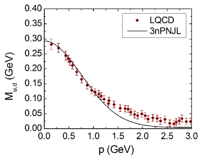
Figure 1: (Color online) Dependence of the dynamical masses of light ($u$ and $d$) quarks on momentum $p$ for the parametrization used in this work. (solid line). The diamond shaped symbols show the results of LQCD calculations for $N_{f}=2+1$ quark flavors extracted from Parappilly et al. (2006).

The form factor $R(p)$, defined in Eq. (II.2) and the given parameters, guarantee a rapid ultra-violet convergence of the loop integrals. As can be seen in Fig. 1, the functional form of the form factor is chosen such that the momentum dependence of the dynamical quark mass is reproduced by the light quarks masses obtained in LQCD calculations Parappilly et al. (2006).

II.3 Spinodal decomposition and the QCD phase diagram

As indicated by extensions of LQCD to finite chemical potentials for finite quark masses Philipsen (2013); Borsanyi et al. (2014); Bellwied et al. (2015), there should be a crossover phase transition in the QCD phase diagram at low chemical potential. In addition, the study of some extrapolations to the continuum limit for $2+1$ quark flavors Bazavov et al. (2012); Aoki et al. (2009); Bazavov et al. (2016) give a critical temperature of around $T_{c}(0)\simeq 155$ MeV.

At large chemical potentials but low temperatures, on the other hand, a first-order phase transition is expected based on phenomenological studies of quark matter (see, for example, Fukushima and Hatsuda (2011), and references therein). This suggests that there should be a second-order phase transition critical end point (CEP) at some critical temperature and critical chemical potential, where the different phase transitions meet. The location of the CEP and the signatures of the first-order phase transition are being investigated in the new experimental facilities as NICA, FAIR and J-PARC, while the intermediate density (crossover) region is the target of the renewed facilities BES and SPS at RHIC and CERN, respectively. These regions are shown in Fig. 2.

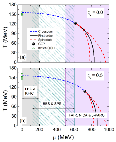
Figure 2: (Color online) Temperature, $T$, versus baryon chemical potential, $\mu$, for 3-flavor quark matter without (a) and with (b) vector interactions. LQCD results Bazavov et al. (2012); Aoki et al. (2009); Bazavov et al. (2016) are marked. The crossover phase transition is shown by the dot-dashed blue line. The dashed red line shows the spinodals, the solid black lines marks the first-order phase transition. The location of the critical endpoint (CEP) is shown by the solid dot.

It is worth noting that according to LQCD simulations at finite temperature and zero chemical potential, chiral symmetry restoration occurs approximately simultaneously with quark deconfinement. The restoration of such symmetry and the consequent melting of the chiral condensate, defined in our model as $\langle\bar{\psi}_{f}\psi_{f}\rangle\,=\,\partial_{m_{f}}\,\Omega$, takes place already in the hadronic phase by parity doubling Aarts et al. (2017), which is signaled by a mass degeneracy of hadronic chiral partner states. A model that restores chiral symmetry in the hadronic phase by lifting the mass splitting between chiral partner states before quark deconfinement sets in has recently been studied in Ref. Marczenko et al. (2018).

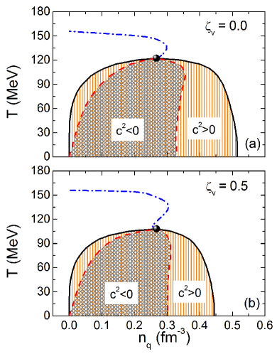
Figure 3: (Color online) Temperature, $T$, versus quark number density, $n_{q}$, for 3-flavor quark matter without (a) and with (b) vector interactions. The crossover and the first order phase transitions are shown by the dot-dashed blue and solid black lines, respectively. The critical endpoint (CEP) is marked with a solid black dot. Unstable ($c_{s}^{2}<0$) and metastable ($c_{s}^{2}>0$) regions are highlighted.

In Figs. 2 and 3 we show the phase diagram of quark matter computed with the 3nPNJL model introduced in Sect. II. The baryon chemical potential is given by $\mu=\sum_{f}\mu_{f}$. In the crossover region (blue dot-dashed line) of Fig. 2, the critical temperatures obtained from LQCD results Bazavov et al. (2012); Aoki et al. (2009); Bazavov et al. (2016) are marked by green triangles. In addition, we have indicated the regions explored by the Beam Energy Scan (BES) of the STAR collaboration at RHIC and by the ALICE Collaboration at the LHC. The first-order phase transition is shown by a black solid line, and the critical endpoint (CEP) is marked with a solid black dot. Finally, the spinodal lines, marked by red dashed lines, show the limit of the metastable regions which will be explained later. It is important to note that the phase diagram shown in Fig. 2 is for quark matter only. This figure, therefore, should not be confused with the full QCD phase diagram. A recent discussion of the QCD phase diagram based on a hadronic model and a chiral quark model (which is simpler than the 3nPNJL model of this work) can be found in Ref. Klähn et al. (2017).

In order to show the effects of vector interaction we have chosen the values $\mathrm{\zeta_{v}}=0.0$ and $\mathrm{\zeta_{v}}=0.5$, the latter being the standard value that follows from the Fierz transformation of the interaction between quark color currents induced by gluon exchange Zhang and Kunihiro (2009).

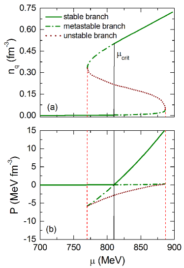
Figure 4: (Color online) (a) Quark number density, $n_{q}$, and (b) pressure, $P$, as a function of baryon chemical potential, $\mu$, at $T=50$ MeV. The dotted, solid and dot-dashed lines show unstable, stable, and metastable equilibrium, respectively.

Using the SU(3) version of the local PNJL model, it has been shown Fukushima (2008b) that the inclusion of repulsive vector interactions among quarks shrinks the first-order transition region by moving the CEP to lower temperatures but higher densities, eventually causing the CEP to vanish at high enough values of the vector coupling constant $\mathrm{\zeta_{v}}$. However, the value chosen for $\mathrm{\zeta_{v}}$ in this work allows for the existence of a CEP, in agreement with the results of LQCD extrapolation techniques Ratti (2018). By comparing panels (a) and (b) in Fig. 2, it can be seen that for the 3nPNJL model used in our work, the inclusion of vector interactions shifts the first-order phase transition to higher chemical potentials and lower temperatures. Finally, the results displayed in panels (a) and (b) in Fig. 3 show that vector interactions tend to shrink the regions (gray areas) where metastable quark matter exists.

The crossover phase transition is determined by the peaks of the chiral susceptibility, as in Contrera et al. (2008); Contrera, G. A. and Orsaria, M. and Scoccola, N. N. (2010). The method of construction of the phase diagram in the ($T,n_{q}$) plane for the first-order phase transition follows from Fig. 4. The dotted lines show unstable equilibrium, solid and dot-dashed lines show stable and metastable equilibria, respectively. The critical first order values ($T_{\rm crit}$, $\mu_{\rm crit}$) used to construct the phase coexistence line in panels (a) and (b) of Fig. 2 are defined by the point where the zig-zag shaped branches of the pressure $P$ cross each other.

The region where density fluctuations associated with the spinodals occurs can be analyzed in term of the isothermal speed of sound, $c_{s}$ given by Randrup, Jørgen (2009, 2010)

$$c_{s}^{2}=\frac{n_{q}}{\epsilon+P}\left(\frac{\partial P}{\partial n_{q}}\right)_{T}\,.$$ (9)

The gray-shaded regions in Fig. 3 show unstable regions in the phase diagram where $c_{s}^{2}<0$. These regions are surrounded by metastable regions shown in orange where $c_{s}^{2}>0$. The dashed red curves show the spinodal lines determined by $c_{s}^{2}=0$, while the blue dot-dashed and the solid black curves show the crossover and first-order phase transitions, respectively.

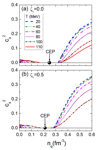
Figure 5: (Color online) Isotherms of the square of the speed of sound, $c_{s}^{2}$, as a function of quark number density, $n_{q}$ without (a), and with (b) vector interactions among quarks. The solid dots indicate the location of the critical endpoints (CEP).

In the region where $c_{s}^{2}<0$, the “compressibility” $\kappa\propto n_{q}(\frac{\partial P}{\partial n_{q}})_{T}$ Schmitt (2010)) is negative and the system responds to an increase in density by enlarging any small density fluctuations. Since this region is not stable, all the density fluctuations that normally occur in the zone bounded by the isothermal spinodals will separate the system into regions of low density and high density. The spinodal curves separate unstable regions from metastable regions in Fig. 3. The right branch of the spinodal curve shows the regions where an increase in density in the denser phase does not cause any change in pressure. The left branch of the spinodal shows the equivalent to this, but for the less dense phase. The metastable region is bounded by the coexistence region and the isothermal spinodal curve. It is in this region where density fluctuations either grow through the aggregation of quark condensates (left branch) or shrink because of the evaporation of these condensates (right branch). It is worth noticing that if one wants to construct an equation of state for deconfined quark matter, it is necessary to work with chemical potentials that lie on the right-hand side of the spinodal lines so that perturbations do not lead to the formation of mesons.

The behavior of $c_{s}^{2}$ (in units of the speed of light) as a function of quark number density is shown in Fig. 5 for different temperatures. Note that for the cases without vector interactions $c_{s}^{2}$ is less than $1/3$, as suggested for weakly interacting quark matter Bedaque and Steiner (2015). Non-vanishing vector interactions among quarks stiffen the EoS and the speed of sound increases to values greater than $1/3$. (The region where $c_{s}^{2}<0$, which correspond to the unstable region of the first-order phase transitions, has been omitted in Fig. 5.)

III Hadronic matter at finite temperature

In the most primitive conception, the matter in the core of a neutron star is constituted from neutrons. At a slightly more accurate representation, the cores consist of neutrons and protons whose electric charge is balanced by leptons ($L=\{e^{-},\mu^{-}\}$). Other particles, like hyperons ($B=\{n,p,\Lambda,\Sigma,\Xi\}$) and the $\Delta$-isobar, may be present if the Fermi energies of these particles become large enough so that the existing baryon populations can be rearranged and a lower energy state be reached. To model this hadronic phase, we make use of the density-dependent relativistic mean-field (DDRMF) theory, in which the interactions between baryons are described by the exchange of scalar ($\sigma$), vector ($\omega$), and isovector ($\rho$) mesons. The lagrangian of this model is given by

$$\mathcal{L} = \sum_{B}\bar{\psi}_{B}\bigl{[}\gamma_{\mu}[i\partial^{\mu}-g_{\omega B}(n)\omega^{\mu}-g_{\rho B}(n){\boldsymbol{\tau}}\cdot{\boldsymbol{\rho}}^{\mu}]$$

$$- [m_{B}-g_{\sigma B}(n)\sigma]\bigr{]}\psi_{B}+\frac{1}{2}(\partial_{\mu}\sigma\partial^{\mu}\sigma-m_{\sigma}^{2}\sigma^{2})$$

$$- \frac{1}{3}\tilde{b}_{\sigma}m_{N}[g_{\sigma N}(n)\sigma]^{3}-\frac{1}{4}\tilde{c}_{\sigma}[g_{\sigma N}(n)\sigma]^{4}-\frac{1}{4}\omega_{\mu\nu}\omega^{\mu\nu}$$

$$+ \frac{1}{2}m_{\omega}^{2}\omega_{\mu}\omega^{\mu}+\frac{1}{2}m_{\rho}^{2}{\boldsymbol{\rho\,}}_{\mu}\cdot{\boldsymbol{\rho\,}}^{\mu}-\frac{1}{4}{\boldsymbol{\rho\,}}_{\mu\nu}\cdot{\boldsymbol{\rho\,}}^{\mu\nu}\,,$$

where $g_{\sigma B}(n)$, $g_{\omega B}(n)$ and $g_{\rho B}(n)$ are density dependent meson-baryon coupling constants and $n=\sum_{B}n_{B}$ is the total baryon number density. The density dependent coupling constants are given by Typel (2018)

$$g_{iB}(n)=g_{iB}(n_{0})\,\,a_{i}\,\frac{1+b_{i}(\frac{n}{n_{0}}+d_{i})^{2}}{1+c_{i}(\frac{n}{n_{0}}+d_{i})^{2}}\,,$$ (11)

for $i=\sigma,\omega$ and

$$g_{\rho B}(n)=g_{\rho B}(n_{0})\,\mathrm{exp}\left[\,-a_{\rho}\left(\frac{n}{n_{0}}-1\right)\,\right]\,.$$ (12)

This choice of parametrization accounts for nuclear medium effects Fuchs et al. (1995). The parameters $a_{i}$, $b_{i}$, $c_{i}$, and $d_{i}$ are fixed by the binding energies, charge and diffraction radii, spin-orbit splittings, and the neutron skin thickness of finite nuclei. Note that the density dependence of the meson-baryon couplings in the DD2 parametrization eliminates the need for non-linear self-interactions of the $\sigma$ meson. Therefore, the non-linear terms in the lagrangian given in Eq. (III) are considered only for the GM1L parametrization.

The meson-hyperon coupling constants have been determined following the Nijmegen extended soft core (ESC08) model Rijken et al. (2010). The relative isovector meson-hyperon coupling constants were scaled with the hyperon isospin and for the $\Delta$-isobar $x_{{\sigma}{\Delta}}=x_{{\omega}{\Delta}}=1.1$ and $x_{{\rho}{\Delta}}=1.0$, where $x_{iH}=g_{iH}/g_{iN}$ was used (see Spinella (2017) for details).

In Table 1 we list the parameters of the DDRMF models used in this work. Table 2 shows the saturation properties of the models, which are the nuclear saturation density, $n_{0}$, energy per nucleon, $E_{0}$, nuclear incompressibility, $K_{0}$, effective nucleon mass, $m^{*}/m_{N}$, asymmetry energy, $J$, slope of the asymmetry energy, $L_{0}$, and the nucleon potential, $U_{N}$.

Parameters	GM1L	DD2
$m_{\sigma}$ (GeV)	0.5500	0.5462
$m_{\omega}$ (GeV)	0.7830	0.7830
$m_{\rho}$ (GeV)	0.7700	0.7630
$g_{\sigma N}$	9.5722	10.6870
$g_{\omega N}$	10.6180	13.3420
$g_{\rho N}$	8.9830	3.6269
$\tilde{b}_{\sigma}$	0.0029	0
$\tilde{c}_{\sigma}$	$-0.0011$	0
$a_{\sigma}$	0	1.3576
$b_{\sigma}$	0	0.6344
$c_{\sigma}$	0	1.0054
$d_{\sigma}$	0	0.5758
$a_{\omega}$	0	1.3697
$b_{\omega}$	0	0.4965
$c_{\omega}$	0	0.8177
$d_{\omega}$	0	0.6384
$a_{\rho}$	0.3898	0.5189

Table 1: Parameters of the DDRMF parametrizations that lead to the properties of symmetric nuclear matter at saturation density given in Table 2.

Saturation Properties	GM1L	DD2
$n_{0}$ (fm-3)	0.153	0.149
$E_{0}$ (MeV)	$-16.30$	$-16.02$
$K_{0}$ (MeV)	300.0	242.7
$m^{*}/m_{N}$	0.70	0.56
$J$ (MeV)	32.5	32.8
$L_{0}$ (MeV)	55.0	55.3
$-U_{N}$ (MeV)	65.5	75.2

Table 2: Properties of nuclear matter at saturation density computed for the DDRMF parametrizations GM1L Spinella (2017); Spinella et al. (2018) and DD2 Typel et al. (2010).

The meson mean-field equations following from Eq. (III) are given by

$$m_{\sigma}^{2}\bar{\sigma} = \sum_{B}g_{\sigma B}(n)n_{B}^{s}-\tilde{b}_{\sigma}\,m_{N}\,g_{\sigma N}(n)(g_{\sigma N}(n)\bar{\sigma})^{2}$$

$$-\tilde{c}_{\sigma}\,g_{\sigma N}(n)\,(g_{\sigma N}(n)\bar{\sigma})^{3}\,,$$

$$m_{\omega}^{2}\bar{\omega} = \sum_{B}g_{\omega B}(n)n_{B}\,,$$ (13)

$$m_{\rho}^{2}\bar{\rho} = \sum_{B}g_{\rho B}(n)I_{3B}n_{B}\,,$$

where $I_{3B}$ is the 3-component of isospin and $n_{B}^{s}$ and $n_{B}$ are the scalar and particle number densities for each baryon $B$, which are given by

$$n_{B}^{s} = \gamma_{B}\int\frac{d^{3}p}{(2\pi)^{3}}\left[f_{B-}(p)-f_{B+}(p)\right]\frac{m_{B}^{*}}{E_{B}^{*}},$$ (14)

$$n_{B} = \gamma_{B}\int\frac{d^{3}p}{(2\pi)^{3}}\left[f_{B-}(p)-f_{B+}(p)\right]\,.$$ (15)

Here $f_{B\mp}$ denotes the Fermi-Dirac distribution function and $E^{*}_{B}$ stands for the effective baryon energy given by

$$f_{B\mp}(p)=\frac{1}{\exp\left[\frac{E_{B}^{*}(p)\mp\mu_{B}^{*}}{T}\right]+1},\,\,\,\,E_{B}^{*}(p)=\sqrt{p^{2}+m_{B}^{*2}}\,,$$

where $\gamma_{B}=2J_{B}+1$ is the spin degeneration factor and $m_{B}^{*}=m_{B}-g_{\sigma B}(n)\bar{\sigma}$ is the effective baryon mass. We shall note at this point, that this model does not distinguish from parity in mass eigenstates. Because of that, the neutron mass is set to $m_{N}=939.6$ MeV and that is the value that it takes when the background $\sigma$ field goes to zero. For a detailed explanation of a model that distinguish hadronic chiral partner states see Marczenko and Sasaki (2018). The effective chemical potential, $\mu_{B}^{*}$, is given by

$$\mu_{B}^{*}=\mu_{B}-g_{\omega B}(n)\bar{\omega}-g_{\rho B}(n)\bar{\rho}I_{3B}-\widetilde{R}\,,$$ (16)

where $\widetilde{R}$ is the rearrangement term given by

$$\widetilde{R}=\sum_{B} \left(\frac{\partial g_{\omega B}(n)}{\partial n}n_{B}\bar{\omega}+\frac{\partial g_{\rho B}(n)}{\partial n}I_{3B}n_{B}\bar{\rho}\right.$$

$$- \left.\frac{\partial g_{\sigma B}(n)}{\partial n}n_{B}^{s}\bar{\sigma}\right)\,,$$

which is important for achieving thermodynamical consistency Hofmann et al. (2001). This term also contributes to the total baryonic pressure of the matter,

$$P = \sum_{B}\frac{\gamma_{B}}{3}\int\frac{d^{3}p}{(2\pi)^{3}}\frac{p^{2}}{E_{B}^{*}}[f_{B-}(p)+f_{B+}(p)]$$

$$- \frac{1}{2}m_{\sigma}^{2}\bar{\sigma}^{2}+\frac{1}{2}m_{\omega}^{2}\bar{\omega}^{2}+\frac{1}{2}m_{\rho}^{2}\bar{\rho}^{2}$$

$$- \frac{1}{3}\tilde{b}_{\sigma}m_{N}(g_{\sigma N}(n)\bar{\sigma})^{3}-\frac{1}{4}\tilde{c}_{\sigma}(g_{\sigma N}(n)\bar{\sigma})^{4}+n\widetilde{R}.$$

The expression for the energy density, $\epsilon$, is determined by the Gibbs relation given in Eq. (27).

IV Neutron star matter and neutron stars

For the description of the matter inside of (proto-) neutron stars, leptons must be also taken into account in both, the hadronic and the quark matter models. They can be treated as free Fermi gases with the grand canonical potential given by

$$\Omega_{L}=-\sum_{L}\frac{\gamma_{L}}{3}\int\frac{d^{3}p}{(2\pi)^{3}}\frac{p^{2}}{E_{L}}[f_{L-}(p)+f_{L+}(p)]\,,$$ (19)

with the lepton distribution function given by

$$f_{L\mp}(p) = \frac{1}{\exp\left[\frac{E_{L}(p)\mp\mu_{L}}{T}\right]+1},\,\,\,\,\,\,E_{L}(p)=\sqrt{p^{2}+m_{L}^{2}}\,.$$

The lepton degeneracy factor is given by $\gamma_{L}=2$. The sum over $L$ in Eq. (19) runs over $e^{-}$ and $\mu^{-}$ with masses $m_{L}$ and, when correspond (see Sect. V.3), massless neutrinos, $\nu_{e}$.

In addition, the composition of the matter in a neutron star is constrained by charge neutrality and $\beta-$equilibrium. Electric charge and baryon number are conserved. The conditions of electric charge neutrality and of baryon number conservation lead to

$$\sum_{B}q_{B}\,n_{B}+\sum_{L}q_{L}\,n_{L}=0\,,$$ (20)

and

$$\sum_{B}\,n_{B}-n=0\,,$$ (21)

where the subscripts $B$ and $L$ stand for baryons and leptons respectively, $q_{i}$ is the electric charge of these particles.

The condition of chemical equilibrium reads

$$\mu_{B}=\mu_{n}-q_{B}(\mu_{e}-\mu_{\nu_{e}})\,,$$ (22)

where $\mu_{n}$, $\mu_{e}$ and $\mu_{\nu_{e}}$ are the neutron, electron and neutrino chemical potentials, respectively. For the quark matter phase, this condition is given by

$$\mu_{f}=\widetilde{\mu}-q_{f}(\mu_{e}-\mu_{\nu_{e}})\,,$$ (23)

where $\mu_{n}$ is replaced by an average quark chemical potential $\widetilde{\mu}=(\mu_{u}+\mu_{d}+\mu_{s})/3$, which facilitates the numerical calculations, and $q_{f}$ represent the electric charge of each quark flavor.

The lepton chemical potential follows from the equilibrium reaction

$$e^{-}\leftrightarrow\mu^{-}+\nu_{e}+\bar{\nu}_{\mu}\,,$$ (24)

which leads to

$$\mu_{e}=\mu_{\mu}+\mu_{\nu_{e}}+\mu_{\bar{\nu}_{\mu}}\,.$$ (25)

Neutrinos are trapped in the very early stages of the life of a proto-neutron star, during which it is assumed that the lepton fraction is kept constant. This can be expressed mathematically as

$$Y_{Le}=\frac{n_{e}+n_{\nu_{e}}}{n}=\xi,$$

$$Y_{L\mu}=\frac{n_{\mu}+n_{\nu_{\mu}}}{n}=0\,.$$ (26)

During this phase, the stellar matter is opaque to neutrinos and its composition is characterized by three independent chemical potentials, which are $\mu_{n}$, $\mu_{e}$, and $\mu_{\nu_{e}}$. The condition $Y_{L\mu}=0$ accounts for the fact that no muons are present in the matter when neutrinos are trapped. The value of $\xi\simeq 0.4$ depends on the efficiency of electron capture reactions during the initial state of the formation of proto-neutron stars Prakash et al. (1997).

When the star cools down, the stellar matter becomes transparent to neutrinos so that $\mu_{\nu_{e}}=\mu_{\bar{\nu}_{\mu}}=0$. In this case the number of independent chemical potentials is reduced from three to two, $\mu_{n}$ and $\mu_{e}$.

IV.1 Dense matter phase transition and hybrid EoS

To model the phase equilibrium between hadronic matter and quark matter, we shall assume that this equilibrium is of first order and Maxwell-like, that is, the pressure in the mixed quark-hadron phase is constant. Theoretically the transitions could be Gibbs-like as well, depending on the surface tension at the hadron-quark interface. The value of the surface tension is only poorly known. Lattice gauge calculations, for instance, predict surface tension values in the range of $0-100$ MeV fm^-2 Kajantie et al. (1991). According to theoretical studies, surface tensions above around $70$ MeV fm^-2 favor the occurrence of a sharp (Maxwell-like) quark-hadron phase transition rather than a softer Gibbs-like transition Sotani et al. (2011); Yasutake et al. (2014). In this paper, we consider a sharp Maxwell-like transition.

Given the theoretical models for quark matter and hadronic matter discussed in Sects. II and III, we now proceed to construct models for the hybrid EoS of compact stars. The EoS for both the hadronic phase and the quark phase is given by the Gibbs relation

$$\epsilon=-P+TS+\sum_{i}\mu_{i}\,n_{i}\,,$$ (27)

where $P=-\Omega$, $S=\frac{\partial P}{\partial T}$ and $n_{i}=\frac{\partial P}{\partial\mu_{i}}$ ($i$ stands for all the particles of each phase, including leptons). The lepton contributions to $P$ and $S$ follow from $\Omega_{L}$ given by Eq. (19).

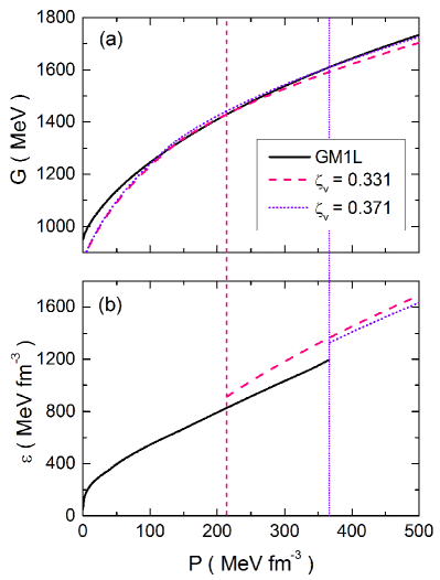
Figure 6: (Color online) Panel (a) shows the construction of the EoS (at $T=0$) from the Gibbs free energy (per particle), $G$, for the hybrid GM1L-3nPNJL parametrization. The solid black line represents the hadronic (GM1L) EoS and the red dashed and blue dotted lines are the EoSs of the quark (3nPNJL) phase for two values of the vector coupling constant, $\mathrm{\zeta_{v}}$. Panel (b) shows the energy density, $\epsilon$, as function of pressure, $P$, for the two values of $\mathrm{\zeta_{v}}$, discussed in the text.

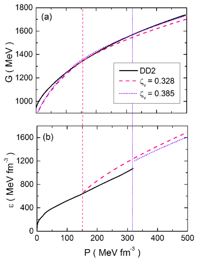
Figure 7: (Color online) Panel (a) shows the construction of the EoS (at $T=0$) from the Gibbs free energy (per baryon) $G$ for hybrid DD2-3nPNJL parametrization. The solid black line represents the hadronic (DD2) EoS and the red dashed and blue dotted lines are the EoSs for the quark (3nPNJL) phase for two values of the vector coupling constant, $\mathrm{\zeta_{v}}$. Panel (b) shows the energy density, $\epsilon$, as function of pressure, $P$, for the two values of $\mathrm{\zeta_{v}}$, discussed in the text.

To construct the hadron-quark phase transition we adopt the Gibbs condition, i.e., the phase transition between both phases occurs when

$$G_{H}(P,T)=G_{Q}(P,T)\,,$$ (28)

where $G_{H}$ respectively $G_{Q}$ are the Gibbs free energy per baryon for the hadronic ($H$) and quark ($Q$) phases at a given pressure and transition temperature. The Gibbs energy of each phase ($i=H,Q$) is given by

$$G_{i}(P,T)=\sum_{j}\frac{n_{j}}{n}\mu_{j}\,,$$ (29)

where the sum over $j$ is over all the particles present in each phase. It is important to remark that this is the correct treatment to calculate a phase transition when different particle species are present in both phases. In the case of Fig. 4, one is allowed to use both the Gibbs free energy or the chemical potential to model the phase transition, since there are quarks in both phases. In contrast, for the hadron-quark phase transition, the particle chemical potentials in each phase are different so that is becomes necessary to calculate the Gibbs free energy as a function of pressure to construct the phase transition Hempel et al. (2013), as done in Figs. 6 and 7 for the GM1L and DD2 parameterizations, respectively. In these figures, two transitions are visible, the first one from quark to hadronic matter at pressures $P\sim 100-150$ MeV/fm³, and the second one from hadronic to quark matter at $P\sim 350-400$   MeV/fm³. The hadronic and the quark matter EoS are very similar and this makes it difficult to distinguish between the two phases in the range of the relevant pressures, $P\sim 100-400$ MeV/fm³. This can be interpreted as a masquerade behavior of dense matter, different from pure deconfined quark matter Alford et al. (2005).

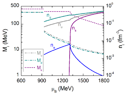
Figure 8: (Color online) Dynamical masses, $M_{i}$, and number densities, $n_{i}$, of up, down and strange quarks as a function of baryon chemical potential. $n_{e}$ denotes the number density of electrons.

It can be seen from Fig. 8 that a first order phase transition occurs at a baryonic chemical potential of $\mu_{B}\sim$ 940 MeV, indicated by the discontinuities in the particle number densities and the dynamic quark masses. For baryon chemical potentials between 940 MeV and 1300 MeV we have a phase where the chiral quark condensate of the up and down quarks, $\langle\bar{u}\,u\rangle\,=\,\langle\bar{d}\,d\rangle\,\sim\,0$, while $\langle\bar{s}\,s\rangle\neq 0$. Such phase exhibits a structure similar to hadronic matter and the first quark phase-to-hadron transition is unphysical with condensed strange quasi-particles states (the first crossing of hadronic and quarks matter curves in Figs. 6 and 7). This behavior could indicate the existence of a phase which has both aspects of nuclear and quark matter (see McLerran and Pisarski (2007); Baym et al. (2018), and references therein). Beyond $\mu_{B}$ $\sim 1300$ MeV and P $\sim 135$ $\mathrm{MeV/fm^{3}}$, the strange quarks suffer a crossover transition and then deconfine, becoming part of the deconfined quark phase used to construct the hybrid EoS. In this regime up and down quarks could form diquarks and condense in a color superconducting state, provided the value of the diquark coupling is sufficiently large Blaschke et al. (2009).

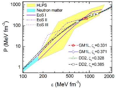
Figure 9: (Color online) Comparison of the zero-temperature quark-hybrid EoSs of this work (GM1L, DD2) with models (HLPS, Neutron EoS I, EoS II, EoS III) from the literature Krüger et al. (2013); Hebeler et al. (2013); Kurkela et al. (2014). The solid dots mark the beginning and the end of the quark-hadron phase for our EoSs. The symbol $\mathrm{\zeta_{v}}$ denotes the vector interaction strengths.

The crossing of the Gibbs energy of the two phases in the $G-P$ plane defines the phase transition point for a given transition temperature, $T_{\textrm{{trans}}}$. The $2\,M_{\odot}$ constraint of PSR J1614-2230 and PSR J0348+0432 Demorest et al. (2010); Lynch et al. (2013); Antoniadis et al. (2013); Arzoumanian et al. (2018) and the assumption that quark matter exists in the cores of neutron stars have been used to determine the range of the vector coupling constant $\mathrm{\zeta_{v}}$ in the quark matter. This leads to $0.331<\mathrm{\zeta_{v}}<0.371$ for GM1L, and $0.328<\mathrm{\zeta_{v}}<0.385$ for DD2, where the lower bounds are determined by the $2\,M_{\odot}$ constraint and the upper bounds by the existence of quark matter in the cores of neutron stars. It is worth noticing that the density range covered by the 3nPNJL model is such that the spinodal region (and hence the possible hadronization of deconfined quark matter) is not encountered.

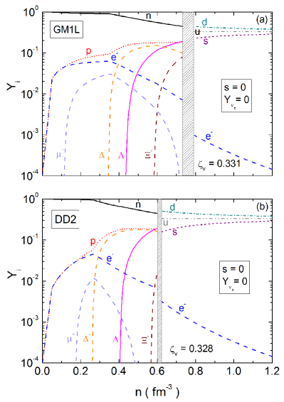
Figure 10: (Color online) Particle population of stellar quark-hybrid matter at zero temperature as a function of baryonic number density. The populations are computed for GM1L-3nPNJL and DD2-3nPNJL (see text). $\mathrm{\zeta_{v}}$ denotes the strength of the vector repulson among quarks.

The quark-hybrid EoSs GM1L-3nPNJL and DD2-3nPNJL computed at zero temperature are compared in Fig. 9 with nuclear EoSs suggested in the literature. The curves labeled EoS I, EoS II, and EoS III are the EoSs determined by Kurkela et al. Kurkela et al. (2014), which are based on an interpolation between the regimes of low-energy chiral effective field theory and high-density perturbative QCD. The region labeled HLPS has been established by Hebeler, Lattimer, Pethick, and Schwenk, and the area labeled ‘Neutron matter’ shows the equation of state of low-density neutron matter Krüger et al. (2013); Hebeler et al. (2013). It can be seen that the super-dense portions of the hybrid EoSs obtained in our work are well within these limits.

In Fig. 10, we shown the quark-hadron compositions of cold neutron stars computed for GM1L-3nPNJL and DD2-3nPNJL. As expected, the diversity of particles is significantly reduced at $T=0$. Even though, the $\Delta^{-}$-isobar still plays an important role in our calculations as it reduces the lepton population notably. As can also be seen, the only strangeness-carrying hyperons that contribute to the composition are the $\Lambda$’s and the $\Xi^{-}$’s, in sharp contrast to the finite $T$ case (Figs. 14 and 15). A comparison of the GM1L and DD2 populations shows that the particle abundances are qualitatively similar to each other, and the threshold densities of the individual particles species are only shifted modestly.

IV.2 Properties of static equilibrium configurations

To determine the mass-radius relationship for (proto-) neutron stars we solve the Tolman-Oppenheimer-Volkoff (TOV) equation Tolman (1939) given by

$$\frac{dP}{dr}=-\frac{m(r)\epsilon(r)}{r^{2}}\frac{[1+P(r)/\epsilon(r)][1+4\pi r^{3}P(r)/m(r)]}{1-2m(r)/r}\,,$$ (30)

where $P(r)$ and $\epsilon(r)$ are the pressure and energy density at a radial distance $r$ from the star’s center. The gravitational mass follows from integrating

$$\frac{dm}{dr}=4\pi r^{2}\,\epsilon(r)\,.$$ (31)

from $r=0$ to the star’s radius, $R$. The latter is defined by $P(R)=0$. The star’s total gravitational mass is thus given by

$$M_{G}\equiv 4\,\pi\int_{0}^{R}r^{2}\epsilon(r)dr\,.$$ (32)

In Sect. V.3 we will discuss stages in the evolution of proto-neutron stars to neutron star in the gravitational-mass versus baryon-mass diagram. The latter is given by

$$M_{B}=m_{n}\int_{0}^{R}\frac{4\pi r^{2}n(r)}{[1-2Gm(r)/r]^{1/2}}dr\,,$$ (33)

where $m_{n}=939$ MeV is the nucleon mass.

We first perform the calculations at zero temperature. The results will be compared with the finite temperature and neutrino trapped results in Sect. V. Fig.  11 shows the gravitational mass as a function of central energy density as well as a function of stellar radius for the minimum vector interaction coupling constants of each hadronic parametrization. The properties of the maximum-mass stars are summarized in Table 3.

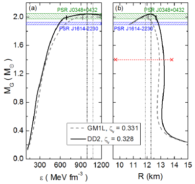
Figure 11: (Color online)(a) Gravitational mass as a function of central energy density, and (b) gravitational mass as a function of stellar radius, for $T=0$ MeV. The vertical bars show the onset of the transition of hadronic matter to quark matter. The vertical dash-dotted lines mark the location of the maximum-mass star for each EoS. The dashed horizontal line shows the estimate of a $1.40M_{\odot}$ neutron-star radius derived from GW170817 Bauswein et al. (2017); Fattoyev et al. (2018); Raithel et al. (2018a); Most et al. (2018a); Annala et al. (2018).

As can be seen, both the pure hadronic EoS as well as the hybrid Eos lead to maximum-mass neutron stars with fulfill the $2M_{\odot}$ mass constraint. We also note that the DD2 neutron stars contain a wider branch of quark-hybrid stars than the GM1L stars, since the DD2 EoS is stiffer in terms of the Gibbs free energy so that the hadron-quark phase transition occurs at a lower pressure.

Color superconductivity (CSC) has not been taken into account in this work since a number of problems (such as the diagonalization of the Polyakov loop in color space) need to be overcome first. However, based on the works carried out in Ref. Ruester et al. (2005) for a local three-flavor model and in Ref. Alvarez-Castillo et al. (2019) for a non-local two flavor model, one could expect that incorporating CSC into our model will shift the onset of the hadron-quark phase transition to lower densities, provided, of course, the results of Ruester et al. (2005); Alvarez-Castillo et al. (2019) have their quantitative correspondence in the theoretical model studied in this paper. If so, this would somewhat increase the amount of quark matter in the cold neutron stars of our paper. Their maximum masses, however, will not be impacted much since they are almost exclusively determined by the hadronic parts of the equations of state. The situation is much harder to assess for CSC quark matter at finite temperature (entropy) for conditions prevailing in the cores of proto-neutron stars. Chiefly among the open issues is the actual size of the gap(s) in the CSC phase which, for a given condensation pattern, depend on the density and the critical temperature of the CSC phase. Any in-depth calculation attempting to address this issue is hampered by the fact that the gap(s) is (are) to be computed for quark matter constrained by the conditions of color neutrality, electric charge neutrality, and chemical equilibrium Blaschke et al. (2005).

$\mathrm{GM1L}$
	$M_{G}~{}[M_{\odot}]$	$M_{B}~{}[M_{\odot}]$	$\epsilon_{c}~{}[\mathrm{MeV/fm^{3}}]$
$\mathrm{Pure\,\,hadronic}$	$2.04$	$2.42$	$1194.82$
$\mathrm{\zeta_{v}}=0.331$	$2.00$	$2.36$	$1077.02$
$\mathrm{\zeta_{v}}=0.371$	$2.04$	$2.42$	$1295.79$
$\mathrm{DD2}$
	$M_{G}~{}[M_{\odot}]$	$M_{B}~{}[M_{\odot}]$	$\epsilon_{c}~{}[\mathrm{MeV/fm^{3}}]$
$\mathrm{Pure\,\,hadronic}$	$2.11$	$2.53$	$1110.68$
$\mathrm{\zeta_{v}}=0.328$	$2.04$	$2.43$	$992.88$
$\mathrm{\zeta_{v}}=0.385$	$2.11$	$2.54$	$1194.82$

Table 3: Gravitational mass, $M_{G}$, and baryon mass, $M_{B}$, of the maximum-mass neutron stars (zero temperature) computed for GM1L and DD2. The quantity $\epsilon_{c}$ denotes the stars’ cental density.

Figure 12: (Color online). Energy density as a function of radius for the maximum-mass neutron stars shown in Fig. 11. The density discontinuities at around 2 and 3.5 km (dash-dotted vertical lines) are caused by the quark-hadron phase transition in these stars.

In Fig. 12 we present energy density profiles for the maximum-mass stars shown in Fig. 11. As can be seen, these stars contain quark matter cores that are several kilometers in size, i.e., $R_{\rm core}\sim 3.5$ km for the DD2 parameter set and $R_{\rm core}\sim 2$ km for the GM1L.

V Application to proto-neutron stars

V.1 Finite temperatures and mass-radius relationship

To study proto-neutron stars we need to extend the EoSs of this work to finite temperatures. It is known from previous works (see, for example, Pons et al. (1999)) that proto-neutron stars are nearly isentropic and not isothermal. To obtain an isentropic hybrid EoS for the Maxwell construction, we first compute the hadronic and the quark EoS for a given transition temperature (i.e., 15 and 30 MeV). Upon determining the crossing point of these EoSs in the $G-P$ plane, we then determine the isentropic hybrid EoS for that transition temperature.

As already mentioned before, neutrinos play an important role for the composition of newly formed, hot proto-neutron stars. For example, it has been shown in Ref. Pons et al. (1999) that during the deleptonization phase, the stellar core of a proto-neutron star is heated by neutrino transport (Joule heating), and that the maximum heating occurs just before the neutrinos escape from the star. The maximum temperature reached at this evolutionary stage is around $T\simeq 40-45$ MeV. As a result, different lepton and neutrino fractions at given entropy values are to be considered when studying different stages in the evolution of proto-neutron stars to neutron stars. This will be done in section V.3 below.

We begin this section by studying the effects of temperature on the properties of hot stars. For this purpose we have constructed isentropic EoSs for the parameterizations of this work, choosing representative proto-neutron star temperatures of $T=15$ and $30$ MeV. Depending on the star’s evolutionary stage, the presence of neutrinos is taken into account too (i.e., $Y_{\nu_{e}}\neq 0$), and the lepton fractions that we consider are $Y_{L}=Y_{e}+Y_{\nu_{e}}=0.2$ or 0.4. The mass radius relationships of stars made up of such matter are shown in Fig. 13.

For the maximum values of the vector interaction for each hadronic parametrization ($\mathrm{\zeta_{v}}=0.371$ and $\mathrm{\zeta_{v}}=0.385$) we found that an increase in temperature (with and without neutrinos) opposes the formation of quark matter in the cores of stars. The only stars found to contain quark matter (for these $\mathrm{\zeta_{v}}$ values) are the zero-temperature neutron stars. For the minimum values of the vector interaction the results are qualitatively similar to the maximum-value case. Differences concern primarily the trapping of neutrinos. For the DD2 parametrization, for instance, a hybrid EoSs with trapped neutrinos can be constructed up to $T_{\textrm{{trans}}}=30$ MeV (labeled as ${\rm T_{30}}$ in Fig. 13). For the GM1L parametrization, however, neutrinos are only present in the matter up to $T_{\textrm{{trans}}}=15$ MeV (${\rm T_{15}}$, for higher transition temperatures, the stars become unstable before the phase transition occurs).

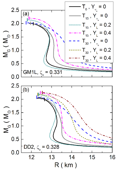
Figure 13: (Color online) Gravitational mass, $M_{G}$, as a function of radius, $R$, for quark-hybrid stars at different transition temperatures, $T_{\textrm{{trans}}}$, of the quark-hadron phase transition. $Y_{L}$ denotes the lepton fraction and $Y_{\nu_{e}}$ the neutrino fraction. The vertical bars mark the onset of quark deconfinement. With the exception of the neutrino-less ($Y_{\nu_{e}}=0$) stars with $T_{\rm trans}=0$ (${\rm T_{0}}$) and $T_{\rm trans}=15$ MeV (${\rm T_{15}}$), this transition happens at the maximum-mass peak.

As expected, in Fig. 13 it can be observed that the influence of neutrino trapping in the maximum mass stars is greater than those originated from a fixed entropy per baryon. As shown for example in Ref. Prakash et al. (1997), such influence depends sensibly on the matter composition, in particular, if heavy hadrons (like hyperons and $\Delta$-isobars) and quarks are taken into account. This behavior is in sharp contrast to the idealized EoS containing only nucleons and leptons and no additional softening components, where neutrino trapping generally reduce the maximum mass.

V.2 Dense proto-neutron star matter

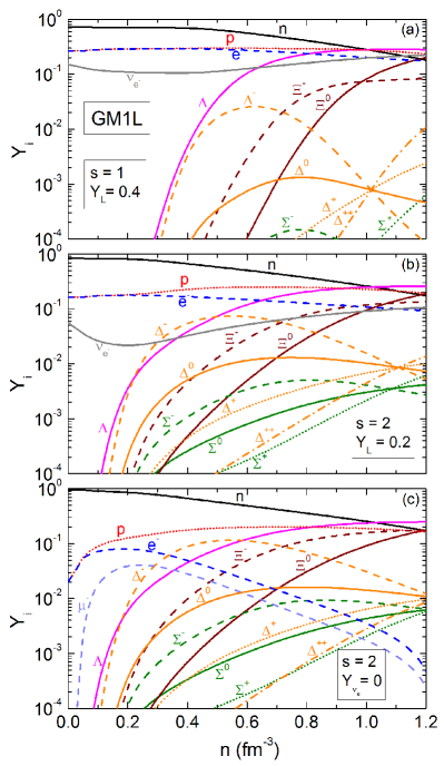
Figure 14: (Color online) Particle populations of proto-neutron star matter for the GM1L parametrization. The compositions correspond to matter in the cores of proto-neutron stars at different evolutionary stages characterized by entropy per baryon, $s$, and lepton number, $Y_{L}$.

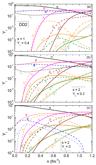
Figure 15: (Color online) Same as Fig. 14, but for the DD2 parametrization.

Figs. 14 and 15 show the particle populations of proto-neutron star matter computed for the hadronic parametrizations used in this work. It can be seen that the particle populations depend sensitively on entropy per baryon, $s=S/n$, and lepton number, $Y_{L}$. This is particularly the case for the $\Delta$-isobar. The negatively charged state of this particle are populated first, replacing some of the high-energy electrons. The other three stages of the $\Delta$-isobar (i.e., $\Delta^{0}$, $\Delta^{+}$, and $\Delta^{++}$) are successively populated at densities that are just a few times greater than the nuclear saturation density. All these stages therefore exist in the cores of proto-neutron stars, according to our model. Another striking difference concerns the high abundance of electrons in matter where the lepton fraction is non-zero and neutrinos are present (top (a) and middle (b) panels of Figs. 14 and 15). Because of that, one may speculate that the electric conductivity of such matter is considerably different from the electric conductivity of neutrino-free stellar matter (bottom (c) panels of Figs. 14 and 15), where the presence of muons leads to fewer electrons in the system, and the increasing $\Delta^{-}$, $\Xi^{-}$, and $\Sigma^{-}$ populations cause a further reduction of the number of leptons. Regarding the strangeness-carrying hyperons, their main contributions come from the $\Lambda$’s and $\Xi$’s, whose populations grow monotonically with density, dominating the stellar matter composition at very high densities. Other hyperons species are also present, but to a lesser degree.

V.3 Stages in the evolution of proto-neutron stars to neutron stars

In this section, we use the EoSs of this paper to study several stages in the evolution of proto-neutron stars to neutron stars Prakash et al. (1997). Shortly after core bounce a proto-neutron star is hot and lepton rich. The entropy per baryon and lepton fraction of the matter in the core of such an object change quickly from around $s=1$ and $Y_{L}=0.4$ to $s=2$ and $Y_{L}=0.2$. Subsequent core heating and deleptonization change these values to $s=2$ and $Y_{\nu_{e}}=0$, leading to a hot lepton-poor neutron star in less than a minute after the star’s birth Pons et al. (1999). After several minutes this hot neutron star has cooled down to temperatures less than 1 MeV, that is, the star has become cold. From then on, the star continues to slowly cool via neutrino and photon emission until the thermal radiation becomes too weak to be detectable with x-ray telescopes.

In Fig. 16, we show the gravitational-mass versus baryon-mass relationship of stars with entropies and lepton numbers that correspond to the different stages in the evolution of proto-neutron stars to neutron stars described just above. Assuming we are working with isolated stars, the baryonic mass should be a conserved quantity along the different stages of stellar evolution. As an example, this condition is represented by a vertical dashed line passing through the maximum mass cold star in Fig. 16. The short vertical bars in this figure mark the onset of quark deconfinement in the cores of these stars. Proto-neutron stars in their earliest stages of evolution (i.e., $s=1$, $Y_{L}=0.4$ and $s=2$, $Y_{L}=0.2$) are found to be made of pure hadronic matter, no matter how massive. Once these stars have deleptonized ($Y_{\nu_{e}}=0$) and their core entropies have dropped to entropies of $s=1.5$ and 0.8, the density at quark deconfinement sets in is reached. But this turns out, for our sample stars, to happen only in stars that are in the gravitationally unstable region (shaded areas in Fig. 16), where the proto-neutron stars have greater baryonic mass than the corresponding maximum mass cold star. The situation is different once the temperature has dropped to just a few MeV, that is, when these stars have turned into cold ($s=0$, $Y_{\nu_{e}}=0$) neutron stars, which possess pure quark matter in their cores. In Tables 4 and 5 we show the changing core compositions of proto-neutron stars as they evolve to the associated maximum-mass cold stars.

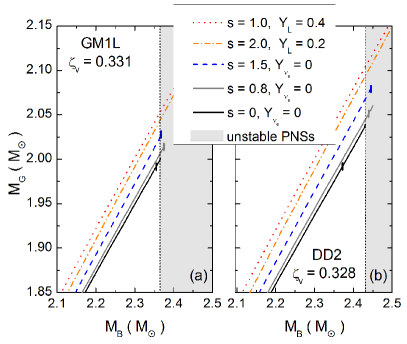
Figure 16: (Color online) Gravitational mass versus baryonic mass of selected stages (characterized by entropy and lepton number) in the evolution of proto-neutron stars to neutron stars, computed for the EOSs of this paper. Each line terminates at the maximum-mass star of each stage. The small vertical bars close to the maximum-masses mark the onset of the hadron-quark phase transition. Only the most massive members of the cold neutron-star sequence are found to have pure quark matter in their cores. Stars in the shaded region are gravitationally unstable.

GM1L and $\mathrm{\zeta_{v}}=0.331$
Stages	$M_{G}~{}[M_{\odot}]$	$R~{}{\rm[km]}$	Core compositions
$s=1.0\,,~{}Y_{L}=0.4$	$2.05$	$12.75$	Pure hadronic
$s=2.0\,,~{}Y_{L}=0.2$	$2.04$	$12.84$	Pure hadronic
$s=1.5\,,~{}Y_{\nu_{e}}=0$	$2.02$	$11.94$	Pure hadronic
$s=0.8\,,~{}Y_{\nu_{e}}=0$	$2.01$	$11.97$	Pure hadronic
$s~{}\,=0.0\,,~{}Y_{\nu_{e}}=0$	$2.00$	$11.90$	Quark-Hybrid

Table 4: Masses, radii, and core compositions of the (proto-) neutron stars with conserved baryonic mass $M_{B}=2.36M_{\odot}$, obtained for the GM1L parametrization.

DD2 and $\mathrm{\zeta_{v}}=0.328$
Stages	$M_{G}~{}[M_{\odot}]$	$R~{}{\rm[km]}$	Core compositions
$s=1.0\,,~{}Y_{L}=0.4$	$2.10$	$13.09$	Pure hadronic
$s=2.0\,,~{}Y_{L}=0.2$	$2.09$	$13.15$	Pure hadronic
$s=1.5\,,~{}Y_{\nu_{e}}=0$	$2.07$	$12.37$	Pure hadronic
$s=0.8\,,~{}Y_{\nu_{e}}=0$	$2.05$	$12.49$	Pure hadronic
$s~{}\,=0.0\,,~{}Y_{\nu_{e}}=0$	$2.04$	$12.27$	Quark-Hybrid

Table 5: Same as Table 4, but for the DD2 parametrization and a conserved baryonic mass of $M_{B}=2.43M_{\odot}$.

It has been proposed Prakash et al. (1997); Brown and Bethe (1994) that the unstable proto-neutron stars mentioned above will collapse to black holes. Moreover, it has been shown in Ref. Prakash et al. (1997); Vidana et al. (2003) that the collapse to a black hole could also be related to the presence of hyperons, $\Delta$-isobars, and/or quarks in the stellar matter, since the hot neutrino-trapped matter is capable of supporting more massive objects than cold stellar matter.

V.4 Tidal deformability of neutron stars

The tidal deformability of neutron stars is an important parameter for gravitational-wave (GW) astronomy as it determines the pre-merger GW signal in NS-NS merger events. To linear order, the tidal deformability, $\lambda$ is given by

$$\lambda=-\frac{\mathcal{E}_{ab}}{Q_{ab}}\,,$$

where $\mathcal{E}_{ab}$ is the applied external field and $Q_{ab}$ the induced mass-quadrupole moment. $\lambda$ is related to the dimensionless tidal Love number, $k_{2}$, associated with $\ell=2$ perturbations,

$$\lambda=\frac{2}{3}k_{2}R^{5}\,,$$

where $R$ denotes the stellar radius. The dimensionless tidal deformability, $\Lambda$, can then be calculated as

$$\Lambda=\lambda/M^{5}\,,$$ (34)

where $M$ denotes the star’s gravitational mass. The tidal Love number can be written in terms of the stellar compactness, $\beta=M/R$, as

$$k_{2}\,=\, \bigg{\{}\frac{8}{5}\beta^{5}(1-2\beta)^{2}\Big{[}2+2\beta(\eta-1)-\eta\Big{]}\bigg{\}}$$

$$\times\bigg{\{}2\beta\Big{[}6-3\eta+3\beta(5\eta-8)\Big{]}$$ (35)

$$+4\beta^{3}\Big{[}13-11\eta+\beta(3\eta-2)+2\beta^{2}(\eta+1)\Big{]}$$

$$+3(1-2\beta)^{2}\Big{[}2-\eta+2\beta(\eta-1)\Big{]}\ln(1-2\beta)\bigg{\}}^{-1}\,,$$

with $\eta=\eta(r=R)$. $\eta(r)$ is the solution of

$$r\frac{{\rm d}\eta}{{\rm d}r} +\eta(r)^{2}+\eta(r){\rm e}^{\lambda(r)}\left[1+4\pi r^{2}\left[P(r)+\epsilon(r)\right]\right]$$ (36)

$$+r^{2}\Xi(r)=0,$$

where

$$\Xi(r) = 4\pi{\rm e}^{\lambda(r)}\left[5\epsilon(r)+9P(r)+\frac{\epsilon(r)+P(r)}{{\rm d}P/{\rm d}\epsilon}\right]$$

$$- 6\frac{{\rm e}^{\lambda(r)}}{r^{2}}-\left(\frac{{\rm d}\nu(r)}{{\rm d}r}\right)^{2}.$$

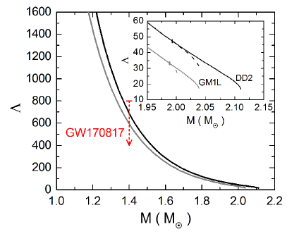
Figure 17: (Color online) Tidal deformability versus gravitational mass of pure hadronic stars (solid lines). Hybrid branches are indicated by dashed lines. The small vertical bars on each curve mark the onset of the phase transition from hadronic to quark matter. Each line terminates at the maximum-mass star. The red arrow shows the constraint on $\Lambda$ imposed by the analysis of the data of GW170817.

Equation (36) it to be solved simultaneously with the TOV equation for the boundary condition $\eta(0)=2$.

When an EoS with a sharp discontinuity at a radius $r=r_{\rm d}$ is used to describe the matter in the interior of a compact object, the additional junction condition

$$\eta(r_{\rm d}^{+})-\eta(r_{\rm d}^{-})=\frac{4\pi r_{\rm d}^{3}\left[\epsilon(r_{\rm d}^{+})-\epsilon(r_{\rm d}^{-})\right]}{m(r_{\rm d})}$$

is to be imposed Han and Steiner (2019).

The data analysis of GW170817 puts constrains on the dimensionless tidal deformability of a $1.4M_{\odot}$ star which is given by $\Lambda_{1.4}\leq 800$ (see, Most et al. (2018b); Raithel et al. (2018b); Abbott et al. (2018); Orsaria et al. (2019) and references therein.)

In Fig. 17 we present the dimensionless tidal deformability as a function of gravitational mass for the cold hybrid stars studied in this work. We also present, for completeness, the results of purely hadronic neutron stars. Due to the high value of the transition pressure, the discrepancies are only noticeable for the high mass objects, being $\sim 10\%$ for the GM1L case and $\sim 20\%$ for the hadronic EoS DD2. The red arrow shows the limit imposed on $\Lambda$ by the analysis of the data from GW170817. As can be seen, our results are in agreement with the observational constraint.

VI Summary and conclusions

This paper had two main objectives. The first objective was to investigate the phase diagram of quark matter using the non-local 3-flavor NJL model coupled to the Polyakov loop. In particular, we studied the possible existence of a spinodal region in the QCD phase diagram and determined the temperature and chemical potential of the critical end point (CEP).

The peaks of the chiral susceptibility of light quarks were used to determine the crossover phase transition (critical points) in the phase diagram. For the first-order transition, the spinodal lines have been determined from the vanishing of the speed-of-sound. As shown in Fukushima (2008a); Contrera et al. (2014), the location of the CEP along the phase transition line depends on the vector-to-scalar interaction strength, $\mathrm{\zeta_{v}}$. We found that considering the vector interactions shrinks the metastable region in the phase diagram, renders quark matter less compressible, and shifts the first-order phase transition to higher chemical potentials.

The second main objective of this paper was to investigate the quark-hadron composition of baryonic matter at zero as well as non-zero temperature. This is of great topical interest for the analysis and interpretation of neutron star merger events such as GW170817. With this in mind, we determined the composition of proto-neutron star matter for entropies and lepton fractions that are typical of such matter. These compositions were used to delineate the evolution of proto-neutron stars to neutron stars in the baryon-mass versus gravitational-mass diagram.

For the treatment of hadronic matter, we used the DDRMF model which takes into account density-dependent meson-baryon coupling constants. Vector meson-hyperon coupling constants were chosen according to the SU(3) ESC08 model, while the scalar meson-hyperon coupling constants were fitted to empirical hypernuclear potentials. This coupling scheme leads to hadronic EoSs (labeled GM1L and DD2) which satisfy the $2\,M_{\odot}$ constraint as well as the constraint on neutron star radii derived from the gravitational-wave event GW170817.

The hadron-quark phase transition was treated as a Maxwell construction, which leads to a sharp hadron-quark interface. The $2\,M_{\odot}$ constraint of PSR J1614-2230 and PSR J0348+0432 and the assumption that quark matter exists in the cores of (cold) neutron stars were used to determine the range of the vector coupling constant $\mathrm{\zeta_{v}}$ in quark matter. This lead to $0.331<\mathrm{\zeta_{v}}<0.371$ for GM1L, and $0.328<\mathrm{\zeta_{v}}<0.385$ for DD2, where the lower bounds follow from the $2\,M_{\odot}$ constraint and the upper bounds from the existence of quark matter in the cores of neutron stars.

The compositions and EoSs of hybrid stars were computed at zero as well as finite temperature, entropies $0\leq s\leq 2$, lepton numbers $0\leq Y_{L}\leq 0.4$, with and without neutrinos. The EoSs were then used to delineate the evolution of proto-neutron stars to neutron stars in the baryon-mass versus gravitational-mass diagram. We found that the hybrid-DD2 EoS with $\mathrm{\zeta_{v}}=0.328$ allows for the existence of hybrid stars up to $T_{\textrm{{trans}}}$= 30 MeV while the hybrid-GM1L EoS with $\mathrm{\zeta_{v}}=0.328$ leads to hybrid configurations with critical temperatures less than $T_{\textrm{{trans}}}$ = 15 MeV. Based on the dense matter models of this work, quark matter existing (by construction) in cold neutron stars, would neither be present in hot neutron stars nor in proto-neutron stars. The situation is drastically different for hyperons and $\Delta$-isobars, which are found to exist very abundantly in proto-neutron star matter.

In closing, we mention that the data provided by gravitational-wave detectors such as LIGO and VIRGO have the potential to shed light on whether or not hybridization and/or quark deconfinement occurs in the cores of neutron stars. Of particular interest in this context is the tidal deformability of neutron stars which depends strongly on the nuclear EoS. As discussed in Abbott et al. (2018); Orsaria et al. (2019) (and references therein), the tidal deformability determined for the colliding neutron stars that lead to the gravitational-wave event GW170817 could provide stringent limits on the existence of quark matter in the interiors of neutron stars. The tidal deformability expresses by how much neutron stars are deformed by tidal forces shortly before they collide. This deformation induces a change in the gravitational potential, which, in turn, leads to characteristic changes in the gravitational-wave signal emitted during the collision. The determination of the tidal deformability, therefore, opens up a new and exciting window into the inner workings of neutron stars. The hope is that the upcoming data collecting runs with Advanced LIGO and Advanced Virgo will provide exciting new insight into the deformability of neutron stars and thus the EoS of super-dense matter itself.

References

- B. Friman and C. Höhne and J. Knoll and S. Leupold and J. Randrup and R. Rapp and P. Senger, (2011) (Eds.) B. Friman and C. Höhne and J. Knoll and S. Leupold and J. Randrup and R. Rapp and P. Senger, (Eds.), Lecture Notes in Physics, Berlin Springer Verlag 814 (2011).
- (2) https://www.gsi.de/en/researchaccelerators/fair.htm.
- Blaschke et al. (2016) D. Blaschke, J. Aichelin, E. Bratkovskaya, V. Friese, M. Gazdzicki, J. Randrup, O. Rogachevsky, O. Teryaev, and V. Toneev, European Physical Journal A 52, 267 (2016).
- (4) http://nica.jinr.ru/.
- (5) https://j-parc.jp/researcher/index-e.html.
- (6) https://home.cern/science/accelerators/super-proton-synchrotron.
- (7) https://www.bnl.gov/bes2015/index.php.
- Roark and Dexheimer (2018) J. Roark and V. Dexheimer, Phys. Rev. C 98, 055805 (2018), URL https://link.aps.org/doi/10.1103/PhysRevC.98.055805.
- Buballa (2005) M. Buballa, Physics Reports 407, 205 (2005), URL http://www.sciencedirect.com/science/article/pii/S037015730400506X.
- Fukushima (2008a) K. Fukushima, Phys. Rev. D77, 114028 (2008a), [Erratum: Phys. Rev.D78,039902(2008)].
- Contrera et al. (2008) G. A. Contrera, D. G. Dumm, and N. N. Scoccola, Phys. Lett. B 661, 113 (2008), URL http://www.sciencedirect.com/science/article/pii/S0370269308001421.
- Contrera, G. A. and Orsaria, M. and Scoccola, N. N. (2010) Contrera, G. A. and Orsaria, M. and Scoccola, N. N., Phys. Rev. D 82, 054026 (2010), URL {http://link.aps.org/doi/10.1103/PhysRevD.82.054026}.
- Carlomagno (2018) J. P. Carlomagno, Phys. Rev. D 97, 094012 (2018), URL https://link.aps.org/doi/10.1103/PhysRevD.97.094012.
- Philipsen (2013) O. Philipsen, Prog. Part. Nucl. Phys. 70, 55 (2013).
- Borsanyi et al. (2014) S. Borsanyi, Z. Fodor, C. Hoelbling, S. D. Katz, S. Krieg, and K. K. Szabo, Phys. Lett. B730, 99 (2014).
- Bellwied et al. (2015) R. Bellwied, S. Borsanyi, Z. Fodor, J. Günther, S. D. Katz, C. Ratti, and K. K. Szabo, Phys. Lett. B751, 559 (2015), eprint 1507.07510.
- Fukushima and Hatsuda (2011) K. Fukushima and T. Hatsuda, Rept. Prog. Phys. 74, 014001 (2011).
- Most et al. (2019) E. R. Most, L. J. Papenfort, V. Dexheimer, M. Hanauske, S. Schramm, H. Stöcker, and L. Rezzolla, Phys. Rev. Lett. 122, 061101 (2019), eprint 1807.03684.
- Bauswein et al. (2019) A. Bauswein, N.-U. F. Bastian, D. B. Blaschke, K. Chatziioannou, J. A. Clark, T. Fischer, and M. Oertel, Phys. Rev. Lett. 122, 061102 (2019), eprint 1809.01116.
- Steinheimer, Jan and Randrup, Jørgen (2012) Steinheimer, Jan and Randrup, Jørgen, Phys. Rev. Lett. 109, 212301 (2012), URL {http://link.aps.org/doi/10.1103/PhysRevLett.109.212301}.
- Steinheimer and Randrup (2016) J. Steinheimer and J. Randrup, The European Physical Journal A 52, 239 (2016), URL http://dx.doi.org/10.1140/epja/i2016-16239-2.
- Sasaki, C. and Friman, B. and Redlich, K. (2007) Sasaki, C. and Friman, B. and Redlich, K., Phys. Rev. Lett. 99, 232301 (2007), URL {http://link.aps.org/doi/10.1103/PhysRevLett.99.232301}.
- Sasaki, C. and Friman, B. and Redlich, K. (2008) Sasaki, C. and Friman, B. and Redlich, K., Phys. Rev. D 77, 034024 (2008), URL {http://link.aps.org/doi/10.1103/PhysRevD.77.034024}.
- Li, Feng and Ko, Che Ming (2017) Li, Feng and Ko, Che Ming, Phys. Rev. C 95, 055203 (2017), URL {https://link.aps.org/doi/10.1103/PhysRevC.95.055203}.
- Schaefer and Shuryak (1998) T. Schaefer and E. V. Shuryak, Rev. Mod. Phys. 70, 323 (1998).
- Roberts and Schmidt (2000) C. D. Roberts and S. M. Schmidt, Prog. Part. Nucl. Phys. 45, S1 (2000).
- Demorest et al. (2010) P. Demorest, T. Pennucci, S. Ransom, M. Roberts, and J. Hessels, Nature 467, 1081 (2010), eprint 1010.5788.
- Lynch et al. (2013) R. S. Lynch et al., Astrophys. J. 763, 81 (2013), eprint 1209.4296.
- Antoniadis et al. (2013) J. Antoniadis et al., Science 340, 6131 (2013), eprint 1304.6875.
- Arzoumanian et al. (2018) Z. Arzoumanian, A. Brazier, S. Burke-Spolaor, S. Chamberlin, S. Chatterjee, B. Christy, J. M. Cordes, N. J. Cornish, F. Crawford, H. T. Cromartie, et al., The Astrophysical Journal Supplement Series 235, 37 (2018), URL https://doi.org/10.3847%2F1538-4365%2Faab5b0.
- Bauswein et al. (2017) A. Bauswein, O. Just, H.-T. Janka, and N. Stergioulas, Astrophys. J. 850, L34 (2017), eprint 1710.06843.
- Fattoyev et al. (2018) F. J. Fattoyev, J. Piekarewicz, and C. J. Horowitz, Phys. Rev. Lett. 120, 172702 (2018), eprint 1711.06615.
- Raithel et al. (2018a) C. Raithel, F. Özel, and D. Psaltis, Astrophys. J. 857, L23 (2018a), eprint 1803.07687.
- Most et al. (2018a) E. R. Most, L. R. Weih, L. Rezzolla, and J. Schaffner-Bielich, Phys. Rev. Lett. 120, 261103 (2018a), eprint 1803.00549.
- Annala et al. (2018) E. Annala, T. Gorda, A. Kurkela, and A. Vuorinen, Phys. Rev. Lett. 120, 172703 (2018), eprint 1711.02644.
- Scarpettini, A. and Gómez Dumm, D. and Scoccola, Norberto N. (2004) Scarpettini, A. and Gómez Dumm, D. and Scoccola, Norberto N., Phys. Rev. D 69, 114018 (2004), URL {http://link.aps.org/doi/10.1103/PhysRevD.69.114018}.
- Carlomagno, J. P. and Gómez Dumm, D. and Scoccola, N. N. (2013) Carlomagno, J. P. and Gómez Dumm, D. and Scoccola, N. N., Phys. Rev. D 88, 074034 (2013), URL {http://link.aps.org/doi/10.1103/PhysRevD.88.074034}.
- Contrera, G. A. and Dumm, D. Gómez and Scoccola, Norberto N. (2010) Contrera, G. A. and Dumm, D. Gómez and Scoccola, Norberto N., Phys. Rev. D 81, 054005 (2010), URL {http://link.aps.org/doi/10.1103/PhysRevD.81.054005}.
- Gomez Dumm and Scoccola (2005) D. Gomez Dumm and N. N. Scoccola, Phys. Rev. C72, 014909 (2005), eprint hep-ph/0410262.
- Rößner, S. and Ratti, C. and Weise, W. (2007) Rößner, S. and Ratti, C. and Weise, W., Phys. Rev. D 75, 034007 (2007), URL {http://link.aps.org/doi/10.1103/PhysRevD.75.034007}.
- Orsaria et al. (2019) M. G. Orsaria, G. Malfatti, M. Mariani, I. F. Ranea-Sandoval, F. García, W. M. Spinella, G. A. Contrera, G. Lugones, and F. Weber, J. Phys. G46, 073002 (2019).
- Tanabashi et al. (2018) M. Tanabashi et al. (Particle Data Group), Phys. Rev. D98, 030001 (2018).
- Contrera et al. (2014) G. A. Contrera, A. G. Grunfeld, and D. B. Blaschke, Phys. Part. Nucl. Lett. 11, 342 (2014).
- Parappilly et al. (2006) M. B. Parappilly, P. O. Bowman, U. M. Heller, D. B. Leinweber, A. G. Williams, and J. B. Zhang, Phys. Rev. D 73, 054504 (2006), URL https://link.aps.org/doi/10.1103/PhysRevD.73.054504.
- Bazavov et al. (2012) A. Bazavov et al., Phys. Rev. D85, 054503 (2012).
- Aoki et al. (2009) Y. Aoki, S. Borsanyi, S. Durr, Z. Fodor, S. D. Katz, S. Krieg, and K. K. Szabo, JHEP 06, 088 (2009).
- Bazavov et al. (2016) A. Bazavov, N. Brambilla, H. T. Ding, P. Petreczky, H. P. Schadler, A. Vairo, and J. H. Weber, Phys. Rev. D93, 114502 (2016).
- Aarts et al. (2017) G. Aarts, C. Allton, D. De Boni, S. Hands, B. Jäger, C. Praki, and J.-I. Skullerud, JHEP 1706, 034 (2017).
- Marczenko et al. (2018) M. Marczenko, D. Blaschke, K. Redlich, and C. Sasaki, Phys. Rev. D 98, 103021 (2018), URL https://link.aps.org/doi/10.1103/PhysRevD.98.103021.
- Klähn et al. (2017) T. Klähn, T. Fischer, and M. Hempel, Astrophys. J. 836, 89 (2017), eprint 1603.03679.
- Zhang and Kunihiro (2009) Z. Zhang and T. Kunihiro, Phys. Rev. D 80, 014015 (2009), URL https://link.aps.org/doi/10.1103/PhysRevD.80.014015.
- Fukushima (2008b) K. Fukushima, Phys. Rev. D78, 114019 (2008b).
- Ratti (2018) C. Ratti, Reports on Progress in Physics 81, 084301 (2018), URL https://doi.org/10.1088%2F1361-6633%2Faabb97.
- Randrup, Jørgen (2009) Randrup, Jørgen, Phys. Rev. C 79, 054911 (2009), URL {http://link.aps.org/doi/10.1103/PhysRevC.79.054911}.
- Randrup, Jørgen (2010) Randrup, Jørgen, Phys. Rev. C 82, 034902 (2010), URL {http://link.aps.org/doi/10.1103/PhysRevC.82.034902}.
- Schmitt (2010) A. Schmitt, Lect. Notes Phys. 811, 1 (2010), eprint 1001.3294.
- Bedaque and Steiner (2015) P. Bedaque and A. W. Steiner, Phys. Rev. Lett. 114, 031103 (2015).
- Typel (2018) S. Typel, Particles 1, 2 (2018).
- Fuchs et al. (1995) C. Fuchs, H. Lenske, and H. H. Wolter, Phys. Rev. C52, 3043 (1995), eprint nucl-th/9507044.
- Rijken et al. (2010) T. A. Rijken, M. M. Nagels, and Y. Yamamoto, Progress of Theoretical Physics Supplement 185, 14 (2010), URL http://dx.doi.org/10.1143/PTPS.185.14.
- Spinella (2017) W. M. Spinella, Ph.D. thesis, Claremont Graduate University & San Diego State University (2017).
- Spinella et al. (2018) W. M. Spinella, F. Weber, M. G. Orsaria, and G. A. Contrera, Universe 4, 64 (2018), eprint 1805.05772.
- Typel et al. (2010) S. Typel, G. Ropke, T. Klähn, D. Blaschke, and H. H. Wolter, Phys. Rev. C81, 015803 (2010), eprint 0908.2344.
- Marczenko and Sasaki (2018) M. Marczenko and C. Sasaki, Phys. Rev. D97, 036011 (2018), eprint 1711.05521.
- Hofmann et al. (2001) F. Hofmann, C. M. Keil, and H. Lenske, Phys. Rev. C 64, 025804 (2001), URL https://link.aps.org/doi/10.1103/PhysRevC.64.025804.
- Prakash et al. (1997) M. Prakash, I. Bombaci, M. Prakash, P. J. Ellis, J. M. Lattimer, and R. Knorren, Physics Reports 280, 1 (1997), ISSN 0370-1573, URL http://www.sciencedirect.com/science/article/pii/S0370157396000233.
- Kajantie et al. (1991) K. Kajantie, L. Kärkkäinen, and K. Rummukainen, Nuclear Physics B 357, 693 (1991), ISSN 0550-3213, URL http://www.sciencedirect.com/science/article/pii/055032139190486H.
- Sotani et al. (2011) H. Sotani, N. Yasutake, T. Maruyama, and T. Tatsumi, Phys. Rev. D 83, 024014 (2011), URL https://link.aps.org/doi/10.1103/PhysRevD.83.024014.
- Yasutake et al. (2014) N. Yasutake, R. Łastowiecki, S. Benić, D. Blaschke, T. Maruyama, and T. Tatsumi, Phys. Rev. C 89, 065803 (2014), URL https://link.aps.org/doi/10.1103/PhysRevC.89.065803.
- Hempel et al. (2013) M. Hempel, V. Dexheimer, S. Schramm, and I. Iosilevskiy, Phys. Rev. C 88, 014906 (2013), URL https://link.aps.org/doi/10.1103/PhysRevC.88.014906.
- Alford et al. (2005) M. Alford, M. Braby, M. Paris, and S. Reddy, The Astrophysical Journal 629, 969 (2005), URL https://doi.org/10.1086%2F430902.
- McLerran and Pisarski (2007) L. McLerran and R. D. Pisarski, Nucl. Phys. A796, 83 (2007), eprint 0706.2191.
- Baym et al. (2018) G. Baym, T. Hatsuda, T. Kojo, P. D. Powell, Y. Song, and T. Takatsuka, Rept. Prog. Phys. 81, 056902 (2018), eprint 1707.04966.
- Blaschke et al. (2009) D. Blaschke, F. Sandin, T. Klähn, and J. Berdermann, Phys. Rev. C 80, 065807 (2009), URL https://link.aps.org/doi/10.1103/PhysRevC.80.065807.
- Krüger et al. (2013) T. Krüger, I. Tews, K. Hebeler, and A. Schwenk, Phys. Rev. C88, 025802 (2013), eprint 1304.2212.
- Hebeler et al. (2013) K. Hebeler, J. M. Lattimer, C. J. Pethick, and A. Schwenk, Astrophys. J. 773, 11 (2013), eprint 1303.4662.
- Kurkela et al. (2014) A. Kurkela, E. S. Fraga, J. Schaffner-Bielich, and A. Vuorinen, Astrophys. J. 789, 127 (2014), eprint 1402.6618.
- Tolman (1939) R. C. Tolman, Phys. Rev. 55, 364 (1939).
- Ruester et al. (2005) S. B. Ruester, V. Werth, M. Buballa, I. A. Shovkovy, and D. H. Rischke, Phys. Rev. D72, 034004 (2005), eprint hep-ph/0503184.
- Alvarez-Castillo et al. (2019) D. E. Alvarez-Castillo, D. B. Blaschke, A. G. Grunfeld, and V. P. Pagura, Phys. Rev. D99, 063010 (2019), eprint 1805.04105.
- Blaschke et al. (2005) D. Blaschke, S. Fredriksson, H. Grigorian, A. M. Öztaş, and F. Sandin, Phys. Rev. D 72, 065020 (2005), URL https://link.aps.org/doi/10.1103/PhysRevD.72.065020.
- Pons et al. (1999) J. A. Pons, S. Reddy, M. Prakash, J. M. Lattimer, and J. A. Miralles, The Astrophysical Journal 513, 780 (1999), URL https://doi.org/10.1086%2F306889.
- Brown and Bethe (1994) G. E. Brown and H. Bethe, Astrophys. J. 423, 659 (1994).
- Vidana et al. (2003) I. Vidana, I. Bombaci, A. Polls, and A. Ramos, Astron. Astrophys. 399, 687 (2003), eprint astro-ph/0209068.
- Han and Steiner (2019) S. Han and A. W. Steiner, Phys. Rev. D 99, 083014 (2019), URL https://link.aps.org/doi/10.1103/PhysRevD.99.083014.
- Most et al. (2018b) E. R. Most, L. R. Weih, L. Rezzolla, and J. Schaffner-Bielich, Phys. Rev. Lett. 120, 261103 (2018b), eprint 1803.00549.
- Raithel et al. (2018b) C. Raithel, F. Özel, and D. Psaltis, Astrophys. J. 857, L23 (2018b), eprint 1803.07687.
- Abbott et al. (2018) B. P. Abbott et al. (LIGO Scientific, Virgo), Phys. Rev. Lett. 121, 161101 (2018), eprint 1805.11581.