keys-valuespython/artifacts/keys-values.csv
Sparsely Activated Networks
Abstract
Previous literature on unsupervised learning focused on designing structural priors with the aim of learning meaningful features. However, this was done without considering the description length of the learned representations which is a direct and unbiased measure of the model complexity. In this paper, first we introduce the metric that evaluates unsupervised models based on their reconstruction accuracy and the degree of compression of their internal representations. We then present and define two activation functions (Identity, ReLU) as base of reference and three sparse activation functions (top-k absolutes, Extrema-Pool indices, Extrema) as candidate structures that minimize the previously defined . We lastly present Sparsely Activated Networks (SANs) that consist of kernels with shared weights that, during encoding, are convolved with the input and then passed through a sparse activation function. During decoding, the same weights are convolved with the sparse activation map and subsequently the partial reconstructions from each weight are summed to reconstruct the input. We compare SANs using the five previously defined activation functions on a variety of datasets (Physionet, UCI-epilepsy, MNIST, FMNIST) and show that models that are selected using have small description representation length and consist of interpretable kernels.
Index Terms:
artificial neural networks, autoencoders, compression, sparsityI Introduction
Deep Neural Networks (DNNs) [1] use multiple stacked layers containing weights and activation functions, that transform the input to intermediate representations during the feed-forward pass. Using backpropagation [2] the gradient of each weight w.r.t. the error of the output is efficiently calculated and passed to an optimization function such as Stochastic Gradient Descent or Adam [3] which updates the weights making the output of the network converge to the desired output. DNNs were successful in utilizing big data and powerful parallel processing units and achieved state-of-the-art performance in problems such as image [4] and speech recognition [5]. However, these breakthroughs have come at the expense of increased description length of the learned representations, which in sparsely represented DNNs is proportional with the number of:
-
•
weights of the model and
-
•
non-zero activations.
The use of large number of weights as a design choice in architectures such as Inception [6], VGGnet [7] and ResNet [8] (usually by increasing the depth) was followed by research that signified the weight redundancy of DNNs. It was demonstrated that DNNs easily fit random labeling of the data [9] and that in any DNN there exists a subnetwork that can solve the given problem with the same accuracy with the original one [10].
Moreover, DNNs with large number of weights have higher storage requirements and they are slower during inference. Previous literature addressing this problem has focused on weight pruning from trained DNNs [11] and weight pruning during training [12]. Pruning minimizes the model capacity for use in environments with low computational capabilities, or low inference time requirements and helps reducing co-adaptation between neurons, a problem which was also addressed by the use Dropout [13]. Pruning strategies however, only take in consideration the number of weights of the model.
The other element that affects the description length of the representation of DNNs is the number of non-zero activations in the intermediate representations which is related with the concept of activity sparseness. In neural networks sparseness can be applied on the connections between neurons, or in the activation maps [14]. Although sparseness in the activation maps is usually enforced in the loss function by adding a regularization or Kullback-Leibler divergence term [15], we could also achieve sparsity in the activation maps with the use of an appropriate activation function.
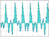
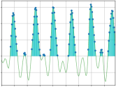
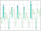
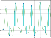
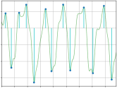
Initially, bounded functions such as and were used, however besides producing dense activation maps they also present the vanishing gradients problem [16]. Rectified Linear Units (ReLUs) were later proposed [17, 18] as an activation function that solves the vanishing gradients problem and increases the sparsity of the activation maps. Although ReLU creates exact zeros (unlike its predecessors and ), its activation map consists of sparsely separated but still dense areas (Fig. 1LABEL:sub@subfig:relu) instead of sparse spikes. The same applies for generalizations of ReLU, such as Parametric ReLU [19] and Maxout [20]. Recently, in -Sparse Autoencoders [21] the authors used an activation function that applies thresholding until the most active activations remain, however this non-linearity covers a limited area of the activation map by creating sparsely disconnected dense areas (Fig. 1LABEL:sub@subfig:topkabsolutes), similar to the ReLU case.
Moreover activation functions that produce continuous valued activation maps (such as ReLU) are less biologically plausible, because biological neurons rarely are in their maximum saturation regime [22] and use spikes to communicate instead of continuous values [23]. Previous literature has also demonstrated the increased biological plausibility of sparseness in artificial neural networks [24]. Spike-like sparsity on activation maps has been thoroughly researched on the more biologically plausible rate-based network models [25], but it has not been thoroughly explored as a design option for activation functions combined with convolutional filters.
The increased number of weights and non-zero activations make DNNs more complex, and thus more difficult to use in problems that require corresponding causality of the output with a specific set of neurons. The majority of domains where machine learning is applied, including critical areas such as healthcare [26], require models to be interpretable and explainable before considering them as a solution. Although these properties can be increased using sensitivity analysis [27], deconvolution methods [28], Layerwise-Relevance Propagation [29] and Local-Interpretable Model agnostic Explanations [30] it would be preferable to have self-interpretable models.
Moreover, considering that DNNs learn to represent data using the combined set of trainable weights and non-zero activations during the feed-forward pass, an interesting question arises:
What are the implications of trading off the reconstruction error of the representations with their compression ratio w.r.t to the original data?
Previous work by Blier et al. [31] demonstrated the ability of DNNs to losslessly compress the input data and the weights, but without considering the number of non-zero activations. In this work we relax the lossless requirement and also consider neural networks purely as function approximators instead of probabilist models. The contributions of this paper are the following proposals:
-
•
The metric that evaluates unsupervised models based on how compressed their learned representations are w.r.t the original data and how accurate their reconstruction is.
- •
In Section II we define the metric, then in Section III we define the five tested activation functions along with the architecture and training procedure of SANs, in Section IV we experiment SANs on the Physionet [32], UCI-epilepsy [33], MNIST [34] and FMNIST [35] databases and provide visualizations of the intermediate representations and results. In Section V we discuss the findings of the experiments and the limitations of SANs and finally in Section VI we present the concluding remarks and the future work.
II Metric
Let be a model with kernels each one with samples and a reconstruction loss function for which we have:
| (1) |
, where is the input vector and is a reconstruction of . For the definition of metric we use a neural network model that consists of convolutional filters, however this can be easily generalized to other architectures.
The metric evaluates a model based on two concepts: its verbosity and its accuracy. Verbosity in neural networks can be perceived as inversely proportional to the compression ratio of the representations. We calculate the number of weights of as follows:
| (2) |
We also calculate the number of non-zero activations of for input as:
| (3) |
, where denotes the pseudo-norm and is the activation map of the kernel. Then using Equations 2 and 3 we define the compression ratio of w.r.t as:
| (4) |
, where denotes dimensionality and was previously defined as the cardinality of . The reason that we multiply the dimensionality of with the number of activations is that we need to consider the spatial position of each non-zero activation in addition to its amplitude to reconstruct . Moreover, using that definition of , there is a desirable trade-off between using a larger kernel with less instances and a smaller kernel with more instances based on which kernel size minimizes the . This definition of allows us to set a base of reference for for models that their representational capacity is equal with the number of samples of the input.
Regarding the accuracy, we define the normalized reconstruction loss as follows:
| (5) |
This definition of allows us to set a base of reference for in cases when the reconstruction the model performs is equivalent with a model that performs constant reconstructions independent of the input. Finally using Equations 4 and 5 we define the 111The use of the symbol comes from the first character of the combined greek word \textgreekfontφλύθος = \textgreekfontφλύ+θος (flithos: pronounced as flee-thos). It consists of the first part of the word \textgreekfontφλύ-αρος (meaning verbose) and the second part of \textgreekfontλά-θος (meaning wrong). \textgreekfontΦλύθος is literally defined as: Giving inaccurate information using many words; the state of being wrong and wordy at the same time. metric of w.r.t as follows:
| (6) |
, where denotes the euclidean-norm. The rationale behind defining is to satisfy the need for a unified metric that takes in consideration both the ‘verbosity’ of a model along with its ‘accuracy’.
Regarding hyperparameter selection we also define the mean of a dataset or a mini-batch w.r.t to as:
| (7) |
, where is the number of observations in the dataset or the batch size.
is non-differentiable due to the presence of the pseudo-norm in Eq. 3. A way to overcome this is using as the differentiable optimization function during training and as the metric for model selection during validation on which hyperparameter value decisions (such as kernel size) are made.
III Sparsely Activated Networks
III-A Sparse Activation Functions
In this subsection we define five activation functions and their corresponding sparsity density parameter for which we have:
| (8) |
We choose values for for each activation function in such as way, to approximately have the same number of activations for fair comparison of the sparse activation functions.
III-A1 Identity
. The Identity activation function serves as a baseline and does not change its input as shown in Fig. 1LABEL:sub@subfig:identity. For this case does not apply.
III-A2 ReLU
. The ReLU activation function produces sparsely disconnected but internally dense areas as shown in Fig. 1LABEL:sub@subfig:relu instead of sparse spikes. For this case does not apply.
III-A3 top-k absolutes
The top-k absolutes function (defined at Algorithm 1) keeps the indices of activations with the largest absolute value and zeros out the rest, where . We set , where . Top-k absolutes is sparser than ReLU but some extrema are overactivated related to some others that are not activated at all, as shown in Fig. 1LABEL:sub@subfig:topkabsolutes.
III-A4 Extrema-Pool indices
The Extrema-Pool indices activation function (defined at Algorithm 2) keeps only the index of the activation with the maximum absolute amplitude from each region outlined by a grid as granular as the kernel size and zeros out the rest. It consists of a max-pooling layer followed by a max-unpooling layer with the same parameters while the sparsity parameter in this case is set . This activation function creates sparser activation maps than top-k absolutes however in cases where the pool grid is near a peak or valley this region is activated twice (as shown in Fig. 1LABEL:sub@subfig:extremapoolindices).
III-A5 Extrema
The Extrema activation function (defined at Algorithm 3) detects candidate extrema using zero crossing of the first derivative, then sorts them in an descending order and gradually eliminates those extrema that have less absolute amplitude than a neighboring extrema within a predefined minimum extrema distance (). Imposing a on the extrema detection algorithm makes sparser than the previous cases and solves the problem of double extrema activations that Extrema-Pool indices have (as shown in Fig. 1LABEL:sub@subfig:extrema). The sparsity parameter in this case is set , where is the minimum extrema distance. We set for utilizing fair comparison between the sparse activation functions. Specifically for Extrema activation function we introduce a ‘border tolerance’ parameter to allow neuron activation within another neuron activated area.
III-B SAN Architecture/Training
Let be a single input data, however the following can be trivially generalized for batch inputs with different cardinalities. Let the weight matrix of the kernel, that are initialized using a normal distribution with mean and standard deviation :
| (9) |
, where is the number of kernels.
First we calculate the similarity matrices222Previous literature refers it as the ‘hidden variable’ but we use a more direct naming that suits the context of this paper. for each of the weight matrices :
| (10) |
, where is the convolution333We use convolution instead of cross-correlation only as a matter of compatibility with previous literature and computational frameworks. Using cross-correlation would produce the same results and would not require flipping the kernels during visualization. operation. Sufficient padding with zeros is applied on the boundaries to retain the original input size. We do not need a bias term because it would be applied globally on which is almost equivalent with learning the baseline of .
We then pass and a sparsity parameter in the sparse activation function resulting in the activation map :
| (11) |
, where is a sparse matrix that its non-zero elements denote the spatial positions of the instances of the kernel. The exact form of and depends on the choice of the sparse activation function which are presented in Section III-A.
We convolve each with its corresponding resulting in the set of which are partial reconstructions of the input:
| (12) |
, consisting of sparsely reoccurring patterns of with varying amplitude. Finally we can reconstruct the input as the sum of the partial reconstructions as follows:
| (13) |
The Mean Absolute Error (MAE) of the input and the prediction is then calculated:
| (14) |
, where the index denotes the sample. The choice of MAE is based on the need to handle outliers in the data with the same weight as normal values. However, SANs are not restricted in using MAE and other loss functions could be used, such as Mean Square Error.
Using backpropagation, the gradients of the loss w.r.t the are calculated:
| (15) |
Lastly the are updated using the following learning rule:
| (16) |
, where is the learning rate.
After training, we consider (which is calculated during the feed-forward pass from Eq. 11) and (which is calculated using backpropagation from Eq. 16) the compressed representation of , which can be reconstructed using Equations 12 and 13:
| (17) |
Regarding the metric and considering Eq. 17 our target is to estimate an as accurate as possible representation of through and with the least amount of number of non-zero activations and weights.
The general training procedure of SANs for multiple epochs using batches (instead of one example as previously shown) is presented in Algorithm 4.
IV Experiments
For all experiments the weights of the SAN kernels are initialized using the normal distribution with and . We used Adam [3] as the optimizer with learning rate , , , epsilon without weight decay. For implementing and training SANs we used Pytorch [36] with a NVIDIA Titan X Pascal GPU 12GB RAM and a 12 Core Intel i7–8700 CPU @ 3.20GHz on a Linux operating system.
IV-A Comparison of for sparse activation functions and various kernel sizes in Physionet
We study the effect on , of the combined choice of the kernel size and the sparse activation functions that were defined in Section III-A.
IV-A1 Datasets
We use one signal from each of 15 signal datasets from Physionet listed in the first column of Table I. Each signal consists of samples which in turn is split in signals of samples each, to create the training ( signals), validation ( signals) and test datasets ( signals). The only preprocessing that is done is mean subtraction and division of one standard deviation on the samples signals.
IV-A2 Experiment Setup
We train five SANs (one for each sparse activation function) for each of the Physionet datasets, for epochs with a batch size of with one kernel of varying size in the range . During validation we selected the models with the kernel size that achieved the best out of all epochs. During testing we feed the test data into the selected model and calculate , and for this set of hyperparameters as shown in Table I. For Extrema activation we set a ‘border tolerance’ of three samples.
IV-A3 Results
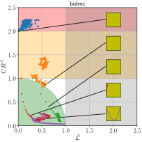
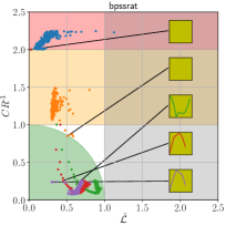
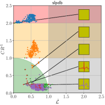
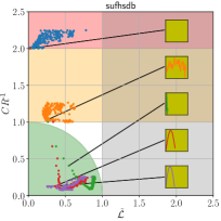
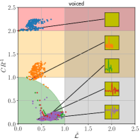
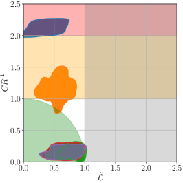
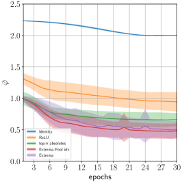
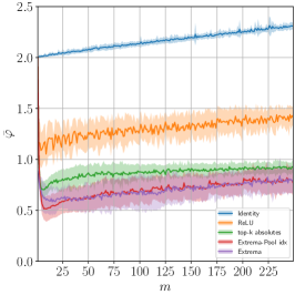
The three separate clusters which are depicted in Fig. 3 and the aggregated density plot in Fig. 4LABEL:sub@subfig:crrl_density_plot between the Identity activation function, the ReLU and the rest show the effect of a sparser activation function on the representation. The sparser an activation function is the more it compresses, sometimes at the expense of reconstruction error. However, by visual inspection of Fig. 5 one could confirm that the learned kernels of the SAN with sparser activation maps (Extrema-Pool indices and Extrema) correspond to the reoccurring patterns in the datasets, thus having high interpretability. These results suggest that reconstruction error by itself is not a sufficient metric for decomposing data in interpretable components. Trying to solely achieve lower reconstruction error (such as the case for the Identity activation function) produces noisy learned kernels, while using the combined measure of reconstruction error and compression ratio (smaller ) results in interpretable kernels. Comparing the differences of between the Identity, the ReLU and the rest sparse activation functions in Fig. 4LABEL:sub@subfig:flithos_m we notice that the latter produce a minimum region in which we observe interpretable kernels.

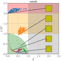
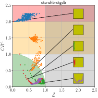
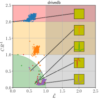
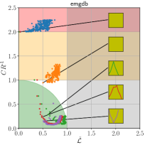
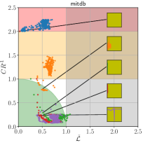
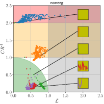
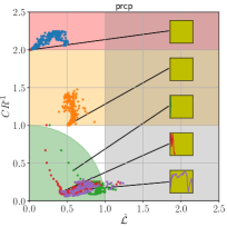
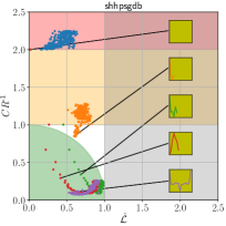


Identity ReLU top-k absolutes Extrema-Pool idx Extrema Datasets apnea-ecg 1 2.00 0.03 2.00 19 0.70 0.53 0.87 74 0.10 0.37 0.39 51 0.09 0.47 0.48 72 0.10 0.31 0.32 bidmc 1 2.00 0.04 2.00 4 0.82 0.50 0.96 5 0.41 0.64 0.76 10 0.21 0.24 0.32 113 0.13 0.30 0.32 bpssrat 1 2.00 0.02 2.00 1 0.85 0.51 0.99 10 0.21 0.63 0.67 8 0.26 0.45 0.52 8 0.24 0.30 0.38 cebsdb 1 2.00 0.01 2.00 3 0.95 0.51 1.07 5 0.41 0.62 0.74 12 0.18 0.21 0.28 71 0.09 0.45 0.46 ctu-uhb-ctgdb 1 2.00 0.01 2.00 1 0.48 0.51 0.71 7 0.29 0.60 0.66 9 0.23 0.44 0.49 45 0.07 0.57 0.57 drivedb 1 2.00 0.04 2.00 20 0.51 0.54 0.74 20 0.12 0.67 0.68 13 0.17 0.69 0.71 19 0.10 0.72 0.73 emgdb 1 2.00 0.04 2.00 1 0.94 0.50 1.07 7 0.29 0.62 0.68 9 0.23 0.48 0.53 7 0.15 0.51 0.53 mitdb 1 2.00 0.03 2.00 61 0.78 0.49 0.92 7 0.29 0.52 0.59 10 0.21 0.44 0.49 229 0.24 0.38 0.45 noneeg 1 2.00 0.01 2.00 6 0.91 0.57 1.08 4 0.50 0.59 0.77 37 0.09 0.49 0.50 15 0.12 0.36 0.38 prcp 1 2.00 0.03 2.00 1 1.00 0.51 1.12 5 0.41 0.59 0.71 23 0.11 0.41 0.42 105 0.12 0.42 0.44 shhpsgdb 1 2.00 0.02 2.00 4 0.85 0.60 1.05 6 0.34 0.69 0.77 7 0.29 0.42 0.51 15 0.10 0.53 0.54 slpdb 1 2.00 0.03 2.00 7 0.72 0.53 0.90 7 0.29 0.52 0.60 232 0.24 0.29 0.37 218 0.23 0.36 0.43 sufhsdb 1 2.00 0.03 2.00 38 1.02 0.24 1.05 5 0.41 0.55 0.68 18 0.13 0.36 0.39 17 0.12 0.26 0.28 voiced 1 2.00 0.01 2.00 41 0.95 0.26 0.98 36 0.09 0.56 0.57 70 0.10 0.41 0.43 67 0.10 0.41 0.43 wrist 1 2.00 0.04 2.00 56 0.74 0.62 0.96 5 0.41 0.49 0.63 9 0.23 0.43 0.49 173 0.18 0.46 0.50
IV-B Evaluation of the reconstruction of SANs using a Supervised CNN on UCI-epilepsy
We study the quality of the reconstructions of SANs by training a supervised 1D Convolutional Neural Network (CNN) on the output of each SAN. We also study the effect that has on and the accuracy of the classifier for the five sparse activation functions.
IV-B1 Dataset
We use the UCI-epilepsy recognition dataset that consists of signals each one with samples (23.5 seconds). The dataset is annotated into five classes with signals for each class. For the purposes of this paper we use a variation of the database444https://archive.ics.uci.edu/ml/datasets/Epileptic+Seizure+Recognition in which the EEG signals are split into segments with samples each, resulting in a balanced dataset that consists of EEG signals in total.
IV-B2 Experiment Setup
First, we merge the tumor classes ( and ) and the eyes classes ( and ) resulting in a modified dataset of three classes (tumor, eyes, epilepsy). We then split the signals into , and ( signals) as training, validation and test data respectively and normalize in the range using the global max and min. For the SANs, we used two kernels with a varying size in the range of and trained for epochs with a batch size of . After training, we choose the model that performed the lowest out of all epochs.
During supervised learning the weights of the kernels are frozen and a CNN is stacked on top of the reconstruction output of the SANs. The CNN feature extractor consists of two convolutional layers with and filters and kernel size , each one followed by a ReLU and a Max-Pool with pool size . The classifier consists of three fully connected layers with , and units. The first two fully connected layers are followed by a ReLU while the last one produces the predictions. The CNN is trained for an additional epochs with the same batch size and model selection procedure as with SANs and categorical cross-entropy as the loss function. For Extrema activation we set a ‘border tolerance’ of two samples.
IV-B3 Results
As shown in Table. II, although we use a significantly reduced representation size, the classification accuracy differences (A%) are retained which suggests that SANs choose the most important features to represent the data. For example for for the Extrema activation function, there is an increase in accuracy of (the baseline CNN on the original data achieved ) although a reduced representation is used with only of the size w.r.t the original data.
Identity ReLU top-k absolutes Extrema-Pool idx Extrema A% A% A% A% A% 8 4.09 0.04 4.09 +5.6 2.09 0.02 2.09 +4.3 0.58 0.73 0.93 -0.4 0.58 0.41 0.71 -7.8 0.37 0.45 0.59 +2.8 9 4.10 0.03 4.10 +1.4 2.10 0.03 2.10 -44.3 0.53 0.74 0.91 -1.2 0.53 0.41 0.67 -2.6 0.35 0.42 0.56 +0.8 10 4.11 0.02 4.11 +8.0 3.61 0.11 3.62 -26.6 0.49 0.76 0.91 -13.4 0.49 0.43 0.65 +1.7 0.35 0.42 0.56 +2.4 11 4.12 0.02 4.12 -44.3 2.12 0.03 2.13 +6.2 0.48 0.76 0.90 -12.2 0.48 0.41 0.63 -1.2 0.34 0.41 0.54 +1.0 12 4.13 0.02 4.13 +6.6 2.13 0.03 2.13 +2.1 0.45 0.77 0.89 -5.7 0.45 0.44 0.63 -1.9 0.34 0.42 0.55 +3.0 13 4.15 0.06 4.15 +4.1 2.15 0.03 2.15 +6.5 0.44 0.78 0.89 -13.5 0.44 0.44 0.62 -9.3 0.34 0.42 0.55 +0.8 14 4.16 0.06 4.16 +6.2 3.66 0.11 3.66 -44.3 0.43 0.78 0.89 -10.4 0.43 0.46 0.63 -2.1 0.34 0.43 0.55 -1.4 15 4.17 0.03 4.17 +9.1 2.17 0.03 2.17 -8.4 0.42 0.78 0.89 -3.5 0.42 0.46 0.62 +1.8 0.34 0.43 0.55 -2.0
IV-C Evaluation of the reconstruction of SANs using a Supervised FNN on MNIST and FMNIST
IV-C1 Dataset
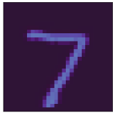
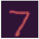
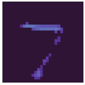
For the same task as the previous one but for 2D, we use MNIST which consists of a training dataset of greyscale images with handwritten digits and a test dataset of images each one having size of . The exact same procedure is used for FMNIST [35].
IV-C2 Experiment Setup
The models consist of two kernels with a varying size in the range of . We use images from the training dataset as a validation dataset and train on the rest for epochs with a batch size of . We do not apply any preprocessing on the images.
During supervised learning the weights of the kernels are frozen and a one layer fully connected network (FNN) is stacked on top of the reconstruction output of the SANs. The FNN is trained for an additional epochs with the same batch size and model selection procedure as with SANs and categorical cross-entropy as the loss function. For Extrema activation we set a ‘border tolerance’ of two samples.
IV-C3 Results
As shown in Table. III the accuracies achieved by the reconstructions of some SANs do not drop proportionally compared to those of an FNN trained on the original data (), although they have been heavily compressed. It is interesting to note that in some cases SANs reconstructions, such as for the Extrema-Pool indices, performed even better than the original data. This suggests the overwhelming presence of redundant information that resides in the raw pixels of the original data and further indicates that SANs extract the most representative features of the data.
Identity ReLU top-k absolutes Extrema-Pool idx Extrema A% A% A% A% A% 1 1.16 0.00 1.16 -0.1 1.16 0.01 1.16 -1.6 1.16 0.00 1.16 -0.3 1.16 0.00 1.16 -0.1 0.09 0.89 0.90 -11.3 2 1.55 0.01 1.55 -0.3 0.78 0.01 0.78 -0.0 1.37 0.02 1.37 -0.6 0.48 0.61 0.79 +1.3 0.09 0.83 0.83 -7.6 3 1.93 0.00 1.93 -0.5 1.16 0.03 1.16 -0.8 0.63 0.25 0.68 -1.6 0.30 0.51 0.59 +0.0 0.08 0.50 0.51 -7.3 4 2.30 0.03 2.30 -0.5 1.53 0.02 1.53 -0.6 0.39 0.40 0.55 -3.7 0.22 0.59 0.63 -0.6 0.07 0.56 0.57 -10.3 5 2.66 0.09 2.66 -0.8 0.73 0.03 0.73 -0.2 0.20 0.55 0.59 -5.3 0.16 0.60 0.62 -0.7 0.07 0.57 0.57 -8.8 6 3.02 0.06 3.02 -0.6 0.60 0.01 0.60 -0.5 0.14 0.61 0.63 -8.8 0.12 0.63 0.65 -1.7 0.05 0.60 0.61 -11.4
Identity ReLU top-k absolutes Extrema-Pool idx Extrema A% A% A% A% A% 1 3.00 0.01 3.00 -1.7 1.50 0.00 1.50 +1.0 3.00 0.01 3.00 -0.5 3.00 0.01 3.00 -3.8 0.35 0.86 0.93 -4.0 2 3.58 0.01 3.58 +2.0 3.00 0.05 3.00 +1.3 1.50 0.31 1.55 -5.0 0.99 0.58 1.16 -0.6 0.23 0.81 0.84 -6.6 3 3.94 0.05 3.94 +2.0 2.01 0.02 2.01 +1.0 0.63 0.63 0.89 -7.0 0.48 0.52 0.72 -0.7 0.16 0.65 0.68 -9.3 4 4.22 0.06 4.22 -0.1 0.01 1.00 1.00 -71.5 0.39 0.69 0.79 -9.4 0.32 0.61 0.70 -1.9 0.09 0.70 0.71 -9.6 5 4.45 0.04 4.45 +1.8 1.92 0.02 1.92 +1.3 0.20 0.75 0.78 -15.0 0.19 0.60 0.63 -5.0 0.07 0.64 0.64 -12.2 6 4.70 0.04 4.70 +0.8 2.80 0.05 2.80 +2.2 0.14 0.77 0.78 -19.6 0.13 0.66 0.67 -4.3 0.05 0.69 0.70 -13.7
V Discussion
SANs combined with the metric compress the description of the data in a way a minimum description language framework would, by encoding them into and . The experiments done in Section IV show that the use of Identity, ReLU and (in a lesser degree) top-k absolutes produce noisy features, while on the other hand Extrema-Pool indices and Extrema produce more robust features and can be configured with parameters (kernel size and ) with values that can be derived by simple visual inspection of the data.
From the point of view of Sparse Dictionary Learning, SANs kernels could be seen as the atoms of a learned dictionary specializing in interpretable pattern matching (e.g. for Electrocardiogram (ECG) input the kernels of SANs are ECG beats) and the sparse activation map as the representation. The fact that SANs are wide with fewer larger kernel sizes instead of deep with smaller kernel sizes make them more interpretable than the DNNs and in some cases without sacrificing significant accuracy.
An advantage of SANs compared to Sparse Autoencoders [37] is that the constrain of activation proximity can be applied individually in each example instead of requiring the computation of forward-pass of all examples. Additionally, SANs create exact zeros instead near-zeros, which reduces co-adaptation between instances of the neuron activation.
could be seen as an alternative formalization of Occam’s razor [38] to Solomonov’s theory of inductive inference [39] but with a deterministic interpretation instead of a probabilistic one. The cost of the description of the data could be seen as proportional to the number of weights and the number of non-zero activations, while the quality of the description is proportional to the reconstruction loss. The metric is also related to the rate-distortion theory [40], in which the maximum distortion is defined according to human perception, which however inevitably introduces a bias. There is also relation with the field of Compressed Sensing [41] in which the sparsity of the data is exploited allowing us to reconstruct it with fewer samples than the Nyquist-Shannon theorem requires and the field of Robust Feature Extraction [42] where robust features are generated with the aim to characterize the data. Olshausen et al. [43] presented an objective function that considers subjective measures of sparseness of the activation maps, however in this work we use the direct measure of compression ratio. Previous work by [44] have used a weighted combination of the number of neurons, percentage root-mean-squared difference and a correlation coefficient for the optimization function of a FNN as a metric but without taking consideration the number of non-zero activations.
A limitation of SANs is the use of varying amplitude-only kernels, which are not sufficient for more complex data and also do not fully utilize the compressibility of the data. A possible solution would be using a grid sampler [45] on the kernel allowing it to learn more general transformations (such as scale) than simple amplitude variability. However, additional kernel properties should be chosen in correspondence with the metric i.e. the model should compress more with decreased reconstruction loss.
VI Conclusions and future work
In this paper first we defined the metric to evaluate how well do models trade-off reconstruction loss with compression. We then defined SANs which have minimal structure and with the use of sparse activation functions learn to compress data without losing important information. Using Physionet datasets and MNIST we demonstrated that SANs are able to create high quality representations with interpretable kernels.
The minimal structure of SANs makes them easy to use for feature extraction, clustering and time-series forecasting. Other future work on SANs include:
-
•
Applying cosine annealing to the extrema distance in order to increase the degree of freedom of the kernels.
-
•
Imposing the minimum extrema distance along all similarity matrices for multiple kernels, thus making kernels compete for territory.
-
•
Applying dropout at the activations in order to correct weights that have overshot, especially when they are initialized with high values. However, the effect of dropout on SANs would generally be negative since SANs have much less weights than DNNs thus need less regularization.
-
•
Using SANs with dynamically created kernels that might be able to learn multimodal data from variable sources (e.g. from ECG to respiratory) without destroying previous learned weights.
ACKNOWLEDGMENT
This work was supported by the European Union’s Horizon 2020 research and innovation programme under Grant agreement 769574. We gratefully acknowledge the support of NVIDIA with the donation of the Titan X Pascal GPU used for this research.
References
- [1] Y. LeCun, Y. Bengio, and G. Hinton, “Deep learning,” nature, vol. 521, no. 7553, p. 436, 2015.
- [2] D. E. Rumelhart, G. E. Hinton, and R. J. Williams, “Learning representations by back-propagating errors,” nature, vol. 323, no. 6088, p. 533, 1986.
- [3] D. P. Kingma and J. Ba, “Adam: A method for stochastic optimization,” arXiv preprint arXiv:1412.6980, 2014.
- [4] A. Krizhevsky, I. Sutskever, and G. E. Hinton, “Imagenet classification with deep convolutional neural networks,” in Advances in neural information processing systems, 2012, pp. 1097–1105.
- [5] A. Graves, A.-r. Mohamed, and G. Hinton, “Speech recognition with deep recurrent neural networks,” in 2013 IEEE international conference on acoustics, speech and signal processing. IEEE, 2013, pp. 6645–6649.
- [6] C. Szegedy, V. Vanhoucke, S. Ioffe, J. Shlens, and Z. Wojna, “Rethinking the inception architecture for computer vision,” in Proceedings of the IEEE conference on computer vision and pattern recognition, 2016, pp. 2818–2826.
- [7] K. Simonyan and A. Zisserman, “Very deep convolutional networks for large-scale image recognition,” arXiv preprint arXiv:1409.1556, 2014.
- [8] K. He, X. Zhang, S. Ren, and J. Sun, “Deep residual learning for image recognition,” in Proceedings of the IEEE conference on computer vision and pattern recognition, 2016, pp. 770–778.
- [9] C. Zhang, S. Bengio, M. Hardt, B. Recht, and O. Vinyals, “Understanding deep learning requires rethinking generalization,” arXiv preprint arXiv:1611.03530, 2016.
- [10] J. Frankle and M. Carbin, “The lottery ticket hypothesis: Finding sparse, trainable neural networks,” in International Conference on Learning Representations, 2019.
- [11] A. Aghasi, A. Abdi, N. Nguyen, and J. Romberg, “Net-trim: Convex pruning of deep neural networks with performance guarantee,” in Advances in Neural Information Processing Systems, 2017, pp. 3177–3186.
- [12] J. Lin, Y. Rao, J. Lu, and J. Zhou, “Runtime neural pruning,” in Advances in Neural Information Processing Systems, 2017, pp. 2181–2191.
- [13] N. Srivastava, G. Hinton, A. Krizhevsky, I. Sutskever, and R. Salakhutdinov, “Dropout: a simple way to prevent neural networks from overfitting,” The journal of machine learning research, vol. 15, no. 1, pp. 1929–1958, 2014.
- [14] S. B. Laughlin and T. J. Sejnowski, “Communication in neuronal networks,” Science, vol. 301, no. 5641, pp. 1870–1874, 2003.
- [15] D. P. Kingma and M. Welling, “Auto-encoding variational bayes,” arXiv preprint arXiv:1312.6114, 2013.
- [16] Y. Bengio, P. Simard, P. Frasconi et al., “Learning long-term dependencies with gradient descent is difficult,” IEEE transactions on neural networks, vol. 5, no. 2, pp. 157–166, 1994.
- [17] X. Glorot, A. Bordes, and Y. Bengio, “Deep sparse rectifier neural networks,” in Proceedings of the fourteenth international conference on artificial intelligence and statistics, 2011, pp. 315–323.
- [18] V. Nair and G. E. Hinton, “Rectified linear units improve restricted boltzmann machines,” in Proceedings of the 27th international conference on machine learning (ICML-10), 2010, pp. 807–814.
- [19] K. He, X. Zhang, S. Ren, and J. Sun, “Delving deep into rectifiers: Surpassing human-level performance on imagenet classification,” in Proceedings of the IEEE international conference on computer vision, 2015, pp. 1026–1034.
- [20] I. Goodfellow, D. Warde-Farley, M. Mirza, A. Courville, and Y. Bengio, “Maxout networks,” in Proceedings of the 30th International Conference on Machine Learning, vol. 28, no. 3, 17–19 Jun 2013, pp. 1319–1327.
- [21] A. Makhzani and B. Frey, “K-sparse autoencoders,” arXiv preprint arXiv:1312.5663, 2013.
- [22] P. Bush and T. Sejnowski, “Inhibition synchronizes sparsely connected cortical neurons within and between columns in realistic network models,” Journal of computational neuroscience, vol. 3, no. 2, pp. 91–110, 1996.
- [23] Y. Bengio, D.-H. Lee, J. Bornschein, T. Mesnard, and Z. Lin, “Towards biologically plausible deep learning,” arXiv preprint arXiv:1502.04156, 2015.
- [24] M. Rehn and F. T. Sommer, “A network that uses few active neurones to code visual input predicts the diverse shapes of cortical receptive fields,” Journal of computational neuroscience, vol. 22, no. 2, pp. 135–146, 2007.
- [25] T. Heiberg, B. Kriener, T. Tetzlaff, G. T. Einevoll, and H. E. Plesser, “Firing-rate models for neurons with a broad repertoire of spiking behaviors,” Journal of computational neuroscience, vol. 45, no. 2, pp. 103–132, 2018.
- [26] P. Bizopoulos and D. Koutsouris, “Deep learning in cardiology,” IEEE reviews in biomedical engineering, vol. 12, pp. 168–193, 2019.
- [27] K. Simonyan, A. Vedaldi, and A. Zisserman, “Deep inside convolutional networks: Visualising image classification models and saliency maps,” arXiv preprint arXiv:1312.6034, 2013.
- [28] M. D. Zeiler and R. Fergus, “Visualizing and understanding convolutional networks,” in European conference on computer vision. Springer, 2014, pp. 818–833.
- [29] S. Bach, A. Binder, G. Montavon, F. Klauschen, K.-R. Müller, and W. Samek, “On pixel-wise explanations for non-linear classifier decisions by layer-wise relevance propagation,” PloS one, vol. 10, no. 7, p. e0130140, 2015.
- [30] M. T. Ribeiro, S. Singh, and C. Guestrin, “Why should i trust you?: Explaining the predictions of any classifier,” in Proceedings of the 22nd ACM SIGKDD international conference on knowledge discovery and data mining. ACM, 2016, pp. 1135–1144.
- [31] L. Blier and Y. Ollivier, “The description length of deep learning models,” in Advances in Neural Information Processing Systems, 2018, pp. 2216–2226.
- [32] A. L. Goldberger, L. A. Amaral, L. Glass, J. M. Hausdorff, P. C. Ivanov, R. G. Mark, J. E. Mietus, G. B. Moody, C.-K. Peng, and H. E. Stanley, “Physiobank, physiotoolkit, and physionet: components of a new research resource for complex physiologic signals,” Circulation, vol. 101, no. 23, pp. e215–e220, 2000.
- [33] R. G. Andrzejak, K. Lehnertz, F. Mormann, C. Rieke, P. David, and C. E. Elger, “Indications of nonlinear deterministic and finite-dimensional structures in time series of brain electrical activity: Dependence on recording region and brain state,” Physical Review E, vol. 64, no. 6, p. 061907, 2001.
- [34] Y. LeCun, L. Bottou, Y. Bengio, P. Haffner et al., “Gradient-based learning applied to document recognition,” Proceedings of the IEEE, vol. 86, no. 11, pp. 2278–2324, 1998.
- [35] H. Xiao, K. Rasul, and R. Vollgraf, “Fashion-mnist: a novel image dataset for benchmarking machine learning algorithms,” arXiv preprint arXiv:1708.07747, 2017.
- [36] A. Paszke, S. Gross, S. Chintala, G. Chanan, E. Yang, Z. DeVito, Z. Lin, A. Desmaison, L. Antiga, and A. Lerer, “Automatic differentiation in pytorch,” 2017.
- [37] A. Ng et al., “Sparse autoencoder,” CS294A Lecture notes, vol. 72, no. 2011, pp. 1–19, 2011.
- [38] A. N. Soklakov, “Occam’s razor as a formal basis for a physical theory,” Foundations of Physics Letters, vol. 15, no. 2, pp. 107–135, 2002.
- [39] R. J. Solomonoff, “A formal theory of inductive inference. part i,” Information and control, vol. 7, no. 1, pp. 1–22, 1964.
- [40] T. Burger, “Rate distortion theory,” 1971.
- [41] D. L. Donoho et al., “Compressed sensing,” IEEE Transactions on information theory, vol. 52, no. 4, pp. 1289–1306, 2006.
- [42] Y. Kim, H. Lee, and E. M. Provost, “Deep learning for robust feature generation in audiovisual emotion recognition,” in 2013 IEEE international conference on acoustics, speech and signal processing. IEEE, 2013, pp. 3687–3691.
- [43] B. A. Olshausen and D. J. Field, “Emergence of simple-cell receptive field properties by learning a sparse code for natural images,” Nature, vol. 381, no. 6583, p. 607, 1996.
- [44] B. Zhang, J. Zhao, X. Chen, and J. Wu, “Ecg data compression using a neural network model based on multi-objective optimization,” PloS one, vol. 12, no. 10, p. e0182500, 2017.
- [45] M. Jaderberg, K. Simonyan, A. Zisserman et al., “Spatial transformer networks,” in Advances in neural information processing systems, 2015, pp. 2017–2025.