Structured Dictionary Learning for Energy Disaggregation

Abstract.

The increased awareness regarding the impact of energy consumption on the environment has led to an increased focus on reducing energy consumption. Feedback on the appliance level energy consumption can help in reducing the energy demands of the consumers. Energy disaggregation techniques are used to obtain the appliance level energy consumption from the aggregated energy consumption of a house. These techniques extract the energy consumption of an individual appliance as features and hence face the challenge of distinguishing two similar energy consuming devices. To address this challenge we develop methods that leverage the fact that some devices tend to operate concurrently at specific operation modes. The aggregated energy consumption patterns of a subgroup of devices allows us to identify the concurrent operating modes of devices in the subgroup. Thus, we design hierarchical methods to replace the task of overall energy disaggregation among the devices with a recursive disaggregation task involving device subgroups. Experiments on two real-world datasets show that our methods lead to improved performance as compared to baseline. One of our approaches, Greedy based Device Decomposition Method (GDDM) achieved up to $23.8\%$, $10\%$ and $59.3\%$ improvement in terms of micro-averaged $f$ score, macro-averaged $f$ score and Normalized Disaggregation Error (NDE), respectively.

1. Introduction

The residential sector consumes about one-third of the total electricity in the United States and thus, significant opportunities exist to reduce these energy demands (Dietz et al., 2009). Consumers are often unaware as to which appliances consume most of the energy  (Gardner and Stern, 2008; Attari et al., 2010), and which actions have the greatest savings potential. Individual appliance level energy consumption provides feedback to consumers to improve their energy consumption behavior, detect malfunctioning devices and forecast demand (Froehlich et al., 2011). But currently, there is no system which can inform consumers about their appliance level energy consumption. As an example, consider consumers receiving a shopping bill with a single figure and being asked to spend less on the next shopping trip. It would be extremely difficult, if not impossible, for consumers to adjust their spending habits without knowing the cost of individual items. Advanced Metering Technique (Szydlowski, 1993) records the total energy consumption of houses in real time. This gives us an opportunity to perform energy disaggregation which is the task of decomposing the entire energy consumption of a house into appliance level energy consumption.

Previous approaches that attempt to solve the energy disaggregation problem include deep neural networks (Kelly and Knottenbelt, 2015a), $k$-nearest neighbours (Batra et al., 2016), discriminative sparse coding (Kolter et al., 2010), multilabel classification (Tabatabaei et al., 2017), and matrix factorization (Batra et al., 2017). These approaches extract the energy consumption of each appliance as features and use them for decomposing the aggregated energy consumption. However, they face the challenge of correctly disaggregating energy in scenarios where the energy consumption of different devices is similar. Some methods (Elhamifar and Sastry, 2015; Zhong et al., 2014; Tomkins et al., 2017) try to address this challenge by extracting handcrafted features such as duration of usage of an appliance, prior knowledge of appliance concurrence, and average energy consumption in different time intervals. But these methods incorporate extra constraints to take into account the above mentioned features which causes an increased complexity of solving the problem. Deep Sparse Coding based Recursive Disaggregation Model (DSCRDM) (Dong et al., 2013) attempts to solve this problem by capturing the devices which are co-used. However, its dictionary elements do not necessarily represent the energy consumption pattern of devices at specific operation modes, leading to degraded disaggregation performance  (Elhamifar and Sastry, 2015). Also, DSCRDM is computationally expensive as it solves non-convex optimization problems at each recursive step.

In our work, we present an extension to the Powerlet based energy disaggregation (PED) (Elhamifar and Sastry, 2015) to address the limitations mentioned above. PED is a dictionary learning method which captures the different power consumption patterns of each appliance as representatives (used as dictionary atoms) and then estimates a combination of these representatives that best approximates the observed aggregated power consumption. However, it faces the limitation of determining which appliance is operating when devices have similar representatives. For handling such cases, we leverage the fact that some devices instead of merely co-occurring together, operate at specific operation modes (the various modes in which a device can operate) for performing a certain task. To distinguish between two similar power consuming devices, we develop methods that can extract the concurrent operation of different devices without using any extra information.

Our approaches extract the representatives among the aggregated power consumption of the device set. If devices in the set co-occur at a specific operation mode then the representative power consumption of that operation mode is one among the extracted representatives. The device set is decomposed level-wise into two partitions each containing equal number of devices (or one partition containing one more device than the other if the number of devices is odd) recursively until only one device is left. Organizing the devices in this fashion creates a binary tree, which induces a hierarchical clustering of the devices. The leaves of that tree correspond to the individual devices and the interior nodes correspond to subsets of devices whose cardinality increases as we move up the tree. Instead of performing the disaggregation among all the devices together, we decompose the task as a recursive one where the power consumption of subsets of devices is estimated at every level from top to bottom.

We investigated two different heuristics for building the hierarchical tree: Greedy based Device Decomposition Method (GDDM) and Dynamic Programming based Device Decomposition Method (DPDDM). To perform disaggregation, we formulate our problem as Semi Definite Programming (SDP) using  (Park and Boyd, 2017) and solve it using Alternate Direction Method of Multipliers (ADMM) (Boyd et al., 2011), which is more scalable than the optimization approach used in PED. Experiments on two real-world datasets show that our methods lead to improved performance as compared to baseline. GDDM achieved up to $23.8\%$, $10\%$ and $59.3\%$ improvement in terms of micro-averaged $f$ score, macro-averaged $f$ score and Normalized Disaggregation Error (NDE), respectively.

Table 1. Notation.

Notation	Description
$T$	Total timestamp for which aggregated energy was recorded on the meter
$L$	The number of devices in the house
$x_{i}(t)$	The energy consumption of device $i$ at timestamp $t$
$\bar{x}(t)$	The aggregated energy consumption at timestamp $t$
$B$	The dictionary learned for performing disaggregation
$B_{i}$	The dictionary of $i$th device
$B_{ij}$	$j$th powerlet of $i$th device

2. Definitions and Notations

In this paper, all vectors are represented by bold lower case letters (e.g., $\boldsymbol{y}$), all matrices are represented by bold upper case letters (e.g., $\boldsymbol{B}$), and sets using upper case caligraphic letters (e.g., $\mathcal{S}$).

2.1. Problem Definition

Let $L$ be the number of devices in a house, $x_{i}(t)$ be the energy consumption of device $i$ at timestamp $t\in\{1,\ldots,T\}$, and $\bar{x}(t)=\sum_{i=1}^{L}x_{i}(t)$ be the aggregated energy consumption of the house at timestamp $t$. The goal of energy disaggregation is, given the total energy consumed by a house, $\bar{x}(t)$, at time $t$, identify the energy consumption of every device in the house at that time, i.e., estimate $x_{i}(t)$ for $i\in\{1,\ldots,L\}$.

3. Related Work

Energy disaggregation or non-intrusive load monitoring was initially studied and explored in (Hart, 1992). Various data mining and pattern recognition methods have been applied to find the contribution of each appliance in the total energy consumption. Methods such as deep neural networks (Kelly and Knottenbelt, 2015a), $k$-nearest neighbours (Batra et al., 2016), discriminative sparse coding (Kolter et al., 2010), multilabel classification (Tabatabaei et al., 2017) and matrix factorization (Batra et al., 2017) have been used to solve energy disaggregation problem. These methods extract electrical events as features and use them for decomposing the aggregated energy consumption. On the other hand, methods like (Kolter and Jaakkola, 2012; Kim et al., 2011; Tomkins et al., 2017; Shaloudegi et al., 2016) exploit the sequential nature of the aggregated energy consumption data by modeling every appliance as an independent Hidden Markov Model. However, these methods do not focus on learning a structure which decomposes the device set systematically and helps in finding a disaggregation sequence. The disaggregation sequence improves the overall accuracy of the method as is described in  (Dong et al., 2013). Another work (Rahimpour et al., 2017) models the disaggregation problem as a non-negative matrix factorization problem with constraints to reduce the effect of correlation between atoms in the dictionary. The difference between this method and what we present in our paper is that the grouping effect is induced within the atoms of a particular device only, instead our method induces a grouping effect of different devices in the house. Another competing approach, seq2point (Zhang et al., 2018), uses a convolution neural network to map between the mains power readings and single appliance power readings. Their networks extract energy consumption values and duration of energy consumption as features but again fail to consider the co-occurrent power consumption of subset of devices.

We now describe the two methods that this paper is built upon:

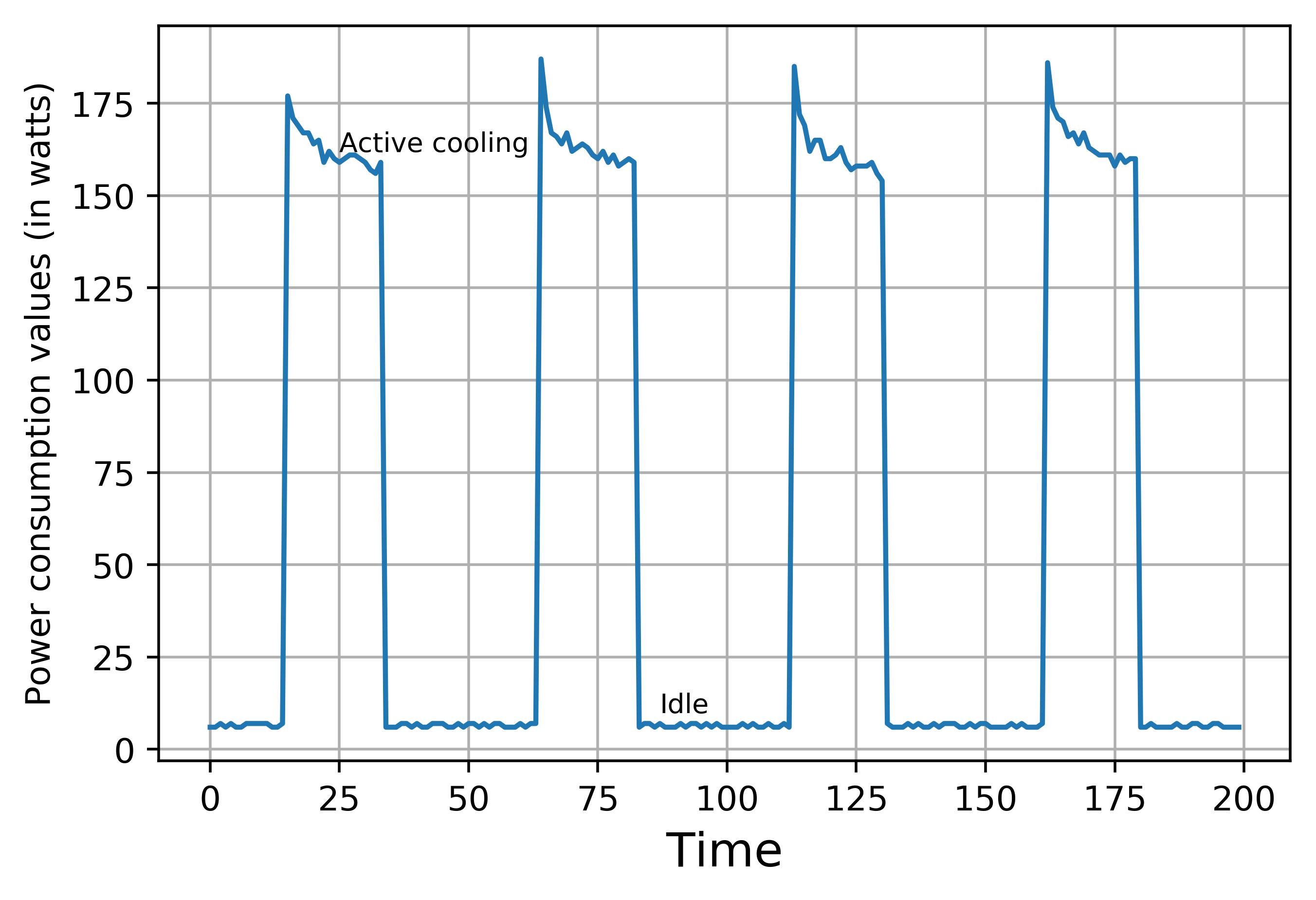
Figure 1. Energy consumption of a refrigerator. Horizontal and vertical axes correspond to time (seconds) and energy consumption (Watts), respectively. The energy consumption at active cooling and idle operation modes are shown. This figure shows that there exists pattern in energy consumption of appliances.

3.1. Powerlet Based Energy Disaggregation (PED)

PED introduced the concept of powerlets for energy disaggregation. It solves the problem by breaking the task into two phases, extracting the energy consumption pattern of each device and performing the actual disaggregation task among the extracted energy consumption patterns.

The operation modes of a device refer to the various modes in which it can operate based on the energy that it consumes. For example, a microwave can operate in operation modes such as defrost, heat with high power or low power or switched off state. The training phase of PED assumes that each device’s operation mode can be mapped to a vector of length $w$, referred to as powerlet, which represents the energy consumption pattern in that operation mode.

To find the powerlets of a device $i$, the energy consumption of the device in time interval $[t,t+w-1]$ is represented by a $w$-dimensional vector, $\boldsymbol{y}_{i}(t)$, where $t\in\{1,2,\ldots,T-w+1\}$. Powerlets for device $i$ are selected from the set of vectors $\mathcal{V}=\{\boldsymbol{y}_{i}(t),\forall t\in\{1,2,\ldots T-w+1\}\}$, using a variant of the DS3 algorithm for sequential data (Elhamifar et al., 2016). Let subdictionary $\boldsymbol{B}_{i}\in R^{w\times N_{i}}$ consists of the powerlets of device $i$, represented by a matrix whose columns are the powerlets and $N_{i}$ is the number of powerlets of device $i$. The dictionary, $\boldsymbol{B}\in R^{w\times N}$ where $N=\sum_{i=1}^{L}N_{i}$ is the set of subdictionaries of all the devices in the house and is obtained by concatenating the subdictionaries of all the devices, i.e.,

(1) $$\boldsymbol{B}=[\boldsymbol{B}_{1},\ldots,\boldsymbol{B}_{L}].$$

The vector $\boldsymbol{\bar{y}}(t)$ represents the aggregated energy consumption in time interval $[t,t+w-1$] i.e.,

(2) $$\boldsymbol{\bar{y}}(t)=[\bar{x}(t),\bar{x}(t+1),\ldots,\bar{x}(t+w-1)].$$

In its second phase, PED disaggregates the energy by solving the following optimization problem:

c(t) λρ(c(t)_t=1^T)+ ∑_t=1^T—— ¯y(t)-Bc(t)——_1 c_i(t)={0,1}^N_i 1^Tc_i(t) ≤1

where $\boldsymbol{c}(t)=[\boldsymbol{c}_{1}(t),\boldsymbol{c}_{2}(t),\ldots,\boldsymbol{c}_{L}(t)]\in\mathbb{R}^{N}$, $\boldsymbol{c}_{i}(t)\in\mathbb{R}^{N_{i}}$ is the coefficient of the powerlets of device $i$, $\lambda$ is a regularization parameter, and $\rho({\boldsymbol{c}(t)}_{t=1}^{T})$ indicates the penalty associated with the priors such as device-sparsity, knowledge about devices that do or do not work together, and temporal consistency of the disaggregation. The first constraint enforces the selection or not of a powerlet and the second constraint is used to ensure that at most one powerlet is selected for every device.

However, PED does not take into account the concurrent operation modes of devices within the time window $w$. The co-occurrence prior in PED only considers the devices which are used together or which are not used together. Instead, certain devices tend to be used concurrently at specific operation modes, which arises when certain tasks are performed.

3.2. Recursive dictionary learning for energy disaggregation

Deep Sparse Coding based Recursive Disaggregation Model
(DSCRDM) (Dong et al., 2013) exploits a tree structure for the problem of energy disaggregation, such that, at a particular level, one of the nodes contains one device and the other contains the rest. That device is separated from the remainder which minimizes the disaggregation error on the training set. DSCRDM is based on Discriminative Disaggregation Sparse Coding (Kolter et al., 2010) (DDSC) to find the dictionary of each appliance. DDSC models the entire energy consumption of each device as a sparse linear combination of the atoms of an unknown dictionary.

(a) Energy consumption of stove

(b) Energy consumption of refrigerator

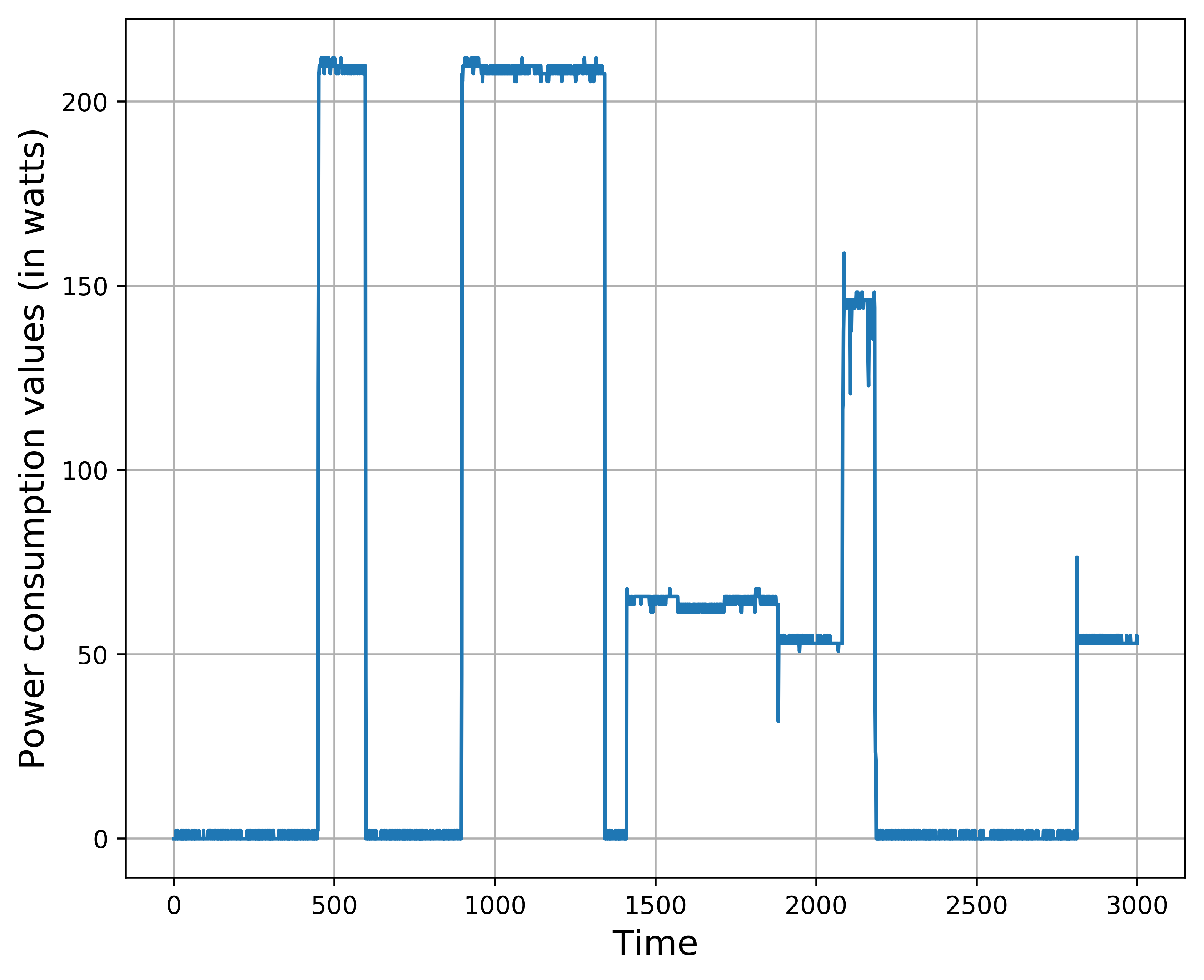
(c) Energy consumption of air exhaust

Figure 2. Illustration of devices having a similar energy consumption value. Both stove and refrigerator show a pattern where they tend to operate at 160W. The prior approaches may fail to distinguish between the power consumption of the two devices. We can resolve this by using the fact that the air exhaust is on whenever the stove is in use.

However, the dictionary atoms used in DDSC are arbitrary vectors which do not correspond to the energy consumption pattern of specific operation modes of the device. This degrades the disaggregation performance (Elhamifar and Sastry, 2015). Moreover, DSCRDM solves a non-convex problem to find the best split at each node which increases the computational complexity of training the decomposition structure.

4. Proposed Method

Similar to PED, we follow a two-step procedure for energy disaggregation. Firstly, we learn powerlets of different subsets of devices and the decomposition structure using the training dataset. Then we decode the aggregated energy consumption among the learned dictionary atoms at each level of the decomposition structure following an optimization scheme similar to PED. In this section, we first provide the motivation for our method followed by the framework we developed for energy disaggregation.

4.1. Motivation

The prior approaches for energy disaggregation face the common challenge of disaggregating energy of similar power consuming devices. For example, in Figure  2 both stove and refrigerator consume similar power. However, we observe that the air exhaust is usually on when the stove is used. Thus, for performing disaggregation we can consider the aggregated power consumption of air exhaust and stove as they have different power consumption pattern compared to the refrigerator alone. Grouping devices into sets and then performing disaggregation can help in distinguishing two similar power consuming devices. Motivated by this, we develop device decomposition methods to find the sequence in which energy is to be disaggregated.

Another fact to consider is that devices do not just merely co-occur but they co-occur at specific operation modes for performing one task and for another task they can co-occur at different modes. For example, when heating food, a person will start by opening the refrigerator to get the food item, which can potentially transition the fridge to an active cooling operation mode. Then the person puts the item in the microwave and switches it on. Thus, the transition of operation modes of the two devices tends to occur simultaneously. After switching the microwave on, the person puts the left out food back in the fridge which again changes the operation mode of the fridge. However, when a dish is being cooked, some other appliance in the kitchen can be used along with the microwave and fridge. Thus, a set of devices are used at specific modes, for certain tasks (food heating), whereas for other tasks (cooking), another set of devices are used simultaneously.

To summarize, it is important to group devices into sets and then perform disaggregation. Additionally, the co-occurence of devices is not specific to two devices merely operating together but the operation modes at which they co-occur is also important.

4.2. Learning powerlets

A powerlet is a vector of length $w$, which is used as a representative for a specific operation mode of a device. In order to find the powerlets, we select representatives among the set of vectors $\mathcal{V}=\{\boldsymbol{y}_{i}(t),\forall t\in\{1,2,\ldots T-w+1\}\}$, where $\boldsymbol{y}_{i}(t)$ is the energy consumption of the device during the time interval $[t,t+w-1]$. The DS3 algorithm employed in PED has high storage and computational complexity (Mavrokefalidis et al., 2016). A simpler clustering based method (Tosic and Frossard, 2011) can be used for selecting the representatives among the set of vectors. Specifically, we use $k$-medoid algorithm because both $k$-medoid and DS3 select representatives from the data to be clustered.

4.3. Learning dictionary and device decomposition structure

We create the device decomposition structure by decomposing the device set recursively into two equal halves (or one half with one device more than the other if the number of devices is odd) until only one device remains. This creates a binary tree structure containing sets of devices at every node. We choose to use binary tree as device decomposition structure because of its simplicity. For understanding purpose, we define a pseudo device as a hypothetical device whose energy consumption is the same as the aggregated energy consumption of the devices in the set, i.e., energy consumption of a pseudo device at time $t$, $x_{\rho}(t)$ is calculated as,

(3) $$x_{\rho}(t)=\sum_{i\in\mathcal{S}}x_{i}(t).$$

We extract the powerlets of the pseudo devices at each node. If devices in the set co-occur at a specific operation mode then the representative power consumption of that operation mode is one among the extracted representatives. We perform energy decomposition in a recursive manner, starting from the root node and disaggregating the aggregated energy assigned at every node between its two children. Figure 3 shows an example of the device decomposition structure.

In order to maximize the accuracy of decomposing the energy signal, we focus on making the powerlets of devices used for disaggregation as dissimilar as possible. A key parameter for constructing the device decomposition structure is the method that is used to partition the set of devices at each node of the tree.

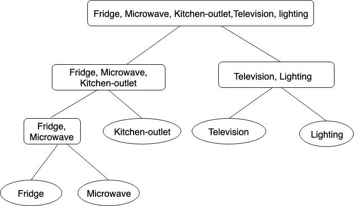
Figure 3. An example of binary tree structure of a particular house.

4.3.1. Greedy based Device Decomposition Method (GDDM):

This approach splits the set of devices into two groups by maximizing the dissimilarity between powerlets at each level.

Let $S_{1}$ and $S_{2}$ be the two subsets of devices created from the set of devices. Let $B_{1}$ and $B_{2}$ be the powerlets for these two pseudo devices. Dissimilarity of $S_{1}$ and $S_{2}$ is the distance between the pair of closest powerlets, one from each of the pseudo device, which is defined as,

(4) $$dissimilarity(S_{1},S_{2})=\min_{p,q}||\boldsymbol{B}_{1p}-\boldsymbol{B}_{2q}||_{1},$$

Since the disaggregation is performed using the powerlets of the pseudo devices, we want the resultant powerlets to be as dissimilar as possible. Hence, we maximize the dissimilarity between the two pseudo devices. We explore two different ways of splitting the device set greedily.
Equi-sized partition: To find equi-sized partitions, we start by randomly dividing the device set equally among the two nodes (or with one node having one more device than the other if the number of devices in the node is odd). We find a device, $d_{1}$ from the first node, which when moved to the second node leads to the maximum increase in the dissimilarity between the resultant pseudo devices. Similarly we find a device, $d_{2}$, from the resultant second node which when moved to the first node increases the dissimilarity between the resultant pseudo devices. We then move $d_{1}$ to the second node and $d_{2}$ to the first. We repeat this step until no such device is found which when moved increases the dissimilarity between the pseudo devices. Algorithm 1 describes how equi-sized partition is performed using GDDM.

Input: $S:$ The set of devices to be partitioned
	1begin
	2 $l\leftarrow$number of devices in $\mathcal{S}$
	3 Iterate until $d_{1}$ or $d_{2}$ is NULL:
	4  $\mathcal{S}_{1}\leftarrow\text{$l$/2 randomly selected devices}\in\mathcal{S}.$
	5  $\mathcal{S}_{2}\leftarrow\mathcal{S}\setminus\mathcal{S}_{1}$
	6  $d_{1}\leftarrow split(\mathcal{S}_{1},\mathcal{S}_{2})$
	7  $d_{2}\leftarrow split(\mathcal{S}_{2}\cup d_{1},\mathcal{S}_{1}\setminus d_{1})$
	8  $\mathcal{S}_{1}\leftarrow\mathcal{S}_{1}\cup d_{2}$
	9  $\mathcal{S}_{2}\leftarrow\mathcal{S}_{2}\cup d_{1}$
	10 Return $\mathcal{S}_{1},\mathcal{S}_{2}$

Alg. 1 Greedy based Maximizing Inter-set Dissimilarity Method (Equi-sized Partition)

Procedure: split($\mathcal{S}_{1}$, $\mathcal{S}_{2}$)
Input: $S:$ The set of devices to be partitioned
	1begin
	2 for $i\in\mathcal{S}_{1}$:
	3  $\boldsymbol{B}_{\rho}^{1}\leftarrow$ Powerlets of pseudo device $\mathcal{S}_{1}\setminus i$
	4  $\boldsymbol{B}_{\rho}^{2}\leftarrow$ Powerlets of $\mathcal{S}_{2}\cup i$
	5  CM(i)= $\min_{p,q}||\boldsymbol{B}_{{\rho}^{2}p}-\boldsymbol{B}_{{\rho}^{1}q}||_{1}$
	6 $d\leftarrow\max_{i}$ CM(i)
	7 $B_{S_{1}}\leftarrow$ powerlets of pseduo device $\mathcal{S}_{1}$
	8 $B_{S_{2}}\leftarrow$ powerlets of pseduo device $\mathcal{S}_{2}$
	9 CM(d) $>\min_{p,q}||B_{{S_{1}}p}-B_{{S_{2}}q}||$:
	10  Return NULL
	11 else:
	12  Return $d$

1-vs-rest partition: 1-vs-rest partitioning refers to the partitioning of a set of devices such that one of the subsets contains one device and the other contains the rest. For 1-vs-rest partitioning, we find a device $d$ such that its powerlets are most dissimilar to the powerlets of the pseudo device created by the remainder devices in the set. We then create two subsets - one containing the device $d$ and the other containing the rest. This step is repeated recursively until only one device is the left in the subset. Algorithm 2 describes 1-vs-rest partitioning using greedy mechanism.

Input: $S:$ The set of devices to be partitioned
	1begin
	2 for $d\subset\mathcal{S}$
	3  $\boldsymbol{B}_{d}\leftarrow$ Powerlets of device $d$
	4  $\boldsymbol{B}_{\rho}\leftarrow$ Powerlets of $\mathcal{S}\setminus d$
	5  $CM(d)=\min_{p,q}||\boldsymbol{B}_{{\rho}p}-\boldsymbol{B}_{{d}q}||_{1}$
	6 Return $\text{device}={\textrm{argmax}}_{i}CM(i)$

Alg. 2 Greedy based Device Decomposition Method (1-vs-rest)

4.3.2. Dynamic Programming based Device Decomposition Method (DPDDM):

In case of GDDM, we split a set of devices such that the dissimilarity between the powerlets of the pseudo devices corresponding to the children node can be maximized. Sometimes, splitting of devices to maximize the dissimilarity of only the resulting pseudo devices can result in children nodes containing devices with similar powerlets. For example, consider a house with devices $d_{1}$, $d_{2}$, and $d_{3}$, such that $d_{1}$ and $d_{2}$ have similar power consumption. Greedy based methods can result in a decomposition structure that it predicts the power consumption of $d_{3}$ followed by $d_{1}$ and $d_{2}$. Since it is difficult to distinguish the consumption pattern of $d_{1}$ and $d_{2}$, disaggregating energy between them can lead to error. However, DPDDM tries to find the optimal decomposition structure to address this limitation. The split is made by taking into consideration the overall dissimilarity between the powerlets that construct dictionary after any split. In DPDDM, we maximize the following objective function to find the decomposition structure,

(5) $$\sum_{\rho=1}^{N}|{\mathcal{S_{\rho}}}|^{\alpha}\min_{p,q}||\boldsymbol{B}^{1}_{\rho p}-\boldsymbol{B}^{2}_{\rho q}||_{1},$$

where $N$ is the total number of non-terminal nodes in the binary tree structure, $\mathcal{S}_{\rho}$ is the device set corresponding to the node $\rho$, $\boldsymbol{B}^{1}_{\rho}$ and $\boldsymbol{B}^{2}_{\rho}$ correspond to the subdictionaries of the pseudo devices of the left and right child of the node $\rho$, respectively, and $\alpha$ is a tunable parameter. Note that Equation (6) is a weighted combination of dissimilarity of powerlets used for disaggregation at all the levels in the decomposition structure. Since an error made in the top nodes of the decomposition structure propagates down the tree, we assign more weight to dissimilarity between powerlets of pseudo devices occurring in the top nodes than the bottom ones. The tree that gives the maximum value of the objective function is selected as the decomposition structure. To optimize the above objective function, we use the following recurrence relation while splitting the nodes,

(6) $$C_{\mathcal{S}}=\max_{{\mathcal{P}},|{\mathcal{P}}|={{|{\mathcal{S}}|}/2}}C_{\mathcal{P}}+C_{\mathcal{S}/\mathcal{P}}+|{\mathcal{S}}|^{\alpha}\min_{{p},{q}}||\boldsymbol{B}^{1}_{\rho p}-\boldsymbol{B}^{2}_{\rho q}||_{1},$$

where $C_{\mathcal{S}}$ is the optimum cost of the tree rooted at the node corresponding to device set $\mathcal{S}$, $B_{\rho}^{1}$ is the subdictionary of the pseudo device of $\mathcal{P}$ and $B_{\rho}^{2}$ is the subdictionary of the pseudo device of $\mathcal{S}/\mathcal{P}$. Algorithm 3 describes Dynamic Programming based Maximizing Inter-set Dissimilarity method.

Input: $S:$ The set of devices to be partitioned
	1begin
	2 for $\mathcal{P}\subset\mathcal{S}$ such that $|\mathcal{P}|=|\mathcal{S}|/2$:
	3  $\boldsymbol{B}_{\rho}^{1}\leftarrow$ Powerlets of pseudo device $\mathcal{P}$
	4  $\boldsymbol{B}_{\rho}^{2}\leftarrow$ Powerlets of $\mathcal{S}\setminus\mathcal{P}$
	5  $C_{\mathcal{S}}^{1}=$ DPDDM($\mathcal{P}$)
	6  $C_{S}^{2}=$ DPDDM($\mathcal{S}\setminus\mathcal{P}$)
	7  $C_{\mathcal{P}}=C_{\mathcal{S}}^{1}+C_{\mathcal{S}}^{2}$
$+|\mathcal{S}|^{\alpha}|\min_{p,q}||\boldsymbol{B}^{2}_{{\rho}p}-\boldsymbol{B}^{1}_{{\rho}q}||_{1}$
	8 $\mathcal{Q}={\textrm{argmax}}_{\mathcal{P}}C_{\mathcal{P}}$
	9 Return $\mathcal{Q}$, $\mathcal{S}\setminus\mathcal{Q}$

Alg. 3 Dynamic Programming based Device Decomposition Method (DPDDM)

4.4. Decomposing the energy signal

In order to disaggregate the energy, we start from the root node containing all the devices and approximate the aggregated energy consumption of the devices that belong to the child nodes. This step is performed recursively until we reach the leaf nodes which contain only one device. Thus, we modify the entire task of decomposing the energy signal into a recursive task. Note that, this is not the same as expressing Equation (3) recursively because the dictionaries involved in performing the disaggregation at each recursion is derived from the powerlets of the corresponding pseudo devices. Specifically, at every node, $\rho$, of the tree, the dictionary, $\boldsymbol{B}_{\rho}$ to be used for disaggregating the energy consumption is obtained by concatenating the subdictionaries of the pseudo devices of its two children, i.e., $B_{\rho}=[B^{1}_{\rho},B^{2}_{\rho}]$. Since a (pseudo) device can be operating in one of the operation modes, we select exactly one powerlet from the dictionary of the powerlets for every (pseudo) device. We solve the following optimization problem to obtain the energy consumption of the (pseudo) devices at every step:

c(t) ∑_t=1^T——(¯y_ρ(t)-B_ρc(t))——_2 c_i(t)={0,1}^N_i 1^Tc_i(t) = 1,

where $\boldsymbol{\bar{y}}_{\rho}(t)$ is the aggregated energy consumption of the devices that belong to node $\rho$. The last two constraints ensure the selection of exactly one powerlet per device.

Using decomposition structure for performing disaggregation of energy signal provides speedup as the time complexity of solving the non convex problem using standard solvers is exponential in the number of devices, $k$. By decomposing the problem into recursive, independent subproblems with less number of variables at each optimization, we reduce the time complexity to linear with respect to number of devices.

To solve Equation (8) we used ADMM based method as it is more computationally efficient (Park and Boyd, 2017) and scalable compared to integer programming based method used in PED. Note that, even though ADMM is scalabale with time complexity $\mathcal{O}(k^{3})$, our decomposition methods reduced the time complexity to $\mathcal{O}(k)$.

In order to reframe this problem in a general form, assume $\boldsymbol{c}(t)\in\mathbb{R}^{N}$ as $\boldsymbol{x}$, where $N$ is the sum of number of the powerlets of the two (pseudo) devices belonging to the child nodes, $\bar{\boldsymbol{y}}_{\rho}(t)$ as $\boldsymbol{b}$ and $\boldsymbol{B}_{\rho}$ as $\boldsymbol{A}$. All the linear constraints are combined such that matrix $\boldsymbol{P}\in\mathbb{R}^{2\times N}$ has $i$th row element, $e_{i}\in\mathbb{R}^{N}$ whose entries for the powerlets of pseudo (device) $i$ are one and the rest are zeros, $\boldsymbol{q}\in\mathbb{R}^{2}$ is a vector consisting of all ones.

x ——Ax-b——_2 x_i(x_i-1)=0 P^Tx = q.

Following the idea of SDP relaxation for integer programming problem (Park and Boyd, 2017), we can reformulate the above optimization as:

X, x Tr(A^TAX)-2*b^TAx diag(X) ≥x [ 1x^TxX ] ⪰0 P^Tx = q.

By introducing $\hat{\boldsymbol{X}}=\displaystyle\Big{[}\begin{array}[]{cc}1&\boldsymbol{x}^{T}\\ \boldsymbol{x}&\boldsymbol{X}\\ \end{array}\Big{]}$ we can represent Equation (10) in a more compact form as

^X

Tr(^A^X) ^X ⪰0 A(^X) = ~b,

where $\hat{\boldsymbol{A}}=\displaystyle{\Big{[}\begin{array}[]{cc}0&-\boldsymbol{b^{T}A}\\ -\boldsymbol{(b^{T}A)^{T}}&\boldsymbol{A^{T}A}\\ \end{array}\Big{]}}\in\mathbb{S}_{+}^{N+1},\tilde{\boldsymbol{b}}\in\mathbb{R}^{m}$ and ${\mathcal{A}}:\mathbb{S}_{+}^{N+1}\rightarrow\mathbb{R}^{m}$ is a linear map (Wen et al., 2010), $m$ is the number of equality constraints. In addition, we impose a non-negativity constraint on the matrix $\hat{\boldsymbol{X}}$. The final equation then becomes

^X

Tr(^A^X) ^X ⪰0 A(^X) = ~b,

where $\hat{\boldsymbol{A}}=\displaystyle{\Big{[}\begin{array}[]{cc}0&-\boldsymbol{b^{T}A}\\ -\boldsymbol{(b^{T}A)^{T}}&\boldsymbol{A^{T}A}\\ \end{array}\Big{]}}\in\mathbb{S}_{+}^{N+1},\tilde{\boldsymbol{b}}\in\mathbb{R}^{m}$ and ${\mathcal{A}}:\mathbb{S}_{+}^{N+1}\rightarrow\mathbb{R}^{m}$ is a linear map (Wen et al., 2010), $m$ is the number of equality constraints. In addition, we impose a non-negativity constraint on the matrix $\hat{\boldsymbol{X}}$. The final equation then becomes

^X

Tr(^A^X) ^X ⪰0, ^X ≥0 A (^X) = ~b.

To apply ADMM on Equation (11), we use Moreau-Yosida quadratic regularization  (Malick et al., 2009).

Lagrangian function for Equation (11) can be written as

$$\mathcal{L}_{\mu}=Tr(\hat{\boldsymbol{A}}\hat{\boldsymbol{X}})+\frac{1}{2\mu}{||\hat{\boldsymbol{X}}-\boldsymbol{S}||}_{F}^{2}+\lambda^{T}(\tilde{\boldsymbol{b}}-\mathcal{A}(\boldsymbol{X})\\ -Tr(\boldsymbol{W}^{T}\hat{\boldsymbol{X}})-Tr(\boldsymbol{P}^{T}\hat{\boldsymbol{X}}),$$

where $\lambda\geq 0,\ \boldsymbol{P}\succeq 0,\ ,\boldsymbol{W}\geq 0$ are dual variables and $\mu>0$ is a constant.

By taking the derivative of ${\mathcal{L}}_{\mu}$ and computing optimal value of $\hat{\boldsymbol{X}}$, one can derive the standard updates of ADMM solver.

After obtaining optimal, $\boldsymbol{X}^{\star}$ and $\boldsymbol{x}^{\star}$ from $\hat{\boldsymbol{X}}$, we use randomized rounding (Park and Boyd, 2017) for finding an approximate solution, $\boldsymbol{x}^{opt}$ to our original problem which minimizes the optimization function of Equation (12). We randomly sample $\boldsymbol{z}$ from ${\mathcal{N}}(\boldsymbol{x}^{\star},\boldsymbol{X}^{\star}-\boldsymbol{x}^{\star}\boldsymbol{x}^{\star T})$. After obtaining $\boldsymbol{z}$, we greedily change its values so that the constraint of selection of exactly one powerlet per device is met. After performing this random sampling for few iterations, we select the optimal $\boldsymbol{z}^{\star}$ that gives lowest value of objective function as $\boldsymbol{x}^{opt}$.

Since the results at various time instants are independent, we solve each integer quadratic problem sequentially.

5. Experimental Setup

5.1. Datasets

We evaluate our results on the publicly available Electricity Consumption & Occupancy (ECO)  (Beckel et al., 2014) and the UK Domestic Appliance-Level Electricity (UK-DALE)  (Kelly and Knottenbelt, 2015b) datasets.
ECO (Beckel et al., 2014): This dataset contains the energy consumption of 6 households and the average number of appliances in the households is 7. The data was collected over a span of 8 months. The meter readings is recorded at a frequency of 1 Hz. We sample the data so that the consecutive energy consumption readings are at an interval of one minute.
UK-DALE (Kelly and Knottenbelt, 2015b): This dataset monitors $5$ households and the recordings are available every $6$ second. In this dataset, there are varying number of devices from $6$ to $24$. We sample this data also so that the consecutive energy consumption readings are at an interval of one minute.
The ground truth data is the actual energy consumption of each appliance. We use the readings with mains label in the dataset as the aggregated power consumption value.

5.2. Evaluation Methodology and Performance Assessment Metrics

Approaches: We compare our methods with three other existing methods: PED (Elhamifar and Sastry, 2015), Seq2point (Zhang et al., 2018) and DSCRDM (Dong et al., 2013), which are described in section 3. DSCRDM applies its decomposition learning on DDSC which faces the challenges mentioned in Section 3.2. For fairest comparison of the decomposition structure learning techniques, we modify DSCRDM to use its method of structure learning on dictionary learned using PED and refer to the resulting method as Modified DSCRDM (MDSCRDM).
Metrics: We assess the performance of the different methods using three different metrics: macro-averaged $f$ score ($Mf$), micro-averaged $f$ score ($\mu f$) and Normalized Disaggregation Error (NDE) which were introduced in  (Kolter and Jaakkola, 2012).

We use True Positive (TP) as the portion of the predicted energy consumption of a device that it actually consumes, False Negative (FN) as the portion of the actual energy consumption that is not predicted and False Positive (FP) as the portion of predicted energy consumption that is not a part of the actual energy consumption. Since there is no notion of predicting non-consumption of energy, True Negative (TN) is 0.

(7) $$\text{TP}_{i,t}=\frac{\min(x_{i,t},\hat{x}_{i,t})}{\hat{x}_{i,t}},\text{ FP}_{i,t}=\frac{\min(0,\hat{x}_{i,t}-x_{i,t})}{\hat{x}_{i,t}},$$

(8) $$\text{FN}_{i,t}=\frac{\min(0,x_{i,t}-\hat{x}_{i,t})}{x_{i,t}},\text{TN}=0.$$

For $\mu f$ score, we define the precision and recall as:

(9) $$\mu Precision=\frac{\sum_{t=1}^{T}\sum_{i\in\mathcal{D}}\text{TP}_{i,t}}{\sum_{t=1}^{T}\sum_{i\in\mathcal{D}}(\text{TP}_{i,t}+\text{FP}_{i,t})}$$

(10) $$\mu Recall=\frac{\sum_{t=1}^{T}\sum_{i\in\mathcal{D}}\text{TP}_{i,t}}{\sum_{t=1}^{T}\sum_{i\in\mathcal{D}}(\text{TP}_{i,t}+\text{FN}_{i,t})}$$

For $Mf$ score, we define the precision and recall as:

(11) $$Precision_{i}=\frac{\sum_{t=1}^{T}\text{TP}_{i,t}}{\sum_{t=1}^{T}(\text{TP}_{i,t}+\text{FP}_{i,t})},$$

(12) $$Recall_{i}=\frac{\sum_{t=1}^{T}\text{TP}_{i,t}}{\sum_{t=1}^{T}(\text{TP}_{i,t}+\text{FN}_{i,t})}$$

(13) $$MPrecision=\frac{\sum_{i\in\mathcal{D}}Precision_{i}}{|\mathcal{D}|},$$

(14) $$MRecall=\frac{\sum_{i\in\mathcal{D}}Recall_{i}}{|\mathcal{D}|},$$

where, $\mathcal{D}$ is the set of devices in the house. The harmonic mean of $\mu$ and $M$ precision and recall gives $\mu$ and $M$ $f$ scores  (Tabatabaei et al., 2017), respectively.

The difference between the two $f$ scores is that the $Mf$ score gives equal weight to each device, whereas the $\mu f$ score tends to give higher importance to devices that consume high power.

We also use the popular metric, Normalized Disaggregation Error
(NDE) (Zhong et al., 2014).

(15) $$NDE=\frac{\sum_{i,t}(\hat{x}_{i,t}-x_{i,t})^{2}}{\sum x^{2}_{i,t}}$$

Model Training and Parameter Selection: We train each model using $80\%$ of the data with respect to time and test it on the rest. The parameters of the methods used are kept unchanged. We compute the performance of GDDM in terms of the $f$ scores and NDE averaged over all the houses of ECO and UK-Dale at different values $w\in\{5,15,25,35\}$ and $k\in\{20,40,60\}$. We find that $w=15$ gives the best performance for the method and for $w=15$, the best performance on the test data is obtained when $k$ is $40$. For our device decomposition methods we use $w=15$ and $k=40$.

For DPDDM, the weights associated with a node is calculated as $|\mathcal{S}|^{\alpha}$, where ${\mathcal{S}}$ is the set of devices belonging to the node. We try three different values of $\alpha[1,2,3]$ and find that $\alpha=2$ gives the best performance for all the metrics.

6. Results and Discussion

Table 2. The performance of GDDM_ADMM, GDDM_IP the houses of the UK-Dale dataset.

Method	$\mu f$	$Mf$	NDE
GDDM_IP	0.517	0.761	1.665
GDDM_ADMM	0.535	0.765	1.701

Table 3. The performance of device decomposition methods for all the house in the UK-Dale and ECO dataset. Both our methods DPDDM, GDDM (equi-sized) outperform the existing state-of-the-art methods. ^1,2,3

	UK-Dale				ECO
	$\mu f$	$Mf$	NDE		$\mu f$	$Mf$	NDE
GDDM (equi-sized)	0.535$\pm$0.168	0.765$\pm$0.038	1.701$\pm$0.884		0.473$\pm$0.139	0.741$\pm$0.070	1.018$\pm$0.617
PED	0.409$\pm$0.209	0.696$\pm$0.053	2.832$\pm$1.131		0.405$\pm$0.036	0.682$\pm$0.108	3.321$\pm$0.434
seq2point	0.432$\pm$0.300	0.681$\pm$0.108	1.753$\pm$1.445		0.338$\pm$0.079	0.639$\pm$0.015	2.488$\pm$0.195

• shown are mean$\pm$ standard deviation values.

• Bold numbers are the best performance for the corresponding metric.

• For $Mf$ and $\mu f$ measures higher values and for NDE lower values are better, respectively.

6.1. Comparison of optimization methods for decomposing the energy signal

PED uses standard integer programming solver MOSEK (CVX Research, 2012) for solving optimization functions with integer constraints as is the case in Equation (8). In order to validate that the improvement in the performance of the device decomposition methods is because of utilizing decomposition of device set scheme and not the optimization solver, we compare the results of GDDM with equi-sized partition with the integer programming solver (GDDM_IP) and GDDM with ADMM (GDDM_ADMM). The results are shown in Table 2 and none of the methods perform consistently better than the other. The discussion on solvers for integer convex quadratic problem also suggests that SDP formulation achieves a good optimal solution (Park and Boyd, 2017) comparable to standard integer programming solvers.

6.2. Comparison of device decomposition methods

Table 3 shows the performance of GDDM (1-vs-rest), GDDM (equi-sized partition), DPDDM, and MDSCRDM for dividing the devices at each node on the ECO and the UK-Dale datasets. From the results, we observe that the equi-sized partitioning methods (GDDM (with equi-sized) and DPDDM) perform better than the 1-vs-rest (MDSRDM and GDDM (1-vs-rest)) partitioning methods. We perform a paired t-test on the values of $f$ scores and NDE obtained for all the houses in both the datasets. For the null hypothesis that the results of GDDM (equi-sized partition) and MDSCRDM are derived from the same distribution, the resulting p-value (  0.01) shows that the difference is statistically significant. The same holds for results of GDDM (equi-sized partition) and GDDM (1-vs-rest partition).

Table 4. Per appliance performance comparison. This table shows how our method performs at predicting the power consumption of each appliance. Our method performs better for the appliances which consume most power in a household and are used frequently (Fridge and freezer).

	$\mu f$				$Mf$				NDE
Appliance	GDDM	PED	seq2point		GDDM	PED	seq2point		GDDM	PED	seq2point
Fridge	0.620	0.181	0.445		0.763	0.235	0.704		0.552	0.894	0.997
Dryer	0.426	0.149	0.447		0.653	0.246	0.607		1.005	1.029	1.093
Coffee Machine	0.037	0.001	0.027		0.835	0.945	0.085		1.896	1.354	1.003
Kettle	0.009	0.000	0.003		0.946	0.991	0.826		1.976	2.946	1.037
Washing Machine	0.001	0.004	0.005		0.844	0.941	0.738		0.999	1.644	1.237
PC	0.047	0.013	0.068		0.441	0.810	0.619		1.655	1.026	1.046
Freezer	0.542	0.174	0.273		0.714	0.423	0.593		0.926	0.980	5.879
Average	0.240	0.075	0.181		0.742	0.656	0.596		1.287	1.410	1.756

• Bold numbers are the best performance for the corresponding metric.

• For $Mf$ and $\mu f$ measures higher values and for NDE lower values are better, respectively.

6.3. Comparison with PED and Seq2point

Tables 3 shows the performance achieved by GDDM, Seq2point, and PED on the ECO and UK-Dale datasets. For ECO, GDDM improves average performance by $16.7\%$, $8.65\%$ and $69.3\%$ in terms of the $\mu f$, $Mf$ and NDE, respectively compared to PED. Compared to the seq2point method, we obtain an improvement of $39.9\%$, $15.9\%$ and $59.3\%$ in terms of the $\mu f$, $Mf$ and NDE, respectively. The improvements obtained by GDDM is statistically significant at confidence level of $1\%$. In comparison with PED, for UK-Dale, GDDM improved the performance by $30.8\%$, $10\%$ and $39.9\%$, in terms of $\mu f$, $Mf$ and NDE, respectively. Compared to seq2point method, GDDM achieved performance improvement of $23.8\%$, $12.3\%$, and $2.9\%$ in terms of $\mu f$, $Mf$ and NDE, respectively on UK-Dale. The paired t-test shows that the improvement in terms of $Mf$ and $\mu f$ is significant (pvalue $<0.02$) while the improvement on NDE is not.

Additionally, we compare the three methods on appliance level performance. Table 4 shows the performance of various methods on all the appliances of house 1 of the ECO dataset. We can see that our method GDDM performs better than the other methods for half the number devices in terms of $\mu f$. The $Mf$ score of PED method is better for $4$ devices compared to our method. In terms of NDE, our method performs better for $4$ devices compared to the other two methods. Additionally, our method shows better performance in terms of the overall average $\mu f$, $Mf$ and NDE than the other two.

6.4. Visualization of Device Decomposition Strucuture

In order to show the effectiveness of designing a decomposition structure for performing disaggregation, we visualize how disaggregation is performed on the $1$st household of the ECO dataset. Figure 4(a) shows the device decomposition structure used by our method for performing disaggregation. Note that even though appliances such as washing machine and fridge show similar power consumption values when active, they can be distinguished by our method as the powerlets of pseudo devices {PC, Dryer and washing machine} or {Fridge, Freezer, Kettle and coffee machine } are different. This is because in some cases the activation of fridge could co-occur with freezer or kettle. Thus, using decomposition structure helps in capturing the co-occurence of devices and improve the disaggregation performance for this house. Figure 4(b) visualizes the powerlets of different (pseudo) devices at each level.

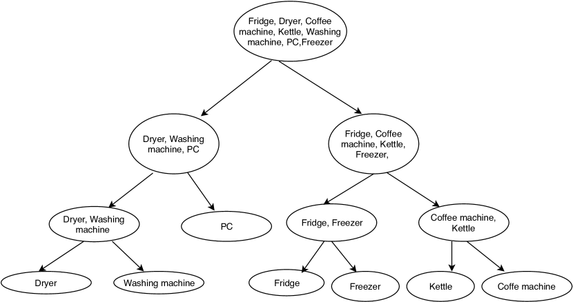
(a) Decomposition structure used for disaggregating the electricity consumption of House 1 in ECO dataset. The devices such as (Kettle, Coffee machine), which co-occur are discovered by our method and used for disambiguating similar power consuming devices.

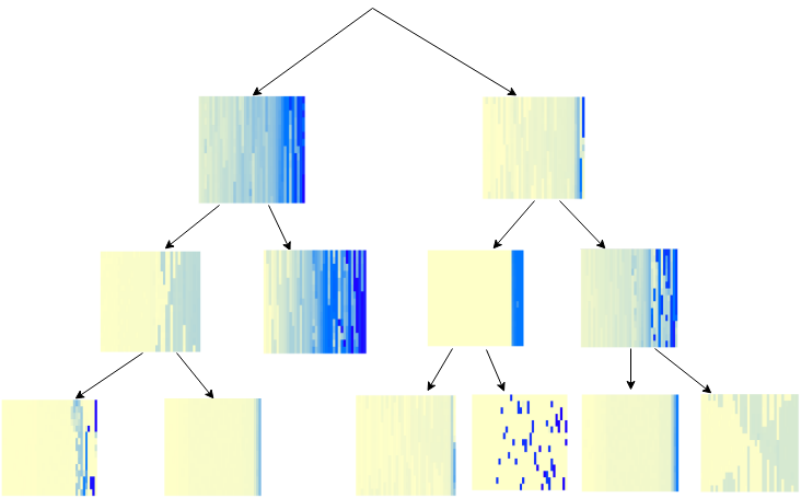
(b) Visualization of powerlets of the pseudo devices at each level of the device decomposition structure shown above.

Figure 4. Visualization of device decomposition structures.

Table 5. Training time (in minutes) of various methods for training house2 of UK Dale dataset.

GDDM	DPDDM	MDSCRDM	PED	seq2point
3.33	8.56	323.33	0.33	1735.45

6.5. Training Efficieny

Table 5 shows the training time taken by various methods using Intel Xeon E7 processor. PED takes the least time for training while seq2point takes the most. Our approaches take an order of magnitude less time to train as compared to MDSCRDM because MDSCRDM solves an optimization function at each level for splitting the device set while our methods use heuristics to find the best split.

7. Conclusion and Future work

In this paper, we improved the performance of the existing methods to obtain appliance level energy consumption from the aggregated energy of a house. Our methods leverage the fact that devices operate concurrently at specific operation modes. In order to capture the concurrent operating devices, we find the representatives of power consumption of sets of devices. We decompose the device set hierarchically to improve the performance of the task. We have empirically shown that device decomposition methods mostly outperform the state of the art methods on two real world data sets. The strength of our methods is that they are able to learn the devices that operate concurrently and use this knowledge to distinguish two similar energy consuming devices.

As part of future work, we plan to model the power consumption pattern of devices by including how the power consumption of device vary over time. Devices usually exhibit complex exponential decays or growth, bounded min-max, and cyclic patterns (Iyengar et al., 2016) of power consumption. This idea can be incorporated in extracting the powerlets. Additionally, a limitation of our model is that it is heavily dependent on the idea that devices in a house co-occur at some of their operation modes. However, if that is not the case, we can use simpler methods, such as PED. In future we plan to design a method to detect if some devices in the set go together and use our method to disaggregate energy only for those scenarios, otherwise use PED.

8. Acknowledgement

This work was supported in part by NSF (1447788, 1704074, 1757916, 1834251), Army Research Office (W911NF1810344), Intel Corp, and the Digital Technology Center at the University of Minnesota. Access to research and computing facilities was provided by the Digital Technology Center and the Minnesota Supercomputing Institute.

References

- (1)
- Attari et al. (2010) Shahzeen Z Attari, Michael L DeKay, Cliff I Davidson, and Wändi Bruine De Bruin. 2010. Public perceptions of energy consumption and savings. Proceedings of the National Academy of sciences 107, 37 (2010), 16054–16059.
- Batra et al. (2016) Nipun Batra, Amarjeet Singh, and Kamin Whitehouse. 2016. Gemello: Creating a detailed energy breakdown from just the monthly electricity bill. In Proceedings of the 22nd ACM SIGKDD International Conference on Knowledge Discovery and Data Mining. ACM, 431–440.
- Batra et al. (2017) Nipun Batra, Hongning Wang, Amarjeet Singh, and Kamin Whitehouse. 2017. Matrix Factorisation for Scalable Energy Breakdown.. In AAAI. 4467–4473.
- Beckel et al. (2014) Christian Beckel, Wilhelm Kleiminger, Romano Cicchetti, Thorsten Staake, and Silvia Santini. 2014. The ECO data set and the performance of non-intrusive load monitoring algorithms. In Proceedings of the 1st ACM Conference on Embedded Systems for Energy-Efficient Buildings. ACM, 80–89.
- Boyd et al. (2011) Stephen Boyd, Neal Parikh, Eric Chu, Borja Peleato, and Jonathan Eckstein. 2011. Distributed optimization and statistical learning via the alternating direction method of multipliers. Foundations and Trends® in Machine Learning 3, 1 (2011), 1–122.
- CVX Research (2012) Inc. CVX Research. 2012. CVX: Matlab Software for Disciplined Convex Programming, version 2.0. http://cvxr.com/cvx. (Aug. 2012).
- Dietz et al. (2009) Thomas Dietz, Gerald T Gardner, Jonathan Gilligan, Paul C Stern, and Michael P Vandenbergh. 2009. Household actions can provide a behavioral wedge to rapidly reduce US carbon emissions. Proceedings of the National Academy of Sciences 106, 44 (2009), 18452–18456.
- Dong et al. (2013) Haili Dong, Bingsheng Wang, and Chang-Tien Lu. 2013. Deep Sparse Coding based Recursive Disaggregation Model for Water Conservation.
- Elhamifar et al. (2016) Ehsan Elhamifar, Guillermo Sapiro, and S Shankar Sastry. 2016. Dissimilarity-based sparse subset selection. IEEE transactions on pattern analysis and machine intelligence 38, 11 (2016), 2182–2197.
- Elhamifar and Sastry (2015) Ehsan Elhamifar and Shankar Sastry. 2015. Energy Disaggregation via Learning Powerlets and Sparse Coding.. In AAAI. 629–635.
- Froehlich et al. (2011) Jon Froehlich, Eric Larson, Sidhant Gupta, Gabe Cohn, Matthew Reynolds, and Shwetak Patel. 2011. Disaggregated end-use energy sensing for the smart grid. IEEE Pervasive Computing 10, 1 (2011), 28–39.
- Gardner and Stern (2008) Gerald T Gardner and Paul C Stern. 2008. The short list: The most effective actions US households can take to curb climate change. Environment: science and policy for sustainable development 50, 5 (2008), 12–25.
- Hart (1992) George William Hart. 1992. Nonintrusive appliance load monitoring. Proc. IEEE 80, 12 (1992), 1870–1891.
- Iyengar et al. (2016) Srinivasan Iyengar, David Irwin, and Prashant Shenoy. 2016. Non-intrusive model derivation: automated modeling of residential electrical loads. In Proceedings of the Seventh International Conference on Future Energy Systems. ACM, 2.
- Kelly and Knottenbelt (2015a) Jack Kelly and William Knottenbelt. 2015a. Neural nilm: Deep neural networks applied to energy disaggregation. In Proceedings of the 2nd ACM International Conference on Embedded Systems for Energy-Efficient Built Environments. ACM, 55–64.
- Kelly and Knottenbelt (2015b) Jack Kelly and William Knottenbelt. 2015b. The UK-DALE dataset, domestic appliance-level electricity demand and whole-house demand from five UK homes. Scientific data 2 (2015), 150007.
- Kim et al. (2011) Hyungsul Kim, Manish Marwah, Martin Arlitt, Geoff Lyon, and Jiawei Han. 2011. Unsupervised disaggregation of low frequency power measurements. In Proceedings of the 2011 SIAM International Conference on Data Mining. SIAM, 747–758.
- Kolter et al. (2010) J Zico Kolter, Siddharth Batra, and Andrew Y Ng. 2010. Energy disaggregation via discriminative sparse coding. In Advances in Neural Information Processing Systems. 1153–1161.
- Kolter and Jaakkola (2012) J Zico Kolter and Tommi Jaakkola. 2012. Approximate inference in additive factorial hmms with application to energy disaggregation. In Artificial Intelligence and Statistics. 1472–1482.
- Malick et al. (2009) Jérôme Malick, Janez Povh, Franz Rendl, and Angelika Wiegele. 2009. Regularization methods for semidefinite programming. SIAM Journal on Optimization 20, 1 (2009), 336–356.
- Mavrokefalidis et al. (2016) Christos Mavrokefalidis, Dimitris Ampeliotis, Evangelos Vlachos, Kostas Berberidis, and E Varvarigos. 2016. Supervised energy disaggregation using dictionary—based modelling of appliance states. In PES Innovative Smart Grid Technologies Conference Europe (ISGT-Europe), 2016 IEEE. IEEE, 1–6.
- Park and Boyd (2017) Jaehyun Park and Stephen Boyd. 2017. A semidefinite programming method for integer convex quadratic minimization. Optimization Letters (2017), 1–20.
- Rahimpour et al. (2017) Alireza Rahimpour, Hairong Qi, David Fugate, and Teja Kuruganti. 2017. Non-intrusive energy disaggregation using non-negative matrix factorization with sum-to-k constraint. IEEE Transactions on Power Systems 32, 6 (2017), 4430–4441.
- Shaloudegi et al. (2016) Kiarash Shaloudegi, András György, Csaba Szepesvári, and Wilsun Xu. 2016. SDP relaxation with randomized rounding for energy disaggregation. In Advances in Neural Information Processing Systems. 4978–4986.
- Szydlowski (1993) RF Szydlowski. 1993. Advanced metering techniques. Technical Report. Pacific Northwest Lab., Richland, WA (United States).
- Tabatabaei et al. (2017) Seyed Mostafa Tabatabaei, Scott Dick, and Wilsun Xu. 2017. Toward non-intrusive load monitoring via multi-label classification. IEEE Transactions on Smart Grid 8, 1 (2017), 26–40.
- Tomkins et al. (2017) Sabina Tomkins, Jay Pujara, and Lise Getoor. 2017. Disambiguating Energy Disaggregation: A Collective Probabilistic Approach. (08 2017), 2857–2863.
- Tosic and Frossard (2011) Ivana Tosic and Pascal Frossard. 2011. Dictionary learning. IEEE Signal Processing Magazine 28, 2 (2011), 27–38.
- Wen et al. (2010) Zaiwen Wen, Donald Goldfarb, and Wotao Yin. 2010. Alternating direction augmented Lagrangian methods for semidefinite programming. Mathematical Programming Computation 2, 3 (2010), 203–230.
- Zhang et al. (2018) Chaoyun Zhang, Mingjun Zhong, Zongzuo Wang, Nigel Goddard, and Charles Sutton. 2018. Sequence-to-point learning with neural networks for non-intrusive load monitoring. In Thirty-Second AAAI Conference on Artificial Intelligence.
- Zhong et al. (2014) Mingjun Zhong, Nigel Goddard, and Charles Sutton. 2014. Signal aggregate constraints in additive factorial HMMs, with application to energy disaggregation. In Advances in Neural Information Processing Systems. 3590–3598.