Electromagnetic Formalism of the Propagation and Amplification of Light

Abstract

In this work, we present a simplified but comprehensive derivation of all the key concepts and main results concerning light pulse propagation in dielectric media, including a brief extension to the case of active media and laser oscillation. Clarifications of the concepts of slow light and “superluminality” are provided, and a detailed discussion on the concept of transform-limited pulses is also included in the Appendix.

1 Introduction

In this article we present a route that starts from basic electromagnetism concepts and leads to the development of the essential theory of various basic devices and subsystems widely employed in telecommunication photonics.

Of course, such derivations can be found by the hundreds in the literature, but, in our opinion, they are rarely self-contained and are often hasty, in some sense “improvised”, with the result that it is difficult for the reader to recognize the key ideas beyond what is simply accessory. Sometimes, the routine and careless use of certain formalisms (which, on some occasions, are not even really well-understood) further obscures the conceptualization process.

Here we present the key concepts in the simplest possible way, but in a rigorous fashion as to the logical order of the development and the connections between the successive results, both from the field of electromagnetism in dielectrics and from signal theory. Most of all, we want to avoid the “scattered” nature of the fragmented presentations referred to above.

The required electromagnetic theory is presented in Section 2. We can, and will, limit ourselves to the simplest case: the propagation of plane waves in homogeneous, infinite dielectrics. Additionally, the dielectrics will be, at this time, linear and isotropic. With this background, Section 3 studies the transmission of signals in dielectrics without any mention to waveguiding structures; in our presentation, all the key ideas will be introduced and clarified in the simple frame of non-guided, plane wave propagation. The great advantage of this approach is that the fundamental concepts thus acquired can be very easily generalized, at a later stage, to more realistic situations.

2 Electromagnetism of optical waves

In this section we will mainly be concerned with the derivation of the wave equation in linear dispersive dielectrics. A few general, simple results directly following from it are also presented.

2.1 Linear response of an (isotropic) dielectric

In their fundamental form, the Maxwell equations read as follows:

$$\ \nabla\cdot\mbox{\boldmath$\mathcal{E}$}(\boldsymbol{r},t) =\frac{\rho(\boldsymbol{r},t)}{\epsilon_{0}}$$ (1)

$$\nabla\cdot\mbox{\boldmath$\mathcal{B}$}(\boldsymbol{r},t) =0$$ (2)

$$\nabla\times\mbox{\boldmath$\mathcal{E}$}(\boldsymbol{r},t) =-\frac{\partial}{\partial\,t}\mbox{\boldmath$\mathcal{B}$}(\boldsymbol{r},t)$$ (3)

$$c^{2}\nabla\times\mbox{\boldmath$\mathcal{B}$}(\boldsymbol{r},t) =\frac{\mbox{\boldmath$\mathcal{J}$}(\boldsymbol{r},t)}{\epsilon_{0}}+\frac{\partial}{\partial\,t}\mbox{\boldmath$\mathcal{E}$}(\boldsymbol{r},t).$$ (4)

The adjective “fundamental” means two things here:

(a) Only two fields, $\mathcal{E}$ (electric field strength) and $\mathcal{B}$ (magnetic induction), appear in the equations. These are considered to be the genuine fields which describe the electromagnetism in nature. The electric displacement field $\mathcal{D}$, often included in the set of Maxwell equations on the same footing as $\mathcal{E}$, is an “artificial” field introduced as an aid to describe the macroscopic response of the dielectric materials to the electromagnetic (EM) fields. In many cases, the material response leads to a surprisingly simple (albeit approximate) linear relation between both fields: $\mbox{\boldmath$\mathcal{D}$}(t)=\varepsilon\mbox{\boldmath$\mathcal{E}$}(t)$, as remarked in the Introduction. Under these circumstances, all the effects of the material response can be trivially accounted for, with very good accuracy, by a mere constant $\varepsilon$ (the dielectric permittivity or dielectric constant of the material). However, this will frequently not be the case in Photonics. On the other hand, since the dielectrics materials we will be concerned with are diamagnetic, a simple linear relation between $\mathcal{B}$ and the so-called magnetic induction, $\mbox{\boldmath$\mathcal{H}$},$ will be generally valid in the situations studied here:

$$\mbox{\boldmath$\mathcal{B}$}(t)=\mu\mbox{\boldmath$\mathcal{H}$}(t),$$ (5)

with $\mu$ the magnetic permeability. We will thus not need to dwell on any magnetic properties of matter, and either $\mathcal{B}$ or $\mathcal{H}$ will be used at our convenience. Moreover, almost all materials of interest in Photonics are diamagnetic or paramagnetic, so the magnetic permeability can be taken as that of the vacuum in all cases: $\mu\simeq\mu_{0}=4\pi\times 10^{-7}$ N$\times$A${}^{-2}.$

(b) $\rho(\boldsymbol{r},t)$ in (1) is the total change density in space, including not only the “free” charges (which give rise to the electric conduction current), but also the bound charges of the atoms which make up the dielectric. This is,

$$\rho(\boldsymbol{r},t)=\rho_{d}(\boldsymbol{r},t)+\rho_{f}(\boldsymbol{r},t),$$ (6)

where $d$ and $f$ stand for “dielectric” and “free”, respectively. Likewise, $\mathcal{J}$ in (4) is given by

$$\mbox{\boldmath$\mathcal{J}$}(\boldsymbol{r},t)=\mbox{\boldmath$\mathcal{J}$}{}_{d}(\boldsymbol{r},t)+\mbox{\boldmath$\mathcal{J}$}{}_{f}(\boldsymbol{r},t),$$ (7)

where $\mbox{\boldmath$\mathcal{J}$}{}_{d},$ the “dielectric current” originated from the temporal variation of the dielectric charge density, adds to the free conduction current $\mbox{\boldmath$\mathcal{J}$}{}_{f}.$The key issue will be to obtain the form of $\rho_{d}$ (and $\mbox{\boldmath$\mathcal{J}$}{}_{d}$), but, as long as a specific model for the dielectric interaction has not been chosen, eqs. (1)–(4) remain general.

The wave equation is the equation for one field only, whether $\mathcal{E}$ or $\mbox{\boldmath$\mathcal{B}$}.$ In our context, the electric field is almost always chosen and the derivation of the wave equation is straightforward. Taking the curl of (3), replacing $\nabla\times\mbox{\boldmath$\mathcal{B}$}$ in favour of $\mathcal{E}$ by means of (4), applying the general vector relation $\nabla\times[\nabla\times\boldsymbol{F}]=\nabla(\nabla\cdot\boldsymbol{F})-\nabla^{2}\boldsymbol{F,}$ and making use of eq. (1), the following equation is obtained:

$$\nabla^{2}\mbox{\boldmath$\mathcal{E}$}(\boldsymbol{r},t)-\dfrac{1}{c^{2}}\frac{\partial^{2}}{\partial\,t^{2}}\mbox{\boldmath$\mathcal{E}$}(\boldsymbol{r},t) =\dfrac{1}{\varepsilon_{0}}\nabla\rho_{d}(\boldsymbol{r},t)+\dfrac{1}{\varepsilon_{0}c^{2}}\frac{\partial}{\partial\,t}\mbox{\boldmath$\mathcal{J}$}{}_{d}(\boldsymbol{r},t)$$ (8)

{no free charges}.

It has also been assumed in (8) that the dielectric is a perfect isolator; therefore $\rho_{f}=0$ and $\mbox{\boldmath$\mathcal{J}$}{}_{f}=\mathbf{0}.$

We will first consider the vacuum as the medium where the propagation takes place. Then, $\rho_{d}=0$ and $\mbox{\boldmath$\mathcal{J}$}{}_{d}=\mathbf{0},$ and (8) simplifies further to

$$\nabla^{2}\mbox{\boldmath$\mathcal{E}$}(\boldsymbol{r},t)-\dfrac{1}{c^{2}}\frac{\partial^{2}}{\partial\,t^{2}}\mbox{\boldmath$\mathcal{E}$}(\boldsymbol{r},t)=\mathbf{0}\qquad\text{{{\small\{vacuum\}}}}\emph{.}$$ (9)

Assuming a linearly-polarized plane wave propagating in the $z$ direction, $\mbox{\boldmath$\mathcal{E}$}=\boldsymbol{\hat{u}~{}}f(z,t),$ it can be readily verified that any function shape $f$ satisfies eq. (9) (in which $\nabla^{2}$ now reduces to $\partial^{2}/\partial z^{2}$) as long as the spatial and temporal arguments are tied to each other in this specific form: $f(z,t)=f(z\mp ct).$ Any such function obviously describes an electric field with an initial (say, at $t=0$) spatial distribution $f(z,0),$ which propagates — unaltered — in the $\pm z$ direction, precisely at speed $c.$

Let us now turn to a dielectric medium. In this case, there is charge density due to the protons and electrons of the atoms of the dielectric. However, the function $\rho_{d}(\boldsymbol{r},t)$ cannot be formulated microscopically. If an electron, for example, is considered to be a point charge — which is almost the universal choice in both classical and quantum electrodynamics —, its associated charge density can only be $\rho_{d}(\boldsymbol{r},t)=-q\delta(\boldsymbol{r}-\boldsymbol{r}_{e}(t)),$ where $\boldsymbol{r}_{e}(t)$ is the instantaneous position of the electron (which, by the way, is uncertain because of thermal fluctuations and quantum uncertainty). Even if $\boldsymbol{r}_{e}(t)$ were known, we would have to conclude that $\rho_{d}(\boldsymbol{r},t)$ varies wildly at an atomic scale. On the contrary, in Maxwell’s equations the electric charge is idealized as being some sort of macroscopic “fluid”. This means that a spatial charge averaging is carried out in the following fashion:

Take a sphere centered at $\boldsymbol{r}$ with a very small radius at a macroscopic scale (but large enough at a microscopic scale so as to embrace many atoms or molecules). We can then think of the macroscopic charge density “at” the point $\boldsymbol{r}$ as: $\rho_{d}(\boldsymbol{r},t)=(\sum_{i}q_{i})/V_{\boldsymbol{r}}$ (C/m³), with $\{q_{i}\}$ being all the charges inside the small volume $V_{\boldsymbol{r}}$ of the sphere located at $\boldsymbol{r}.$ In this way $\rho_{d}(\boldsymbol{r},t)$ becomes a continuous and differentiable function (with the possible exception at the sharp boundaries between different materials), suitable for the Maxwell equations. Expressed colloquially, we have mashed the peas (the discrete point charges) and filled the space with the resulting purï¿œe ($\rho_{d}$).

In view of the discussion above, any ordinary material appears to have $\rho_{d}(\boldsymbol{r},t)=0$ and $\mbox{\boldmath$\mathcal{J}$}{}_{d}(\boldsymbol{r},t)=\mathbf{0}$ at all (“macroscopic”) points $\boldsymbol{r}$, since every atom has the same the number of electrons and protons, and any charge averaging will seemingly yield a zero value, as illustrated in Fig. 1. So, apparently, the presence of any dielectric material whatsoever would not make any difference in the form of the Maxwell equations with respect to the vacuum! Actually, a difference does arise when an externally generated electric field (such as that of an electromagnetic wave) is present in the dielectric. Such an electric field alters the original equilibrium charge distribution of the atoms or molecules — which tends to be non-polar — inducing atomic or molecular dipole moments, as sketched in Fig. 2 (left). But this is not enough, since the average net charge would still be zero in the depicted example. Thus, we conclude that the appearance of net dielectric charge not only requires the presence of induced polarization, but also that it be spatially inhomogeneous, as illustrated in Fig. 2 (right). Actually, the following result can be obtained:

$$\rho_{d}(\boldsymbol{r},t)=-\nabla\cdot\mbox{\boldmath$\mathcal{P}$}(\boldsymbol{r},t).$$ (10)

$\mbox{\boldmath$\mathcal{P}$}(\boldsymbol{r},t)$ is the electric polarization, and basically measures the quantity and strength of the dipoles induced by the field. Idealizing the material at a (macroscopic) point as a collection of very many tiny dipoles having a dipole moment $\boldsymbol{p}=q\boldsymbol{s}$ (corresponding to two point charges $+q$ and $-q$ separated by a distance $s$), we can write

$$\mbox{\boldmath$\mathcal{P}$}(\boldsymbol{r},t)=N(\boldsymbol{r})\boldsymbol{p}(\boldsymbol{r},t)=qN(\boldsymbol{r})\boldsymbol{s}(\boldsymbol{r},t)\qquad\text{[C/m}^{2}\text{],}$$ (11)

where $N(\boldsymbol{r})$ is the volumetric density of dipoles (in m^-3). $N$ will in general depend on the (macroscopic) position $\boldsymbol{r}$ within the material if the dielectric is not spatially homogeneous (its chemical composition and /or density change with position). The dipolar distance $\boldsymbol{s}$ may be position-dependent for the same reason, but also because the strength of the electric field — the agent inducing the dipoles — will in general be a function of $\boldsymbol{r}.$

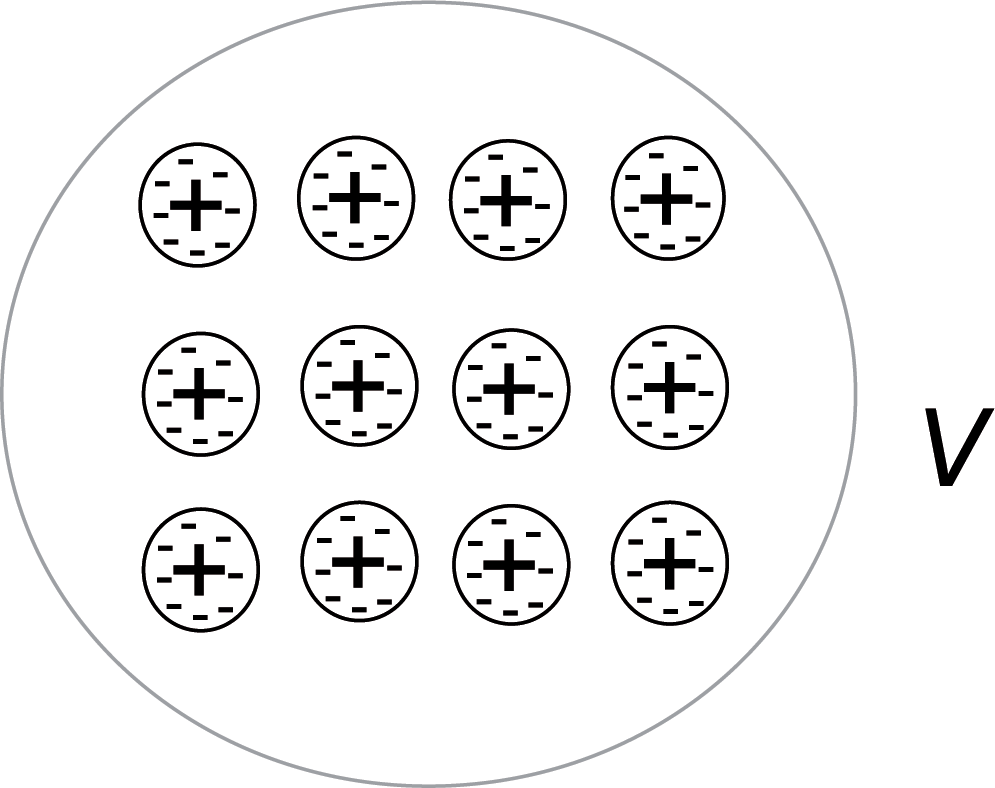
Figure 1: Apparently, the macroscopic (microscopically averaged) net charge at any location in a dielectric should always be zero.

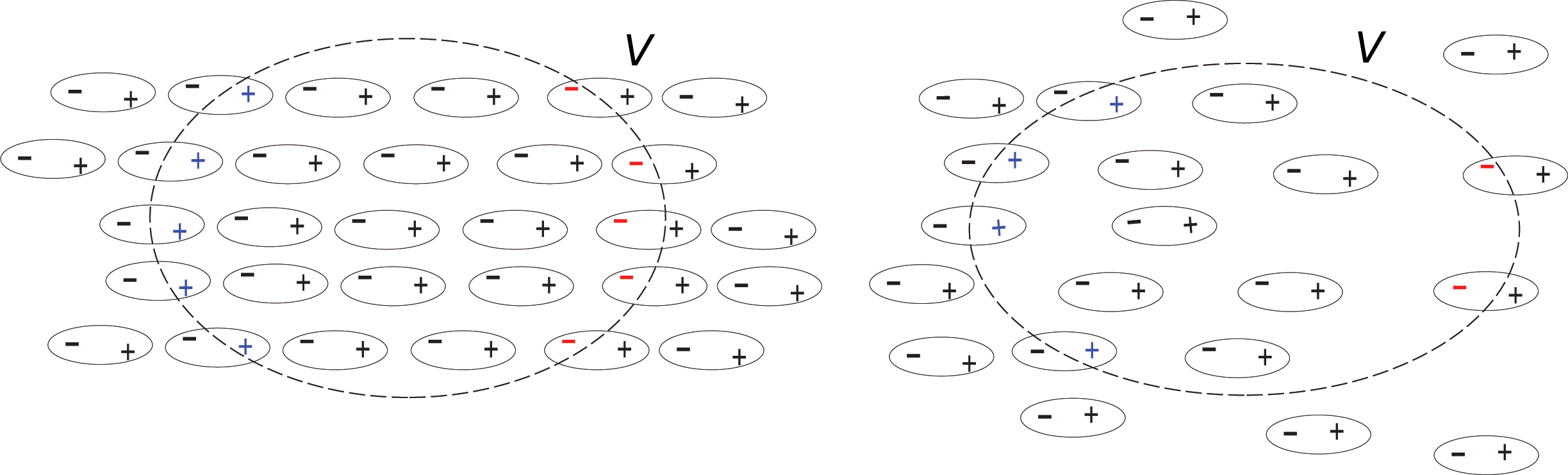
Figure 2: These rough schemes are only intended to illustrate how a “net macroscopic charge” can arise inside a dielectric. Left. Although the propagated electric field polarizes the molecules of the dielectric, if the dipolar moment distribution is spatially homogeneous — more accurately, if it does not diverge —, the net dielectric charge is zero at all “macroscopic” points.This is grafically motivated by assuming an horizontal (left-to-right) electric field and computing the net charge within a small “macroscopic” volume $V$ centered at some point. All dipoles within the volme contribute with zero net charge, while those “crossing” the left border (in this somewhat naive view) are also compensated by those crossing the right border. Right. When the dipolar moments are inhomogeneously distributed (namely, when $\nabla\cdot\mbox{\boldmath$\mathcal{P}$}=0$), nonzero dielectric charge arises. In this case, for example, the density of the material could be thought of as decreasing to the right, thus yielding a non-zero locally-averaged charge distribution.

The problem would be solved if the functional form of $\boldsymbol{p}$ with the applied field $\mathcal{E}$ were known. It appears reasonable to think that the dipole moments $\boldsymbol{p}$ somehow follow $\mathcal{E}$ since, if the electric force $\mbox{\boldmath$\mathcal{F}$}{}_{e}=-q\mbox{\boldmath$\mathcal{E}$}$) increases, the negative charge cloud will be displaced farther away from the (fixed) positive charge; this means that $\boldsymbol{s}$ will be increased, and so will $\boldsymbol{p}$ (and $\mathcal{P}$). Actually, for “moderate” field intensities, the relation between $\boldsymbol{p}$ and $\mathcal{E}$ can be taken as linear… but not necessarily instantaneous, as we will see next. Note, finally, that the result (10) is consistent with the qualitative reasoning illustrated in Fig. 2: only if the polarization vector diverges — which accounts for an inhomogeneous dipolar distribution —, can an effective dielectric charge exist.

The theoretical framework to calculate the form of $\mathcal{P}$ is the Quantum theory, but that is well beyond the scope of this lecture, so we will use the naive (yet fortunate) classical model of Lorentz, in which an electron responding to the electric field is envisioned as being bound to an atomic nucleus by an elastic force. The model is sketched in Fig. 3. We choose to call $x$ the polarization direction of the $\mbox{\boldmath$\mathcal{E}$};$ i.e., $\mbox{\boldmath$\mathcal{E}$}=\boldsymbol{\hat{x}}\mathcal{E}$. Then also, it can be accepted that $\boldsymbol{s}$ $=\boldsymbol{\hat{x}}s,$ as shown in the figure (this in indeed the case in isotropic dielectrics). Needless to say, the spring in Fig. 3 is fictitious and intended solely as a reminder that a force of elastic type binds the electron to the nucleus. Thus for a static electric field $\mbox{\boldmath$\mathcal{E}$}=-\hat{x}\mathcal{E}$ at the electron location, the Coulomb force must equal the elastic force, which, for small elongations, is proportional to the displacement of the electron from its equilibrium position:

$$ks=q\mathcal{E}\qquad\text{{{\small\{static electric field\}}}}\emph{.}$$ (12)

In the purely mechanical interpretation, (12) derives from Hooke’s law, which states that $F_{\text{elastic}}=ks$ for small elongations of the spring, with $k$ the elastic constant of the latter. Is is assumed here that the much more massive nucleus is hardly affected by the electric field and remains static at $x=0$. Relation (12) shows that $s\propto\mathcal{E},$ so that, according to (11), $P(\boldsymbol{r})\propto\mathcal{E}$ $(\boldsymbol{r}),$ as anticipated. But the electric field of a wave will always be time-varying, so the electron will experience accelerations, and the following dynamic equation must be applied rather than (12):

$$m\,\ddot{s}(t)=q\mathcal{E}(t)-k\,s(t)-\zeta\dot{s}(t).$$ (13)

The overdots denote time derivative, $d/dt.$ Relation (13) is the Abraham–Lorentz equation, and simply expresses Newton’s second law for the electron: its mass times its acceleration must equal the net force upon it. The forces involved are the Coulomb force (in the $+x$ direction), the elastic force (in the $-x$ direction), and a “dissipative” force, introduced ad hoc, which accounts for the unavoidable energy losses. In the mechanical model, it is attributed to the “friction” of the spring system, which opposes to the electron movement with a force proportional to its velocity $\dot{s}(t)$, $\zeta$ being the proportionality constant. In reality, losses are caused by different physical processes to be discussed in Subsection 2.4.

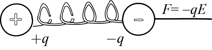
Figure 3: For small displacements around its equilibrium position ($s=0$), an active electron is bound to the nucleus by an elastic force ($F_{\text{elast}}=ks)$ symbolized by the spring. Isotropy is assumed in this model, i.e., $k$ is the same regardless of the spatial direction of $s.$

Only for a static situation, $d/dt=0$ and equation (13) obviously reduces to (12). Otherwise we see that the polarization does not follow the electric field instantaneously, because of the time derivatives. However, the differential equation (13) is linear with constant coefficients, so it describes a linear system which can be most easily understood in the frequency domain. Taking the Fourier transform (FT) of (13) (see Appendix), a linear, frequency-dependent relationship is obtained between the FTs of $\mathcal{E}(t)$ and $s(t),$ $E(\omega)$ and $S(\omega),$ respectively:

$$S(\omega)=\frac{q/m}{k/m-\omega^{2}+i\omega(\zeta/m)}E(\omega)\equiv K_{\text{diel}}(\omega)E(\omega).$$ (14)

If the input field is purely monochromatic, the phasor version (14) can be used — see Subsection A.2

The simplicity of (14) compared with (13) suggests that we carry on the derivations in the frequency domain if possible. Thus taking the FT of (11) and using (14), we obtain (omitting the variable $\boldsymbol{r}$ for clarity):

$$\boldsymbol{P}(\omega) =qN\boldsymbol{S}(\omega)=qNK_{\text{diel}}(\omega)\boldsymbol{E}(\omega)$$

$$\equiv\varepsilon_{0}\chi(\omega)\boldsymbol{E}(\omega)\qquad\text{{{\small\{linear and isotropic\}}}}\emph{.}$$ (15)

where $\chi(\omega)$ is the (linear) dielectric susceptibility, defined as the frequency-dependent polarization response of the dielectric to an electric field. For the moment, even if the appearance of $qNK_{\text{diel}}(\omega)$ arises from a fictitious model, we will keep to the equality $\chi(\omega)=qNK_{\text{diel}}(\omega)/\varepsilon_{0}$ implied in (15) as the functional form of the susceptibility. The unimportant prefactor $\varepsilon_{0}$ has been introduced for later convenience. Then,

$$\chi(\omega)=\dfrac{qN}{\varepsilon_{0}}\frac{q/m}{k/m-\omega^{2}+i\omega(\zeta/m)}\qquad\text{(Lorentz's model).}$$ (16)

A non-differential relationship can be established in the time domain between $\mathcal{P}$ and $\mathcal{E}$ through a convolution (Subsection A.3). Taking the FT^-1 of (15), we have

$$\mbox{\boldmath$\mathcal{P}$}(t)=\varepsilon_{0}\breve{\chi}(t)\ast\mbox{\boldmath$\mathcal{E}$}(t)=\varepsilon_{0}\int_{-\infty}^{\infty}\breve{\chi}(\tau)\mbox{\boldmath$\mathcal{E}$}(t-\tau)d\tau=\varepsilon_{0}\int_{0}^{\infty}\breve{\chi}(\tau)\mbox{\boldmath$\mathcal{E}$}(t-\tau)d\tau.$$ (17)

Thus $\breve{\chi}(t)=\,$FT${}^{-1}[\chi(\omega)]$ is the “impulse response” of the dielectric (at the particular point $\boldsymbol{r}$ considered), using the terminology of linear systems theory. The last equality in (17) follows from the causality of the response, that is, from the presumption that the polarization of the material at time $t$ cannot depend on the on the future electric field, at $\tau>t.$ This requirement can only be ensured in (17) if $\breve{\chi}(\tau)=0$ for $\tau<0$, a condition to which we indeed adhere. Then, the response of the dielectric at time $t$ depends on all the past history, $\tau\leq t,$ of the electric field. We then say that the dielectric response is dispersive in time.

$\mbox{\boldmath$\mathcal{J}$}{}_{d}(\boldsymbol{r},t),$ still unknown, is easily related to $\rho_{d}(\boldsymbol{r},t)$ through the law of conservation of charge: $\nabla\cdot\mbox{\boldmath$\mathcal{J}$}{}_{d}=-\partial\mbox{\boldmath$\mathcal{P}$}/\partial t.$ Using (10), it follows that

$$\mbox{\boldmath$\mathcal{J}$}_{d}(\boldsymbol{r},t)=\dfrac{\partial\,\rho_{d}(\boldsymbol{r},t)}{\partial\,t}.$$ (18)

Therefore, if the dielectric polarization varies with time, a dielectric current will be generated.

2.2 Wave equations in time and in frequency

Replacing (10) and (18) in (8), a time wave equation is obtained expressed in terms of the polarization (the variables $\boldsymbol{r},t$ are omitted):

$$\framebox{$\nabla^{2}\mbox{\boldmath$\mathcal{E}$}-\dfrac{1}{\varepsilon_{0}c^{2}}\dfrac{\partial^{2}}{\partial\,t^{2}}\left[\varepsilon_{0}\mbox{\boldmath$\mathcal{E}$}+\mbox{\boldmath$\mathcal{P}$}\right]=\left\{\begin{tabular}[]{l}$=-\dfrac{1}{\varepsilon_{0}}\nabla(\nabla\cdot\mbox{\boldmath$\mathcal{P}$})$\\ $=\text{ }0\text{\quad(or }\simeq 0\text{)}\quad\text{often}$\end{tabular}\ \right.\qquad\text{{{\small\{general\}}}}\quad$}$$ (19)

By general we mean that the equation also applies to nonlinear and/or anisotropic dielectrics, since the form of $\mathcal{P}$ is unspecified and not necessarily that of (17). Actually, (19) should be the starting point in the study of such cases, but here we will limit ourselves to (linear) isotropic, homogeneous dielectrics. While isotropy is already implicit in relation (15), homogeneity means $\boldsymbol{r}$-independence: $\chi(\boldsymbol{r},\omega)=\chi(\omega).$ Thus in this case the RHS of (19) is identically zero for linear response.

The term in square brackets on the LHS of (19) is defined as the electric displacement vector:

$$\mbox{\boldmath$\mathcal{E}$}(\boldsymbol{r},t)+\mbox{\boldmath$\mathcal{P}$}(\boldsymbol{r},t).$$ (20)

In order to obtain the homogeneous wave equation in a linear dielectric, we apply the FT to (19) and make use of (15), which leads to

$$\framebox{$\nabla^{2}\boldsymbol{E}+\dfrac{\omega^{2}}{c^{2}}n^{2}(\omega)\boldsymbol{E}=\mathbf{0}\qquad\left\{\begin{array}[]{l}\text{{{\small linear, isotropic}}}\\ \text{{{\small\& homogeneous}}}\end{array}\right\}$}$$ (21)

where

$$n(\omega)\equiv\sqrt{\varepsilon^{\prime}(\omega)}$$ (22)

is the (frequency-dependent) index of refraction, or refractive index, defined as the square root of the relative dielectric permittivity, which is in turn defined as

$$\varepsilon^{\prime}(\omega)\equiv 1+\chi(\omega).$$ (23)

Naturally, $\varepsilon^{\prime}$ and $n$ are $\boldsymbol{r}$-dependent if $\chi$ is. Note that, even if $\boldsymbol{E}=\boldsymbol{E}(\boldsymbol{r},\omega),$ no differential operator acts on $\omega,$ so the frequency is a parameter, rather than a variable, in the Fourier-transformed wave equation.

In the isotropic, linear (but not necessarily homogeneous) case, the FT of (20) yields

$$\boldsymbol{D}(\boldsymbol{r},\omega)=\varepsilon(\boldsymbol{r},\omega)\boldsymbol{E}(\boldsymbol{r},\omega)\qquad\text{{{\small\{linear and isotropic\}}}\emph{{\small,}}}$$ (24)

with $\varepsilon(\boldsymbol{r},\omega)\equiv\varepsilon_{0}\varepsilon^{\prime}(\boldsymbol{r},\omega),$ the (absolute) dielectric permittivity.

Eq. (21) displays the key effect of the dielectric almost blatantly. With $\varepsilon^{\prime}=1,$ (21) is obviously the wave equation in vacuum; this can also be checked by taking the FT of (9). Therefore, the wave equation in the dielectric is formally identical to that in vacuum, with the only difference that $c/n(\omega)$ appears in place of $c$. The index $n(\omega)$ is in general a complex quantity [see (22), (15) and (14)]. Calling the real and imaginary parts $n_{r}$ and $-n_{i},$ respectively (the minus sign is chosen for later convenience), we write

$$n(\omega)=n_{r}(\omega)-in_{i}(\omega).$$ (27)

If $n(\omega)$ were real, we could readily conclude, from the form of (21), that plane waves are again solutions of the wave equation in an homogeneous dielectric, only with their (frequency-dependent) velocity of propagation being $c/n(\omega)$ rather than $c.$ But since a complex velocity is meaningless, we will have to solve (21) explicitly.

Assuming a linearly-polarized ($\boldsymbol{E=\hat{u}}E$) plane wave propagating in the $z$ direction ($\nabla^{2}=\partial^{2}/\partial z^{2}$), a simple scalar wave equation is obtained:

$$\dfrac{d^{2}E(z,\omega)}{dz^{2}}+\dfrac{\omega^{2}}{c^{2}}n^{2}(\omega)E(z,\omega)=0.$$ (28)

2.3 Attenuated monochromatic waves

The general solution of (28) is

$$E(z,\omega)=A(\omega)e^{-i(\omega/c)n(\omega)z}+B(\omega)e^{i(\omega/c)n(\omega)z},$$ (29)

where $A(\omega)$ and $B(\omega)$ are the arbitrary integration constants (with respect to $z;$ remember $\omega$ is a mere parameter here). The first and second summands obviously correspond to forward and backward travelling waves along $z,$ respectively. We will assume forward propagation only and set $B(\omega)=0.$ Then $A(\omega)=E(0,\omega)$ is the FT of the electric field at $z=0.$ We now consider a purely monochromatic wave of discrete frequency $\omega_{0}.$ The corresponding phasor (Subsection A.2) is

$$\tilde{E}(z)=Ae^{-i(\omega_{0}/c)n(\omega_{0})z}=Ae^{-(\omega_{0}/c)n_{i}(\omega_{0})z}e^{-i(\omega_{0}/c)n_{r}(\omega_{0})z},$$ (30)

with $A\equiv A(\omega_{0}),$ which we assume real. The decomposition (27) has been employed in the second equality. The real temporal field is, thus,

$$\mathcal{E}(z,t)=\operatorname{Re}\left[\tilde{E}(z)e^{i\omega_{0}t}\right]=Ae^{-\,n_{i}(\omega_{0})(\omega_{0}/c)z}\cos\left(\omega_{0}t-n_{r}(\omega_{0})\frac{\omega_{0}}{c}z\right).$$ (31)

The argument of the cosine in (31) can be cast in the form $-n_{r}(\omega_{0})(\omega_{0}/c)[z-t\,c/n_{r}(\omega_{0})]$, which shows explicitly a functional dependence of the type $f(z-v_{\text{ph}}t)$, with

$$v_{\text{ph}}=v_{\text{ph}}(\omega_{0})=\frac{c}{n_{r}(\omega_{0})}.$$ (32)

Therefore, $v_{\text{ph}},$ called phase velocity, is the velocity of propagation of the phase of a sinusoidal (i.e., perfectly monochromatic) wave of frequency $\omega_{0}.$ This velocity does not describe the “velocity of the wave” as one would commonly understand it. This point will be clarified in Subsection 3.1.

We conclude that the phase velocity of a monochromatic wave in an homogeneous dielectric is $c$ divided by the real part of the refractive index. The imaginary part $-n_{i},$ which is always negative in normal, non-amplifying materials ($n_{i}>0$), ultimately arises from the imaginary-valued “friction” term $i\omega(\zeta/m)$ in (14), and accounts for the material losses. It results in the decreasing exponential factor in (31). The wave is thus progressively attenuated as it propagates, and $\mathcal{E}(z,t)$ has the damped form sketched in Fig. 4. In many practical cases, when the dielectric is almost transparent at the frequencies of interest, the approximations $n_{i}\simeq 0$ and $n\simeq n_{r}$ can be made, so that $v_{\text{ph}}\simeq c/n.$

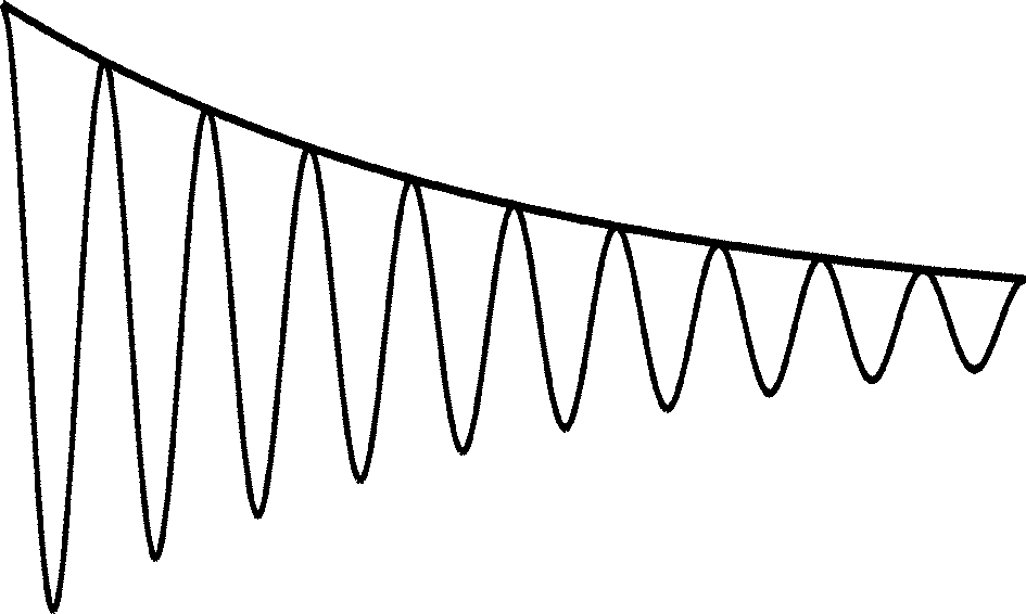
Figure 4: Form of the forward-propagating solution (31). (The exponential decay is greatly exagerated for illustration purposes.) Regardless of the spatial damping of the envelope, at each coordinate $z,$the wave is perfectly monochromatic.

The fact that the speed of light in a dielectric depends on its frequency is the key result of this section. This phenomenon of dispersive nature has abundant and important implications in Photonics.

2.4 The “true” frequency dependence of the refractive index

Lorentz’s classical model for the electron-field interaction displays two features which are qualitatively correct: the linear relationship between the polarization and the electric field (when the latter is not too large), and the dispersive nature of the dielectric response, which results in a frequency-dependent complex susceptibility $\chi(\omega)$. However, quantum-mechanical calculations show, to start with, that $\chi(\omega)$ is in reality made up of several (not only one) resonant contributions of the form (16), which thus appear in the actual forms of $\varepsilon^{\prime}(\omega)$ and $n(\omega)$ as well:

$$n(\omega)=\sqrt{\varepsilon^{\prime}(\omega)}=\sqrt{1+\chi(\omega)}=\sqrt{1+\sum\limits_{j=1}^{N}\frac{A_{j}\,\omega_{j}^{2}}{-\omega^{2}-i\omega\,b_{j}+\omega_{j}^{2}}},$$ (33)

or, in terms of the vacuum wavelength,

$$n_{\lambda}(\lambda)\equiv n(2\pi c/\lambda)=\sqrt{1+\sum\limits_{j=1}^{N}\dfrac{A_{j}\lambda^{2}}{\lambda^{2}-i\gamma_{j}\lambda-\lambda_{j}^{2}}},$$ (34)

with $\lambda_{j}=2\pi c/\omega_{j}$ and $\gamma_{j}=b_{j}\lambda_{j}^{2}/(2\pi c).$

The parameters $A_{j},$ $b_{j}$ and $\omega_{j}$ must be calculated through the quantum-mechanical formalism (or measured) for each material. One possible origin of the coefficients $b_{j}$ (responsible for the imaginary part of the refractive index) is the spontaneous emission. We briefly anticipate the quantum model of light-matter interaction, which essentially is viewed as the interplay of three processes. In the simplest picture, the monochromatic radiation of frequency $\nu=\omega/(2\pi)$ is comprised of a flux of photons with energy $E_{\text{p}}=h\nu$ each. If $E_{\text{p}}$ equals the energy difference between two atomic levels, some photons may be absorbed by atoms of the dielectric (absorption), which thus become temporarily excited. Thus, the photon disappears and its energy incorporates to the absorbing atom through the excitation of one of its electrons, which “jumps” from its original orbital to the higher-energy orbital; in the notation of (33), we have $\nu=$ $\omega_{j}/(2\pi),$ i.e., the radiation frequency has to coincide with one of the resonant frequencies. Next, the atom re-emits the photon, hopefully in the same direction and with the appropriate phase relationship — somehow “influenced” by the presence of the electromagnetic field (stimulated emission) — so as to keep contributing coherently to the global propagating field. The atom returns to its unexcited energy level, but the new photon can in turn be absorbed again by another atom of the material, which then will re-emit it, and so on. However, not all absorbed photons are re-emitted by stimulated emission; some excited atoms simply de-excite emitting a photon in a random direction and with unpredictable phase (spontaneous emission). Although such photons do not really disappear, they can be considered as “lost” for all propagation purposes. To be precise, some photons may be spontaneously emitted having, by chance, the right direction and the right phase to add coherently to the propagating field. However, statistically, the number of “lost” spontaneous photons is by far greater.

It should be noted that, although the photon “flies” across the interatomic vacuum at speed $c$, the accumulated processes of absorption-emission amount to modifying the phase of the resulting electromagnetic field so has to make $v_{f}=c/n_{r}(\omega).$ This modification of the phase velocity occurs at all frequencies, but it is particularly abrupt around the resonances, at which, in the quantum picture, actual absorptions and emissions of photons are much more likely to take place.

Note that, contrary to what one might at first think and is sometimes implied in the literature, the described absorption-emission cycles do not result in the slowing down of the pure monochromatic wave. A true monochromatic wave never starts or ends, so the absorption/emission events have been happening “forever” and it is meaningless to speak of “propagation delay”. Things will change in Section 3.

It can be seen in Fig. 5 that the real refractive index “wiggles” at any resonance frequency and can reach a value actually smaller than 1 on the right side. This is related to a phase shift (most easily described in classical terms, considering the interference between the incident wave and the wave radiated by the induced atomic dipoles), and of course is without consequences by itself.

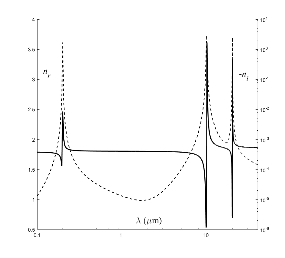
Figure 5: Real (solid line) and imaginary (dotted line) parts of the refractive index of an hypothetical dielectric material highly transparent in the near-IR, with resonances in the UV and mid-IR spectral ranges, as predicted by formula (33).

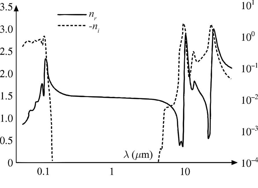
Figure 6: Actual shapes of the real and imaginary parts of the refractive index of the silica in the spectral range considered in the Fig. 5.

Concurring with the simple process of spontaneous emission described above, in real solids there are other mechanisms whereby photons may be effectively removed from the propagating field. Interaction with phonons is an important example. Phonons can be described as quanta of the (unavoidable) thermally-excited vibration modes of the molecules (these mechanical oscillations are energy-quantified in phonons, much like the electromagnetic field is in photons). Under certain circumstances, phonons can be excited at the expense of the energy of photons, which is thus lost as heat.

Fig. 5 illustrates the form of $n(\omega)$ according to (33) for an hypothetical material with three absorption peaks. However, by way of example, Fig. 6 shows the actual real and imaginary parts of the refractive index of the fused silica glass, which is an amorphous (or vitreous) form of silicon dioxide or silica, SiO${}_{2},$ the most important material in the current technology of optical fibers. Although there is some resemblance between the curves, the measured response of SiO₂ also shows remarkable differences with the simple behavior predicted by the Lorentz oscillators. It is obvious that a more complete, and presumably complicated, model of the material is required to describe its dielectric properties realistically. This is far beyond the scope of this presentation, so we will only make some qualitative considerations.

In solids, atoms are packed very close to each other, with the result that their outer orbitals overlap and interact strongly. As a result, the original discrete energy levels of the isolated atoms broaden and become (quasi) continuous bands. In fused silica, the electronic transitions (which we have attempted to describe by means of the Lorentz oscillators) involve tightly bound valence electrons of the SiO₂ molecules which excitation requires high energy photons corresponding to the ultraviolet (UV) spectral range. Other effects, such as interactions with excitons, make the modelling of the UV absorption even more complex. Thus, the continuous character of the spectral absorption in the UV region, makes it more difficult to model it by simple Lorentz’s oscillators.

Examining Fig. 6, we see that, moving to lower frequencies from the UV zone, there is a wide, almost transparent spectral range that reaches the near-infrared zone. As wavelength increases further within the infrared (IR) zone, the extinction coefficient grows rapidly again. The absorption in the IR, however, does not take place through interactions with electrons as in the UV, but through vibrational transitions. Think, for example, of a two-atom molecule of polar character (i.e., the spatial negative charge is located, say, closer to one of the atoms than the other, resulting in a permanent dipole moment). Thermal agitation may cause periodical stretching and shrinking of the interatomic distance, thus modulating the dipole moment. The situation resembles the modulation of the electronic dipoles depicted in Fig. 3. In the electronic interaction, however, the atoms or molecules were assumed to be nonpolar and it was the external optical field which produced the electronic dipoles by displacing the electronic charge from its equilibrium position. On the contrary, in the present case the dipole moments are pre-existing and their oscillations are thermally induced. As is inherent to the concept of phonon, the mechanical oscillations are collective (even in noncrystalline solids) and form wave patterns across the material. Therefore, the dipoles “riding” on these phonon waves can interact coherently with the IR electromagnetic waves. The phonons involved in these transitions are of the type called “TO” (transverse optical). As a first approximation, the displacement of the ions can be modelled by Lorentz oscillators, which yields an expression remarkably similar to (16) with the resonant frequency being the natural vibrational frequency of the TO phonon mode [5].

The model qualitatively described above only applies if the molecules of the glass have a non-zero dipole moment available to interact directly with the field. Silica is essentially non-polar, so the direct interaction with TO phonons is not possible. Nevertheless, other higher-order interactions involving several phonons can eventually give rise to the appearance of dipolar charge distributions with which the electric field can interact (multi-phonon absorption). In any event, even if some separated peaks are distinguishable in the IR region in Fig. 6, the actual features of the IR absorption cannot be accounted for by a simple Lorentz model.

In view of all the considerations made above, we may even wonder why bring up the Lorentz model at all. The good news is that, in the almost transparent spectral regions, formulas (33)–(34) work very satisfactorily for many materials. As far as optical fibers are concerned, transparency is indeed the desired situation, which in expression (34) occurs when $\lambda$ is between two resonances and sufficiently far from both (hence, from all others too), so that $|\lambda_{j}^{2}-\lambda^{2}|\,>>|\gamma_{j}\lambda|$ for all $\lambda_{j}.$ In this case the imaginary part of (34) is negligible and $n_{\lambda}(\lambda)$ becomes real:

$$n_{\lambda}(\lambda)=\left(1+\sum\limits_{j=1}^{N}\dfrac{A_{j}\,\lambda^{2}}{\lambda^{2}-\lambda_{j}^{2}}\right)^{1/2}\qquad$$Sellmeier’s formula  (35)

Many dielectric materials have their refractive index modelled by a Sellmeier expression with three terms in the sum. The parameters $A_{j}$ and $\lambda_{j},$ which are tabulated, are typically obtained by fitting the experimental data to the model.

2.5 Time and space frequencies, propagation constant, and wavelength

We will assume a dielectric with negligible losses hereafter and write $n$ for the real index The field (31) read:

$$\mathcal{E}(z,t)=A\cos\left(\omega t-n(\omega)\frac{\omega}{c}z\right)=A\cos\left(\omega t-k(\omega)z\right),$$ (36)

where we have replaced the symbol $\omega_{0}$ by $\omega$ to ease the notation (but remember that $\omega$ is not a variable: it is a fixed parameter!) In the last expression of (36) we have introduced the propagation constant or wavenumber vector, defined as

$$\framebox{$k(\omega)\equiv n(\omega)\dfrac{\omega}{c}\equiv n(\omega)k_{0},$}$$ (37)

where $k_{0}$ is, accordingly, the propagation constant in vacuum, in which $n(\omega)=1$ at all frequencies. Using (32), we see that

$$\framebox{$v_{\text{ph}}(\omega)=\dfrac{c}{n(\omega)}=\dfrac{\omega}{k(\omega)}.$}$$ (38)

If in (36) we fix the coordinate $z,$ we are left with a periodic time function, the period ($T$) being given by the condition $\omega(t+T)=\omega t+2\pi.$ This is,

$$T=\frac{2\pi}{\omega}.$$ (39)

If we fix time $t$ instead, we obtain a periodic spatial function, the spatial period ($\lambda$) being given by the condition $kz=k(z+\lambda)+2\pi,$ as sketched in Fig. 7. The spatial period is better known as wavelength. We thus obtain

$$\lambda=\frac{2\pi}{k}.$$ (40)

So we see that the propagation constant $k$ represents, in space, the “spatial frequency” expressed in radians/meter, just as $\omega$ represents, in time, the temporal frequency expressed in en radians/second. It also follows that $v_{\text{ph}}=\lambda/T=\lambda\nu,$ with $\omega=2\pi\nu.$

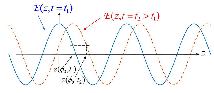
Figure 7: The propagation constant or wavenumber $k$ is the spatial angular frequency, just as $w$ is the time angular frequency. Its (spatial) period in the medium is $\lambda$, just as $T$ is the period in time. The figure shows a monochromatic wave across the spatial coordinate at two different frozen times

An important point to notice is that $\lambda$ is a function of $n$:

$$\lambda=\frac{2\pi}{k(\omega)}=\frac{1}{n(\omega)}\frac{2\pi c}{\omega}.$$ (41)

Consequently, since $c$ is a constant and the angular frequency $\omega$ is the same in all media, it follows from (41) that the wavelength is different in different media (according to $n$). When a laser is said to emit “at 1,55 $\mu$m,” it is understood that the given value is that in vacuum (or, to most practical effects, in air). In a different medium with an index $n,$ the wavelength would be different: $\lambda=\lambda_{0}/n,$ where $\lambda_{0}$ is the vacuum value. Fig. 8 illustrates this point.

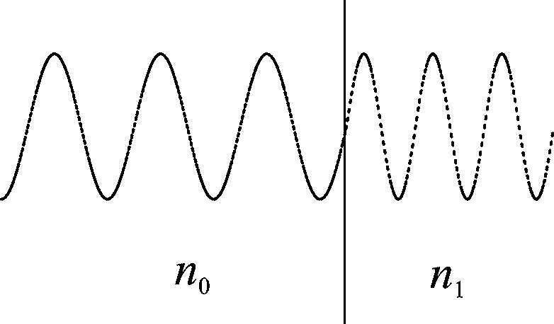
Figure 8: The propagation constant or wavenumber $k$ is the spatial angular frequency, just as $\omega$ is the time angular frequency. Its (spatial) period in the medium is $\lambda$, just as $T$ is the period in time. The figure shows a monochromatic wave across the spatial coordinate at two different frozen times.

3 Propagation of signals

The results obtained in Subsection 2.3 can only be a starting point in our discussion. Although a purely monochromatic wave (which, strictly speaking, does not exist) can be realized approximately by keeping a highly-coherent light source switched-on for a very long (“infinite”) time, it is utterly useless for the purpose of transmitting information. Think of a digital signal, for example. In order to transmit the sequence of ones and zeros, some kind of variation has to be added to the wave shape so as to single out the symbols. For example, an increased amplitude may mean the presence of a ”one”. Obviously, the envelope-modulated wave is no longer monochromatic. We are thus confronted with new situations that will require new concepts.

3.1 Group velocity

Suppose we modulate the amplitude of an optical monochromatic wave (the “carrier”), of angular frequency $\omega_{0},$ with a signal $g(t),$ as shown in Fig. 9. This modulated (plane) wave enters an homogeneous lossless dielectric of semi-infinite length, starting at the plane $z=0$. The initial electric field is thus $\mathcal{E}(z=0,t)=g(t)\cos(\omega_{0}t),$ and the wave propagates across the dielectric in the $+z$ direction. Inspired by (31), one might think that, at a distance $z=L,$ the propagated field would be: $\mathcal{E}(z=L,t)=g(t-L/v_{\text{ph}})\cos(\omega_{0}t-k(\omega_{0})L)=g(t-L/v_{\text{ph}})\cos[\omega_{0}(t-L/v_{\text{ph}})];$ this is, a mere time-delayed version of $\mathcal{E}(z=0,t)$, the delay being $L/v_{\text{ph}}.$ However, this is wrong. The concept of phase velocity is inherent to monochromatic waves, like (31), whereas $\mathcal{E}(z=0,t)$ is made up of the aggregation of different spectral contributions, as actually expressed by its FT.

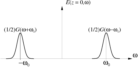
Figure 9: Optical spectrum. The bandwidth of the envelope-modulating pulse $g(t)$ is extremely small compared with the carrier frequency. It has been greatly exaggerated in the figure for visualization purposes.

At this point, the following argument is sometimes found in the literature: “Because the phase velocity $v_{\text{ph}}(\omega)=c/n(\omega)$ varies with frequency, ‘each frequency’ $\omega$ of the spectrum of the initial field $\mathcal{E}(z=0,t)$ will propagate at a different velocity $v_{\text{ph}}(\omega).$ Therefore, the different spectral components will not ‘arrive’ at the coordinate $z=L$ at the same time, and the pulse shape will be distorted (broadened).” This reasoning is very unfortunate for two reasons: (a) the concept of arrival time is meaningless for a spectral component, as discussed above; (b) the field envelope does indeed get distorted when $v_{\text{ph}}$ is frequency-dependent, but not because $v_{\text{ph}}$ is frequency-dependent; at least not with the naive (and erroneous) interpretation just expressed. We will go back to this point later, but we will first attempt to obtain the form $\mathcal{E}(z,t)$ under certain simplifying conditions.

We have been able to find a general solution of the wave equation in the frequency domain, (28), which we reproduce here assuming forward-propagation only ($B(\omega)=0$):

$$E(\omega,z)=A(\omega)e^{-i(\omega/c)n(\omega)z},$$ (42)

where $A(\omega)=E(z=0,\omega)$ is the spectral distribution or FT of the initial field $\mathcal{E}(z=0,t).$ Now,

$$\mathcal{E}(t,z=0)=g(t)\cos(\omega_{0}t),$$ (43)

with $g(t)$ the time-varying carrier envelope, which in our example of a digital signal has the shape of a pulse, but it could certainly be any arbitrary function of time representing an analog signal too. Taking the FT of (43), we obtain

$$E(\omega,z=0)=A(\omega)=\tfrac{1}{2}[G(\omega-\omega_{0})+G(\omega+\omega_{0})].$$ (44)

Using (43) in (42), we arrive at the expression of the FT of the propagated field at a distance $z$:

$$E(\omega,z)=\tfrac{1}{2}[G(\omega-\omega_{0})+G(\omega+\omega_{0})]e^{-i(\omega/c)n(\omega)z}.$$ (45)

Before calculating $\mathcal{E}(t,z),$ an important point must be noted. According to (45) and (44), the following relationship holds:

$$\dfrac{E(\omega,z)}{E(\omega,0)}=e^{-i\tfrac{\omega}{c}n(\omega)z}\equiv H_{d}(\omega).$$ (46)

So, the dielectric medium of length $z$ can be considered as a linear system characterized by a transfer function $H_{d}(\omega)$ relating the output and input fields. Since we have assumed that $n(\omega)$ is real, $|H_{d}(\omega)|=1;$ hence the dielectric is an all-pass filter, with flat amplitude response. To be precise, even admitting a small attenuation, the losses in optical fibres are essentially frequency-independent within the spectral width of the transmitted signals. Thus $H_{d}(\omega)=K\exp\left(-i\,(\omega/c)\,n_{r}(\omega)z\right)$ with $K<1$ but constant, so the transfer function is still flat in modulus. Then, any signal distortion will be entirely due the to phase of the dielectric response of the dielectric, as we will soon see.

There only remains to obtain $\mathcal{E}(t,z)$ by simply taking the FT^-1 of (45):

$$\mathcal{E}(t,z) =\frac{1}{2\pi}\int\nolimits_{-\infty}^{\infty}E(\omega,z)\,e^{i\omega t}d\omega$$

$$=\frac{1}{2\pi}\int\nolimits_{-\infty}^{\infty}\tfrac{1}{2}[G(\omega-\omega_{0})+G(\omega+\omega_{0})]\,e^{i\,[\omega\,t-k(\omega)\,z]}d\omega.$$ (47)

In (47) we have introduced the propagation constant (37). The physical interpretation of expression (47) is almost straightforward, but contains a subtle point. The propagated field is described as the sum of infinite quasi-monochromatic differential contributions $d\mathcal{E}(t,z)$ of spectral width $d\omega$, each located around a frequency $\omega$. A phase velocity $v_{\text{ph}}(\omega)$ seems naturally associated to the contribution $d\mathcal{E}(z,t)$ centered at $\omega$, so one might think that each of such partial fields propagates at the velocity $v_{\text{ph}}(\omega).$ This is mathematically wrong, as we see below.

In principle, in order to integrate (47) we need to know $G(\omega)$ — hence the pulse shape $g(t)$ — and, of course, the specific form of $n(\omega).$ Besides, the integration would have to be performed (most likely, numerically) for each and every $g(t)$ and $n(\omega)$ we were to consider. Fortunately, we can do better than that to some extent. Note that the optical carrier frequency $\nu_{0}=(2\pi)^{-1}\omega_{0}$, corresponding to a vacuum wavelength $\lambda_{0}\approx 1$ $\mu$m, will always be in the range $\nu_{0}\gtrsim 10^{14}$ Hz in our applications. On the contrary, the bandwidth $\Delta f$ of the transmitted signals — in this example, $g(t)$ — can typically be up to some $10$ – $20$ GHz (a bit rate of 10 Gb/s is standard). Then $\Delta f<<\nu_{0}$ always, and the spectrum of the optical field has indeed the form sketched in Fig. 9, which has the features a very narrow band-pass signal. In other words, $G(\omega-\omega_{0})$ is virtually zero as soon as $\omega$ moves a little bit away (relatively) from $\omega_{0}.$ The same applies to $G(\omega+\omega_{0})$ with respect to $-\omega_{0}.$ Consequently, we will assume as a start that we can approximate $n(\omega)$ around $\omega_{0}$ through a Taylor series with few terms, perhaps two or three, in the summand of $G(\omega-\omega_{0})$ in (45). Such approximation breaks down when $\omega$ is away from $\omega_{0}$, but we do not care since the distant frequencies do not contribute to the integral anyway, as $G(\omega-\omega_{0})\simeq 0$ there. An analogous approximation applies to $-\omega_{0}.$

Writing $\omega=\omega_{0}+\Omega,$ we have, for $\omega$ near $\omega_{0},$

$$n(\omega)=n(\omega_{0}+\Omega)=n_{0}+n_{1}\Omega+\tfrac{1}{2}n_{2}\Omega^{2}+\tfrac{1}{6}n_{3}\Omega^{3}+\cdots,$$ (48)

with $n_{0}=n(\omega_{0})$ and $n_{j}=d^{(j)}n(\omega)/d\omega^{j}|_{\omega_{0}}.$ We can also expand $k(\omega)$ directly:

$$k(\omega)=k(\omega_{0}+\Omega)=k_{0}+k_{1}\Omega+\tfrac{1}{2}k_{2}\Omega^{2}+\tfrac{1}{6}k_{3}\Omega^{3}+\cdots,$$ (49)

with $k_{0}=k(\omega_{0})$ and $k_{j}=d^{j}k(\omega)/d\omega^{j}|_{\omega_{0}}.$ The relationship between the coefficients $k_{j}$ and $n_{j}$ is straightforward:

$$k(\omega_{0}+\Omega)=n(\omega_{0}+\Omega)\frac{\omega_{0}+\Omega}{c}=\underset{k_{0}}{\underbrace{\frac{\omega_{0}}{c}n_{0}}}+\underset{k_{1}}{\underbrace{\frac{1}{c}(n_{0}+n_{1}\omega_{0})}}\Omega+\underset{(1/2)k_{2}}{\underbrace{\frac{1}{c}\left(n_{1}+\tfrac{1}{2}\omega_{0}n_{2}\right)}}\Omega^{2}+\cdots$$ (50)

For the moment we will assume that $n(\omega)$ can be approximated around $\omega_{0}$ with only two terms, i.e., $n_{2}=n_{3}=\cdots\simeq 0.$ Also, since $\Omega<<\omega_{0},$ we will neglect $\tfrac{1}{c}n_{1}\Omega^{2}$ as compared with $\frac{1}{c}n_{1}\omega_{0}\Omega.$ Then only $k_{0}$ and $k_{1}$ need be retained in (49). Moreover, the unquestionable band-pass character of $\mathcal{E}(z,t)$ allows us to make use of all associated approximations, as explained in Subsection A.4. We can thus operate only with the positive frequency spectrum, $G(\omega-\omega_{0}).$ Denoting $\mathcal{\tilde{E}}(z,t)$ the analytical field, and setting $k(\omega)=k(\omega_{0}+\Omega)\simeq$ $k_{0}+k_{1}\Omega,$ (47) yields

$$\mathcal{\tilde{E}}(z,t) \simeq\frac{1}{2\pi}\int\nolimits_{-\infty}^{\infty}G(\Omega)\,e^{i[(\omega_{0}+\Omega)t-(k_{0}+k_{1}\Omega)z]\,}d\Omega$$

$$=e^{i(\,\omega_{0}t-k_{0}z)\,}\frac{1}{2\pi}\int\nolimits_{-\infty}^{\infty}G(\Omega)\,e^{i[\Omega\,(t-k_{1}z)]\,}d\Omega=e^{i(\,\omega_{0}t-k_{0}z)\,}g(t-k_{1}z),$$ (51)

where the property (129) has been used in the last equality. Thus, we finally obtain

$$\mathcal{E}(z,t)=\operatorname{Re}[\mathcal{\tilde{E}}(z,t)]=g(t-z/k_{1}^{-1})\cos(\omega_{0}t-k_{0}z).$$ (52)

Expression (52) shows that the monochromatic carrier propagates at its corresponding phase velocity $v_{\text{ph}}(\omega_{0})=c/n_{0}=\omega_{0}/k_{0},$ but the envelope — which contains the transmitted information — propagates at a different velocity, given by $k_{1}^{-1}=(dk/d\omega)_{\omega=\omega_{0}}^{-1}=(d\omega/dk)_{\omega=\omega_{0}}.$ We will call this the group velocity (“at $\omega_{0}$”):

$$\framebox{$v_{g}(\omega_{0})=\left.\dfrac{d\omega}{dk}\right|_{\omega=\omega_{0}}.$}$$ (53)

Compare (53) with the phase velocity of the carrier, (38), which we re-write here:

$$\framebox{$v_{p}(\omega_{0})=\dfrac{\omega_{0}}{k_{0}}.$}$$ (54)

Fig. 10 illustrates the difference between both velocities geometrically.

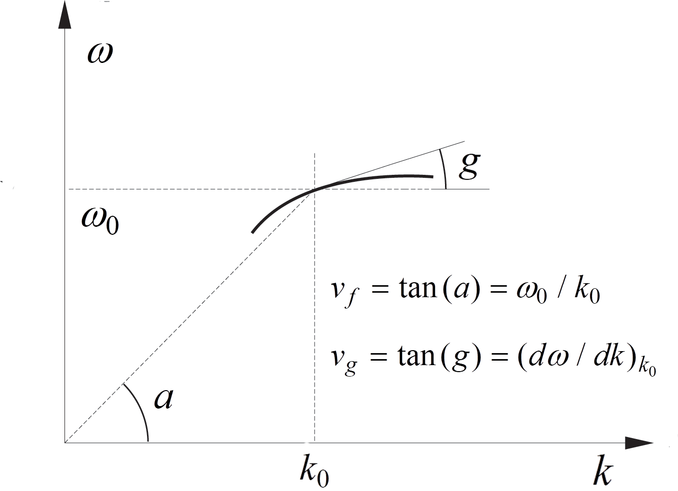
Figure 10: Geometrical interpretation of the phase and group velocities.

The result (52) does not display any distortion of the wave shape, but just a pure propagation delay of value $z/v_{g}.$ This is mathematically understandable because, in truncating the expansion of $k(\omega)$ to just two terms, the only effect of $k(\omega)$ is the time shift induced by the linear summand $i\Omega k_{1}z$ in the exponent of the Fourier integral. We have then arrived at an important conclusion: Distortionless propagation requires that the propagation constant have a linear dependence with frequency, $k(\omega)=k(\omega_{0})+k_{1}(\omega-\omega_{0})$ (at least, within the spectral range of the signal). Now, when is $k$ exactly (not approximately) linear with $\omega$? Equation (50) gives the answer: only when $n(\omega)$ is strictly constant; if $n(\omega)$ does not vary with $\omega$ around $\omega_{0}$ ($n_{1}=n_{2}=n_{3}=\cdots=0$), all $k_{j}$ with $j>1$ are exactly zero and $k$ is linear. Moreover, in this case the phase and group velocity coincide, since $v_{g}^{-1}=k_{1}=n_{0}/c$. Note that the linear dependence that we assumed to obtain (52) was an approximation in the first place, as we neglected the contribution of $n_{1}\neq 0$ to the coefficient of $\Omega^{2}.$

In a situation with a truly constant $n,$ the phase velocity is the same at all frequencies (as in vacuum), which means that no spectral component experiences any phase modification different from all other components; as a result, there is no distortion. Unfortunately, Sellmeier’s formula (35) warns us that the idea of a constant refractive index $n$ in some spectral range is unreal, and even a still more convincing argument will be outlined in Subsection 3.5. Thus, one or more higher-order terms must usually be considered, according to the degree of accuracy sought. As we will soon see, these terms unavoidably bring about distortion.

If, however, the distortion is moderate (or, at least, no so dramatic that the pulse becomes unrecognizable), there is no reason to discard the concept of group velocity to describe the velocity at which the envelope (whether being distorted or not) moves. Even more, it will be useful to define a “group refractive index” such that, analogous to the relationship $v_{\text{ph}}=c/n,$ we can write

$$v_{g}(\omega)=\dfrac{c}{n_{g}(\omega)}\qquad$$definition of group index (55)

Using (55), (53) and (37), the relationship between both indices is obtained:

$$\framebox{$n_{g}(\omega)=n(\omega)+\omega\dfrac{dn(\omega)}{d\omega}.$}$$ (56)

Formula (56) is consistent with the fact that, if (hypothetically) $n(\omega)$ is constant, then $n_{g}=n$ and $v_{\text{ph}}=v_{g},$ as mentioned above. Other than in this ideal case, Fig. 5 shows that, in the lossless frequency ranges between resonances, the (virtually real) index $n(\omega)$ is always an increasing function of $\omega$. Then, $dn/d\omega>0$ and $n_{g}(\omega)>n_{\text{ph}}(\omega),$ implying that $v_{g}(\omega)<v_{\text{ph}}(\omega).$ Expression (56) can be written in terms of $\lambda$ through the definition(34):

$$\framebox{$n_{g\lambda}(\lambda)=n_{\lambda}(\lambda)-\lambda\dfrac{dn_{\lambda}(\lambda)}{d\lambda},$}$$ (57)

with $n_{g\lambda}(\lambda)\equiv n_{g}\left(2\pi c/\lambda\right).$

Obviously, the time it takes the pulse envelope to travel a specified distance ($L$), when the wavelength of the optical carrier is $\omega_{0},$ denoted $\tau_{g}(\omega_{0})$ [$=\tau_{g}(2\pi c/\lambda_{0})\equiv\tau_{g\lambda}(\lambda_{0})$] and formally called group delay, is given by

$$\tau_{g}(\omega_{0})=\dfrac{L}{v_{g}(\omega_{0})}\qquad\text{{\small definition\ of\ group\ delay.}}$$ (58)

The meaning of the group velocity under “unusual” circumstances (for example, near the resonances) is briefly discussed in Subsection 3.6.

3.2 Dispersion and envelope distortion

A true frequency-independent refractive index is physically unreal. A non-dispersive index can only be taken, at most, as a first approximation which accuracy will suffice or not depending on the specific problem at hand. We will first consider that, at least, one additional summand is required in the Taylor expansion of $k(\omega);$ this is, we will the keep the $\tfrac{1}{2}k_{2}\Omega^{2}$ term in (49). In general, the presence of this new quadratic term in the exponent of (51) yields the integral analytically unsolvable. Therefore, numerical integration would be required for each specific form of $g(t).$ Fortunately, we can still obtain some estimative, general results which will provide us with insight into the effects of the dispersion. Even if we cannot calculate the shape of the propagated pulse without actually solving the Fourier integral, we anticipate that the pulse envelope will most likely broaden, and we will attempt to estimate such broadening.

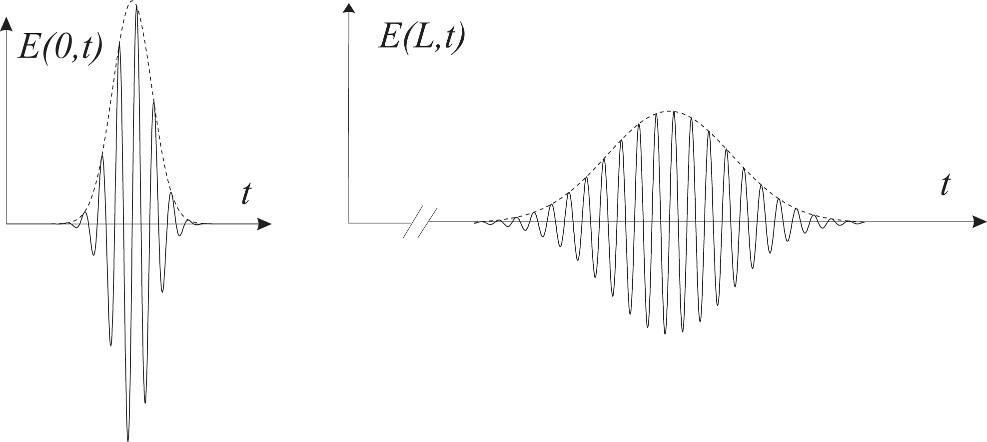
Figure 11: Sketch of the expected pulse broadening.

The left part of Fig. (11) shows the form of the spectrum of the optical signal at $z=0.$ As mentioned, we only need to consider the positive frequencies. Assume that the frequency dependence of the group velocity around $\omega_{0}$ is as sketched in Fig. 12 in solid line. The result that the envelope propagates, as a whole, at a velocity $v_{g}(\omega_{0})$ was obtained within the approximation $k(\omega_{0}+\Omega)\simeq k_{0}+k_{1}\Omega.$ To obtain some information about the distortion of the pulse shape, we need to be more subtle. Let us pick two narrow slices from the spectrum, as shown in Fig. 12. We will call them “sub-spectra” $R$ and $L$, respectively; they also include the corresponding negative-frequency parts, not shown in the figure. Their separation is chosen so that it roughly corresponds to the relevant spectral width of $G(\Omega).$To the narrow sub-spectra $R$, if considered isolated from the rest of the spectrum, there corresponds a “sub-pulse” envelope $g_{R}(t)$ in the time domain. Owing to a basic property of the Fourier-transformed pairs, $g_{R}(t)$ is expected to be less abrupt and longer in duration than the whole pulse envelope $g(t)$. Similarly, another sub-pulse $g_{L}(t)$ will correspond to the sub-spectra $L$. But, in view that the energy corresponding to $g_{R}(t)$ is closely located around $\omega_{0}+\Delta\omega/2,$ we see that the group velocity at which $g_{R}(t)$ propagates will be given more accurately by $v_{R}=v_{g}(\omega_{0}+\Delta\omega/2),$ rather than $v_{g}(\omega_{0}).$ Likewise, $g_{L}(t)$ will propagate at the velocity $v_{L}=v_{g}(\omega_{0}-\Delta\omega/2).$ Formally stated, we expand $\beta(\omega)$ to first order again, but this time around $\omega=\omega_{0}-\Delta\omega/2$ for $g_{L}(t),$ and around $\omega=\omega_{0}-\Delta\omega/2$ for $g_{R}(t)$, and we can write both “partial” optical fields as

$$\mathcal{E}_{\text{sub 1}}(t,z) =g_{L}(t-z/v_{L})\cos(\omega_{0}t-\beta_{L}z)$$ (59)

$$\text{ }\mathcal{E}_{\text{sub 2}}(t,z) =g_{R}(t-z/v_{R})\cos(\omega_{0}t-\beta_{R}z).$$ (60)

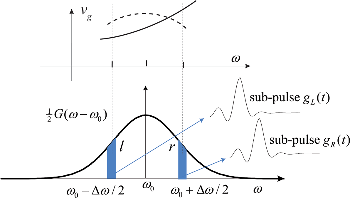
Figure 12: Rough estimation of the pulse broadening by considering the spectral dependence of $v_{g}(\omega).$ See text.

According to the graphic of $v_{g}(\omega)$ in Fig. 12, $g_{R}(t)$ propagates faster than $g_{L}(t);$ therefore, the resulting total pulse envelope will necessarily broaden, as sketched in Fig. 11. We will assume that the broadening of the whole original pulse $g(t)$ after propagation can be reasonably estimated as the accumulated temporal delay between the two isolated sub-pulses. Consequently, we focus on these subpulses and their associated spectral “slices”. Then, in travelling from $z=0$ to $z=L,$ the envelope $g(t)$ will broaden by an amount $\Delta\tau,$ given by

$$\Delta\tau\simeq\left|\dfrac{L}{v_{R}}-\dfrac{L}{v_{L}}\right|=L\left|v_{g}^{-1}(\omega_{0}+\Delta\omega/2)-v_{g}^{-1}(\omega_{0}-\Delta\omega/2)\right|.$$ (61)

But

$$v_{g}^{-1}(\omega_{0}+\Delta\omega/2) \simeq v_{g}^{-1}(\omega_{0})+\left(\dfrac{\Delta\omega}{2}\right)\left.\dfrac{dv_{g}^{-1}}{d\omega}\right|_{\omega_{0}}+\frac{1}{2}\left(\dfrac{\Delta\omega}{2}\right)^{2}\left.\dfrac{d^{2}v_{g}^{-1}}{d\omega^{2}}\right|_{\omega_{0}}$$

$$=v_{g}^{-1}(\omega_{0})+\left(\dfrac{\Delta\omega}{2}\right)\frac{1}{2}k_{2}+\left(\dfrac{\Delta\omega}{2}\right)^{2}k_{3}$$ (62)

$$v_{g}^{-1}(\omega_{0}-\Delta\omega/2) \simeq v_{g}^{-1}(\omega_{0})-\left(\dfrac{\Delta\omega}{2}\right)\frac{1}{2}k_{2}+\left(\dfrac{\Delta\omega}{2}\right)^{2}k_{3},$$ (63)

where (53) has been used, and $k_{2}$ and $k_{3}$ are defined in (49), and now named as follows:

$$k_{2} \equiv\,\left.\frac{d^{2}k}{d\omega^{2}}\right|_{\omega_{0}}\qquad\text{{\small Dispersion Parameter or GVD, \textquotedblleft Group Velocity Dispersion\textquotedblright} }$$ (64)

$$k_{3} \equiv\,\left.\frac{d^{3}k}{d\omega^{3}}\right|_{\omega_{0}}\qquad\text{{\small Dispersion Parameter of 2nd order.}}$$ (65)

Then, replacing (62) and (63) in (61), we obtain

$$\framebox{$\Delta\tau=k_{2}L\Delta\omega\qquad\text{{{\small\{1st-order dispersion only\}}}}$}$$ (66)

Quite reasonably, the pulse broadening turns out to be proportional to the propagation distance and increases with the spectral width of the propagated signal. The coefficient $k_{2}$ obviously depends on the dielectric material through $n(\omega).$ Note that if $k_{2}=0$ no pulse broadening is predicted, but only because the higher-order coefficients have not been taken into account.

Suppose now that $v_{g}(\omega)$ is not a monotonously increasing (or decreasing) function around $\omega_{0},$ but has an extreme (maximum or minimum) precisely at $\omega_{0},$ as shown in Fig. 12 in dashed line. Then $k_{2}=0,$ but the dispersion does not disappear as $v_{g}$ still varies with $\omega.$ As noted above, this should be accounted for by $k_{3}.$ However, for symmetry reasons, the terms with $k_{3}$ happen to cancel out when subtracting (62) and (63), so we need to change the locations of the sub-spectra to allow for $k_{3}$ to manifest itself. We will compute the delay between a sub-pulse corresponding to $\omega_{0}$ [which is $L/v_{g}(\omega_{0}$ ] and that of the sub-pulse at $\omega_{R}=\omega_{0}+\Delta\omega/2$ (choosing $\omega_{L}$ instead is indistinct).

From (62) with $k_{2}=0,$ we obtain

$$|v_{g}^{-1}(\omega_{0}+\Delta\omega/2)-v_{g}^{-1}(\omega_{0})|=\frac{1}{8}\left(\Delta\omega\right)^{2}k_{3}\,,$$ (67)

Thus,

$$\framebox{$\Delta\tau=\frac{1}{8}k_{3}L(\Delta\omega)^{2}\qquad\text{{{\small\{2nd-order dispersion only\}}}}$}$$ (68)

Results (66) and (68) display the linear dependence of $\Delta\tau$ with the propagation distance $L.$ Naturally, the frequency-dependent nature of the refractive index, often referred to as chromatic dispersion, is the ultimate cause of these distortive effects.

Expression (68) also shows that, when 2nd order dispersion dominates, the pulse broadening is proportional to the signal bandwidth squared. The wavelength $\lambda_{\text{ZD}}$ at which $k_{2}(\omega)$ is zero ($k_{2}(2\pi c/\lambda_{\text{ZD}})=0$) is usually called “zero-dispersion wavelength,” but it must be understood that it refers to the 1st-order dispersion only; in general, the dispersion will be minimum, but not zero, at $\lambda=\lambda_{\text{ZD}}.$

3.3 Dispersion and residual frequency modulation or “chirp”

In addition to the distortion of the time envelope of the pulse, which we have roughly estimated above, the 1st-order dispersion ($k_{2}$) necessarily gives rise to another effect: the frequency modulation (FM) of the optical carrier. It is easy to understand why. Working with the analytical part of (47) and expanding $k(\omega_{0}+\Omega)$ to 2nd order in $\Omega$ around $\omega_{0},$ we have, in the customary narrow-band situation,

$$\tilde{\mathcal{E}}(z,t) =\frac{1}{2\pi}\int\nolimits_{-\infty}^{\infty}G(\Omega)\,e^{i\,[(\omega_{0}+\Omega)\,t-k(\omega_{0}+\Omega\,)\,z]}d\Omega$$

$$\simeq e^{i\,(\omega_{0}\,t-k_{0}\,z)}\frac{1}{2\pi}\int\nolimits_{-\infty}^{\infty}G(\Omega)\,e^{i\,\Omega(t-z/v_{g})}e^{-i\frac{1}{2}\,k_{2}\Omega^{2}z}d\Omega.$$

$$\equiv e^{i\,(\omega_{0}\,t-\beta_{0}\,z)}\tilde{g}(t,z)\equiv e^{i\,(\omega_{0}\,t-\beta_{0}\,z)}|\tilde{g}(t,z)|e^{i\gamma(t,z)},$$ (69)

with $\tilde{g}(t,z)=\,$FT${}^{-1}[G(\Omega)\exp(-i\tfrac{1}{2}\,k_{2}\Omega^{2}z)].$ Note that $\tilde{g}(t,z)$ is a “baseband” signal as its spectrum contains no optical frequencies. The real field is

$$\mathcal{E}(z,t)=\operatorname{Re}[\tilde{\mathcal{E}}(z,t)]=|\tilde{g}(t,z)|\cos[\omega_{0}\,t-\beta_{0}\,z+\gamma(t,z)].$$ (70)

with

$$\tilde{g}(t,z)=|\tilde{g}(t,z)|e^{i\gamma(t,z)}.$$ (71)

Now the instantaneous frequency is defined as the time derivative of the phase (divided by $2\pi$):

$$\nu_{\text{ins}}(t)=\frac{1}{2\pi}\frac{d}{dt}[\omega_{0}\,t-\beta_{0}\,z+\gamma(t,z)]=\nu_{0}+\frac{1}{2\pi}\frac{d\gamma(t,z)}{dt},$$ (72)

with $\nu_{0}=\omega_{0}/(2\pi).$ Thus in general, only if $\gamma(t,z)=0$ there will be no frequency modulation. In view of (71), this condition is equivalent to $\tilde{g}(t,z)$ being a real valued-function. However, $\tilde{g}(t,z)$ is generally not real, a fact that can be readily verified by checking that $\tilde{g}(t,z)\neq\tilde{g}^{\ast}(t,z)$:

$$\tilde{g}^{\ast}(t,z) =\left[\frac{1}{2\pi}\int\nolimits_{-\infty}^{\infty}G(\Omega)\,e^{i\,\Omega(t-z/v_{g})}e^{-i\frac{1}{2}\,k_{2}\Omega^{2}z}d\Omega\right]^{\ast}$$

$$=\frac{1}{2\pi}\int\nolimits_{-\infty}^{\infty}G(\Omega)\,e^{i\,\Omega(t-z/v_{g})}e^{i\frac{1}{2}\,k_{2}\Omega^{2}z}d\Omega\neq\tilde{g}(t,z),$$ (73)

unless $k_{2}=0.$ Consequently, except in the non-dispersive case, there will be an instantaneous variation of the frequency around its “nominal” value $\omega_{0},$ which will depend on $k_{2}$ and the pulse shape at each $z$. This residual frequency modulation is called chirp. Fig. 13 illustrates this concept.

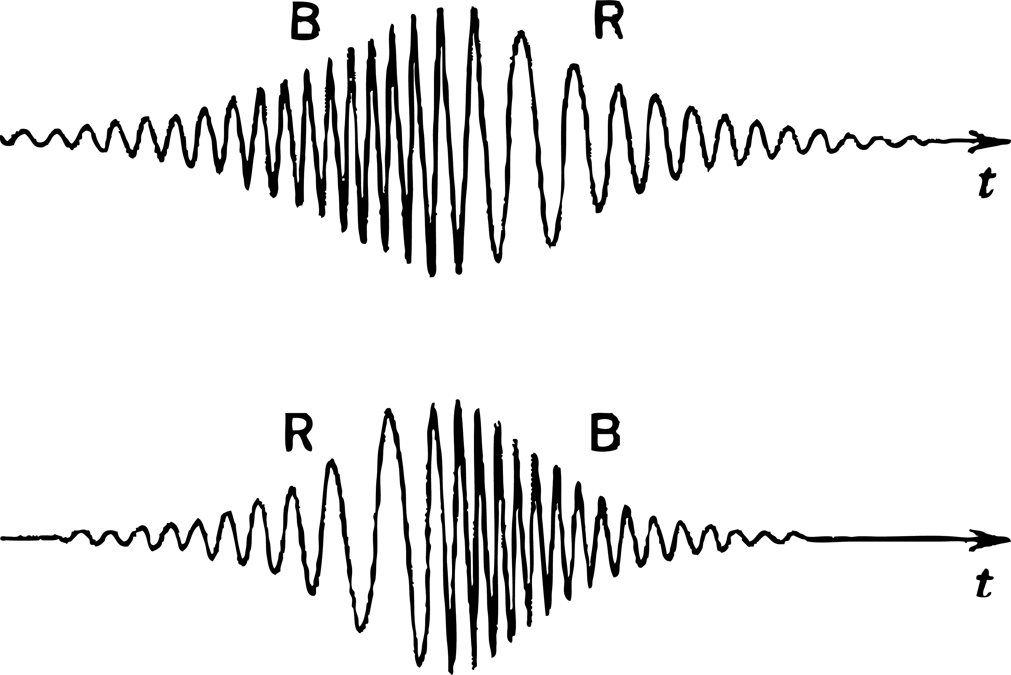
Figure 13: Example of a chirped pulse. Linear chirp has been assumed: $\nu(t)=\nu_{0}+at$, with $a$ being a real constant. Above: $a<0$ In this case, $\nu(t)$ is higher at the beginning of the pulse, which thus contains the (instantaneous) “blue” frequencies, while the tail contains the “red”, lower frequencies. Below: $a>0,$ which results in the opposite situation. For the sake of visualization, the frequency modulation has been greatly exaggerated.

Note that if there were only 2nd-order dispersion, a factor $\exp(-i\frac{1}{6}k_{3}\Omega^{3}z),$ odd in $\Omega,$ would replace $\exp(-i\frac{1}{2}k_{2}\Omega^{2}z)$ in the first integral of (73), with the final result that $\tilde{g}(t,z)=\tilde{g}^{\ast}(t,z).$ Therefore, 2nd-order dispersion alone would cause no chirp.

3.4 Dispersion in terms of the wavelength

Relations (66) and (68) are frequently written in an equivalent form, but with all parameters expressed in terms of the wavelength rather than the frequency. With this purpose, we define a parameter called simply “dispersion” and denoted by $D$, which, as we will see, plays the same role as $k_{2}$. By definition,

$$D(\lambda)\equiv\frac{1}{L}\frac{d\tau_{g}(\lambda)}{d\lambda}\qquad\text{{\small Definition of dispersion.}}$$ (74)

Consequently, $D(\lambda)$ expresses how the propagation time varies with the wavelength because of the group velocity dispersion, which is the ultimate origin of the time envelope distortion. Namely, we see that $D(\lambda)$ represents the temporal broadening of the propagated pulse envelope per unit propagation length, per unit wavelength width of the spectrum, when the latter is located around $\lambda$ (the optical carrier). The common units of $D$ are ps/(km$\times$nm). Now, using (58) and (53) in (74), it follows that

$$D=-\frac{2\pi\,c}{\lambda^{2}}k_{2},$$ (75)

and, using (75) and [$\Delta\omega=-(2\pi c/\lambda^{2})\Delta\lambda$], expression (66) can be written in the following alternative form:

$$\framebox{$\Delta\tau=DL\Delta\lambda\qquad\text{{{\small\{1st-order dispersion only\}}}}$}$$ (76)

In (76) and (66), it is understood that only the absolute value of $\Delta\tau$ matters. For example, $D<0$ ($k_{2}>0$) simply means that $v_{g}$ increases with $\lambda$ (because $n_{g}$ decreases with $\lambda$) — a situation labelled as normal dispersion. In this case, the sign of $\Delta\tau$ comes out negative in (76), which only means that the subpulse $g_{R}(t)$ arrives before than $g_{L}(t)$. When $D>0$ ($k_{2}<0$), $n_{g}$ increases with $\lambda$ ($v_{g}$ decreases with $\lambda$), which is called anomalous dispersion.

The alternative for $k_{3}$ is the dispersion slope or differential dispersion, $S,$ defined as:

$$S\equiv\frac{dD}{d\lambda}=\frac{4\pi\,c}{\lambda^{3}}k_{2}+\left(\frac{2\pi\,c}{\lambda^{2}}\right)^{2}k_{3}\qquad\text{{\small Definition of differential dispersion.}}$$ (77)

The relation (75) has been used in the second equality of (77). Thus, unlike $D$ and $k_{2}$ in (75), $S$ cannot generally be written as a function of $k_{3}$ only. However, on most occasions $k_{3}$ is employed precisely because $k_{2}=0$ at a particular wavelength. In this case,

$$S=\left(\frac{2\pi\,c}{\lambda^{2}}\right)^{2}k_{3}\qquad\text{{\small at }}{\small\lambda=\lambda}_{\text{{\small ZD}}}{\small,}$$

where $\lambda_{\text{ZD}}$ is the so-called zero-dispersion wavelength — even if it only refers to the first-order dispersion —; i.e., $k_{2}(\lambda_{\text{ZD}})=0$.

3.5 Dispersion, losses and causality. The Kramers-Kronig relations

The results in Section 3.1 gave us a hint on the physical impossibility of finding materials without dispersion, that is, having a constant, frequency-independent refractive index $n$. Now, such results were obtained starting from ad hoc radiation-matter interaction models, so one might still wonder if the key conclusions that followed are really universal. We will now address this issue.

We need first to introduce, or refresh, the concept of principal value. Consider the following integral:

$$I=\wp\int_{x_{1}}^{x_{2}}\dfrac{f(x)}{x-a}dx\equiv\lim_{\delta\rightarrow 0^{+}}\left[\int_{x_{1}}^{a-\delta}\dfrac{f(x)}{x-a}dx+\int_{a+\delta}^{x_{2}}\dfrac{f(x)}{x-a}dx\right].$$ (78)

The symbol $\wp$ denotes the so-called Cauchy principal value (PV) of the integration along the real axis from $x_{1}$ to $x_{2},$ where $x_{1}<a<x_{2}.$ The PV is a device to deal with the singularity at $x=a,$ which would otherwise lead to ill-defined results. The key point is that, in (78), the singularity is approached symmetrically from both sides. For example, consider $a=0$ and the function $f(x)$ defined as $\{f(x)=1$ if $x<0;$ $f(x)=1/5$ if $x>0\}.$ The integrand $f(x)/x$ is shown in Fig. 14.

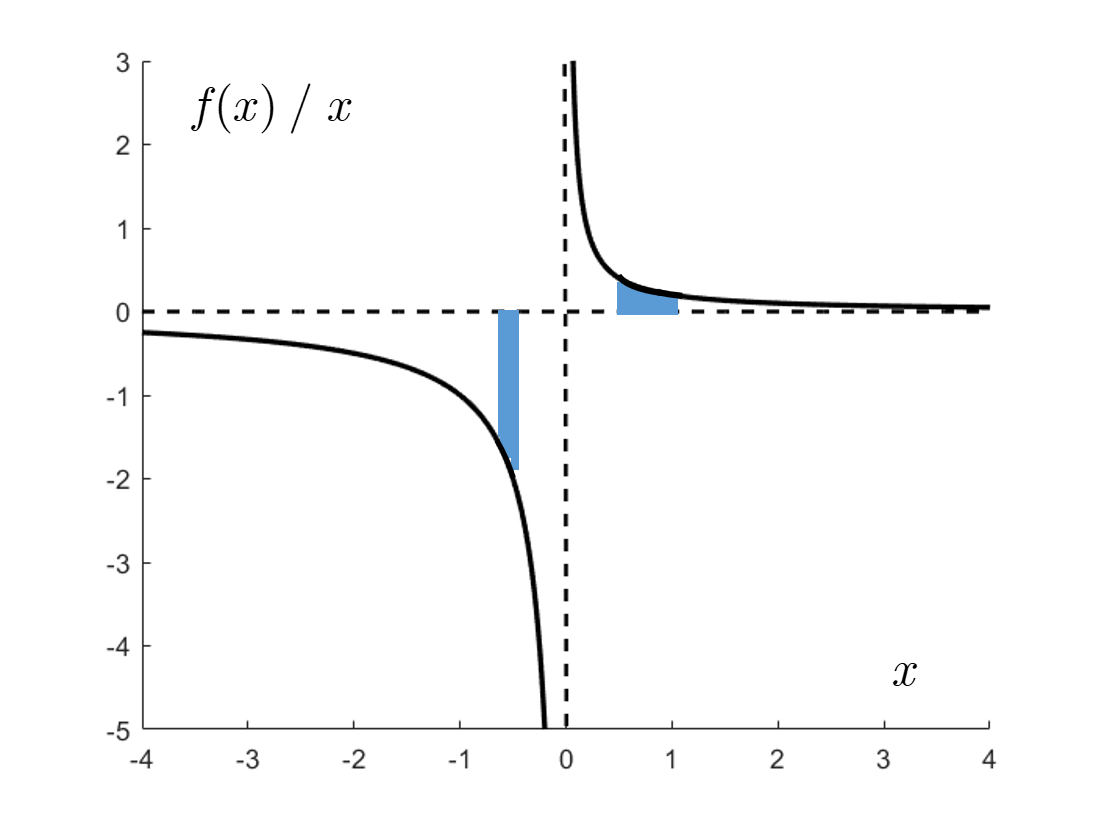
Figure 14: The principal value of the integral yields the true finite value of the net area under the curve $f(x)/x.$

The direct integration yields an indeterminacy of the form $\infty-\infty$:

$$\int_{x_{1}}^{x_{2}}\dfrac{f(x)}{x}dx=\int_{x_{1}}^{0}\dfrac{dx}{x}+\int_{0}^{x_{2}}\dfrac{dx}{5x}=\dfrac{1}{5}\ln x_{2}-\ln|x_{1}|\,+\infty-\infty.$$ (79)

However, the graphic in Fig. 14 suggests that the total area under the curve $f(x)/x$ might be finite, as the infinite negative area on the left seems to compensate for the infinite positive area on the right. Using the PV technique, we obtain

$$\wp\int_{x_{1}}^{x_{2}}\dfrac{f(x)}{x}dx=\lim_{\delta\rightarrow 0^{+}}\left[\int_{x_{1}}^{-\delta}\dfrac{dx}{x}+\int_{\delta}^{x_{2}}\dfrac{dx}{5x}\right]=\dfrac{1}{5}\ln x_{2}-\ln|x_{1}|,$$ (80)

as presumed.

We will now make use of the following relation:

$$\wp\int_{-\infty}^{\infty}\dfrac{\chi(\omega^{\prime})}{\omega^{\prime}-\omega}d\omega^{\prime}=i\pi\chi(\omega).$$ (81)

We have used the symbol $\chi$ because we are going to apply this result to the (linear) susceptibility, but (81) is a general mathematical property, valid for any function provided that it tends to zero when $|\omega|\,\rightarrow\infty.$ It is not by chance that this condition is indeed satisfied by the particular form (16) of $\chi(\omega)$; this regular behavior is actually based on physical grounds. We know that

$$\chi(\omega)=\int_{-\infty}^{\infty}\breve{\chi}(t)e^{-i\omega t}dt=\int_{0}^{\infty}\breve{\chi}(t)e^{-i\omega t}dt,$$ (82)

where the second equality follows from the causality of the dielectric response demanding $\breve{\chi}(t)=0$ for $t<0,$ as it was remarked with regard to (17). As it happens, the restriction $t>0$ in the integration of (82) is essential in the derivation of (81). If this were not the case, the contour integration mentioned in footnote 31 might diverge and the result (81) would not be generally ensured. In short, because causality guarantees the validity of (81), any physically acceptable (i.e., causal) susceptibility $\chi(\omega),$ regardless of its particular mathematical form, must satisfy the condition (81).

Separating the real and imaginary parts of $\chi$,

$$\chi(\omega)=\chi_{r}(\omega)+i\chi_{i}(\omega),$$ (83)

the expression (17) can be split in two equations:

$$\chi_{r}(\omega) =\dfrac{\wp}{\pi}\int_{-\infty}^{\infty}\dfrac{\chi_{i}(\omega^{\prime})}{\omega^{\prime}-\omega}d\omega^{\prime}$$ (84)

$$\chi_{i}(\omega) =-\dfrac{\wp}{\pi}\int_{-\infty}^{\infty}\dfrac{\chi_{r}(\omega^{\prime})}{\omega^{\prime}-\omega}d\omega^{\prime}.$$ (85)

Expressions (84)–(85) reveal a fundamental, unbreakable link between the dispersive behavior of a causal dielectric, described by $\chi_{r}(\omega)$, and its losses, described by $\chi_{i}(\omega).$ We note in passing that $\chi_{r}(\omega)$ and $\chi_{i}(\omega)$ are the Hilbert transform of each other [7].

The Kramers-Kronig (KK) relations [8] are just the equations (84)–(85) rewritten in an alternative form which involves the positive frequencies only. This is possible thanks to the real character of $\breve{\chi}(t),$ which implies that $\chi(\omega)$ satisfies the property (131) or, equivalently,

$$\chi_{r}(-\omega)=\chi_{r}(\omega)\text{\qquad and\qquad}\chi_{i}(-\omega)=\chi_{i}^{\ast}(\omega).$$ (86)

Splitting the integrals in (84)–(85) as $\int_{-\infty}^{\infty}=\int_{-\infty}^{0}+\int_{0}^{\infty}$ and using the symmetry properties (86), it is immediate to arrive at the following relations:

$$\chi_{r}(\omega) =-\dfrac{2}{\pi}\wp\int_{0}^{\infty}\dfrac{\omega^{\prime}\chi_{i}(\omega^{\prime})}{\omega^{2}-\omega^{\prime 2}}d\omega^{\prime}$$ (87)

$$\chi_{i}(\omega) =\dfrac{2\omega}{\pi}\wp\int_{0}^{\infty}\dfrac{\chi_{r}(\omega^{\prime})}{\omega^{2}-\omega^{\prime 2}}d\omega^{\prime}.$$ (88)

The KK relations (87)–(88) provide valuable insight into the form of the material response. For example, because the integral in (88) will generally be nonzero except at $\omega=0$, we cannot envision an hypothetical lossless dielectric if there is dispersion. In fact, if there existed a non-dispersive dielectric, i.e., one with $\chi_{r}(\omega^{\prime})=$ constant, then $\chi_{i}(\omega)=0$ (since $\wp\int_{0}^{\infty}(\omega^{2}-\omega^{\prime 2})^{-1}d\omega^{\prime}=0$) and the material would indeed be lossless in this case. Therefore, dispersion is necessarily associated to losses; since no medium other than vacuum is without dispersion, we find that a perfect transparent dielectric cannot exist.

As another example, it can be shown that if an isolated absorption peak exists at frequency $\omega_{0},$ then the real susceptibility in the quasi-transparent region near $\omega_{0}$ is of the form $\chi_{r}(\omega)\simeq B(\omega_{0}^{2}-\omega^{2})^{-1}$ [9]. This feature can be verified for $\chi_{r}(\omega)$ in the form (33), but it is a general result that follows from the KK relations without any mention to the particular physical origin or model of the absorption peak.

The KK relations also indicate that it is unnecessary to know both the real and imaginary parts of the susceptibility; the knowledge of one of them — albeit over the whole $0$ to $\infty$ frequency range — suffices to compute the other one. In fact, it is common-place to derive data of the real refractive index of a material from its absorption spectrum, which is usually easier to measure.

3.6 “Fast” and “slow” light

Early in the development and consolidation of the electromagnetic theory, it was realized that the formalism describing the propagation of waves might lead, apparently, to some bizarre results. This is readily seen when the expression of the group index (56) is replaced in (55), yielding

$$v_{g}(\omega)=\dfrac{c}{n(\omega)+\omega\dfrac{dn(\omega)}{d\omega}}.$$ (89)

Assuming that $n(\omega)$ $>0,$ one notices that if there is a frequency range with anomalous dispersion, this is, $dn(\omega)/d\omega<0$ ($dn_{\lambda}(\lambda)/d\lambda>0$), then the denominator of (89) might be smaller than 1, in which case we would have $v_{g}>c.$ The situation $dn_{\lambda}/d\lambda>0$ occurs indeed within the absorption peaks, as appreciated in Fig. 5. On the other hand, it should not be forgotten that expression (89) was derived assuming an almost transparent dielectric, which is obviously not the case in spectral regions with significant losses. Therefore, we must take a step back and check the validity of (89) for a complex $n(\omega).$

Writing $n(\omega)=n_{r}(\omega)-in_{i}(\omega),$ the propagation constant becomes complex:

$$k(\omega)=k_{R}(\omega)-ik_{I}(\omega)=(\omega/c)n_{r}(\omega)-i(\omega/c)n_{i}(\omega).$$ (90)

Following the same steps that led to (51), we arrive at the expression

$$\mathcal{\tilde{E}}(z,t)\simeq\frac{1}{2\pi}\int\nolimits_{-\infty}^{\infty}G(\Omega)\,e^{i[(\omega_{0}+\Omega)t-(k_{0}+k_{1}\Omega+\tfrac{1}{2}k_{2}\Omega^{2}+\cdots)z]\,}d\Omega.$$ (91)

But now all the coefficients $k_{j}$ of the Taylor expansion of $k(\omega)$ are complex. Writing $k_{j}=k_{jR}-ik_{jI},$ we have

$$\mathcal{\tilde{E}}(z,t)\simeq e^{i(\omega_{0}t-k_{0R}z)\,}e^{-k_{0I}z\,}\frac{1}{2\pi}\int\nolimits_{-\infty}^{\infty} G(\Omega)\,e^{i[\Omega(t-k_{1R}\Omega z)]\,}e^{-i\left(\tfrac{1}{2}k_{2R}\Omega^{2}z+\cdots\right)}$$

$$\times e^{-\left(k_{1I}\Omega+\tfrac{1}{2}k_{2I}\Omega^{2}+\cdots\right)}d\Omega.$$ (92)

It comes as no surprise that the presence of $k_{0I}=\operatorname{Im}k(\omega_{0})$ results in an exponential decay of the wave amplitude. In absence of the third exponential factor in the integrand, we would conclude that, apart from the global, non-distortive attenuation due to $k_{0I},$ the pulse would propagate as in the lossless case but with a group velocity $v_{g}=(dk_{1R}/d\omega)_{\omega=\omega_{0}}^{-1};$ i.e., expression (89) would apply with $n_{r}=\operatorname{Re}(n)$ in place of $n.$ Of course, some amount of distortion would be present, according to the values of $k_{2R},$ $k_{3R},$ etc. The key point is that the term $\exp[k_{1I}\Omega+(1/2)k_{2I}\Omega^{2}+\cdots]$ in (92) cannot be neglected. In our model, anomalous dispersion occurs precisely inside the absorption peaks, where losses are not only large, but also significantly dispersive, as shown in Fig. 15. Thus $k_{1I},$ $k_{2I}$, etc. cannot be ignored, which prevents drawing an analytical result of the form $\sim g(t-z/v_{g})$ from (92).

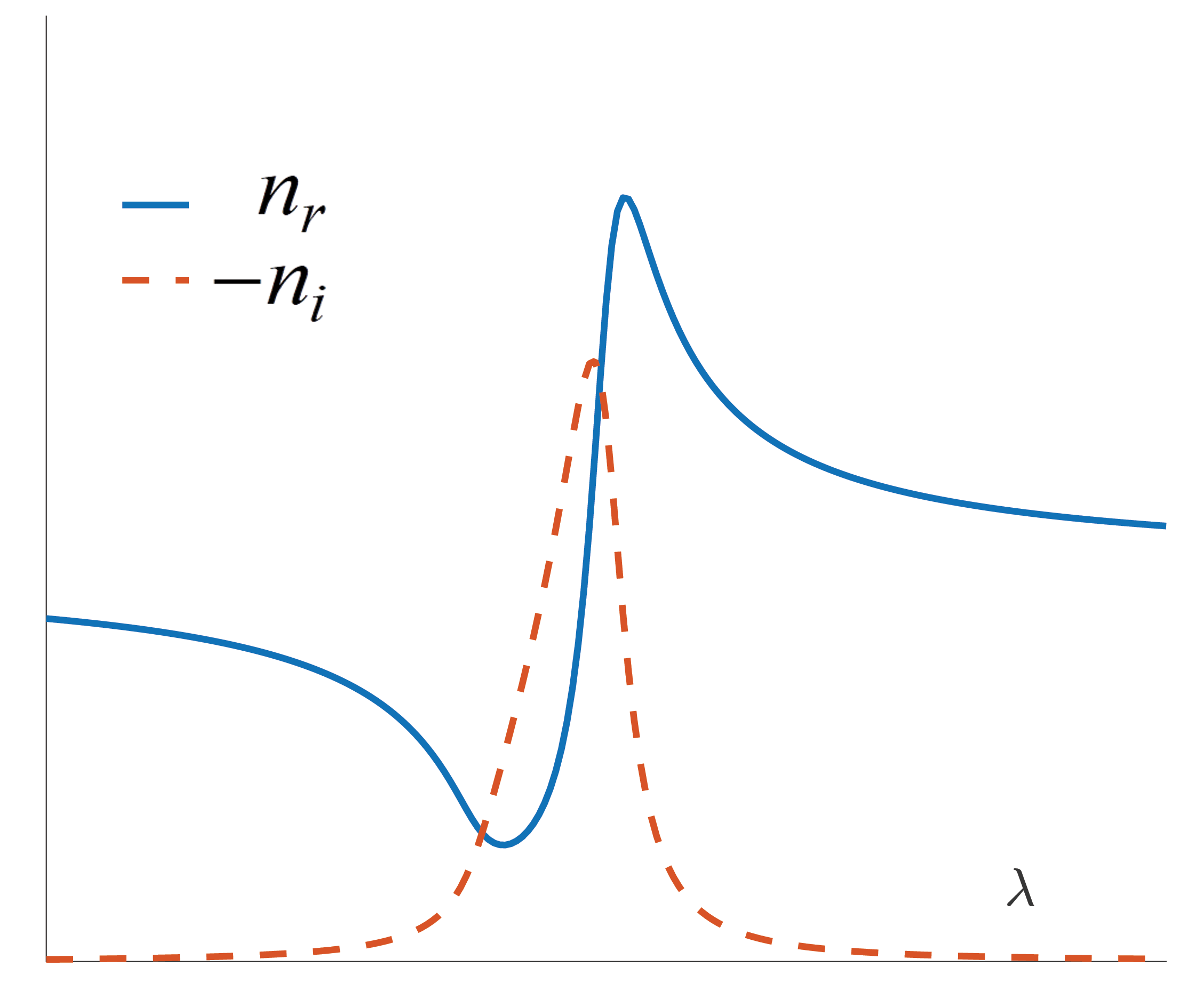
Figure 15: Real (blue) and imaginary (dashed red) parts of the refractive index around an isolated resonance. In a narrow spectral range there is anomalous dispersion.

One can insist on calling $v_{g}(\omega),$ as defined in (89) (with $n_{r}$ instead of $n$), the “group velocity” — and it is common practice —, but its meaning is not quite the same anymore. The fact that $v_{g}>c$ does not imply now that the wave envelope (the information) travels faster than light in vacuum, and there is of course not any affront to the special theory of relativity. Typically, the pulse becomes so attenuated and distorted (the latter being contributed not only by $n_{i}(\omega),$ but also by the strong dispersion of $n_{r}(\omega)$ around the resonances), that it can hardly be identified as an entity with a single propagation velocity. In any case, no portion of the arriving waveform travels faster than $c.$ In a better situation, when the pulse shape remains reasonably intact — even if severely attenuated —, the condition $v_{g}>c$ reflects the fact that the peak of the propagated pulse appears at the output when the peak of the input pulse has not yet entered the propagation section (see for example [10] and references therein). This phenomenon is useless to all practical purposes, however, as the pulse front never arrives before a time lapse $L/c$ has passed, $L$ being the propagation length.

There is no reason why $n_{g}$ could not even be negative. In one such situation, the pulse peak has been predicted to be moving backwards within the medium [11], a funny consequence of the peculiar interferences taking place during the propagation, but once again without any implication of the faster-than-light type.

From the corpuscular perspective, it seems quite obvious that the presence of any atomic media, dielectrics included, can never result in an effective velocity greater than $c.$ When photons are not interacting with matter, they can only be “flying” across the interatomic vacuum, naturally at speed $c.$ Absorptions and emissions, in turn, are processes that take time, so they can only but slow down the light travel further. In spite of these sensible objections, the misleading and somewhat pompous term “superluminal” has been coined and accepted to refer to any situation in which $v_{g}>c$ (or $n_{g}<1$). “Fast light” is another generic name sometimes used to refer to these phenomena.

A common type of superluminality is that arising in one-resonance absorbing atomic media as well as in artificial structures such as optical coupled resonators. This kind of superluminal propagation can be explained in a unified manner as an interference process [10]. Superluminality may occur in active (amplifying) media as well, in a manner rather similar to the absorption case. Other proposals make use of diverse nonlinear optical processes.

“Slow light” is another popular term. It refers to the ability of achieving very low group velocities. In this case, the condition $v_{g}<<c$ does represent a signal (typically a pulse) which propagates very slowly or, at least, at a velocity remarkable smaller than $c/n_{r}$, the phase velocity in the background material. Needless to say, the electromagnetic waves always propagate at speed $c,$ as discussed above; therefore, behind the expression “slow light” there is just a light-matter interaction process in an atomic medium which causes a particularly significant delay. In artificial structures, the delay is obtained basically by keeping the light going around a semi-closed path for as long as possible. Likewise, the also employed expression “stopped light” does not imply that a photon flux can been “stopped” at all, but simply means that the light is absorbed by a suitable medium which can remain excited indefinitely, and then re-emitted coherently at any desired time. (In the “meantime”, the energy and the information are stored in a different physical form inside the atomic medium; it is senseless to pretend that the absorbed and the re-emitted photons are “the same ones”.)

To a great extent, the research in slow light is aimed at developing optical retarders with high propagation delays over large spectral widths. Both requirements are hard to meet simultaneously. In fact, a theoretical limit to the maximum delay$\times$bandwidth product is often found in the basic types of the retarding structures (including bulk atomic media). In order to overcome these deeply-rooted limitations, nonlinear processes and other strategies are being explored (see for example [13]). Slow light — or, more generally, the control of the speed of light — has enormous applications in optical communications and optical (classical and quantum) processing in general [14].

4 Electromagnetism of linear amplifying media

By a simple extension of the results of Subsection 2.3, it is easy to model electromagnetically an optically amplifying material. For the sake of simplicity we will, again, consider plane waves propagating across an homogeneous, isotropic medium in the $z$ direction. Assuming a linearly polarized, purely monochromatic wave, the electric field has the form (31), which we reproduce here:

$$\mathcal{E}(z,t)=Ae^{-\,n_{i}(\omega_{0})(\omega_{0}/c)z}\cos\left(\omega_{0}t-n_{r}(\omega_{0})\frac{\omega_{0}}{c}z\right).$$ (93)

All that must be done for (93) to represent an amplified, rather than attenuated, wave propagating along the $+z$ direction, is to switch the sign of $n_{i}(\omega_{0})$ from positive to negative. In this way, (93) may describe an exponentially amplified wave, as illustrated in Fig. 16.

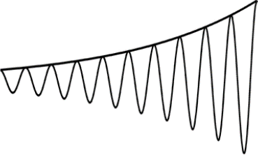
Figure 16: The graphic shows, for any fixed $t=t_{0},$ the form of the optical field $\mathcal{E}(z,t_{0})$ as it propagates along an amplifying medium having a refractive index with a negative imaginary part.

One can therefore say that, in order for a medium to amplify the light of frequency $\omega_{0},$ the imaginary part of its refractive index need be positive at that frequency, $-n_{i}(\omega_{0})>0.$ Apart from its usefulness by itself, optical amplification is essential to achieve laser oscillation. In Subsection 4.1 below, we will study in more detail the operation of the amplifier, while the fundamentals of the laser oscillation will be briefly presented in Subsection 4.2.

4.1 Dielectric susceptibility and population inversion

We assume that the susceptibility of a dielectric, whether passive or active (amplifying), can be written as in (33),

$$\chi(\omega)=\sum\limits_{j=1}^{N}\frac{A_{j}\,\omega_{j}^{2}}{-\omega^{2}-i\omega\,b_{j}+\omega_{j}^{2}}.$$ (94)

We further assume that the radiation frequency $\omega$ is far from all the resonance frequencies of the material but one, $\omega_{r},$ so that

$$\chi(\omega)\simeq\sum\limits_{j\neq r}^{N}\frac{A_{j}\,\omega_{j}^{2}}{\omega_{j}^{2}-\omega^{2}}+\frac{A_{r}\,\omega_{r}^{2}}{-\omega^{2}-i\omega\,b_{r}+\omega_{r}^{2}}\equiv\bar{\chi}(\omega)+\chi_{\text{res}}(\omega)\qquad\text{(near }\omega_{r}\text{),}$$ (95)

where $\bar{\chi}(\omega),$ including all the terms in the parenthesis in (95), is the (real-valued) “non-resonant” susceptibility, and

$$\chi_{\text{res}}(\omega)=\frac{A_{r}\,\omega_{r}^{2}}{-\omega^{2}-i\omega\,b_{r}+\omega_{r}^{2}}\equiv\chi^{\prime}(\omega)-i\chi^{\prime\prime}(\omega),$$ (96)

which describes the effect of the resonant transition at $\omega_{r}$ on the propagating wave. We next define the “background index”,

$$\bar{n}(\omega)\equiv\sqrt{1+\bar{\chi}(\omega)},$$ (97)

which can be thought of as the (real-valued) refractive index, at frequencies near $\omega_{r},$ contributed by all other resonances (Fig. 5). The actual refractive index near the resonance can then be expressed as follows:

$$n(\omega) =\sqrt{1+\chi(\omega)}\simeq\sqrt{1+\bar{\chi}(\omega)+\chi^{\prime}(\omega)-i\chi^{\prime\prime}(\omega)}=\bar{n}(\omega)\sqrt{1+\dfrac{\chi^{\prime}(\omega)-i\chi^{\prime\prime}(\omega)}{\bar{n}^{2}(\omega)}}$$

$$\simeq\,\bar{n}(\omega)\left(1+\dfrac{\chi^{\prime}(\omega)}{2\bar{n}^{2}(\omega)}\right)-i\dfrac{\chi^{\prime\prime}(\omega)}{2\bar{n}(\omega)}\equiv n_{r}(\omega)-in_{i}(\omega)\qquad\text{(near }\omega_{r}\text{)}$$ (98)

if $|\chi_{\text{res}}(\omega)|/\bar{n}^{2}(\omega)<<1$.

The effect of the resonance is twofold. On one hand, it slightly modifies $\bar{n}(\omega)$ through $\chi^{\prime}(\omega)$; on the other, it brings about an imaginary part $-n_{i}(\omega)$ which will cause attenuation or amplification, depending on its sign. Actually, the classical intensity (W/m²) of this monochromatic plane wave propagating through a dielectric medium of index $n=n_{r}-in_{i}$ is given by by the well-known expression

$$I_{\text{Cl}}=\sqrt{\frac{\epsilon_{0}}{\mu_{0}}}n_{r}|\tilde{E}(z)|^{2},$$ (99)

with $\tilde{E}(z)$ the complex amplitude or phasor of the field (93),

$$\widetilde{E}(z)=Ae^{-\,n_{i}(\omega)\frac{\omega}{c}z}e^{-\,in_{r}(\omega)\frac{\omega}{c}z}.$$ (100)

Replacing (100) in (99), we obtain

$$I_{\text{Cl}}=\sqrt{\frac{\epsilon_{0}}{\mu_{0}}}n_{r}A^{2}\exp\left[-2\dfrac{\omega}{c}n_{i}(\omega)z\right],$$ (101)

which will grow along the propagation direction $z$ as long as $-n_{i}(\omega)>0.$

Now, what is the physical origin of a positive refractive index (negative $n_{i}$)? In principle, a quantum-mechanical model of the electromagnetic radiation would be necessary to answer this question. Without going that far, Einstein’s model for the interaction between light and two-level atoms provides sufficient insight for our purposes. We will basically follow a rather standard derivation such as that presented in [15]. We call $N_{1}$ and $N_{2}$ the average atomic density (atoms/m³) of atoms (or molecules) in the ground state (energy $E_{1}$) and excited state (energy $E_{2}>E_{1}$), respectively. The energy of the photons must match the atomic energy difference: $E_{2}-E_{1}\approx h\nu_{r}=\hbar\omega_{r}.$ $N_{1}$ and $N_{2}$ will generally depend of the specific site within the material (i.e. they are functions of $z$), but for low optical intensity (“small signal”) they can be considered approximately constant. We will not elaborate further on this model, which can be found in countless textbooks of photonics and related fields. Assuming our (dielectric) material is made up of such two-level atoms or molecules, the optical intensity is found to evolve according to the expression

$$I=I(0)\exp[\sigma_{\nu}(N_{2}-N_{1})z]\,\qquad\text{(valid for small signal).}$$ (102)

In (101), $\sigma_{\nu}$ is the so-called cross-section, which depends on the properties of the material and on the frequency $\nu.$ Namely,

$$\sigma_{\nu}=\frac{c^{2}}{8\pi\bar{n}^{2}\nu^{2}\tau_{\text{sp}}}\bar{g}(\nu)$$ (103)

with $\tau_{\text{sp}}$ the spontaneous emission time (the average time it takes an excited atom at level $E_{2}$ to spontaneously deexcite to level $E_{1}$ by emitting a photon of energy $E_{2}-E_{1},$ with random direction and phase). In (103), $\bar{g}(\nu)$ is the normalized ($\int_{0}^{\infty}$ $\bar{g}(\nu)d\nu=1$) spectral lineshape or lineshape function, which has a probabilistic interpretation: roughly speaking, $\bar{g}(\nu)d\nu$ is the probability that a photon having an energy between $\nu$ and $\nu+d\nu$ will be emitted/absorbed by the atom, if an emission/absorption is to occur. The simplest form of $\bar{g}(\nu)$ is the so-called Lorentzian lineshape (Fig. 17):

$$\bar{g}(\nu)=\frac{1}{2\pi}\frac{\Delta\nu}{(\nu-\nu_{r})^{2}+(\Delta\nu/2)^{2}},$$ (104)

peaked at $\nu=\nu_{r}.$

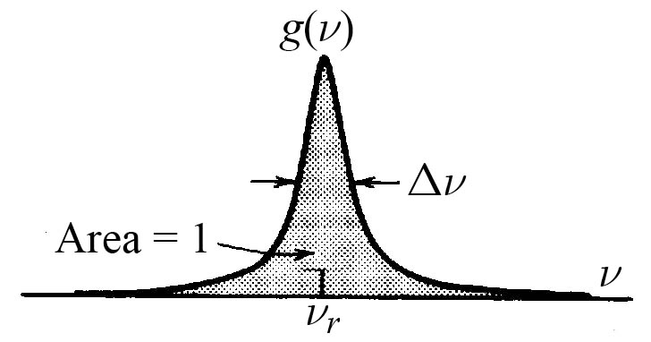
Figure 17: Lorentzian lineshape around the central frequency $\nu_{r}.$

Note that (101) is also a “small signal” result, like (102), since it was derived within the framework of linear optics, thus excluding nonlinear phenomena such as gain saturation or others.

Expressions (101) and (102) should then be equivalent, which demands that the exponents be equal. Recalling (103), this leads to

$$n_{i}=-\frac{1}{\tau_{\text{sp}}}\frac{c^{3}}{32\pi^{2}\bar{n}^{\,2}\nu^{3}}\bar{g}(\nu)(N_{2}-N_{1}).$$ (105)

Formula (105) shows the connection between the imaginary part of the refractive index and the “quantum state” of the atoms of the material. An amplifying medium requires $n_{i}<0,$ hence $N_{2}>N_{1}$ — there must exist population inversion in the medium, i.e. more atoms in the excited state than in the ground state.

Near the resonance at $\nu_{r}=$ $\omega_{r}/(2\pi),$ some frequency-dependent parameters in (105) can be considered practically constant within the whole narrow linewidth span $\Delta\nu$; namely, $\nu^{3}\simeq\nu_{r}^{3}$ and $\bar{n}^{\,2}(\nu)\simeq\bar{n}^{\,2}(\nu_{r})$ (recall that $\bar{n}$ excludes the resonance peak at $\nu_{r}$). Thus the frequency dependence of $n_{i}$ is essentially given by the Lorentzian line $\bar{g}(\nu)$ (104), which does display an abrupt variation. The linewidth $\Delta\nu$ can typically be of the order of hundreds of GHz. Of course, $n_{i}$ given in (98) should have the same Lorentzian form. Let us check this. Computing $\chi^{\prime\prime}=-\operatorname{Im}(\chi_{\text{res}}),$ we obtain

$$n_{i} \simeq\dfrac{\omega_{r}}{8\bar{n}(\omega_{r})}\frac{A_{r}b_{r}}{(\omega-\omega_{r})^{2}+b_{r}^{2}\omega_{r}^{2}/4}\text{\qquad\ [}\omega\text{ (}\nu\text{) near }\omega_{r}\text{ (}\nu_{r}\text{)]}$$ (106)

$$=\text{sign}[A_{r}]\dfrac{\nu_{r}}{8\bar{n}(\nu_{r})}\frac{1}{2\pi}\frac{\Delta\nu}{(\nu-\nu_{r})^{2}+(\Delta\nu/2)^{2}}=\text{sign}[A_{r}]\dfrac{\nu_{r}}{8\bar{n}(\nu_{r})}\bar{g}(\nu).$$ (107)

The approximations $\omega_{r}^{2}-\omega^{2}=(\omega_{r}+\omega)(\omega_{r}-\omega)\simeq 2\omega_{r}(\omega_{r}-\omega),$ $\omega^{2}\simeq\omega_{r}^{2}$ and $\bar{n}^{\,2}(\omega)\simeq\bar{n}^{\,2}(\omega_{r})$ have been used in (106). All are justified by the assumption that $\omega$ is close to $\omega_{r}$ within a range of the order $\Delta\omega=2\pi\Delta\nu<<\omega_{r},$ as stated above. In this way, (105) and (106)–(107) are consistent as they have the same Lorentzian frequency dependence. We also see that the relation $\Delta\nu$ $=|A_{r}|b_{r}$ must hold, in the understanding that $A_{r}$ will be negative in an amplifying material.

A useful expression showing explicitly the frequency dependence of $\chi^{\prime\prime}$ can be obtained from the first equality in (106) and (105), again with $\nu^{3}\simeq\nu_{r}^{3}$ and calling $\lambda_{r}=c/\nu_{r},$ the resonance (vacuum) wavelength:

$$\chi^{\prime\prime}(\nu) =\frac{1}{\tau_{\text{sp}}}\frac{c^{3}}{16\pi^{2}\bar{n}(\nu_{r})^{\,}\nu_{r}^{3}}\bar{g}(\nu)(N_{1}-N_{2})$$

$$=\frac{\lambda_{r}^{3}}{8\pi^{3}\bar{n}(\lambda_{r})\tau_{\text{sp}}^{\,}\Delta\nu}\frac{N_{1}-N_{2}}{1+\left(\dfrac{\nu-\nu_{r}}{\Delta\nu/2}\right)^{2}}\text{\qquad(near }\nu_{r}\text{).}$$ (108)

It is easy to check that $\chi^{\prime}(\nu)$ is related to $\chi^{\prime\prime}(\nu)$ through the simple expression

$$\chi^{\prime}(\nu)=2\frac{\nu_{r}-\nu}{\Delta\nu}\chi^{\prime\prime}(\nu).$$ (109)

4.2 Laser oscillation

In the preceding subsection we have explored how a suitable dielectric material can be turned into an optical amplifier. Amplification is indeed the first requirement to make a laser, but some mechanism providing output-to-input feedback must be added in order to obtain optical oscillation. Not surprisingly, the most straightforward way to achieve signal feedback at optical frequencies is to use mirrors. The basic structure is shown in Fig. 18. The active dielectric medium is confined between two partially reflecting plane mirrors separated by a distance $L$. Calling $R_{1}$ and $R_{2}$ the power reflectivities of the mirrors ($R_{1}\leq 1,$ $R_{2}<1$), the fraction of the field amplitude reflected at each end will be$\sqrt{R_{1}}$ and $\sqrt{R_{2}},$ respectively, for a plane wave propagating in the $\pm z$ direction, as assumed. Such a structure is called a Fabry-Pérot (FP) cavity.

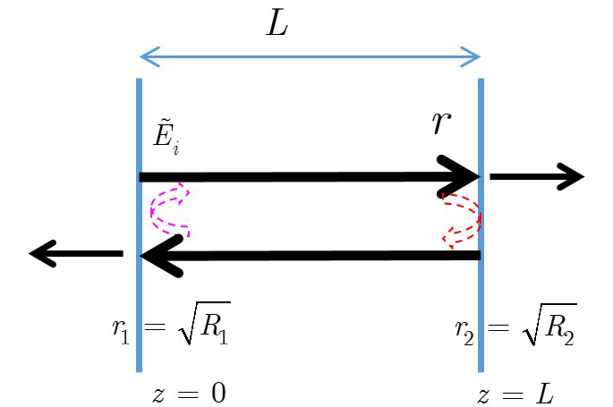
Figure 18: A Fabry-Pérot laser. The cavity between the mirrors is filled with a dielectric material that can be made to amplify the light.

Roughly speaking, a self-maintained electromagnetic oscillation will occur if the amplification of the light within the cavity compensates for all the propagation losses. Assume that a monochromatic wave exists inside the FP cavity with an amplitude $E_{1}$ at, for example, $z=0,$ immediately to the right of mirror 1 (any other $z$ location could be chosen). The existence of such a wave across the structure is only possible if the following consistency condition is fulfilled:

$$E_{1}e^{-i\tilde{k}L}\sqrt{R_{2}}e^{-i\tilde{k}L}\sqrt{R_{1}}=E_{1},$$ (110)

with

$$\tilde{k}=\frac{\omega_{L}}{c}n(\omega_{L})=\frac{\omega_{L}}{c}[n_{r}(\omega_{L})-in_{i}(\omega_{L})]\equiv k(\omega_{L})-ik_{i}(\omega_{L}),$$ (111)

the complex propagation constant, where $\omega_{L}$ is the angular wave frequency, still unknown but assumed to be close to $\omega_{r}.$ On the LHS of (110), $E_{1}e^{-i\tilde{k}L}=(E_{1}e^{-k_{i}L})e^{-ikL}\equiv\tilde{E}_{2}$ simply describes the amplitude and phase of a right-propagating wave at $z=L$ (just before mirror 2) if, as assumed, it has a real amplitude $E_{1}$ at $z=0.$ A reflected wave must then exist with an amplitude $\tilde{E}_{2}\sqrt{R_{2}}\equiv\tilde{E}_{3}$ at $z=L$ (it is assumed that the mirrors do not introduce any phase shift). The field of this backward-propagating wave will necessarily be $\tilde{E}_{3}e^{-i\tilde{k}L}\equiv\tilde{E}_{4}$ at $z=0,$ and $\tilde{E}_{4}\sqrt{R_{1}}\equiv\tilde{E}_{5}$ immediately after reflection at $z=0,$ where it is identified with the assumed right-propagating field we started with, i.e. $\tilde{E}_{5}=E_{1}.$ This gives the result (110). Equating modulus and phase separately, (110) yields

$$\sqrt{R_{1}R_{2}}e^{-2k_{i}L} =1\qquad\qquad\qquad\qquad\text{(modulus)}$$ (112)

$$kL =m\pi,\quad m=1,2,\ldots\quad\text{(phase).}$$ (113)

We will consider the modulus condition first. Using (98) in (111), we get

$$\tilde{k}(\omega_{L})=k(\omega_{L})-ik_{i}(\omega_{L})=\frac{\omega_{L}}{c}\bar{n}(\omega_{L})\left(1+\dfrac{\chi^{\prime}(\omega_{L})}{2\bar{n}^{2}(\omega_{L})}\right)-i\left(\frac{\omega_{L}}{c}\dfrac{\chi^{\prime\prime}(\omega_{L})}{2\bar{n}(\omega_{L})}+\dfrac{\alpha_{\text{int}}}{2}\right).$$ (114)

The extra term $-i\alpha_{\text{int}}/2$ has been introduced ad hoc to account for additional propagation losses which are difficult to model electromagnetically in a rigorous fashion. For example, diffraction losses cannot possibly arise in our idealized one-dimensional model supporting plane waves of infinite extent, but they do exist in real devices. Other contributions to $\alpha_{\text{int}}$ may include polarization losses, scattering losses, etc.

Using (114) in (112) leads to

$$g(\omega_{L})=\alpha_{m}+\alpha_{\text{int}},$$ (115)

with

$$g(\omega_{L})\doteq-\frac{\omega_{L}}{c}\dfrac{\chi^{\prime\prime}(\omega_{L})}{\bar{n}(\omega_{L})},$$ (116)

the material gain, and

$$\alpha_{m}\doteq\frac{1}{2L}\ln\frac{1}{\sqrt{R_{1}R_{2}}},$$ (117)

the mirror losses. The latter accounts for the radiation escaping through the mirrors. Obviously, if both mirrors were perfectly reflecting ($R_{1}=R_{2}=1$), then $\alpha_{m}=0,$ but in this case the laser would be useless; at least one of the mirrors must be partially reflecting to let some light out.

The material gain $g$ (not to be confused with the lineshape function $\bar{g}$) will be positive if $\chi^{\prime\prime}<0,$ which according to (108) demands the material to be in population inversion, this is, $N_{2}>N_{1}.$ In this case, the interpretation of condition (115) is clear: maintaining a sustained optical wave in the resonator requires that the amplification of the active medium compensate exactly for all the propagation losses in the cavity, including of course the energy lost through the mirrors. Generally, one of the mirrors is almost perfectly reflecting ($R_{1}\simeq 1$) while the other provides the output. Laser diodes are a remarkable exception as both mirrors radiate equally.

No situation other than (115) permits self-sustained oscillation. If an initial oscillation is assumed to exist in the cavity but the gain is smaller than the losses, the radiation will extinguish after a few round-trips. On the other hand, if the gain were larger than the losses, the optical field would increase in each round-trip, approaching an infinite value. Such a situation cannot be physically envisioned and, more precisely, gain saturation is the mechanism which prevents such phenomenon from taking place, as we will discuss later.

Gain is one half of the story. Even if the field “returns” to the same point of the cavity with the same intensity, it also needs to have the same phase; otherwise, destructive interference would prevent the oscillation. Using (114) in the phase condition (112) leads to an implicit expression for the set of potential lasing frequencies $\omega_{L}\in\{\omega_{m}\}$:

$$\nu_{m}=\frac{\omega_{m}}{2\pi}=\frac{mc}{2\bar{n}(\omega_{m})\left(1+\dfrac{\chi^{\prime}(\nu_{m})}{2\bar{n}^{2}(\nu_{m})}\right)L},\qquad m=1,2,\ldots$$ (118)

Note that, if the active resonance could be removed from the cavity material, then $\chi^{\prime}=0$ and (118) would reduce to

$$\tilde{\nu}_{m}=\frac{mc}{2\bar{n}(\tilde{\nu}_{m})L},\qquad m=1,2,\ldots\qquad\text{(cavity of real index }\bar{n}\text{, no }\nu_{r}\text{ resonance),}$$ (119)

where we have renamed the resulting oscillation frequencies in this case as $\tilde{\nu}_{m}$ ($\tilde{\omega}_{m}=2\pi\tilde{\nu}_{m}$). From (109) and (108), $\chi^{\prime}(\nu)=0$ when $N_{2}=N_{1}.$ The frequencies $\tilde{\nu}_{m}$ are sometimes called the “cold cavity” resonant frequencies or modes. Expression (118) can then be rewritten as

$$\nu_{m}=\frac{\tilde{\nu}_{m}}{1+\dfrac{\chi^{\prime}(\nu_{m})}{2\bar{n}^{2}(\nu_{m})}},\qquad m=1,2,\ldots$$ (120)

Formula (109) shows that, if an actual oscillation frequency $\nu_{m}$ turns out to be equal to the actual material resonance frequency, $\nu_{r}$, then $\chi^{\prime}(\nu_{m})=0$ for any value of the population inversion $N_{2}-N_{1},$ in which case $\nu_{m}=\tilde{\nu}_{m}=\nu_{r}.$ In other words, when the center frequency of the atomic line $\bar{g}(\nu)$ coincides with one of the “cold cavity” modes, the frequency of this cavity mode will be the actual lasing frequency. In any other case, $\chi^{\prime}(\nu_{m}),$ even if not zero, is expected to be small if $\nu_{m}$ is very close to $\nu_{r}$ [c.f. (109)], in which case the correction will be small. A detailed analysis shows that the presence of $\chi^{\prime}$ tends to shift $\nu_{m}$ slightly from $\tilde{\nu}_{m}$ toward $\nu_{r},$ leading to the so-called frequency-pulling [15], [16].

We will now explain the operation of the laser graphically. First, ignoring the effect of $\chi^{\prime}$ for simplicity, expression (119) seems to suggest that the possible oscillation frequencies, represented as vertical lines in Fig. 19, are equispaced with a separation $c/(2\bar{n}L)$ between two adjacent “lines”. This is not exactly the case as $\bar{n}$ is not constant but frequency-dependent itself. A more accurate result is obtained as explained next.

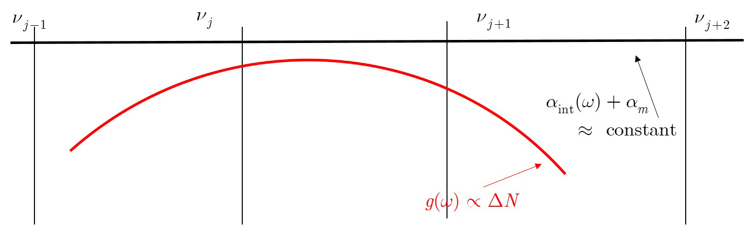
Figure 19: Spectral loss (black) and gain (red) curves of the cavity. Some possible oscillation frequencies of the laser (assumed to be in the vicinity of the atomic transition $\nu_{r}$) are also indicated. The red arc could represent, for example, the peak of the Lorentzian curve shown in Fig. 17. In the case depicted, there is no (or not enough) population inversion $\Delta N=N_{2}-N_{1}.$ Thus, the net loss exceeds the net loss at all frequencies and the cavity will not lase.

Expression (119) can be rewritten as $\tilde{\nu}_{m}\,\bar{n}(\tilde{\nu}_{m})=mc/(2L).$ In particular, calling $\delta\tilde{\nu}$ the frequency step, i.e. $\tilde{\nu}_{m+1}=\tilde{\nu}_{m}+\delta\tilde{\nu},$ and writing $\bar{n}(\tilde{\nu}_{m+1})=\bar{n}(\tilde{\nu}_{m}+\delta\nu)=\bar{n}(\tilde{\nu}_{m})+\delta\bar{n},$ the equality reads, for $m+1,$

$$(\tilde{\nu}_{m}+\delta\nu)(\bar{n}(\tilde{\nu}_{m})+\delta\bar{n})=(m+1)\frac{c}{2L}=\tilde{\nu}_{m}\,\bar{n}(\tilde{\nu}_{m})+\frac{c}{2L},$$ (121)

Neglecting the 2nd-order infinitesimal $\delta\tilde{\nu}\delta\bar{n},$ (121) simplifies to

$$\tilde{\nu}_{m}\delta\bar{n}+\bar{n}(\tilde{\nu}_{m})\delta\nu=\frac{c}{2L}\Longrightarrow\left[\tilde{\nu}_{m}\left.\frac{\partial\bar{n}}{\partial\nu}\right|_{\tilde{\nu}_{m}}+\bar{n}(\tilde{\nu}_{m})\right]\delta\nu=\frac{c}{2L}.$$ (122)

Recognizing the expression of $\bar{n}_{g}(\tilde{\nu}_{m})$, the group index, in the square brackets, we finally obtain

$$\delta\nu=\frac{c}{2\bar{n}_{g}L}\qquad\text{(ignoring }\chi^{\prime}\text{ frequency pulling).}$$ (123)

If the background group index $\bar{n}_{g}$ remains reasonably constant in the spectral range of interest, near $\nu_{r},$ the oscillation frequencies will be equispaced.

Let us examine the compliance of equality (115). Regardless of the population inversion $N_{2}-N_{1}$, which being a constant simply determines the peak amplitude of the gain curve, the shape of $g(v)$ will be Lorentzian, as stated. However, the right-hand term of (115) is essentially flat. Even if both $\alpha_{\text{int}}$ and $\alpha_{m}$ are really frequency-dependent (for example, the reflectivities $R_{1}$ and $R_{2}$ obviously depend on the wavelength), they can be considered very approximately constant within the narrow spectral width of interest. The situation is illustrated schematically in Fig. 20. Consider that the material is at first unpumped, so that $N_{1}-N_{2}>0$ ($g(\nu)$ is represented by the solid blue curve) and the light could only experiment attenuation. In this case, $g(\nu)<\alpha_{m}+\alpha_{\text{int}}$ at all frequencies and of course there is no oscillation. Next, we enable the pumping, thus increasing $N_{2}-N_{1}$ to the point that $g(\nu)$ (brown solid line) surpasses the losses within some frequency range. However, none of the permitted, phase-adapted oscillation frequencies lies in this range, so still no oscillation can arise. Increasing $N_{2}-N_{1}$ further, the situation is finally reached where $g$ equals $\alpha_{m}+\alpha_{\text{int}}$ (the gain threshold value) at one of the eligible frequencies (green thick solid line). Lasing will then start at that specific frequency only (at least in our simple description).

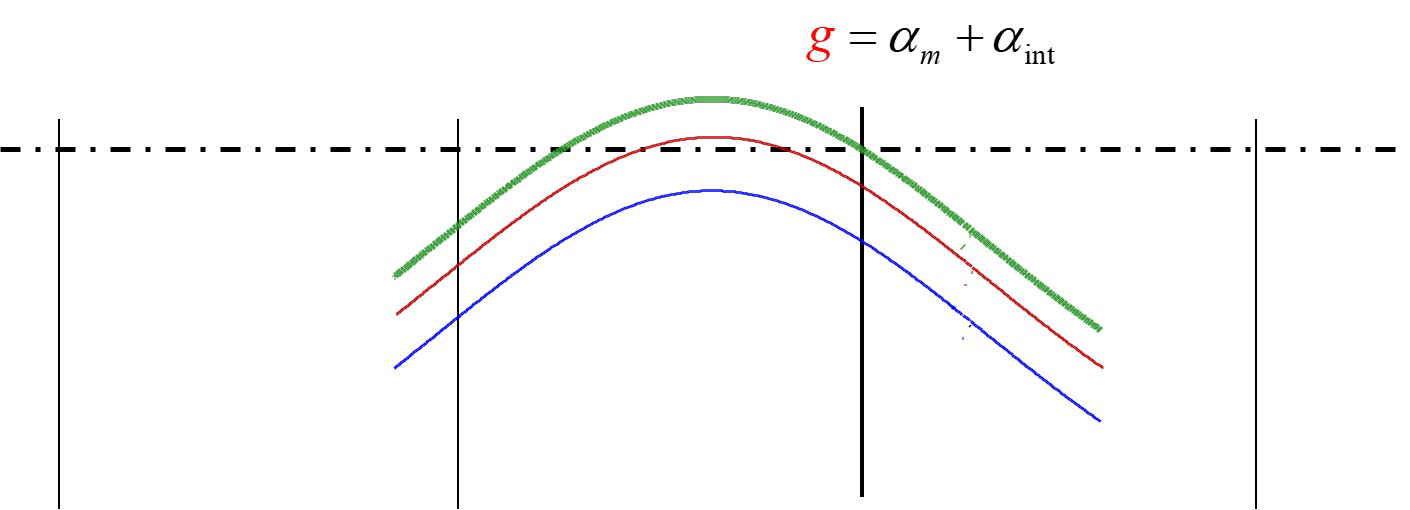
Figure 20: Increased pumping ends up creating sufficient population inversion to build up a laser oscillation at one of the possible frequencies. See text.

One may wonder how the oscillation actually builds up if there was no light in the cavity in the first place. Just as an electronic oscillator is started by the electronic noise existing the circuit, optical oscillation in a laser is triggered by some photon generated by spontaneous emission stemming from the fraction of atoms in the cavity which have been thermically excited to the upper energy level. It is only necessary, and statistically feasible, for one single so-emitted photon to have the suitable direction and phase to match the modal characteristics of the waves propagating in the cavity (an ideal, unphysical plane wave pattern in our discussion, but a real specifically shaped optical beam or waveguide mode in actual lasers).

What happens if the pumping is increased beyond the threshold value? In principle, $N_{2}-N_{1}$ should increase accordingly but, as remarked above, such a situation cannot endure since the field intensity inside the cavity grows to saturate the gain almost immediately. This will necessarily end up occurring even if $g$ is only “infinitesimally” greater $\alpha_{m}+\alpha_{\text{int}}$ (or, equivalently, $N_{2}-N_{1}$ “infinitesimally” greater than the threshold value of $N_{2}-N_{1}$). The mechanisms involved can be qualitatively described as follows.

(a) At threshold, the photons generated by stimulated emission from the net inverted atom population ($N_{2}-N_{1}$) are “used up” to balance the cavity round-trip losses.

(b) If pumping is increased, more atoms are lifted to the excited state ($N_{2}-N_{1}$ increases), which will boost the stimulated emission rate within the cavity. The new photons will quickly induce still more stimulated emissions, producing more photons which will in turn trigger further emissions, and so on. Now, for each emitted photon, $N_{2}-N_{1}$ decreases by two units. The photon emission rate, which grows dramatically, will very quickly surpass the fixed pumping rate, so the photons in the cavity will soon significantly outnumber the existing excited atoms. At this point, most of these photons cannot stimulate emissions any more simply because there are no more excited atoms available. This is, of course, nothing but a gain saturation process ($N_{2}-N_{1}$ decreases, so the gain does too). From an electromagnetic point of view, this process can be formally accounted for by using a saturable, intensity-dependent dielectric susceptibility in the model, rather than (94); we will not pursue this topic further.

(c) Now, all these newly-created photons will necessarily be evacuated through the mirrors (not through the losses $\alpha_{\text{int}},$ which are already “fed” by the photons generated at the threshold value pumping).

(d) If the pumping could then be swiftly switched back to the threshold value, an hypothetical observer would have simply seen a “light burst” corresponding to the transient exiting photons. However, if the pumping above threshold is maintained, photons in excess will be continuously created at a steady rate. These will be constantly escaping through the mirrors. Meanwhile, as explained, the photon density inside the cavity in steady state can only remain “clamped” to its threshold value (115) — the only stable value — regardless of the level of the “excess” pumping rate. As a side note, it must be kept in mind that, even at the threshold level, the gain may be significantly saturated (see footnote 37). Hence $g$ in equality (115) might not be well represented by the “small signal” gain and a full intensity-dependent expression for $g$ might have to be employed, as mentioned above.

(e) Although the level of (above-threshold) pumping does not have any effect on the equilibrium condition inside the cavity, we see that it has an important effect: it generates a surplus of photons that are radiated out. The higher the pumping rate is, the more photons will have to leave the cavity. In other words, once the threshold gain has been reached, all additional pumping will be used to generate more optical power.

The quantitative analysis of the operation and optimization of the emitted laser power (where the reflectivity of the output mirror plays a key role) can be found in innumerable textbooks.

Appendix A APPENDIX on the Fourier transform and a few closely related topics

Throughout these notes we consistently use the following definition for the time-frequency Fourier transform pair:

$$\mathcal{G}(t) =\frac{1}{2\pi}\int_{-\infty}^{\infty}G(\omega)\,e^{i\omega t}d\omega$$ (124)

$$G(\omega) =\int_{-\infty}^{\infty}\mathcal{G}(t)\,e^{-i\omega t}dt.$$ (125)

Here $\omega$ is the angular frequency in radians, related to the ordinary frequency $\nu$ in hertzs by $\omega=2\pi\nu.$ Unfortunately, there exist quite a few different (albeit equivalent) conventions to define the transform pair in the literature. For example, the factor $(2\pi)^{-1}$ can appear as a prefactor in (125) instead of (124), or as $(2\pi)^{-1/2}$ in both. The signs $\pm$ in front of the exponent $i\omega$ in the integrals are also a matter of taste. The choice (124)–(125) is frequently used in electrical engineering texts, while in the physics literature the signs often appear exchanged. As a consequence, the propagation factor of a monochromatic electromagnetic wave travelling in the $+z$ direction will read $\exp[i(\omega t-\beta z)]$ with our definition, instead of the alternative form $\exp[i(\beta z-\omega t)]$. In order to adapt one convention to the other, it will generally suffice to substitute $i\rightarrow-i$ throughout.

A.1 Some basic properties

Here we only quote those properties of the Fourier transform (FT) which are occasionally used in these notes. Apart from the linearity, it is very easy to prove the following:

$$\text{FT}\left\{\frac{d^{n}}{dt^{n}}\mathcal{G}(t)\right\} =(i\omega)^{n}G(\omega)$$ (126)

$$\text{FT}\{(-it)^{n}\mathcal{G}(t)\} =\frac{d^{n}}{d\omega^{n}}G(\omega)$$ (127)

$$\text{FT}\left\{\mathcal{G}(t-t_{0})\right\} =e^{-i\omega t_{0}}G(\omega)$$ (128)

$$\text{FT}\left\{e^{i\omega_{0}t}\mathcal{G}(t)\right\} =G(\omega-\omega_{0})$$ (129)

$$\text{FT}\left\{\mathcal{G}(at)\right\} =\frac{1}{|a|}G\left(\frac{\omega}{a}\right)\qquad\text{(scaling).}$$ (130)

If $\mathcal{G}(t)$ is real, then

$$G(\omega)=G^{\ast}(-\omega)\qquad\text{(}\mathcal{G}(t)\text{ real),}$$ (131)

which follows readily using (124) and forcing $\mathcal{G}(t)=\mathcal{G}^{\ast}(t).$

Writing $G(\omega)$ in the Euler form, $G(\omega)=|G(\omega)|\exp[i\gamma_{G}(\omega)],$ (131) implies that the modulus $|G(\omega)|$ is an even function of $\omega$ while the phase $\gamma(\omega)$ is odd. In the case of a linear, single-mode optical fiber of length $L$ with negligible losses, a fiber transfer function $H(\omega)=|H(\omega)|\exp[i\gamma_{H}(\omega)]$ can be defined with $|H(\omega)|\simeq 1$ and $\gamma_{H}(\omega)=-\beta(\omega)L$, where $\beta(\omega)$ is the propagation constant of the field, which can be written as $\beta(\omega)=(\omega/c)\bar{n}(\omega),$ $\bar{n}(\omega)$ being the real (in this lossless case) modal (or effective) index. It then follows that $\bar{n}(\omega)$ is an even function of $\omega.$ Naturally, the reality condition also has consequences for the Taylor series expansion of $\beta(\omega)$ around the optical carrier frequencies $\pm\omega_{0}$:

$$\beta(\omega) \simeq\beta(\omega_{0})+(\omega-\omega_{0})\frac{1}{v_{g}(\omega_{0})}+\frac{1}{2}(\omega-\omega_{0})^{2}\beta_{2}(\omega_{0})+\frac{1}{6}(\omega-\omega_{0})^{3}\beta_{3}(\omega_{0})\qquad\text{near }\omega_{0}$$ (132)

$$\beta(\omega) \simeq\beta(-\omega_{0})+(\omega+\omega_{0})\frac{1}{v_{g}(-\omega_{0})}+\frac{1}{2}(\omega+\omega_{0})^{2}\beta_{2}(-\omega_{0})+\frac{1}{6}(\omega+\omega_{0})^{3}\beta_{3}(-\omega_{0})$$

$$=\beta(\omega_{0})-(\omega+\omega_{0})\frac{1}{v_{g}(\omega_{0})}+\frac{1}{2}(\omega+\omega_{0})^{2}\beta_{2}(\omega_{0})-\frac{1}{6}(\omega+\omega_{0})^{3}\beta_{3}(\omega_{0}).\qquad\text{near }-\omega_{0}.$$ (133)

The last equality in (133) follows because, $\beta(\omega)$ being odd, $\beta_{n}(\omega)=d^{n}\beta(\omega)/d\omega^{n}$ will be even (odd) for $n$ odd (even). (Note: Remember that $1/v_{g}(\omega)=d\beta(\omega)/d\omega.$)

Although, in principle, the FT applies to sufficiently regular functions, the Dirac delta (with which the reader is assumed to be familiar) can be handled as well:

$$\text{FT}\left\{\delta(t-t_{0})\right\} =e^{-i\omega t_{0}}$$ (134)

$$\text{FT}\left\{e^{i\omega_{0}t}\right\} =2\pi\delta(\omega-\omega_{0}).$$ (135)

Equation (135) is easily checked by putting $\mathcal{G}(\omega)=2\pi\delta(\omega-\omega_{0})$ in (124) and using the operational definition of the Dirac delta:

$$\delta(y-y_{0})=0\qquad\text{if }y\neq y_{0}$$ (136)

$$\int_{a}^{b} f(y)\delta(y-y_{0})dy=\left\{\begin{tabular}[]{ll}$f(y_{0})$&\quad if $y_{0}\in(a,b)$\\ $0$&\quad otherwise.\end{tabular}\right.$$ (139)

Note that (135) is consistent with (129) setting $g(t)=1,$ since FT$\{1\}=2\pi\delta(\omega)$ [eq. (135)].

A.2 Relation with the Fourier series. Periodic signals and phasors

In textbooks, the FT is usually introduced as a limiting case of the discrete Fourier series. As is well known, any periodic function of period $T$ can be written as a discrete, usually infinite, sum of harmonics, that is, sinusoids of angular frequencies $\omega_{n}=n(2\pi/T),$ each having a specific amplitude and phase. Formally,

$$f(t)=\sum_{n=-\infty}^{\infty}c_{n}e^{i\omega_{n}t},$$ (140)

with

$$c_{n}=\frac{1}{T}\int_{0}^{T}f(t)e^{-i\omega_{n}t}dt.$$ (141)

Analogous to (124)–(125), if $f(t)$ is real, then $c_{-n}=c_{n}^{\ast}$ and (141) can be rewritten as a sum of cosines, since $c_{n}\exp(i\omega_{n}t)+c_{-n}\exp(-i\omega_{n}t)=2|c_{n}|\cos(\omega_{n}t+\arg[c_{n}]).$

An aperiodic function can be thought of as a “periodic” one with $T\rightarrow\infty.$ Performing this limit properly, the sum over $n$ becomes an integral over $\omega$ and the numerable $\{c_{n}\}$ evolve into a continuous function of $\omega$ — the FT. However, apart from the periodicity, an important quality distinguishes the two representations, as we explain in the next paragraphs.

First, as can be learned from any elementary mathematics or communication theory book, the FT can only be defined for functions that have finite energy, or, in a more mathematical language, are “square integrable”. For example, a real-valued, time-limited rectangular pulse of finite amplitude $A$, $x(t)=A\pi(t/T),$ complies with this condition, its energy — in the mathematical sense — being

$$W_{x}=\int_{-\infty}^{\infty}|x(t)|^{2}dt=A^{2}\int_{-T/2}^{T/2}\pi^{2}(t/T)]dt=A^{2}/T^{2}<\infty.$$ (142)

Of course, many functions with infinite temporal extent also have finite energy. A typical example is a gaussian pulse $p(t)=A\exp(-t^{2}/2T^{2}),$ for which $W_{p}=A^{2}\sqrt{\pi}/T.$ It is quite evident that a necessary condition for a function, say $x(t),$ to have finite energy is that $\lim_{t\rightarrow\pm\infty}x(t)=0.$

The finite energy is connected to an important fact: the spectral (energy) content of any non-periodic signal can not be defined at a specific frequency. In effect, while we can accurately say, for a signal $\mathcal{G}(t),$ that $|G(\omega_{0})|^{2}d\omega$ represents the differential amount of energy contained around $\omega_{0}$, the expression “energy at the frequency $\omega_{0}$” is meaningless. This is so because $|G(\omega)|^{2}$ is a spectral energy density (in joules / Hz, for example), so that the product $|G(\omega_{0})|^{2}d\omega$ is the area of a small rectangle of height $|G(\omega_{0})|^{2}$ (J/Hz) and width $d\omega$ (Hz), yielding a non-zero quantity of joules. However, $|G(\omega_{0})|^{2}$ by itself has no area (its width is null) and thus contains no energy. As a continuous density, it needs at least a differential frequency interval to make any physical sense.

The situation is the opposite with the Fourier series, which “lives in another world”: in (140), the frequencies are discrete; there exist no frequencies between, say, $\omega_{n}$ and $\omega_{n+1}.$ In this case, $|c_{n}|^{2}$ does represent unambiguously the spectral power of $f(t)$ at the frequency $\omega_{n}.$ Note that we use the power, not the energy, which, far from being zero as before, is actually infinite for any periodic function.

To sum up, the FT works with non-periodic functions but, at least in principle, cannot be used for periodic functions. The latter, having a discrete spectrum, can only be spectrally characterized through the Fourier series.

All the same, it would be very convenient, for mathematical manipulations, to have a unified tool for both aperiodic and periodic signals. Is this possible? Yes, provided we find a way to incorporate the Dirac delta ï¿œnto the otherwise continuous FT formalism.

In view that a continuous spectral density $|G(\omega)|^{2}$ cannot single out a solitary point on the $\omega$ axis — i.e., a discrete frequency — because its energy is zero, a possible solution would be to relax the mathematical requirements of a “well-behaved” Fourier transform $G(\omega)$ to allow for frequency Dirac deltas as, in fact, (135) exemplifies. We will give a simple example to illustrate this.

Consider an elementary series RLC electrical circuit. If $v(t)$ is the voltage at the output of the generator and $i(t)$ is the current through the circuit, the differential equation of the circuit reads

$$\frac{d}{dt}v(t)=R\frac{d}{dt}i(t)+L\frac{d^{2}}{dt^{2}}i(t)+\frac{1}{C}i(t).$$ (145)

Taking the FT of equation (145) and using (126), we obtain the FT of the current as a function of the FT of the input voltage:

$$I(\omega)=V(\omega)\frac{i\omega}{1/C-L\omega^{2}+i\omega R}\qquad\text{[A}/\text{Hz].}$$ (146)

Expression (146) is valid for any $V(\omega)$ or, equivalently, any arbitrary time-dependence of $v(t)$. But what if $v(t)=V_{0}\cos(\omega_{0}t)$? In this case, according to (135),

$$V(\omega)=\frac{V_{0}}{2}[\pi\delta(\omega-\omega_{0})+\pi\delta(\omega+\omega_{0})]\qquad\text{[V}/\text{Hz].}$$ (147)

Substituting (147) in (146), we get

$$I(\omega)=\frac{V_{0}}{2}\pi[\delta(\omega-\omega_{0})+\delta(\omega+\omega_{0})]\frac{i\omega}{1/C-L\omega^{2}+i\omega R}\qquad\text{[A}/\text{Hz].}$$ (148)

Although (148) is still a density, we will now see that the presence of the Dirac deltas allows to represent a finite power at specific, discrete frequencies, so that the expected sinusoidal current will certainly arise — expression (149) below. In a way, this can be viewed as a consequence of the delta having an infinite amplitude, thus allowing that the area “at” $\omega_{0}$, given by $0\times\infty,$ be finite. Let us then compute the inverse FT of (148) using (139):

$$i(t) =\frac{1}{2\pi}\int_{-\infty}^{\infty}\frac{V_{0}}{2}\pi i\omega\frac{\delta(\omega-\omega_{0})+\delta(\omega+\omega_{0})}{1/C-L\omega^{2}+i\omega R}e^{i\omega t}d\omega$$

$$=\frac{1}{2}\frac{V_{0}}{2}i\omega_{0}\frac{e^{i\omega_{0}t}}{1/C-L\omega_{0}^{2}+i\omega_{0}R}+\frac{1}{2}\frac{V_{0}}{2}(-i\omega_{0})\frac{e^{-i\omega_{0}t}}{1/C-L\omega_{0}^{2}-i\omega_{0}R}$$

$$\equiv\frac{1}{2}F(\omega_{0})e^{i\omega_{0}t}+\frac{1}{2}F^{\ast}(\omega_{0})e^{-i\omega_{0}t}=|F(\omega_{0})|\cos(\omega_{0}t+\gamma_{F(\omega_{0})}).$$ (149)

Expression (149) is, naturally, the same result one obtains by using the phasorial formalism, routinely employed to analyze linear systems when all signals are sinusoids of a unique, discrete frequency. In the example at hand, one would write $\tilde{v}(t)=V_{0}e^{i\omega_{0}t}\equiv\tilde{V}e^{i\omega_{0}t}$ (we use the tilde to denote that only the positive frequency is used) and expect a current of the form $\tilde{\imath}(t)=\tilde{I}e^{i\omega_{0}t}.$ Inserting these expressions in place of $v(t)$ and $i(t)$ in (145), we obtain

$$\tilde{I}=\tilde{V}\frac{i\omega_{0}}{1/C-L\omega_{0}^{2}+i\omega_{0}R}\qquad\text{[A]},$$ (150)

which gives the phasor $\tilde{I}$ as a function of the phasor $\tilde{V}$ at the frequency $\omega_{0}.$ Multiplying (150) through by $\exp(i\omega_{0}t)$ and taking the real part, (149) follows. $\tilde{I}$ is not a current spectral density (A/Hz), as $I(\omega),$ but a full current in amperes.

Compare expression (150) with (146). They appear formally analogous, but in (150) the frequency $\omega_{0}$ is a fixed, discrete parameter rather than a continuous variable, as is $\omega$ in (146). This is the reason why, in the context of nonlinear optics, several discrete frequencies appear as a consequence of the nonlinear processes, the notation $\tilde{E}_{\omega_{n}}$ (or $\tilde{E}_{{}_{n}}$) instead of $\tilde{E}(\omega_{n})$ is preferred to refer to the complex amplitudes (phasors) of the different sinusoids.

Note finally that (150) can be derived directly from (146), and this establishes the connection between the two approaches, which lies on (148). Again, calling the voltage phasor $\tilde{V}\equiv V_{0}$ (in this example $\tilde{V}$ is real, which is equivalent to saying that the input voltage is chosen as the reference phase) and writing

$$I(\omega)=\tilde{I}[\pi\delta(\omega-\omega_{0})+\pi\delta(\omega+\omega_{0})],$$ (151)

(148) yields

$$\tilde{I}[\pi\delta(\omega-\omega_{0})+\pi\delta(\omega+\omega_{0})]=\tilde{V}\pi[\delta(\omega-\omega_{0})+\delta(\omega+\omega_{0})]\frac{i\omega}{1/C-L\omega^{2}+i\omega R}.$$ (152)

The equality (152) holds trivially ($0=0$) for all frequencies other than $\omega_{0}$ or $-\omega_{0},$ due to (136). A nontrivial equality can only occur at $\omega=\pm\omega_{0}.$ At $\omega_{0},$ we obtain

$$\tilde{I}\delta(\omega-\omega_{0})=\tilde{V}\delta(\omega-\omega_{0})\frac{i\omega_{0}}{1/C-L\omega_{0}^{2}+i\omega_{0}R}.$$ (153)

Obviously, (153) implies that the coefficients multiplying the deltas on both sides of the equation should be identical. This leads to the result (150). The equation corresponding to $-\omega_{0}$ is simply the complex conjugate of (150).

A.3 Convolution

An outstanding property of the FT is that, if

$$y(t)=h(t)\ast x(t)\equiv\int_{-\infty}^{\infty}h(t-\tau)x(\tau)d\tau,$$ (154)

then the corresponding transforms are related by a product:

$$Y(\omega)=H(\omega)X(\omega).$$ (155)

This is, the FT of the convolution of two functions is the product of the Fourier transforms of the functions. The property (155) can be proved by writing $f(t-\tau)$ and $g(\tau)$ in terms of their Fourier integrals in (154), exchanging the order of the time and frequency integrations, and using (135). It is easy to verify that the convolution is linear and commutative.

As is well known, the temporal response $y(t)$ of a linear invariant system to an input $x(t)$ is given precisely by (154) if $h(t)$ is the impulse response of the system. Therefore, the relation (155) provides a very simple way to predict the output–input behavior through the Fourier transforms of the signals.

The notation of (154) should not mislead into believing that, if $z(t)=$ $x(t)\ast y(t),$ then $x(at)\ast y(at)=^{{\small(!)}}z(at).$ [Wrong!] The correct scaling relation is

$$x(at)\ast y(at)=\frac{1}{|a|}z(at).$$ (157)

Finally, the dual relation of (155) is

$$\text{FT}\{h(t)x(t)\}=\frac{1}{2\pi}H(\omega)\ast X(\omega).$$ (158)

A.4 Narrow band signals. Analytical representation

The phasorial formalism reviewed in the previous section is the simplest example of the analytical representation of a real signal. One has

$$x(t) =A\cos(\omega_{0}t+\varphi)=\tfrac{1}{2}Ae^{i(\omega_{0}t+\varphi)}+\tfrac{1}{2}Ae^{-i(\omega_{0}t+\varphi)}$$

$$\equiv\tilde{X}e^{i\omega_{0}t}+\tilde{X}^{\ast}e^{-i\omega_{0}t}=\operatorname{Re}\left[\tilde{X}e^{i\omega_{0}t}\right],$$ (159)

with $\tilde{X}=(A/2)\exp(i\varphi)$ being the phasor. Since the “negative frequency” part of (159), i.e. $\tilde{X}^{\ast}\exp(-i\omega_{0}t)$, is redundant, operations can be performed with the positive part only, knowing that the real time signal will be recovered at the end by simply taking the real part of the result. Furthermore, the time dependence $\exp(i\omega_{0})$ can be omitted because it affects all phasors equally — they all revolve at the same angular velocity $\omega_{0}$ — and thus becomes superfluous. (The phasor diagram can be viewed as a snapshot, a “time-frozen” image of the permanently rotating vectors which permits to appreciate their amplitudes and relative phases, the only relevant information.)

One would wish to extend the simplicity of using only the positive frequencies to arbitrary signals with any time dependence. This can be done, but it is feasible only under certain conditions — fortunately, rather realistic — to be discussed next.

If $\mathcal{F}(t)$ is an arbitrary real function, its analytical signal $\widetilde{\mathcal{F}}(t)$ is defined as the function which contains only the positive frequencies of $\mathcal{F}(t);$ more specifically, FT$[\widetilde{\mathcal{F}}(t)]$ is, by definition,

$$\widetilde{F}(\omega)=\text{FT}\mathcal{[}\widetilde{\mathcal{F}}(t)\mathcal{]}=\left\{\begin{array}[]{cc}2F(\omega),&\omega>0\\ F(0),&\omega=0\\ 0,&\omega<0\end{array}\right..$$ (160)

$\widetilde{\mathcal{F}}(t)$ is not real, as $\widetilde{F}(\omega)\neq\widetilde{F}^{\ast}(-\omega).$ Actually, it can be shown that the real and imaginary parts of $\widetilde{\mathcal{F}}(t)$ are given by

$$\widetilde{\mathcal{F}}(t)=\mathcal{F}(t)+i\mathcal{\check{F}}(t),$$ (161)

where $\mathcal{\check{F}}(t)$ is the Hilbert transform of $\mathcal{F}(t).$ The simplest example is the complex time exponential at $\omega_{0}$:

$$\underset{\widetilde{\mathcal{F}}(t)}{\underbrace{\exp(i\omega_{0}t)}}\,=\vskip 12.0pt plus 4.0pt minus 4.0pt\underset{\mathcal{F}(t)}{\underbrace{\cos(\omega_{0}t)}}+\,i\,\underset{\mathcal{\check{F}}(t)}{\underbrace{\sin(\omega_{0}t)}};$$ (162)

It is immediate to see that $\exp(i\omega_{0}t)$ and $\cos(\omega_{0}t)$ satisfy (160).

In electromagnetism, it is frequent to write a field $\mathcal{F}(t)$ as the sum of its “positive and negative frequency” parts,

$$\mathcal{F}(t)=\mathcal{F}^{-}(t)+\mathcal{F}^{+}(t),$$ (163)

defined as

$$\mathcal{F}^{-}(t)\equiv\frac{1}{2\pi}\int\nolimits_{-\infty}^{0}F(\omega)\,e^{i\omega t}d\omega\qquad\text{and\qquad}\mathcal{F}^{+}(t)\equiv\frac{1}{2\pi}\int\nolimits_{0}^{\infty}F(\omega)\,e^{i\omega t}d\omega.$$ (164)

It is then obvious that $\widetilde{\mathcal{F}}(t)$ is just $\mathcal{F}^{+}(t)$ save for a 2 factor.

$$\widetilde{\mathcal{F}}(t)=2\mathcal{F}^{+}(t).$$ (165)

Applying this decomposition to the electric field propagated along a single-mode fiber, we have

$$\mathcal{E}(t,z)=\mathcal{E}^{+}(t,z)+\mathcal{E}^{-}(t,z)=\dfrac{1}{2\pi}\int_{0}^{\infty}E(\omega,z)\,e^{i\omega t}d\omega+\dfrac{1}{2\pi}\int_{-\infty}^{0}E(\omega,z)\,e^{i\omega t}d\omega.$$ (166)

But $\mathcal{E}(t,z)$ is a real function, this implying that $E(-\omega,z)=E^{\ast}(\omega,z);$ therefore, by making the variable change $\omega\rightarrow-u$ in the second integral of (166), it easily follows that

$$\mathcal{E}^{-}(t,z)=[\mathcal{E}^{+}(t,z)]^{\ast}.$$ (167)

Consequently, it is only necessary to calculate one of the two components, for example $\mathcal{E}^{+}(t,z).$

While all the properties stated so far are exact, a technical difficulty might affect their usefulness in practice: An integral from $0$ to $\infty$ is less likely to have a known closed solution than a Fourier integral from $-\infty$ to $\infty.$ If, at least, we could accurately make the approximations $\int_{0}^{\infty}(\cdot)d\omega\simeq\int_{-\infty}^{\infty}(\cdot)d\omega$ and $\int_{-\infty}^{0}(\cdot)d\omega\simeq\int_{-\infty}^{\infty}(\cdot)d\omega,$ things might be easier. Such approximations, illustrated in figure 21, do apply to the so-called narrow bandpass signals, and fortunately this is our case. In all situations encountered in practical optical transmission, the spectrum $E(\omega,z)$ has a very narrow relative bandwidth. We typically have

$$E(\omega,z)=E(\omega,z=0)\,e^{-i\beta(\omega)z}=\dfrac{1}{2}[G(\omega-\omega_{0})+G(\omega+\omega_{0})]e^{-i\beta(\omega)z},$$ (168)

which, as sketched in figure 21 has the form of two very narrow peaks centered at $\omega_{0}$ and $-\omega_{0}.$ The width of the peaks is extremely small compared with $\omega_{0}$ (for example, $\sim 20$ GHz against $\nu_{0}=\omega_{0}/(2\pi)\approx 5\times 10^{14}$ Hz), so we can safely say that $G(\omega-\omega_{0})\simeq 0$ except for $\omega$ very close to $\omega_{0}.$ Thus $G(\omega-\omega_{0})\simeq 0$ for $\omega<0$ and, likewise, $G(\omega+\omega_{0})\simeq 0$ for $\omega>0$. This will allows us to employ Fourier integrals:

$$\mathcal{E}^{+}(t,z) =\dfrac{1}{2\pi}\int_{0}^{\infty}E(\omega,0)e^{-i\beta(\omega)z}\,e^{i\omega t}d\omega\simeq\dfrac{1}{2\pi}\int_{0}^{\infty}\dfrac{1}{2}G(\omega-\omega_{0})e^{-i\beta(\omega)z}\,e^{i\omega t}d\omega$$

$$\simeq\dfrac{1}{2\pi}\int_{-\infty}^{\infty}\dfrac{1}{2}G(\omega-\omega_{0})e^{-i\beta(\omega)z}\,e^{i\omega t}d\omega\qquad\text{(narrow band approximation).}$$ (169)

Likewise,

$$\mathcal{E}^{-}(t,z)\simeq\dfrac{1}{2\pi}\int_{-\infty}^{\infty}\dfrac{1}{2}G(\omega+\omega_{0})e^{-i\beta(\omega)z}\,e^{i\omega t}d\omega.$$ (170)

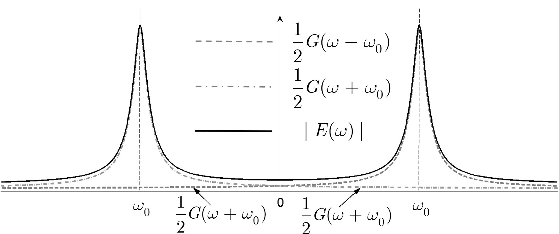
Figure 21: The positive-frequency part of $\mathcal{E}(t,z)$ is given by $\mathcal{E}^{+}(t,z)=\tfrac{1}{2\pi}\int_{0}^{\infty}E(\omega,0)e^{-i\beta(\omega)z}\,e^{i\omega t}d\omega\neq\tfrac{1}{2\pi}\int_{-\infty}^{\infty}\tfrac{1}{2}G(\omega-\omega_{0})e^{-i\beta(\omega)z}\,e^{i\omega t}d\omega\ ,$ because neither $G(\omega-\omega_{0})$ is strictly null on the negative semiaxis, nor $G(\omega+\omega_{0})$ is in the positive semiaxis, as the “tails” marked with arrows in the figure illustrate. In practice, these contributions (greately exagerated in the figure for visualization purposes) are negligible and the narrow-band approximations can be made.

The real electric field $\mathcal{E}$ is finally obtained from the analytical field $\mathcal{\tilde{E}}$ by:

$$\mathcal{E}(t,z) =\mathcal{E}^{+}(t,z)+\mathcal{E}^{-}(t,z)=\mathcal{E}^{+}(t,z)+[\mathcal{E}^{+}(t,z)]^{\ast}=2\operatorname{Re}[\mathcal{E}^{+}(t,z)]$$

$$=\operatorname{Re}[\mathcal{\tilde{E}}(t,z)],$$ (171)

A.5 Spectral width and transform-limited pulses

A.5.1 Uncertainty principle

The propagation of an optical gaussian pulse along a dispersive single-mode fiber is a paradigmatic example of optical pulse propagation that can be found in any textbook on optical communications or general photonics. The well-known result is that the temporal width of the pulse envelope increases with the propagation distance. However, in the frequency domain, the width of the pulse spectrum at the fiber output is found to be exactly the same as at the input. This result often causes confusion as it apparently contradicts the idea that a narrower time signal should have a broader frequency spectrum and vice versa. We will clarify this point here.

The width of an arbitrary pulse-shaped waveform $f(t)$ is usually characterized by its rms width $\sigma_{t},$ given by

$$\sigma_{t}^{2}\equiv\frac{\int_{-\infty}^{\infty}(t-\bar{t})^{2}|f(t)|^{2}dt}{\int_{-\infty}^{\infty}|f(t)|^{2}dt},\qquad\text{with\quad}\bar{t}\equiv\frac{\int_{-\infty}^{\infty}t|f(t)|^{2}dt}{\int_{-\infty}^{\infty}|f(t)|^{2}dt},$$ (172)

$\bar{t}$ being the mean arrival time of the pulse. Note that $\sigma_{t}$ has the same functional form as the standard deviation (the square root of the variance) of a statistical continuous distribution, with $\bar{t}$ playing the role of the the statistical mean. The same definition is used in the frequency domain for the Fourier transforms:

$$\sigma_{\omega}^{2}\equiv\frac{\int_{-\infty}^{\infty}(\omega-\bar{\omega})^{2}|F(\omega)|^{2}d\omega}{\int_{-\infty}^{\infty}|F(\omega)|^{2}d\omega}\qquad\text{with\quad}\bar{\omega}\equiv\frac{\int_{-\infty}^{\infty}\omega|F(\omega)|^{2}d\omega}{\int_{-\infty}^{\infty}|F(\omega)|^{2}d\omega}.$$ (173)

The famous uncertainty principle, first suggested by Heisenberg in the context of Quantum mechanics, follows merely from the mathematical properties of the Fourier transform and is proved with the aid of the Schwartz inequality. It reads

$$\sigma_{t}\,\sigma_{\omega}\geq\dfrac{1}{2}.$$ (174)

However, the equality in (174) holds only for a pure gaussian-shaped Fourier transform pair:

$$f(t)=\exp(-t^{2}/2T^{2})\quad\longleftrightarrow\quad F(\omega)=\sqrt{2\pi}Te^{-\frac{1}{2}T^{2}\omega^{2}}.$$ (175)

In this case,

$$\sigma_{t}^{2}=T^{2}/2,\qquad\sigma_{\omega}^{2}=1/(2T^{2})\qquad\text{and\quad}\sigma_{t}\,\sigma_{\omega}=\frac{1}{2}.$$ (179)

In any case other than a pure gaussian pulse, only ”greater than” applies.

We can never have a pure gaussian baseband pulse in an optical fiber anyway, but, at most, a gaussian pulse-modulated carrier (or “gaussian bandpass pulse”). The electric field and its spectrum at the input of the fiber, $z=0,$ are, in this case,

$$\mathcal{E}_{0}(t) =e^{-t^{2}/2T^{2}}\cos\omega_{0}t$$ (180)

$$E_{0}(\omega) =\frac{1}{2}\sqrt{2\pi}Te^{-\frac{1}{2}T^{2}(\omega-\omega_{0})^{2}}+\frac{1}{2}\sqrt{2\pi}Te^{-\frac{1}{2}T^{2}(\omega+\omega_{0})^{2}}$$

$$\equiv\frac{1}{2}(G(\omega-\omega_{0})+G(\omega+\omega_{0})).$$ (181)

The spectrum is as sketched in Fig. 21. Since (180)–(181) is not a pure gaussian (baseband) Fourier pair, we cannot expect that it will satisfy the equality of relation (174). The calculations yield

$$\sigma_{t}^{2}=\frac{T^{2}}{2}\left(1-\frac{2T^{2}\omega_{0}^{2}}{1+e^{T^{2}\omega_{0}^{2}}}\right)\simeq\frac{T^{2}}{2},\qquad\sigma_{\omega}^{2}=\frac{1}{2T^{2}}+\omega_{0}^{2}\simeq\omega_{0}^{2},$$ (182)

leading to

$$\sigma_{t}\,\sigma_{\omega}\simeq\frac{1}{2}(\omega_{0}T)^{2}>>>\frac{1}{2},$$ (183)

where we have used the narrow-band approximation, $T>>1/\omega_{0}.$ The result (183) indeed complies with (174), but it is not very informative! The problem obviously lies on $\sigma_{\omega}.$ In view of the form of the spectrum, it is not surprising that $\sigma_{\omega}\simeq\omega_{0}$ regardless of the modulating pulse; since $\omega_{0}$ is so much larger than the spectral width of the envelope ($\sim 1/T$), the role of the latter is irrelevant. It is then more profitable to use the analytical signal, i.e., the positive spectrum only. In this case, the pair is

$$e^{-t^{2}/2T^{2}}e^{i\omega_{0}t}\longleftrightarrow e^{-T^{2}(\omega-\omega_{0})^{2}}.$$ (184)

The temporal rms width, which we will call $\tilde{\sigma}_{t},$ is, again,

$$\tilde{\sigma}_{t}^{2}=\frac{T^{2}}{2}.$$ (185)

In the spectral domain, we obtain $\bar{\omega}=\omega_{0}$ and

$$\tilde{\sigma}_{\omega}^{2} =\frac{\int_{-\infty}^{\infty}(\omega-\omega_{0})^{2}e^{-T^{2}(\omega-\omega_{0})^{2}}d\omega}{\int_{-\infty}^{\infty}e^{-T^{2}(\omega-\omega_{0})^{2}}d\omega}$$ (186)

$$=\frac{1}{2T^{2}}\qquad\text{{{\small\{narrow band\}}}.}$$ (187)

Results (185)–(187) appear identical to those for the pure (baseband) gaussian shape, $\sigma_{t}^{2}$ and $\sigma_{\omega}^{2}$ in (179), but we have left the legend “narrow band” as a reminder that the narrow band approximation is implicit in the integrals in (186), which, as explained in the previous subsection, should really be extended between $0$ and $\infty,$ and include the $G(\omega-\omega_{0})$ contribution. As discussed before, the committed error is absolutely negligible. We then obtain

$$\tilde{\sigma}_{t}\,\tilde{\sigma}_{\omega}\simeq\frac{1}{2}.$$ (188)

The product is, strictly speaking, a little bit larger than $1/2$ — a value only reached by a true baseband gaussian pulse —, but the difference is unnoticeable to all practical purposes in the narrow band situation, as one could intuitively expect.

We are finally ready to address the original objective of this subsection. Let us examine what happens to the optical gaussian pulse after propagation along a distance $z.$ We will consider first-order dispersion only and, following the considerations made above for bandpass pulses, we will work with the analytical fields. The following result can be found in any textbook on optical communications:

$$\mathcal{\tilde{E}}_{z}(t) =\exp\left[-\frac{T^{2}(t-z/v_{g})^{2}}{2(T^{4}+\beta_{2}^{2}z^{2})}\right]\times\exp i\left[\omega_{0}t-\beta_{0}z+\frac{\beta_{2}z\,(t-z/v_{g})^{2}}{2(T^{4}+\beta_{2}^{2}z^{2})}\right]$$ (189)

$$\tilde{E}_{z}(\omega) =e^{-\frac{1}{2}T^{2}(\omega-\omega_{0})^{2}}e^{-i\beta(\omega-\omega_{0})z}.$$ (190)

It follows that $\bar{t}=z/v_{g}$ and

$$\tilde{\sigma}_{t}^{2}(z)=\frac{T^{2}}{2}+\frac{z^{2}\beta_{2}^{2}}{2T^{2}}.$$ (191)

Therefore, the temporal width of the pulse does increase with $z$. But the spectral width remains constant:

$$\tilde{\sigma}_{\omega}^{2}(z)=\tilde{\sigma}_{\omega}^{2}(0)=1/(2T^{2}),$$ (192)

since the the dispersive propagation only changes the phase factor of the spectrum, leaving its modulus untouched: $|\exp[-(i\beta(\omega)z)|^{2}=1.$ If follows that

$$\tilde{\sigma}_{t}\,(z)\tilde{\sigma}_{\omega}(z)=\sqrt{\left(\frac{T^{2}}{2}+\frac{z^{2}\beta_{2}^{2}}{2T^{2}}\right)\times\frac{1}{2T^{2}}}=\frac{1}{2}\sqrt{1+\frac{z^{2}\beta_{2}^{2}}{T^{4}}}\geq\frac{1}{2}.$$ (193)

The result (193) does not violate the condition (174); therefore, the uncertainty principle is indeed satisfied.

Note that the product $\tilde{\sigma}_{t}\,(z)\tilde{\sigma}_{\omega}(z),\$apart from being larger than $1/2$, is not constant — it depends on $z.$ Perhaps, we would have expected a result of the type $\tilde{\sigma}_{t}\,(z)\tilde{\sigma}_{\omega}(z)=C$ with $C\geq 1/2$ but fixed. In other words, we would have expected a situation wherein the temporal pulse broadens more and more as it propagates, while its spectrum gets more and more narrow, both effects resulting in constant $\tilde{\sigma}_{t}\,(z)\tilde{\sigma}_{\omega}(z)$ product. But this is not the case. Why? The reader might object, regardless of the mathematical evidence, that both the time signal and the spectrum remain gaussian at any distance $z$, so their Fourier pair should be characterized by the same relation as the pair at $z=0,$ (188). The key here is that the premise is not true — the propagated pulse $\mathcal{\tilde{E}}_{z}(t)$ is not “gaussian” anymore. Even if its envelope is gaussian-shaped, its carrier has now chirp, this is, (dispersion-induced) frequency modulation. Furthermore, the spectrum is not gaussian either; again, only its spectral envelope is, since $\tilde{E}_{z}(\omega)$ now includes a new distortive phase contribution, $\exp[-(i\beta(\omega)z)]$. These characteristics were not present in the original pair (184), so (189) does not qualify as a true gaussian amplitude-modulated carrier, and the result (188) is no longer obtained. Expressed in another way: it is not fair to compare the spectral widths of (180) and (189) because they are different pulses. These remarks are important for understanding the concept of transform-limited pulse, to be addressed in the next subsection.

In contrast to the case considered above, baseband pulses do have a constant product or $\sigma_{t}\,\sigma_{\omega}$, as we have seen with the pure baseband gaussian pulse. Typically, the width of the temporal pulse is proportional to some parameter $T$ and the width of the FT turns out to be proportional to $1/T,$ so that their product maintains a fixed value. Another simple example is the baseband symmetric rectangular pulse of duration $T,$ which FT is a sine cardinal: $\pi_{T}(t)\longleftrightarrow\Pi_{T}(\omega)=\sin(T\omega/2)/(\omega/2).$ In this case, however, the rms measure is useless because $\sigma_{t}=T$ but $\sigma_{\omega}=\infty.$ Indeed $\infty>1/2,$ but this is not certainly a great piece of information, so a more suitable definition for the width should be used. Since both functions are symmetric, the HWHM (half width at half maximum) width can be a good choice. The obtained result is $(\sigma_{t}^{\text{HWHM}})(\sigma_{\omega}^{\text{HWHM}})\simeq(T/2)(2.78/T)=1.39.$

As already said, all these considerations lead us to the concept of “Fourier transform-limited pulse”, which we explain next.

A.5.2 Transform-limited pulses

We have stated that baseband pulses satisfy the Heisenberg relation with a fixed value for the product $\sigma_{t}\,\sigma_{\omega}$ (which depends on the specific pulse shape). This automatically imposes an inverse time-frequency width relation. On the contrary, we have seen two different examples of bandpass pulses, the first, but not the second, having a fixed value of the $\tilde{\sigma}_{t}\,\tilde{\sigma}_{\omega}$ product. What is their difference?

In short, the bandpass pulses with fixed $\tilde{\sigma}_{t}\,\tilde{\sigma}_{\omega}$ product are the so-called “transform-limited” pulses. A transform-limited (or bandwidth-limited) optical pulse is defined as a bandpass pulse “as short as its spectral bandwidth permits”. This statement certainly requires elaboration, but we can explain it with the example of the gaussian pulse. At $z=0$ we have the pulse and its FT given by (184). At $z>0,$ we have (189)–(190). In both cases the frequency span of the FT is the same, but in the second case the pulse is longer. The pulse (184) is transform-limited, but the pulse (189) is not, because, given its temporal width — and this implies looking at its envelope —, it could have had a narrower spectrum. Actually, the pulse (184) is the reference example.

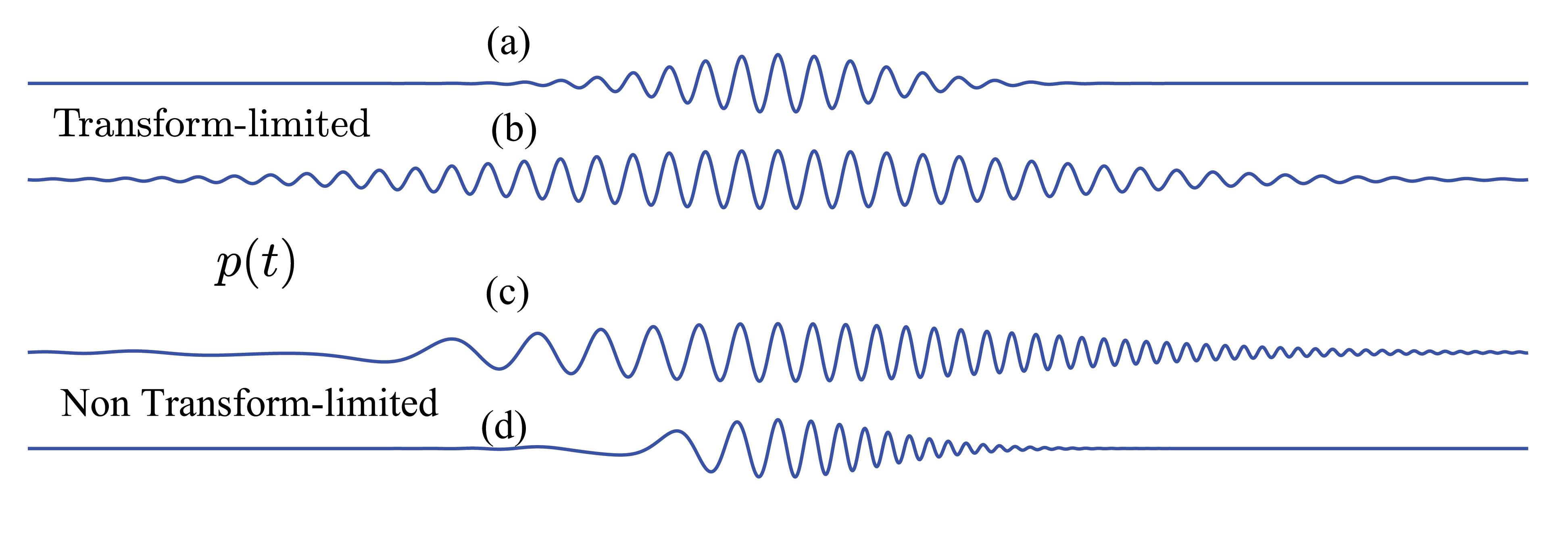
Figure 22: Illustration of the concept of transform-limited pulses. Temporal pulses. See text.

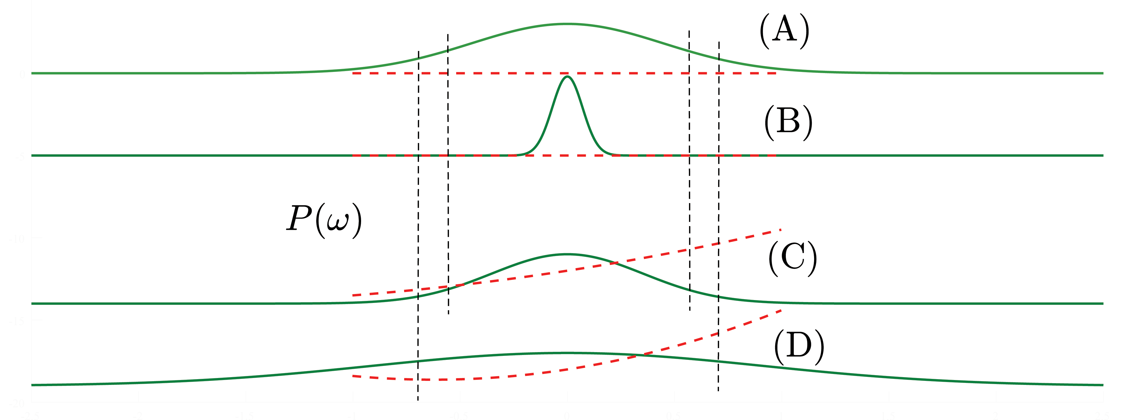
Figure 23: Fourier transforms corresponding to the pulses in Fig. 22. See text.

At this stage we know that the temporal “extra” width of (189) stems from the modulation of its carrier, and this is precisely the idea. Essentially, the transform-limited pulses have a perfectly monochromatic carrier, without any kind of phase/frequency modulation. Such “substructure”, when present, causes the pulse envelope to broaden beyond the minimum duration it could have attained given its given spectral width. This result is summarized in Figs. 22 and 23.

Pulse (a) is an unchirped bandpass gaussian pulse, thus transform-limited. Its spectrum (A) has gaussian modulus and zero phase (dashed line). If the width of the pulse is increased, that of the spectrum decreases, as shown by (b)–(B), and the product $\tilde{\sigma}_{t}\,\tilde{\sigma}_{\omega}$ remains constant (with a value of $1/2$ in this case).

The pair (c)–(C) illustrates the behavior of the pulse (a) after propagating over a distance $z$ along a dispersive optical fiber. The width of the new time pulse (c) is larger than that of pulse (a) —and the carrier becomes chirped—, yet the spectral width of (C) is the same as that of (A). This makes us suspect that the spectrum (C) is “too wide”, and it indeed is: pulse (b), having the same envelope as pulse (c), is spectrally narrower. Consequently, (c) is not transform-limited. (As we have discussed above, the time-chirping of (c) only affects the phase of its spectrum, which is now quadratic, as given by (190): $\beta(\omega-\omega_{0})z\simeq\beta(\omega_{0})z+(\omega-\omega_{0})v_{g}^{-1}x+\frac{1}{2}(\omega-\omega_{0})^{2}\beta_{2}z.$

Finally, (d) is a narrower version of (c), i.e., both pulses have the same expression (189) but (d) has a shorter $T$. As one would expect, (192) predicts a spectrum (D) which is wider than (C), but not in an exactly inverse fashion, with the result that $\tilde{\sigma}_{t}\,\tilde{\sigma}_{\omega}\neq\,$constant, as (193) evidences. Note that, as sketched in the figure, the spectrum (D) is necessarily broader than (A) as well, because, while the corresponding time envelopes of (a) and (d) being identical, (d) is chirped and (a) is not. Naturally, all these considerations are not exclusive for gaussian-shaped pulses; they apply to any waveform.

References

- [1] N. W. Ashcroft and N. D. Mermin, Solid state physics. New York: Holt, Rinehart and Winston, 1976.
- [2] K. Cho, Reconstruction of macroscopic Maxwell equations a single susceptibility theory. Heidelberg; New York: Springer, 2010.
- [3] S. L. Chuang, Physics of Optoelectronic Devices. Wiley, 1995.
- [4] E. D. Palik, Handbook of Optical Constants of Solids. Academic Press, 1998.
- [5] M. Fox, Optical Properties of Solids, 2nd ed. Oxford ; New York: OUP Oxford, 2010.
- [6] M. Bass, E. W. V. Stryland, D. R. Williams, and W. L. Wolfe, Handbook of Optics Volume II Devices, Measurements, and Properties 2nd edition, 1995.
- [7] F. d. Coulon, Signal theory and processing. Dedham, MA : Artech House, 1986.
- [8] L. D. Landau, E. M. Lifshitz, V. B. Berestetskii, and L. P. Pitaevskii, Electrodynamics of continuous media. Oxford: Butterworth-Heinemann, 1995.
- [9] D. L. Mills, Nonlinear Optics: Basic Concepts, 2nd ed. Berlin ; New York: Springer, 1998.
- [10] P. Chamorro-Posada and F. J. Fraile-Pelaez, “Superluminal propagation in resonant dissipative media,” Optics Communications, vol. 282, no. 6, pp. 1095–1098, Mar. 2009.
- [11] G. M. Gehring, A. Schweinsberg, C. Barsi, N. Kostinski, and R. W. Boyd, “Observation of backward pulse propagation through a medium with a negative group velocity,” Science, vol. 312, no. 5775, pp. 895–897, 2006.
- [12] P. Chamorro-Posada and F. J. Fraile-Pelaez, “Fast and slow light in zigzag microring resonator chains,” Optics Letters, vol. 34, no. 5, p. 626, Feb. 2009.
- [13] I. Cestier, V. Eckhouse, G. Eisenstein, S. Combrié, P. Colman, and A. D. Rossi, “Resonance enhanced large third order nonlinear optical response in slow light GaInP photonic-crystal waveguides,” Optics Express, vol. 18, no. 6, pp. 5746–5753, Mar. 2010.
- [14] R. W. Boyd, D. J. Gauthier, and A. L. Gaeta, “Applications of slow light in telecommunications,” Optics and Photonics News, vol. 17, no. 4, pp. 18–23, Apr. 2006.
- [15] A. Yariv and P. Yeh, Photonics: optical electronics in modern communications, 6th ed. Oxford: Oxford University Press, 2007.
- [16] A. E. Siegman, Lasers. Mill Valley, California: University Science Books, 1990.