Proper TMD factorization for quarkonia production: $pp\to\eta_{c,b}$ as a study case

Abstract

Quarkonia production in different high-energy processes has recently been proposed in order to probe gluon transverse-momentum-dependent parton distribution and fragmentation functions (TMDs in general). However, no proper factorization theorems have been derived for the discussed processes, but rather just ansatzs, whose main assumption is the factorization of the two soft mechanisms present in the process: soft-gluon radiation and the formation of the bound state. In this paper it is pointed out that, at low transverse momentum, these mechanisms are entangled and thus encoded in a new kind of non-perturbative hadronic quantities beyond the TMDs: the TMD shape functions. This is illustrated by deriving the factorization theorem for the process $pp\to\eta_{c,b}$ at low transverse momentum.

I Motivation

Gluons, together with quarks, are the fundamental constituents of nucleons. They generate almost all their mass and carry about half of their momentum. However, their three-dimensional (3D) structure is still unknown, as well as their contribution to the nucleon spin. The 3D structure of hadrons in momentum space is parametrized by the so-called Transverse-Momentum-Dependent Parton Distribution/Fragmentation functions (TMDPDFs/TMDFFs, TMDs in general) Angeles-Martinez:2015sea . These are the 3D generalization of the one-dimensional PDFs and FFs, where a dependence on the transverse momentum of the partons is also allowed. They include as well the correlations between this transverse momentum and the spins of the considered parton and its parent hadron.

Constraining gluon TMDs is a crucial step in our understanding of nucleon 3D structure, and with that also our understanding of confinement in QCD and the structure of ordinary matter in general. In fact, the study of gluon TMDs in particular, and the gluon content of the nucleons in general, is one of the main motivations that is pushing forward the design of the Electron-Ion Collider in the US Accardi:2012qut and fixed-target experiments at the LHC at CERN Hadjidakis:2018ifr ; Kikola:2017hnp ; Trzeciak:2017csa ; Brodsky:2012vg .

In the last years a huge step forward has been made in the quark TMDs sector, obtaining their proper definition and properties, and their connection with observable cross-sections in terms of robust factorization theorems GarciaEchevarria:2011rb ; Echevarria:2012pw ; Echevarria:2012js ; Echevarria:2014rua ; Collins:2011zzd . This, together with new higher-order perturbative calculations (see e.g. Gutierrez-Reyes:2019rug ; Gutierrez-Reyes:2018iod ; Echevarria:2016scs ; Echevarria:2015byo ; Echevarria:2015usa ), has allowed the phenomenological analyses to enter a new precision stage (see e.g. DAlesio:2014mrz ; Echevarria:2014xaa ; Bacchetta:2015ora ; Bacchetta:2017gcc ; Anselmino:2016uie ; Scimemi:2017etj ; Bertone:2019nxa ). However, for gluons the situation is very different. Even if their proper definition is currently known Echevarria:2015uaa , the processes where they can be probed are less clean compared to the ones which are used to access quark TMDs.

All and all, quarkonium production seems the most promising way to probe gluon TMDs. Indeed, there has been a growing interest lately, with numerous proposals based on tree-level ansatzs for TMD factorization for quarkonium production Godbole:2012bx ; Boer:2012bt ; Godbole:2013bca ; Godbole:2014tha ; Zhang:2014vmh ; Zhang:2015yba ; Mukherjee:2015smo ; Mukherjee:2016qxa ; Mukherjee:2016cjw ; Boer:2016bfj ; Lansberg:2017tlc ; Godbole:2017syo ; DAlesio:2017rzj ; Rajesh:2018qks ; Bacchetta:2018ivt ; Lansberg:2017dzg ; Kishore:2018ugo ; Scarpa:2019fol and even several next-to-leading-order (NLO) calculations Sun:2012vc ; Ma:2012hh ; Ma:2014oha ; Ma:2015vpt .

The caveat shared by all these attempts, however, is that all of them assume the decoupling of the two soft mechanisms present in the processes: the soft physics underlying the formation of the quarkonium bound state and the soft gluon resummation. Indeed, these two soft phenomena cannot be factorized when their relevant scales are comparable, i.e. when $q_{T}\sim m_{Q}v$, being $q_{T}$ the measured transverse momentum and $m_{Q}v$ the typical momentum of a heavy quark of mass $m_{Q}$ and velocity $v$ inside the quarkonium state. For $b\bar{b}$ states one typically has $v^{2}\sim 0.1$, while for $c\bar{c}$ one has $v^{2}\sim 0.3$, so then $m_{b}v\sim 1.3~{}\rm GeV$ and $m_{c}v\sim 0.7~{}\rm GeV$. Roughly speaking, when the transverse momentum is in the non-perturbative region around and below $\Lambda_{\rm QCD}$, then the factorization ansatz made in all previous analyses is not accurate. And it is precisely this region which is claimed to be sensitive to gluon TMDs and where they can potentially be probed.

In this paper the process $pp\to\eta_{c,b}+X$ is considered as an example of quarkonium production process, and the factorization theorem at low transverse momentum is derived. It turns out that the cross-section is not given only in terms of gluon TMDs, but there is an additional new non-perturbative hadronic quantity which encodes the two mentioned soft processes together: the TMD shape function. Using the newly derived factorization theorem, the hard part of the process is obtained at one-loop, which is an essential ingredient for future phenomenological analyses since it allows the resummation of large logarithms at higher logarithmic orders. Moreover, the obtention of a hard factor free from infrared divergences represents a non-trivial consistency check of the newly derived factorization theorem.

II Factorization theorem for $pp\to\eta_{c,b}+X$ at low $q_{T}$

The differential cross section for $\eta_{Q}$ ($Q=c,b$) hadro-production is given by

$$d\sigma=\frac{1}{2s}\frac{d^{3}q}{(2\pi)^{3}2E_{q}}\int d^{4}\xi\,e^{-iq\cdot\xi}\,\sum_{X}\left<PS_{A},\bar{P}S_{B}\right|{\mathcal{O}}^{\dagger}(\xi)\left|X\eta_{Q}\right>\,\left<\eta_{Q}X\right|{\mathcal{O}}(0)\left|PS_{A},\bar{P}S_{B}\right>\,,$$ (1)

where $s=(P+\bar{P})^{2}$. The effective operator which mediates this process within an effective theory which combines both soft-collinear effective theory (SCET) Bauer:2000ew ; Bauer:2000yr ; Bauer:2001ct ; Bauer:2001yt ; Bauer:2002nz ; Beneke:2002ph and non relativistic QCD (NRQCD) Bodwin:1994jh degrees of freedom can be written as 

$${\cal O}(\xi)=-2q^{2}\sum_{n}C_{H}^{(n)}(-q^{2};\mu^{2})\,\Big{[}\psi^{\dagger}(\xi)\,\Gamma_{\mu\nu}^{(n)}K_{aa^{\prime}}^{[1,8]}\,\chi(\xi)\Big{]}\,\Big{[}B_{{\bar{n}}\perp}^{\mu,b}(\xi)\,{\mathcal{Y}}_{\bar{n}}^{\dagger ba}(\xi)\,{\mathcal{Y}}_{n}^{a^{\prime}c}(\xi)\,B_{n\perp}^{\nu,c}(\xi)\Big{]}\,,$$ (2)

where the sum runs over the different states $n$ which can contribute to the process. In the usual spectroscopic notation, $n$ stands for ${}^{2S+1}L_{J}^{[i]}$, with $S$ the spin, $L$ the angular momentum and $J$ the total angular momentum, and $i=1(8)$ for singlet (octet). $C_{H}^{(n)}$ are the spin-independent matching coefficients for each state $n$, which integrate out the hard scale of the process, $q^{2}=M^{2}$. $a,a^{\prime}b,c$ are the gauge group indexes, while $\Gamma^{(n)}_{\mu\nu}$ is a matrix which encodes the Lorentz structure of the partonic process for the creation of the state $n$. $K_{aa^{\prime}}$ is a color matrix, with $K_{aa^{\prime}}^{[1]}=\delta_{aa^{\prime}}$ for color-singlet states and $K_{aa^{\prime}}^{[8]}=t^{A}_{aa^{\prime}}$ for color-octet states. $\chi$ and $\psi$ are the spinors describing the $Q\bar{Q}$ state. The $B_{n({\bar{n}})}^{\perp\mu}$ operators, which stand for gauge invariant gluon fields, are given by

$$B_{n\perp}^{\mu}=B_{n\perp}^{\mu,a}t^{a}=\frac{1}{g}[W_{n}^{\dagger}iD_{n}^{\perp\mu}W_{n}]=\frac{1}{{\bar{n}}\!\cdot\!{\mathcal{P}}}i{\bar{n}}_{\alpha}g^{\mu}_{\perp\beta}W_{n}^{\dagger}F_{n}^{\alpha\beta}W_{n}\frac{1}{{\bar{n}}\!\cdot\!{\mathcal{P}}}i{\bar{n}}_{\alpha}g^{\mu}_{\perp\beta}t^{a}({\mathcal{W}}_{n}^{\dagger})^{ab}F_{n}^{\alpha\beta,b}\,.$$ (3)

The collinear and soft Wilson lines are the path-ordered exponentials

$$W_{n}(\xi) =P\exp\left[ig\int_{-\infty}^{0}ds\,{\bar{n}}\!\cdot\!A_{n}^{a}(\xi+{\bar{n}}s)t^{a}\right]\,,$$

$$Y_{n}(\xi) =P\exp\left[ig\int_{-\infty}^{0}ds\,n\!\cdot\!A_{s}^{a}(\xi+ns)t^{a}\right]\,.$$ (4)

Wilson lines with calligraphic typography are in the adjoint representation, i.e., the color generators are given by $(t^{a})^{bc}=-if^{abc}$. In order to guarantee gauge invariance among regular and singular gauges, transverse gauge links need to be added (as described in Idilbi:2010im ; GarciaEchevarria:2011md ).

In the case of $\eta_{Q}$ production, NRQCD formalism dictates that the operator for the state ${}^{1}S_{0}^{[1]}$ is the leading one in the power counting in the velocity $v$ Bodwin:1994jh . Thus from now on we will consider only that contribution. Moreover, the production of color-octet states will potentially spoil TMD factorization due to the presence of uncanceled Glauber gluons Collins:2007nk ; Collins:2007jp ; Rogers:2010dm . The Lorentz structure $\Gamma_{\mu\nu}^{{}^{1}S_{0}}$ is fixed by requiring the effective operator to give the same tree-level amplitude as in full QCD for the production of a pseudoscalar $\eta_{Q}$ in the configuration ${}^{1}S_{0}^{[1]}$:

$$\Gamma_{\mu\nu}^{{}^{1}S_{0}} =\frac{i\pi\alpha_{s}2\sqrt{2}}{N_{c}\sqrt{M^{5}}}\epsilon_{\perp\mu\nu}\,,$$ (5)

where $\epsilon_{\perp}^{\mu\nu}=\epsilon^{\alpha\beta\mu\nu}n^{\alpha}{\bar{n}}^{\beta}/(n\cdot{\bar{n}})$, with $\epsilon_{\perp}^{12}=1$.

The effective Lagrangian for this process is given by the combination of both SCET and NRQCD effective Lagrangians. This means that (anti)collinear modes are decoupled from soft and ultrasoft modes, while the latter are coupled among them (through the NRQCD Lagrangian). One can thus decompose the final state as the following product of states:

$$\left|X\eta_{Q}\right> =\left|X_{n}\right>\otimes\left|X_{\bar{n}}\right>\otimes\left|X_{s}\eta_{Q}\right>\,,$$ (6)

where $X_{n,{\bar{n}},s}$ are the collinear, anticollinear and soft modes of the unobserved final states. Notice that the state $\eta_{Q}$ cannot be decoupled from $X_{s}$. A similar decomposition applies to the initial state, considering proton A to be collinear and proton B anticollinear:

$$\left|PS_{A},\bar{P}S_{B}\right>=\left|PS_{A}\right>\otimes\left|\bar{P}S_{B}\right>\,.$$ (7)

Using the decompositions in modes (6) and (7) the cross section is written as

$$d\sigma=\frac{1}{2s}\frac{d^{3}q}{(2\pi)^{3}2E_{q}}\,4M^{4}\,H(M^{2},\mu^{2})\,\Gamma^{*}_{\rho\sigma}\Gamma_{\mu\nu}\int d^{4}\xi\ e^{-iq\xi}$$

$$\quad\times\sum_{X_{n}}\,\left<PS_{A}\right|B_{n\perp}^{\sigma,c^{\prime}}(\xi)\left|X_{n}\right>\left<X_{n}\right|B_{n\perp}^{\nu,c}(0)\left|PS_{A}\right>\,\sum_{X_{{\bar{n}}}}\,\left<\bar{P}S_{B}\right|B_{\bar{n}\perp}^{\rho,b^{\prime}}(\xi)\left|X_{{\bar{n}}}\right>\left<X_{{\bar{n}}}\right|B_{{\bar{n}}\perp}^{\mu,b}(0)\left|\bar{P}S_{B}\right>$$

$$\quad\times\sum_{X_{s}}\left<0\right|\Big{[}{\mathcal{Y}}_{n}^{\dagger c^{\prime}a^{\prime}}{\mathcal{Y}}_{\bar{n}}^{a^{\prime}b^{\prime}}\chi^{\dagger}\psi\Big{]}(\xi)\left|X_{s}\eta_{Q}\right>\,\left<\eta_{Q}X_{s}\right|\Big{[}{\mathcal{Y}}_{\bar{n}}^{\dagger ba}{\mathcal{Y}}_{n}^{ac}\psi^{\dagger}\chi\Big{]}(0)\left|0\right>\,,$$ (8)

where $H(M^{2},\mu^{2})=|C_{H}(-q^{2};\mu^{2})|^{2}$. The Lorentz structure $\Gamma_{\mu\nu}\equiv\Gamma_{\mu\nu}^{{}^{1}S_{0}}$ is kept for simplicity. This result needs to be Taylor expanded in order to extract the leading contribution with a homogenous power counting. The produced quarkonium is hard with momentum $q\sim M(1,1,\lambda)$, where $\lambda$ is a small parameter parametrizing the relative strength of the momentum components of different modes, $\lambda\sim q_{T}/M$. In the exponent $e^{-iq\xi}$ in (1) one then has $\xi\sim M(1,1,1/\lambda)$. In addition, the scalings of the derivatives of the collinear, anticollinear and soft terms are the same as their respective momentum scalings. Given this, the obtained leading term in the Taylor expansion of the cross section is

$$d\sigma=\frac{1}{2s}\frac{d^{3}q}{(2\pi)^{3}2E_{q}}\,\frac{4M^{4}\,H(M^{2},\mu^{2})}{(N_{c}^{2}-1)^{2}}\,\Gamma^{*}_{\rho\sigma}\Gamma_{\mu\nu}\int d^{4}\xi\ e^{-iq\xi}$$

$$\quad\times\left<PS_{A}\right|B_{n\perp}^{\sigma,c}(\xi^{-},\xi_{\perp})\,B_{n\perp}^{\nu,c}(0)\left|PS_{A}\right>\,\left<\bar{P}S_{B}\right|B_{{\bar{n}}\perp}^{\rho,b}(\xi^{+},\xi_{\perp})\,B_{{\bar{n}}\perp}^{\mu,b}(0)\left|\bar{P}S_{B}\right>\,$$

$$\quad\times\left<0\right|\Big{[}{\mathcal{Y}}_{n}^{\dagger ca^{\prime}}{\mathcal{Y}}_{\bar{n}}^{a^{\prime}b}\chi^{\dagger}\psi\Big{]}(\xi_{\perp})\,a_{\eta_{Q}}^{\dagger}a_{\eta_{Q}}\,\Big{[}{\mathcal{Y}}_{\bar{n}}^{\dagger ba}{\mathcal{Y}}_{n}^{ac}\psi^{\dagger}\chi\Big{]}(0)\left|0\right>+{\mathcal{O}}(\lambda)\,,$$ (9)

where we have also used the fact that (anti)collinear matrix elements are diagonal in color, and the completeness relations

$$\sum_{X_{n}}\left|X_{n}\right>\left<X_{n}\right|=1\,,\quad\sum_{X_{\bar{n}}}\left|X_{\bar{n}}\right>\left<X_{\bar{n}}\right|=1\,,$$

$$\sum_{X_{s}}\left|X_{s}\eta_{Q}\right>\left<X_{s}\eta_{Q}\right|=a_{\eta_{Q}}^{\dagger}\sum_{X_{s}}\left|X_{s}\right>\left<X_{s}\right|a_{\eta_{Q}}=a_{\eta_{Q}}^{\dagger}a_{\eta_{Q}}\,.$$ (10)

Performing standard algebraic manipulations and dropping the suppressed terms, the cross-section can be written as:

$$\frac{d\sigma}{dyd^{2}q_{\perp}}=\frac{4M^{4}\,H(M^{2},\mu^{2})}{2sM^{2}(N_{c}^{2}-1)}\,\Gamma^{*}_{\rho\sigma}\Gamma_{\mu\nu}(2\pi)\int d^{2}\mbox{\boldmath$k$}_{n\perp}d^{2}\mbox{\boldmath$k$}_{{\bar{n}}\perp}d^{2}\mbox{\boldmath$k$}_{s\perp}\,\delta^{(2)}\left(\mbox{\boldmath$q$}_{\perp}-\mbox{\boldmath$k$}_{n\perp}-\mbox{\boldmath$k$}_{{\bar{n}}\perp}-\mbox{\boldmath$k$}_{s\perp}\right)$$

$$\quad\times J_{n}^{(0)\sigma\nu}(x_{A},\mbox{\boldmath$k$}_{n\perp},S_{A};\mu;\delta_{n})\,J_{{\bar{n}}}^{(0)\rho\mu}(x_{B},\mbox{\boldmath$k$}_{{\bar{n}}\perp},S_{B};\mu;\delta_{\bar{n}})\,S_{\eta_{Q}}^{(0)}\!\Big{[}{}^{1}S_{0}^{[1]}\Big{]}(\mbox{\boldmath$k$}_{s\perp};\mu;\delta_{n},\delta_{\bar{n}})\,,$$ (11)

where $x_{A,B}=\sqrt{\tau}\,e^{\pm y}$, $\tau=(M^{2}+q_{T}^{2})/s$ and $y$ is the rapidity of the produced $\eta_{Q}$. The pure collinear matrix elements $J^{(0)}_{n({\bar{n}})}$ and the bare TMD shape function $S_{\mathcal{Q}}^{(0)}$ (TMDShF from now on) are defined as

$$J_{n}^{(0)\mu\nu}=\frac{x_{A}P^{+}}{2}\int\frac{d\xi^{-}d^{2}\mbox{\boldmath$\xi$}_{\perp}}{(2\pi)^{3}}\,e^{-i\left(\frac{1}{2}x_{A}\xi^{-}P^{+}-\mbox{\boldmath${\scriptstyle\xi}$}_{\perp}\!\cdot\!\mbox{\boldmath${\scriptstyle k}$}_{n\perp}\right)}\,\left<PS_{A}\right|B_{n\perp}^{\mu,a}(\xi^{-},\mbox{\boldmath$\xi$}_{\perp})\,B_{n\perp}^{\nu,a}(0)\left|PS_{A}\right>\,,$$

$$J_{\bar{n}}^{(0)\mu\nu}=\frac{x_{B}\bar{P}^{-}}{2}\int\frac{d\xi^{+}d^{2}\mbox{\boldmath$\xi$}_{\perp}}{(2\pi)^{3}}\,e^{-i\left(\frac{1}{2}x_{B}\xi^{+}\bar{P}^{-}-\mbox{\boldmath${\scriptstyle\xi}$}_{\perp}\!\cdot\!\mbox{\boldmath${\scriptstyle k}$}_{{\bar{n}}\perp}\right)}\,\left<\bar{P}S_{B}\right|B_{{\bar{n}}\perp}^{\mu,a}(\xi^{+},\mbox{\boldmath$\xi$}_{\perp})\,B_{{\bar{n}}\perp}^{\nu,a}(0)\left|\bar{P}S_{B}\right>\,,$$

$$S_{\eta_{Q}}^{(0)}\!\Big{[}{}^{1}S_{0}^{[1]}\Big{]}=\frac{1}{N_{c}^{2}-1}\,\int\frac{d^{2}\mbox{\boldmath$\xi$}_{\perp}}{(2\pi)^{2}}\,e^{i\mbox{\boldmath${\scriptstyle\xi}$}_{\perp}\!\cdot\!\mbox{\boldmath${\scriptstyle k}$}_{s\perp}}\,\left<0\right|\Big{[}{\mathcal{Y}}_{n}^{\dagger ab}{\mathcal{Y}}_{\bar{n}}^{bc}\chi^{\dagger}\psi\Big{]}(\mbox{\boldmath$\xi$}_{\perp})\,a_{\eta_{Q}}^{\dagger}a_{\eta_{Q}}\,\Big{[}{\mathcal{Y}}_{\bar{n}}^{\dagger cd}{\mathcal{Y}}_{n}^{da}\psi^{\dagger}\chi\Big{]}(0)\left|0\right>\,.$$ (12)

Notice that the spurious contribution of the soft momentum modes in the naively calculated collinear matrix elements, denoted $J_{n({\bar{n}})}$ (the so-called “zero-bin” in the SCET nomenclature), should be subtracted, in order to avoid their double counting.

Both the collinear matrix elements and the bare TMDShF in (II) have been written with a dependence on $\delta_{n({\bar{n}})}$, which stand for generic rapidity regulators. These divergences cancel in the full combination of the three matrix elements. However a different soft function needs to be invoked in order to properly define the gluon TMDs:

$$S=\frac{1}{N_{c}^{2}-1}\,\int\frac{d^{2}\mbox{\boldmath$\xi$}_{\perp}}{(2\pi)^{2}}\,e^{i\mbox{\boldmath${\scriptstyle\xi}$}_{\perp}\!\cdot\!\mbox{\boldmath${\scriptstyle k}$}_{s\perp}}\,\left<0\right|\Big{[}{\mathcal{Y}}_{n}^{\dagger ab}{\mathcal{Y}}_{\bar{n}}^{bc}\Big{]}(\mbox{\boldmath$\xi$}_{\perp})\,\Big{[}{\mathcal{Y}}_{\bar{n}}^{\dagger cd}{\mathcal{Y}}_{n}^{da}\Big{]}(0)\left|0\right>\,.$$ (13)

This soft function can be split in rapidity space to all orders in perturbation theory as Echevarria:2015byo

$$\tilde{S}(\xi_{T};\mu;\delta_{n},\delta_{\bar{n}}) =\tilde{S}_{-}\left(\xi_{T};\mu;\delta_{n}\right)\tilde{S}_{+}\left(\xi_{T};\mu;\delta_{\bar{n}}\right)\,.$$ (14)

With these pieces, the gluon TMDPDFs are defined as Echevarria:2015uaa

$${\tilde{G}}_{g/A}^{\mu\nu}(x_{A},\mbox{\boldmath$\xi$}_{\perp},S_{A};\zeta_{A},\mu) =\tilde{J}_{n}^{(0)\mu\nu}(x_{A},\mbox{\boldmath$\xi_{\perp}$},S_{A};\mu;\delta_{n})\,\tilde{S}_{-}(\xi_{T};\mu;\delta_{n})\,,$$

$${\tilde{G}}_{g/B}^{\mu\nu}(x_{B},\mbox{\boldmath$\xi$}_{\perp},S_{B};\zeta_{B},\mu) =\tilde{J}_{{\bar{n}}}^{(0)\mu\nu}(x_{B},\mbox{\boldmath$\xi_{\perp}$},S_{B};\mu;\delta_{\bar{n}})\,\tilde{S}_{+}(\xi_{T};\mu;\delta_{\bar{n}})\,,$$ (15)

where $\zeta_{A,B}$ are auxiliary energy scales which arise when the rapidity divergences are cancelled in each TMD, and the twiddle labels the functions in coordinate space. The chosen rapidity regulator is arbitrary, however the auxiliary energy scales $\zeta_{A}$ and $\zeta_{B}$ in the TMDs are bound together by $\zeta_{A}\zeta_{B}=q^{4}=M^{4}$. We emphasize that gluon TMDs so defined are free from rapidity divergences, i.e., they have well-behaved evolution properties and can be extracted from experimental data.

Given the definitions in (II), the factorized cross-section for proton-proton collisions at low $q_{T}$ is finally written as

$$\frac{d\sigma}{dy\,d^{2}q_{\perp}}=\frac{4M^{4}\,H(M^{2},\mu^{2})}{2sM^{2}(N_{c}^{2}-1)}\,\Gamma^{*}_{\rho\sigma}\Gamma_{\mu\nu}(2\pi)\int d^{2}\mbox{\boldmath$k$}_{n\perp}d^{2}\mbox{\boldmath$k$}_{{\bar{n}}\perp}d^{2}\mbox{\boldmath$k$}_{s\perp}\,\delta^{(2)}\left(\mbox{\boldmath$q$}_{\perp}-\mbox{\boldmath$k$}_{n\perp}-\mbox{\boldmath$k$}_{{\bar{n}}\perp}-\mbox{\boldmath$k$}_{s\perp}\right)$$

$$\quad\times G_{g/A}^{\sigma\nu}(x_{A},\mbox{\boldmath$k$}_{n\perp},S_{A};\zeta_{A},\mu)\,G_{g/B}^{\rho\mu}(x_{B},\mbox{\boldmath$k$}_{{\bar{n}}\perp},S_{B};\zeta_{B},\mu)\,S_{\eta_{Q}}\!\Big{[}{}^{1}S_{0}^{[1]}\Big{]}(\mbox{\boldmath$k$}_{s\perp};\mu)\,,$$ (16)

where we have defined, for convenience, the TMDShF free from rapidity divergences as

$${\tilde{S}}_{\eta_{Q}}\!\Big{[}{}^{1}S_{0}^{[1]}\Big{]}(\xi_{T};\mu) =\frac{\tilde{S}_{\eta_{Q}}^{(0)}\!\Big{[}{}^{1}S_{0}^{[1]}\Big{]}(\xi_{T};\mu)}{\tilde{S}(\xi_{T};\mu)}\,.$$ (17)

Given that there are no other vectors available, the TMDShF, as the soft function, depends on the modulus $\xi_{T}$.

The factorization theorem in (II) is the main result of this letter. It contains 3 non-perturbative hadronic quantities at low transverse momentum: two gluon TMDPDFs, and the newly defined TMDShF. Thus, the phenomenological extraction of gluon TMDs from quarkonium production processes is still possible, i.e., a robust factorization theorem can potentially be obtained like in this particular case of $\eta_{c,b}$ hadro-production. However one also needs to model and extract the involved TMDShFs for the relevant angular/color configurations.

Notice that, while the factorized cross-section in (II) contains all the (un)polarized gluon TMDs, the TMDShF ${\tilde{S}}_{\eta_{Q}}\!\Big{[}{}^{1}S_{0}^{[1]}\Big{]}$ is spin independent. In particular, if unpolarized proton collisions are considered, which is relevant e.g. for the LHC, one can parametrize the gluon TMD $G_{g/A}^{\mu\nu}$ in momentum space as

$$G_{g/A}^{\mu\nu}(x_{A},\mbox{\boldmath$k$}_{\perp},S_{A};\zeta_{A},\mu)\equiv\frac{1}{2}\bigg{[}-g_{\perp}^{\mu\nu}f_{1}^{g}(x_{A},k_{T}^{2};\zeta_{A},\mu)+\frac{k_{T}^{\mu\nu}}{M_{p}^{2}}h_{1}^{\perp g}(x_{A},k_{T}^{2};\zeta_{A},\mu)\bigg{]}\ ,$$ (18)

where $M_{p}$ is the mass of the proton and $k_{T}^{\mu\nu}$ is a symmetric traceless tensor of rank 2 Boer:2016xqr :

$$k_{T}^{\mu\rho} =k_{\perp}^{\mu}k_{\perp}^{\rho}+\frac{1}{2}\mbox{\boldmath$k$}_{\perp}^{2}g_{\perp}^{\mu\rho}\,.$$ (19)

The function $f_{1}^{g}$ is the TMDPDF for unpolarized gluons in an unpolarized proton, while $h_{1}^{\perp g}$ parametrizes linearly polarized gluons inside an unpolarized proton. The parametrization in position space reads

$${\tilde{G}}_{g/A}^{\mu\nu}(x_{A},\mbox{\boldmath$b$}_{\perp},S_{A};\zeta_{A},\mu)\equiv\frac{1}{2}\bigg{[}-g_{\perp}^{\mu\nu}\tilde{f}_{1}^{g}(x_{A},b_{T}^{2};\zeta_{A},\mu)-\frac{M_{p}^{2}}{2}b_{T}^{\mu\nu}\tilde{h}_{1}^{\perp g(2)}(x_{A},b_{T}^{2};\zeta_{A},\mu)\bigg{]}\,,$$ (20)

where the Fourier transform of the functions and their moments follow the conventions in Boer:2016xqr .

Inserting the decomposition (18) in (II), one obtains the factorized cross section for collisions of unpolarized protons:

$$\frac{d\sigma}{dyd^{2}q_{\perp}}=\sigma_{0}(\mu)H(M^{2},\mu^{2})\,\Big{[}{\mathcal{C}}[f_{1}^{g}f_{1}^{g}S_{\mathcal{Q}}]-{\mathcal{C}}[w_{UU}h_{1}^{\perp g}h_{1}^{\perp g}S_{Q\bar{Q}}]\Big{]}\,,$$ (21)

where $S_{\cal Q}$ stands for $S_{\eta_{Q}}\!\Big{[}{}^{1}S_{0}^{[1]}\Big{]}$ and the Born-level cross-section is

$$\sigma_{0} =\frac{(4\pi\alpha_{s})^{2}\pi}{N_{c}^{2}(N_{c}^{2}-1)sM^{3}}\,.$$ (22)

The convolutions ${\mathcal{C}}$ are defined in general as:

$$\mathcal{C}[w\,f\,f\,S_{\mathcal{Q}}]\equiv\int d^{2}\mbox{\boldmath$p$}_{\perp a}\,d^{2}\mbox{\boldmath$p$}_{\perp b}\,d^{2}\mbox{\boldmath$k$}_{\perp}\,\delta^{2}(\mbox{\boldmath$p$}_{\perp a}+\mbox{\boldmath$p$}_{\perp b}+\mbox{\boldmath$k$}_{\perp}-\mbox{\boldmath$q$}_{\perp})$$

$$\quad\times w(p_{\perp a},p_{\perp b})\,f(x_{A},\mbox{\boldmath$p$}_{Ta}^{2};\zeta_{A},\mu)\,f(x_{B},\mbox{\boldmath$p$}_{Tb}^{2};\zeta_{B},\mu)\,S_{\mathcal{Q}}(k_{T}^{2};\mu)\,,$$ (23)

and the transverse momentum weight $w_{UU}$ for the contribution of linearly polarized gluon TMDs is

$$w_{UU}=\frac{p_{\perp a}^{\mu\nu}\ p_{\perp b\,\mu\nu}}{2M_{p}^{4}}\,.$$ (24)

Given this, the two Fourier transforms are

$${\mathcal{C}}[f_{1}^{g}f_{1}^{g}S_{\mathcal{Q}}]=\int\frac{d^{2}\mbox{\boldmath$b$}_{T}}{(2\pi)^{2}}\ e^{i\mbox{\boldmath${\scriptstyle b}$}_{T}\cdot\mbox{\boldmath${\scriptstyle q}$}_{T}}\,\tilde{f}_{1}^{g}(x_{A},b_{T}^{2};\zeta_{A},\mu)\,\tilde{f}_{1}^{g}(x_{B},b_{T}^{2};\zeta_{B},\mu)\,S_{\mathcal{Q}}(b_{T}^{2};\mu)$$

$$=\frac{1}{2\pi}\int_{0}^{+\infty}db_{T}b_{T}J_{0}(b_{T}q_{T})\,\tilde{f}_{1}^{g}(x_{A},b_{T}^{2};\zeta_{A},\mu)\,\tilde{f}_{1}^{g}(x_{B},b_{T}^{2};\zeta_{B},\mu)\,S_{\mathcal{Q}}(b_{T}^{2};\mu)\,,$$ (25)

and

$${\mathcal{C}}[w_{UU}h_{1}^{\perp g}h_{1}^{\perp g}S_{\mathcal{Q}}]=\frac{M_{p}^{4}}{16}\int\frac{d^{2}\mbox{\boldmath$b$}_{T}}{(2\pi)^{2}}\ e^{i\mbox{\boldmath${\scriptstyle b}$}_{T}\cdot\mbox{\boldmath${\scriptstyle q}$}_{T}}\,\mbox{\boldmath$b$}_{T}^{4}\,\tilde{h}_{1}^{\perp g(2)}(x_{A},b_{T}^{2};\zeta_{A},\mu)\,\tilde{h}_{1}^{\perp g(2)}(x_{B},b_{T}^{2};\zeta_{B},\mu)\,S_{\mathcal{Q}}(b_{T}^{2};\mu)$$

$$=\frac{M_{p}^{4}}{32\pi}\int_{0}^{+\infty}db_{T}\,\mbox{\boldmath$b$}_{T}^{5}\,J_{0}(b_{T}q_{T})\,\tilde{h}_{1}^{\perp g(2)}(x_{A},b_{T}^{2};\zeta_{A},\mu)\,\tilde{h}_{1}^{\perp g(2)}(x_{B},b_{T}^{2};\zeta_{B},\mu)\,S_{\mathcal{Q}}(b_{T}^{2};\mu)\,.$$ (26)

III Calculation of the hard part at NLO

The calculation of the hard part of the process not only provides a necessary ingredient to perform the resummation of large logarithms to get more reliable results, but it is also a test of the newly derived factorization theorem.

A necessary condition for the factorized cross-section to be correct, is that it has to exactly reproduce all the infrared physics of the cross-section in full QCD, order by order in perturbation theory. In other words, the hard factor should turn out to be a finite quantity, just an expansion in $\alpha_{s}$.

It is worth emphasizing that the hard part will only come from the miss-match of virtual diagrams in the full theory and the factorized expression, since by construction it only depends on the hard scale $M$, and diagrams with real gluons will have a dependence on the transverse momentum, which is a lower scale. Thus one just needs to compute the virtual part of the cross-section in QCD and then subtract the virtual parts of the two gluon TMDs and the TMDShF.

Let us start with the virtual part of the cross-section up to ${\mathcal{O}}(\alpha_{s})$ which, after renormalization (i.e. after removing ultraviolet divergences), in coordinate space is Petrelli:1997ge

$$\frac{d\sigma}{\sigma_{0}}\Bigg{|}_{v}=\delta(1-x_{A})\delta(1-x_{B})+\frac{\alpha_{s}}{2\pi}\Bigg{[}C_{F}\frac{\pi^{2}}{v}-2\Bigg{(}\frac{C_{A}}{\varepsilon_{\rm{IR}}^{2}}+\frac{1}{\varepsilon_{\rm{IR}}}\Bigg{(}\frac{\beta_{0}}{2}+C_{A}\hbox{ln}\frac{\mu^{2}}{M^{2}}\Bigg{)}$$

$$\quad-C_{A}\hbox{ln}^{2}\frac{\mu^{2}}{M^{2}}-C_{A}\frac{\pi^{2}}{6}+2B_{{}^{1}S_{0}}^{[1]}\Bigg{)}\Bigg{]}\delta(1-x_{A})\delta(1-x_{B})\,,$$ (27)

with

$$B_{{}^{1}S_{0}}^{[1]} =C_{F}\Bigg{(}-5+\frac{\pi^{2}}{4}\Bigg{)}+C_{A}\Bigg{(}1+\frac{5\pi^{2}}{12}\Bigg{)}\,.$$ (28)

The virtual contribution of the renormalized TMDPDF in coordinate space can be obtained e.g. from Echevarria:2015uaa :

$${\tilde{f}}_{1}^{g}\Big{|}_{v}=\delta(1-x)+\frac{\alpha_{s}}{2\pi}\Bigg{[}-\frac{C_{A}}{\varepsilon_{\rm{IR}}^{2}}-\frac{1}{\varepsilon_{\rm{IR}}}\Bigg{(}\frac{\beta_{0}}{2}+C_{A}\hbox{ln}\frac{\mu^{2}}{M^{2}}\Bigg{)}\Bigg{]}\delta(1-x)\,.$$ (29)

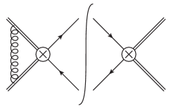
(a)

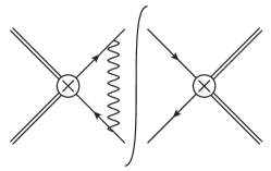
(b)

Figure 1: Relevant Feynman diagrams for the virtual part of the TMDShF. Double solid lines stand for soft Wilson lines, while single lines for heavy quarks. The gluon in diagram 1a is soft, while the one in diagram 1b, denoted with a wavy line, is ultrasoft. Corresponding crossed diagrams should be added.

The one-loop virtual part of the renormalized TMDShF, defined in (17), is given by the virtual diagrams of the bare TMDShF in figure 1 and the ones of the soft function. On one hand, diagram 1a (and its crossed one) gives exactly the same as the corresponding one for the soft function $S$, and thus it is cancelled in ${\tilde{S}}_{\cal Q}$. On the other, diagram 1b (and its crossed one) is analogous to the one found in the long-distance matrix element (LDME) $\left<0\right|\chi^{\dagger}\psi\,a_{\eta_{Q}}^{\dagger}a_{\eta_{Q}}\,\psi^{\dagger}\chi\left|0\right>$, and can thus be obtained e.g. from Petrelli:1997ge ; Jia:2011ah . Putting everything together, the result is:

$${\tilde{S}}_{\mathcal{Q}}\Big{|}_{v} =1+\frac{\alpha_{s}}{2\pi}C_{F}\frac{\pi^{2}}{v}\,.$$ (30)

Notice that the heavy-quark self-energy vanishes on the energy shell (see e.g. Bodwin:1994jh ). In addition, there are no interactions at this order between the heavy quarks (soft) and the soft gluons from the soft Wilson lines Luke:1999kz . In fact, the gluon connecting the two soft Wilson lines in diagram 1a is soft, while the one connecting the heavy quarks in diagram 1b is ultrasoft. This is the reason why the authors in Ma:2012hh ; Ma:2015vpt get to the misleading conclusion that the factorization ansatz they propose for this process is justified, i.e., that the cross-section is given in terms of two (subtracted) gluon TMDs and the local LDME, which they claim is completely factorized from the soft function at low transverse momentum. Indeed, it turns out that, at one-loop, the virtual part of the TMDShF $S_{\mathcal{Q}}$ is given by the virtual part of the local LDME. However this fact does not hold for higher-orders. The TMDShF at low transverse momentum is a genuine non-perturbative quantity.

Finally, subtracting to the virtual part of the cross-section in full QCD the virtual part of two gluon TMDs and the virtual part of the TMDShF, we obtain the hard part up to ${\mathcal{O}}(\alpha_{s})$:

$$H =1+\frac{\alpha_{s}}{2\pi}\Bigg{[}-C_{A}\hbox{ln}^{2}\frac{\mu^{2}}{M^{2}}-C_{A}\frac{\pi^{2}}{6}+2B_{{}^{1}S_{0}}^{[1]}\Bigg{]}\,,$$ (31)

As expected, this coefficient turns out to be free from infrared divergences, which means that the derived factorization theorem properly reproduces the infrared part of the cross-section in full QCD at one loop. This constitutes a non-trivial consistency check. In addition, this coefficient is a necessary ingredient for the resummation of large logarithms at higher orders, allowing for precise phenomenological studies in the near future.

IV Conclusions

By applying the effective field theory approach, a proper factorization theorem for $\eta_{c,b}$ hadro-production at low transverse momentum is derived, finding a new kind of non-perturbative hadronic quantity: the TMD shape function (TMDShF). This matrix element encodes the two soft mechanisms present in the process, the formation of the heavy-quark bound state and the soft-gluon radiation, which were assumed to factorize in all previous works in the literature.

In general, there are as many TMDShFs for a given process as relevant angular/color Fock states within NRCQD power counting. Simply stated, they could be considered the TMD extensions of the well-known LDMEs.

Quarkonium production processes can thus be used to access gluon TMDs, but the phenomenology is more involved as compared to quark TMDs in, e.g., Drell-Yan or semi-inclusive deep-inelastic scattering processes, since it requires in addition the parametrization of several TMDShFs.

These findings can straightforwardly be applied to other quarkonia production processes, for instance in lepton-hadron collisions (like $ep\to J/\psi$) or electron-positron annihilation (like $e^{+}e^{-}\to J/\psi\pi$). This is left for a future effort.

References

- (1) R. Angeles-Martinez et al., “Transverse Momentum Dependent (TMD) parton distribution functions: status and prospects,” Acta Phys. Polon. B46 no. 12, (2015) 2501–2534, arXiv:1507.05267 [hep-ph].
- (2) A. Accardi et al., “Electron Ion Collider: The Next QCD Frontier,” Eur. Phys. J. A52 no. 9, (2016) 268, arXiv:1212.1701 [nucl-ex].
- (3) C. Hadjidakis et al., “A Fixed-Target Programme at the LHC: Physics Case and Projected Performances for Heavy-Ion, Hadron, Spin and Astroparticle Studies,” arXiv:1807.00603 [hep-ex].
- (4) D. Kikola, M. G. Echevarria, C. Hadjidakis, J.-P. Lansberg, C. Lorcé, L. Massacrier, C. M. Quintans, A. Signori, and B. Trzeciak, “Feasibility Studies for Single Transverse-Spin Asymmetry Measurements at a Fixed-Target Experiment Using the LHC Proton and Lead Beams (AFTER@LHC),” Few Body Syst. 58 no. 4, (2017) 139, arXiv:1702.01546 [hep-ex].
- (5) B. Trzeciak, C. Da Silva, E. G. Ferreiro, C. Hadjidakis, D. Kikola, J. P. Lansberg, L. Massacrier, J. Seixas, A. Uras, and Z. Yang, “Heavy-ion Physics at a Fixed-Target Experiment Using the LHC Proton and Lead Beams (AFTER@LHC): Feasibility Studies for Quarkonium and Drell-Yan Production,” Few Body Syst. 58 no. 5, (2017) 148, arXiv:1703.03726 [nucl-ex].
- (6) S. J. Brodsky, F. Fleuret, C. Hadjidakis, and J. P. Lansberg, “Physics Opportunities of a Fixed-Target Experiment using the LHC Beams,” Phys. Rept. 522 (2013) 239–255, arXiv:1202.6585 [hep-ph].
- (7) M. G. Echevarria, A. Idilbi, and I. Scimemi, “Factorization Theorem For Drell-Yan At Low And Transverse Momentum Distributions On-The-Light-Cone,” JHEP 07 (2012) 002, arXiv:1111.4996 [hep-ph].
- (8) M. G. Echevarria, A. Idilbi, A. Schäfer, and I. Scimemi, “Model-Independent Evolution of Transverse Momentum Dependent Distribution Functions (TMDs) at NNLL,” Eur. Phys. J. C73 no. 12, (2013) 2636, arXiv:1208.1281 [hep-ph].
- (9) M. G. Echevarría, A. Idilbi, and I. Scimemi, “Soft and Collinear Factorization and Transverse Momentum Dependent Parton Distribution Functions,” Phys. Lett. B726 (2013) 795–801, arXiv:1211.1947 [hep-ph].
- (10) M. G. Echevarria, A. Idilbi, and I. Scimemi, “Unified treatment of the QCD evolution of all (un-)polarized transverse momentum dependent functions: Collins function as a study case,” Phys. Rev. D90 no. 1, (2014) 014003, arXiv:1402.0869 [hep-ph].
- (11) J. Collins, “Foundations of perturbative QCD,” Camb. Monogr. Part. Phys. Nucl. Phys. Cosmol. 32 (2011) 1–624.
- (12) D. Gutierrez-Reyes, S. Leal-Gomez, I. Scimemi, and A. Vladimirov, “Linearly polarized gluons at next-to-next-to leading order and the Higgs transverse momentum distribution,” arXiv:1907.03780 [hep-ph].
- (13) D. Gutierrez-Reyes, I. Scimemi, and A. Vladimirov, “Transverse momentum dependent transversely polarized distributions at next-to-next-to-leading-order,” JHEP 07 (2018) 172, arXiv:1805.07243 [hep-ph].
- (14) M. G. Echevarria, I. Scimemi, and A. Vladimirov, “Unpolarized Transverse Momentum Dependent Parton Distribution and Fragmentation Functions at next-to-next-to-leading order,” JHEP 09 (2016) 004, arXiv:1604.07869 [hep-ph].
- (15) M. G. Echevarria, I. Scimemi, and A. Vladimirov, “Universal transverse momentum dependent soft function at NNLO,” Phys. Rev. D93 no. 5, (2016) 054004, arXiv:1511.05590 [hep-ph].
- (16) M. G. Echevarria, I. Scimemi, and A. Vladimirov, “Transverse momentum dependent fragmentation function at next-to–next-to–leading order,” Phys. Rev. D93 no. 1, (2016) 011502, arXiv:1509.06392 [hep-ph]. [Erratum: Phys. Rev.D94,no.9,099904(2016)].
- (17) U. D’Alesio, M. G. Echevarria, S. Melis, and I. Scimemi, “Non-perturbative QCD effects in spectra of Drell-Yan and Z-boson production,” JHEP 11 (2014) 098, arXiv:1407.3311 [hep-ph].
- (18) M. G. Echevarria, A. Idilbi, Z.-B. Kang, and I. Vitev, “QCD Evolution of the Sivers Asymmetry,” Phys. Rev. D89 (2014) 074013, arXiv:1401.5078 [hep-ph].
- (19) A. Bacchetta, M. G. Echevarria, P. J. G. Mulders, M. Radici, and A. Signori, “Effects of TMD evolution and partonic flavor on e+ e- annihilation into hadrons,” JHEP 11 (2015) 076, arXiv:1508.00402 [hep-ph].
- (20) A. Bacchetta, F. Delcarro, C. Pisano, M. Radici, and A. Signori, “Extraction of partonic transverse momentum distributions from semi-inclusive deep-inelastic scattering, Drell-Yan and Z-boson production,” JHEP 06 (2017) 081, arXiv:1703.10157 [hep-ph]. [Erratum: JHEP06,051(2019)].
- (21) M. Anselmino, M. Boglione, U. D’Alesio, F. Murgia, and A. Prokudin, “Study of the sign change of the Sivers function from STAR Collaboration W/Z production data,” JHEP 04 (2017) 046, arXiv:1612.06413 [hep-ph].
- (22) I. Scimemi and A. Vladimirov, “Analysis of vector boson production within TMD factorization,” Eur. Phys. J. C78 no. 2, (2018) 89, arXiv:1706.01473 [hep-ph].
- (23) V. Bertone, I. Scimemi, and A. Vladimirov, “Extraction of unpolarized quark transverse momentum dependent parton distributions from Drell-Yan/Z-boson production,” JHEP 06 (2019) 028, arXiv:1902.08474 [hep-ph].
- (24) M. G. Echevarria, T. Kasemets, P. J. Mulders, and C. Pisano, “QCD evolution of (un)polarized gluon TMDPDFs and the Higgs -distribution,” JHEP 07 (2015) 158, arXiv:1502.05354 [hep-ph]. [Erratum: JHEP05,073(2017)].
- (25) R. M. Godbole, A. Misra, A. Mukherjee, and V. S. Rawoot, “Sivers Effect and Transverse Single Spin Asymmetry in ,” Phys. Rev. D85 (2012) 094013, arXiv:1201.1066 [hep-ph].
- (26) D. Boer and C. Pisano, “Polarized gluon studies with charmonium and bottomonium at LHCb and AFTER,” Phys. Rev. D86 (2012) 094007, arXiv:1208.3642 [hep-ph].
- (27) R. M. Godbole, A. Misra, A. Mukherjee, and V. S. Rawoot, “Transverse Single Spin Asymmetry in and Transverse Momentum Dependent Evolution of the Sivers Function,” Phys. Rev. D88 no. 1, (2013) 014029, arXiv:1304.2584 [hep-ph].
- (28) R. M. Godbole, A. Kaushik, A. Misra, and V. S. Rawoot, “Transverse single spin asymmetry in and evolution of Sivers function-II,” Phys. Rev. D91 no. 1, (2015) 014005, arXiv:1405.3560 [hep-ph].
- (29) G.-P. Zhang, “Probing transverse momentum dependent gluon distribution functions from hadronic quarkonium pair production,” Phys. Rev. D90 no. 9, (2014) 094011, arXiv:1406.5476 [hep-ph].
- (30) G.-P. Zhang, “Transverse momentum dependent gluon fragmentation functions from production at colliders,” Eur. Phys. J. C75 no. 10, (2015) 503, arXiv:1504.06699 [hep-ph].
- (31) A. Mukherjee and S. Rajesh, “Probing Transverse Momentum Dependent Parton Distributions in Charmonium and Bottomonium Production,” Phys. Rev. D93 no. 5, (2016) 054018, arXiv:1511.04319 [hep-ph].
- (32) A. Mukherjee and S. Rajesh, “ production in polarized and unpolarized ep collision and Sivers and asymmetries,” Eur. Phys. J. C77 no. 12, (2017) 854, arXiv:1609.05596 [hep-ph].
- (33) A. Mukherjee and S. Rajesh, “Linearly polarized gluons in charmonium and bottomonium production in color octet model,” Phys. Rev. D95 no. 3, (2017) 034039, arXiv:1611.05974 [hep-ph].
- (34) D. Boer, “Gluon TMDs in quarkonium production,” Few Body Syst. 58 no. 2, (2017) 32, arXiv:1611.06089 [hep-ph].
- (35) J.-P. Lansberg, C. Pisano, and M. Schlegel, “Associated production of a dilepton and a at the LHC as a probe of gluon transverse momentum dependent distributions,” Nucl. Phys. B920 (2017) 192–210, arXiv:1702.00305 [hep-ph].
- (36) R. M. Godbole, A. Kaushik, A. Misra, V. Rawoot, and B. Sonawane, “Transverse single spin asymmetry in ,” Phys. Rev. D96 no. 9, (2017) 096025, arXiv:1703.01991 [hep-ph].
- (37) U. D’Alesio, F. Murgia, C. Pisano, and P. Taels, “Probing the gluon Sivers function in and ,” Phys. Rev. D96 no. 3, (2017) 036011, arXiv:1705.04169 [hep-ph].
- (38) S. Rajesh, R. Kishore, and A. Mukherjee, “Sivers effect in Inelastic Photoproduction in Collision in Color Octet Model,” Phys. Rev. D98 no. 1, (2018) 014007, arXiv:1802.10359 [hep-ph].
- (39) A. Bacchetta, D. Boer, C. Pisano, and P. Taels, “Gluon TMDs and NRQCD matrix elements in production at an EIC,” arXiv:1809.02056 [hep-ph].
- (40) J.-P. Lansberg, C. Pisano, F. Scarpa, and M. Schlegel, “Pinning down the linearly-polarised gluons inside unpolarised protons using quarkonium-pair production at the LHC,” Phys. Lett. B784 (2018) 217–222, arXiv:1710.01684 [hep-ph]. [Erratum: Phys. Lett.B791,420(2019)].
- (41) R. Kishore and A. Mukherjee, “Accessing linearly polarized gluon distribution in production at the electron-ion collider,” Phys. Rev. D99 no. 5, (2019) 054012, arXiv:1811.07495 [hep-ph].
- (42) F. Scarpa, D. Boer, M. G. Echevarria, J.-P. Lansberg, C. Pisano, and M. Schlegel, “Studies of gluon TMDs and their evolution using quarkonium-pair production at the LHC,” arXiv:1909.05769 [hep-ph].
- (43) P. Sun, C. P. Yuan, and F. Yuan, “Heavy Quarkonium Production at Low Pt in NRQCD with Soft Gluon Resummation,” Phys. Rev. D88 (2013) 054008, arXiv:1210.3432 [hep-ph].
- (44) J. P. Ma, J. X. Wang, and S. Zhao, “Transverse momentum dependent factorization for quarkonium production at low transverse momentum,” Phys. Rev. D88 no. 1, (2013) 014027, arXiv:1211.7144 [hep-ph].
- (45) J. P. Ma, J. X. Wang, and S. Zhao, “Breakdown of QCD Factorization for P-Wave Quarkonium Production at Low Transverse Momentum,” Phys. Lett. B737 (2014) 103–108, arXiv:1405.3373 [hep-ph].
- (46) J. P. Ma and C. Wang, “QCD factorization for quarkonium production in hadron collisions at low transverse momentum,” Phys. Rev. D93 no. 1, (2016) 014025, arXiv:1509.04421 [hep-ph].
- (47) C. W. Bauer, S. Fleming, and M. E. Luke, “Summing Sudakov logarithms in B —¿ X(s gamma) in effective field theory,” Phys. Rev. D63 (2000) 014006, arXiv:hep-ph/0005275 [hep-ph].
- (48) C. W. Bauer, S. Fleming, D. Pirjol, and I. W. Stewart, “An Effective field theory for collinear and soft gluons: Heavy to light decays,” Phys. Rev. D63 (2001) 114020, arXiv:hep-ph/0011336 [hep-ph].
- (49) C. W. Bauer and I. W. Stewart, “Invariant operators in collinear effective theory,” Phys. Lett. B516 (2001) 134–142, arXiv:hep-ph/0107001 [hep-ph].
- (50) C. W. Bauer, D. Pirjol, and I. W. Stewart, “Soft collinear factorization in effective field theory,” Phys. Rev. D65 (2002) 054022, arXiv:hep-ph/0109045 [hep-ph].
- (51) C. W. Bauer, S. Fleming, D. Pirjol, I. Z. Rothstein, and I. W. Stewart, “Hard scattering factorization from effective field theory,” Phys. Rev. D66 (2002) 014017, arXiv:hep-ph/0202088 [hep-ph].
- (52) M. Beneke, A. P. Chapovsky, M. Diehl, and T. Feldmann, “Soft collinear effective theory and heavy to light currents beyond leading power,” Nucl. Phys. B643 (2002) 431–476, arXiv:hep-ph/0206152 [hep-ph].
- (53) G. T. Bodwin, E. Braaten, and G. P. Lepage, “Rigorous QCD analysis of inclusive annihilation and production of heavy quarkonium,” Phys. Rev. D51 (1995) 1125–1171, arXiv:hep-ph/9407339 [hep-ph]. [Erratum: Phys. Rev.D55,5853(1997)].
- (54) A. Idilbi and I. Scimemi, “Singular and Regular Gauges in Soft Collinear Effective Theory: The Introduction of the New Wilson Line T,” Phys. Lett. B695 (2011) 463–468, arXiv:1009.2776 [hep-ph].
- (55) M. Garcia-Echevarria, A. Idilbi, and I. Scimemi, “SCET, Light-Cone Gauge and the T-Wilson Lines,” Phys. Rev. D84 (2011) 011502, arXiv:1104.0686 [hep-ph].
- (56) J. Collins and J.-W. Qiu, “ factorization is violated in production of high-transverse-momentum particles in hadron-hadron collisions,” Phys. Rev. D75 (2007) 114014, arXiv:0705.2141 [hep-ph].
- (57) J. Collins, “2-soft-gluon exchange and factorization breaking,” arXiv:0708.4410 [hep-ph].
- (58) T. C. Rogers and P. J. Mulders, “No Generalized TMD-Factorization in Hadro-Production of High Transverse Momentum Hadrons,” Phys. Rev. D81 (2010) 094006, arXiv:1001.2977 [hep-ph].
- (59) D. Boer, S. Cotogno, T. van Daal, P. J. Mulders, A. Signori, and Y.-J. Zhou, “Gluon and Wilson loop TMDs for hadrons of spin 1,” JHEP 10 (2016) 013, arXiv:1607.01654 [hep-ph].
- (60) A. Petrelli, M. Cacciari, M. Greco, F. Maltoni, and M. L. Mangano, “NLO production and decay of quarkonium,” Nucl. Phys. B514 (1998) 245–309, arXiv:hep-ph/9707223 [hep-ph].
- (61) Y. Jia, X.-T. Yang, W.-L. Sang, and J. Xu, “ correction to pseudoscalar quarkonium decay to two photons,” JHEP 06 (2011) 097, arXiv:1104.1418 [hep-ph].
- (62) M. E. Luke, A. V. Manohar, and I. Z. Rothstein, “Renormalization group scaling in nonrelativistic QCD,” Phys. Rev. D61 (2000) 074025, arXiv:hep-ph/9910209 [hep-ph].