Reconstructing solar magnetic fields from historical observations

Abstract

Context. Systematic observations of magnetic field strength and polarity in sunspots began at Mount Wilson Observatory (MWO), USA in early 1917. Except for a few brief interruptions, this historical dataset has continued until the present.

Aims. Sunspot field strength and polarity observations are critical in our project of reconstructing the solar magnetic field over the last hundred years. We provide a detailed description of the newly digitized dataset of drawings of sunspot magnetic field observations.

Methods. The digitization of MWO drawings is based on a software package that we developed. It includes a semiautomatic selection of solar limbs and other features of the drawing, and a manual entry of the time of observations, measured field strength, and other notes handwritten on each drawing. The data are preserved in an MySQL database.

Results. We provide a brief history of the project and describe the results from digitizing this historical dataset. We also provide a summary of the final dataset and describe its known limitations. Finally, we compare the sunspot magnetic field measurements with those from other instruments, and demonstrate that, if needed, the dataset could be continued using modern observations such as, for example, the Vector Stokes Magnetograph on the Synoptic Optical Long-term Investigations of the Sun platform.

1 Introduction

In 1896, the Dutch physicist Pieter Zeeman conducted a series of experiments that led to the discovery that in the presence of strong magnetic fields some spectral lines split into multiple components. Later the same year, Hendrik Lorentz proposed a theoretical explanation of these observations based on his theory of electromagnetic radiation. In 1902, Zeeman and Lorentz shared the Nobel Prize for the discovery and explanation of a fundamental physical effect we now refer to as the Zeeman effect. In the concluding section of the article describing his experiments on spectral line splitting and polarization, Zeeman posed a question about a possible effect of then hypothesized magnetic fields on the Sun (Zeeman 1897). In 1908, American astronomer George E. Hale (Hockey et al. 2014) discovered the presence of the magnetic field in sunspots. Figure 1a shows an example of a spectral line splitting in the presence of a strong magnetic field in a sunspot. While the discovery of the magnetic field in sunspots is usually credited to Hale’s 1908 paper (Hale 1908), it was, in fact, a combination of formal articles and personal communications (including short telegrams) between Hale and Zeeman that led to a discovery of both the longitudinal (along the line of sight) and transverse (orthogonal to the line of sight) magnetic fields in sunspots. The broadening pattern in spectral lines characteristic to the Zeeman effect was first observed by other astronomers (e.g., Mitchell 1906), who, unlike Hale, failed to properly interpret the observations in terms of magnetic fields. Additional information on the history of the discovery of magnetic fields on the Sun is provided in Bakker (1946); Spencer (1965); Harvey (1999); del Toro Iniesta (1996); Stenflo (2017).

Early observations conducted in 1908 indicated that a proper measurement of sunspot magnetic fields requires a telescope with a large image size in the focal plane (which implies a longer focal length), and a spectrograph with a high resolving power. In 1909, the Carnegie Institution of Washington provided the necessary funding for the construction of a new 150 feet (45.7 meters) tower telescope at the Mount Wilson Observatory (MWO) in California. The construction of the tower was completed in 1910 and the first observations were taken in 1911. The construction project was finished in May 1912 with the completion of the Littrow spectrograph (Howard 1985). Meanwhile, studies of the magnetic field on the Sun continued with such important findings as a possible height dependence of sunspot field strengths, the recognition of the bipolar structure of active regions (Hale 1910), and even with a claim about the presence of a global dipolar magnetic field on the Sun (Hale 1913). The validity of the latter finding was questioned by some later researchers (e.g., Stenflo 2017) and, indeed, based on current knowledge, the mean strength of the polar field derived by Hale may appear too large. Nevertheless, the measurements showed a hemispheric asymmetry in the polarity of magnetic fields at middle and high latitudes. Since these field values were longitudinal averages over a range of latitudes, we could speculate that these measurements might represent the imbalance of large-scale magnetic fields of decaying active regions. Then the derived field strengths may not be so unreasonable after all.

With the completion of the 150 feet solar tower telescope, the MWO synoptic program of daily sunspot drawings including the measurements of sunspot polarities and field strengths began in 1917 with the first measurements made by Ferdinand Ellerman (Hockey et al. 2014) on 4 January 1917. With a few interruptions due to funding issues, this program has continued until the present. In the fall of 1978, water from severe rainfalls flooded the spectrograph and partially damaged the spectrograph grating and the lens. As a precaution, all following gratings were installed in a watertight box. In 1984, the Carnegie Institution of Washington made a decision to close the MWO. In late 1985, a memorandum of understanding was signed between the Carnegie Institution and the University of California in Los Angeles (UCLA), allowing the continuation of the sunspot drawing program. The primary objective of the funded program was the study of dynamical structures such as the torsional oscillations, which required multiple magnetogram or Dopplergram observations throughout the day. During the peak of the solar cycle, the drawings occupied two hours or more to complete, leading to the loss of observations for the primary program. Consequently, daily observations were stopped on 15 September 2004. In 2005, only nine drawings were made, and in 2006, there were only two drawings. The daily observations restarted on 25 January 2007 with the compromise that the magnetic field in the smaller spots would not be measured. The most recent observations, however, are made on a volunteer basis by longtime observer Steve Padilla. Thus, they could stop at any time.

Manual measurements of sunspot field strengths using the approach pioneered by Hale were conducted at several other observatories, such as Potsdam, Rome, and the Crimean Astrophysical Observatory (CrAO) (see Livingston et al. 2006). Another notable synoptic dataset comes from the network of observatories in the former Soviet Union, which operated within the framework of the Solar Service program (Pevtsov et al. 2011). This latter dataset extends from early 1950s through late 1990s. After 1998, it has continued based on daily observations from a single station (CrAO).

In the mid-2000s to early 2010s, a series of papers related to the long-term variation of sunspot field strengths rejuvenated the interest in the MWO synoptic dataset (Penn & Livingston 2006, 2011; Pevtsov et al. 2011; Watson et al. 2011; Rezaei et al. 2012; Nagovitsyn et al. 2012; Livingston et al. 2012; Pevtsov et al. 2014; Lockwood et al. 2014; Rezaei et al. 2015; Tlatova et al. 2015). This renewed interest led to our present collaborative effort in digitizing the Mount Wilson sunspot drawings. As this project enters its final stage, we feel obligated to provide a detailed description of the resulting dataset. In Section 2 we describe the concept of measuring the magnetic fields employed by Hale and provide a history of instrument changes. In Section 3 we summarize the steps taken in the course of drawing digitization and outline the features of the searchable database of sunspot field strengths that we created. Sections 4–5 provide critical discussions of data quality, the estimate of uncertainties, and the known issues. Because of an inevitable termination of the current sunspot drawings program at MWO, a possible continuation of this time series using modern Stokes polarimeter data has been developed at the National Solar Observatory (NSO) (Hughes et al. 2013). This method relies on measuring the Zeeman splitting in Stokes $I$ and $V$ profiles, and it closely mimics the original approach by Hale. Section 6 provides a brief summary of that approach and compares the derived field strengths with those from the MWO manual measurements.

2 Method and observations

A daily observation of sunspot field strengths starts by the observer creating a full disk drawing of sunspots. Next, the observer centers each spot on the spectrograph slit and takes the measurement. Figure 1 provides a graphical explanation of the measuring steps. The spectrograph is equipped with a device that contains two strips of optical retarders (quarter-wavelength plates) placed above each other in the direction along the spectrograph slit. The two retarders have their primary axes at a 90-degree angle with respect to each other and are set to be at 45 degrees to the prime axis of the Nicol prism polarizer situated behind the retarders (Figure 1b). The detailed description of this setup can be found in Hale (1913); Ellerman (1919); Hale & Nicholson (1938). In the presence of a longitudinal magnetic field in the solar photosphere, a spectral line (sensitive to the presence of the magnetic field) splits into two components, in which one component has a left-hand circular polarization and the other component is circularly polarized in the right-hand sense. The polarization pattern depends on the polarity of the magnetic field. Passing through the quarter wavelength plate converts the circularly polarized light to linearly polarized with two orthogonal orientations, which are spatially separated by the Nicol prism. In the absence of a transverse component, the observer sees the two components of the Zeeman triplet above each other, spatially shifted relative to each other (Figure 1d). The above setup has no significant effect if the incoming light has linear polarization due to transverse Zeeman effect. For linear polarization, the central $\pi$ component of spectral line is visible in both spectra, as depicted in Figure 1c.

The separation between two $\sigma$ components represents the total field strength. The polarization pattern of the components (circular, linear, or a mix of both – elliptical) contains information about the orientation of the magnetic field vector relative to the line of sight. Thus, the linear separation $\Delta x$ (mm) between the two circularly polarized $\sigma$ components can be used to measure the (total) field strength, $B$ (G) as follows:

$$B=\frac{s\leavevmode\nobreak\ \Delta x\cdot 10^{13}}{9.34\cdot g\leavevmode\nobreak\ \lambda^{2}},$$ (1)

where $\lambda$ is the wavelength (in Å), $g$ is Landè factor, and $s$ is the linear dispersion (Å/mm; see Eq. 4).

To measure the separation $\Delta x$ between the two $\sigma$ components of the spectral line, the spectrograph is equipped with a transparent (glass) plane-parallel plate (the so-called tip plate), which can be tilted (Figure 1e). Light from the low part of the spectrum passes through this tip plate, and tipping the plate allows the observer to align the two $\sigma$ components (Figure 1f, g). Equation 2 shows the relation between the rotation angle $\alpha$ of the tip plate and the lateral separation $\Delta$x of spectra, i.e.,

$$\Delta x=t\cdot\sin\alpha\leavevmode\nobreak\ \Bigg{(}1-\frac{\cos\alpha}{\sqrt{n^{2}-\sin^{2}\alpha}}\leavevmode\nobreak\ \Bigg{)},$$ (2)

where $t$ is the thickness of the plate and $n$ is its index of refraction. The rotation angle $\alpha$ is calibrated to $\Delta$x, and, typically, the values are written in a look-up table for the observer to translate the tip angle into the corresponding field strength. The polarity of the magnetic field is determined from the direction of the lateral shift required to align the $\sigma$ component in the lower part of spectra with the upper part (see Figure 1g). In the early period of MWO observations, instead of look-up tables, the observer used the tip angle directly as the measure of the field strength; i.e., the angle in degrees corresponded to a field strength in units of 100 G. For example, 10$\degr$ would correspond to 1000 G, 25$\degr$ would be recorded as 2500 G, etc. Using a tip plate as the measuring device has two disadvantages. First, the dependence between the tip angle and the lateral shift is nonlinear (Equation 2). The nonlinearity is relatively small for small tip angles, but it increases rapidly for large angles. Second, the range of measurements is restricted by the maximum tip angle of the plate (about 60$\degr$). This limits the maximum field strength that could be measured.

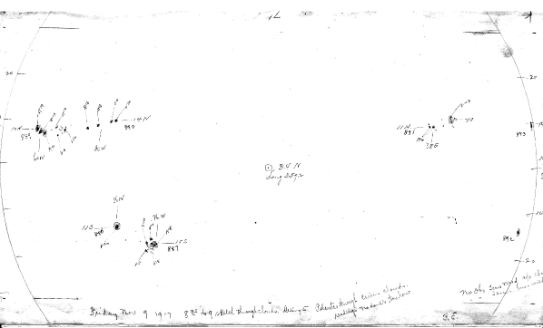
Figure 2: (a) Example of a typical sunspot drawing from the MWO dataset taken on 9 November 1917 between 8:35 and 9:00 (local time). Measured sunspot field strengths are shown in units of hundred G and their polarities designated as “R” and “V” (for red and violet, which corresponds to the positive and the negative polarities). Credit: Carnegie Observatories.

Figure 2 provides an example of one of the earliest sunspot drawings. For each sunspot, the observer would draw the umbra and penumbra; the umbra is shown as the dark-shaded area and the penumbra is shown as a light-shaded area or outlined by a contour. In addition to the sunspots, their magnetic polarity and field strength, the drawings show the location of the solar disk center with its approximate latitude (solar B-angle) and the solar limbs. Other notations on the drawings include the date and time of observations, the atmospheric seeing conditions (smaller number corresponds to poorer seeing conditions), and the observer’s initials. While the characterization of the seeing conditions is subjective, for a reference we note that, based on a personal experience of one of the coauthors, the observations denoted as “Seeing 3” were taken on a partially cloudy day with the solar granulation clearly visible. The seeing scale is between 1 and 5.

Some drawings may include other handwritten notes either related to the observations (e.g., indicating that some sunspots were measured on a different day owing to the weather condition), or even personal notes; for example, there is a note about the first observations, taken with the then world’s largest 100 inch (2.5 m) Hooker telescope, planet Mercury transit on 7 May 1924. Many drawings made during the first two months after the project started are not annotated with field strengths However, the same drawings published in Hale & Nicholson (1938) show field strengths measured in these sunspots. We think that for the early period, the measured field strengths were not written on the drawings, but were perhaps recorded in some other way. Since our database is based on information from drawings, these cases are currently not included.

The quality of the drawings shows a significant evolution over the period of the program. Hale & Nicholson (1938), in their reference to 1917–1924 period, indicated that the drawings should be considered as approximate, chiefly for the purpose of the identification of sunspots for which the measurements were taken. Indeed, the drawings from that early period appear to be less rich in detail, and may often not even show multiple umbrae inside sunspots. In contrast, the more recent drawings exhibit an extremely high degree of detail and, while they look like photographs, in some respect they are even better, as a skilled observer can draw the details based on moments of clearer seeing. The level of details in drawings made in other periods vary between these two extremes. Normally, it takes about 10-15 minutes for the current observer to complete the drawing, but the notes written on drawings suggest that sometimes it took longer (e.g., because of clouds or rapid changes in weather). Perhaps as an indication of uncertainty in time of observations, the observers sometimes recorded the time of observations rounded to the closest 15 minutes. This time quantization could be identified from the beginning of observations, but it became universally adopted after about 1979. Cases when the drawing had to be interrupted and completed at a later time are normally indicated with the appropriate time of observations for each group of features. Nevertheless, the users of these drawings need to understand that the locations of sunspots on a drawing are not recorded exactly simultaneously, and the features may have slightly shifted from the location corresponding to the indicated time of drawing as a consequence of solar rotation.

The drawings contain a sign of a developed understanding of new solar phenomena. For example, the early measurements had uncovered a possible polarity reversal of the magnetic field of sunspots situated near the solar limb. It was clearly studied in detail as the drawings from that time period would often exhibit a line dividing sunspots into two parts, with the field strength and the polarity measured in each part (e.g., 15 January 1918, sunspots near the east-north limb). Some drawings may show a set of lines across the sunspot with the measurements taken along each line across the sunspot (e.g., 22 July 1918). It appears that at some point, the origin of this phenomenon was finally understood (Hale et al. 1919), and drawings after that time no longer include such details. As we know now, this effect is due to a projection of a fan-like structure of magnetic field in a sunspot onto the line-of-sight direction. The database includes both measurements of the main polarity and the polarity appearing due to projection.

As other example, drawing taken on 19 November 1921 shows marks for measured magnetic field to the west of a large unipolar sunspot. This was the result of a search for “invisible” sunspots of opposite polarity next to unipolar spots (Hale 1922). The database does not include these measurements outside sunspot or pores.

Initially, the observations were taken in spectral line Fe I 6173.343 Å (Landé factor g=2.5). Hale & Nicholson (1938) quoted the width of the spectrograph entrance slit as 76 $\mu$m, and the observations were taken in the second spectral order of the spectrograph. This slit width is close to the normal slit width, which is the minimum width that maximizes the resolving power of the spectrograph without sacrificing the intensity of spectra. An examination of observer logbooks indicates that there was no standard protocol for recording such information as the spectrograph settings and, when changes were made, they could be recorded in various ways (or were not recorded at all). Thus, for example, Ulrich et al. (1991) reported that for sunspot field strength measurements a slit of 356 $\mu$m width is used. Recent examination of the slit width has revealed an even larger width of about 500 $\mu$m; there is no recording of when this change was made. This indicates that the slit adjustments were not well documented.

Beginning October 1961, the observations were switched to the spectral line Fe I 5250.217 Å with the Landé factor of g= 3.0. The measurements were made in the fifth spectral order. This switch required replacing the previous 4 mm thick tip plate (with the index of refraction of $n$ = 1.521 for crown glass) by a thicker tip plate of 7 mm (with the index of refraction of $n$ = 1.461 for fused silica). This replacement introduced the limitation on the maximum strength of magnetic field that could be measured to approximately 3000 G.

There were nine spectral gratings over the lifetime of the project. Properties of these gratings are summarized in Table 1; additional details can be found in Livingston et al. (2006). Spectral orders are not well recorded in observer logs. Thus, we estimated spectral orders on the basis of scaling used to convert tip angles to gauss and the linear dispersion computed by us using parameters of gratings. The spectrograph grating equation for the Littrow configuration could be written as

$$m\lambda=2d\leavevmode\nobreak\ \sin\beta,$$ (3)

where $\beta$ is angle of diffraction, $m$ is the spectral (diffraction) order, $d$ is the spacing between the grooves (i.e., $d^{-1}$ represents a more familiar measure of number of grooves per millimeter), and $\lambda$ is the wavelength. The linear dispersion ($s$) is

$$s=\frac{\partial\lambda}{\partial x}=\frac{d\leavevmode\nobreak\ \cos\beta}{mL},$$ (4)

where $L$ = 22.9 m is the effective focal length of the spectrograph. Using Equations 3 and 4 we computed the linear dispersion for all spectral gratings employed in the course of MWO sunspot field strength project. Table 1 shows the measured magnetic field strengths (100 G, 1000 G, 2000 G, 3000 G, and 4000 G) and the “true” strengths that were computed using Equations 1-2. The true field strengths are rounded to the nearest 10 G. For measurements taken after 1961, the true field strengths that require tip angles in the excess of 60$\degr$ are not shown in Table 1. For measurements taken after 1994, the lookup table was used. The lookup table does not include values for tip angles smaller than 22$\degr$ and thus the entry for 100 G in Table 1 is not shown.

While these calculations should be considered as approximations, they clearly demonstrate that the measuring method adopted at MWO slightly overestimates the weaker field strengths, and it could significantly underestimate the strong magnetic fields. As noted by Livingston et al. (2006), before 1961 the linear dispersion in the observing wavelength range changed very little, and the resulting differences between the measured and true fields (computed from the Equations 1- 2) are within 100 G (with the exception of strongest fields $\ga$ 3500 G; see also, Table 1). After October 1961, when the observations switched to the spectral line Fe I 525.0217 nm (and the 7 mm tip plate), the measuring method was to divide the tip angle by two and round to it to the nearest degree (Livingston et al. 2006). Analyzing Equation 2) suggests that this method works reasonably well for gratings no. 6–8 and for field strengths $\la$ 2000 G. During this period, there is a strong nonlinearity for magnetic fields in the range 2500-3000 G (measured fields). For observations taken after 1994 (grating no. 9), a lookup table was used to convert the tip angles to the field strengths. The lookup table, which is currently (2018) used for the observations is shown in Table 2. For comparison, we show the range of true values of magnetic fields corresponding to the measured fields and rounded to the nearest 100 G. Livingston et al. (2006) noted that the lookup table of measured field values overestimates the weaker fields ($\la$ 2200 G) and underestimates stronger fields ($\ga$2700 G). For data taken during this period, Livingston et al. (2006) proposed corrections for the measured field strengths. For 1917-1961 period, our calculations for true field strength agree with Livingston et al. (2006). In reference to post-1994 measurements using the lookup table, Livingston et al. (2006) wrote that for the maximum tip angle of 60$\degr$, the lookup table indicates 2600 G while the true field strength is about 2960 G. Our calculations for this case, rounded to the nearest 10 G also show 2960 G. However, for measurements during 1961–1994, Livingston et al. (2006) listed only a single correction, while there were three different spectral gratings with slightly different linear dispersion. Thus, for example, the correction Table II in Livingston et al. (2006) showed that the published field of 3000 G corresponds to true field of 3800 G. Our calculations return 4050 G (grating no. 6), 3870 G (grating no. 7), and 3480 G (grating no. 8). Another reference point mentioned in Livingston et al. (2006) is a tip angle of 32$\degr$ during 1961–1994 period, which was said to correspond to an actual field strength of 1680 G. Our calculations return 1620 G (grating no. 6), 1550 G (grating no. 7), and 1400 G (grating no. 8). With respect to early data, according to Hale & Nicholson (1938), only measurements above 1000 G are reliable; those below 1000 G are merely an approximation.

3 Digitization

The drawings were scanned using a flat-bed scanner and are available online . Scanning was done by the observatory personnel between their main duties. Unfortunately, different scanner settings were used in different periods and thus we had to set the scaling to the actual size of the scanned images.

The conversion of information from the drawings was done in several simple steps. First, the operator identified the location of the solar limbs and the center of the solar disk. The code analyzes the intensity in vicinity of these points to improve the identification of the solar limbs. Then the limbs and the solar disk center are fitted by a circle in image coordinates. This establishes the coordinate system relative to the image and, as the next step, each sunspot is manually marked by the operator. The date and time of observations are entered manually. The solar ephemerids are calculated and used to transform the image coordinates of sunspots to the heliographic coordinates, i.e., solar latitude and the central meridian distance (CMD). For each marked sunspot, the operator manually enters the polarity and field strength as recorded on the drawing; no correction, for example, for the nonlinearity of the tip plate is made. If desired, the user is able to make her or his own corrections to the field strength using the information provided in this paper (Equations 3–4, Tables 1–2) or as proposed by Livingston et al. (2006).

After the operator identifies the center of each sunspot, the code analyzes the intensity of nearby pixels attempting to identify a continuous dark-shaded area of sunspot umbra. The pixels identified as belonging to the umbra are used to calculate an estimated area of umbra. Caution is necessary when using the areas of sunspot umbra derived from the drawings as these data may not be optimal for quantitative studies.

The drawings are made on a standard drawing size paper sheets, which normally include only a portion of solar disk between approximately $\pm$35$\degr$ in solar latitude. Sunspots at higher latitudes, which fall outside the drawing range are plotted on the same drawing as insets. Usually, the insets are identified by a small box drawn around its boundaries, and the heliographic coordinates (latitude and longitude) of the center of the inset are identified. In a few cases, the insets may correspond to the same active region observed on several days (even though the rest of the drawing may correspond to a single day). To digitize insets, the operator would first mark the center of the inset and enter its heliographic coordinates as shown on the drawing. This establishes a secondary coordinate system, which is used to calculate the correct heliographic coordinates of sunspots included in the inset.

Drawings taken prior to about mid-1960s show the time of observations in local time. All drawings made after 27 February 1969 show Universal time (UT). During the transition, the time could be recorded either in local time or UT depending on personal preferences of the observers. Unfortunately, the time designation (UT, AM, or PM) was missing from some drawings. For consistency, the database preserves the original time recorded on the drawing. The conversion from local to UT time is done separately. Although there were several early periods when daylight savings time (DST) was used in California, the MWO may have continued using Pacific standard time (PST) even when the whole country adjusted the clocks ahead by one hour after the Congress passed an act “to promote the national security and defense by establishing daylight saving time”. Thus, we interpret all local time shown on the drawings as PST. This seems to be confirmed by rare instances, when the drawings list PST as the time reference (e.g., 5-18 April 1918 or 16-18 July 1943). For a reference, Table 3 lists historical time periods when the DST was in effect in the state of California. As a test of the validity of our determination of time designation (AM, PM, and UT), we conducted a statistical analysis of the distribution of time of observations to verify that the observations occurred when the Sun was above the horizon. The database includes both time taken from the drawings and UT time. To convert the time of observations shown on original drawings to UT, future users simply need to add 8 hours independent of time of year. Unfortunately, there are examples in which the conversion was done assuming DST in California (e.g., see Figure 2 in Lundstedt et al. 2015).

This digitization project included all drawings taken from 1917 till 2016. No drawings after 2016 were digitized. The total number of drawings in our dataset is 36714 and the total number of features (sunspots and pores) identified on these drawings is 470544.

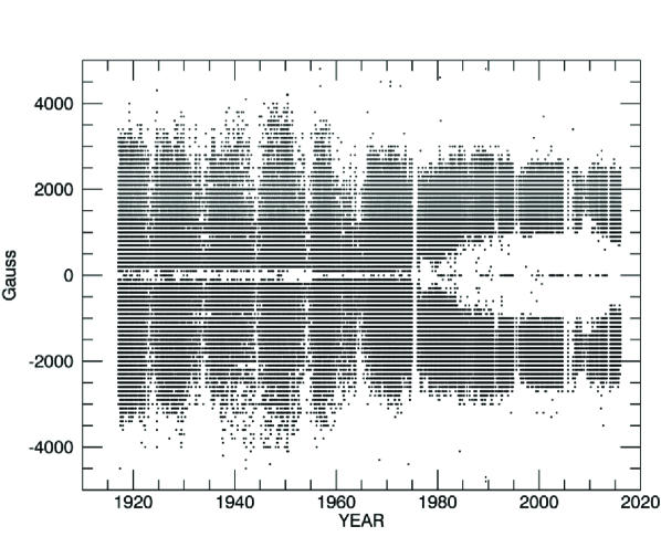
Figure 3: Field strengths (dots) measured in all sunspots included in our digitization project.

The data extracted from the drawings were placed in a fully searchable database based on an open-source relational database management system MySQL. Each drawing is represented by a set of the following parameters: date and time of observations (both local and UT), atmospheric seeing, observer’s initials, observer’s notes, radius of solar disk in pixels, the image x,y coordinates of the center of the solar disk in pixels, P angle (orientation of the solar north relative to terrestrial north direction, degrees), B angle (the latitude of the center of solar disk, degrees), Carrington longitude of the solar central meridian (degrees), number of sunspots on a drawing, and the extracted (or expected to be extracted) data for each sunspot as listed in Table 4. The database is expandable to include other parameters (e.g., MWO or NOAA group number) or a similar type of data from other instruments. Figure 3 shows the field strengths of all measured sunspots.

4 Known issues with measurements

The final database has several deficiencies of different origins. Thus, for example, we can see an upper limit in the field strengths measured after 1961 (following the switch to spectral line Fe I 525.0217 nm; see Section 2). A slightly lower upper limit can be identified in post-1994 data. According to the lookup Table 2, there should be no measurements of field strengths above 2600 G after 1994. However, the drawings taken during this period show field strengths of 2700 G. Based on communication with the current observer (Steve Padilla), the largest sunspots may show field strengths, which appear to be outside of the measuring range (60$\degr$ of tip plate). For these sunspots, the field strength is recorded as 2700 G. A few data points in post-1994 data, which show even larger field strengths in Figure 3, are due to digitization errors.

Another prominent feature is the absence of weak field measurements in the later part of the dataset. Prior to mid-1970, it was not uncommon for the observer to measure sunspot field strengths as low as 100 G. Between 1975 and 1985, the data show a clear trend with fewer weak field measurements then in previous years. According to Larry Webster, the head observer at that time, “this trend is associated with two big changes related to replacing the Babcock grating [no. 7, Table 1] by Bausch and Laumb grating [no. 8, Table 1] following the pit flood and the restoration of the original 8-inch Littrow lens. These two changes produced a significant improvement in the quality of the spectrum at the final eyepiece and, as the result, [he noticed that] all spots that could be resolved on days of good seeing showed fields of 1500 G or more. It took a while for all the observers to have enough good seeing experience that they agreed [with him], so there was not a jump [but a gradual change] in the minimum field immediately following the two above upgrades.” We note, however, that the trend of fewer weak field sunspot measurements starts in about 1976 – well before replacing the grating no. 8 (1982, Table 1). Interestingly enough, the observations of sunspot field strengths taken at the CrAO (Pevtsov et al. 2011, and references therein) also show a development of a similar gap in weak fields. Unlike the MWO observations, however, the gap in CrAO data already appeared in about 1965-66 and, by early 1970s, the measurements of fields less than 1000 G became extremely rare. By contrast, sunspot field strength measurements from the Main (Pulkovo) Astronomical Observatory (Pevtsov et al. 2011, and references therein) exhibited a gap in field strengths since the beginning of that dataset (1957). This gap (or minimum) in weak field strength measurements, which is subjective, may demonstrate the impact of a somewhat new knowledge (e.g., expectations from theoretical studies) on measurements, when the observer consciously tries making the observations to fit his or her understanding of a physical phenomenon (i.e., no sunspots should have a field strength smaller than 1000–1500 G).

Figure 3 also shows the presence of a slight observational (quantization) bias in the measured field strengths. This bias can be identified by following one of the horizontal streaks in Figure 3. Thus, for example, the density of points at 2000 G is higher than the density of measurements in two neighboring streaks (1900 and 2100 G). This bias further reveals itself in a histogram of field strengths (not shown) as small local peaks in the number of measurements at (both positive and negative) 800, 1000, 1500, 1800, 2000, and 2200 G. In bins neighboring these values (i.e., 900, 1100, 1400, 1600, 1700, 1900, and 2100 G), the number of measurements is lower. The origin of this bias is unknown, but we might speculate that it could be due to a subjective preference, when the observer rounded up the measured tip angle to the “nearest” integer angle. This bias is present in both 1917-1960 and 1961-2016 subsets of data, but it is stronger in the former.

Hale & Nicholson (1938) indicated that only measurements above 1000 G are reliable. Livingston et al. (2006) also noted that the measurements of magnetic field strengths weaker than 1000 G are unreliable because in the weaker fields the Zeeman splitting for Fe I 6173.343 Å becomes comparable to the Doppler width of the spectral line. On the other hand, the same article (Livingston et al. 2006) countered this by a statement that a well-trained observer can consistently measure fields weaker than 1000 G, and by providing an example, where multiple measurements by the same MWO observer agree within 100 G.

While we tend to agree that the measurements of B$\la$ 500-1000 G should be treated with a caution, the polarity measurements appear to be very robust. In a few selected cases, we checked the polarity of features with weak magnetic field during their disk passage, but we did not find a random reversal of polarity, which should have occurred if those field strengths were unreliable (i.e., below a detection threshold). Nevertheless, in our analysis of drawings, we came across with a very small number of erroneous polarity measurements when the polarity of a same sunspot changed as it crossed the solar disk.

5 Errors and uncertainties from digitization

When the original drawings were scanned by the observer at MWO, the scanning area was deliberately reduced by cutting off what the scanner operator considered as unessential information. Thus, for example, the scanned area often stops exactly at the limbs (and sometimes, limbs near the equator were excluded). In some cases, the scanned images may exclude one of the solar limbs altogether; this is probably because no sunspots were present in that part of the Sun. These omissions make it harder to establish a proper orientation of drawings with respect to their E-W orientation. The omissions may also lead to larger uncertainties in fitting the solar limb. The scanned images from 1996 till early 2000 do not include the date and time of observations. The latter omission hinders the proper calculations of the Carrington longitude. The original drawings contain information on the sequential number of each drawing, the number of groups, and (sometimes) the number of sunspots. There is also information on the orientation of the drawing (angle) relative to the direction of the solar equator. Unfortunately, this information was excluded from the scanned area. One of the coauthors (AAP-2) visited the archives of Carnegie Observatories in summer 2018 and photographed the drawings of 1996-2000 that miss this metadata. These photographs are used to update the MySQL database with the correct metadata, although this update has not been completed yet. Our visit to the archive of Carnegie Observatories uncovered that images of scanned drawings available online may be different from the drawings preserved in the archive. Some of these discrepancies could be explained by the processing of drawings at MWO, which involved several steps as follows:

1. The spots are drawn using the projected solar image as a guide.

2. The drift angle is measured by offsetting the image in an EW direction. The date and time were then entered to calculate the p angle.

3. The polarities and field strength are measured with the tipping plate.

4. The group type is identified from the distribution of the polarities and configuration of the spot parts.

5. The center of gravity as judged by the observer is identified and noted by vertical and horizontal tic marks.

6. The positions of the spot groups are determined from the Stonyhurst charts and noted on the drawing.

7. The observation time is entered on the drawing along with the observers ID, observing conditions, and any other comments. The intent was to record the mid-point of the drawing process but because the time had been entered to get the drift angle that time was occasionally used.

8. After 1996 the drawing was scanned and posted to the web page.

9. At the end of the month the drawings for the month were reviewed by one of the senior observers, obvious errors were corrected, either erased or crossed out. Typically these errors are of a typographic nature.

10. The final parameters of each spot group were entered into the monthly sunspot report and the actual drawings were stored in the archive of the Carnegie Observatories in Pasadena. The final parameters are online at the MWO web page and they are also available from Solar Geophysical Data (SGD) . These reports are available for the years between 1962 and 2004.

Between 1996 and early 2000 the scanner in use for the promptly posted drawings was too small, resulting in the loss of critical metadata on these posted images. This metadata (time and date of observations) is available from the SGD reports and the entries in that publication are definitive. Copies of spots that were outside the scanned area were digitally relocated to the page area and labeled as an inset. The relocated tic marks and Stoneyhurst positions are from the actual locations in such cases. Examples of such insets can found in 15 May 1999 and 29 August 1999 scanned drawings. Owing to the review process, we caution that there may be differences between the posted images and the definitive publication.

Since the digitization of the drawings was done using manual identification, there could be misidentifications and some features could be completely missed. In addition, there are errors that were made when the information from the drawings was entered manually during the digitization process. This includes errors in the time of observations, sunspot polarity, and field strength. We evaluate the level of errors using entries by two students. The students processed over 28,000 images spanning 1917 through 2017. Their task was to enter the metadata (date and time of observations, coordinates of numbered groups identified on drawings, seeing, and comments). In an effort to expedite the work the students were assigned either odd or even years. As a benchmark of the quality of their work, both students processed the same drawings for years 1920, 1940, 1960, 1980, and 2000. Examining these overlapping years allows us to understand the level of possible human errors. The first error arises in the number of images processed. There were 1493 images spanning these five overlapping years. One student processed all images while the other only processed 1481, thus missing 12 images or about 0.8% of images in this sample. Of the 1481 images that they both processed there were 51 differences in hour, minute, time designation (AM, PM, or UT), or seeing on 35 images, which is an error rate of 0.86% limited to approximately of 2.3% drawings. These errors included those that were caused by poor handwriting, multiple observation times, and seeing values shown on the drawings, swapping hours and minutes and errors with no identifiable reason. The analysis of errors indicates that the quality of manual digitization improved as students gain the experience working with the data. Noticeably, fewer mistakes were made in relation to multiple and missing entries for time and seeing conditions. This could also be attributed to better policies being adopted with regard to the information being recorded on the drawings. Handwriting varies wildly between the observers and definitely affects the amount of mistakes. Knowing the observers, it might be possible to identify those observers whose drawings have a higher risk for mistakes during the process. A bigger problem is the amount of unforced errors, for example, errors with no noticeable cause, especially during the later overlapping years (1980 and 2000).

From the analysis of “number of errors by year”, the big worry is the number of unforced errors (unknown cause), which include omitted or incorrect times (hours, minutes, seconds, AM/PM/UT designation) and seeing quality. However, overall the data quality improved with considerably fewer errors recorded from 1960 onward. From the analysis of “type of errors”, most errors occurred only once except for errors with no obvious (unknown) cause and poor handwriting. There is a marked difference in that one of the students made many more of these unforced errors. Breaking down the errors by year, we can see that one student was fairly consistent with unforced errors, committing at least one error in every year except for 1960. In contrast, the other student committed all of his unforced errors on 1980 data.

Assuming that quality of the data and the error rate remained consistent across the entire dataset we would expect to see a total of 884 drawings with at least one error, of which 249 are due to an error introduced by the human mistake, such as swapping hours and minutes or other error (unknown cause). Owing to early oversight, the length of the comment field was limited to 100 characters, which in some cases had truncated a long comment.

The criteria for the digitization program had evolved as the project developed. In the early period of the project, sunspots without the field strength measurement (marked only by a letter corresponding to their polarity) were not included in the digitized database. Later, these sunspots were added, but to accommodate the input format, the operator would have to assign either $+$49 or $-$49 (the maximum field strength allowed by the Kislovodsk digitization program). The database contains about 6.3% of entries with $\pm$4900 G. While majority of these entries correspond to sunspots with only polarity (no field strength) measurement, there could be a few sunspots whose field strength was that value. Future updates will correct this uncertainty.

Digitization made by the NSO team saved the image coordinates of all features (the disk center, limb marks, and sunspot locations), but the digitization made by the Kislovodsk team only stored image coordinates for the disk center. For other features, only the heliographic coordinates were preserved. The image coordinates could be useful in case the heliographic coordinates need to be updated. The image coordinates could be computed using the heliographic coordinates of sunspots, but the conversion depends on scaling of the scanned images. Unfortunately, after the digitization was completed it was discovered that some original images stored on MWO server had been modified by adding comments to the digital images. This changed the size of images and inadvertently broke the scaling between the image and heliographic coordinates. Future users of this dataset may notice such cases when the recomputed image coordinates of marked features (e.g., sunspots) may be offset relative to the features on a drawing.

In summer 2018, one of the coauthors (AAP-2) examined the original drawings held in the archive of the Carnegie Observatories and discovered several drawings (from 1996–2000 period), which were not scanned. Thus, these data are absent from the digitized dataset. It is currently unclear how many drawings were not scanned, but we do not expect it to be a large number.

These deficiencies will be addressed in the later editions of the dataset, subject to available resources. To keep track of future modifications to the original digitized dataset, we introduce the version number. The results of the initial digitization already published in some early papers (e.g., Tlatova et al. 2015, 2018) are designated as version MWO_SPOTS_20171101, where the numbers represent the year, month, and day of last changes to the dataset. The current version of the dataset described in this paper is MWO_SPOTS_20180801.

Uncertainties in the heliographic coordinates of sunspots may arise from an incorrect determination of image coordinates of the solar features, position of the solar disk center, and radius of the solar disk on drawings. As one example of an observer error, the first drawing (4 January 1917; see online archive of sunspot drawings at ftp://howard.astro.ucla.edu/pub/obs/drawings), the CMD of the leading sunspot of the Mount Wilson group 516 is denoted as 9W, while in fact, the correct CMD should be 19W.

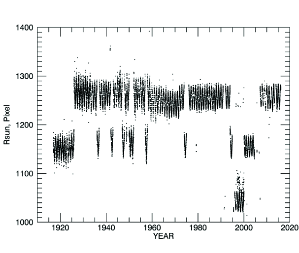
Figure 5: Radius of the solar disk for all dataset as measured from drawings.

One source of uncertainty can be associated with the thickness of lines drawn by the observer. Limited examination of drawings for different years indicates that a typical thickness of lines varies between 5 and 7 pixels (in scanned image scale). For comparison, a typical radius of the solar image is about 1250 pixels. Figure 4 provides an example of variations in radius of the solar disk (R_sun) as measured from the drawings. As expected, R_sun shows an annual variations of about $\pm$1.6%. Amplitude of R_sun in pixels depends on scaling that was selected during the image scanning. We note a deviation between the fitted sine curve and the measured R_sun in mid-1982, which has been traced to a use of slightly different resolution for a flatbed scanner. A significant deviation in early 1979 (vertical line reaching very low values of R_sun) is also due to a significantly different scanner scale selected by the observer. Smaller spikes in R_sun are random uncertainties in the radius of the circle fitted to the solar disk. The deviations of the measured R_sun from the fitted sine curve are normally distributed and have a zero mean and standard deviation of $\sigma$ = 4.5 pixels. The nonuniformity in selected scaling for scanning the drawings can be clearly seen in Figure 5. Uncertainties in solar latitude and CMD of sunspots arising from effect of the above uncertainty in R_sun on image-to-heliographic coordinate transformation vary with heliographic distance from the solar disk center. For heliocentric distances $\rho\leq$ 70$\degr$ the uncertainty is smaller than 0.10 degrees. For $\rho\approx$ 75$\degr$ the uncertainty reaches 0.15 degrees. At $\rho\approx$ 85$\degr$ the uncertainty is about 0.5 degrees, and near the limb ($\rho\approx$ 87$\degr$), it increases to more than one degree. The above uncertainties correspond to one standard deviation derived from 1000 realizations of coordinate transformations using six-pixel uncertainty in the position of the solar limb.

The drawings do not include northern or southern parts of the solar disk at high latitudes and, thus when determining the radius of the solar disk, only eastern and western limbs were used. This might introduce a minor uncertainty due to a distortion of the (assumed round) shape of the solar disk by atmospheric refraction. However, for a reasonable zenith angles, the effect is small (less than 1 arcsecond), when compared with the average angular diameter of solar disk of about 1800 arcseconds (see Figure 4 in Corbard et al. 2013). Even a larger uncertainty in solar limb could result from the atmospheric seeing. However, a typical daytime atmospheric seeing at MWO is about 2-3 arcseconds, which approximately corresponds to 3-4 pixels on a typical drawing. Thus, the overall effect from both atmospheric refraction and atmospheric seeing is comparable to the uncertainty associated with the line thickness of drawings.

Uncertainties in the heliographic coordinates of sunspots may also arise from a slight displacement of sunspots during the time period when the observer records sunspots on a drawing. During this time, the spots may change their positions because of solar rotation, which could add as much as 0.15 degrees of uncertainty to their observed longitudes (assuming that it takes 15 minutes to complete the drawing). The 3 arcsecond atmospheric seeing could result in $\approx$ 0.18 degree uncertainty in measured position of a sunspot. Based on the above arguments, we conclude that with the exception of errors in identifying sunspots, the uncertainties in the heliographic coordinates do not exceed 0.5 degrees.

6 Comparison with other datasets

To compare the sunspot field measurements from different instruments, we selected 100 sunspots observed over the 20-year period between 1994 and 2014 both at MWO and CrAO. Sunspots that were observed on the same day by both observatories were selected for comparison. To ensure that the same magnetic features were compared, we excluded sunspots with multiple umbrae or a complex magnetic pattern. The sunspots were also selected to represent a broad range of field strengths.

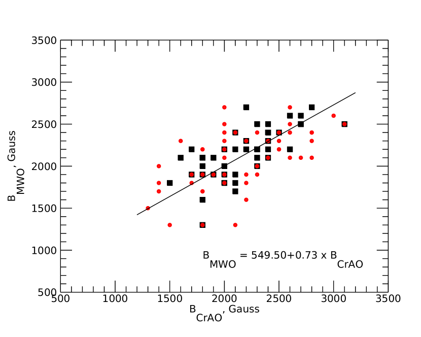
Figure 6: Comparison of same-day measurements of field strengths of 100 sunspots observed at MWO and CrAO. Observations from 1994–2003 are shown by black squares, and data for 2004–2014 are shown as filled red circles. The solid line indicates the least-squares fit by the first degree polynomial with errors in both MWO and CrAO data. The coefficients of best-fit line for all data are shown in low-right side of the Figure.

The program of measuring sunspot field strengths at Crimea started in mid-1950s and (with some brief interruptions) has continued until the present (Pevtsov et al. 2011). The measurements are made visually by several staff observers, which is the same practice as in past MWO observations; more recent observations at MWO are taken by a single observer. Additional information about the quality of CrAO sunspot field strength measurements can be found in Lozitska et al. (2015). In a search for possible systematic trends, we divided the dataset in two equal halves: 50 sunspots observed during 1994–2003 and 50 sunspots in 2004–2014. Figure 6 shows a scatter plot of measurements from one observatory versus the other. The measurements from the two observatories correlate reasonably well, Spearman rank correlation coefficient is 0.64 with (probability of no correlation) $p$ = 6 $\times$ 10^-13. The local time difference between the two observatories is ten hours, which may partially explain the scatter between the measurements of the same sunspots in two observatories. The least-squares linear fit (assuming 100 G uncertainties in both MWO and CrAO measurements) yields B_MWO = (549.00$\pm$82.23) + (0.73$\pm$0.04) B_CrAO (see Nagovitsyn et al. 2016, for a discussion of the fitting approach). Slope of fitted line is steeper for the early period (1994–2003), B_MWO = (436.45$\pm$134.84) + (0.79$\pm$0.06) B_CrAO than for the (later 2004-2014), B_MWO = (646.88$\pm$102.30) + (0.67$\pm$0.05) B_CrAO.

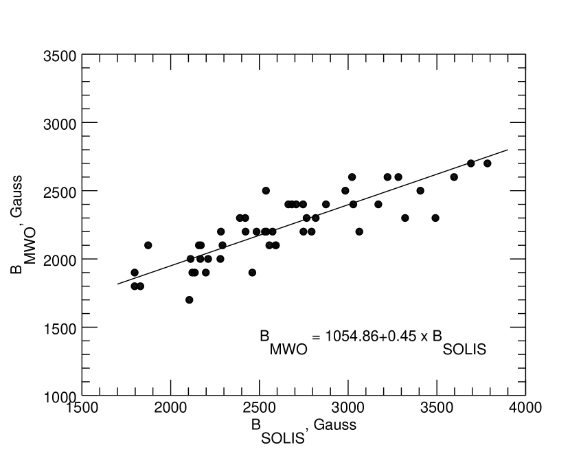
Figure 7: Comparison of field strengths of 50 sunspots observed at MWO and by VSM/SOLIS (Zeemanfit code). Solid line is a least-squares fit to the data by a first degree polynomial. Parameters of fitted polynomial are shown in the lower part of the plot.

For another comparison, we used the total field strengths derived by fitting the Stokes I profiles observed by the Vector Stokes Magnetograph (VSM) on Synoptic Optical Long-term Investigation of the Sun (SOLIS) platform (e.g., Balasubramaniam & Pevtsov 2011). We carried out the fitting via the SOLIS Zeemanfit code (Hughes et al. 2013), which employs a three-component fit to the non-polarized (Stokes I) profile of Fe I 6302.5 Å spectral line. In sunspots with a strong magnetic field, the Zeeman splitting becomes wide enough for the triplet nature of the line to be clearly visible in non-polarized light (for example, see Figure 1a). Therefore, a three-line fit to the spectra provides a fairly robust measure of the total magnetic field strength. The field strengths using Zeemanfit are computed routinely beginning in late-2013. Figure 7 shows a scatter plot of MWO sunspot field strength measurements versus SOLIS Zeemanfit for 50 sunspots observed between October 2013 and December 2014. For this comparison, sunspots were selected on the basis of closeness in observing time between the two instruments and to ensure a broad range of field strengths in a sample. As it is difficult to identify the exact location of a flux element for which the MWO measurements were taken, for this comparison we avoided sunspots with complex polarity patterns to minimize spatial misidentification of measured flux elements. Two data sets show a good relationship with Spearman rank correlation $r$=0.85 and $p$= 5.6 $\times$ 10^-15. The least-squares linear fit returns B_MWO = (1054.86$\pm$89.81)+(0.45$\pm$0.03) B_SOLIS. For this fit, we assumed the uncertainty in B_MWO measurements to be 100 G. For SOLIS data, the uncertainties are returned by the Zeemanfit code, which for this subset of data were between 47 G and 251 G. In this comparison, we took the MWO field strengths as they are shown on the drawings without any correction for a nonlinearity in the measured fields.

In absence of evolution, the magnetic field strength in a stable sunspot should exhibit very limited center-to-limb variation. As a test, we selected several well-developed sunspots and followed the variations in measured field strength during their disk passage. As a general rule, the field strength exhibits clear maximum when the sunspot is near the central meridian. In all studied cases, the decrease in observed field strength as function of the heliographic distance from solar disk center is less steep as compared with the cosine function. On average, a difference between sunspot field strength near the central meridian and the heliocentric distance of 50$\degr$ is about 300 G, which is in agreement with the center-to-limb variation in the height formation of the photospheric spectral lines and known vertical gradient of the magnetic field in the photosphere (Borrero & Ichimoto 2011, 1 G/km,).

7 Conclusions

The results reported in this article concern the digitization of historical sunspot field (strength and polarity) measurements made at MWO. The systematic observations began in 1917 and have continued until the present with a few brief interruptions. These manual measurements represent the earliest observations of the magnetic fields on the Sun and, while they may have many shortcomings when compared with the modern polarimetric observations, these data provide a critical link with past magnetic activity of the Sun. Given the long-term duration of this time series, we think that its continuation would be extremely important. Based on comparison with CrAO and SOLIS/Zeemanfit measurements, we argue that the time series could be successfully continued using the data from these two observatories in case the sunspot operations at MWO should end.

The digitized dataset may still contain some errors related to the orientation of drawings or to an incorrect identification of solar limbs and/or sunspot features. There could also be a few errors related to the time of observations. These errors will be corrected in future releases of the dataset, once the team becomes aware of the specific errors.

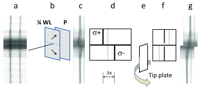
Figure 1: Principle of measuring the field strength in sunspots. (a) Example of Zeeman splitting of spectral lines Fe I 6301.5 Å (left) and Fe I 6302.5 Å (right) as observed by the spectropolarimeter on board the Hinode spacecraft. The horizontal direction corresponds to the wavelength space and the vertical direction shows spatial dimension (along the spectrograph slit; in this example, across a small sunspot). The dark diffuse horizontal band in the middle of the spectra corresponds to sunspot umbra, and two gray bands above and below this dark band are sunspot penumbra. Brighter areas farther outward from the penumbra correspond to the photosphere. There, the brighter and darker horizontal lines in panel (a) correspond to the granulation pattern as the spectrograph slit crosses (brighter) centers of granules and (darker) intergranular spaces. Owing to the atmospheric seeing, the granulation pattern is less visible in spectra taken with VSM/SOLIS (panels c and g). To measure the magnetic field, two Zeeman components with left- and right-hand polarization are spatially separated with the two strips of optical retarder (quarter- wavelength plate, 1/4 WL) and a polarizer (P). Upper and lower strips of retarder are oriented orthogonal to each other and at 45 degrees to the polarizer, as shown in panel (b). Each strip (retarder and polarizer) transmits only one of two Zeeman components, which allows the left-hand and right-hand polarized components been separated in the vertical direction (panel c). Panel d is a simplified, schematic representation of panel c (central $\pi$ component is shown as a dashed line). The value $\Delta x$ is a distance between two $\sigma$ components, which needs to be measured to determine the field strength. By rotating a tip plate (panel e), the observer brings two oppositely polarized components in line with each other (panels f and g), and the tip angle is used to derive the field strength.

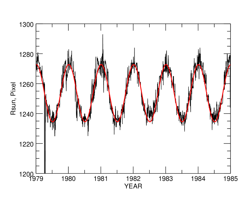
Figure 4: Radius of the solar disk in 1979–1982 as measured from drawings (black solid line). Red line shows the best least-squares fit by a sine function.

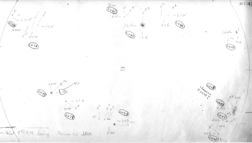
Figure 8: Example of drawing taken on 16 January 1926. Sunspot outlines lack fine details. Scanned image excludes portion of the drawing with year and month of observations and part of solar limb.

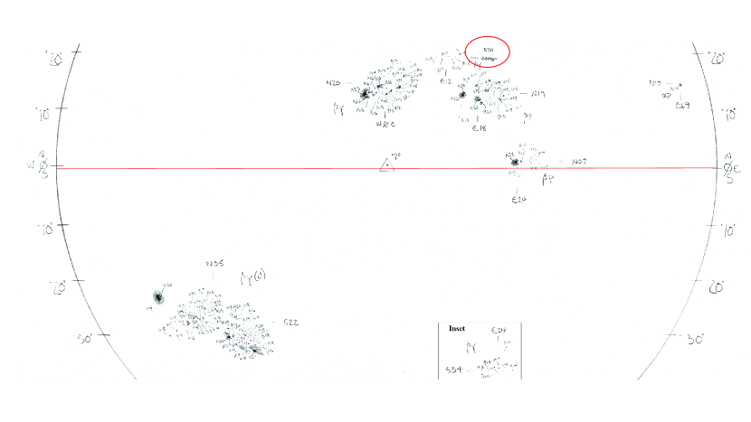
Figure 9: Example of drawing taken on 29 August 1999 showing high degree of detail. The scanned image excludes portion of the drawing with information about date and time of observations. The red line shows the horizontal direction in image orientation. Comparing the location of end points, it is clear that there is a slight misalignment between the horizontal direction and east-west orientation. Portion of the image enclosed by box is an inset, which shows portion of solar image not in its correct location on solar disk. The red oval indicates an example of an error in the heliographic coordinates of an active region. In this particular case, the later correction of latitude of this region is in error; compare the number with the approximate latitudes indicated on the solar limbs.

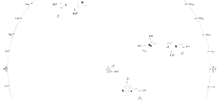
Figure 10: Example of drawing taken during the period of a poor seeing. The location of solar limb is shown approximately, using ”wavy” lines.

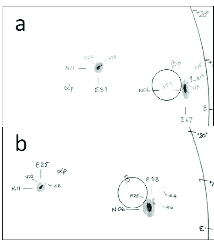
Figure 11: Example of incorrect measurement of sunspot polarity. Polarity of a sunspot observed on 13 November 2013 (panel a) was determined as ”V” (negative), but on all following days (panel b, 14 November 2013), the measured polarity was ”R” (positive). The circles indicate the polarity measurement for this sunspot.

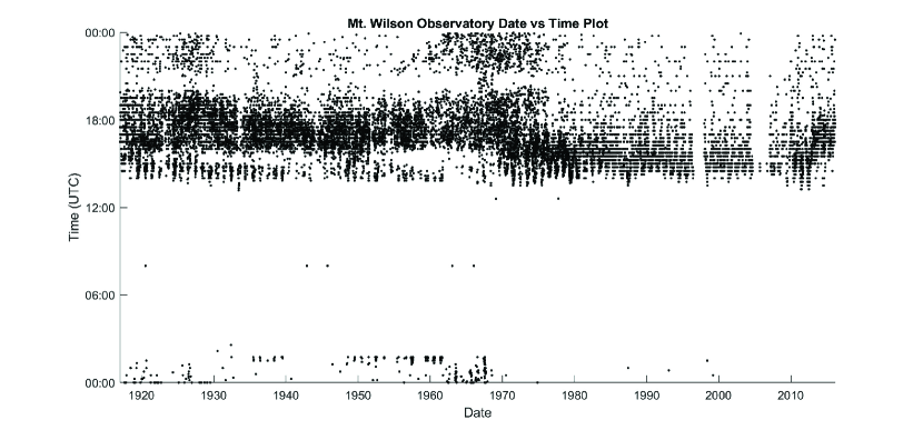
Figure 12: Universal time of observations for all drawings in the dataset. The vertical gap in 1996-1997 corresponds to period when the time of observations was not included in the scanned images. These data will be updated in later versions of the dataset. A second vertical gap corresponds to 2004–2007, when the sunspot drawings program was shut down. Annual variations in the earliest time of observation are due to change in the sunrise time during the year. Two horizontal gaps in seeing in the time of observations correspond to a shading of the coelostat mirror tracking the Sun by the support pillar and secondary mirror (which reflects light to the main telescope mirror) in early morning hours (about 15:00 UT) and the break for the lunch hour at the MWO (about 20:00 UT). The lunch break was a formal event at MWO until about 1984, when the operations of solar telescopes were transferred from Carnegie observatories to UCLA. Early morning horizontal gap (15:00 UT) seems to disappear after 1970, which suggests that at that time, the morning observations may have been taken with the first flat mirror moved to the east position, and thus having a strongly oblique angle between the two mirrors.

Table 1: Parameters of spectrograph gratings used during the lifetime of project

No.	Start date	grooves	$\lambda$	$m$	$s^{-1}$	Scale	Measured and true field strengths (G)
		mm-1	Å		mm/Å	100 G	100	1000	2000	3000	4000
1	1917	602	6173	2	2.97	1$\degr$	90	920	1900	3010	4320
2	1930	602	6173	2	2.97	1$\degr$	90	920	1900	3010	4320
3	May 1949	400	6173	3	2.96	1$\degr$	90	920	1900	3020	4340
4	29 Sep 1950	400	6173	3	2.96	1$\degr$	90	920	1900	3020	4340
5	19 May 1955	600	6173	2	2.96	1$\degr$	90	920	1900	3020	4340
6	22 Aug 1960	600	6173	2	2.96	1$\degr$	90	920	1900	3020	4340
same	Oct 1961	600	5250	5	11.15	0.5$\degr$	90	940	2180	4050	…
7	24 Dec 1962	610	5250	5	11.66	0.5$\degr$	90	900	2080	3870	…
8	17 May 1982	632	5250	5	12.96	0.5$\degr$	80	810	1870	3480	…
9	21 Nov 1994	367.5	5250	9	15.27	Table 2	…	760-800	1880-1940	…	…

Table 2: Conversion table used by the observer for measurements taken after 1994.

Tip angle	Measured	True
deg.	field, G	field, G
22-23	1000	800
24-26	1100	800-900
27-28	1200	1000
29-30	1300	1100
31-32	1400	1100-1200
33-35	1500	1200-1300
36-37	1600	1400
38-39	1700	1500
40-42	1800	1600-1700
43-44	1900	1800
45-46	2000	1900
47-48	2100	2000-2100
49-51	2200	2100-2300
52-53	2300	2300-2400
54-55	2400	2500-2600
56-57	2500	2700
58-60	2600	2800-3000

Table 3: Historical periods when the DST was in effect in Los Angeles, California (years after MWO adopted the UT timing practice are not included)

Years	Start date	End date	Note
1918-1919	31 Mar	27 Oct	Introduced by “Standard Time Act of March 19, 1918”
			abolished by 66th U.S. Congress in ”CHAP. 51.
			An Act for the repeal of the daylight-saving law”
1942-1945	9 Feb 1942	30 Sep 1945	year-round DST by Public Law 403 ”Daylight Savings Time”
1949-1966	last Sunday in Apr	last Sunday in Sep	DAYLIGHT SAVING TIME California Proposition 12 (1949)
1967-1972	last Sunday in Apr	last Sunday in Oct	U.S. Uniform Time Act of 1966

Table 4: Example of entries reserved for parameters extracted from the drawings

No.	Parameter description
1	latitude of sunspot, degrees
2	CMD of sunspot, or “longitude” relative to central meridian, negative/positive
	east/west of central meridian, degrees.
3	longitude (Carrington longitude of sunspot, degrees
4	heliocentric distance, r/R, where r – distance from disc center, R – radius of solar disk
5	Reserved for: area of sunspot, millionths of solar hemisphere
6	Reserved for: area of sunspot, pixels
7	Reserved for: size of sunspot in latitudinal direction, degrees (could be negative as it is computed as difference in latitudes).
8	Reserved for: size of sunspot in longitudinal direction, degrees
9	Reserved for: average intensity
10	Reserved for: contrast of sunspot relative to surrounding photosphere
11	Reserved for: minimum intensity in sunspot
12	Reserved for: maximum intensity
13	Reserved for: tilt angle relative to equator, degrees
14	field strength (in units of 100 G)
15	Reserved for: length of outer boundary of sunspot, pixels

Appendix A Example of uncertainties arising from quality of hand drawings

Uncertainties in heliographic coordinate transformation may arise from several sources including uncertainties in fitting solar limb, image position of sunspots, orientation of scanned image, and uncertainty in time when the position of a specific sunspot was recorded.

When the modern observations of sunspot drawings are taken, the observer orients the drawing paper in the direction parallel to solar equator (see, Section 5). This is done manually by eye under variable atmospheric seeing conditions, and thus inherently, the image orientation must have some uncertainty. The exact amplitude of this uncertainty depends on the observer’s level of training and the observing conditions, but it is reasonable to assume that it should not exceed about one degree (larger image inclinations are usually detectable by eye). This error mainly affects the heliographic latitude, and it increases with the distance from the disk center. For each individual observation, the error is systematic, which means that the latitudes of sunspots located near one solar limb are slightly larger than the true latitude, while the latitudes of sunspots located near opposite limb are slightly smaller. It might be possible to estimate (and correct) this error in orientation of daily images, by comparing the latitudes of sunspots in sequential daily observations assuming that sunspot latitude does not change as it crosses solar visible disk. Alternatively, we can estimate the error in heliographic coordinates for each sunspot location on the disk using, for example, Monte Carlo simulations. Based on the above considerations, the sunspots situated at the solar limb should have an uncertainty in their latitude of about one degree or less. For sunspots near the disk center the uncertainty in latitude is much smaller.

The image orientation could have been further altered during the drawings scanning (i.e., placing the drawing slightly tilted relative to scanner bed). This error in image orientation could be readily detected (and corrected) if the scanned image includes both solar limbs with markings corresponding to location of solar equator (see, Figure 9). Unfortunately, number of scanned images may exclude either one of the limbs or its near equatorial part (Figure 8). In the latter case, the errors in heliographic coordinates can be evaluated on the basis of Monte Carlo simulations assuming some mean value of tilt of images based on other scanned images.

In the worse case scenario, two errors (errors in orientation due to observing conditions and due to image scanning) could combine, thus doubling the uncertainties in latitude of sunspots close to solar limbs.

The above procedure of orienting the drawing paper in respect to solar equator was not always followed, and thus there are several cases in early part of the dataset when the drawings do not have a proper orientation (e.g., drawing orientation was not corrected for P angle). While we tried determining the proper image orientation for such cases, there could be some instances that were not corrected. Those should become evident when the derived parameters of sunspots are used to investigate their evolution during solar disk passage with following visual inspection of individual images. Once detected, such cases should be used to update the database.

Uncertainties due to unknown time of observations have a larger effect on the heliographic longitudes. Usually, the time recorded on the drawing corresponds to the beginning of observations although in some cases the drawing may show a time range (beginning and end time of drawing). Based on more recent observations, typically the time to complete a drawing may vary between 15 and 30 minutes although it may take longer depending on the level of observer’s training, atmospheric conditions, and sunspot activity; for example, we compare the number of features marked by the observer on drawings shown in Figures 8 and 9. Based on the initials of the observers, in early part of the dataset, it was not uncommon to have an observer taking observations only for one or two years and using substitute observers (nonsolar members of MWO scientific and supporting staff, and even observatory visitors). Thus, it is very possible that some drawings taken in early period of the dataset could take longer than 30 minutes. Figure 12 shows UT time of drawings for 1917–2016 period. After about 1979, the time shows quantization, when the observers started rounding up the time to the nearest 15 minutes. Similar quantization could also be seeing in some early periods although it is not as pronounced as in post-1979 period. Time quantization may create a visual impression of fewer observations taken after 1979. This impression is incorrect. The number of observations per year is about the same during these two periods.

During 1967-68, there are larger uncertainties in the time of observations. It appears that more drawings did not show “PM” or “AM” designation, and some observers may have been experimenting with using UT time. The time of observations for this period may require additional examination.

Within the period each drawing was taken, it is unknown which sunspot was drawn at what time. This uncertainty in time of drawing for each feature introduces uncertainty in their heliographic longitude. Owing to solar rotation, in half an hour the sunspot location could change by about 0.3$\degr$ depending on sunspot latitude. Figure 12 shows that for several drawings the time of observations converted to UT may be incorrect. In rare cases, the drawings were taken late in the day when the UT time may exceed 24:00. This could result in an error in the day of observations; the day of observations is recorded as a calendar day, not UT day. This will be verified and corrected in future releases of the dataset. The uncertainty in time should be considered when the sunspots from this dataset are used for determination of solar rotation and sunspot proper motions.

At the beginning of the dataset, the drawings were considered as approximate sketches and did not contain fine details (Figure 8). Images taken in later periods show extremely high level of detail (see, Figure 9). This difference in degree of detailization may affect the uncertainties in image location of sunspots as well as their (sunspot) areas with higher uncertainties for more approximate images. The exact amplitude of these uncertanties may be hard to estimate, but as a low limit, we can assume that they should not be smaller than the thickness of a pencil used by the observer. Based on our analysis of width of solar limb on selected drawings, it is about 5–7 pixels in scanned images (see, Figure 4). This value can be used in combination with the size of sunspots and their location on the disk as well as the uncertainty in the location of fitted solar limb and radius of solar disk on a drawing to derive a more precise estimate of uncertanties in heliographic coordinates of each feature.

Some drawings may contain insets – a portion of solar image drawn not in its right location (see Figure 9). Typically, insets were created by the observer to accommodate high-latitude groups falling outside of drawing paper. Some insets were created during the scanning process, as a solution to a limited size of a scanner bed. The center of sunspot group in the inset is marked by the observer (or scanner operator), and to convert image coordinates to the heliographic coordinates, we have to use these heliographic coordinates first to convert image coordinate of the insert to its proper location on the drawing, and then convert new image coordinates to proper heliographic coordinates. Such a double coordinate transformation provides only approximate correction for foreshortening effects, and thus this transformation may introduce uncertainties in relative heliographic coordinates of sunspots shown in the inset. Moreover, the heliographic coordinates shown on insets are approximate (rounded to a closest degree), which further increases uncertainties of heliographic coordinates of features shown as insets. The amplitude of the effect depends on heliographic position of the inset, and thus needs to be evaluated separately for each sunspot in the inset. We expect, however, that the resulting errors will be smaller than the errors resulting from uncertainties in radius of solar disk (limb fitting) and image orientation.

The location of solar limb is marked by the observer as part of making a drawing. Fitting circle to the hand-drawn solar limbs results in additional uncertainty in solar radius. However, we find such uncertainty is comparable to a thickness of pencil lines. When the observations are taken in poor seeing conditions, the observer may indicate the location solar limb by a ”wavy” lines as shown in Figure 10. For such days, the user should expect to see larger errors in heliographic coordinates, but this needs to be evaluated using Monte Carlo simulations with larger uncertainties both in radius of solar image and the location of sunspots on images. For this modeling, the amplitude of wavy pattern could be used as a measure of uncertainties in solar disk radius and image position of sunspots.

Figures 8-9 show examples when some metadata (e.g., date and time of observations) could be excluded during the scanning of a drawing. Once identified, such cases should be used to update the database.

In some rare occasions, the measured polarity of sunspots could be in error. The exact number of such erroneous measurements is hard to estimate, as they require a detailed examination of sequential drawings. We identified only a very small number of such errors.

Overall, our assessment is that the uncertainties in radius of solar disk, image orientation, and time of observation are the largest source of uncertainties in the heliographic coordinates. In general, the uncertainty in coordinates of sunspots is within 1–2°.

The magnetic field measurements show several systematic effects, which may be impossible to fully account for. The minimum uncertainty of each measurement is 100 G, but for some measurements, the errors could be much larger.