Legendrian Hopf links

Abstract.

We completely classify Legendrian realisations of the Hopf link, up to coarse equivalence, in the $3$-sphere with any contact structure.

1. Introduction

When we speak of a Hopf link in this paper, we shall always mean an ordered link $K_{0}\sqcup K_{1}$ in the $3$-sphere $S^{3}$, made up of oriented unknots forming a positive Hopf link, that is, $K_{1}$ is isotopic in $S^{3}\setminus K_{0}$ to a positive meridian of $K_{0}$. Two Legendrian realisations $L_{0}\sqcup L_{1}$ and $L_{0}^{\prime}\sqcup L_{1}^{\prime}$ of this Hopf link in some contact structure $\xi$ on $S^{3}$ are called coarsely equivalent if there is a contactomorphism of $(S^{3},\xi)$ that sends $L_{0}\sqcup L_{1}$ to $L_{0}^{\prime}\sqcup L_{1}^{\prime}$ as an ordered, oriented link.

The main result of this paper is the classification, up to coarse equivalence, of all Legendrian realisations of the Hopf link in $S^{3}$ with any contact structure.

For a brief introduction to the theory of Legendrian knots, i.e. knots tangent to a given contact structure, see [geig08, Chapter 3] or the beautiful survey by Etnyre [etny05]. The latter discusses the classification of Legendrian knots and covers a wide range of applications of Legendrian knot theory not only to contact geometry (e.g. surgery along Legendrian knots, invariants of contact structures), but also to general topology (e.g. plane curves, knot concordance, topological knot invariants).

Very little is known about the classification of Legendrian links (with more than one component). When Etnyre wrote his survey on Legendrian and transverse knots in 2005, the results about Legendrian links could be summarised on two pages. Since then, only a small number of classification statements on Legendrian links in the standard tight contact structure $\xi_{\mathrm{st}}$ on $S^{3}$ or in other tight contact $3$-manifolds have been added to the literature, e.g. [dige07, dige10]. The present paper goes considerably beyond those results, both concerning the range of Legendrian realisations covered by the classification and the variety of methods used in the proof. Our main theorem is the first complete Legendrian classification of a topological link type that includes Legendrian realisations in overtwisted contact structures.

Legendrian knots in overtwisted contact structures fall into two classes, loose and exceptional. The latter can be divided into two subclasses.

Definition 1.1.

A Legendrian knot $L$ in an overtwisted contact $3$-manifold $(M,\xi)$ is called exceptional if its complement $(M\setminus L,\xi|_{M\setminus L})$ is tight; the knot is called loose if the contact structure is still overtwisted when restricted to the knot complement.

An exceptional Legendrian knot is called strongly exceptional if the knot complement has zero Giroux torsion.

The notion of Giroux torsion and the related concept of twisting will be explained below. Previous classification results for exceptional Legendrian knots such as [geon] confined attention to strongly exceptional realisations. One of the reasons for this restriction is that classification results for tight contact structures on the relevant knot complement typically tend to require, as in [dlz13], that the Giroux torsion be zero. One of the significant features of our classification of Legendrian Hopf links, by contrast, is the fact that it includes Legendrian realisations where the link complement may contain torsion without being overtwisted.

Here is our main result. As mentioned before, $\xi_{\mathrm{st}}$ denotes the standard tight contact structure on $S^{3}$. Besides this standard structure, there is a countable family of overtwisted contact structures $\bigl{\{}\xi_{d}\colon\thinspace d\in\mathbb{Z}+\frac{1}{2}\bigr{\}}$, as we shall recall below. For the definition of the classical invariants $\mathtt{tb}$ (Thurston–Bennequin invariant) and $\mathtt{rot}$ (rotation number) of Legendrian knots, as well as other fundamentals of contact topology, the reader may refer to [geig08]. Our natural numbers $\mathbb{N}$ are the positive integers; $\mathbb{N}_{0}$ includes zero.

Theorem 1.2.

Up to coarse equivalence, the Legendrian realisations of the Hopf link are as follows. In all cases, the classical invariants determine the Legendrian realisation.

• In $(S^{3},\xi_{\mathrm{st}})$ there is a unique realisation for any combination of classical invariants $(\mathtt{tb},\mathtt{rot})=(\mathtt{t}_{i},\mathtt{r}_{i})$, $i=0,1$, in the range $\mathtt{t}_{0},\mathtt{t}_{1}<0$ and

  $$\mathtt{r}_{i}\in\{\mathtt{t}_{i}+1,\mathtt{t}_{i}+3,\ldots,-\mathtt{t}_{i}-3,-\mathtt{t}_{i}-1\}.$$

  For fixed values of $\mathtt{t}_{0},\mathtt{t}_{1}<0$ this gives a total of $\mathtt{t}_{0}\mathtt{t}_{1}$ realisations.

• For $\mathtt{t}_{0}<0$ and $\mathtt{t}_{1}>0$ the strongly exceptional realisations are as follows.

  • In $(S^{3},\xi_{1/2})$ there are realisations $L_{0}\sqcup L_{1}$ made up of an exceptional Legendrian unknot $L_{1}$ with invariants $(\mathtt{t}_{1},\mathtt{r}_{1})=(n+2,\pm(n+1))$, where $n\in\mathbb{N}_{0}$, and a loose Legendrian unknot $L_{0}$ whose Thurston–Bennequin invariant $\mathtt{t}_{0}$ can be any negative number, and $\mathtt{r}_{0}$ lies in the range

    $$\{\mathtt{t}_{0},\mathtt{t}_{0}+2,\ldots,\-\mathtt{t}_{0}-2,-\mathtt{t}_{0}\}.$$

    For a given $\mathtt{t}_{0}<0$, this gives us $2|\mathtt{t}_{0}-1|$ realisations.

  • In $(S^{3},\xi_{1/2})$ there are realisations $L_{0}\sqcup L_{1}$ consisting of the exceptional Legendrian unknot $L_{1}$ with invariants $(\mathtt{t}_{1},\mathtt{r}_{1})=(1,0)$ and a loose Legendrian unknot $L_{0}$, where $\mathtt{t}_{0}$ can be any negative number, and $\mathtt{r}_{0}$ lies in the range

    $$\{\mathtt{t}_{0}-1,\mathtt{t}_{0}+1,\ldots,\-\mathtt{t}_{0}-1,-\mathtt{t}_{0}+1\}.$$

    For a given $\mathtt{t}_{0}<0$, these are $|\mathtt{t}_{0}-2|$ realisations.

• For $\mathtt{t}_{0},\mathtt{t}_{1}>0$ the strongly exceptional realisations are as follows.

  • There is a unique realisation in $(S^{3},\xi_{1/2})$ with $(\mathtt{t}_{i},\mathtt{r}_{i})=(1,0)$, $i=0,1$. Both $L_{0}$ and $L_{1}$ are exceptional.

  • There is a pair of realisations with $(\mathtt{t}_{0},\mathtt{r}_{0})=(2,\pm 3)$ and $(\mathtt{t}_{1},\mathtt{r}_{1})=(1,\pm 2)$ in $(S^{3},\xi_{-1/2})$.

    There are three realisations with $\mathtt{t}_{0}=3$ and $\mathtt{t}_{1}=1$. Two of them with $(\mathtt{t}_{0},\mathtt{r}_{0})=(3,\pm 4)$ and $(\mathtt{t}_{1},\mathtt{r}_{1})=(1,\pm 2)$ live in $(S^{3},\xi_{-1/2})$; the third one with $(\mathtt{t}_{0},\mathtt{r}_{0})=(3,0)$ and $(\mathtt{t}_{1},\mathtt{r}_{1})=(1,0)$ can be found in $(S^{3},\xi_{3/2})$.

    There are four realisations with $\mathtt{t}_{0}=\mathtt{t}_{1}=2$: two with $\mathtt{r}_{1}=\mathtt{r}_{2}=\pm 3$ in $(S^{3},\xi_{-1/2})$, two with $\mathtt{r}_{0}=\mathtt{r}_{1}=\pm 1$ in $(S^{3},\xi_{3/2})$.

    In all cases, the individual link components are loose.

  • For any $\mathtt{t}_{0}\geq 4$ and $t_{1}=1$ there are four links realising these values of the Thurston–Bennequin invariants. For $\mathtt{t}_{0}\geq 3$ and $\mathtt{t}_{1}=2$ there are six realisations. The remaining invariants are listed in Table LABEL:table:se-invariants in Section LABEL:section:compute. The link components are loose.

  • For each choice of $\mathtt{t}_{0},\mathtt{t}_{1}\geq 3$ there are eight realisations. In all cases both link components loose. The invariants are listed in Table LABEL:table:se-invariants.

• For $\mathtt{t}_{0}=0$, there are two exceptional realisations with $\mathtt{t}_{1}=m$ for each $m\in\mathbb{Z}$. The rotation numbers are $\mathtt{r}_{0}=\pm 1$ and $\mathtt{r}_{1}=\pm(m-1)$. The unknot $L_{0}$ is always loose; $L_{1}$ is loose for $m\leq 0$, exceptional for $m\geq 1$.

• For each choice of integers $(\mathtt{t}_{0},\mathtt{t}_{1})\neq(\pm 1,\pm 1)$ and natural number $p$ there is exactly a pair of exceptional Legendrian Hopf links $L_{0}\sqcup L_{1}$, distinguished by the rotation numbers, with $\mathtt{tb}(L_{i})=\mathtt{t}_{i}$ and with $\pi$-twisting in the link complement equal to $p$. For $\mathtt{t}_{0}=\mathtt{t}_{1}=\pm 1$, there is a unique realisation. The ambient contact structure is $\xi_{1/2}$ or $\xi_{-1/2}$.

• For any choice of $\mathtt{t}_{0},\mathtt{r}_{0},\mathtt{t}_{1},\mathtt{r}_{1}\in\mathbb{Z}$ with $\mathtt{t}_{i}+\mathtt{r}_{i}$ odd, and for any $d\in\mathbb{Z}+\frac{1}{2}$, there is a unique loose Hopf link $L_{0}\sqcup L_{1}$ in $(S^{3},\xi_{d})$ with invariants $\mathtt{tb}(L_{i})=\mathtt{t}_{i}$ and $\mathtt{rot}(L_{i})=\mathtt{r}_{i}$.

Explicit realisations will be exhibited below. Those examples will give us a complete list of the classical invariants that can be realised. Observe that exceptional realisations of the Hopf link exist only in the three overtwisted structures $\xi_{\pm 1/2}$ and $\xi_{3/2}$.

For easier navigation, here is a guide to the paper, indicating where each part of Theorem 1.2 will be proved. Part (a) about realisations in the tight contact structure, which was proved earlier in [dige07], will be discussed in Section 4.

The classification of strongly exceptional realisations, parts (b) to (d), is achieved in Section 5, and this takes up the largest part of the paper. In Section 3 we determine the number of tight contact structures on the link complement as a function of the values $\mathtt{t}_{0},\mathtt{t}_{1}$ of the Thurston–Bennequin invariants, using results of Giroux [giro00] and Honda [hond00I]. This gives an upper bound on the number of Legendrian realisations. We show that this bound is attained in all cases by exhibiting explicit realisations in contact surgery diagrams. This strategy was developed in [geon15] for the classification of Legendrian rational unknots in lens spaces.

The classification of the Hopf links with twisting in the complement, part (e), will be given in Section LABEL:subsection:proofe, based on the discussion in the preceding parts of Section LABEL:section:twisting. The necessary preparations to describe explicit realisations in this case are contained in Section LABEL:section:cut, where we construct a couple of overtwisted contact structures on $S^{3}$ as contact cuts in the sense of Lerman [lerm01]. We recover some results of Dymara [dyma04] about exceptional realisations of the unknot in this model of $S^{3}$, with considerably simplified arguments.

Statement (f) about the classification of loose Legendrian Hopf links will be proved in Section LABEL:section:loose.

2. Contact structures on $S^{3}$

Throughout we are dealing with (co-)oriented and positive contact structures on the $3$-sphere $S^{3}$, that is, tangent $2$-plane fields $\xi$ that are described as $\xi=\ker\alpha$ with some globally defined $1$-form $\alpha$ satisfying $\alpha\wedge\mathrm{d}\alpha>0$ with respect to the standard orientation of $S^{3}\subset\mathbb{C}^{2}$.

The standard contact structure

(1) $$\xi_{\mathrm{st}}=\ker(x_{1}\,\mathrm{d}y_{1}-y_{1}\,\mathrm{d}x_{1}+x_{2}\,\mathrm{d}y_{2}-y_{2}\,\mathrm{d}x_{2})$$

on $S^{3}$ is the unique tight contact structure, up to isotopy, on the $3$-sphere. Furthermore, there is a countable family of overtwisted contact structures. Their classification up to isotopy coincides with their homotopy classification as tangent $2$-plane fields.

There are two invariants that equally detect the homotopy class of an oriented tangent $2$-plane field $\xi$ on $S^{3}$. The first one is the Hopf invariant $h$. The definition of this invariant presupposes that we fix a trivialisation $TS^{3}\cong S^{3}\times\mathbb{R}^{3}$ of the tangent bundle of $S^{3}$. The Gauß map of $\xi$ may then be regarded as a map $S^{3}\rightarrow S^{2}$, which has a well-defined Hopf invariant $h\in\mathbb{Z}$.

Alternatively, one may use the $d_{3}$-invariant introduced by Gompf [gomp98], cf. [dgs04, gost99]. This can be computed from any compact almost complex $4$-manifold $(X,J)$ with boundary $\partial X=S^{3}$ such that the complex line $TS^{3}\cap J(TS^{3})$ in the tangent bundle $TS^{3}$ coincides with the oriented plane field $\xi$. According to [gomp98, Thm. 4.16], the $d_{3}$-invariant is computed from this data as

(2) $$d_{3}(\xi)=\frac{1}{4}\bigl{(}c_{1}^{2}(X,J)-3\sigma(X)-2\chi(X)\bigr{)},$$

where $c_{1}$ denotes the first Chern class, $\sigma$ the signature, and $\chi$ the Euler characteristic of $(X,J)$. Such an almost complex filling $(X,J)$ of $(S^{3},\xi)$ can always be found, and $d_{3}(\xi)$ is independent of the choice of filling. The $d_{3}$-invariant can be defined more generally for any oriented tangent $2$-plane field on any closed, oriented $3$-manifold, provided the Euler class of $\xi$ is torsion. Notice that the definition of $d_{3}(\xi)$ does not involve a choice of trivialisation of the tangent bundle of the $3$-manifold in question.

For $S^{3}$ the $d_{3}$-invariant takes values in $\mathbb{Z}+\frac{1}{2}$, see [dgs04, Remark 2.6].

Remark 2.1.

Observe that the Hopf invariant $h(\xi)$ does not depend on the choice of (co-)orientation of $\xi$, since composition with the antipodal map of $S^{2}$ does not change the Hopf invariant of a map $S^{3}\rightarrow S^{2}$. The same is true for $d_{3}(\xi)$, since $c_{1}(X,J)=-c_{1}(X,-J)$. This implies that on $S^{3}$ any oriented contact structure is (co-)orientation-reversingly isotopic to itself. For $\xi_{\mathrm{st}}$ as in (1) such an isotopy is given by a rotation through an angle $\pi$ in the $x_{1}x_{2}$-plane; this isotopy carries over to suitable surgery descriptions of the overtwisted contact structures.

We shall also need the following formula [dgs04, Cor. 3.6] for the $d_{3}$-invariant of a contact manifold $(Y,\xi)$ with $c_{1}(\xi)$ torsion that is obtained by contact $(\pm 1)$-surgery in the sense of [dige04] along the oriented components of a Legendrian link $\mathbb{L}=\mathbb{L}_{+}\sqcup\mathbb{L}_{-}$, all of which have non-vanishing Thurston–Bennequin invariant. In this situation,

(3) $$d_{3}(\xi)=\frac{1}{4}\bigl{(}c^{2}-3\sigma(X)-2\chi(X)\bigr{)}+q;$$

here $q$ denotes the number of components of $\mathbb{L}_{+}$, and $c\in H^{2}(X)$ is the cohomology class determined by $c(\Sigma_{i})=\mathtt{rot}(L_{i})$ for each $L_{i}\subset\mathbb{L}$, where $\Sigma_{i}\subset X$ is the oriented surface obtained by gluing a Seifert surface of $L_{i}$ with the core disc of the corresponding handle.

When we view $S^{3}$ as the unit sphere in the quaternions, a natural trivialisation of $TS^{3}$ is provided by the basis $\mathbf{i}p,\mathbf{j}p,\mathbf{k}p$ of $T_{p}S^{3}$, $p\in S^{3}$. With this choice we have $h(\xi_{\mathrm{st}})=0$, since $\xi_{\mathrm{st},p}$ is spanned by $\mathbf{j}p$ and $\mathbf{k}p$, so the Gauß map $p\mapsto\mathbf{i}p$ of $\xi_{\mathrm{st}}$ is the constant map with respect to this trivialisation. This choice is understood in the following lemma.

Lemma 2.2.

The Hopf invariant $h$ and the $d_{3}$-invariant of oriented tangent $2$-plane fields on $S^{3}$ are related by $d_{3}=-h-\frac{1}{2}$.

Proof.

The standard contact structure $\xi_{\mathrm{st}}$ may be regarded as the complex tangencies of $S^{3}\subset\mathbb{C}^{2}$, and the unit ball in $\mathbb{C}^{2}$ constitutes an almost complex filling. Formula (2) then yields $d_{3}(\xi_{\mathrm{st}})=-\frac{1}{2}$, so the claimed relation between $h$ and $d_{3}$ holds in this case.

In order to verify the relation in general, we consider the effect of a $\pi$-Lutz twist along a transverse knot $K$ in $(S^{3},\xi_{\mathrm{st}})$. As shown in [geig08, p. 147] or [elfr09, p. 114], the resulting contact structure $\xi_{K}$ satisfies

$$h(\xi_{K})=\mathtt{sl}(K),$$

where $\mathtt{sl}(K)$ denotes the self-linking number of $K$.

Let $L_{-1}$ be the standard Legendrian unknot in $(S^{3},\xi_{\mathrm{st}})$ with $\mathtt{tb}(L_{-1})=-1$ and $\mathtt{rot}(L_{-1})=0$. Its positive transverse push-off $K_{-1}$, by [geig08, Prop. 3.5.36], has self-linking number

$$\mathtt{sl}(K_{-1})=\mathtt{tb}(L_{-1})-\mathtt{rot}(L_{-1})=-1.$$

Write $\xi_{-1}$ for the contact structure obtained by a Lutz twist along $K_{-1}$, so that $h(\xi_{-1})=-1$. According to [dgs05], performing a Lutz twist along $K_{-1}$ has the same effect as contact $(+1)$-surgeries along $L_{-1}$ and its Legendrian push-off with two additional negative stabilisations.

Thus, the linking matrix of this surgery diagram is

$$M=\begin{pmatrix}0&-1\\ -1&2\end{pmatrix},$$

and the vector of rotation numbers equals $\underline{\mathtt{rot}}=(0,-2)^{\mathtt{t}}$. The number $c^{2}$ is computed as $\mathbf{x}^{\mathtt{t}}M\mathbf{x}$, where $\mathbf{x}$ is the solution of $M\mathbf{x}=\underline{\mathtt{rot}}$. This yields $c^{2}=0$, and observing that $\sigma=0$ and $\chi=3$ we find that the contact structure $\xi_{-1}$ satisfies $d_{3}(\xi_{-1})=\frac{1}{2}$, which verifies the lemma for $\xi_{-1}$.

Similarly, we can find a Legendrian knot $L_{1}$ in $(S^{3},\xi_{\mathrm{st}})$ with $\mathtt{tb}(L_{1})=1$ and $\mathtt{rot}(L_{1})=0$, e.g. a suitable Legendrian realisation of the right-handed trefoil knot [etho01, Figure 8]. Its positive transverse push-off $K_{1}$ has $\mathtt{sl}(K_{1})=1-0=1$, so a Lutz twist along $K_{1}$ yields a contact structure $\xi_{1}$ with $h(\xi_{1})=1$. The corresponding surgery picture, by a computation analogous to the one above, allows us to compute $d_{3}(\xi_{1})=-\frac{3}{2}$, which accords with our claim.

Under the disjoint (and unlinked) union of copies of $K_{-1}$ and $K_{1}$, the self-linking number and hence the Hopf invariant of the contact structure obtained by Lutz twists is additive. The Lutz twists along such a disjoint union amounts to a connected sum of the contact manifolds obtained by individual Lutz twists. On the other hand, the $d_{3}$-invariant of the connected sum of two contact structures $\xi,\xi^{\prime}$ on $S^{3}$ is given by

$$d_{3}(\xi\#\xi^{\prime})=d_{3}(\xi)+d_{3}(\xi^{\prime})+\frac{1}{2},$$

see [dgs04, Lemma 4.2]. The formula $d_{3}=-h-\frac{1}{2}$ now follows in full generality. ∎

Since we are mostly working with surgery diagrams, we shall in the sequel denote the overtwisted contact structures on $S^{3}$ by their $d_{3}$-invariant, that is, we shall write $\xi_{d}$ for the unique overtwisted contact structure with $d_{3}(\xi_{d})=d\in\mathbb{Z}+\frac{1}{2}$. There can be no confusion with the notation $\xi_{\pm 1}$, using the Hopf invariant, in the present section, since the values of the two invariants range over disjoint sets.

3. The link complement

The classification of tight contact structures on $T^{2}\times[0,1]$ is due to Giroux [giro00] and Honda [hond00I]. In this section we use their results to find the number of tight contact structures on the complement of a Legendrian Hopf link $L_{0}\sqcup L_{1}$, in terms of the Thurston–Bennequin invariant of the link components.

We think of $S^{3}$ as being decomposed into two solid tori $V_{0},V_{1}$, chosen as tubular neighbourhoods of $L_{0},L_{1}$, respectively, and a thickened torus $T^{2}\times[0,1]$, i.e.

$$S^{3}=V_{0}\cup_{\partial V_{0}=T^{2}\times\{0\}}T^{2}\times[0,1]\cup_{T^{2}\times\{1\}=\partial V_{1}}V_{1}.$$

We write $\mu_{i},\lambda_{i}$ for meridian and longitude on $\partial V_{i}$, and we take the gluing in the decomposition above to be given by

$$\mu_{0} = S^{1}\times\{*\}\times\{0\},$$

$$\lambda_{0} = \{*\}\times S^{1}\times\{0\},$$

$$\mu_{1} = \{*\}\times S^{1}\times\{1\},$$

$$\lambda_{1} = S^{1}\times\{*\}\times\{1\}.$$

Given a Legendrian Hopf link $L_{0}\sqcup L_{1}$ with $\mathtt{tb}(L_{i})=:\mathtt{t}_{i}$, $i=0,1$, we can choose $V_{i}$ as a standard neighbourhood of $L_{i}$, meaning that $\partial V_{i}$ is a convex surface with two dividing curves of slope $1/\mathtt{t}_{i}$ with respect to the identification of $\partial V_{i}$ with $\mathbb{R}^{2}/\mathbb{Z}^{2}$ defined by $(\mu_{i},\lambda_{i})$.

On $T^{2}\times[0,1]$ we measure slopes on the $T^{2}$-factor with respect to $(\mu_{0},\lambda_{0})$. This means that in the described situation we are dealing with a contact structure on $T^{2}\times[0,1]$ with convex boundary, two dividing curves on either boundary component, of slope $s_{0}=1/\mathtt{t}_{0}$ on $T^{2}\times\{0\}$, and of slope $s_{1}=\mathtt{t}_{1}$ on $T^{2}\times\{1\}$. Recall that a contact structure on $T^{2}\times[0,1]$ with these boundary conditions is called minimally twisting if every convex torus parallel to the boundary has slope between $s_{1}$ and $s_{0}$.

The following proposition covers all possible pairs $(\mathtt{t}_{0},\mathtt{t}_{1})$, possibly after exchanging the roles of $L_{0}$ and $L_{1}$.

Proposition 3.1.

Up to an isotopy fixing the boundary, the number $N=N(\mathtt{t}_{0},\mathtt{t}_{1})$ of tight, minimally twisting contact structures on $T^{2}\times[0,1]$ with convex boundary, two dividing curves on either boundary component of slope $s_{0}=1/\mathtt{t}_{0}$ and $s_{1}=\mathtt{t}_{1}$, respectively, is as follows.

• If $\mathtt{t}_{0},\mathtt{t}_{1}<0$, excluding the case $\mathtt{t}_{0}=\mathtt{t}_{1}=-1$, we have $N=\mathtt{t}_{0}\mathtt{t}_{1}$.

• If $\mathtt{t}_{0}=\mathtt{t}_{1}=-1$, there is a unique structure up to diffeomorphism, and an integral family (distinguished by a holonomy map) up to isotopy.

• If $\mathtt{t}_{0}<0$ and $\mathtt{t}_{1}\geq 2$, then $N=2|\mathtt{t}_{0}-1|$.

• If $\mathtt{t}_{0}<0$ and $\mathtt{t}_{1}=1$, then $N=|\mathtt{t}_{0}-2|$.

• If $\mathtt{t}_{0}=\mathtt{t}_{1}=1$, there is a unique structure up to diffeomorphism, and an integral family (distinguished by a holonomy map) up to isotopy.

• $N(2,1)=2$, $N(3,1)=3$, and $N(2,2)=4$.

• For all $\mathtt{t}_{0}\geq 4$ we have $N(\mathtt{t}_{0},1)=4$; for all $\mathtt{t}_{0}\geq 3$ we have $N(\mathtt{t}_{0},2)=6$.

• For all $\mathtt{t}_{0}\geq\mathtt{t}_{1}\geq 3$, we have $N(\mathtt{t}_{0},\mathtt{t}_{1})=8$.

• For all $\mathtt{t}_{1}\in\mathbb{Z}$, we have $N(0,\mathtt{t}_{1})=2$.

Proof.

In all cases, we need to normalise the slopes by applying an element of $\mathrm{Diff}^{+}(T^{2})\simeq\mathrm{SL}(2,\mathbb{Z})$ to $T^{2}\times[0,1]$ such that the slope on $T^{2}\times\{0\}$ becomes $s_{0}^{\prime}=-1$, and on $T^{2}\times\{1\}$ we have $s_{1}^{\prime}\leq-1$. If $s_{1}^{\prime}<-1$, the number $N$ is found from a continuous fraction expansion

$$s_{1}^{\prime}=r_{0}-\cfrac{1}{r_{1}-\cfrac{1}{r_{2}-\cdots-\cfrac{1}{r_{k}}}}=:[r_{0},\ldots,r_{k}]$$

with all $r_{i}<-1$ as

(4) $$N=|(r_{0}+1)\cdots(r_{k-1}+1)r_{k}|,$$

see [hond00I, Theorem 2.2(2)]. The vector $\begin{pmatrix}x\\ y\end{pmatrix}$ stands for the curve $x\mu_{0}+y\lambda_{0}$, with slope $y/x$.

(a1) We have

$$\begin{pmatrix}0&1\\ -1&\mathtt{t}_{0}-1\end{pmatrix}\begin{pmatrix}\mathtt{t}_{0}\\ 1\end{pmatrix}=\begin{pmatrix}1\\ -1\end{pmatrix}\;\;\;\text{and}\;\;\;\begin{pmatrix}0&1\\ -1&\mathtt{t}_{0}-1\end{pmatrix}\begin{pmatrix}1\\ \mathtt{t}_{1}\end{pmatrix}=\begin{pmatrix}\mathtt{t}_{1}\\ \mathtt{t}_{0}\mathtt{t}_{1}-\mathtt{t}_{1}-1\end{pmatrix}.$$

This means

(5) $$s_{1}^{\prime}=\mathtt{t}_{0}-1-\frac{1}{\mathtt{t}_{1}}.$$

If $\mathtt{t}_{1}\leq-2$, this is a continued fraction expansion $[\mathtt{t}_{0}-1,\mathtt{t}_{1}]$ as required by [hond00I], and by (4) we have $N=\mathtt{t}_{0}\mathtt{t}_{1}$. If $\mathtt{t}_{1}=-1$, but $\mathtt{t}_{2}\leq-2$, we have the continued fraction expansion $s_{1}^{\prime}=[\mathtt{t}_{0}]$, and again this gives $|\mathtt{t}_{0}|=\mathtt{t}_{0}\mathtt{t}_{1}$ structures.

(a2) If $\mathtt{t}_{0}=\mathtt{t}_{1}=-1$, we can apply the same transformation as in (a), and we are then in the situation $s_{0}^{\prime}=s_{1}^{\prime}=-1$ of [hond00I, Theorem 2.2(4)], cf. [etny-class, Theorem 6.1], which gives the claimed number.

(b1) Using the transformation as in (a), we find the same $s_{1}^{\prime}<-1$ as in (5), but this is not, as it stands, a continued fraction expansion of the required form. From the continued fraction expansion

(6) $$-\frac{p+1}{p}=[\underbrace{-2,\ldots,-2}_{p}]\;\;\text{for}\;\;p\in\mathbb{N}$$

we find

$$\mathtt{t}_{0}-1-\frac{1}{\mathtt{t}_{1}}=\mathtt{t}_{0}-\frac{\mathtt{t}_{1}+1}{\mathtt{t}_{1}}=[\mathtt{t}_{0}-2,\underbrace{-2,\ldots,-2}_{\mathtt{t}_{1}-1}].$$

By (4) this yields $N=2|\mathtt{t}_{0}-1|$.

(b2) In this case the transformed slope is $s_{1}^{\prime}=\mathtt{t}_{0}-2$, so the continued fraction expansion is $[\mathtt{t}_{0}-2]$, giving us $|\mathtt{t}_{0}-2|$ structures by (4).

(c) We consider the transformation

$$\begin{pmatrix}1&1-\mathtt{t}_{0}\\ -2&-1+2\mathtt{t}_{0}\end{pmatrix}\begin{pmatrix}\mathtt{t}_{0}\\ 1\end{pmatrix}=\begin{pmatrix}1\\ -1\end{pmatrix}$$

and

$$\begin{pmatrix}1&1-\mathtt{t}_{0}\\ -2&-1+2\mathtt{t}_{0}\end{pmatrix}\begin{pmatrix}1\\ \mathtt{t}_{1}\end{pmatrix}=\begin{pmatrix}1+\mathtt{t}_{1}-\mathtt{t}_{0}\mathtt{t}_{1}\\ -2-\mathtt{t}_{1}+2\mathtt{t}_{0}\mathtt{t}_{1}\end{pmatrix}.$$

This gives

$$s_{1}^{\prime}=\frac{-2-\mathtt{t}_{1}+2\mathtt{t}_{0}\mathtt{t}_{1}}{1+\mathtt{t}_{1}-\mathtt{t}_{0}\mathtt{t}_{1}}=-2+\frac{\mathtt{t}_{1}}{1+\mathtt{t}_{1}-\mathtt{t}_{0}\mathtt{t}_{1}},$$

which is smaller than $-1$ for $\mathtt{t}_{0}\geq\mathtt{t}_{1}>0$, except in the cases $(\mathtt{t}_{0},\mathtt{t}_{1})=(1,1)$ and $(\mathtt{t}_{0},\mathtt{t}_{1})=(2,1)$, when $s_{1}^{\prime}=-1$ or $s_{1}^{\prime}=\infty$, respectively.

(c1) For $(\mathtt{t}_{0},\mathtt{t}_{1})=(1,1)$ the argument is now as in the case (a2).

(c2) For $(\mathtt{t}_{0},\mathtt{t}_{1})=(2,2)$ we have $s_{1}^{\prime}=-4$, which by (4) gives $N=4$. For $\mathtt{t}_{1}=1$ and $\mathtt{t}_{0}=3$ we have $s_{1}^{\prime}=-3$, and hence $N=3$. For $(\mathtt{t}_{0},\mathtt{t}_{1})=(2,1)$ we need to choose a different transformation to obtain $s_{1}^{\prime}\leq-1$. Such a transformation is given by

$$\begin{pmatrix}2&-3\\ -3&5\end{pmatrix}\begin{pmatrix}2\\ 1\end{pmatrix}=\begin{pmatrix}1\\ -1\end{pmatrix}\;\;\;\text{and}\;\;\;\begin{pmatrix}2&-3\\ -3&5\end{pmatrix}\begin{pmatrix}1\\ 1\end{pmatrix}=\begin{pmatrix}-1\\ 2\end{pmatrix},$$

which yields $s_{1}^{\prime}=-2$ and hence $N=2$.

(c3) For $\mathtt{t}_{0}\geq 4$, we have the continued fraction expansion

$$s_{1}^{\prime}=\frac{-3+2\mathtt{t}_{0}}{2-\mathtt{t}_{0}}=-3+\frac{\mathtt{t}_{0}-3}{\mathtt{t}_{0}-2}=-3-\frac{1}{-\frac{\mathtt{t}_{0}-2}{\mathtt{t}_{0}-3}}=[-3,\underbrace{-2,\ldots,-2}_{\mathtt{t}_{0}-3}]$$

by (6), which by (4) yields $N=2\cdot 2=4$.

For $\mathtt{t}_{0}\geq 3$ and $\mathtt{t}_{1}=2$ we find

$$s_{1}^{\prime}=\frac{4\mathtt{t}_{0}-4}{3-2\mathtt{t}_{0}}=[-3,\underbrace{-2,\ldots,-2}_{\mathtt{t}_{0}-3},-3].$$

In order to verify this continued fraction expansion, one may observe that

(7) $$[\underbrace{-2,\ldots,-2}_{p},-3]=-\frac{2p+3}{2p+1},$$

which is easily proved by induction. Given this expansion for $s_{1}^{\prime}$, with (4) we obtain $N=2\cdot 3=6$.

(c4) The formula (7) can be generalised to

$$[\underbrace{-2,\ldots,-2}_{p},\frac{a}{b}]:=-2-\cfrac{1}{-2-\cfrac{1}{-2-\cdots-\cfrac{1}{a/b}}}=-\frac{(p+1)a+pb}{pa+(p-1)b}.$$

It is then straightforward to verify that

$$s_{1}^{\prime}=\frac{-2-\mathtt{t}_{1}+2\mathtt{t}_{0}\mathtt{t}_{1}}{1+\mathtt{t}_{1}-\mathtt{t}_{0}\mathtt{t}_{1}}=[-3,\underbrace{-2,\ldots,-2}_{\mathtt{t}_{0}-3},-3,\underbrace{-2,\ldots,-2}_{\mathtt{t}_{1}-2}].$$

With (4) this yields

$$N=|(-3+1)\cdot(-3+1)\cdot(-2)|=8.$$

(d1) For $\mathtt{t}_{0}=0$ and $\mathtt{t}_{1}>0$ we use the transformation

$$\begin{pmatrix}0&1\\ -1&-1\end{pmatrix}\begin{pmatrix}0\\ 1\end{pmatrix}=\begin{pmatrix}1\\ -1\end{pmatrix}\;\;\;\text{and}\;\;\;\begin{pmatrix}0&1\\ -1&-1\end{pmatrix}\begin{pmatrix}1\\ \mathtt{t}_{1}\end{pmatrix}=\begin{pmatrix}\mathtt{t}_{1}\\ -1-\mathtt{t}_{1}\end{pmatrix},$$

giving us

$$s_{1}^{\prime}=-\frac{\mathtt{t}_{1}+1}{\mathtt{t}_{1}}=[\underbrace{-2,\ldots,-2}_{\mathtt{t}_{1}}]$$

by (6), and hence $N=2$ by (4).

(d2) For $\mathtt{t}_{0}=0$ and $\mathtt{t}_{1}<0$, the transformation

$$\begin{pmatrix}-\mathtt{t}_{1}+1&1\\ \mathtt{t}_{1}-2&-1\end{pmatrix}\begin{pmatrix}0\\ 1\end{pmatrix}=\begin{pmatrix}1\\ -1\end{pmatrix}\;\;\;\text{and}\;\;\;\begin{pmatrix}-\mathtt{t}_{1}+1&1\\ \mathtt{t}_{1}-2&-1\end{pmatrix}\begin{pmatrix}1\\ \mathtt{t}_{1}\end{pmatrix}=\begin{pmatrix}1\\ -2\end{pmatrix}$$

gives us $s_{1}^{\prime}=-2$, and hence $N=2$ by (4).

(d3) For $\mathtt{t}_{0}=\mathtt{t}_{1}=0$ we use the transformation

$$\begin{pmatrix}1&1\\ -2&-1\end{pmatrix}\begin{pmatrix}0\\ 1\end{pmatrix}=\begin{pmatrix}1\\ -1\end{pmatrix}\;\;\;\text{and}\;\;\;\begin{pmatrix}1&1\\ -2&-1\end{pmatrix}\begin{pmatrix}1\\ 0\end{pmatrix}=\begin{pmatrix}1\\ -2\end{pmatrix}.$$

Once again, this yields $s_{1}^{\prime}=-2$ and $N=2$. ∎

When a tight contact structure on $T^{2}\times[0,1]$ is not minimally twisting, one can associate with it a natural number, called the $\pi$-twisting in the $[0,1]$-direction [hond00I, Section 2.2.1], or simply twisting.

There is also a notion of torsion for contact structures, introduced by Giroux [giro94, giro99]. Let $(M,\xi)$ be a contact $3$-manifold and $[T]$ an isotopy class of embedded $2$-tori in $M$. Then the $\pi$-torsion (or simply torsion) of $(M,\xi)$ is the supremum of $n\in\mathbb{N}_{0}$ for which there is a contact embedding of

$$\bigl{(}T^{2}\times[0,1],\ker(\sin(n\pi z)\,\mathrm{d}x+\cos(n\pi z)\,\mathrm{d}y)\bigr{)}$$

into $(M,\xi)$, with $T^{2}\times\{z\}$ being sent to the class $[T]$.

As explained in [hond00II, p. 86], the twisting of a contact structure on $T^{2}\times[0,1]$ equals its torsion with respect to the class $[T^{2}\times\{z\}]$. For the computation of the torsion, it is assumed that the characteristic foliation on the boundary tori is a non-singular foliation of some rational slope; the twisting is computed for a convex boundary with dividing curves of the same slope, obtained by a slight perturbation of the boundary tori.

The following isotopy classification can be found in [hond00I, Theorem 2.2]. The diffeomorphism classification for $s_{1}=-1$ can be deduced from the explicit description of these structures in [hond00I, Lemma 5.2]. The fact that in all other cases there are two structures even up to diffeomorphism is a consequence of having two Legendrian realisations of Hopf links whose complement has such boundary data, see Section LABEL:section:twisting.

Proposition 3.2.

Up to an isotopy fixing the boundary, the number of tight contact structures on $T^{2}\times[0,1]$ with convex boundary, two dividing curves on either boundary of slope $s_{0}=-1$ and $s_{1}\leq-1$ and positive twisting $n\in\mathbb{N}$, equals two for each $n$. Up to a diffeomorphism fixing the boundary, the number is likewise two, except in the case $s_{1}=-1$, when it equals one. ∎

Remark 3.3.

The two contact structures with a given positive twisting and the same boundary data differ only by the choice of coorientation. For $s_{1}=-1$, a diffeomorphism changing the coorientation is given by $T^{2}\rightarrow T^{2}$, $(x,y)\mapsto(-y,x)$.

By transforming the slopes as in the proof of Proposition 3.1, we see that Proposition 3.2 applies likewise to contact structures with positive twisting and any combination of boundary slopes $s_{0}=1/\mathtt{t}_{0}$ and $s_{1}=\mathtt{t}_{1}$.

4. Hopf links in $(S^{3},\xi_{\mathrm{st}})$

The classification of Legendrian Hopf links in the tight contact structure $\xi_{\mathrm{st}}$ on $S^{3}$, up to Legendrian isotopy, was carried out in [dige07] as part of a more general study of Legendrian cable links. As shown there, these links are classified by their classical invariants, and the range of these invariants is the same for each component as for a single Legendrian unknot, i.e. the Thurston–Bennequin invariants of the two components can be any pair of negative integers, and for $\mathtt{tb}(L_{i})=-m$ the rotation number of $L_{i}$ can take any value in the set

$$\{-m+1,-m+3,\ldots,m-3,m-1\}.$$

Explicit realisations are given by stabilising the components of the Hopf link shown (in the front projection) in Figure 1, where the two components have $\mathtt{tb}=-1$ and $\mathtt{rot}=0$.

Figure 1. Legendrian Hopf link in $(S^{3},\xi_{\mathrm{st}})$.

Here is an alternative proof of this result. For given values of $\mathtt{t}_{0},\mathtt{t}_{1}<0$, we have $\mathtt{t}_{0}\mathtt{t}_{1}$ explicit realisations in $(S^{3},\xi_{\mathrm{st}})$, which is the maximal number possible by Proposition 3.1 (a). There are no realisations in $(S^{3},\xi_{\mathrm{st}})$ with one of the $\mathtt{t}_{i}$ being non-negative, since Legendrian unknots in $(S^{3},\xi_{\mathrm{st}})$ satisfy $\mathtt{tb}<0$ by the Bennequin inequality [geig08, Theorem 4.6.36]. Also, there are no realisations with twisting in the complement, since this would force the corresponding contact structure on $S^{3}$ to be overtwisted.

This proves part (a) of Theorem 1.2.

5. Strongly exceptional Hopf links

In this section we classify the Legendrian realisations of the Hopf link in overtwisted contact structures whose link complement is tight and minimally twisting.

5.1. Kirby moves

We begin with some examples of Kirby diagrams of the Hopf link that will be relevant in several cases of this classification.

Lemma 5.1.

(i) The oriented link $L_{0}\sqcup L_{1}$ in the surgery diagram shown in the first line of Figure 2 is a positive or negative Hopf link in $S^{3}$, depending on $n$ being even or odd.

(ii) The same is true for the link shown in the first line of Figure 5.

(iii) The oriented link $L_{0}\sqcup L_{1}$ on the top left of Figure 3 is a positive Hopf link; the same holds for the links in Figures 4 and LABEL:figure:dkirby.

Proof.

For (i) and (iii) this follows from the Kirby moves shown in the corresponding figure. For (ii) we observe that the Kirby moves in Figure 5 reduce this to the situation in (i), with $n$ replaced by $n+2$. (The roles of $L_{0}$ and $L_{1}$ are exchanged in this diagram compared with Figure 2; this choice conforms with the Legendrian realisations discussed below.) ∎

2pt $-1$ [b] at 34 221 $-2$ at 24 230 $-2$ [bl] at 49 240 $-2$ [bl] at 60 240 $-2$ [bl] at 95 240 $L_{1}$ [br] at 22 240 $L_{0}$ [bl] at 116 240 $n$ [t] at 75 208 $1$ [r] at 18 184 $1$ [r] at 18 176 $L_{1}$ [br] at 29 190 $1$ [b] at 40 170 $-2$ [bl] at 55 189 $-2$ [bl] at 66 189 $-2$ [bl] at 99 189 $L_{0}$ [bl] at 120 189 $L_{1}$ [r] at 23 142 $1$ [r] at 22 136 $1$ [r] at 22 129 $1$ [b] at 39 146 $-2$ [bl] at 55 144 $-2$ [bl] at 67 144 $-2$ [bl] at 100 144 $L_{0}$ [bl] at 121 144 $L_{1}$ [br] at 21 100 $-1$ [b] at 44 103 $-2$ [bl] at 58 100 $-2$ [bl] at 72 100 $-2$ [bl] at 106 100 $L_{0}$ [bl] at 126 100 $L_{1}$ [br] at 34 58 $-1$ [b] at 57 60 $-2$ [b] at 72 60 $-2$ [b] at 106 60 $L_{0}$ [bl] at 124 60 $L_{1}$ [br] at 38 20 $L_{0}$ [bl] at 71 20 $L_{1}$ [br] at 99 20 $L_{0}$ [bl] at 132 20 $n$ odd [r] at 32 12 $n$ even [l] at 138 12

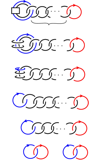
Figure 2. Kirby diagram of a Hopf link I.

2pt $L_{0}$ [br] at 3 71 $L_{1}$ [bl] at 11 52 $-1$ at 33 59 $0$ [bl] at 62 69 $0$ [tr] at 56 66 $L_{0}$ [br] at 84 71 $L_{1}$ [bl] at 92 52 $1$ [r] at 100 62 $1$ [bl] at 144 69 $1$ [tr] at 137 66 $L_{0}$ [br] at 18 22 $L_{1}$ [bl] at 64 22 $-1$ [tr] at 29 13 $L_{0}$ [br] at 88 22 $L_{1}$ [bl] at 123 18

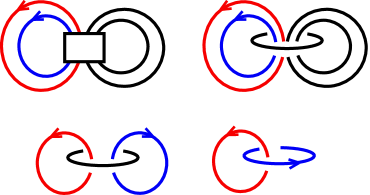
Figure 3. Kirby diagram of a Hopf link II.

2pt $L_{0}$ [br] at 22 76 $-2$ at 21 60 $-2$ [t] at 34 72 $-1$ at 53 60 $L_{1}$ [bl] at 76 76 $0/0/0$ [t] at 66 43 $L_{0}$ [br] at 104 76 $1$ [br] at 94 67 $1$ [tr] at 94 60 $1$ [br] at 123 64 $1$ [b] at 116 51 $L_{1}$ [bl] at 160 76 $1/1/1$ [t] at 149 43 $L_{0}$ [b] at 3 23 $1$ [r] at 0 16 $1$ [r] at 0 9 $1$ [bl] at 28 22 $-2$ [tl] at 43 13 $L_{1}$ [bl] at 56 22 $L_{0}$ [br] at 78 22 $L_{1}$ [bl] at 124 22 $-1$ [tl] at 112 14 $L_{0}$ [br] at 149 22 $L_{1}$ [b] at 179 21

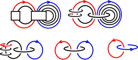
Figure 4. Kirby diagram of a Hopf link III.

2pt $L_{0}$ [br] at 12 148 $-2$ at 11 133 $-1$ [b] at 24 123 $-2$ [b] at 40 143 $-2$ [b] at 52 143 $-2$ [b] at 67 143 $-2$ [b] at 86 143 $-3$ [b] at 101 143 $-1$ at 117 133 $L_{1}$ [bl] at 141 148 $0/0/0$ [t] at 129 116 $n$ [t] at 65 114 $L_{0}$ [br] at 12 95 $1$ [r] at 0 85 $1$ [r] at 0 79 $1$ [b] at 24 69 $-2$ [b] at 39 89 $-2$ [b] at 52 89 $-2$ [b] at 67 89 $-2$ [b] at 86 89 $-2$ [b] at 101 89 $1$ [tr] at 104 77 $L_{1}$ [bl] at 141 95 $1/1/1$ [t] at 129 62 $n$ [t] at 64 60 $L_{0}$ [r] at 7 31 $1$ [r] at 7 25 $1$ [r] at 7 18 $1$ [b] at 25 37 $-2$ [b] at 37 33 $-2$ [b] at 52 33 $-2$ [b] at 67 33 $-2$ [b] at 86 33 $-2$ [b] at 101 33 $-2$ [tl] at 124 22 $L_{1}$ [bl] at 136 31 $n+2$ [t] at 75 0

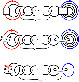
Figure 5. Kirby diagram of a Hopf link IV.