Bayesian Synthesis of Probabilistic Programs for Automatic Data ModelingDOI: 10.1145/3290350Journal: PACMPLVolume: 3POPL371CCS: Mathematics of computing Probability and statisticsCCS: Mathematics of computing Bayesian computationCCS: Mathematics of computing Markov-chain Monte Carlo methodsCCS: Mathematics of computing Time series analysisCCS: Mathematics of computing Multivariate statisticsCCS: Software and its engineering Domain specific languagesCCS: Theory of computation Probabilistic computationCCS: Theory of computation Bayesian analysisCCS: Theory of computation Data modelingCCS: Theory of computation Denotational semanticsCCS: Computing methodologies Machine learning

Abstract.

We present new techniques for automatically constructing probabilistic programs for data analysis, interpretation, and prediction. These techniques work with probabilistic domain-specific data modeling languages that capture key properties of a broad class of data generating processes, using Bayesian inference to synthesize probabilistic programs in these modeling languages given observed data. We provide a precise formulation of Bayesian synthesis for automatic data modeling that identifies sufficient conditions for the resulting synthesis procedure to be sound. We also derive a general class of synthesis algorithms for domain-specific languages specified by probabilistic context-free grammars and establish the soundness of our approach for these languages. We apply the techniques to automatically synthesize probabilistic programs for time series data and multivariate tabular data. We show how to analyze the structure of the synthesized programs to compute, for key qualitative properties of interest, the probability that the underlying data generating process exhibits each of these properties. Second, we translate probabilistic programs in the domain-specific language into probabilistic programs in Venture, a general-purpose probabilistic programming system. The translated Venture programs are then executed to obtain predictions of new time series data and new multivariate data records. Experimental results show that our techniques can accurately infer qualitative structure in multiple real-world data sets and outperform standard data analysis methods in forecasting and predicting new data.

1. Introduction

Data analysis is an important and longstanding activity in many areas of natural science, social science, and engineering (Tukey 1977; Gelman and Hill 2007). Within this field, probabilistic approaches that enable users to more accurately analyze, interpret, and predict underlying phenomena behind their data are rising in importance and prominence (Murphy 2012).

A primary goal of modern data modeling techniques is to obtain an artifact that explains the data. With current practice, this artifact takes the form of either a set of parameters for a fixed model (Nie 1975; Spiegelhalter et al. 1996; Plummer 2003; Cody and Smith 2005; Hyndman and Khandakar 2008; Rasmussen and Nickisch 2010; Seabold and Perktold 2010; Pedregosa et al. 2011; James et al. 2013) or a set of parameters for a fixed probabilistic program structure (Pfeffer 2001; Milch et al. 2005; Goodman et al. 2008; McCallum et al. 2009; Wood et al. 2014; Goodman and Stuhlmüller 2014; Carpenter et al. 2017; Pfeffer 2016; Salvatier et al. 2016; Tran et al. 2017; Ge et al. 2018). With this approach, users manually iterate over multiple increasingly refined models before obtaining satisfactory results. Drawbacks of this approach include the need for users to manually select the model or program structure, the need for significant modeling expertise, limited modeling capacity, and the potential for missing important aspects of the data if users do not explore a wide enough range of model or program structures.

In contrast to this current practice, we model the data with an ensemble of probabilistic programs sampled from a joint space of program structures and parameters. This approach eliminates the need for the user to select a specific model structure, extends the range of data that can be easily and productively analyzed, and (as our experimental results show) delivers artifacts that more accurately model the observed data. A challenge is that this approach requires substantially more sophisticated and effective probabilistic modeling and inference techniques.

We meet this challenge by combining techniques from machine learning, program synthesis, and programming language design. From machine learning we import the Bayesian modeling framework and the Bayesian inference algorithms required to express and sample from rich probabilistic structures. From program synthesis we import the concept of representing knowledge as programs and searching program spaces to derive solutions to technical problems. From programming language design we import the idea of using domain-specific languages to precisely capture families of computations. The entire framework rests on the foundation of a precise formal semantics which enables a clear formulation of the synthesis problem along with proofs that precisely characterize the soundness guarantees that our inference algorithms deliver.

1.1. Automated Data Modeling via Bayesian Synthesis of Probabilistic Programs in Domain-Specific Languages

We use Bayesian inference to synthesize ensembles of probabilistic programs sampled from domain-specific languages given observed data. Each language is designed to capture key properties of a broad class of data generating processes. Probabilistic programs in the domain-specific language (DSL) provide concise representations of probabilistic models that summarize the qualitative and quantitative structure in the underlying data generating process. The synthesized ensembles are then used for data analysis, interpretation, and prediction.

We precisely formalize the problem of Bayesian synthesis of probabilistic programs for automatic data modeling. To each expression in the domain-specific language we assign two denotational semantics: one that corresponds to the prior probability distribution over expressions in the DSL and another that corresponds to the probability distribution that each DSL expression assigns to new data. We provide sufficient conditions on these semantics needed for Bayesian synthesis to be well-defined. We outline a template for a broad class of synthesis algorithms and prove that algorithms that conform to this template and satisfy certain preconditions are sound, i.e., they converge asymptotically to the Bayesian posterior distribution on programs given the data.

Our approach provides automation that is lacking in both statistical programming environments and in probabilistic programming languages. Statistical programming environments such as SAS (Cody and Smith 2005), SPSS (Nie 1975) and BUGS (Spiegelhalter et al. 1996) require users to first choose a model family and then to write code that estimates model parameters. Probabilistic programming languages such as Stan (Carpenter et al. 2017), Figaro (Pfeffer 2016), and Edward (Tran et al. 2017) provide constructs that make it easier to estimate model parameters given data, but still require users to write probabilistic code that explicitly specifies the underlying model structure. Our approach, in contrast, automates model selection within the domain-specific languages. Instead of delivering a single model or probabilistic program, it delivers ensembles of synthesized probabilistic programs that, together, more accurately model the observed data.

1.2. Inferring Qualitative Structure by Processing Synthesized Programs

In this paper we work with probabilistic programs for model families in two domains: (i) analysis of univariate time series data via Gaussian processes (Rasmussen and Williams 2006); and (ii) analysis of multivariate tabular data using nonparametric mixture models (Mansinghka et al. 2016). The synthesized programs in the domain-specific language provide a compact model of the data that make qualitative properties apparent in the surface syntax of the program. We exploit this fact to develop simple program processing routines that automatically extract these properties and present them to users, along with a characterization of the uncertainty with which these properties are actually present in the observed data.

For our analysis of time series data, we focus on the presence or absence of basic temporal features such as linear trends, periodicity, and change points in the time series. For our analysis of multivariate tabular data, we focus on detecting the presence or absence of predictive relationships, which may be characterized by nonlinear or multi-modal patterns.

1.3. Predicting New Data by Translating Synthesized Programs to Venture

In addition to capturing qualitative properties, we obtain executable versions of the synthesized probabilistic programs specified in the DSL by translating them into probabilistic programs specified in Venture (Mansinghka et al. 2014). This translation step produces executable Venture programs that define a probability distribution over new, hypothetical data from a generative process learned from the observed data and that can deliver predictions for new data. Using Venture as the underlying prediction platform allows us to leverage the full expressiveness of Venture’s general-purpose probabilistic inference machinery to obtain accurate predictions, as opposed to writing custom prediction engines on a per-DSL basis.

For time series data analyzed with Gaussian processes, we use the Venture programs to forecast the time series into the future. For multivariate tabular data analyzed with mixture models, we use the programs to simulate new data with similar characteristics to the observed data.

1.4. Experimental Results

We deploy the method to synthesize probabilistic programs and perform data analysis tasks on several real-world datasets that contain rich probabilistic structure.

For time series applications, we process the synthesized Gaussian process programs to infer the probable existence or absence of temporal structures in multiple econometric time series with widely-varying patterns. The synthesized programs accurately report the existence of structures when they truly exist in the data and the absence of structures when they do not. We also demonstrate improved forecasting accuracy as compared to multiple widely-used statistical and baselines, indicating that they capture patterns in the underlying data generating processes.

For applications to multivariate tabular data, we show that synthesized programs report the existence of predictive relationships with nonlinear and multi-modal characteristics that are missed by standard pairwise correlation metrics. We also show that the predictive distribution over new data from the probabilistic programs faithfully represents the observed data as compared to simulations from generalized linear models and produce probability density estimates that are orders of magnitude more accurate than standard kernel density estimation techniques.

1.5. Contributions

This paper makes the following contributions:

• Bayesian synthesis of probabilistic programs. It introduces and precisely formalizes the problem of Bayesian synthesis of probabilistic programs for automatic data modeling in domain-specific data modeling languages. It also provides sufficient conditions for Bayesian synthesis to be well-defined. These conditions leverage the fact that expressions in the DSL correspond to data models and are given two denotational semantics: one that corresponds to the prior probability distribution over expressions in the DSL and another that corresponds to the probability distribution that each DSL expression assigns to new data. It also defines a template for a broad class of synthesis algorithms based on Markov chains and proves that algorithms which conform to this template and satisfy certain preconditions are sound, i.e., they converge to the Bayesian posterior distribution on programs given the data.

• Languages defined by probabilistic context-free grammars. It defines a class of domain-specific data modeling languages defined by probabilistic context-free grammars and identifies when these languages satisfy the sufficient conditions for sound Bayesian synthesis. We also provide an algorithm for Bayesian synthesis for this class of DSLs that conforms to the above template and prove that it satisfies the soundness preconditions.

• Example domain-specific languages for modeling time series and multivariate data. It introduces two domain-specific languages, each based on a state-of-the-art model discovery technique from the literature on Bayesian statistics and machine learning. These languages are suitable for modeling broad classes of real-world datasets.

• Applications to inferring qualitative structure and making quantitative predictions. It shows how to use the synthesized programs to (i) infer the probability that qualitative structure of interest is present in the data, by processing collections of programs produced by Bayesian synthesis, and (ii) make quantitative predictions for new data.

• Empirical results in multiple real-world domains. It presents empirical results for both inferring qualitative structure and predicting new data. The results show that the qualitative structures match the real-world data, for both domain specific languages, and can be more accurate than those identified by standard techniques from statistics. The results also show that the quantitative predictions are more accurate than multiple widely-used baselines.

2. Example

⬇

// ** PRIOR OVER DSL SOURCE CODE **

assume␣get_hyper␣~␣mem((node)␣~>␣{

␣␣-log_logistic(log_odds_uniform()␣#hypers:node)

});

assume␣choose_primitive␣=␣␣mem((node)␣~>␣{

␣␣base_kernel␣=␣uniform_discrete(0,␣5)␣#structure:node;

␣␣cond(

␣␣␣␣(base_kernel␣==␣0)(["WN",␣␣get_hyper(pair("WN",␣node))]),

␣␣␣␣(base_kernel␣==␣1)(["C",␣␣␣get_hyper(pair("C",␣node))]),

␣␣␣␣(base_kernel␣==␣2)(["LIN",␣get_hyper(pair("LIN",␣node))]),

␣␣␣␣(base_kernel␣==␣3)(["SE",␣␣get_hyper(pair("SE",␣node))]),

␣␣␣␣(base_kernel␣==␣4)(["PER",␣get_hyper(pair("PER_l",␣node)),

␣␣␣␣␣␣␣␣␣␣␣␣␣␣␣␣␣␣␣␣␣␣␣␣␣␣␣␣␣␣␣get_hyper(pair("PER_t",␣node))]))

});

assume␣choose_operator␣=␣mem((node)␣~>␣{

␣␣operator_symbol␣~␣categorical(

␣␣␣␣simplex(0.45,␣0.45,␣0.1),␣["+",␣"*",␣"CP"])

␣␣␣␣#structure:pair("operator",␣node);

␣␣if␣(operator_symbol␣==␣"CP")␣{

␣␣␣␣[operator_symbol,␣hyperprior(pair("CP",␣node)),␣.1]

␣␣}␣else␣{␣operator_symbol␣}

});

assume␣generate_random_dsl_code␣=␣mem((node)␣~>␣{

␣␣cov␣=␣if␣(flip(.3)␣#structure:pair("branch",␣node))␣{

␣␣␣␣operator␣~␣choose_operator(node);

␣␣␣␣[operator,

␣␣␣␣␣␣generate_random_dsl_code(2␣*␣node),

␣␣␣␣␣␣generate_random_dsl_code((2␣*␣node␣+␣1))]

␣␣}␣else␣{␣choose_primitive(node)␣};

␣␣["+",␣cov,␣["WN",␣0.01]]

});

assume␣dsl_source␣~␣generate_random_dsl_code(node:1);

⬇

// ** TRANSLATING DSL CODE INTO VENTURE **

assume␣ppl_source␣~␣generate_venturescript_code(dsl_source);

assume␣gp_executable␣=␣venture_eval(ppl_source);

⬇

// ** DATA OBSERVATION PROGRAM **

define␣xs␣=␣get_data_xs("./data.csv");

define␣ys␣=␣get_data_ys("./data.csv");

observe␣gp_executable(${xs})␣=␣ys;

⬇

// ** BAYESIAN SYNTHESIS PROGRAM **

resample(60);

for_each(arange(T),␣(_)␣->␣{

␣␣resimulate([|structure|],␣one,␣steps:100);

␣␣resimulate([|hypers|],␣one,␣steps:100)})

⬇

// ** PROCESSING SYNTHESIZED DSL CODE **

define␣count_kernels␣=␣(dsl,␣kernel)␣->␣{

␣␣if␣contains(["*",␣"+",␣"CP"],␣dsl[0])␣{

␣␣␣␣count_kernels(dsl[1],␣kernel)␣+␣count_kernels(dsl[2],␣kernel)

␣␣}␣else␣{␣if␣(kernel␣==␣dsl[0])␣{1}␣else␣{0}␣}

};

define␣count_operators␣=␣(dsl,␣operator)␣->␣{

␣␣if␣contains(["*",␣"+",␣"CP"],␣dsl[0])␣{

␣␣␣␣(if␣(operator␣==␣dsl[0])␣{1}␣else␣{0})

␣␣␣␣␣␣+␣count_operators(dsl[1],␣operator)

␣␣␣␣␣␣+␣count_operators(dsl[2],␣operator)

␣␣}␣else␣{␣0␣}

};

⬇

// ** SAMPLING FROM VENTURE EXECUTABLE FOR PREDICTION **

define␣xs_test␣=␣get_data_xs("./data.test.csv");

define␣ys_test␣=␣get_data_ys("./data.test.csv");

define␣ys_pred␣=␣sample_all(gp_executable(${xs_test}));

(a) Observed Dataset

⬇

>>␣plot(xs,␣ys,␣"Year",␣"Passenger Volume")

 

(b) Synthesized DSL and PPL Programs

⬇

>>␣sample_all(dsl_source)[0]

['+',

␣␣['*',

␣␣␣␣['+',␣['WN',49.5],␣['C',250.9]],

␣␣␣␣['+',␣['PER',␣13.2,␣8.6],

␣␣␣␣␣␣['+',

␣␣␣␣␣␣␣␣['LIN',␣1.2],

␣␣␣␣␣␣␣␣['LIN',␣4.9]]]],

␣␣['WN',␣0.1]]

>>␣sample_all(ppl_source)[0]

make_gp(gp_mean_const(0.),

␣␣((x1,x2)␣->␣{((x1,x2)␣->␣{((x1,x2)␣->

␣␣{((x1,x2)␣->

␣␣if␣(x1==x2)␣{49.5}␣else␣{0})(x1,x2)

␣␣␣␣+␣((x1,x2)␣->␣{250.9})(x1,x2)})(x1,x2)

␣␣␣␣*␣((x1,x2)␣->␣{((x1,x2)␣->␣{

␣␣␣␣-2/174.2400*sin(2*pi/8.6*

␣␣␣␣␣␣abs(x1-x2))**2})(x1,x2)

␣␣␣␣+␣((x1,x2)␣->␣{((x1,x2)␣->

␣␣␣␣{(x1-1.2)*(x2-1.2)})(x1,x2)

␣␣␣␣+␣((x1,x2)␣->

␣␣␣␣␣␣{(x1-4.9)*(x2-4.9)})(x1,x2)})

␣␣␣␣(x1,x2)})(x1,x2)})(x1,x2)

␣␣␣␣+␣((x1,x2)␣->␣if␣(x1==x2)␣{0.1}

␣␣␣␣else␣{0})(x1,x2)}))

 

(c) Processing Synthesized DSL Program

⬇

// estimate probability that data has

// change point or periodic structure

>>␣mean(mapv((prog)␣->␣{

␣␣␣␣count_kernels(prog,␣"PER")

␣␣␣␣+␣count_operators(prog,␣"CP")␣>␣0

␣␣},␣sample_all(dsl_source)))

0.97

 

(d) Predictions from PPL Program

⬇

>>␣plot(xs,␣ys,␣"Year",␣"Passenger Volume",

␣␣␣␣xs_test,␣ys_test,␣ys_pred)

Figure 2. Overview of Bayesian synthesis and execution of probabilistic programs in the Gaussian process DSL.

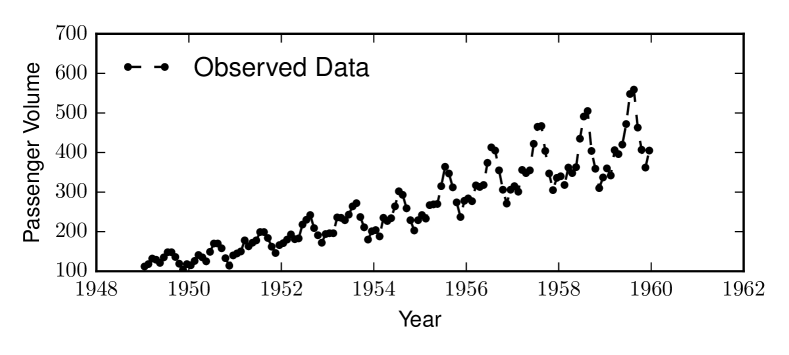
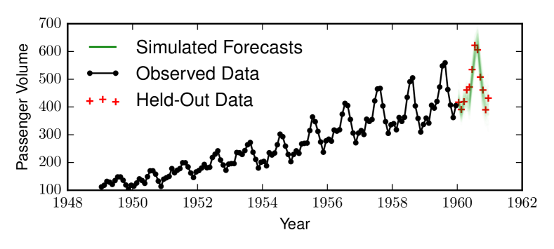
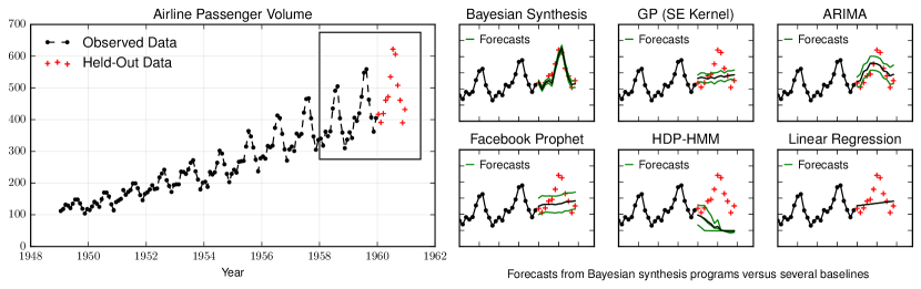
We next present an example that illustrates our synthesis technique and applications to data interpretation and prediction. Figure 2(d) presents a time series that plots world-wide airline passenger volume from 1948 to 1960 (Box and Jenkins 1976). The data contains the year and passenger volume data points. As is apparent from the time series plot, the data contain several temporal patterns. Passenger volume linearly increases over time, with periodic fluctuations correlated with the time of year — volume peaks in summer and falls in winter, with a small peak around winter vacation.

2.1. Gaussian Process Models

Gaussian processes (GPs) define a family of nonparametric regression models that are widely used to model a variety of data (Rasmussen and Williams 2006). It is possible to use GPs to discover complex temporal patterns in univariate time series (Duvenaud et al. 2013). We first briefly review the Gaussian process, which places a prior distribution over functions $f:\mathcal{X}\to\mathbb{R}$. In our airline passenger example, $x\in\mathcal{X}$ is a time point and $f(x)\in\mathbb{R}$ is passenger volume at time $x$. The GP prior can express both simple parametric forms, such as polynomial functions, as well as more complex relationships dictated by periodicity, smoothness, and time-varying functionals. Following notation of Rasmussen and Williams 2006, we formalize a GP $f\sim\mathsf{GP}(m,k)$ with mean function $m:\mathcal{X}\to\mathcal{Y}$ and covariance function $k:\mathcal{X}\times\mathcal{X}\to\mathbb{R}$ as follows: $f$ is a collection of random variables $\left\{f(x):x\in\mathcal{X}\right\}$. Give time points $\left\{x_{1},\dots,x_{n}\right\}$ the vector of random variables $[f(x_{1}),\dots,f(x_{n})]$ is jointly Gaussian with mean vector $[m(x_{1}),\dots,m(x_{n})]$ and covariance matrix $[k(x_{i},x_{j})]_{1\leq{i,j}\leq{n}}$.

The prior mean is typically set to zero (as it can be absorbed by the covariance). The functional form of the covariance $k$ defines essential features of the unknown function $f$, allowing the GP to (i) fit structural patterns in observed data, and (ii) make time series forecasts. GP covariance functions (also called kernels) can be created by composing a set of simple base kernels through sum, product, and change point operators (Rasmussen and Williams 2006, Section 4.2). We therefore define the following domain-specific language for expressing the covariance function of a specific GP:

$$K\in\mathsf{Kernel} \Coloneqq\texttt{(}\texttt{C}\;v\texttt{)}\mid\texttt{(}\texttt{WN}\;v\texttt{)}\mid\texttt{(}\texttt{SE}\;v\texttt{)}\mid\texttt{(}\texttt{LIN}\;v\texttt{)}\mid\texttt{(}\texttt{PER}\;v_{1}\;v_{2}\texttt{)} \mathrm{[BaseKernels]}$$

$$\mid\texttt{(}\texttt{+}\;K_{1}\;K_{2}\texttt{)}\mid\texttt{(}\texttt{$\times$}\;K_{1}\;K_{1}\texttt{)}\mid\texttt{(}\texttt{CP}\;v\;K_{1}\;K_{2}\texttt{)} \mathrm{[CompositeKernels]}$$

The base kernels are constant (C), white noise (WN), squared exponential (SE), linear (LIN), and periodic (PER). Each base kernel has one or more numeric parameters $v$. For example, LIN has an x-intercept and PER has a length scale and period. The composition operators are sum ($+$), product ($\times$), and change point (CP, which smoothly transitions between two kernels at some x-location). Given a covariance function specified in this language, the predictive distribution over airline passenger volumes $[f(x_{1}),\dots,f(x_{n})]$ at time points $(x_{1},\dots,x_{n})$ is a standard multivariate normal.

2.2. Synthesized Gaussian Process Model Programs

The first code box in Figure 2 (lines 148-171) presents Venture code that defines a prior distribution over programs in our domain-specific Gaussian process language. This code implements a probabilistic context-free grammar that samples a specific program from the DSL. In the code box, we have two representations of the program: (i) a program in the domain-specific language (dsl_source, line 169); and (ii) the translation of this program into executable code in the Venture probabilistic programming language (ppl_source, line 171). When evaluated using venture_eval, the translated Venture code generates a stochastic procedure that implements the Gaussian process model (gp_executable, line 172). Given the observed time points (xs, line 173 of the second code box in Figure 2), the stochastic procedure gp_executable defines the probability of observing the corresponding passenger volume data (ys, line 174) according to the GP. This probability imposes a posterior distribution on the random choices made by generate_random_dsl_code (line 163) which sampled the dsl_source. The next step is to perform Bayesian inference over these random choices to obtain a collection of programs (approximately) sampled from this posterior distribution. Programs sampled from the posterior tend to deliver a good fit between the observed data and the Gaussian process. In our example we configure Venture to sample 60 programs from the (approximately inferred) posterior (line 176). The third code box in Figure 2 actually performs the inference, specifically by using a Venture custom inference strategy that alternates between performing a Metropolis-Hastings step over the program structure (base kernels and operators) and a Metropolis-Hastings step over the program parameters (lines 177-179).

2.3. Inferring Qualitative Structure by Processing Synthesized Programs

Figure 2(d) presents one of the programs sampled from the posterior. The syntactic structure of this synthesized program reflects temporal structure present in the airline passenger volume data. Specifically, this program models the data as the sum of linear and periodic components (base kernels) along with white noise. Of course, this is only one of many programs (in our example, 60 programs) sampled from the posterior. To analyze the structure that these programs expose in the data, we check for the existence of different base kernels and operators in each program (fourth code box in Figure 2 and Figure 2(d)). By averging across the ensemble of synthesized program we estimate the probable presence of each structure in the data. In our example, all of the programs have white noise, 95% exhibit a linear trend, 95% exhibit periodicity, and only 22% contain a change point. These results indicate the likely presence of both linear and periodic structure.

2.4. Predicting New Data via Probabilistic Inference

In addition to supporting structure discovery by processing the synthesized domain-specific program (dsl_source), it is also possible to sample new data directly from the Venture executable (gp_executable) obtained from the translated program (ppl_source). In our example, this capability makes it possible to forecast future passenger volumes. The final code box in Figure 2 presents one such forecast, which we obtain by sampling data from the collection of 60 synthesized stochastic procedures (the green line in Figure 2(d) overlays all the sampled predictions). The forecasts closely match the actual held-out data, which indicates that the synthesized programs effectively capture important aspects of the underlying temporal structure in the actual data.

3. Bayesian Synthesis in Domain-Specific Data Modeling Languages

Figure 3. Components of Bayesian synthesis of probabilistic programs for automatic data modeling.

We next present a general framework for Bayesian synthesis in probabilistic domain-specific languages. We formalize the probabilistic DSL $\mathcal{L}$ as a countable set of strings, where an expression $E\in\mathcal{L}$ represents the structure and parameters of a family of statistical models specified by the DSL (such as the space of all Gaussian process models from Section 2). We associate $\mathcal{L}$ with a pair of denotational semantics $\mathsf{Prior}$ and $\mathsf{Lik}$ that describe the meaning of expressions $E$ in the language:

• The “prior” semantic function $\mathsf{Prior}:\mathcal{L}\to(0,1]$, where $\mathsf{Prior}\left\llbracket E\right\rrbracket$ is a positive real number describing the probability that a given random process generated $E$.

• The “likelihood” semantic function $\mathsf{Lik}:\mathcal{L}\to(\mathcal{X}\to\mathbb{R}_{\geq 0})$, where $\mathsf{Lik}\left\llbracket E\right\rrbracket$ is a probability function over a data space $\mathcal{X}$, where each item $X\in\mathcal{X}$ has a relative probability $\mathsf{Lik}\left\llbracket E\right\rrbracket(X)$.

These two semantic functions are required to satisfy three technical conditions.

Condition 3.1 (Normalized Prior).

$\mathsf{Prior}$ defines a valid probability distribution over $\mathcal{L}$:

(1) $$\sum_{E\in\mathcal{L}}\mathsf{Prior}\left\llbracket E\right\rrbracket=1.$$

If $\mathcal{L}$ is finite then this condition can be verified directly by summing the values. Otherwise if $\mathcal{L}$ is countably infinite then a more careful analysis is required (see Section 4.2).

Condition 3.2 (Normalized Likelihood).

For each $E\in\mathcal{L}$, $\mathsf{Lik}\left\llbracket E\right\rrbracket$ is a probability distribution (for countable data) or density (for continuous data) over $\mathcal{X}$:

(2) $$\forall E\in\mathcal{L}.\begin{cases}\sum_{X\in\mathcal{X}}\mathsf{Lik}\left\llbracket E\right\rrbracket(X)=1&\textrm{(if $\mathcal{X}$ is a countable space)}\\ \int_{X\in\mathcal{X}}\mathsf{Lik}\left\llbracket E\right\rrbracket(X)\mu(dX)=1&\textrm{(if $\mathcal{X}$ is a general space with base measure $\mu$)}.\end{cases}$$

Condition 3.3 (Bounded Likelihood).

$\mathsf{Lik}$ is bounded, and is non-zero for some expression $E$:

(3) $$\forall X\in\mathcal{X}.\;0<c^{\max}_{X}\Coloneqq\sup\left\{\mathsf{Lik}\left\llbracket E\right\rrbracket(X)\mid E\in\mathcal{L}\right\}<\infty.$$

For each $X\in\mathcal{X}$, define $c_{X}\Coloneqq\sum_{E\in\mathcal{L}}\mathsf{Lik}\left\llbracket E\right\rrbracket(X)\cdot\mathsf{Prior}\left\llbracket E\right\rrbracket$ to be the marginal probability of $X$ (which is finite by Conditions 3.1 and 3.3). When the semantic functions satisfy the above conditions, they induce a new semantic function $\mathsf{Post}:\mathcal{L}\to\mathcal{X}\to\mathbb{R}_{\geq{0}}$, called the posterior distribution:

(4) $$\mathsf{Post}\left\llbracket E\right\rrbracket(X) \Coloneqq(\mathsf{Lik}\left\llbracket E\right\rrbracket(X)\;\mathsf{Prior}\left\llbracket E\right\rrbracket)/c_{X}.$$

Lemma 3.4.

Let $\mathcal{L}$ be a language whose denotational semantics $\mathsf{Prior}$ and $\mathsf{Lik}$ satisfy Conditions 3.1, 3.2, and 3.3. For each $X\in\mathcal{X}$, the function $\lambda E.\mathsf{Post}\left\llbracket E\right\rrbracket(X)$ is a probability distribution over $\mathcal{L}$.

Proof.

Fix $X$. Then $\sum_{E\in\mathcal{L}}\mathsf{Post}\left\llbracket E\right\rrbracket(X)=\sum_{E\in\mathcal{L}}(\mathsf{Lik}\left\llbracket E\right\rrbracket(X)\;\mathsf{Prior}\left\llbracket E\right\rrbracket)/c_{X}=c_{X}/c_{X}=1.$ ∎

The objective of Bayesian synthesis can now be stated.

Objective 3.5 (Bayesian Synthesis).

Let $\mathcal{L}$ be a language whose denotational semantics $\mathsf{Prior}$ and $\mathsf{Lik}$ satisfy Conditions 3.1, 3.2, and 3.3. Given a dataset $X\in\mathcal{X}$, generate expressions $E$ with probability $\mathsf{Post}\left\llbracket E\right\rrbracket(X)$.

Figure 3 shows the main components of our approach. Assuming we can achieve the objective of Bayesian synthesis, we now outline how to use synthesized probabilistic programs in the DSL for (i) inferring qualitative statistical structure, by using simple program analyses on the program text; and (ii) predicting new data by translating them into executable Venture probabilistic programs.

3.1. Inferring Probabilities of Qualitative Properties in Synthesized DSL Programs

After synthesizing an ensemble of $n$ DSL expressions $\left\{E_{1},\dots,E_{n}\right\}$ according to the posterior probability distribution given $X$, we can obtain insight into the learned models by processing the synthesized DSL expressions. In this paper, a typical query has the signature $\mathsf{HasProperty}:\mathcal{L}\to\left\{0,1\right\}$ that checks whether a particular property holds in a given DSL program. In other words, $\mathsf{HasProperty}\left\llbracket E\right\rrbracket$ is 1 if the $E$ reflects the property, and 0 otherwise. We can use the synthesized programs to form an unbiased estimate of the posterior probability of a property:

(5) $$\Pr\left\{\mathsf{HasProperty}\left\llbracket E\right\rrbracket\mid X\right\}\approx\frac{1}{n}\sum_{i=1}^{n}\mathsf{HasProperty}\left\llbracket E_{i}\right\rrbracket.$$

3.2. Forming Predictions by Translating DSL Programs into Venture Programs

In our formalism, each DSL expression $E\in\mathcal{L}$ is a probabilistic program that represents the structure and parameters of a family of statistical models specified by the domain-specific language. In this paper, we translate probabilistic programs $E$ in the DSL into new probabilistic programs $\mathsf{Venture}\left\llbracket E\right\rrbracket$ specified in Venture (Mansinghka et al. 2014). A main advantage of translating DSL programs into Venture programs is that we can reuse general-purpose inference machinery in Venture (Mansinghka et al. 2018) to obtain accurate predictions, as opposed to writing custom interpreters for data prediction on a per-DSL basis. Sections 5 and 6 show two concrete examples of how DSL programs can be translated into Venture programs and how to use inference programming in Venture to obtain predictions on new data.

3.3. Markov Chain Monte Carlo Algorithms for Bayesian Synthesis

We next describe Markov chain Monte Carlo (MCMC) techniques to randomly sample expressions $E\in\mathcal{L}$ with probability that approximates $\mathsf{Post}\left\llbracket E\right\rrbracket(X)$ to achieve Objective 3.5. In particular, we employ a general class of MCMC sampling algorithms (Algorithm 1) that first obtains an expression $E_{0}\in\mathcal{L}$ such that $\mathsf{Lik}\left\llbracket E\right\rrbracket(X)>0$ and then iteratively generates a sequence of expressions $E_{1},\ldots,E_{n}\in\mathcal{L}$. The algorithm iteratively generates $E_{i}$ from $E_{i-1}$ using a DSL-specific transition operator $\mathcal{T}$, which takes as input expression $E\in\mathcal{L}$ and a data set $X$, and stochastically samples an expression $E^{\prime}$ with probability denoted $\mathcal{T}(X,E\to E^{\prime})$, where $\sum_{E^{\prime}\in\mathcal{L}}\mathcal{T}(X,E\to E^{\prime})=1$ for all $E\in\mathcal{L}$. The algorithm returns the final expression $E_{n}$. Implementing Bayesian synthesis for a data-modeling DSL $\mathcal{L}$ requires implementing three procedures:

1. generate-expression-from-prior, which generates expression $E$ with probability $\mathsf{Prior}\left\llbracket E\right\rrbracket$.

2. $\textsc{evaluate-likelihood}(X,E)$, which evaluates $\mathsf{Lik}\left\llbracket E\right\rrbracket(X)$.

3. $\textsc{generate-new-expression}(X,E)$, which generates expression $E^{\prime}$ from expression $E$ with probability $\mathcal{T}(X,E\to E^{\prime})$.

Algorithm 1 Template of Markov chain Monte Carlo algorithm for Bayesian synthesis.

1: procedure bayesian-synthesis($X$, $\mathcal{T}$, $n$)

2:   do

3:    $E_{0}\sim\textsc{generate-expression-from-prior}()$

4:   while $\mathsf{Lik}\left\llbracket E_{0}\right\rrbracket(X)=0$

5:   for $i=1\ldots n$ do

6:    $E_{i}\sim\textsc{generate-new-expression}(X,E_{i-1}))$   

7:   return $E_{n}$

Using MCMC for synthesis allows us to rigorously characterize soundness conditions. We now describe three conditions on the operator $\mathcal{T}$ that are sufficient to show that Algorithm 1 generates expressions from arbitrarily close approximation to the Bayesian posterior distribution on expressions $\mathsf{Post}\left\llbracket E\right\rrbracket(X)$. In Section 4.3 we show how to construct such an operator for a class of DSLs generated by probabilistic context-free grammars and prove that this operator satisfies the conditions.

Condition 3.6 (Posterior invariance).

If an expression $E$ is sampled from the posterior distribution and a new expression $E^{\prime}\in\mathcal{L}$ is sampled with probability $\mathcal{T}(X,E\to E^{\prime})$, then $E^{\prime}$ is also a sample from the posterior distribution:

$$\sum_{E\in\mathcal{L}}\mathsf{Post}\left\llbracket E\right\rrbracket(X)\cdot\mathcal{T}(X,E\to E^{\prime})=\mathsf{Post}\left\llbracket E^{\prime}\right\rrbracket(X).$$

Condition 3.7 (Posterior irreducibility).

Every expression $E^{\prime}$ with non-zero likelihood is reachable from every expression $E\in\mathcal{L}$ in a finite number of steps. That is, for all pairs of expressions $E\in\mathcal{L}$ and $E^{\prime}\in\{\mathcal{L}:\mathsf{Lik}\left\llbracket E^{\prime}\right\rrbracket(X)>0\}$ there exists an integer $n\geq 1$ and a sequence of expressions $E_{1},E_{2},\ldots,E_{n}$ where $E_{1}=E$ and $E_{n}=E^{\prime}$ such that $\mathcal{T}(X,E_{i-1}\to E_{i})>0$ for all $i\in\{2,\ldots n\}$.

Condition 3.8 (Aperiodicity).

There exists some expression $E\in\mathcal{L}$ such that the transition operator has a non-zero probability of returning to the same expression, i.e. $\mathcal{T}(X,E\to E)>0$.

We now show that Algorithm 1 gives asymptotically correct results provided these three conditions hold. First, we show that it is possible to obtain an expression $E_{0}\in\mathcal{L}$ where $\mathsf{Lik}\left\llbracket E_{0}\right\rrbracket(X)>0$ using a finite number of invocations of generate-expression-from-prior.

Lemma 3.9.

The do-while loop of Algorithm 1 will terminate with probability 1, and the expected number of iterations in the do-while loop is at most $c_{X}^{\max}/c_{X}$.

Proof.

The number of iterations of the loop is geometrically distributed with mean $p$, given by:

$$p =\sum_{E\in\mathcal{L}}\mathsf{Prior}\left\llbracket E\right\rrbracket\cdot\mathbb{I}[\mathsf{Lik}\left\llbracket E\right\rrbracket(X)>0]=\frac{1}{c_{X}^{\max}}\sum_{E\in\mathcal{L}}\mathsf{Prior}\left\llbracket E\right\rrbracket\cdot c^{\max}_{X}\cdot\mathbb{I}[\mathsf{Lik}\left\llbracket E\right\rrbracket(X)>0]$$

$$\geq\frac{1}{c_{X}^{\max}}\sum_{E\in\mathcal{L}}\mathsf{Prior}\left\llbracket E\right\rrbracket\cdot\mathsf{Lik}\left\llbracket E\right\rrbracket(X)=\frac{c_{X}}{c_{X}^{\max}}.$$

Therefore, the expected number of iterations of the do-while loop is at most $1/p=c_{X}^{\max}/c_{X}<\infty$. ∎

We denote the probability that Algorithm 1 returns expression $E$, given that it started with expression $E_{0}$ by $\mathsf{ApproxPost}{{}_{E_{0}}^{1}}\left\llbracket E\right\rrbracket(X)$, and define the $n$-step probability inductively:

$$\mathsf{ApproxPost}{{}_{E_{0}}^{1}}\left\llbracket E\right\rrbracket(X) \Coloneqq\mathcal{T}(X,E_{0}\to E)$$

$$\mathsf{ApproxPost}{{}_{E_{0}}^{n}}\left\llbracket E\right\rrbracket(X) \Coloneqq\sum_{E^{\prime}\in\mathcal{L}}\mathcal{T}(X,E^{\prime}\to E)\cdot\mathsf{ApproxPost}{{}_{E_{0}}^{n-1}}\left\llbracket E^{\prime}\right\rrbracket(X) (n>1).$$

We can now state a key convergence theorem, due to Tierney 1994.

Theorem 3.10 (Convergence of MCMC (Tierney 1994)).

If Condition 3.6 and Condition 3.7 and Condition 3.8 hold for some language $\mathcal{L}$, transition operator $\mathcal{T}$, and data $X\in\mathcal{X}$, then

$$\forall E_{0},E\in\mathcal{L}.\;\mathsf{Lik}\left\llbracket E_{0}\right\rrbracket(X)>0\implies\lim_{n\to\infty}\mathsf{ApproxPost}{{}_{E_{0}}^{n}}\left\llbracket E\right\rrbracket(X)\to\mathsf{Post}\left\llbracket E\right\rrbracket(X).$$

4. Bayesian Synthesis for Domain-Specific Languages Defined By Probabilistic Context-Free Grammars

Having described the general framework for Bayesian synthesis in general domain-specific languages, we now focus on the class of domain-specific languages which are generated by a probabilistic context-free grammar (PCFG) over symbolic expressions (s-expressions). We begin by describing the formal model of the grammar and the languages it can produce. We then outline a default denotational semantics $\mathsf{Prior}$, derive a general MCMC algorithm for all languages in this class, and prove that the synthesis technique converges to the posterior distribution over expressions.

4.1. Tagged Probabilistic Context-Free Grammars with Random Symbols

Probabilistic context-free grammars are commonly used models for constructing languages (Jelinek et al. 1992). We describe a special type of PCFG, called a tagged PCFG with random symbols, by extending the standard definition in two ways: (i) we require the grammar to produce s-expressions containing a unique phrase tag for each production rule, which guarantees that the grammar is unambiguous; and (ii) we allow each non-terminal to specify a probability distribution over symbols in the alphabet. The model is formally described below.

Definition 4.1 (Tagged probabilistic context-free grammar with random symbols).

A tagged probabilistic context-free grammar with random symbols is a tuple $G=(\Sigma,N,R,T,P,Q,S)$ where

• $\Sigma$ is a finite set of terminal symbols.

• $N\Coloneqq\left\{N_{1},\dots,N_{m}\right\}$ is a finite set of non-terminal symbols.

• $R\Coloneqq\left\{R_{ik}\mid i=1,\dots,m;k=1,\dots,r_{i}\right\}$ is a set of production rules, where $R_{ik}$ is the $k\textsuperscript{th}$ production rule of non-terminal $N_{i}$. Each production rule $R_{ik}$ is a tuple of the form

  (6) $$R_{ik} \Coloneqq(N_{i},T_{ik},\tilde{N}_{1}\cdots\tilde{N}_{h_{ik}}),$$

  where $h_{ik}\geq 0$ is the number of non-terminals on the right-hand side of $R_{ik}$ and each $\tilde{N}_{j}\in N$ $(j=1,2,\dots,h_{ik})$ is a non-terminal symbol. If $h_{ik}=0$ then $\tilde{N}_{1}\cdots\tilde{N}_{h_{ik}}=\epsilon$ is the empty string and we call $R_{ik}$ a non-recursive production rule. Otherwise it is a recursive rule.

• $T\Coloneqq\left\{T_{ik}\mid i=1,\dots,m;k=1,\dots,r_{i}\right\}$ is a set of phrase tag symbols, disjoint from $N$, where $T_{ik}$ is a unique symbol identifying the production rule $R_{ik}$.

• $P:T\to(0,1]$ is a map from phrase tag symbols to their probabilities, where $P(T_{ik})$ is the probability that non-terminal $N_{i}$ selects its $k\textsuperscript{th}$ production rule $R_{ik}$. For each non-terminal $N_{i}$, the probabilities over its production rules sum to unity $\sum_{k=1}^{r_{i}}P(T_{ik})=1$.

• $Q:T\times\Sigma\to[0,1]$ is a map from phrase tags and terminal symbols to probabilities, where $Q(T_{ik},s)$ is the probability that production rule $R_{ik}$ of non-terminal $N_{i}$ draws the terminal symbol $s\in\Sigma$. For each tag $T_{ik}$, the probabilities over symbols sum to unity $\sum_{s\in\Sigma}Q(T_{ik},s)=1$.

• $S\in N$ is a designated start symbol.

We additionally assume that grammar $G$ is proper: production rules must be cycle-free, and there are no useless symbols in $\Sigma\cup N\cup T$ (Nijholt 1980).

The production rules from Eq (6) define the rewriting rules that describe how to syntactically replace a non-terminal $N_{i}$ with a tagged s-expression. We now describe how an evaluator uses these production rules to generate tagged s-expressions according to the probabilities $P$ and $Q$. The big-step sampling semantics for this evaluator are shown below, where the notation $N_{i}\Downarrow^{p}_{G}E$ means that starting from non-terminal $N_{i}$, the evaluator yielded expression $E$ with $p$ being the total probability of all the phrase tags and terminal symbols in the generated s-expression.

[Sampling: Non-Recursive Production Rule] [Sampling: Recursive Production Rule]

$$N_{i}\Downarrow^{P(T_{ik})Q(T_{ik},s)\phantom{\prod_{z=1}^{h_{ik}}{p_{z}}}}_{G}\hskip-25.00003pt(T_{ik}\;s)(N_{i},T_{ik},\epsilon)\in R,\,s\in\Sigma,\,Q(T_{ik},s)>0 N_{i}\Downarrow^{P(T_{ik})\prod_{z=1}^{h_{ik}}{p_{z}}}_{G}(T_{ik}\;E_{1}\;\dots\;E_{h_{ik}})(N_{i},T_{ik},\tilde{N}_{1}\cdots\tilde{N}_{h_{ik}})\in R,\;\tilde{N}_{1}\Downarrow^{p_{1}}_{G}E_{1},\;\dots,\;\tilde{N}_{h_{ik}}\Downarrow^{p_{h_{ik}}}_{G}E_{j}$$

In words, when the evaluator encounters a non-terminal symbol $N_{i}$, it chooses a production rule $R_{ik}$ with probability $P(T_{ik})$. If the selected production rule is non-recursive, the evaluator randomly samples a symbol $s\in\Sigma$ with probability $Q(T_{ik},s)$, and returns an s-expression starting with $T_{ik}$ followed by the random symbol. Otherwise, if the selected production rule is recursive, the evaluator recursively evaluates all the constituent non-terminals and returns an s-expression starting with $T_{ik}$ followed by all the evaluated sub-expressions. Note that each evaluation step yields an s-expression where the first element is a phrase tag $T_{ik}$ that unambiguously identifies the production rule $R_{ik}$ that was selected to produce the expression. Hence, every expression maps uniquely to its corresponding parse tree simply by reading the phrase tags (Turbak et al. 2008). As a result, the probability of any expression under its sampling semantics is unambiguous which is essential for the soundness properties established in Section 4.3.

Finally, we let $\mathcal{L}(G,N_{i})$ denote the set of all strings that can be yielded starting from non-terminal $N_{i}$ $(i=1,\dots,m)$, according to the sampling semantics $\Downarrow_{G}$. The language $\mathcal{L}(G)$ generated by $G$ is the set of all strings derivable from the start symbol $S$, so that $\mathcal{L}(G)\Coloneqq\mathcal{L}(G,S)$. Conceptually, for a probabilistic domain-specific language $\mathcal{L}$ specified by tagged PCFGs, terminal symbols $s\in\Sigma$ are used to represent the program parameters and tag symbols $t\in T$ represent the program structure.

4.2. A Default Prior Semantics with the Normalization Property

Having described the big-step sampling semantics for expressions $E\in\mathcal{L}$ generated by a tagged probabilistic context-free grammar $G$, we next describe the “prior” denotational semantics of an expression, given by the semantic function $\mathsf{Prior}:\mathcal{L}(G)\to(0,1]$. To aid with the construction, we first introduce some additional notation. Define the semantic function $\mathsf{Expand}:\mathcal{L}(G)\to N\to[0,1]$ which takes an expression and a non-terminal symbol, and returns the probability that the non-terminal evaluates to the given expression:

$$\mathsf{Expand}\left\llbracket(T_{ik}\;s)\right\rrbracket(N_{i}) \Coloneqq P(T_{ik})\cdot Q(T_{ik},s)$$

$$\mathsf{Expand}\left\llbracket(T_{ik}\;E_{1}\;\cdots\;E_{h_{ik}})\right\rrbracket(N_{i}) \Coloneqq P(T_{ik})\cdot\textstyle\prod_{z=1}^{h_{ik}}\mathsf{Expand}\left\llbracket E_{z}\right\rrbracket(\tilde{N}_{z})$$

$$\;\mbox{where }R_{ik}=(T_{ik},N_{i},\tilde{N}_{1},\dots,\tilde{N}_{h_{ik}}),$$

for $i=1,\dots,n$ and $k=1,\dots,r_{i}$.

Lemma 4.2.

For each non-terminal $N_{i}$ and for all expressions $E\in\mathcal{L}(G,N_{i})$, we have

$$\mathsf{Expand}\left\llbracket E\right\rrbracket(N_{i})=p\mbox{ if and only if }N_{i}\Downarrow^{p}_{G}E.$$

Proof.

By structural induction on the s-expression $E$. ∎

Recalling that $S$ is the start symbol of $G$, we define the prior semantics

(7) $$\mathsf{Prior}\left\llbracket E\right\rrbracket\Coloneqq\mathsf{Expand}\left\llbracket E\right\rrbracket(S).$$

Having established the correspondence between the sampling semantics and denotational semantics, we next provide necessary and sufficient conditions on $G$ that are needed for $\mathsf{Prior}$ to be properly normalized as required by Condition 3.1. We begin with the following definition:

Definition 4.3 (Consistency (Booth and Thompson 1973)).

A probabilistic context-free grammar $G$ is consistent if the probabilities assigned to all words derivable from $G$ sum to 1.

The following result of Booth and Thompson 1973 plays a key role in our construction.

Theorem 4.4 (Sufficient Condition for Consistency (Booth and Thompson 1973)).

A proper probabilistic context-free grammar $G$ is consistent if the largest eigenvalue (in modulus) of the expectation matrix of $G$ is less than 1.

The expectation matrix of $G$ can be computed explicitly using the transition rule probabilities $P$ for non-terminal symbols (Gecse and Kovács 2010, Equation 2). If $G$ is non-recursive then it is necessarily consistent since $\mathcal{L}(G)$ consists of a finite number of finite length words. Otherwise, if $G$ is recursive, consistency is equivalently described by having the expected number of steps in the stochastic rewriting-process $\Downarrow_{G}$ be finite Gecse and Kovács 2010. To ensure that the $\mathsf{Prior}$ semantic function of $G$ is correctly normalized, we construct the expectation matrix and confirm that the modulus of the largest eigenvalue is less than 1. (Note that the probabilities $Q$ of random symbols in the tagged PCFG are immaterial in the analysis, since they appear only in non-recursive production rules and do not influence the production rule probabilities $P$.) We henceforth require every tagged probabilistic context-free grammar to satisfy the stated conditions for consistency.

4.3. Bayesian Synthesis Using Markov Chain Monte Carlo

We now derive a Bayesian synthesis algorithm specialized to domain-specific languages which are generated by a tagged context-free grammar, and prove that the algorithm satisfies the conditions for convergence in Theorem 3.10. Recall that implementing Algorithm 1 requires an implementation of three procedures:

1. generate-expression-from-prior, which generates expression $E$ with probability $\mathsf{Prior}\left\llbracket E\right\rrbracket$ (subject to Condition 3.1). Letting $E\sim\mathsf{Expand}\left\llbracket\cdot\right\rrbracket(N_{i})$ mean that $E$ is sampled randomly with probability $\mathsf{Expand}\left\llbracket E\right\rrbracket(N_{i})$ $(N_{i}\in N)$, we implement this procedure by sampling $E\sim\mathsf{Expand}\left\llbracket\cdot\right\rrbracket(S)$ as described in Section 4.2.

2. $\textsc{evaluate-likelihood}(X,E)$, which evaluates $\mathsf{Lik}\left\llbracket E\right\rrbracket(X)$ (subject to Conditions 3.2 and 3.3). This procedure is DSL specific; two concrete examples are given in Sections 5 and 6.

3. $\textsc{generate-new-expression}(X,E)$, which generates a new expression $E^{\prime}$ from the starting expression $E$ with probability $\mathcal{T}(X,E\to E^{\prime})$ (subject to Conditions 3.7, 3.6, and 3.8), which we describe below.

We construct a class of transition operators $\mathcal{T}(X,E\to E^{\prime})$ that (i) stochastically replaces a random sub-expression in $E$; then (ii) stochastically accepts or rejects the mutation depending on how much it increases (or decreases) the value of $\mathsf{Lik}\left\llbracket E\right\rrbracket(X)$. Our construction applies to any data-modeling DSL generated by a tagged PCFG and is shown in Algorithm 2. In this section we establish that the transition operator in Algorithm 2 satisfies Conditions 3.7, 3.6, and 3.8 for Bayesian synthesis with Markov chain Monte Carlo given in Section 3.3.

Algorithm 2 Transition operator $\mathcal{T}$ for a context-free data-modeling language.

1: procedure generate-new-expression($E,X$) $\triangleright$ Input expression $E$ and data set $X$

2:   $a\sim\mbox{SelectRandomElementUniformly}(A_{E})$ $\triangleright$ Randomly select a node in parse tree

3:   $(N_{i},E_{\mathsf{hole}})\leftarrow\mathsf{Sever}_{a}\left\llbracket E\right\rrbracket$ $\triangleright$ Sever the parse tree and return the non-terminal symbol at the sever point

4:   $E_{\mathsf{sub}}\sim\mathsf{Expand}\left\llbracket\cdot\right\rrbracket(N_{i})$ $\triangleright$ Generate random $E_{\mathsf{sub}}$ with probability $\mathsf{Expand}\left\llbracket E_{\mathsf{sub}}\right\rrbracket(N_{i})$

5:   $E^{\prime}\leftarrow E_{\mathsf{hole}}[E_{\mathsf{sub}}]$ $\triangleright$ Fill hole in $E_{\mathsf{hole}}$ with expression $E_{\mathsf{sub}}$

6:   $L\leftarrow\mathsf{Lik}\left\llbracket E\right\rrbracket(X)$ $\triangleright$ Evaluate likelihood for expression $E$ and data set $X$

7:   $L^{\prime}\leftarrow\mathsf{Lik}\left\llbracket E^{\prime}\right\rrbracket(X)$ $\triangleright$ Evaluate likelihood for expression $E^{\prime}$ and data set $X$

8:   $p_{\mathsf{accept}}\leftarrow\min\left\{1,(|A_{E}|/|A_{E^{\prime}}|)\cdot(L^{\prime}/L)\right\}$ $\triangleright$ Compute the probability of accepting the mutation

9:   $r\sim\mbox{UniformRandomNumber}([0,1])$ $\triangleright$ Draw a random number from the unit interval

10:   if $r<p_{\mathsf{accept}}$ then $\triangleright$ If-branch has probability $p_{\mathsf{accept}}$

11:    return $E^{\prime}$ $\triangleright$ Accept and return the mutated expression

12:   else$\triangleright$ Else-branch has probability $1-p_{\mathsf{accept}}$

13:    return $E$ $\triangleright$ Reject the mutated expression, and return the input expression   

Let $G$ be a grammar from Definition 4.1 with language $\mathcal{L}\Coloneqq\mathcal{L}(G)$. We first describe a scheme for uniquely identifying syntactic locations in the parse tree of each expression $E\in\mathcal{L}$. Define the set $A\Coloneqq\left\{(a_{1},a_{2},\ldots,a_{l})\mid a_{i}\in\left\{1,2,\ldots,h_{\max}\right\},l\in\left\{0,1,2,\ldots\right\}\right\}$ to be a countably infinite set that indexes nodes in the parse tree of $E$, where $h_{\max}$ denotes the maximum number of symbols that appear on the right of any given production rule of the form Eq (6) in the grammar. Each element $a\in A$ is a sequence of sub-expression positions on the path from the root node of a parse tree to another node. For example, if $E=(t_{0}\;E_{1}\;E_{2})$ where $E_{1}=(t_{1}\;E_{3}\;E_{4})$ and $E_{2}=(t_{2}\;E_{5}\;E_{6})$, then the root node of the parse tree has index $a_{\mathsf{root}}\Coloneqq()$; the node corresponding to $E_{1}$ has index $(1)$, the node corresponding to $E_{2}$ has index $(2)$; the nodes corresponding to $E_{3}$ and $E_{4}$ have indices $(1,1)$ and $(1,2)$ respectively; and the nodes corresponding to $E_{5}$ and $E_{6}$ have indices $(2,1)$ and $(2,2)$. For an expression $E$, let $A_{E}\subset A$ denote the finite subset of nodes that exist in the parse tree of $E$.

Let $\square$ denote a hole in an expression. For notational convenience, we extend the definition of $\mathsf{Expand}$ to be a partial function with signature $\mathsf{Expand}:\{\Sigma\cup T\cup\square\}^{*}\to N\to[0,1]$ and add the rule: $\mathsf{Expand}\left\llbracket\square\right\rrbracket(N_{i})\Coloneqq 1$ (for each $i=1,\dots,m)$. We define an operation $\mathsf{Sever}$, parametrized by $a\in A$, that takes an expression $E$ and either returns a tuple $(N_{i},E_{\mathsf{hole}})$ where $E_{\mathsf{hole}}$ is the expression with the sub-expression located at $a$ replaced with $\square$ and where $N_{i}$ is the non-terminal symbol from which the removed sub-expression is produced, or returns failure ($\varnothing$) if the parse tree for $E$ has no node $a$:

$$(a,(t\;E_{1}\cdots E_{l}))\xrightarrow[\mathrm{sever}]{}(N_{i},\square)a=(),\;\exists{k}.t\equiv T_{ik}\qquad(a,(t\;E_{1}\;\cdots E_{l}))\xrightarrow[\mathrm{sever}]{}(N_{i},(t\;E_{1}\;\cdots\;E_{j-1}\;E_{\mathsf{sev}}\;E_{j+1}\;\cdots\;E_{l})((a_{2},a_{3},\ldots),E_{j})\xrightarrow[\mathrm{sever}]{}(N_{i},E_{\mathsf{sev}})\mbox{ and }a_{1}=j$$

$$\mathsf{Sever}_{a}\left\llbracket(t\;E_{1}\;E_{2}\;\ldots\;E_{l})\right\rrbracket\Coloneqq\begin{cases}(N_{i},E_{\mathsf{hole}})&\mbox{ if }(a,(t\;E_{1}\;E_{2}\;\ldots\;E_{l}))\xrightarrow[\mathrm{sever}]{}(N_{i},E_{\mathsf{hole}})\\ \varnothing&\mbox{ otherwise }\end{cases}$$

Note that for any expression $E\in\mathcal{L}$, setting $a=a_{\mathsf{root}}\equiv()$ gives $((),E)\xrightarrow[\mathrm{sever}]{}(S,\square)$ where $S\in N$ is the start symbol. Also note that $E_{\mathsf{hole}}\not\in\mathcal{L}$ because $E_{\mathsf{hole}}$ contains $\square$. For expression $E_{\mathsf{hole}}$ that contains a single hole, where $(a,E)\xrightarrow[\mathrm{sever}]{}(N_{i},E_{\mathsf{hole}})$ for some $a$ and $E$, let $E_{\mathsf{hole}}[E_{\mathsf{sub}}]\in\mathcal{L}$ denote the expression formed by replacing $\square$ with $E_{\mathsf{sub}}$, where $E_{\mathsf{sub}}\in\mathcal{L}(G,N_{i})$. We further define an operation $\mathsf{Subexpr}$, parametrized by $a$, that extracts the sub-expression corresponding to node $a$ in the parse tree:

$$\mathsf{Subexpr}_{a}\left\llbracket(t\;E_{1}\;E_{2}\;\ldots\;E_{l})\right\rrbracket\Coloneqq\begin{cases}\varnothing&\mbox{ if }a=()\mbox{ or }a_{1}>k\\ E_{j}&\mbox{ if }a=(j)\mbox{ for some }1\leq j\leq k\\ \mathsf{Subexpr}_{(a_{2},a_{3},\ldots)}\left\llbracket E_{j}\right\rrbracket&\mbox{ if }i\neq(j)\mbox{ and }a_{1}=j\mbox{ for some }1\leq j\leq k\end{cases}$$

Consider the probability that $\mathcal{T}$ takes an expression $E$ to another expression $E^{\prime}$, which by total probability is an average over the uniformly chosen node index $a$:

$$\mathcal{T}(X,E\to E^{\prime}) =\frac{1}{|A_{E}|}\sum_{a\in A_{E}}\mathcal{T}(X,E\to E^{\prime};a)=\frac{1}{|A_{E}|}\sum_{a\in A_{E}\cap A_{E^{\prime}}}\mathcal{T}(X,E\to E^{\prime};a),$$

where

$$\mathcal{T}(X,E\to E^{\prime};a) \Coloneqq\begin{cases}\begin{aligned} &\mathsf{Expand}\left\llbracket\mathsf{Subexpr}_{a}\left\llbracket E^{\prime}\right\rrbracket\right\rrbracket(N_{i})\cdot\alpha(E,E^{\prime})+\mathbb{I}[E=E^{\prime}](1-\alpha(E,E^{\prime}))\hfil\hfil\displaystyle\\ &\phantom{0}\qquad\mbox{if}\;\,\mathsf{Sever}_{a}\left\llbracket E\right\rrbracket=\mathsf{Sever}_{a}\left\llbracket E^{\prime}\right\rrbracket=(N_{i},E_{\mathsf{hole}})\mbox{ for some }i\mbox{ and }E_{\mathsf{hole}},\\ &0\qquad\mbox{otherwise},\end{aligned}\\ \end{cases}$$

(8) $$\alpha(E,E^{\prime}) \Coloneqq\min\left\{1,\frac{|A_{E}|\cdot\mathsf{Lik}\left\llbracket E^{\prime}\right\rrbracket(X)}{|A_{E^{\prime}}|\cdot\mathsf{Lik}\left\llbracket E\right\rrbracket(X)}\right\}.$$

Note that we discard terms in the sum with $a\in A_{E}\setminus A_{E^{\prime}}$ because for these terms $\mathsf{Sever}_{a}\left\llbracket E^{\prime}\right\rrbracket=\varnothing$ and $\mathcal{T}(X,E\to E^{\prime};a)=0$.

Lemma 4.5.

For $E\in\mathcal{L}$, if  $\mathsf{Sever}_{a}\left\llbracket E\right\rrbracket=(N_{i},E_{\mathsf{hole}})$ then $\mathsf{Expand}\left\llbracket\mathsf{Subexpr}_{a}\left\llbracket E\right\rrbracket\right\rrbracket(N_{i})>0$.

Proof.

If $\mathsf{Sever}_{a}\left\llbracket E\right\rrbracket=(N_{i},E_{\mathsf{hole}})$ then $\mathsf{Subexpr}_{a}\left\llbracket E\right\rrbracket$ is an expression with tag $t\in T_{i}$. Since the expression $E\in\mathcal{L}$, it follows that $\mathsf{Expand}\left\llbracket\mathsf{Subexpr}_{a}\left\llbracket E\right\rrbracket\right\rrbracket(N_{i})>0$ because otherwise $\mathsf{Prior}\left\llbracket E\right\rrbracket=0$ (a contradiction). ∎

Lemma 4.6.

For $E\in\mathcal{L}$, if $\mathsf{Sever}_{a}\left\llbracket E\right\rrbracket=(N_{i},E_{\mathsf{hole}})$ then:

$$\mathsf{Expand}\left\llbracket E\right\rrbracket(S)=\mathsf{Expand}\left\llbracket\mathsf{Subexpr}_{a}\left\llbracket E\right\rrbracket\right\rrbracket(N_{i})\cdot\mathsf{Expand}\left\llbracket E_{\mathsf{hole}}\right\rrbracket(S).$$

Proof.

Each factor in $\mathsf{Expand}\left\llbracket E\right\rrbracket(S)$ corresponds to a particular node $a^{\prime}$ in the parse tree. Each factor corresponding to $a^{\prime}$ appears in $\mathsf{Expand}\left\llbracket\mathsf{Subexpr}_{a}\left\llbracket E\right\rrbracket\right\rrbracket(N_{i})$ if $a^{\prime}$ is a descendant of $a$ in the parse tree, or in $\mathsf{Expand}\left\llbracket E_{\mathsf{hole}}\right\rrbracket(S)$ otherwise. ∎

Lemma 4.7.

For any $E,E^{\prime}\in\mathcal{L}$ where $\mathsf{Sever}_{a}\left\llbracket E\right\rrbracket=\mathsf{Sever}_{a}\left\llbracket E^{\prime}\right\rrbracket=(N_{i},E_{\mathsf{hole}})$:

$$\mathsf{Prior}\left\llbracket E^{\prime}\right\rrbracket=\mathsf{Prior}\left\llbracket E\right\rrbracket\cdot\frac{\mathsf{Expand}\left\llbracket\mathsf{Subexpr}_{a}\left\llbracket E^{\prime}\right\rrbracket\right\rrbracket(N_{i})}{\mathsf{Expand}\left\llbracket\mathsf{Subexpr}_{a}\left\llbracket E\right\rrbracket\right\rrbracket(N_{i})}.$$

Proof.

Use $\mathsf{Prior}\left\llbracket E\right\rrbracket=\mathsf{Expand}\left\llbracket E\right\rrbracket(S)$ and $\mathsf{Prior}\left\llbracket E^{\prime}\right\rrbracket=\mathsf{Expand}\left\llbracket E^{\prime}\right\rrbracket(S)$, and expand using Lemma 4.6. ∎

Lemma 4.8.

The transition operator $\mathcal{T}$ of Algorithm 2 satisfies Condition 3.6 (posterior invariance).

Proof.

We show detailed balance for $\mathcal{T}$ with respect to the posterior:

$$\mathsf{Post}\left\llbracket E\right\rrbracket(X)\cdot\mathcal{T}(X,E\to E^{\prime})=\mathsf{Post}\left\llbracket E^{\prime}\right\rrbracket(X)\cdot\mathcal{T}(X,E^{\prime}\to E) (E,E^{\prime}\in\mathcal{L}).$$

First, if $\mathsf{Post}\left\llbracket E\right\rrbracket(X)\cdot\mathcal{T}(X,E\to E^{\prime})=0$ then $\mathsf{Post}\left\llbracket E^{\prime}\right\rrbracket(X)\cdot\mathcal{T}(X,E^{\prime}\to E)=0$ as follows. Either $\mathsf{Post}\left\llbracket E\right\rrbracket(X)=0$ or $\mathcal{T}(X,E\to E^{\prime})=0$.

1. If $\mathsf{Post}\left\llbracket E\right\rrbracket(X)=0$ we have $\mathsf{Lik}\left\llbracket E\right\rrbracket(X)=0$ which implies that $\alpha(E^{\prime},E)=0$ and therefore $\mathcal{T}(X,E^{\prime}\to E)=0$.

2. If $\mathcal{T}(X,E\to E^{\prime})=0$ then $\mathcal{T}(X,E\to E^{\prime};a_{\mathsf{root}})=0$ which implies either that the acceptance probability $\alpha(E,E^{\prime})=0$ or that $\mathsf{Expand}\left\llbracket\mathsf{Subexpr}_{a_{\mathsf{root}}}\left\llbracket E^{\prime}\right\rrbracket\right\rrbracket(S)=0$. If $\alpha(E,E^{\prime})=0$ then $\mathsf{Lik}\left\llbracket E^{\prime}\right\rrbracket(X)=0$ and $\mathsf{Post}\left\llbracket E^{\prime}\right\rrbracket(X)=0$. But $\mathsf{Expand}\left\llbracket\mathsf{Subexpr}_{E^{\prime}}\left\llbracket a_{\mathsf{root}}\right\rrbracket\right\rrbracket(S)=0$ is a contradiction since $\mathsf{Expand}\left\llbracket\mathsf{Subexpr}_{E^{\prime}}\left\llbracket a_{\mathsf{root}}\right\rrbracket\right\rrbracket(S)=\mathsf{Expand}\left\llbracket E^{\prime}\right\rrbracket(S)=\mathsf{Prior}\left\llbracket E^{\prime}\right\rrbracket>0$.

Next, consider $\mathsf{Post}\left\llbracket E\right\rrbracket(X)\cdot\mathcal{T}(X,E\to E^{\prime})>0$ and $\mathsf{Post}\left\llbracket E^{\prime}\right\rrbracket(X)\cdot\mathcal{T}(X,E^{\prime}\to E)>0$. It suffices to show that $\mathsf{Post}\left\llbracket E\right\rrbracket(X)\cdot|A_{E^{\prime}}|\cdot\mathcal{T}(X,E\to E^{\prime};a)=\mathsf{Post}\left\llbracket E^{\prime}\right\rrbracket(X)\cdot|A_{E}|\cdot\mathcal{T}(X,E^{\prime}\to E;a)$ for all $a\in A_{E}\cap A_{E^{\prime}}$. If $E=E^{\prime}$, then this is vacuously true. Otherwise $E\neq E^{\prime}$, then consider two cases:

1. If $\mathsf{Sever}_{a}\left\llbracket E\right\rrbracket=\mathsf{Sever}_{a}\left\llbracket E^{\prime}\right\rrbracket=(N_{i},E_{\mathsf{hole}})$ for some $i$ and $E_{\mathsf{hole}}$, then it suffices to show that:

   $$\mathsf{Post}\left\llbracket E\right\rrbracket(X)\cdot|A_{E^{\prime}}|\cdot\mathsf{Expand}\left\llbracket\mathsf{Subexpr}_{a}\left\llbracket E^{\prime}\right\rrbracket\right\rrbracket(N_{i})\cdot\alpha(E,E^{\prime})$$

   $$\qquad=\mathsf{Post}\left\llbracket E^{\prime}\right\rrbracket(X)\cdot|A_{E}|\cdot\mathsf{Expand}\left\llbracket\mathsf{Subexpr}_{a}\left\llbracket E\right\rrbracket\right\rrbracket(N_{i})\cdot\alpha(E^{\prime},E)$$

   Both sides are guaranteed to be non-zero because $\mathsf{Post}\left\llbracket E\right\rrbracket(X)>0$ implies $\mathsf{Lik}\left\llbracket E\right\rrbracket(X)>0$ implies $\alpha(E^{\prime},E)>0$, and by Lemma 4.5 (and similarly for $\mathsf{Post}\left\llbracket E^{\prime}\right\rrbracket(X)>0$). Therefore, it suffices to show that

   $$\frac{\alpha(E,E^{\prime})}{\alpha(E^{\prime},E)} =\frac{\mathsf{Post}\left\llbracket E^{\prime}\right\rrbracket(X)\cdot|A_{E}|\cdot\mathsf{Expand}\left\llbracket\mathsf{Subexpr}_{a}\left\llbracket E\right\rrbracket\right\rrbracket(N_{i})}{\mathsf{Post}\left\llbracket E\right\rrbracket(X)\cdot|A_{E}^{\prime}|\cdot\mathsf{Expand}\left\llbracket\mathsf{Subexpr}_{a}\left\llbracket E^{\prime}\right\rrbracket\right\rrbracket(N_{i})}$$

   $$=\frac{\mathsf{Prior}\left\llbracket E^{\prime}\right\rrbracket\cdot\mathsf{Lik}\left\llbracket E^{\prime}\right\rrbracket(X)\cdot|A_{E}|\cdot\mathsf{Expand}\left\llbracket\mathsf{Subexpr}_{a}\left\llbracket E\right\rrbracket\right\rrbracket(N_{i})}{\mathsf{Prior}\left\llbracket E\right\rrbracket\cdot\mathsf{Lik}\left\llbracket E\right\rrbracket(X)\cdot|A_{E}^{\prime}|\cdot\mathsf{Expand}\left\llbracket\mathsf{Subexpr}_{a}\left\llbracket E^{\prime}\right\rrbracket\right\rrbracket(N_{i})}$$

   $$=\frac{\mathsf{Lik}\left\llbracket E^{\prime}\right\rrbracket(X)\cdot|A_{E}|}{\mathsf{Lik}\left\llbracket E\right\rrbracket(X)\cdot|A_{E}^{\prime}|},$$

   where for the last step we used Lemma 4.7 to expand $\mathsf{Prior}\left\llbracket E^{\prime}\right\rrbracket$, followed by cancellation of factors. Note that if $\alpha(E,E^{\prime})<1$ then $\alpha(E^{\prime},E)=1$ and

   $$\frac{\alpha(E,E^{\prime})}{\alpha(E^{\prime},E)}=\frac{\alpha(E,E^{\prime})}{1}=\frac{\mathsf{Lik}\left\llbracket E^{\prime}\right\rrbracket(X)\cdot|A_{E}|}{\mathsf{Lik}\left\llbracket E\right\rrbracket(X)\cdot|A_{E}^{\prime}|}.$$

   If $\alpha(E^{\prime},E)<1$ then $\alpha(E,E^{\prime})=1$ and

   $$\frac{\alpha(E,E^{\prime})}{\alpha(E^{\prime},E)}=\frac{1}{\alpha(E^{\prime},E)}=\frac{\mathsf{Lik}\left\llbracket E^{\prime}\right\rrbracket(X)\cdot|A_{E}|}{\mathsf{Lik}\left\llbracket E\right\rrbracket(X)\cdot|A_{E}^{\prime}|}.$$

   If $\alpha(E,E^{\prime})=1=\alpha(E^{\prime},E)$ then $\alpha(E,E^{\prime})/\alpha(E^{\prime},E)=1=\alpha(E,E^{\prime})$.

2. If $\mathsf{Sever}_{a}\left\llbracket E\right\rrbracket\neq\mathsf{Sever}_{a}\left\llbracket E^{\prime}\right\rrbracket$, then $\mathcal{T}(X,E\to E^{\prime};a)=\mathcal{T}(X,E^{\prime}\to E;a)=0$.

If $E\neq E^{\prime}$, then $\mathcal{T}(X,E\to E^{\prime};a)=\mathsf{Prior}\left\llbracket\mathsf{Subexpr}_{a}\left\llbracket E^{\prime}\right\rrbracket\right\rrbracket\cdot\alpha(E,E^{\prime})$. Finally, posterior invariance follows from detailed balance:

$$\textstyle\sum_{E\in\mathcal{L}}\mathsf{Post}\left\llbracket E\right\rrbracket(X)\mathcal{T}(X,E\to E^{\prime})=\textstyle\sum_{E\in\mathcal{L}}\mathsf{Post}\left\llbracket E^{\prime}\right\rrbracket(X)\mathcal{T}(X,E^{\prime}\to E)=\mathsf{Post}\left\llbracket E^{\prime}\right\rrbracket(X).$$

∎

Lemma 4.9.

The transition operator $\mathcal{T}$ of Algorithm 2 satisfies Condition 3.7 (posterior irreducibility).

Proof.

We show that for all expressions $E$ and $E^{\prime}\in\{\mathcal{L}:\mathsf{Post}\left\llbracket E^{\prime}\right\rrbracket(X)>0\}$, $E^{\prime}$ is reachable from $E$ in one step (that is, $\mathcal{T}(X,E\to E^{\prime})>0$). Note for all $E,E^{\prime}\in\mathcal{L}$, $a_{\mathsf{root}}\in A_{E}\cap A_{E^{\prime}}$ and $\mathsf{Sever}_{a_{\mathsf{root}}}\left\llbracket E\right\rrbracket=\mathsf{Sever}_{a_{\mathsf{root}}}\left\llbracket E^{\prime}\right\rrbracket=(S,\square)$. Since $\mathsf{Post}\left\llbracket E^{\prime}\right\rrbracket(X)>0$, we know that $\mathsf{Prior}\left\llbracket E^{\prime}\right\rrbracket=\mathsf{Expand}\left\llbracket E^{\prime}\right\rrbracket(S)>0$, and $\mathsf{Lik}\left\llbracket E^{\prime}\right\rrbracket(X)>0$, which implies $\alpha(E,E^{\prime})>0$. Finally:

$$\mathcal{T}(X,E\to E^{\prime})\geq\frac{1}{|A_{E}|}\cdot\mathcal{T}(X,E\to E^{\prime};a)\geq\mathsf{Expand}\left\llbracket E^{\prime}\right\rrbracket(S)\cdot\alpha(E,E^{\prime})>0.$$

∎

Lemma 4.10.

The transition operator $\mathcal{T}$ of Algorithm 2 satisfies Condition 3.8 (aperiodicity).

Proof.

For all $E\in\mathcal{L}$, we have $\mathcal{T}(X,E\to E)\geq(1/|A_{E}|)\cdot\mathsf{Expand}\left\llbracket E\right\rrbracket(S)=(1/|A_{E}|)\cdot\mathsf{Prior}\left\llbracket E\right\rrbracket>0$. The inequality derives from choosing only $a=a_{\mathsf{root}}$ in the sum over $a\in|A_{E}|$. ∎

We have thus established (by Lemmas 4.8, 4.9, and 4.10) that for a language $\mathcal{L}$ specified by a consistent probabilistic context-free grammar with well-defined $\mathsf{Prior}$ and $\mathsf{Lik}$ semantics (Conditions 3.1, 3.2, and 3.3) the Bayesian synthesis procedure in Algorithm 1 with the transition operator $\mathcal{T}$ from Algorithm 2 satisfies the preconditions for sound inference given in Theorem 3.10.

5. Gaussian Process DSL for Univariate Time Series Data

 

Syntax and Production Rules

$$v \in\mathsf{Numeric}\;$$

$$H \in\mathsf{Parameters}\Coloneqq\texttt{(}\texttt{gamma}\,v\texttt{)} \mathrm{[GammaParam]}$$

$$K \in\mathsf{Kernel}\Coloneqq\texttt{(}\texttt{const}\;H\texttt{)} \mathrm{[Constant]}$$

$$\mid\texttt{(}\texttt{wn}\;H\texttt{)} \mathrm{[WhiteNoise]}$$

$$\mid\texttt{(}\texttt{lin}\;H\texttt{)} \mathrm{[Linear]}$$

$$\mid\texttt{(}\texttt{se}\;H\texttt{)} \mathrm{[SquaredExp]}$$

$$\mid\texttt{(}\texttt{per}\;H_{1}\;H_{2}\texttt{)} \mathrm{[Periodic]}$$

$$\mid\texttt{(}\texttt{+}\;K_{1}\;K_{2}\texttt{)} \mathrm{[Sum]}$$

$$\mid\texttt{(}\texttt{*}\;K_{1}\;K_{2}\texttt{)} \mathrm{[Product]}$$

$$\mid\texttt{(}\texttt{cp}\;H\;K_{1}\;K_{2}\texttt{)} \mathrm{[ChangePoint]}$$

Production Rule Probabilities

$$H :P(\texttt{gamma})\Coloneqq 1.$$

$$K :P(\texttt{const})=P(\texttt{wn})=P(\texttt{lin})=P(\texttt{se})\Coloneqq 0.14,$$

$$\hskip 16.38895ptP(\texttt{+})=P(\texttt{*})\Coloneqq 0.135,\,P(\texttt{cp})\Coloneqq 0.03.$$

Terminal Symbol Probabilities

$$\texttt{gamma}:Q(\texttt{gamma},v) \Coloneqq\frac{\beta^{\alpha}v^{\alpha-1}e^{-\beta{v}}}{\Gamma(\alpha)}\;(\alpha=1,\beta=1).$$

Prior Denotation

Default prior for probabilistic context-free grammars (Section 4.2).

Likelihood Denotation

$$\mathsf{Cov}\left\llbracket(\texttt{const}\;(\texttt{gamma}\,v))\right\rrbracket(x)(x^{\prime}) \Coloneqq v$$

$$\mathsf{Cov}\left\llbracket(\texttt{wn}\;(\texttt{gamma}\,v))\right\rrbracket(x)(x^{\prime}) \Coloneqq v\cdot\mathbb{I}[x=x^{\prime}]$$

$$\mathsf{Cov}\left\llbracket(\texttt{lin}\;(\texttt{gamma}\,v))\right\rrbracket(x)(x^{\prime}) \Coloneqq(x-v)(x^{\prime}-v)$$

$$\mathsf{Cov}\left\llbracket(\texttt{se}\;(\texttt{gamma}\,v))\right\rrbracket(x)(x^{\prime}) \Coloneqq\exp({-(x-x^{\prime})^{2}/v})$$

$$\mathsf{Cov}\left\llbracket(\texttt{per}\;(\texttt{gamma}\,v_{1})\;(\texttt{gamma}\,v_{2}))\right\rrbracket(x)(x^{\prime}) \Coloneqq\exp(-2/v_{1}\sin((2\pi/v_{2})\lvert x-x^{\prime}\rvert)^{2})$$

$$\mathsf{Cov}\left\llbracket(\texttt{+}\;K_{1}\;K_{2})\right\rrbracket(x)(x^{\prime}) \Coloneqq\mathsf{Cov}\left\llbracket K_{1}\right\rrbracket(x)(x^{\prime})+\mathsf{Cov}\left\llbracket K_{2}\right\rrbracket(x)(x^{\prime})$$

$$\mathsf{Cov}\left\llbracket(\texttt{*}\;K_{1}\;K_{2})\right\rrbracket(x)(x^{\prime}) \Coloneqq\mathsf{Cov}\left\llbracket K_{1}\right\rrbracket(x)(x^{\prime})\times\mathsf{Cov}\left\llbracket K_{2}\right\rrbracket(x)(x^{\prime})$$

$$\mathsf{Cov}\left\llbracket(\texttt{cp}\;(\texttt{gamma}\,v)\;K_{1}\;K_{2})\right\rrbracket(x)(x^{\prime}) \Coloneqq\Delta(x,v)\Delta(x^{\prime},v)(\mathsf{Cov}\left\llbracket K_{1}\right\rrbracket(x)(x^{\prime}))+(1-\Delta(x,v))(1-\Delta(x^{\prime},v))(\mathsf{Cov}\left\llbracket K_{1}\right\rrbracket(x)(x^{\prime}))$$

$$\hskip 16.38895pt\mbox{ where }\Delta(x,v)\Coloneqq 0.5\times(1+\tanh(10(x-v)))$$

$$\mathsf{Lik}\left\llbracket K\right\rrbracket((\mathbf{x},\mathbf{y})) \Coloneqq\exp\Big(-1/2\textstyle\sum_{i=1}^{n}y_{i}\left(\textstyle\sum_{j=1}^{n}(\{[\mathsf{Cov}\left\llbracket K\right\rrbracket(x_{i})(x_{j})+0.01\delta(x_{i},x_{j})]_{i,j=1}^{n}\}^{-1}_{ij})y_{j}\right)$$

$$\hskip 16.38895pt-1/2\log\left\lvert{[\mathsf{Cov}\left\llbracket K\right\rrbracket(x_{i})(x_{j})+0.01\delta(x_{i},x_{j})]_{i,j=1}^{n}}\right\rvert-(n/2)\log{2\pi}\Big)$$

DSL to Venture Translation

$$\mathsf{VentureCov}\left\llbracket(\texttt{const}\;(\texttt{gamma}\,v))\right\rrbracket \Coloneqq\texttt{((x1, x2) -> \lx@text@lbrace$v$\lx@text@rbrace)}$$

$$\mathsf{VentureCov}\left\llbracket(\texttt{wn}\;(\texttt{gamma}\,v))\right\rrbracket \Coloneqq\texttt{((x1, x2) -> \lx@text@lbrace if (x1==x2) \lx@text@lbrace$v$\lx@text@rbrace else \lx@text@lbrace 0\lx@text@rbrace\lx@text@rbrace)}$$

$$\mathsf{VentureCov}\left\llbracket(\texttt{lin}\;(\texttt{gamma}\,v))\right\rrbracket \Coloneqq\texttt{((x1, x2) -> \lx@text@lbrace(x1-$v$) * (x2-$v$)\lx@text@rbrace)}$$

$$\mathsf{VentureCov}\left\llbracket(\texttt{se}\;(\texttt{gamma}\,v))\right\rrbracket \Coloneqq\texttt{((x1, x2) -> \lx@text@lbrace exp((x1-x2)**2/$v$)\lx@text@rbrace)}$$

$$\mathsf{VentureCov}\left\llbracket(\texttt{per}\;(\texttt{gamma}\,v_{1})\;(\texttt{gamma}\,v_{2}))\right\rrbracket(x)(x^{\prime}) \Coloneqq\texttt{((x1, x2) -> \lx@text@lbrace-2/$v_{1}$ * sin(2*pi/$v_{2}$ * abs(x1-x2))**2\lx@text@rbrace)}$$

$$\mathsf{VentureCov}\left\llbracket(\texttt{+}\;K_{1}\;K_{2})\right\rrbracket \Coloneqq\texttt{((x1, x2) -> \lx@text@lbrace$\mathsf{VentureCov}\left\llbracket K_{1}\right\rrbracket$(x1, x2) + $\mathsf{VentureCov}\left\llbracket K_{2}\right\rrbracket$(x1, x2)\lx@text@rbrace) }$$

$$\mathsf{VentureCov}\left\llbracket(\texttt{*}\;K_{1}\;K_{2})\right\rrbracket \Coloneqq\texttt{((x1, x2) -> \lx@text@lbrace$\mathsf{VentureCov}\left\llbracket K_{1}\right\rrbracket$(x1, x2) * $\mathsf{VentureCov}\left\llbracket K_{2}\right\rrbracket$(x1, x2)\lx@text@rbrace) }$$

$$\mathsf{VentureCov}\left\llbracket((\texttt{cp}\;(\texttt{gamma}\,v)\;K_{1}\;K_{2})\right\rrbracket \Coloneqq\texttt{((x1, x2) -> \lx@text@lbrace}$$

   sig1 = sigmoid(x1, $$v v$$, .1) * sigmoid(x2, , .1);

   sig2 = (1-sigmoid(x1, $$v v$$, .1)) * (1-sigmoid(x2, , .1));

   sig1 * $$\mathsf{VentureCov}\left\llbracket K_{1}\right\rrbracket \mathsf{VentureCov}\left\llbracket K_{2}\right\rrbracket$$(x1,x2) + sig2 * (x1,x2)})

$$\mathsf{VentureProg}\left\llbracket K\right\rrbracket \Coloneqq\texttt{assume gp = gaussian\_process(gp\_mean\_constant(0), $\mathsf{VentureCov}\left\llbracket K\right\rrbracket$);}$$

 

Figure 4. Components of domain-specific language for automatic data modeling of time series using Gaussian process models. This DSL belongs to the family of probabilistic context-free grammars from Section 4.

Section 2.1 introduced the mathematical formalism and domain-specific language for Gaussian process models. The DSL is generated by a tagged probabilistic context-free grammar as described in Definition 4.1, which allows us to reuse the general semantics and inference algorithms in Section 4. Figure 4 shows the core components of the domain-specific language: the syntax and production rules; the symbol and production rule probabilities; the likelihood semantics; and the translation procedure of DSL expressions into Venture. By using addition, multiplication, and change point operators to build composite Gaussian process kernels, it is possible to discover a wide range of time series structure from observed data (Lloyd et al. 2014). The synthesis procedure uses Algorithm 1 along the generic transition operator for PCFGs in Algorithm 2, which is sound by Lemmas 4.8, 4.9, and 4.10. Appendix A formally proves that the prior and likelihood semantics satisfy the preconditions for Bayesian synthesis.

This Gaussian process domain-specific language (whose implementation is shown in Figure 2) is suitable for both automatic model structure discovery of the covariance kernel as well as for estimating the parameters of each kernel. This contrasts with standard software packages for inference in GPs (such as python’s scikit-learn (Pedregosa et al. 2011), or MATLAB’s GPML (Rasmussen and Nickisch 2010)) which do not have the ability to synthesize different Gaussian process model structures and can only perform parameter estimation given a fixed, user-specified model structure which is based on either the user’s domain-specific knowledge or (more often) an arbitrary choice.

5.1. Time Complexity of Bayesian Synthesis Algorithm

In Algorithm 2 used for synthesis, each transition step from an existing expression $K$ to a candidate new expression $K^{\prime}$ requires the following key computations:

1. Severing the parse tree at a randomly selected node using $\mathsf{Sever}$ (Algorithm 2, line 3). The cost is linear in the number $\lvert K\rvert$ of subexpressions in the overall s-expression $K$.

2. Forward-sampling the probabilistic context-free grammar using $\mathsf{Expand}$ (Algorithm 2, line 4). The expected cost is linear in the average length of strings $l_{G}$ generated by the PCFG, which can be determined from the transition probabilities (Gecse and Kovács 2010, Eq. 3)).

3. Assessing the likelihood under the existing and proposed expressions using $\mathsf{Lik}\left\llbracket K\right\rrbracket((\mathbf{x},\mathbf{y}))$ (Algorithm 2, line 6). For a Gaussian process with $n$ observed time points, the cost of building the covariance matrix $\mathsf{Cov}\left\llbracket K\right\rrbracket$ is $O(\lvert K\rvert n^{2})$ and the cost of obtaining its inverse is $O(n^{3})$.

The overall time complexity of a transition from $K$ to $K^{\prime}$ is thus $O(l_{G}+\max(\lvert K\rvert,\lvert K^{\prime}\rvert)n^{2}+n^{3})$. This term is typically dominated by the $n^{3}$ term from assessing $\mathsf{Lik}$. Several existing techniques use sparse approximations of Gaussian processes to reduce this complexity to $O(m^{2}n)$ where $m\ll n$ is a parameter representing the size of a subsample of the full data to be used (Rasmussen and Williams 2006, Chapter 8). These approximation techniques trade-off predictive accuracy with significant increase in scalability. Quiñonero-Candela and Rasmussen 2005 show that sparse Gaussian process approximation methods typically correspond to well-defined probabilistic models that have different likelihood functions than the standard Gaussian process, and so our synthesis framework can naturally incorporate sparse Gaussian processes by adapting the $\mathsf{Lik}$ semantics.

As for the quadratic factor $O(\max(\lvert K\rvert,\lvert K^{\prime}\rvert)n^{2})$, this scaling depends largely on the characteristics of the underlying time series data. For simple time series with only a few patterns we expect the program size $\lvert K\rvert$ to be small, whereas for time series with several complex temporal patterns then the synthesized covariance expressions $K$ are longer to obtain strong fit to the data.

 

DSL to Venture Translation

Probabilistic Program in DSL

⬇

(partition

(block (1)

(cluster 6 (var 1 (normal 0.6 2.1)))

(cluster 4 (var 1 (normal 0.3 1.7))))

(block (2 3)

(cluster 2 (var 2 (normal 7.6 1.9)

(var 3 (poisson 12))))

(cluster 3 (var 2 (normal 1.1 0.5)

(var 3 (poisson 1))))

(cluster 5 (var 2 (normal -0.6 2.9)

(var 3 (poisson 4))))))

Probabilistic Program in Venture

⬇

assume␣block1_cluster␣=

␣␣categorical(simplex([0.6,␣0.4]))␣#block:1;

assume␣var1␣=␣cond(

␣␣(block1_cluster␣==␣0)␣(normal(0.6,␣2.1))

␣␣(block1_cluster␣==␣1)␣(normal(0.3,␣1.7)));

assume␣block2_cluster␣=

␣␣categorical(simplex([0.2,␣0.3,␣0.5]))␣#block:2;

assume␣var2␣=␣cond(

␣␣(block2_cluster␣==␣0)␣(normal(7.6,␣1.9))

␣␣(block2_cluster␣==␣1)␣(normal(1.1,␣0.5))

␣␣(block2_cluster␣==␣2)␣(normal(-0.6,␣2.9)));

assume␣var3␣=␣cond(

␣␣(block2_cluster␣==␣0)␣(poisson(12))

␣␣(block2_cluster␣==␣1)␣(poisson(1))

␣␣(block2_cluster␣==␣2)␣(poisson(4)));

Prediction Query in Venture

⬇

observe␣var3␣=␣8;

infer␣repeat(100,␣{gibbs(quote(block),␣one)});

sample␣[var1,␣var2];

 

Figure 5. Components of domain-specific language for automatic data modeling of multivariate tabular data using nonparametric mixture models. This DSL is context-sensitive and contains a custom prior denotation.

Syntax and Production Rules

$$x,y,w \in\mathsf{Numeric},a\in[m],s\in[n]$$

$$P\in\mathsf{Partition} \Coloneqq\texttt{(}\texttt{partition}\,B_{1}\,\dots\,B_{k}\texttt{)} \mathrm{[Partition]}$$

$$B\in\mathsf{Block} \Coloneqq\texttt{(}\texttt{block}\,(a_{1}\,\dots\,a_{l})\,C_{1}\,\dots\,C_{t}\texttt{)} \mathrm{[Block]}$$

$$C\in\mathsf{Cluster} \Coloneqq\texttt{(}\texttt{cluster}\,s\,V_{1}\,V_{2}\,\dots\,V_{l}\texttt{)} \mathrm{[Cluster]}$$

$$V\in\mathsf{Variable} \Coloneqq\texttt{(}\texttt{var}\,a\,D\texttt{)} \mathrm{[Variable]}$$

$$D\in\mathsf{Dist} \Coloneqq\texttt{(}\texttt{normal}\,(x\,y)\texttt{)} \mathrm{[Gaussian]}$$

$$\mid\texttt{(}\texttt{poisson}\,y\texttt{)} \mathrm{[Poisson]}$$

$$\mid\texttt{(}\texttt{categorical}\,w_{1}\,\dots\,w_{q}\texttt{)} \mathrm{[Categorical]}$$

Prior Denotation

$$\mathsf{Prior}\left\llbracket(\texttt{partition}\,B_{1}\,\dots\,B_{k})\right\rrbracket \Coloneqq\frac{\textstyle\prod_{i=1}^{k}\mathsf{Prior}\left\llbracket B_{k}\right\rrbracket}{m!}$$

$$\mathsf{Prior}\left\llbracket(\texttt{block}\,(a_{1}\,\dots\,a_{l})\,C_{1}\,\dots\,C_{t})\right\rrbracket \Coloneqq(l-1)!\,\frac{\textstyle\prod_{i=1}^{t}\mathsf{Prior}\left\llbracket C_{i}\right\rrbracket}{n!}$$

$$\mathsf{Prior}\left\llbracket(\texttt{cluster}\,s\,V_{1}\,\dots\,V_{l})\right\rrbracket \Coloneqq(s-1)!\,\textstyle\prod_{i=1}^{l}\mathsf{Prior}\left\llbracket V_{i}\right\rrbracket$$

$$\mathsf{Prior}\left\llbracket(\texttt{var}\,a\,D)\right\rrbracket \Coloneqq\mathsf{Prior}\left\llbracket D\right\rrbracket$$

$$\mathsf{Prior}\left\llbracket(\texttt{normal}\,v\,y)\right\rrbracket \Coloneqq\sqrt{\frac{\lambda}{y^{2}2\pi}}\frac{\beta^{\alpha}}{\Gamma(\alpha)}\left(\frac{1}{y^{2}}\right)^{\alpha+1}$$

$$\;\exp\left(\frac{-(2\beta+\lambda(v-\eta)^{2})}{2y^{2}}\right)$$

$$\mathsf{Prior}\left\llbracket(\texttt{poisson}\,y)\right\rrbracket \Coloneqq\frac{\xi^{\nu}y^{\nu-1}e^{-\xi{y}}}{\Gamma(\nu)}$$

$$\mathsf{Prior}\left\llbracket(\texttt{categorical}\,w_{1}\,\dots\,w_{q})\right\rrbracket \Coloneqq\frac{\Gamma(\kappa)^{q}}{\Gamma(\kappa)}\textstyle\prod_{i=1}^{q}w^{\alpha}_{i}$$

$$\alpha,\beta,\lambda,\eta,\xi,\nu,\kappa \Coloneqq(\textrm{statistical constants})$$

Likelihood Denotation

$$\mathsf{Lik}\left\llbracket(\texttt{partition}\,B_{1}\,\dots\,B_{k})\right\rrbracket(\mathbf{X}) \Coloneqq\textstyle\prod_{i=1}^{k}\mathsf{Lik}\left\llbracket B_{k}\right\rrbracket(\mathbf{X})$$

$$\mathsf{Lik}\left\llbracket(\texttt{block}\,(a_{1}\,\dots\,a_{l})\,C_{1}\,\dots\,C_{t})\right\rrbracket(\mathbf{X}) \Coloneqq\textstyle\prod_{i=1}^{n}\sum_{j=1}^{t}\mathsf{Lik}\left\llbracket C_{j}\right\rrbracket(\mathbf{X}_{i})$$

$$\mathsf{Lik}\left\llbracket(\texttt{cluster}\,s\,V_{1}\,\dots\,V_{l})\right\rrbracket(\mathbf{x}) \Coloneqq\frac{s}{n}\;\textstyle\prod_{i=1}^{l}\mathsf{Lik}\left\llbracket V_{i}\right\rrbracket(\mathbf{x})$$

$$\mathsf{Lik}\left\llbracket(\texttt{var}\,a\,D)\right\rrbracket(\mathbf{x}) \Coloneqq\mathsf{Lik}\left\llbracket D\right\rrbracket(\mathbf{x}_{a})$$

$$\mathsf{Lik}\left\llbracket(\texttt{normal}\,v\,y)\right\rrbracket(x) \Coloneqq\frac{1}{\sqrt{2\pi{y}^{2}}}e^{-\left(\frac{x-v}{\sqrt{2}y}\right)^{2}}$$

$$\mathsf{Lik}\left\llbracket(\texttt{poisson}\,y)\right\rrbracket(x) \Coloneqq y^{x}e^{-y}/x!$$

$$\mathsf{Lik}\left\llbracket(\texttt{categorical}\,w_{1}\,\dots\,w_{q})\right\rrbracket(x) \Coloneqq w_{x}$$

⬇

(partition

(block (1)

(cluster 6 (var 1 (normal 0.6 2.1)))

(cluster 4 (var 1 (normal 0.3 1.7))))

(block (2 3)

(cluster 10 (var 2 (normal 7.6 1.9))

(var 3 (normal -2.6 7.7)))))

$\overset{\rm mutation}{\longrightarrow}$

⬇

(partition

(block (1 3)

(cluster 6 (var 1 (normal 0.6 2.1))

(var 3 (normal -0.3 0.9)))

(cluster 4 (var 1 (normal 0.3 1.7)

(var 3 (normal -6.1 4.8)))

(block (2)

(cluster 10 (var 2 (normal 7.6 1.9)))))

(a) Move a variable into an existing block, and choose new distribution(s)

.

⬇

(partition

(block (1)

(cluster 6 (var 1 (normal 0.6 2.1)))

(cluster 4 (var 1 (normal 0.3 1.7))))

(block (2 3)

(cluster 10 (var 2 (normal 7.6 1.9))

(var 3 (normal -2.6 7.7)))))

$\overset{\rm mutation}{\longrightarrow}$

⬇

(partition

(block (1)

(cluster 6 (var 1 (normal 0.6 2.1)))

(cluster 4 (var 1 (normal 0.3 1.7))))

(block (2)

(cluster 10 (var 2 (normal 7.6 1.9))))

(block (3)

(cluster 10 (var 3 (normal 8.4 0.9)))))

(b) Move a variable into a new block of its own, and choose new distribution(s).

⬇

(partition

(block (1)

(cluster 6 (var 1 (normal 0.6 2.1)))

(cluster 4 (var 1 (normal 0.3 1.7))))

(block (2 3)

(cluster 10 (var 2 (normal 7.6 1.9))

(var 3 (normal -2.6 7.7)))))

$\overset{\rm mutation}{\longrightarrow}$

⬇

(partition

(block (1)

(cluster 5 (var 1 (normal 0.6 2.1)))

(cluster 4 (var 1 (normal 0.3 1.7)))

(cluster 1 (var 1 (normal -5.0 2.3))))

(block (2 3)

(cluster 10 (var 2 (normal 7.6 1.9))

(var 3 (normal -2.6 7.7)))))

(c) Within one block, create a new cluster with weight 1 and decrease the weight of an existing cluster by 1.

Figure 6. Examples of mutation operators applied to a mixture modeling DSL program during Bayesian synthesis.

6. Nonparametric Mixture Model DSL for Multivariate Tabular Data

We now describe a second DSL for multivariate tabular data called MultiMixture. The setup starts with a data table containing $m$ columns and $n$ rows. Each column $c$ represents a distinct random variable $X_{c}$ and each row $r$ is a joint instantiation $\left\{x_{r1},\dots,x_{rm}\right\}$ of all the $m$ random variables. Our DSL describes the data generating process for cells in the table based on the nonparametric “Cross-Categorization” mixture model introduced by Mansinghka et al. 2014, which we review.

Figure 5 shows the components required for Bayesian synthesis in the MultiMixture DSL. Probabilistic programs in this DSL assert that the set of columns $[m]\coloneqq\left\{1,\dots,m\right\}$ is partitioned into $k$ non-overlapping blocks $B_{i}$, which is specified by the partition production rule. Each block contains a set of unique columns $\left\{a_{1},\dots,a_{l}\right\}\subset[m]$, where a particular column must appear in exactly one block of the partition. Each block has clusters $C_{i}$, where each cluster specifies a component in a mixture model. Each cluster has relative weight $s$, a set of var objects that specify a variable index $a$, and a primitive distribution $D$. The distributions are normal (with mean $x$ and variance $y$); poisson (with mean $y$); and categorical (with category weights $w_{i}$).

Since the MultiMixture DSL is not context-free, we specify custom $\mathsf{Prior}$ semantics that recursively describes the joint probability of all terms in an expression. These probabilities provide a hierarchical decomposition of the distribution in (Mansinghka et al. 2014, Section 2.2) based on the structure of the DSL program. Prior normalization (Condition 3.1) holds since the five production rules in the grammar are non-recursive. The $\mathsf{Lik}$ semantics break down the full probability of a data table of observations $\mathbf{X}$ into the cell-wise probabilities within each mixture component. The likelihood is bounded (Condition 3.3) since poisson and categorical likelihoods are bounded by one, and $\mathsf{Prior}\left\llbracket(\texttt{normal}\,v\,y)\right\rrbracket$ is conjugate to $\mathsf{Lik}\left\llbracket(\texttt{normal}\,v\,y)\right\rrbracket$ (Bernardo and Smith 1994). The semantics of MultiMixture are designed to improve on the model family from Mansinghka et al. 2014 by making it (i) easier to embed the model in a probabilistic language without enforcing complicated exchangeable coupling (i.e. the Venture programs for modeling and prediction in Figure 5); and (ii) possible to write a recursive, decomposable semantics for the prior and likelihood.

Since the MultiMixture DSL is not generated by a context-free grammar, we employ custom synthesis algorithms using the cycle of Gibbs kernels given in Mansinghka et al. 2016. Figure 6 shows several examples of program mutations that occur over the course of synthesis to sample from the approximate posterior distribution over DSL expressions. For a given expression $E\in\mathcal{L}$, a full sweep over all program mutations shown in Figure 6 has time complexity $O(mnkt)$, where $m$ is the number of columns, $n$ is the number of rows, $k$ is the number of block subexpressions, and $t$ is the maximum number of cluster subexpressions under any block subexpression. Full details of this algorithmic analysis can be found in Mansinghka et al. 2016.

	Temporal Structure	$p^{\scriptscriptstyle{\rm synth}}$
	$\checkmark$ White Noise	100%
	$\times$ Linear Trend	16%
	$\checkmark$ Periodicity	92%
	$\times$ Change Point	4%

(a)

	Temporal Structure	$p^{\scriptscriptstyle{\rm synth}}$
	$\checkmark$ White Noise	100%
	$\checkmark$ Linear Trend	85%
	$\checkmark$ Periodicity	76%
	$\checkmark$ Change Point	76%

(b)

	Temporal Structure	$p^{\scriptscriptstyle{\rm synth}}$
	$\checkmark$ White Noise	100%
	$\checkmark$ Linear Trend	95%
	$\checkmark$ Periodicity	95%
	$\times$ Change Point	22%

(c)

	Temporal Structure	$p^{\scriptscriptstyle{\rm synth}}$
	$\checkmark$ White Noise	100%
	$\times$ Linear Trend	6%
	$\checkmark$ Periodicity	93%
	$\times$ Change Point	23%

(d)

	Temporal Structure	$p^{\scriptscriptstyle{\rm synth}}$
	$\checkmark$ White Noise	100%
	$\checkmark$ Linear Trend	93%
	$\checkmark$ Periodicity	97%
	$\checkmark$ Change Point	90%

(e)

	Temporal Structure	$p^{\scriptscriptstyle{\rm synth}}$
	$\times$ White Noise	3%
	$\times$ Linear Trend	8%
	$\times$ Periodicity	1%
	$\times$ Change Point	2%

(f)

Figure 7. Detecting probable temporal structures in multiple time series with varying characteristics. In each of the panels 1(a)–1(f), the plot shows observed time series data in blue and the table identifies which temporal structures truly exist in the time series as well as the posterior probability $p^{\rm synth}$ that each structure is present in a Gaussian process program from Bayesian synthesis given the data. As described in Eq (5) of Section 3.1, $p^{\rm synth}$ is estimated by returning the fraction of programs in the ensemble that contain each structure. Programs from Bayesian synthesis accurately reflect the probable presence or absence of linear, periodic, and change point characteristics. The red lines show predictions from a randomly selected synthesized program, showing that they additionally capture compositions of temporal structures to faithfully model the data.

7. Experimental Results

We have developed a set of benchmark problems in two domains: (i) time series data and (ii) multivariate tabular data. These benchmarks reflect a broad range of real-world data generating processes with varying qualitative structure. We evaluated these probabilistic programs in two ways. First, we qualitatively assessed the inferences about structure that were made by processing the text of the programs. Second, we quantitatively benchmarked the predictive accuracy of the synthesized programs. Probabilistic programs from Bayesian synthesis often provide improved accuracy over standard methods for data modeling.

Figure 9. Quantitative evaluation of forecasting using Gaussian process programs from Bayesian synthesis, as compared to five common baselines. The top panels show extrapolated time series by each method on the airline data. The table shows prediction errors achieved by each method on seven real-world time series.

(a) Standardized Root Mean Squared Forecasting Error (RMSE) on Real-World Benchmark Problems

	temperature	airline	call	mauna	radio	solar	wheat
Bayesian Synthesis	1.0	1.0	1.0	1.0	1.0	1.47	1.50
Gaussian Process (Squared Exponential Kernel)	1.70	2.01	4.26	1.54	2.03	1.63	1.37
Auto-Regressive Integrated Moving Average	1.85	1.32	2.44	1.09	2.08	1.0	1.41
Facebook Prophet	2.00	1.83	5.61	1.23	3.09	1.73	1.29
Hierarchical-DP Hidden Markov Model	1.77	4.61	2.26	14.77	1.19	3.49	1.89
Linear Regression	1.30	1.79	6.23	2.19	2.73	1.57	1.0

7.1. Inferring Qualitative Structure from Time Series Data

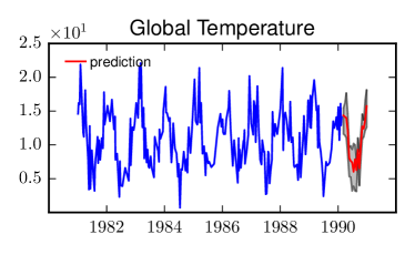
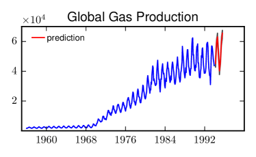
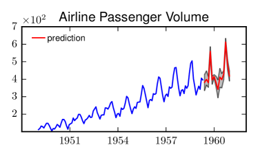
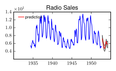
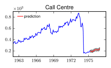
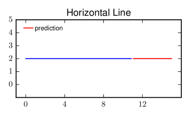
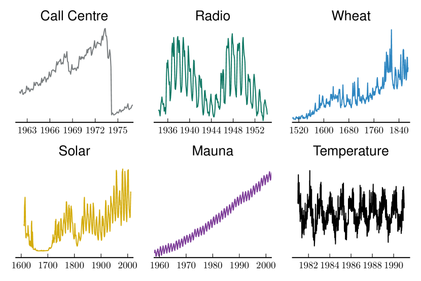
This set of benchmark problems consists of five real-world time series datasets from Lloyd 2014: (i) bi-weekly global temperature measurements from 1980 to 1990, (ii) monthly global gas production from 1956 to 1995, (iii) monthly airline passenger volume from 1948, (iv) monthly radio sales from 1935 to 1954, and (iv) monthly call center activity from 1962 to 1976. Each of the datasets has a different qualitative structure. For example, the global temperature dataset is comprised of yearly periodic structure overlaid with white noise, while the call center dataset has a linear trend until 1973 and a sharp drop afterwards. Figure 7 shows the five datasets, along with the inferences our technique made about the qualitative structure of the data generating process underlying each dataset. The results show that our technique accurately infers the presence or absence of each type of structure in each benchmark. Specifically, if a specific qualitative structure is deemed to be present if the posterior probability inferred by our technique is above 50%, and inferred to be absent otherwise, then the inferences from Bayesian synthesis match the real world structure in every case. To confirm that the synthesized programs report the absence of any meaningful structure when it is not present in the data, we also include a horizontal line shown in panel 1(f).

7.2. Quantitative Prediction Accuracy for Time Series Data

Figure 9 shows quantitative prediction accuracy for seven real world econometric time series. The top panel visually compares predictions from our method with predictions obtained by baseline methods on the airline passenger volume benchmark. We chose to compare against baselines that (i) have open source, re-usable implementations; (ii) are widely used and cited in the statistical literature; and (iii) are based on flexible model families that, like our Gaussian process technique, have default hyperparameter settings and do not require significant manual tuning to fit the data. Baseline methods include Facebook’s Prophet algorithm (Taylor and Letham 2018); standard econometric techniques, such as Auto-Regressive Integrated Moving Average (ARIMA) modeling (Hyndman and Khandakar 2008); and advanced time series modeling techniques from nonparametric Bayesian statistics, such as the Hierarchical Dirichlet Process Hidden Markov Model (Johnson and Willsky 2013). Bayesian synthesis is the only technique that accurately captures both quantitative and qualitative structure. The bottom panel of Figure 9 shows quantitative results comparing predictive accuracy on these datasets. Bayesian synthesis produces more accurate models for five of the seven benchmark problems and is competitive with other techniques on the other two problems.

7.3. Runtime Versus Prediction Accuracy for Time Series Data

(a) Runtime vs. Accuracy Profiles

(b) Time Series Datasets

Figure 10. Synthesis runtime versus held-out predictive likelihood on the time series benchmarked in Figure 9. Panel 10(a) shows a log-linear plot of the median runtime and predictive likelihood values taken over 100 independent runs of synthesis. Higher values of predictive likelihood on the y-axis indicate better fit to the observed data. Panel 10(b) shows the time series datasets used to compute runtime and accuracy measurements.

	Variable 1	Variable 2	True Predictive Structure		Predictive Relationship Detected By
					Pearson Correlation		Bayesian Synthesis
11(a)	flavanoids	color-intensity	linear + bimodal	$\checkmark$	$\times$	$(0.03)$	$\checkmark$	$(0.97)$
11(b)	A02	A07	linear + heteroskedastic	$\checkmark$	$\times$	$(0.16)$	$\checkmark$	$(0.89)$
11(c)	A02	A03	linear + bimodal + heteroskedastic	$\checkmark$	$\times$	$(0.03)$	$\times$	$(0.66)$
11(d)	proline	od280-of-wines	nonlinear + missing regime	$\checkmark$	$\times$	$(0.09)$	$\checkmark$	$(0.97)$
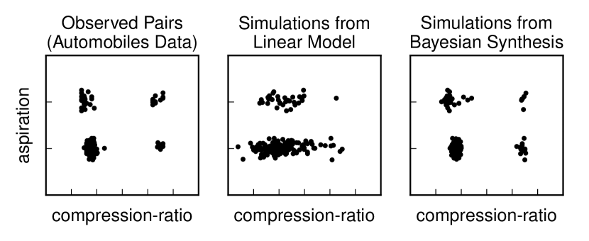
11(e)	compression-ratio	aspiration	mean shift	$\checkmark$	$\times$	$(0.07)$	$\checkmark$	$(0.98)$
11(f)	age	income	different group tails	$\checkmark$	$\times$	$(0.06)$	$\checkmark$	$(0.90)$
11(g)	age	varices	scale shift	$\checkmark$	$\times$	$(0.00)$	$\checkmark$	$(0.90)$
11(h)	capital-gain	income	different group tails	$\checkmark$	$\times$	$(0.05)$	$\times$	$(0.77)$
11(i)	city-mpg	highway-mpg	linearly increasing	$\checkmark$	$\checkmark$	$(0.95)$	$\checkmark$	$(1.00)$
11(j)	horsepower	highway-mpg	linearly decreasing	$\checkmark$	$\checkmark$	$(0.65)$	$\checkmark$	$(1.00)$
11(k)	education-years	education-level	different group means	$\checkmark$	$\checkmark$	$(1.00)$	$\checkmark$	$(1.00)$
11(l)	compression-ratio	fuel-type	different group means	$\checkmark$	$\checkmark$	$(0.97)$	$\checkmark$	$(0.98)$
11(m)	cholesterol	max-heart-rate	none (+ outliers)	$\times$	$\times$	$(0.00)$	$\times$	$(0.08)$
11(n)	cholesterol	st-depression	none (+ outliers)	$\times$	$\times$	$(0.00)$	$\times$	$(0.00)$
11(o)	blood-pressure	sex	none	$\times$	$\times$	$(0.01)$	$\times$	$(0.26)$
11(p)	st-depression	electrocardiography	none	$\times$	$\times$	$(0.04)$	$\times$	$(0.00)$

(a) Linear + Bimodal

(b) Linear + Heteroskedastic

(c) Bimodal + Heteroskedastic

(d) Missing Regime

(e) Mean Shift

(f) Scale Shift

(g) Different Tails

(h) Different Tails

(i) Linearly Increasing

(j) Linearly Decreasing

(k) Different Group Means

(l) Different Group Means

(m) No Dependence + Outliers

(n) No Dependence + Outliers

(o) No Dependence

(p) No Dependence

Figure 11. Detecting probable predictive relationships between pairs of variables for widely varying dependence structures including nonlinearity, heteroskedasticity, mean and scale shifts, and missing regimes. The table in the top panel shows 16 pairs of variables, the true predictive structure between them, and indicators as to whether a predictive relationship, if any, was detected by Pearson correlation and Bayesian synthesis.

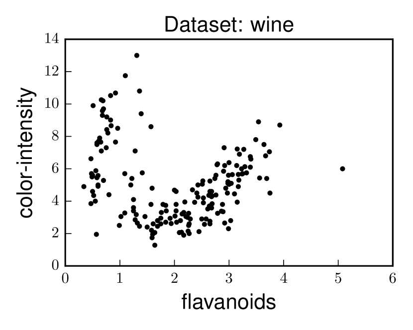
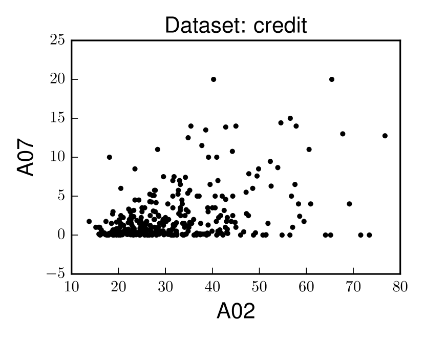
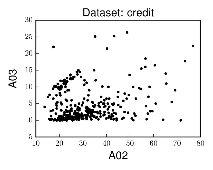
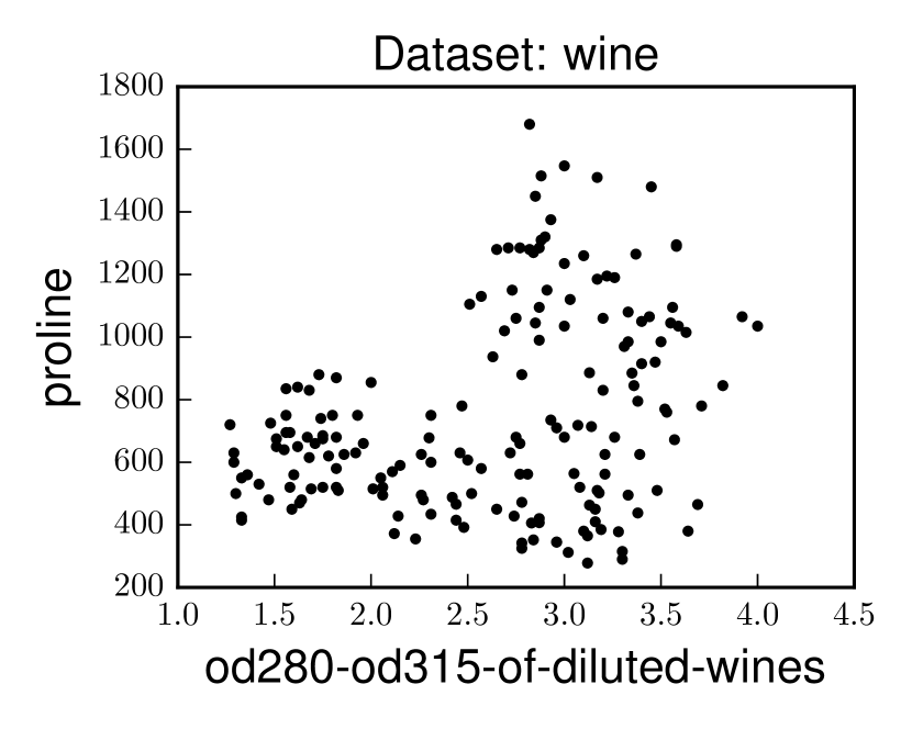
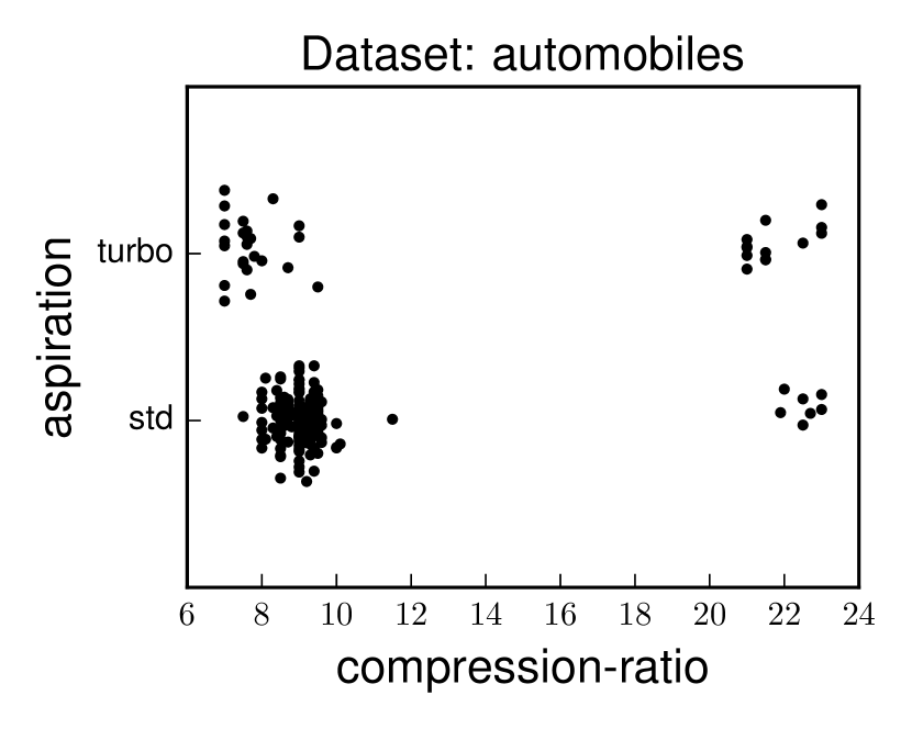
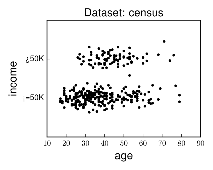
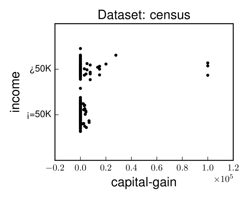
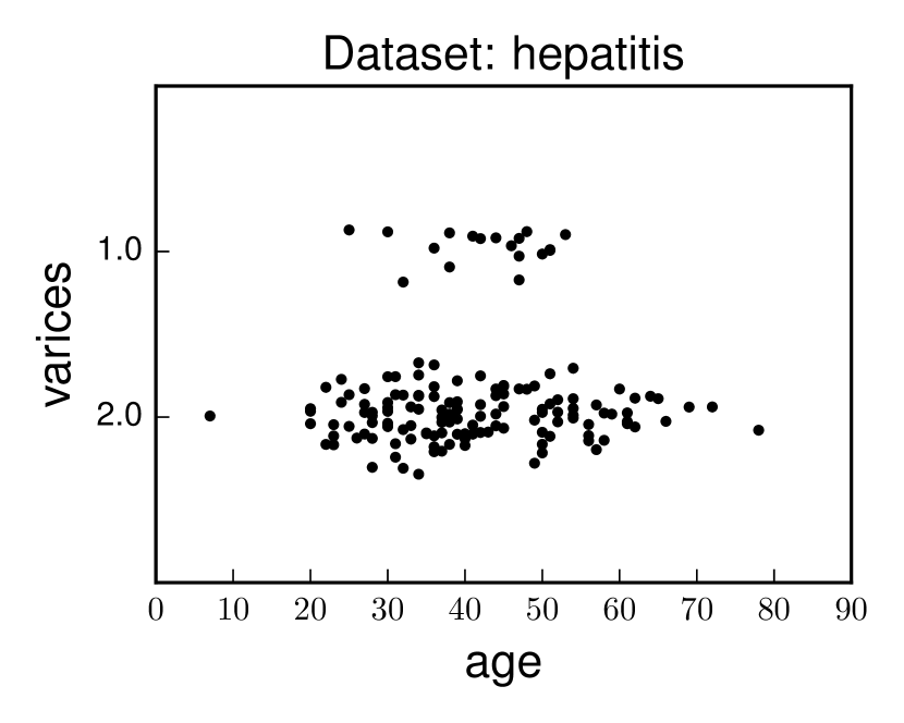
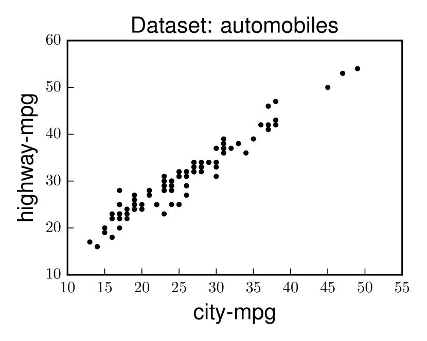
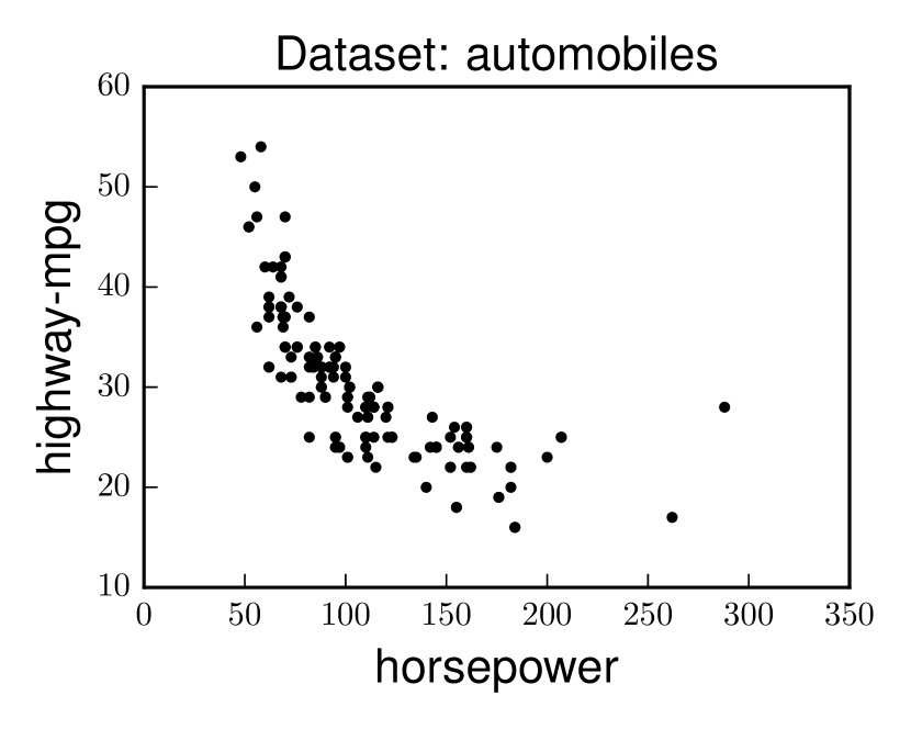
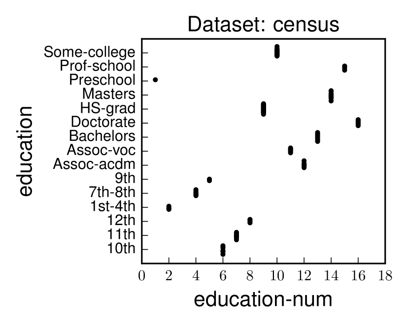
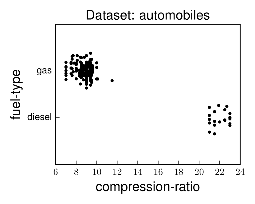
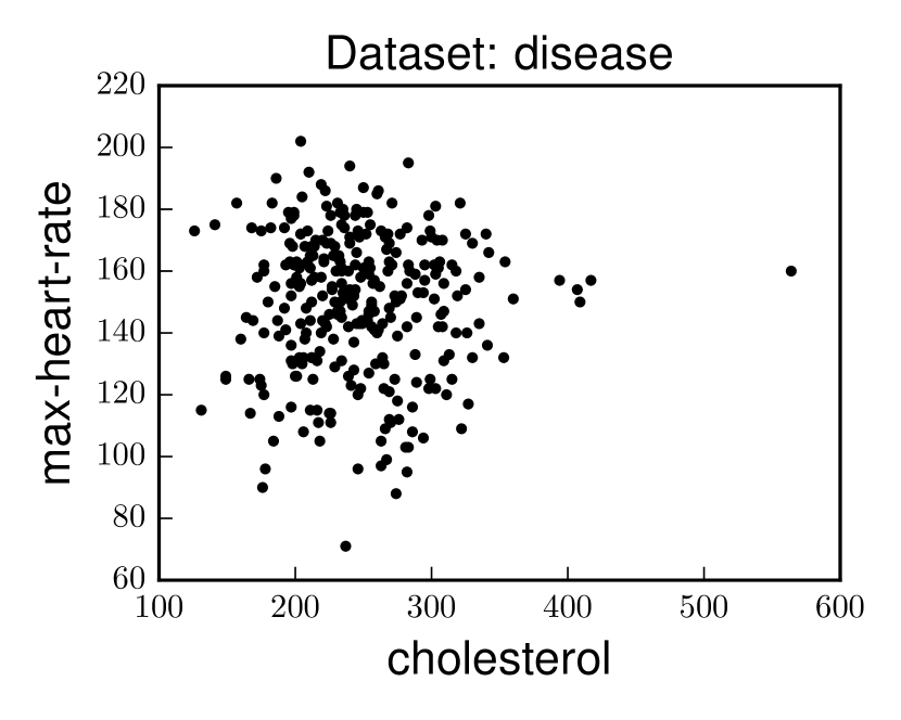
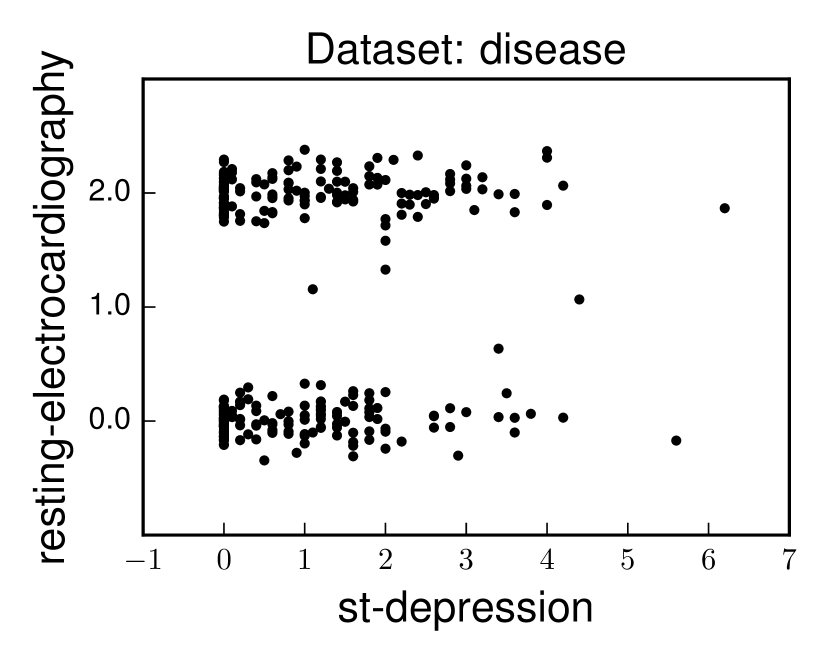
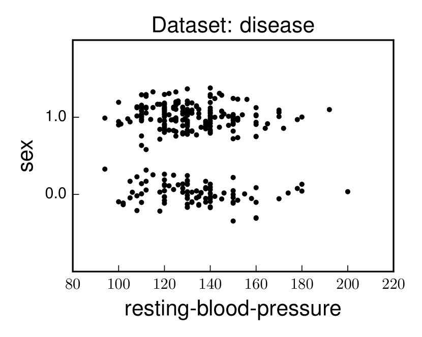
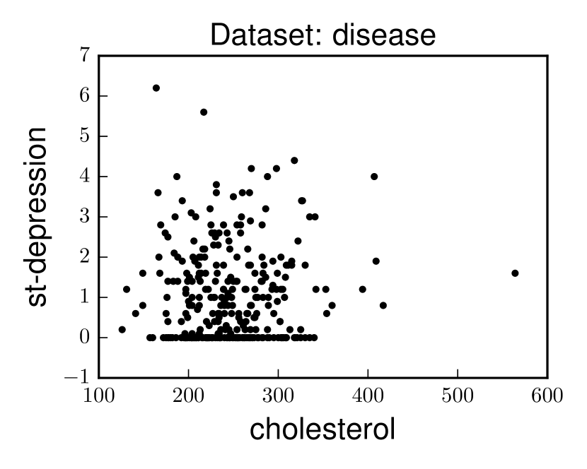
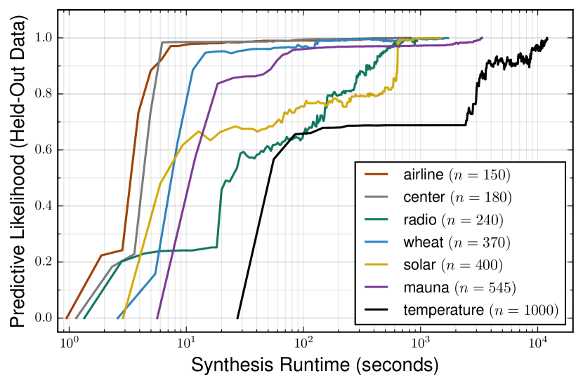
Figure 10 shows a profile of the predictive likelihood on held-out data versus the synthesis runtime (in seconds) for each of the seven econometric time series. For each dataset, we ran 2000 steps of synthesis, taking runtime and predictive likelihood measurements at every 5 steps. The plotted runtime and predictive likelihood values represent the median values taken over 100 independent runs of Bayesian synthesis for each dataset. The predictive likelihood measurements on the y-axis are scaled between 0 and 1 so that these profiles can be compared across the seven datasets. We see that there is significant variance in the synthesis runtime versus prediction quality. For certain time series such as airline and call datasets (150 and 180 observations), prediction quality stabilizes after around 10 seconds; for radio and solar datasets (240 and 400 observations) the prediction quality takes around 1000 seconds to stabilize; and for the temperature dataset (1000 observations) the predictions continue to improve even after exceeding the maximum timeout.

Recall from Section 5.1 that each step of synthesis has a time complexity of $O(l_{G}+|E|n^{2}+n^{3})$. Scaling the synthesis to handle time series with more than few thousands data points will require the sparse Gaussian process techniques discussed in Section 5.1. It is also important to emphasize that the time cost of each iteration of synthesis is not only a function of the number of observations $n$ but also the size $\lvert E\rvert$ of the synthesized programs. Thus, while more observations typically require more time, time series with more complex temporal patterns typically result in longer synthesized programs. This trade-off can be seen by comparing the profiles of the mauna data (545 observations) with the radio data (240 observations). While mauna has more observations $n$, the radio data contains much more complex periodic patterns and which requires comparatively longer programs and thus longer synthesis times.

7.4. Inferring Qualitative Structure from Multivariate Tabular Data

A central goal of data analysis for multivariate tabular data is to identify predictive relationships between pairs of variables (Ezekiel 1941; Draper and Smith 1966). Recall from Section 6 that synthesized programs from the multivariate tabular data DSL place related variables in the same variable block expression. Using Eq (5) from Section 3.1, we report a relationship between a pair of variables if 80% of the synthesized programs place these variables in the same block. We compare our method to the widely-used Pearson correlation baseline (Abbott 2016) by checking whether the correlation value exceeds 0.20 (at the $5\%$ significance level).

We evaluate the ability of our method to correctly detect related variables in six real-world datasets from the UCI machine learning repository (Dheeru and Karra Taniskidou 2017): automobile data (26 variables), wine data (14 variables), hepatitis data (20 variables), heart disease data (15 variables), and census data (15 variables). Figure 11 shows results for sixteen selected pairs of variables in these datasets (scatter plots shown in 11(a)–11(p)). Together, these pairs exhibit a broad class of relationships, including linear, nonlinear, heteroskedastic, and multi-modal patterns. Four of the benchmarks, shown in the final row, have no predictive relationship.

(a) Bimodal Dependence

(b) Bimodal Increasing Linear Dependence

 

(c) Heavy-Tailed Nonlinear Dependence

(d) Missing Regime Nonlinear Dependence

Figure 12. Comparing the quality of predictive models discovered by Bayesian synthesis to commonly-used generalized linear models, for several real-world datasets and dependence patterns. In each of the panels 12(a)–12(d), the first column shows a scatter plot of two variables in the observed dataset; the second column shows data simulated from a linear model trained on the observed data; and the third column shows data simulated from probabilistic programs obtained using Bayesian synthesis given the observed data. The synthesized programs are able to detect underlying patterns and emulate the true distribution, including nonlinear, multi-modal, and heteroskedastic relationships. Simulations from linear models have a poor fit.

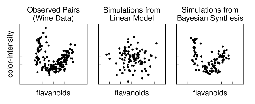
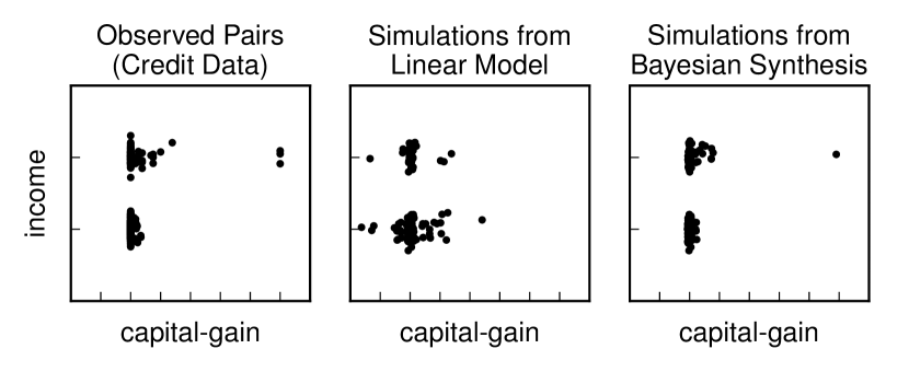
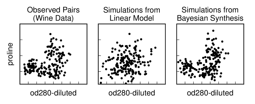
The table in Figure 11 shows that our method correctly detects the presence or absence of a predictive relationship in 14 out of 16 benchmarks, where the final column shows the posterior probability of a relationship in each case. In contrast, Pearson correlation, shown in the second-to-last column, only obtains the correct answer in 8 of 16 benchmarks. This baseline yields incorrect answers for all pairs of variables with nonlinear, bimodal, and/or heteroskedastic relationships. These results show that Bayesian synthesis provides a practical method for detecting complex predictive relationships from real-world data that are missed by standard baselines.

Moreover, Figure 12 shows that probabilistic programs from Bayesian synthesis are able to generate entirely new datasets that reflect the pattern of the predictive relationship in the underlying data generating process more accurately than generalized linear statistical models.

(a) Median Error in Predictive Log-Likelihood of Held-Out Data

Benchmark	Kernel Density Estimation	Bayesian Synthesis
biasedtugwar	$-1.58\text{\times}{10}^{-01}$	$-3.13\text{\times}{10}^{-02}$
burglary	$-4.25\text{\times}{10}^{-01}$	$-1.45\text{\times}{10}^{-03}$
csi	$-1.00\text{\times}{10}^{-01}$	$-4.35\text{\times}{10}^{-04}$
easytugwar	$-2.96\text{\times}{10}^{-01}$	$-9.96\text{\times}{10}^{-02}$
eyecolor	$-4.69\text{\times}{10}^{-02}$	$-5.31\text{\times}{10}^{-03}$
grass	$-3.91\text{\times}{10}^{-01}$	$-4.49\text{\times}{10}^{-02}$
healthiness	$-1.35\text{\times}{10}^{-01}$	$-3.00\text{\times}{10}^{-03}$
hurricane	$-1.30\text{\times}{10}^{-01}$	$-2.11\text{\times}{10}^{-04}$
icecream	$-1.51\text{\times}{10}^{-01}$	$-7.07\text{\times}{10}^{-02}$
mixedCondition	$-1.06\text{\times}{10}^{-01}$	$-1.43\text{\times}{10}^{-02}$
multipleBranches	$-4.12\text{\times}{10}^{-02}$	$-1.22\text{\times}{10}^{-02}$
students	$-1.74\text{\times}{10}^{-01}$	$-5.47\text{\times}{10}^{-02}$
tugwarAddition	$-2.60\text{\times}{10}^{-01}$	$-1.38\text{\times}{10}^{-01}$
uniform	$-2.72\text{\times}{10}^{-01}$	$-1.26\text{\times}{10}^{-01}$

Figure 13. Comparing the error in the predictive probabilities of held-out data according to Bayesian synthesis and KDE. For each of the 13 benchmark problems, a training set of 10,000 data records was used to synthesize probabilistic programs in our tabular data DSL and to fit KDE models. 10,000 new data records were then used to assess held-out predictive probabilities, which measures how well the synthesized probabilistic programs are able to model the true distribution. The scatter plots on the right show the full distribution of the true (log) probabilities (according to the ground-truth program) and the predictive probabilities (according to the synthesized programs) for six of the benchmarks (each red dot is a held-out data record). Estimates are most accurate and certain in the bulk of the distribution and are less accurate and less certain in the tails.

7.5. Quantitative Prediction Accuracy for Multivariate Tabular Data

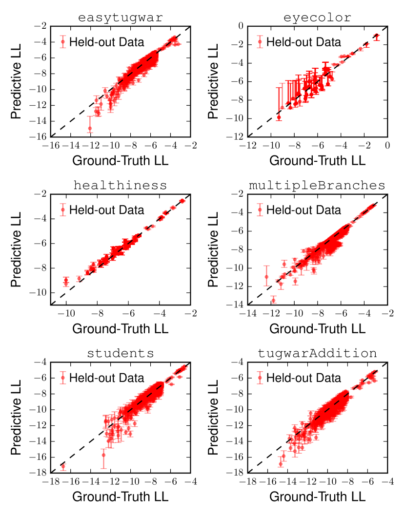
Another central goal of data analysis for multivariate tabular data is to learn probabilistic models that can accurately predict the probability of new data records, a task known as density estimation (Silverman 1986; Scott 2009). Accurately predicting the probability of new data enables several important tasks such as data cleaning, anomaly detection, and imputing missing data. We obtain the probability of new data records according to the synthesized probabilistic programs by first translating the programs into Venture (right column of Figure 5) and then executing the translated programs in the Venture inference environment. Given a new data record, these programs immediately return the probability of the new data record according to the probabilistic model specified by the Venture probabilistic program. We compare our method to the widely-used multivariate kernel density estimation (KDE) baseline with mixed data types from Racine and Li 2004.

We evaluate our method’s ability to accurately perform density estimation using 13 benchmark datasets adapted from Chasins and Phothilimthana 2017. Each dataset was generated by a “ground-truth” probabilistic program written in BLOG (Milch et al. 2005). Because the ground-truth program is available, we can compare the actual probability of each new data record (obtained from the ground-truth BLOG program) with its predicted probability (obtained from the synthesized Venture programs and from KDE). The results in the table in Figure 13 show that our method is more accurate than KDE, often by several orders of magnitude. A key advantage of our approach is that we synthesize an ensemble of probabilistic programs for each dataset. This ensemble enables us to approximate the full posterior distribution and then use this distribution to compute error bars for predicted probability values. The scatter plots in Figure 13 show that the error bars are well-calibrated, i.e. error bars are wider for data records where our method gives less accurate estimates. In contrast, KDE only gives point estimates with no error bars and no measure of uncertainty.

8. Related Work

We discuss related work in five related fields: Bayesian synthesis of probabilistic programs (where this work is the first), non-Bayesian synthesis of probabilistic programs, probabilistic synthesis of non-probabilistic programs, non-probabilistic synthesis of non-probabilistic programs, and model discovery in probabilistic machine learning.

Bayesian synthesis of probabilistic programs. This paper presents the first Bayesian synthesis of probabilistic programs. It presents the first formalization of Bayesian synthesis for probabilistic programs and the first soundness proofs of Bayesian synthesis for probabilistic programs generated by probabilistic context-free grammars. It also presents the first empirical demonstration of accurate modeling of multiple real-world domains and tasks via this approach.

This paper is also the first to: (i) identify sufficient conditions to obtain a well-defined posterior distribution; (ii) identify sufficient conditions to obtain a sound Bayesian synthesis algorithm; (iii) define a general family of domain-specific languages with associated semantics that ensure that the required prior and posterior distributions are well-defined; (iv) present a sound synthesis algorithm that applies to any language in this class of domain-specific languages; and (v) present a specific domain-specific language (the Gaussian process language for modeling time series data) that satisfies these sufficient conditions.

Nori et al. 2015 introduce a system (PSKETCH) designed to complete partial sketches of probabilistic programs for modeling tabular data. The technique is based on applying sequences of program mutations to a base program written in a probabilistic sketching language. As we detail further below, the paper uses the vocabulary of Bayesian synthesis to describe the technique but contains multiple fundamental technical errors that effectively nullify its key claims. Specifically, Nori et al. 2015 proposes to use Metropolis-Hastings sampling to approximate the maximum a posteriori solution to the sketching problem. However, the paper does not establish that the prior or posterior distributions on programs are well-defined. The paper attempts to use a uniform prior distribution over an unbounded space of programs. However, there is no valid uniform probability measure over this space. Because the posterior is defined using the prior and the marginal likelihood of all datasets is not shown to be finite, the posterior is also not well-defined. The paper presents no evidence or argument that the proposed prior or posterior distribution is well-defined. The paper also asserts that the synthesis algorithm converges because the MH algorithm always converges, but it does not establish that the presented framework satisfies the properties required for the MH algorithm to converge. And because the posterior is not well-defined, there is no probability distribution to which the MH algorithm can converge. We further note that while the paper claims to use the MH algorithm to determine whether a proposed program mutation is accepted or rejected, there is in fact no tractable algorithm that can be used to compute the reversal probability of going back from a proposed to an existing program, which means the MH algorithm cannot possibly be used with the program mutation proposals described in the paper.

The presented system, PSKETCH, is based on applying sequences of program mutations to a base program written in a probabilistic sketching language with constructs (such as if-then-else, for loops, variable assignment, and arbitrary arithmetic operations) drawn from general-purpose programming languages. We believe that, consistent with the experimental results presented in the paper, working only with these constructs is counterproductive in that it produces a search space that is far too unconstrained to yield practical solutions to real-world data modeling problems in the absence of other sources of information that can more effectively narrow the search. We therefore predict that the field will turn to focus on probabilistic DSLs (such as the ones presented in this paper) as a way to more effectively target the problems that arise in automatic data modeling. As an example, while the sketching language in Nori et al. 2015 contains general-purpose programming constructs, it does not have domain-specific constructs that concisely represent Gaussian processes, covariance functions, or rich nonparametric mixture models used in this paper.

Hwang et al. 2011 use beam search over arbitrary program text in a subset of the Church (Goodman et al. 2008) language to obtain a generative model over tree-like expressions. The resulting search space is so unconstrained that, as the authors note in the conclusion, this technique does not apply to any real-world problem whatsoever. This drawback highlights the benefit of controlling the search space via an appropriate domain-specific language. In addition we note that although Hwang et al. 2011 also use the vocabulary of Bayesian synthesis, the proposed program-length prior over an unbounded program space is not shown to be probabilistically well-formed, nor is it shown to lead to a valid Bayesian posterior distribution over programs, nor is the stochastic approximation of the program likelihood shown to result in a sound synthesis algorithm.

Non-Bayesian synthesis of probabilistic programs. Ellis et al. 2015 introduce a method for synthesizing probabilistic programs by using SMT solvers to optimize the likelihood of the observed data with a regularization term that penalizes the program length. The research works with a domain-specific language for morphological rule learning. Perov and Wood 2014 propose to synthesize code for simple random number generators using approximate Bayesian computation. These two techniques are fundamentally different from ours. They focus on different problems, specifically morphological rule learning, visual concept learning, and random number generators, as opposed to data modeling. Neither is based on Bayesian learning and neither presents soundness proofs (or even states a soundness property). Moreover, both attempt to find a single highest-scoring program as opposed to synthesizing ensembles of programs that approximate a Bayesian posterior distribution over the sampled probabilistic programs. As this previous research demonstrates, obtaining soundness proofs or characterizing the uncertainty of the synthesized programs against the data generating process is particularly challenging for non-Bayesian approaches because of the ad-hoc nature of the synthesis formulation.

Tong and Choi 2016 describe a method which uses an off-the-shelf model discovery system (Lloyd 2014, ABCD) to learn Gaussian process models and the code-generate the models to Stan (Carpenter et al. 2017) programs. However, Tong and Choi 2016 does not formalize the program synthesis problem, nor does it present any formal semantics, nor does it show how to extract the probability that qualitative properties hold in the data, nor does it apply to multiple model families in a single problem domain let alone multiple problem domains. Chasins and Phothilimthana 2017 present a technique for synthesizing probabilistic programs in tabular datasets using if-else statements. Unlike our method, their approach requires the user to manually specify a causal ordering between the variables. This information may be difficult or impossible to obtain. Second, the proposed technique is based on using linear correlation, which we have shown in our experiments (Figures 12 and 11) fails to adequately capture complex probabilistic relationships. Finally, the paper is based on simulated annealing, not Bayesian synthesis, has no probabilistic interpretation, and does not claim to provide a notion of soundness.

Probabilistic synthesis of non-probabilistic programs. Schkufza et al. 2013 describe a technique for synthesizing high-performance X86 binaries by using MCMC to stochastically search through a space of programs and to deliver a single X86 program which satisfies the hard constraint of correctness and the soft constraint of performance improvement. While both the Bayesian synthesis framework in this paper and the superoptimization technique from Schkufza et al. 2013 use MCMC algorithms to implement the synthesis, they use MCMC in a fundamentally different way. In Schkufza et al. 2013, MCMC is used as a strategy to search through a space of deterministic programs that seek to minimize a cost function that itself has no probabilistic semantics. In contrast, Bayesian synthesis uses MCMC as a strategy to approximately sample from a space of probabilistic programs whose semantics specify a well-defined posterior distribution programs.

Bayesian priors over structured program representations which seek to sample from a posterior distribution over programs have also been investigated. Liang et al. 2010 use adapter grammars (Johnson et al. 2007) to build a hierarchical nonparametric Bayesian prior over programs specified in combinatory logic (Schönfinkel 1924). Ellis et al. 2016 describe a method to sample from a bounded program space with a uniform prior where the posterior probability of a program is equal to (i) zero if it does not satisfy an observed input-output constraint, or (ii) geometrically decreasing in its length otherwise. These methods are used to synthesize arithmetic operations, text editing, and list manipulation programs. Both Liang et al. 2010 and Ellis et al. 2015 specify Bayesian priors over programs similar to the prior in this paper. However, these two techniques are founded on the assumption that the synthesized programs have deterministic input-output behavior and cannot be easily extended to synthesize programs that have probabilistic input-output behavior. In contrast, the Bayesian synthesis framework presented in this paper can synthesize programs with deterministic input-output behavior by adding hard constraints to the $\mathsf{Lik}$ semantic function, although alternative synthesis techniques may be required to make the synthesis more effective.

Lee et al. 2018 present a technique for speeding up program synthesis of non-probabilistic programs by using A* search to enumerate programs that satisfy a set of input-output constraints in order of decreasing prior probability. This prior distribution over programs is itself learned using a probabilistic higher-order grammar with transfer learning over a large corpus of existing synthesis problems and solutions. The technique is used to synthesize programs in domain-specific languages for bit-vector, circuit, and string manipulation tasks. Similar to the Bayesian synthesis framework in this paper, Lee et al. 2018 use PCFG priors for specifying domain-specific languages. However the fundamental differences are that the synthesized programs in Lee et al. 2018 are non-probabilistic and the objective is to enumerate valid programs sorted by their prior probability, while in this paper the synthesized programs are probabilistic so enumeration is impossible and the objective is instead to sample programs according to their posterior probabilities.

Non-probabilistic synthesis of non-probabilistic programs. Over the last decade program synthesis has become a highly active area of research in programming languages. Key techniques include deductive logic with program transformations (Burstall and Darlington 1977; Manna and Waldinger 1979; Manna and Waldinger 1980), genetic programming (Koza 1992; Koza et al. 1997), solver and constraint-based methods (Solar-Lezama et al. 2006; Jha et al. 2010; Gulwani et al. 2011; Gulwani 2011; Feser et al. 2015), syntax-guided synthesis (Alur et al. 2013), and neural networks (Graves et al. 2014; Reed and de Freitas 2016; Balog et al. 2017; Bošnak et al. 2018). In general these approaches have tended to focus on areas where uncertainty is not essential or even relevant to the problem being solved. In particular, synthesis tasks in this field apply to programs that exhibit deterministic input-output behavior in discrete problem domains with combinatorial solutions. There typically exists an “optimal” solution and the synthesis goal is to obtain a good approximation to this solution.

In contrast, in Bayesian synthesis the problem domain is fundamentally about automatically learning models of non-deterministic data generating processes given a set of noisy observations. Given this key characteristic of the problem domain, we deliver solutions that capture uncertainty at two levels. First, our synthesis produces probabilistic programs that exhibit noisy, non-deterministic input-output behavior. Second, our technique captures inferential uncertainty over the structure and parameters of the synthesized programs themselves by producing an ensemble of probabilistic programs whose varying properties reflect this uncertainty.

Model discovery in probabilistic machine learning. Researchers have developed several probabilistic techniques for discovering statistical model structures from observed data. Prominent examples include Bayesian network structures (Mansinghka et al. 2006), matrix-composition models (Grosse et al. 2012), univariate time series (Duvenaud et al. 2013), multivariate time series (Saad and Mansinghka 2018), and multivariate data tables (Mansinghka et al. 2016).

Our paper introduces a general formalism that explains and extends these modeling techniques. First, it establishes general conditions for Bayesian synthesis to be well-defined and introduces sound Bayesian synthesis algorithms that apply to a broad class of domain-specific languages.

Second, we show how to estimate the probability that qualitative structures are present or absent in the data. This capability rests on a distinctive aspect of our formalism, namely that soundness is defined in terms of sampling programs from a distribution that converges to the Bayesian posterior, not just finding a single “highest scoring” program. As a result, performing Bayesian synthesis multiple times yields a collection of programs that can be collectively analyzed to form Monte Carlo estimates of posterior and predictive probabilities.

Third, our framework shows one way to leverage probabilistic programming languages to simplify the implementation of model discovery techniques. Specifically, it shows how to translate programs in a domain-specific language into a general-purpose language such as Venture, so that the built-in language constructs for predictive inference can be applied (rather than requiring new custom prediction code for each model family). A key advantage of this approach is that representing probabilistic models as synthesized probabilistic programs enable a wide set of capabilities for data analysis tasks (Saad and Mansinghka 2016; Saad and Mansinghka 2017).

Fourth, we implemented two examples of domain-specific languages and empirically demonstrate accuracy improvements over multiple baselines.

9. Conclusion

We present a technique for Bayesian synthesis of probabilistic programs for automatic data modeling. This technique enables, for the first time, users to solve important data analysis problems without manually writing statistical programs or probabilistic programs. Our technique (i) produces an ensemble of probabilistic programs that soundly approximate the Bayesian posterior, allowing an accurate reflection of uncertainty in predictions made by the programs; (ii) is based on domain-specific modeling languages that are empirically shown to capture the qualitative structure of a broad class of data generating processes; (iii) processes synthesized programs to extract qualitative structures from the surface syntax of the learned programs; (iv) translates synthesized programs into probabilistic programs that provide the inference machinery needed to obtain accurate predictions; and (v) is empirically shown to outperform baseline statistical techniques for multiple qualitative and quantitative data analysis and prediction problems.

Designing good probabilistic domain-specific languages and priors is a key characteristic of our approach to automatic data modeling. In this paper we focus on broad non-parametric Bayesian priors that are flexible enough to capture a wide range of patterns and are also tractable enough for Bayesian synthesis. In effect, the choice of prior is embedded in the language design pattern, is done once when the language is designed, and can be reused across applications. The high-level nature of the DSL and carefully designed priors allow us to restrict the space of probabilistic programs to those that are well-suited for a particular data modeling task (such as time series and multivariate data tables). Once an appropriate DSL is developed, the synthesis algorithms can then be optimized on a per-DSL basis. Future directions of research include developing optimized synthesis algorithms to improve scalability; adding language support for user-specified qualitative constraints that must hold in the synthesized programs; and information-flow analyses on the synthesized programs to quantify relationships between variables in the underlying data generating process.

Appendix A Proofs for Gaussian Process Domain-Specific Language

Section 5 of the main text states that the prior and likelihood semantics of the Gaussian process domain-specific language satisfy the theoretical preconditions required for Bayesian synthesis. In particular, we prove the following lemma:

Lemma A.1.

The $\mathsf{Prior}$ and $\mathsf{Lik}$ semantic functions in Figure 4 satisfy Conditions 3.1, 3.2, and 3.3.

Proof for Condition 3.1.

Letting upper-case symbols denote non-terminals $N$ and lower-case words in teletype denote terminals, the equivalent context-free grammar in Chomsky normal form is given by:

$$K \to CB_{[0.14]}\mid EB_{[0.14]}\mid GB_{[0.14]}\mid IB_{[0.14]}\mid PB_{[0.14]}\mid TM_{[0.135]}\mid VM_{[0.135]}\mid WX_{[0.03]}$$

$$C \to\texttt{const}$$

$$E \to\texttt{wn}$$

$$G \to\texttt{lin}$$

$$I \to\texttt{se}$$

$$P \to\texttt{per}$$

$$B \to\texttt{gamma}$$

$$T \to\texttt{+}$$

$$V \to\texttt{*}$$

$$W \to\texttt{cp}$$

$$M \to KK$$

$$X \to BM,$$

where subscripts indicate the production probabilities for non-terminals with more than one production rule . Following the notation from Gecse and Kovács 2010, define:

$$m_{ij} =\textstyle\sum_{k=1}^{r_{i}}p_{ik}n_{ikj} (i,j=1,\dots,n)$$

where

$$r_{i} :\mbox{ number of productions with }N_{i}\in N\mbox{ premise},$$

$$p_{ik} :\mbox{ probability assigned to production }k\mbox{ of }N_{i},$$

$$n_{ikj} :\mbox{ number of occurrence of }N_{j}\in N\mbox{ in production }k\mbox{ of }N_{i}.$$

The expectation matrix $M\Coloneqq[m_{ij}]$ is given by:

$$\hbox{}\vbox{\kern 0.86108pt\hbox{$\kern 0.0pt\kern 2.5pt\kern-5.0pt\left[\kern 0.0pt\kern-2.5pt\kern-5.55557pt\vbox{\kern-0.86108pt\vbox{\vbox{\halign{\kern\arraycolsep\hfil\@arstrut$\kbcolstyle#$\hfil\kern\arraycolsep& \kern\arraycolsep\hfil$\@kbrowstyle#$\ifkbalignright\relax\else\hfil\fi\kern\arraycolsep&& \kern\arraycolsep\hfil$\@kbrowstyle#$\ifkbalignright\relax\else\hfil\fi\kern\arraycolsep\cr 5.0pt\hfil\hbox{\vrule height=0.0pt,depth=0.0pt,width=0.0pt}$\scriptstyle$\hfil\kern 5.0pt&5.0pt\hfil$\scriptstyle K$\hfil\kern 5.0pt&5.0pt\hfil$\scriptstyle C$\hfil\kern 5.0pt&5.0pt\hfil$\scriptstyle E$\hfil\kern 5.0pt&5.0pt\hfil$\scriptstyle G$\hfil\kern 5.0pt&5.0pt\hfil$\scriptstyle I$\hfil\kern 5.0pt&5.0pt\hfil$\scriptstyle P$\hfil\kern 5.0pt&5.0pt\hfil$\scriptstyle B$\hfil\kern 5.0pt&5.0pt\hfil$\scriptstyle T$\hfil\kern 5.0pt&5.0pt\hfil$\scriptstyle V$\hfil\kern 5.0pt&5.0pt\hfil$\scriptstyle W$\hfil\kern 5.0pt&5.0pt\hfil$\scriptstyle M$\hfil\kern 5.0pt&5.0pt\hfil$\scriptstyle X$\hfil\kern 5.0pt\\ 5.0pt\hfil\hbox{\vrule height=0.0pt,depth=0.0pt,width=0.0pt}$\scriptstyle K$\hfil\kern 5.0pt&5.0pt\hfil$\scriptstyle 0$\hfil\kern 5.0pt&5.0pt\hfil$\scriptstyle 0.14$\hfil\kern 5.0pt&5.0pt\hfil$\scriptstyle 0.14$\hfil\kern 5.0pt&5.0pt\hfil$\scriptstyle 0.14$\hfil\kern 5.0pt&5.0pt\hfil$\scriptstyle 0.14$\hfil\kern 5.0pt&5.0pt\hfil$\scriptstyle 0.14$\hfil\kern 5.0pt&5.0pt\hfil$\scriptstyle 0.70$\hfil\kern 5.0pt&5.0pt\hfil$\scriptstyle 0.135$\hfil\kern 5.0pt&5.0pt\hfil$\scriptstyle 0.135$\hfil\kern 5.0pt&5.0pt\hfil$\scriptstyle 0.03$\hfil\kern 5.0pt&5.0pt\hfil$\scriptstyle 0.27$\hfil\kern 5.0pt&5.0pt\hfil$\scriptstyle 0.03$\hfil\kern 5.0pt\\ 5.0pt\hfil\hbox{\vrule height=0.0pt,depth=0.0pt,width=0.0pt}$\scriptstyle C$\hfil\kern 5.0pt&5.0pt\hfil$\scriptstyle 0$\hfil\kern 5.0pt&5.0pt\hfil$\scriptstyle 0$\hfil\kern 5.0pt&5.0pt\hfil$\scriptstyle 0$\hfil\kern 5.0pt&5.0pt\hfil$\scriptstyle 0$\hfil\kern 5.0pt&5.0pt\hfil$\scriptstyle 0$\hfil\kern 5.0pt&5.0pt\hfil$\scriptstyle 0$\hfil\kern 5.0pt&5.0pt\hfil$\scriptstyle 0$\hfil\kern 5.0pt&5.0pt\hfil$\scriptstyle 0$\hfil\kern 5.0pt&5.0pt\hfil$\scriptstyle 0$\hfil\kern 5.0pt&5.0pt\hfil$\scriptstyle 0$\hfil\kern 5.0pt&5.0pt\hfil$\scriptstyle 0$\hfil\kern 5.0pt&5.0pt\hfil$\scriptstyle 0$\hfil\kern 5.0pt\\ 5.0pt\hfil\hbox{\vrule height=0.0pt,depth=0.0pt,width=0.0pt}$\scriptstyle E$\hfil\kern 5.0pt&5.0pt\hfil$\scriptstyle 0$\hfil\kern 5.0pt&5.0pt\hfil$\scriptstyle 0$\hfil\kern 5.0pt&5.0pt\hfil$\scriptstyle 0$\hfil\kern 5.0pt&5.0pt\hfil$\scriptstyle 0$\hfil\kern 5.0pt&5.0pt\hfil$\scriptstyle 0$\hfil\kern 5.0pt&5.0pt\hfil$\scriptstyle 0$\hfil\kern 5.0pt&5.0pt\hfil$\scriptstyle 0$\hfil\kern 5.0pt&5.0pt\hfil$\scriptstyle 0$\hfil\kern 5.0pt&5.0pt\hfil$\scriptstyle 0$\hfil\kern 5.0pt&5.0pt\hfil$\scriptstyle 0$\hfil\kern 5.0pt&5.0pt\hfil$\scriptstyle 0$\hfil\kern 5.0pt&5.0pt\hfil$\scriptstyle 0$\hfil\kern 5.0pt\\ 5.0pt\hfil\hbox{\vrule height=0.0pt,depth=0.0pt,width=0.0pt}$\scriptstyle G$\hfil\kern 5.0pt&5.0pt\hfil$\scriptstyle 0$\hfil\kern 5.0pt&5.0pt\hfil$\scriptstyle 0$\hfil\kern 5.0pt&5.0pt\hfil$\scriptstyle 0$\hfil\kern 5.0pt&5.0pt\hfil$\scriptstyle 0$\hfil\kern 5.0pt&5.0pt\hfil$\scriptstyle 0$\hfil\kern 5.0pt&5.0pt\hfil$\scriptstyle 0$\hfil\kern 5.0pt&5.0pt\hfil$\scriptstyle 0$\hfil\kern 5.0pt&5.0pt\hfil$\scriptstyle 0$\hfil\kern 5.0pt&5.0pt\hfil$\scriptstyle 0$\hfil\kern 5.0pt&5.0pt\hfil$\scriptstyle 0$\hfil\kern 5.0pt&5.0pt\hfil$\scriptstyle 0$\hfil\kern 5.0pt&5.0pt\hfil$\scriptstyle 0$\hfil\kern 5.0pt\\ 5.0pt\hfil\hbox{\vrule height=0.0pt,depth=0.0pt,width=0.0pt}$\scriptstyle I$\hfil\kern 5.0pt&5.0pt\hfil$\scriptstyle 0$\hfil\kern 5.0pt&5.0pt\hfil$\scriptstyle 0$\hfil\kern 5.0pt&5.0pt\hfil$\scriptstyle 0$\hfil\kern 5.0pt&5.0pt\hfil$\scriptstyle 0$\hfil\kern 5.0pt&5.0pt\hfil$\scriptstyle 0$\hfil\kern 5.0pt&5.0pt\hfil$\scriptstyle 0$\hfil\kern 5.0pt&5.0pt\hfil$\scriptstyle 0$\hfil\kern 5.0pt&5.0pt\hfil$\scriptstyle 0$\hfil\kern 5.0pt&5.0pt\hfil$\scriptstyle 0$\hfil\kern 5.0pt&5.0pt\hfil$\scriptstyle 0$\hfil\kern 5.0pt&5.0pt\hfil$\scriptstyle 0$\hfil\kern 5.0pt&5.0pt\hfil$\scriptstyle 0$\hfil\kern 5.0pt\\ 5.0pt\hfil\hbox{\vrule height=0.0pt,depth=0.0pt,width=0.0pt}$\scriptstyle P$\hfil\kern 5.0pt&5.0pt\hfil$\scriptstyle 0$\hfil\kern 5.0pt&5.0pt\hfil$\scriptstyle 0$\hfil\kern 5.0pt&5.0pt\hfil$\scriptstyle 0$\hfil\kern 5.0pt&5.0pt\hfil$\scriptstyle 0$\hfil\kern 5.0pt&5.0pt\hfil$\scriptstyle 0$\hfil\kern 5.0pt&5.0pt\hfil$\scriptstyle 0$\hfil\kern 5.0pt&5.0pt\hfil$\scriptstyle 0$\hfil\kern 5.0pt&5.0pt\hfil$\scriptstyle 0$\hfil\kern 5.0pt&5.0pt\hfil$\scriptstyle 0$\hfil\kern 5.0pt&5.0pt\hfil$\scriptstyle 0$\hfil\kern 5.0pt&5.0pt\hfil$\scriptstyle 0$\hfil\kern 5.0pt&5.0pt\hfil$\scriptstyle 0$\hfil\kern 5.0pt\\ 5.0pt\hfil\hbox{\vrule height=0.0pt,depth=0.0pt,width=0.0pt}$\scriptstyle B$\hfil\kern 5.0pt&5.0pt\hfil$\scriptstyle 0$\hfil\kern 5.0pt&5.0pt\hfil$\scriptstyle 0$\hfil\kern 5.0pt&5.0pt\hfil$\scriptstyle 0$\hfil\kern 5.0pt&5.0pt\hfil$\scriptstyle 0$\hfil\kern 5.0pt&5.0pt\hfil$\scriptstyle 0$\hfil\kern 5.0pt&5.0pt\hfil$\scriptstyle 0$\hfil\kern 5.0pt&5.0pt\hfil$\scriptstyle 0$\hfil\kern 5.0pt&5.0pt\hfil$\scriptstyle 0$\hfil\kern 5.0pt&5.0pt\hfil$\scriptstyle 0$\hfil\kern 5.0pt&5.0pt\hfil$\scriptstyle 0$\hfil\kern 5.0pt&5.0pt\hfil$\scriptstyle 0$\hfil\kern 5.0pt&5.0pt\hfil$\scriptstyle 0$\hfil\kern 5.0pt\\ 5.0pt\hfil\hbox{\vrule height=0.0pt,depth=0.0pt,width=0.0pt}$\scriptstyle T$\hfil\kern 5.0pt&5.0pt\hfil$\scriptstyle 0$\hfil\kern 5.0pt&5.0pt\hfil$\scriptstyle 0$\hfil\kern 5.0pt&5.0pt\hfil$\scriptstyle 0$\hfil\kern 5.0pt&5.0pt\hfil$\scriptstyle 0$\hfil\kern 5.0pt&5.0pt\hfil$\scriptstyle 0$\hfil\kern 5.0pt&5.0pt\hfil$\scriptstyle 0$\hfil\kern 5.0pt&5.0pt\hfil$\scriptstyle 0$\hfil\kern 5.0pt&5.0pt\hfil$\scriptstyle 0$\hfil\kern 5.0pt&5.0pt\hfil$\scriptstyle 0$\hfil\kern 5.0pt&5.0pt\hfil$\scriptstyle 0$\hfil\kern 5.0pt&5.0pt\hfil$\scriptstyle 0$\hfil\kern 5.0pt&5.0pt\hfil$\scriptstyle 0$\hfil\kern 5.0pt\\ 5.0pt\hfil\hbox{\vrule height=0.0pt,depth=0.0pt,width=0.0pt}$\scriptstyle V$\hfil\kern 5.0pt&5.0pt\hfil$\scriptstyle 0$\hfil\kern 5.0pt&5.0pt\hfil$\scriptstyle 0$\hfil\kern 5.0pt&5.0pt\hfil$\scriptstyle 0$\hfil\kern 5.0pt&5.0pt\hfil$\scriptstyle 0$\hfil\kern 5.0pt&5.0pt\hfil$\scriptstyle 0$\hfil\kern 5.0pt&5.0pt\hfil$\scriptstyle 0$\hfil\kern 5.0pt&5.0pt\hfil$\scriptstyle 0$\hfil\kern 5.0pt&5.0pt\hfil$\scriptstyle 0$\hfil\kern 5.0pt&5.0pt\hfil$\scriptstyle 0$\hfil\kern 5.0pt&5.0pt\hfil$\scriptstyle 0$\hfil\kern 5.0pt&5.0pt\hfil$\scriptstyle 0$\hfil\kern 5.0pt&5.0pt\hfil$\scriptstyle 0$\hfil\kern 5.0pt\\ 5.0pt\hfil\hbox{\vrule height=0.0pt,depth=0.0pt,width=0.0pt}$\scriptstyle W$\hfil\kern 5.0pt&5.0pt\hfil$\scriptstyle 0$\hfil\kern 5.0pt&5.0pt\hfil$\scriptstyle 0$\hfil\kern 5.0pt&5.0pt\hfil$\scriptstyle 0$\hfil\kern 5.0pt&5.0pt\hfil$\scriptstyle 0$\hfil\kern 5.0pt&5.0pt\hfil$\scriptstyle 0$\hfil\kern 5.0pt&5.0pt\hfil$\scriptstyle 0$\hfil\kern 5.0pt&5.0pt\hfil$\scriptstyle 0$\hfil\kern 5.0pt&5.0pt\hfil$\scriptstyle 0$\hfil\kern 5.0pt&5.0pt\hfil$\scriptstyle 0$\hfil\kern 5.0pt&5.0pt\hfil$\scriptstyle 0$\hfil\kern 5.0pt&5.0pt\hfil$\scriptstyle 0$\hfil\kern 5.0pt&5.0pt\hfil$\scriptstyle 0$\hfil\kern 5.0pt\\ 5.0pt\hfil\hbox{\vrule height=0.0pt,depth=0.0pt,width=0.0pt}$\scriptstyle M$\hfil\kern 5.0pt&5.0pt\hfil$\scriptstyle 2$\hfil\kern 5.0pt&5.0pt\hfil$\scriptstyle 0$\hfil\kern 5.0pt&5.0pt\hfil$\scriptstyle 0$\hfil\kern 5.0pt&5.0pt\hfil$\scriptstyle 0$\hfil\kern 5.0pt&5.0pt\hfil$\scriptstyle 0$\hfil\kern 5.0pt&5.0pt\hfil$\scriptstyle 0$\hfil\kern 5.0pt&5.0pt\hfil$\scriptstyle 0$\hfil\kern 5.0pt&5.0pt\hfil$\scriptstyle 0$\hfil\kern 5.0pt&5.0pt\hfil$\scriptstyle 0$\hfil\kern 5.0pt&5.0pt\hfil$\scriptstyle 0$\hfil\kern 5.0pt&5.0pt\hfil$\scriptstyle 0$\hfil\kern 5.0pt&5.0pt\hfil$\scriptstyle 0$\hfil\kern 5.0pt\\ 5.0pt\hfil\hbox{\vrule height=0.0pt,depth=0.0pt,width=0.0pt}$\scriptstyle X$\hfil\kern 5.0pt&5.0pt\hfil$\scriptstyle 0$\hfil\kern 5.0pt&5.0pt\hfil$\scriptstyle 0$\hfil\kern 5.0pt&5.0pt\hfil$\scriptstyle 0$\hfil\kern 5.0pt&5.0pt\hfil$\scriptstyle 0$\hfil\kern 5.0pt&5.0pt\hfil$\scriptstyle 0$\hfil\kern 5.0pt&5.0pt\hfil$\scriptstyle 0$\hfil\kern 5.0pt&5.0pt\hfil$\scriptstyle 1$\hfil\kern 5.0pt&5.0pt\hfil$\scriptstyle 0$\hfil\kern 5.0pt&5.0pt\hfil$\scriptstyle 0$\hfil\kern 5.0pt&5.0pt\hfil$\scriptstyle 0$\hfil\kern 5.0pt&5.0pt\hfil$\scriptstyle 1$\hfil\kern 5.0pt&5.0pt\hfil$\scriptstyle 0$\hfil\kern 5.0pt\crcr}}}}\right]$}}. \kern 0.0pt\kern 2.5pt\kern-5.0pt\left[\kern 0.0pt\kern-2.5pt\kern-5.55557pt\vbox{\kern-0.86108pt\vbox{\vbox{\halign{\kern\arraycolsep\hfil\@arstrut$\kbcolstyle#$\hfil\kern\arraycolsep& \kern\arraycolsep\hfil$\@kbrowstyle#$\ifkbalignright\relax\else\hfil\fi\kern\arraycolsep&& \kern\arraycolsep\hfil$\@kbrowstyle#$\ifkbalignright\relax\else\hfil\fi\kern\arraycolsep\cr 5.0pt\hfil\hbox{\vrule height=0.0pt,depth=0.0pt,width=0.0pt}$\scriptstyle$\hfil\kern 5.0pt&5.0pt\hfil$\scriptstyle K$\hfil\kern 5.0pt&5.0pt\hfil$\scriptstyle C$\hfil\kern 5.0pt&5.0pt\hfil$\scriptstyle E$\hfil\kern 5.0pt&5.0pt\hfil$\scriptstyle G$\hfil\kern 5.0pt&5.0pt\hfil$\scriptstyle I$\hfil\kern 5.0pt&5.0pt\hfil$\scriptstyle P$\hfil\kern 5.0pt&5.0pt\hfil$\scriptstyle B$\hfil\kern 5.0pt&5.0pt\hfil$\scriptstyle T$\hfil\kern 5.0pt&5.0pt\hfil$\scriptstyle V$\hfil\kern 5.0pt&5.0pt\hfil$\scriptstyle W$\hfil\kern 5.0pt&5.0pt\hfil$\scriptstyle M$\hfil\kern 5.0pt&5.0pt\hfil$\scriptstyle X$\hfil\kern 5.0pt\\ 5.0pt\hfil\hbox{\vrule height=0.0pt,depth=0.0pt,width=0.0pt}$\scriptstyle K$\hfil\kern 5.0pt&5.0pt\hfil$\scriptstyle 0$\hfil\kern 5.0pt&5.0pt\hfil$\scriptstyle 0.14$\hfil\kern 5.0pt&5.0pt\hfil$\scriptstyle 0.14$\hfil\kern 5.0pt&5.0pt\hfil$\scriptstyle 0.14$\hfil\kern 5.0pt&5.0pt\hfil$\scriptstyle 0.14$\hfil\kern 5.0pt&5.0pt\hfil$\scriptstyle 0.14$\hfil\kern 5.0pt&5.0pt\hfil$\scriptstyle 0.70$\hfil\kern 5.0pt&5.0pt\hfil$\scriptstyle 0.135$\hfil\kern 5.0pt&5.0pt\hfil$\scriptstyle 0.135$\hfil\kern 5.0pt&5.0pt\hfil$\scriptstyle 0.03$\hfil\kern 5.0pt&5.0pt\hfil$\scriptstyle 0.27$\hfil\kern 5.0pt&5.0pt\hfil$\scriptstyle 0.03$\hfil\kern 5.0pt\\ 5.0pt\hfil\hbox{\vrule height=0.0pt,depth=0.0pt,width=0.0pt}$\scriptstyle C$\hfil\kern 5.0pt&5.0pt\hfil$\scriptstyle 0$\hfil\kern 5.0pt&5.0pt\hfil$\scriptstyle 0$\hfil\kern 5.0pt&5.0pt\hfil$\scriptstyle 0$\hfil\kern 5.0pt&5.0pt\hfil$\scriptstyle 0$\hfil\kern 5.0pt&5.0pt\hfil$\scriptstyle 0$\hfil\kern 5.0pt&5.0pt\hfil$\scriptstyle 0$\hfil\kern 5.0pt&5.0pt\hfil$\scriptstyle 0$\hfil\kern 5.0pt&5.0pt\hfil$\scriptstyle 0$\hfil\kern 5.0pt&5.0pt\hfil$\scriptstyle 0$\hfil\kern 5.0pt&5.0pt\hfil$\scriptstyle 0$\hfil\kern 5.0pt&5.0pt\hfil$\scriptstyle 0$\hfil\kern 5.0pt&5.0pt\hfil$\scriptstyle 0$\hfil\kern 5.0pt\\ 5.0pt\hfil\hbox{\vrule height=0.0pt,depth=0.0pt,width=0.0pt}$\scriptstyle E$\hfil\kern 5.0pt&5.0pt\hfil$\scriptstyle 0$\hfil\kern 5.0pt&5.0pt\hfil$\scriptstyle 0$\hfil\kern 5.0pt&5.0pt\hfil$\scriptstyle 0$\hfil\kern 5.0pt&5.0pt\hfil$\scriptstyle 0$\hfil\kern 5.0pt&5.0pt\hfil$\scriptstyle 0$\hfil\kern 5.0pt&5.0pt\hfil$\scriptstyle 0$\hfil\kern 5.0pt&5.0pt\hfil$\scriptstyle 0$\hfil\kern 5.0pt&5.0pt\hfil$\scriptstyle 0$\hfil\kern 5.0pt&5.0pt\hfil$\scriptstyle 0$\hfil\kern 5.0pt&5.0pt\hfil$\scriptstyle 0$\hfil\kern 5.0pt&5.0pt\hfil$\scriptstyle 0$\hfil\kern 5.0pt&5.0pt\hfil$\scriptstyle 0$\hfil\kern 5.0pt\\ 5.0pt\hfil\hbox{\vrule height=0.0pt,depth=0.0pt,width=0.0pt}$\scriptstyle G$\hfil\kern 5.0pt&5.0pt\hfil$\scriptstyle 0$\hfil\kern 5.0pt&5.0pt\hfil$\scriptstyle 0$\hfil\kern 5.0pt&5.0pt\hfil$\scriptstyle 0$\hfil\kern 5.0pt&5.0pt\hfil$\scriptstyle 0$\hfil\kern 5.0pt&5.0pt\hfil$\scriptstyle 0$\hfil\kern 5.0pt&5.0pt\hfil$\scriptstyle 0$\hfil\kern 5.0pt&5.0pt\hfil$\scriptstyle 0$\hfil\kern 5.0pt&5.0pt\hfil$\scriptstyle 0$\hfil\kern 5.0pt&5.0pt\hfil$\scriptstyle 0$\hfil\kern 5.0pt&5.0pt\hfil$\scriptstyle 0$\hfil\kern 5.0pt&5.0pt\hfil$\scriptstyle 0$\hfil\kern 5.0pt&5.0pt\hfil$\scriptstyle 0$\hfil\kern 5.0pt\\ 5.0pt\hfil\hbox{\vrule height=0.0pt,depth=0.0pt,width=0.0pt}$\scriptstyle I$\hfil\kern 5.0pt&5.0pt\hfil$\scriptstyle 0$\hfil\kern 5.0pt&5.0pt\hfil$\scriptstyle 0$\hfil\kern 5.0pt&5.0pt\hfil$\scriptstyle 0$\hfil\kern 5.0pt&5.0pt\hfil$\scriptstyle 0$\hfil\kern 5.0pt&5.0pt\hfil$\scriptstyle 0$\hfil\kern 5.0pt&5.0pt\hfil$\scriptstyle 0$\hfil\kern 5.0pt&5.0pt\hfil$\scriptstyle 0$\hfil\kern 5.0pt&5.0pt\hfil$\scriptstyle 0$\hfil\kern 5.0pt&5.0pt\hfil$\scriptstyle 0$\hfil\kern 5.0pt&5.0pt\hfil$\scriptstyle 0$\hfil\kern 5.0pt&5.0pt\hfil$\scriptstyle 0$\hfil\kern 5.0pt&5.0pt\hfil$\scriptstyle 0$\hfil\kern 5.0pt\\ 5.0pt\hfil\hbox{\vrule height=0.0pt,depth=0.0pt,width=0.0pt}$\scriptstyle P$\hfil\kern 5.0pt&5.0pt\hfil$\scriptstyle 0$\hfil\kern 5.0pt&5.0pt\hfil$\scriptstyle 0$\hfil\kern 5.0pt&5.0pt\hfil$\scriptstyle 0$\hfil\kern 5.0pt&5.0pt\hfil$\scriptstyle 0$\hfil\kern 5.0pt&5.0pt\hfil$\scriptstyle 0$\hfil\kern 5.0pt&5.0pt\hfil$\scriptstyle 0$\hfil\kern 5.0pt&5.0pt\hfil$\scriptstyle 0$\hfil\kern 5.0pt&5.0pt\hfil$\scriptstyle 0$\hfil\kern 5.0pt&5.0pt\hfil$\scriptstyle 0$\hfil\kern 5.0pt&5.0pt\hfil$\scriptstyle 0$\hfil\kern 5.0pt&5.0pt\hfil$\scriptstyle 0$\hfil\kern 5.0pt&5.0pt\hfil$\scriptstyle 0$\hfil\kern 5.0pt\\ 5.0pt\hfil\hbox{\vrule height=0.0pt,depth=0.0pt,width=0.0pt}$\scriptstyle B$\hfil\kern 5.0pt&5.0pt\hfil$\scriptstyle 0$\hfil\kern 5.0pt&5.0pt\hfil$\scriptstyle 0$\hfil\kern 5.0pt&5.0pt\hfil$\scriptstyle 0$\hfil\kern 5.0pt&5.0pt\hfil$\scriptstyle 0$\hfil\kern 5.0pt&5.0pt\hfil$\scriptstyle 0$\hfil\kern 5.0pt&5.0pt\hfil$\scriptstyle 0$\hfil\kern 5.0pt&5.0pt\hfil$\scriptstyle 0$\hfil\kern 5.0pt&5.0pt\hfil$\scriptstyle 0$\hfil\kern 5.0pt&5.0pt\hfil$\scriptstyle 0$\hfil\kern 5.0pt&5.0pt\hfil$\scriptstyle 0$\hfil\kern 5.0pt&5.0pt\hfil$\scriptstyle 0$\hfil\kern 5.0pt&5.0pt\hfil$\scriptstyle 0$\hfil\kern 5.0pt\\ 5.0pt\hfil\hbox{\vrule height=0.0pt,depth=0.0pt,width=0.0pt}$\scriptstyle T$\hfil\kern 5.0pt&5.0pt\hfil$\scriptstyle 0$\hfil\kern 5.0pt&5.0pt\hfil$\scriptstyle 0$\hfil\kern 5.0pt&5.0pt\hfil$\scriptstyle 0$\hfil\kern 5.0pt&5.0pt\hfil$\scriptstyle 0$\hfil\kern 5.0pt&5.0pt\hfil$\scriptstyle 0$\hfil\kern 5.0pt&5.0pt\hfil$\scriptstyle 0$\hfil\kern 5.0pt&5.0pt\hfil$\scriptstyle 0$\hfil\kern 5.0pt&5.0pt\hfil$\scriptstyle 0$\hfil\kern 5.0pt&5.0pt\hfil$\scriptstyle 0$\hfil\kern 5.0pt&5.0pt\hfil$\scriptstyle 0$\hfil\kern 5.0pt&5.0pt\hfil$\scriptstyle 0$\hfil\kern 5.0pt&5.0pt\hfil$\scriptstyle 0$\hfil\kern 5.0pt\\ 5.0pt\hfil\hbox{\vrule height=0.0pt,depth=0.0pt,width=0.0pt}$\scriptstyle V$\hfil\kern 5.0pt&5.0pt\hfil$\scriptstyle 0$\hfil\kern 5.0pt&5.0pt\hfil$\scriptstyle 0$\hfil\kern 5.0pt&5.0pt\hfil$\scriptstyle 0$\hfil\kern 5.0pt&5.0pt\hfil$\scriptstyle 0$\hfil\kern 5.0pt&5.0pt\hfil$\scriptstyle 0$\hfil\kern 5.0pt&5.0pt\hfil$\scriptstyle 0$\hfil\kern 5.0pt&5.0pt\hfil$\scriptstyle 0$\hfil\kern 5.0pt&5.0pt\hfil$\scriptstyle 0$\hfil\kern 5.0pt&5.0pt\hfil$\scriptstyle 0$\hfil\kern 5.0pt&5.0pt\hfil$\scriptstyle 0$\hfil\kern 5.0pt&5.0pt\hfil$\scriptstyle 0$\hfil\kern 5.0pt&5.0pt\hfil$\scriptstyle 0$\hfil\kern 5.0pt\\ 5.0pt\hfil\hbox{\vrule height=0.0pt,depth=0.0pt,width=0.0pt}$\scriptstyle W$\hfil\kern 5.0pt&5.0pt\hfil$\scriptstyle 0$\hfil\kern 5.0pt&5.0pt\hfil$\scriptstyle 0$\hfil\kern 5.0pt&5.0pt\hfil$\scriptstyle 0$\hfil\kern 5.0pt&5.0pt\hfil$\scriptstyle 0$\hfil\kern 5.0pt&5.0pt\hfil$\scriptstyle 0$\hfil\kern 5.0pt&5.0pt\hfil$\scriptstyle 0$\hfil\kern 5.0pt&5.0pt\hfil$\scriptstyle 0$\hfil\kern 5.0pt&5.0pt\hfil$\scriptstyle 0$\hfil\kern 5.0pt&5.0pt\hfil$\scriptstyle 0$\hfil\kern 5.0pt&5.0pt\hfil$\scriptstyle 0$\hfil\kern 5.0pt&5.0pt\hfil$\scriptstyle 0$\hfil\kern 5.0pt&5.0pt\hfil$\scriptstyle 0$\hfil\kern 5.0pt\\ 5.0pt\hfil\hbox{\vrule height=0.0pt,depth=0.0pt,width=0.0pt}$\scriptstyle M$\hfil\kern 5.0pt&5.0pt\hfil$\scriptstyle 2$\hfil\kern 5.0pt&5.0pt\hfil$\scriptstyle 0$\hfil\kern 5.0pt&5.0pt\hfil$\scriptstyle 0$\hfil\kern 5.0pt&5.0pt\hfil$\scriptstyle 0$\hfil\kern 5.0pt&5.0pt\hfil$\scriptstyle 0$\hfil\kern 5.0pt&5.0pt\hfil$\scriptstyle 0$\hfil\kern 5.0pt&5.0pt\hfil$\scriptstyle 0$\hfil\kern 5.0pt&5.0pt\hfil$\scriptstyle 0$\hfil\kern 5.0pt&5.0pt\hfil$\scriptstyle 0$\hfil\kern 5.0pt&5.0pt\hfil$\scriptstyle 0$\hfil\kern 5.0pt&5.0pt\hfil$\scriptstyle 0$\hfil\kern 5.0pt&5.0pt\hfil$\scriptstyle 0$\hfil\kern 5.0pt\\ 5.0pt\hfil\hbox{\vrule height=0.0pt,depth=0.0pt,width=0.0pt}$\scriptstyle X$\hfil\kern 5.0pt&5.0pt\hfil$\scriptstyle 0$\hfil\kern 5.0pt&5.0pt\hfil$\scriptstyle 0$\hfil\kern 5.0pt&5.0pt\hfil$\scriptstyle 0$\hfil\kern 5.0pt&5.0pt\hfil$\scriptstyle 0$\hfil\kern 5.0pt&5.0pt\hfil$\scriptstyle 0$\hfil\kern 5.0pt&5.0pt\hfil$\scriptstyle 0$\hfil\kern 5.0pt&5.0pt\hfil$\scriptstyle 1$\hfil\kern 5.0pt&5.0pt\hfil$\scriptstyle 0$\hfil\kern 5.0pt&5.0pt\hfil$\scriptstyle 0$\hfil\kern 5.0pt&5.0pt\hfil$\scriptstyle 0$\hfil\kern 5.0pt&5.0pt\hfil$\scriptstyle 1$\hfil\kern 5.0pt&5.0pt\hfil$\scriptstyle 0$\hfil\kern 5.0pt\crcr}}}}\right]$$

The eigenvalues of $M$ are $0.78512481$, $-0.67128139$, and $-0.11384342$ and they are all less than 1 in absolute value. The conclusion follows from Theorem 4.4 in the main text. ∎

Proof for Condition 3.2.

The semantic function $\mathsf{Lik}\left\llbracket K\right\rrbracket((\mathbf{x},\mathbf{y}))$ is normalized since the expression represents a standard multivariate normal distribution in $\mathbf{x}$, with covariance matrix $C(K,\mathbf{x})\Coloneqq[c_{ij}]_{i,j=1}^{n}$, where $c_{ij}\Coloneqq\mathsf{Cov}\left\llbracket K\right\rrbracket(x_{i})(x_{j})$. ∎

Proof for Condition 3.3.

We first establish the following Lemma:

Lemma A.2.

If $A$ and $B$ be two $n\times{n}$ symmetric non-negative, positive semi-definite matrices, then

(9) $$\lvert A+B\rvert\geq\lvert A\rvert+\lvert B\rvert,$$

where $\lvert\cdot\rvert$ denotes the matrix determinant.

Proof.

Minkowski’s determinant inequality (Marcus and Minc 1992, Theorem 4.1.8, p.115) states that for any non-negative $n\times{n}$ Hermitian matrices, we have:

$$(\lvert A+B\rvert)^{1/n}\geq\lvert A\rvert^{1/n}+\lvert B\rvert^{1/n}.$$

Applying the binomial theorem gives

$$\lvert A+B\rvert =\sum_{k=0}^{n}\binom{n}{k}(\lvert A\rvert^{1/n})^{n-k}(\lvert B\rvert^{1/n})^{k}$$

$$=(\lvert A\rvert^{1/n})^{n}+\dots+(\lvert B\rvert^{1/n})^{n}$$

$$\geq(\lvert A\rvert^{1/n})^{n}+(\lvert B\rvert^{1/n})^{n}$$

$$=\lvert A\rvert+\lvert B\rvert,$$

where the inequality follows from the fact that $A$ and $B$ are positive semi-definite, so that $\lvert A\rvert$ and $\lvert B\rvert$ are non-negative. ∎

Let $K\in\mathsf{Kernel}$ be an expression in the Gaussian process domain-specific modeling language, and define

(10) $$\begin{aligned} \mathsf{Lik}\left\llbracket K\right\rrbracket((\mathbf{x},\mathbf{y}))&=\exp\Big(-1/2\textstyle\sum_{i=1}^{n}y_{i}\left(\textstyle\sum_{j=1}^{n}(\{[\mathsf{Cov}\left\llbracket K\right\rrbracket(x_{i})(x_{j})+0.01\delta(x_{i},x_{j})]_{i,j=1}^{n}\}^{-1}_{ij})y_{j}\right)\\ &\qquad-1/2\log\left\lvert{[\mathsf{Cov}\left\llbracket K\right\rrbracket(x_{i})(x_{j})+0.01\delta(x_{i},x_{j})]_{i,j=1}^{n}}\right\rvert-(n/2)\log{2\pi}\Big)\end{aligned}$$

to be the likelihood semantic function. We will show that there exists a finite real number $c>0$ such that

$$\forall\,\mathbf{x},\mathbf{y}\in\mathbb{R}^{n\times 2}.\;0<\sup\left\{\mathsf{Lik}\left\llbracket K\right\rrbracket((\mathbf{x},\mathbf{y}))\mid K\in\mathsf{Kernel}\right\}<c.$$

Let $C(K,\mathbf{x})\Coloneqq[\mathsf{Cov}\left\llbracket K\right\rrbracket(x_{i})(x_{j})]_{i,j=1}^{n}$ be the $n\times{n}$ covariance matrix defined by the DSL expression $K$ and input data $\mathbf{x}$, $\mathbf{I}$ be the $n\times{n}$ identity matrix, $\sigma\Coloneqq 0.01$ the minimum variance level, and $\lvert M\rvert$ the determinant of matrix $M$.

Then Eq (10) can be written in matrix notation as:

$$\mathsf{Lik}\left\llbracket K\right\rrbracket((\mathbf{x},\mathbf{y})) =\exp\left(-\frac{1}{2}\left(\mathbf{y}^{\intercal}(C(K,\mathbf{x})+\sigma\mathbf{I})^{-1}\mathbf{y}\right)-\frac{1}{2}\log\left(\lvert C(K,\mathbf{x})+\sigma\mathbf{I}\rvert\right)-(n/2)\log{2\pi}\right)$$

$$=((2\pi)^{n}\lvert C(K,\mathbf{x})+\sigma\mathbf{I}\rvert)^{-1/2}\exp\left(-\frac{1}{2}\left(\mathbf{y}^{\intercal}(C(K,\mathbf{x})+\sigma\mathbf{I})^{-1}\mathbf{y}\right)\right)$$

$$\leq((2\pi)^{n}\lvert C(K,\mathbf{x})+\sigma\mathbf{I}\rvert^{-1/2}$$

$$\leq\lvert C(K,\mathbf{x})+\sigma\mathbf{I}\rvert^{-1/2}$$

$$\leq(\lvert C(K,\mathbf{x})\rvert+\lvert\sigma\mathbf{I}\rvert)^{-1/2}$$

$$\leq(\lvert\sigma\mathbf{I}\rvert)^{-1/2}$$

$$=(\sigma)^{-1/2}$$

where the first inequality follows from the positive semi-definiteness of the covariance matrix $C(K,\mathbf{x})+\sigma\mathbf{I}$ and the identity $e^{-z}<1$ $(z>0)$; the second inequality from $(2\pi)^{-n/2}<1$; the third inequality from Lemma A.2; and the final inequality from the positive semi-definiteness of $C(K,\mathbf{x})$.

Since $K\in\mathsf{Kernel}$ was arbitrary and the upper bound $\sigma^{-1/2}$ is independent of $K$, the conclusion follows. ∎