Markov-switching State Space Models for Uncovering Musical Interpretation

Abstract

For concertgoers, musical interpretation is the most important factor in determining whether or not we enjoy a classical performance. Every performance includes mistakes—intonation issues, a lost note, an unpleasant sound—but these are all easily forgotten (or unnoticed) when a performer engages her audience, imbuing a piece with novel emotional content beyond the vague instructions inscribed on the printed page. While music teachers use imagery or heuristic guidelines to motivate interpretive decisions, combining these vague instructions to create a convincing performance remains the domain of the performer, subject to the whims of the moment, technical fluency, and taste. In this research, we use data from the CHARM Mazurka Project—forty-six professional recordings of Chopin’s Mazurka Op. 63 No. 3 by consumate artists—with the goal of elucidating musically interpretable performance decisions. Using information on the inter-onset intervals of the note attacks in the recordings, we apply functional data analysis techniques enriched with prior information gained from music theory to discover relevant features and perform hierarchical clustering. The resulting clusters suggest methods for informing music instruction, discovering listening preferences, and analyzing performances.

Keywords: classification and clustering; Kalman filter; hidden Markov model;

1 Introduction

Statistical analysis of the musical content of recordings has become more and more important to academics and industry. Online music services like Pandora, Last.fm, Spotify, and others rely on recommendation systems to suggest potentially interesting or related songs to listeners. In 2011, the KDD Cup challenged academic computer scientists and statisticians to identify user tastes in music with the Yahoo! Million Song Dataset (see Dror et al. (2012) for details of the competition). Pandora, through its proprietary Music Genome Project, uses trained musicologists to assign new songs a vector of trait expressions (consisting of up to 500 “genes” depending on the genre) which can then be used to measure similarity with other songs. However, most of this work has focused on the analysis of more popular and more profitable genres of music—pop, rock, country—as opposed to classical music.

Western classical music is a subcategory whose boundaries are occasionally difficult to define. But the distinction is of great importance when it comes to the analysis which we undertake here. Leonard Bernstein, the great composer, conductor, and pianist, gave the following characterization in one of his famous “Young People’s Concerts” broadcast by the Columbia Broadcasting Corporation in the 1950s and 1960s (Bernstein, 2005).

You see, everybody thinks he knows what classical music is: just any music that isn’t jazz, like a Stan Kenton arrangement or a popular song, like “I Can’t Give You Anything but Love Baby,” or folk music, like an African war dance, or “Twinkle, Twinkle Little Star.” But that isn’t what classical music means at all.

Bernstein goes on to discuss an important distinction between what we often call “classical music” and other types of music which is highly relevant to the current study.

The real difference is that when a composer writes a piece of what’s usually called classical music, he puts down the exact notes that he wants, the exact instruments or voices that he wants to play or sing those notes—even the exact number of instruments or voices; and he also writes down as many directions as he can think of. […] Of course, no performance can be perfectly exact, because there aren’t enough words in the world to tell the performers everything they have to know about what the composer wanted. But that’s just what makes the performer’s job so exciting—to try and find out from what the composer did write down as exactly as possible what he meant. Now of course, performers are all only human, and so they always figure it out a little differently from one another.

What separates classical music from other types of music is that the music itself is written down but performed millions of times in a variety of interpretations. There is no “gold standard” recording to which everyone can refer but rather a document created for reference. Therefore, the musical genome technique mentioned above will only relate “pieces” but not “performances”. We need new methods to decide whether we prefer Leonard Bernstein’s recording of Beethoven’s Fifth Symphony or Herbert von Karajan’s and to articulate why.

In this paper, we develop a statistical model for some of the decisions that a musician must make for classical music interpretations. We focus on how the musician modulates tempo, or speed, over the course of a recording.

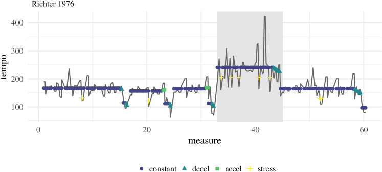
Figure 1: Note-by-note tempos for a recording of Chopin’s Mazurka Op. 68 No. 3 by Sviatislav Richter. The solid line are the observed tempos, while the dots represent inferred tempo states from our model.

Figure 1 shows the tempo in beats-per-minute (b.p.m.) of a recording made by Sviatislav Richter of Chopin’s Mazurka Op. 68 No. 3. The solid line shows the actual tempo at which he plays each note, while the colored points correspond to our model’s inferences for his actual intentions. Some of this intent is prescribed by Chopin in his music, but the extent to which Richter observes Chopin’s indications makes his recording different from those of other pianists. It is these differences that we hope to capture and understand.

1.1 Related work

The vast majority of work at the intersection of statistics or machine learning and classical music analysis has focused on a handful of tasks, most notably structure analysis, music generation, and score alignment.

Analysis of musical structure and its relationships with interpretation forms the basis of music theory, and hence constitutes the core of standard conservatory curricula, along with history and performance. Automatically learning musical structures from performances without expert input has become more relevant recently. Ren et al. (2010) use Dirichlet process models to identify similar sections of individual classical music performances. Roberts et al. (2018a) use variational autoencoders to learn long-term structure with an explicit goal toward improved automatic music composition.

Computer music generation and composition has a long history (Sturm et al., 2019; Boulanger-Lewandowski et al., 2012; Collins, 2016; Ariza, 2005; Flossmann et al., 2013). It is actively investigated, especially using deep learning (Hadjeres et al., 2017), and has become commercially relevant for advertising and video games through companies like Aiva (aiva.ai), and Melodrive (melodrive.com). Google has developed the Magenta project to enable open-source music composition (Roberts et al., 2018b).

The score alignment problem matches live or recorded performances to the musical score, a necessary processing step for any type of automated analysis. On-line alignment processes audio waveforms in real-time and is sometimes called score following (Dannenberg and Raphael, 2006; Cont, 2010; Cont et al., 2007; Arzt and Widmer, 2015). Audio matched to the score can then be used as an input for automated musical accompaniment (Raphael, 2010; Vercoe, 1984; Dannenberg, 1985). Given recorded accompaniment, these systems seek to modulate playback in response to a live soloist who both makes interpretive timing decisions and mistakes. Off-line alignment (Earis, 2007) can be used for simply analyzing the recordings, as we do here, or for generating features that describe the performance (Thickstun et al., 2017), possibly for later analysis in recommender systems (McFee and Lanckriet, 2011; van den Oord et al., 2013). For an overview of these and related goals in music information retrieval, see Schedl et al. (2014).

1.2 Our contributions

In this paper, we develop a switching Kalman filter model for the tempo decisions a performer makes in recorded classical music. We present an algorithm for performing likelihood inference, estimate our model using a large collection of recordings of the same composition, and demonstrate how the model is able to recover performer intentions, and how they relate to standard musical analysis. We use the learned low-dimensional representations to compare and contrast the recordings of different recordings through hierarchical clustering, and discuss how this analysis facilitates more informed musical comparisons of the recordings.

In Section 2 we discuss our dataset, a collection of professional recordings of Chopin’s Mazurka Op. 68 No. 3. We also present our model for tempo decisions, discuss it’s statistical estimation, and detail its utility for understanding interpretations as a musician would. Section 3 presents a music theory interpretation of the Mazurka. We discuss how different performers approach this piece through the lens of our model. We also examine a clustering based on our model and interpret the musical meaning of these clusters. Finally, we contrast our approach with some alternative non-parametric smoothers, discusses their deficiencies relative our switching model, and examine some issues with our proposal.

2 Materials and methods

In this paper, we examine note-by-note tempos for 46 recordings of Chopin’s Mazurka Op. 68, No.3. The data are part of a large collection of the complete Chopin Mazurkas and other recordings collected and analyzed by the Center for the History and Analysis of Recorded Music (CHARM) in the United Kingdom (CHARM, 2009). The recordings were processed using the note-onset detection algorithm developed in (Earis, 2007) and are available for download (Earis, 2009). We use the data for “all rhythmic events”, which includes the time of each note attack as well as it’s relative loudness.

2.1 Switching state-space models

State-space models define the probability distribution of a continuous time series $Y$ by reference to some imagined, continuous hidden state, $X$. In particular, the observation at time $i$ is assumed to be independent of past and future observations conditional on the state at time $i$. Coupling with temporal dependence for $X$—most frequently obeying the Markov property—induces a temporal model for the observations. The most general form of a state-space model is then characterized by the measurement equation (the conditional probability of observations given the states), the transition equation (specifying the nature of Markovian dynamics), and an initial distribution for the state:

$$y_{i} =f_{\theta}(x_{i},\epsilon_{i}), x_{i+1} =g_{\theta}(x_{i},\eta_{i}), x_{1} \sim F,$$ (1)

where $\epsilon_{i}$ are $\eta_{i}$ are marginally independent and identically distributed as well as mutually independent. Both $y_{i}$ and $x_{i}$ can be vector-valued, though in our application, $y_{i}$ will be univariate. The vector $\{y_{i}\}_{i=1}^{n}$ is observed, and the goal is to make inferences for the unobserved states $\{x_{i}\}_{i=1}^{n}$ as well as any unknown parameters $\theta$ characterizing $f_{\theta}$, $g_{\theta}$, and the distributions of $\epsilon_{i}$ and $\eta_{i}$.

If $f_{\theta}$ and $g_{\theta}$ are linear with $\epsilon_{i}$ and $\eta_{i}$ normally distributed, Equation (1) becomes

$$x_{i+1} =d+Tx_{i}+\eta_{i}, \eta_{i} \sim N(0,\ Q), x_{1} \sim N(x_{0},\ P_{0}),$$ (2)

$$y_{i} =c+Zx_{i}+\epsilon_{i}, \epsilon_{i} \sim N(0,\ G),$$

where the matrices $d,\ T,\ c,\ Z,\ Q,$ and $G$ are allowed to depend on $\theta$ and can potentially vary (deterministically) with $i$. In this case, the Kalman filter, (see e.g., Kalman, 1960; Harvey, 1990), provides closed form solutions for the conditional distributions of the states and gives the likelihood of $\theta$ given data. For completeness, we have included the Kalman filter in the Supplementary Material.

While the Kalman filter returns the likelihood for $\theta$, inference for the the mean and variance of $X$ is conditional only on the preceding observations $\{y_{j}\}_{j=1}^{i}$: ${\mathchoice{\raisebox{0.0pt}{$\displaystyle\upchi$}}{\raisebox{0.0pt}{$\textstyle\upchi$}}{\raisebox{0.0pt}{$\scriptstyle\upchi$}}{\raisebox{0.0pt}{$\scriptscriptstyle\upchi$}}}_{i}=\mathbb{E}\left[x_{i}\ |\ y_{1}\ldots,y_{i}\right]$ and $P_{i}=\mathbb{V}\left[x_{i}\ |\ y_{1},\ldots,y_{i}\right]$. To incorporate all future observations into these estimates, the Kalman smoother is required. There are many different smoother algorithms tailored for different applications. The smoother we use, due to Rauch et al. (1965), is often referred to as the classical fixed-interval smoother (Anderson and Moore, 1979). It produces only the unconditional expectations of the hidden state $\widehat{x}_{i}=\mathbb{E}\left[x_{i}\ |\ y_{1},\ldots,y_{n}\right]$ for the sake of computational speed. This version is more appropriate for inference in the type of switching models we discuss below. We again provide this algorithm in the Supplementary Material.

Linear Gaussian state-space models can be made quite flexible by expanding the state vector or allowing the parameter matrices to vary with time. Furthermore, this general form encompasses many standard time series models: ARIMA models, ARCH and GARCH models, stochastic volatility models, exponential smoothers, and more (see Durbin and Koopman, 2001, for many other examples). Nonlinear, non-Gaussian versions have been extensively studied (Durbin and Koopman, 1997; Fuh, 2006; Kitagawa, 1987, 1996) and algorithms for filtering, smoothing, and parameter estimation have been derived (e.g., Koyama et al., 2010; Andrieu et al., 2010). However, these models are less useful for change-point detection or other forms of discontinuous behavior when the times of discontinuity are unknown.

To remedy this deficiency, one can use a switching state-space model as shown in Figure 2. Here, we assume $S$ is a hidden, discrete process with Markovian dynamics. Then, the value of the hidden state at time $i$, $s_{i}=k$ say, can determine the evolution of the continuous model at time $i$. The graphical model in Figure 2 gives the conditional independence properties we will use in our model for musical interpretation, but this represents just one of many possibilities. Switching state-space models have a long history with many applications from economics (Kim and Nelson, 1998; Kim, 1994; Hamilton, 2011) to speech processing (Fox et al., 2011) to animal movement (Patterson et al., 2008; Block et al., 2011). An excellent overview of the history, typography, and algorithmic developments can be found in (Ghahramani and Hinton, 2000). In Equation (2), the parameter matrices were not time varying. In our switching model, we allow the switch states $s_{i},s_{i-1}$, along with the parameter vector $\theta$, to determine the specific dynamics at time $i$:

$$x_{1} \sim N(x_{0},\ P_{0}),$$ (3)

$$x_{i+1} =d(s_{i},s_{i-1})+T(s_{i},s_{i-1})x_{i}+\eta_{i}, \eta_{i} \sim N(0,Q(s_{i},s_{i-1})),$$

$$y_{i} =c(s_{i})+Z(s_{i})x_{i}+\epsilon_{i}, \epsilon_{i} \sim N(0,G(s_{i})).$$

In other words, the hidden Markov (switch) state determines which parameter matrices govern the evolution of the system.

Figure 2: Switching state space model. Filled objects are observed, rectangles are discrete, and circles are continuous.

2.2 A model for tempo decisions

In musical scores, tempi (the Italian plural of tempo) may be marked at various points throughout a piece of music. The beginning can be either explicit, with a metronome marking to indicate the number of beats per minute (b.p.m.), and/or with some words (e.g., Adagio, Presto, Langsam, Sprightly) which indicate an approximate speed.

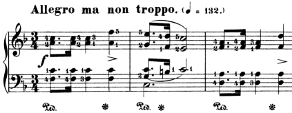
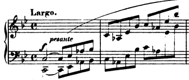
Figure 3: The beginning of two Chopin piano compositions: the Mazurka we analyze is on the left while the Ballade No. 1, Op. 23 is on the right.

Figure 3 shows the beginning of two Chopin piano compositions: the Mazurka we analyze and the Ballade No. 1, Op. 23. The initial tempo of the Mazurka is given with a metronome marking as well as the Italian phrase Allegro ma non troppo (“cheerful, but not too much”). The beginning of the Ballade is marked Largo, which translates literally as “broad” or “wide”, and modified by the stylistic indication pesante (“heavy”). Obviously, the metronome markings are much more exact, though even these are often viewed as suggestions rather than commandments. The metronome markings in most of Beethoven’s compositions, for example, are notoriously fast, and some scholars believe that his metronome (one of the first ever made) was inaccurate (Forsén et al., 2013). Often, compositions will have numerous such markings later in the piece of music, but these are only some of the ways that tempo is indicated. Composers will also indicate periods of speeding-up (accelerando) or slowing-down (ritardando).

Absent instructions from the composer, performers generally maintain (or try to maintain) a steady tempo, and this assumption plays a major role in our model of tempo decisions. Of course, a normal human never plays precisely like a metronome, although she may try quite hard to do so. The observed ratio of musical time to clock time is therefore best viewed as stochastic, the sum of an intentional, constant tempo, plus noise representing inaccuracy or, perhaps more charitably, unintentional variation which the listener fails to perceive as “wrong”. For instance, the example in Figure 4 shows the beginning of the piece as performed by Arthur Rubinstein in a 1961 recording.

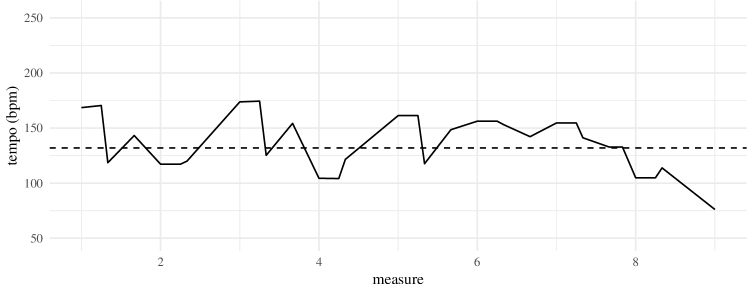
Figure 4: The solid line shows the observed note-by-note tempo for the beginning of the Mazurka as performed by Arthur Rubinstein in 1961. The dashed line indicates 132 b.p.m.

The solid line shows the actual, performed tempo, while the dashed horizontal line is placed at the indicated tempo of 132 b.p.m. The figure has three important lessons: (1) observed speed varies around intended tempo; (2) 132 b.p.m. is not necessarily the tempo a performer will choose despite the indication; and (3) performers have other tempo intentions which are not marked, like the pronounced slow-down in measures 7–8.

Estimating intended tempi would be reasonably simple, perhaps, if the locations of the tempo changes were known. In such a case, the average of tempi between changes may be a good estimate as could the slope of known speed-ups or slow-downs. However, performers take liberties with these decisions, exactly the liberties we would like to discover. This suggests employing a switching model with a small number of discrete states.

Similar to Gu and Raphael (2012), we propose a Markov model for $S$ on four states for four different performance behaviors with transition probability diagram given by Figure 5.

Figure 5: Transition diagram. The four states are: constant tempo (1), deceleration (2), acceleration (3), and emphasis (4).

The 4 switch states correspond to 4 different behaviors for the performer: (1) constant tempo, (2) speeding up, (3) slowing down, and (4) single note stress. As shown in the diagram, we only allow certain transitions for musical reasons and for estimability. The marked transition probabilities are sufficient to infer the remainder. The fourth state, stress, corresponds to tenuto, a common feature of musical performance. Such stresses may be marked with a line over the note in question, but are more often a feature of the performer taste, corresponding to a longer-than-written duration of a particular note. Such emphases occur for a variety of musical purposes—emphasis of the beat in running notes, the top of a phrase, a “landing point” where a phrase ends, etc.—but are always within the frame of constant tempo. Thus we allow stress to occur only after and before notes in state 1. Furthermore, we cannot allow state 2 or state 3 to return immediately to state 1, or else “stress” could happen through these pathways. We impose related constraints for a transition from state 2 to state 3 and vice versa. Essentially, transitions into these states must remain there before leaving. Thus, the entire transition diagram is fully determined. This process can be viewed equivalently as a second-order Markov chain.

Our data gives $y_{i}$ as the observed tempo (in b.p.m.) of the note (or chord) of the $i^{th}$ note onset in Chopin’s Mazurka Op. 68 No. 3. The hidden continuous variable ($X_{i}$) is taken to be a two component vector with the first component being the prevailing tempo and the second the amount of acceleration. The amount, or existence, of acceleration is determined by the current and previous switch states. We use $l_{i}$ to denote the musical duration of a particular note as given by the written score, so, throughout this piece, a quarter-note (𝅘𝅥) has $l_{i}=1/3$, an eighth note (𝅘𝅥𝅮) has $l_{i}=1/6$, etc. This is because each measure contains three quarter notes. In more complicated music with changing time signatures or instances where the notation doesn’t necessarily correspond with the time signature, more care would be required. The observed tempo is already normalized to account for variable note durations, but the intentional tempo and its variance should be proportional to $l_{i}$. When the performer is in state 1 (or transits in and out of state 4), we take the prevailing tempo as constant with no acceleration: $X_{i+1}=X_{i}$. Corresponding to these configurations, the parameter matrices are given in Table 1 (transition equation) and Table 2 (measurement equation).

Switch states			parameter matrices
$s_{i}$	$s_{i-1}$		$d$	$T$	$Q$
$1$	$1$		0	$\begin{pmatrix}1&0\\ 0&0\end{pmatrix}$	$\begin{pmatrix}0&0\\ 0&0\end{pmatrix}$
$2$	$1$		$\begin{pmatrix}l_{i}\mu_{\textrm{acc}}\\ \mu_{\textrm{acc}}\end{pmatrix}$	$\begin{pmatrix}1&0\\ 0&0\end{pmatrix}$	$\sigma_{\textrm{acc}}^{2}\begin{pmatrix}l_{i}^{2}&l_{i}\\ l_{i}&1\end{pmatrix}$
$3$	$1$		$\begin{pmatrix}-l_{i}\mu_{\textrm{acc}}\\ -\mu_{\textrm{acc}}\end{pmatrix}$	$\begin{pmatrix}1&0\\ 0&0\end{pmatrix}$	$\sigma_{\textrm{acc}}^{2}\begin{pmatrix}l_{i}^{2}&l_{i}\\ l_{i}&1\end{pmatrix}$
$4$	$1$		$\begin{pmatrix}0\\ \mu_{\textrm{stress}}\end{pmatrix}$	$\begin{pmatrix}1&0\\ 0&0\end{pmatrix}$	$\begin{pmatrix}0&0\\ 0&\sigma_{\textrm{stress}}^{2}\end{pmatrix}$
$2$	$2$		0	$\begin{pmatrix}1&l_{i}\\ 0&1\end{pmatrix}$	$\begin{pmatrix}0&0\\ 0&0\end{pmatrix}$
$3$	$2$		$\begin{pmatrix}-l_{i}\mu_{\textrm{acc}}\\ -\mu_{\textrm{acc}}\end{pmatrix}$	$\begin{pmatrix}1&0\\ 0&0\end{pmatrix}$	$\sigma_{\textrm{acc}}^{2}\begin{pmatrix}l_{i}^{2}&l_{i}\\ l_{i}&1\end{pmatrix}$
$1$	$2$		$\begin{pmatrix}\mu_{\textrm{tempo}}\\ 0\end{pmatrix}$	0	$\begin{pmatrix}\sigma^{2}_{\textrm{tempo}}&0\\ 0&0\end{pmatrix}$
$3$	$3$		0	$\begin{pmatrix}1&l_{i}\\ 0&1\end{pmatrix}$	$\begin{pmatrix}0&0\\ 0&0\end{pmatrix}$
$2$	$3$		$\begin{pmatrix}l_{i}\mu_{\textrm{acc}}\\ \mu_{\textrm{acc}}\end{pmatrix}$	$\begin{pmatrix}1&0\\ 0&0\end{pmatrix}$	$\sigma_{\textrm{acc}}^{2}\begin{pmatrix}l_{i}^{2}&l_{i}\\ l_{i}&1\end{pmatrix}$
$1$	$3$		$\begin{pmatrix}\mu_{\textrm{tempo}}\\ 0\end{pmatrix}$	0	$\begin{pmatrix}\sigma^{2}_{\textrm{tempo}}&0\\ 0&0\end{pmatrix}$
$1$	$4$		0	$\begin{pmatrix}1&0\\ 0&0\end{pmatrix}$	$\begin{pmatrix}0&0\\ 0&0\end{pmatrix}$

Table 1: Parameter matrices of the transition equation for the switching state space model.

Switch states			parameter matrices
$s_{i}$			$c$	$Z$	$G$
$4$			0	$\begin{pmatrix}1&1\end{pmatrix}$	$\sigma^{2}_{\epsilon}$
else			0	$\begin{pmatrix}1&0\end{pmatrix}$	$\sigma^{2}_{\epsilon}$

Table 2: Parameter matrices of the measurement equation for the switching state space model.

So for any performance, we want to be able to estimate the following parameters: $\sigma_{\textrm{tempo}}^{2}$, $\sigma_{\textrm{acc}}^{2}$, $\sigma^{2}_{\textrm{stress}}$, $\sigma_{\epsilon}^{2}$, the probabilities of the transition matrix (there are 7), and means $\mu_{\textrm{tempo}}$, $\mu_{\textrm{acc}}$, and $\mu_{\textrm{stress}}$. Lastly, we have the initial state distribution

$$x_{1}\sim N\left(\begin{pmatrix}\mu_{1}\\ 0\end{pmatrix},\ \begin{pmatrix}\sigma^{2}_{1}&0\\ 0&0\end{pmatrix}\right)\;\;\textrm{where}\;\;s_{1}=1.$$

To clarify this model, we explicate two different behaviors: discrete sequence $1\rightarrow 4\rightarrow 1$ (emphasis within constant tempo) and discrete sequence $1\rightarrow 1\rightarrow 2$ (constant tempo to slowing down). In the first case, the state space system has the following configurations

$$1\rightarrow 4 4\rightarrow 1$$

$$x_{2} =\begin{pmatrix}0\\ \mu_{\textrm{stress}}\end{pmatrix}+\begin{pmatrix}1&0\\ 0&0\end{pmatrix}x_{1}+\mbox{N}\left(0,\ \begin{pmatrix}0&0\\ 0&\sigma_{\textrm{stress}}^{2}\end{pmatrix}\right) x_{3} =\begin{pmatrix}1&0\\ 0&0\end{pmatrix}x_{2}$$

$$y_{2} =(1\quad 1)x_{2}+\mbox{N}(0,\ \sigma_{\epsilon}^{2}) y_{3} =(1\quad 0)x_{3}+\mbox{N}(0,\ \sigma_{\epsilon}^{2}),$$

while in the second

$$1\rightarrow 1 1\rightarrow 2$$

$$x_{2} =\begin{pmatrix}1&0\\ 0&0\end{pmatrix}x_{1} x_{3} =\begin{pmatrix}l_{i}\mu_{\textrm{acc}}\\ \mu_{\textrm{acc}}\end{pmatrix}+\begin{pmatrix}1&0\\ 0&0\end{pmatrix}x_{1}+\mbox{N}\left(0,\ \sigma_{\textrm{acc}}^{2}\begin{pmatrix}l_{i}^{2}&l_{i}\\ l_{i}&1\end{pmatrix}\right)$$

$$y_{2} =(1\quad 0)x_{2}+\mbox{N}(0,\ \sigma_{\epsilon}^{2}) y_{3} =(1\quad 0)x_{3}+\mbox{N}(0,\ \sigma_{\epsilon}^{2}).$$

Recall that in any case $y_{i}$ is a scalar and $x_{i}\in\mathbb{R}^{2}$.

2.3 Estimation and computational issues

To understand the performance decisions of individual musicians, we wish to simultaneously learn $\theta$, $S$, and $X$. Because the switch states $S$ and the continuous states $X$ are both hidden, this becomes an NP-hard problem. In particular, there are $4^{n}$ possible paths through the switch variables, so evaluating the likelihood to maximize over $\theta$ via the Kalman filter at each path is intractable. Ghahramani and Hinton (2000) give a variational approximation to estimate $\theta$ without also estimating $S$, but, as our goal is to learn both, we use the particle filtering approximation described by Fearnhead and Clifford (2003).  Whiteley et al. (2010) refer to this algorithm as the Discrete Particle Filter, and it can be seen as an instance of the “Beam Search” optimization technique (Bisiani, 1992). The details are given in Algorithm 1 but the intuition is as follows: (1) for the first few time points, evaluate one step of the Kalman filter for each possible subsequent discrete state and store all these values; (2) calculate weights for each path by updating previous weights with the likelihood multiplied by the transition probability; (3) continue through time until the number of stored values exceeds some threshold storage limit; (4) from that point forward, subselect the “best” paths using a sampling scheme.

Algorithm 1 Discrete particle filter

1:  Input: $Y$, $\theta$, $\pi_{1}$ probability vector over initial states (paths), $B$ maximum beam width

2:  for $i=1$ to $n$ do

3:     Set $b_{i}=|\{\pi_{i}>0\}|$, the number of current paths

4:     Use the Kalman filter to calculate the 1-step likelihood $\ell_{i}$ for each path and every potential state $s_{i+1}$ resulting in $b_{i}|S|$ particles

5:     Set $\pi_{i+1}\leftarrow\pi_{i}\ell_{i}p_{i}$: multiply the path probability by the likelihood and the probability of transitioning. Normalize $\pi$.

6:     Set $b_{i+1}=|\{\pi_{i+1}>0\}|$ . If $b_{i+1}>B$, resample the weights to get $B$ non-zero weights and renormalize

7:  end for

8:  Return $B$ paths $\{S_{b}\}_{b=1}^{B}$ along with their weights $\pi_{n}$.

These paths can be selected greedily, retaining only the highest values to that point, though we use the resampling procedure of (Fearnhead and Clifford, 2003) which is designed to approximate to the full discrete distribution over paths with a subset of support points by minimizing the mean squared error.

Algorithm 1 returns $B$ paths along with their weights through the discrete state $S$ for a particular parameter value $\theta$. One can view this as a (approximate) distribution over paths conditional on $\theta$. Instead, we will simply take the path with the highest weight for inference via penalized maximum likelihood. Thus, the likelihood of a particular parameter vector $\theta$ is evaluated by computing the best path with Algorithm 1 and then using the best path with the Kalman filter.

2.4 Penalized maximum likelihood

Even without the latent discrete states, parameter estimation in state-space models is a difficult problem, often plagued by spurious local minima and non-identifiability. The addition of discrete states only exacerbates this issue. However, for the present application, we have reasonably strong prior information for many of the parameters. The three mean parameters $\mu_{\textrm{tempo}}$, $\mu_{\textrm{acc}}$ and $\mu_{\textrm{stress}}$ have sign restrictions in addition to strong information about their magnitude: average tempo should be around the indicated 132 b.p.m., the average amount of acceleration should probably be less than the size of a stress. We also have reasonably strong information about the probabilities of transitioning between states: self-transitions should be reasonably likely, long periods of speeding up are less likely than long periods of slowing down which are less likely than long periods in the constant tempo state. Because of this information, we use informative priors as penalties on all the parameters we estimate. This has the effect of introducing extra curvature to the optimization problem as well as conforming with musical intuition. The specific choices are shown in Table 3.

Parameter		Distribution	Prior mean
$\sigma^{2}_{\epsilon}$	$\sim$	Gamma$(40,\ 10)$	400 b.p.m.2
$\mu_{\textrm{tempo}}$	$\sim$	Gamma$(\overline{Y}^{2}/100,\ 100/\overline{Y})$	$\overline{Y}$ b.p.m.
$-\mu_{\textrm{acc}}$	$\sim$	Gamma$(15,\ 2/3)$	10 b.p.m.
$-\mu_{\textrm{stress}}$	$\sim$	Gamma$(20,\ 2)$	40 b.p.m.
$\sigma^{2}_{\textrm{tempo}}$	$\sim$	Gamma$(40,\ 10)$	400 b.p.m.2
$\sigma^{2}_{\textrm{acc}}$	$=$	1	1 b.p.m.2
$\sigma^{2}_{\textrm{stress}}$	$=$	1	1 b.p.m.2
$p_{1,\cdot}$	$\sim$	Dirichlet$(85,\ 5,\ 2,\ 8)$
$p_{2,\cdot}$	$\sim$	Dirichlet$(4,\ 10,\ 1,\ 0)$
$p_{3,\cdot}$	$\sim$	Dirichlet$(5,\ 3,\ 7,\ 0)$

Table 3: Informative prior distributions for the music model

We fix $\sigma^{2}_{\textrm{acc}}$ and $\sigma^{2}_{\textrm{stress}}$ after numerical experiments suggested that they were poorly identified.

2.5 Is this model reasonable?

It is reasonable to ask whether a simple model such as this is able to accurately represent performance practice without removing musically important information. In a statistical sense, this question is similar to the problem of tuning parameter selection in nonparametric estimation. Specifically, we do not want this model to “over-smooth” the performance, eliminating information necessary for listener appreciation. One way to examine such a question is to generate a performance using the smoothed tempos learned by the model and compare it aurally with the original recording. Gu and Raphael (2012) used a model similar to ours to investigate just this question. In one study, they surveyed nine graduate piano majors at a major conservatory on twelve different piano excerpts. The pianists were not meaningfully able to distinguish between the synthesized and real recordings in the majority of experiments. Our model is more expressive than that employed in the study, and the parameters are estimated from data rather than calibrated. We expect that a similar study with our model would yield similar, if not better, results.

3 Analysis of Chopin’s Mazurka Op. 68 No. 3

We use the model and procedures developed above to estimate the parameters and performance choices for all 46 recordings of Chopin’s Mazurka. Here we describe the inferences our model allows on some representative performances, describe parametric clusters determined by our model, contrast these with some alternative approaches to music modelling, and discuss some difficulties we encountered. All simulations and empirical calculations were performed with R (R Core Team, 2019) and C++ via Rcpp (Eddelbuettel, 2013). Figures and tables are generated using the tidyverse family of packages (Wickham, 2017, 2016). Dendrograms combined with heatmaps for the proximity matrices were created with the heatmaply package (Galili et al., 2017). Most computations were implemented in parallel on a large memory computer cluster via the batchtools package (Lang et al., 2017).

3.1 Musical analysis

Throughout his life, Frédéric Chopin composed dozens of Mazurkas, of which 58 have been published. Inspired by a traditional Polish dance, these pieces gave Chopin an idiomatic style upon which to elaborate a wide variety of different compositional techniques, a practice German and Italian composers had employed frequently over the previous 3 centuries (Burkholder et al., 2014). Repetition of themes, figures, or even small motives plays a central role in both the traditional dance and Chopin’s compositions as do particular rhythmic gestures (Kallberg, 1996), especially the dotted-eighth sixteenth note pattern on the first beat of a measure.

Chopin’s Op. 68 Mazurkas are a set of four similar works, published posthumously in 1855. The Op. 68 No. 3, which we analyze here, was composed in 1830, when Chopin was 20 years old. Around this time, Chopin, already a piano virtuoso and accomplished composer, left his native Warsaw and settled in Paris, where we would remain until his death in 1849.

This Mazurka has a rather simplistic ternary structure with two outer sections and a contrasting middle (ABA). The first A section is made up of four eight-bar phrases ($aaba$). The first phrase is echoed by the second phrase: they are nearly identical, with the two exceptions being that (1) the second is marked piano (soft) rather forte (strong) and (2) the second ends on the tonic (F major) rather than the dominant (C major). The fourth eight-bar phrase is an exact repetition of the second. The second A section is a repeat of the first two eight-bar phrases of the beginning. The intervening B section is 12 bars long, divided into three four-bar groups. The first four bars are simply a repeated interval of a perfect $5^{th}$ in the left hand. This ostinato will continue for the whole section. The remaining eight measures consist of a four-bar phrase in the right hand repeated twice. The second differs from the first only on the final two notes, preparing the recapitulation of the A section.

In terms of tempi, the B section is indicated to be faster, with the marking Poco più vivo (a little livelier). The B section ends with a ritardando into the following A section. The $b$ section ends with a fermata in measure 24, indicating an arbitrary elongation while the piece concludes with a two-measure long ritardando. Throughout, frequent markings prescribe emphasis of the third beat of each measure. This emphasis is in keeping with the mazurka style, an intentional thwarting of the listener’s expectation of first-beat emphasis.

Figure 6 shows the first ten measures of the musical score with annotations for the sections discussed above and the harmonic progression in Roman numerals below the staff.

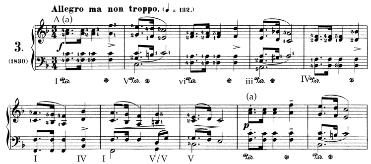
Figure 6: The first ten measures of Chopin’s Mazurka Op. 68, No. 3. The harmonic progression is indicated below the staff in Roman numerals. Sections are marked above the staff, e.g., A (a). Analysis by the authors. This image comes from the complete score published by Bote and Bock in 1880. This composition is in the public domain, and the score is freely available via the International Music Score Library Project.

The harmonies are standard, in fact, they are essentially the same as those of Pachelbel’s Canon, familiar to many as “that song played at weddings.” These harmonies, combined with the rhythmic repetition suggests a further division of this and all analogous sections into three small groupings: two two-measure phrases, followed by a four-measure phrase.

As a performer, these harmonic, rhythmic, and structural analyses aid in interpretation. The performer needs to decide how to emphasize or deemphasize these demarcations with slight or overt tempo or dynamic alterations. In a live performance, she could use physical motion to further suggest a particular interpretation. She can choose to emphasize long phrases, in this case, phrases of eight measures, or the shorter sub-phrases. Because of the repetition of similar phrases, she may choose to emphasize the long phrase on the first occurrence and shorter sub-phrases later on for variety, for example. While the musical structure suggests such possible interpretations, the performer must make these choices on their own, and may even alter those decisions from performance to performance.

3.2 Archetypal performances

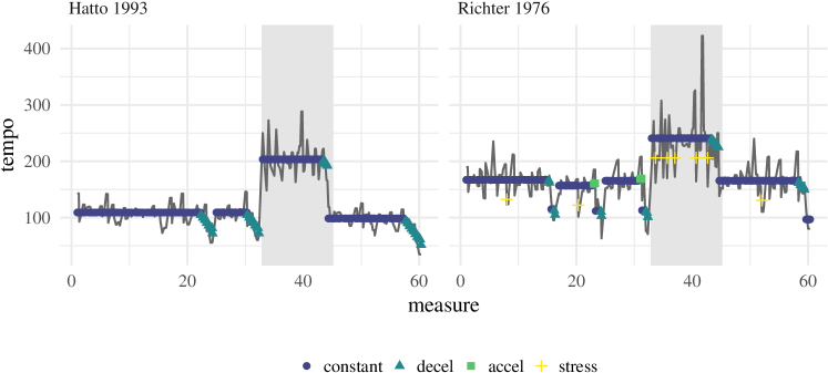
Figure 7: Inferred performer choices for two recordings.

Here we will carefully investigate how our model learns interpretive decisions for three rather different performances. Figure 7 shows the inferred state sequence for recordings made by Joyce Hatto in 1993 and Sviatislav Richter in 1976. The B section is shaded in gray to better illustrate the formal divisions discussed above.

In terms of our model, these two performers are quite different from each other. Hatto maintains a constant tempo carefully, remaining in state 1 with the exception of four periods of deceleration. All four periods coincide with the most significant phrase endings: at the end of the A section at measure 32, the end of the B section at measure 48, at the end of the piece, and the minor transition from $b\rightarrow a$ in the first A section (measure 24). According to our inferred model, she never accelerates or uses the transitory stress state.

In contrast, Richter uses all four states from our model. The short blips of acceleration before the B section and before the $b\rightarrow a$ transition are slightly out of place, and are likely better labelled as “constant”, but these state transitions describe more severe decelerations than the model’s linear assumption would allow. Richter uses stress frequently. Some may well be attributable to larger variance around constant tempo (picked up as frequent stress rather than larger $\sigma^{2}_{\epsilon}$), but most correspond to interesting note emphases, for example the second beat of measure 20. This note is essentially a minor phrase ending, but is also marked in the score with a sforzando (with sudden emphasis). It’s the first of two such occurrences in the piece, the second coming four measures later on the fermata, Richter’s slowest note in the entire piece. Richter likely chooses to make this prescribed emphasis with a sudden slow down in part because it takes place within the context of an already loud passage, precluding the use of extra volume.

Table 4: The estimated parameters for performances by Richter and Hatto.

	$\sigma^{2}_{\epsilon}$	$\mu_{\textrm{tempo}}$	$\mu_{\textrm{acc}}$	$\mu_{\textrm{stress}}$	$\sigma^{2}_{\textrm{tempo}}$	$p_{11}$	$p_{12}$	$p_{22}$	$p_{31}$	$p_{13}$	$p_{21}$	$p_{32}$
Richter 1976	426.70	136.33	-11.84	-34.82	439.38	0.85	0.05	0.74	0.44	0.02	0.25	0.17
Hatto 1993	405.57	130.36	-13.57	-27.93	408.99	0.94	0.03	0.82	0.36	0.01	0.16	0.19
Cortot 1951	403.71	182.84	-21.43	-45.67	460.82	0.92	0.02	0.71	0.34	0.03	0.23	0.09

Table 4 shows the estimated parameters for these two performances. Richter has larger observation variance, $\sigma^{2}_{\epsilon}$, slightly faster average tempo, lower acceleration, and larger stress. He also has a larger tempo variance, meaning that returns to state 1 can start at relatively different tempos. On the other hand, Hatto is much more likely to remain in states 1 or 2. These inferences are largely consistent with the visual takeaways of Figure 7. It’s easy to see the increased variability around the constant tempo in Richter’s performance and the faster overall tempos in both the A and B sections. While these two performances are quite different from each other, they also display similarities. Both take a faster tempo in the B section versus the A sections. Both performers slow down at the end of the piece, at the end of the B section, immediately preceding the B section, and at the $b\rightarrow a$ transition.

Alfred Cortot’s 1951 performance is displayed in Figure 8. Both in terms of the parametric model we propose, and if we simply compare the vectors of note-by-note tempos (discussed in more detail below), this performance is an outlier. Cortot never uses the deceleration state, and he remains in constant tempo for the entirety of both A sections. While the model describes his performance well, it also illustrates a deficiency of this approach: Cortot, more than any other performer, has large contrasts between the A and B sections. His A section is the slowest of all 46 recordings at around 64 b.p.m., half the marked tempo. The next slowest is Maryla Jonas’s recording at around 84 b.p.m. Meanwhile, his B section is among the fastest of all the recordings and contains the fastest individual note. Additionally, there is stunningly little tempo variability in his A sections, but dramatic variation in the B section coupled with frequent uses of the acceleration and emphasis states. Taken together, Cortot’s performance may be better described by estimating our model separately on the two sections.

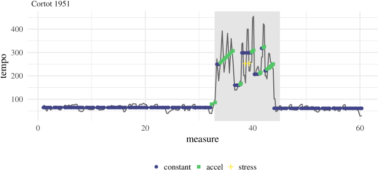
Figure 8: Inferred performance choices for Alfred Cortot’s 1951 recording.

3.3 Clustering musical performances

To better understand how all the 46 performances relate to each other, we applied parametric clustering using the eleven-dimensional vector of estimated parameters. Because the estimated parameters are of different scales, have different domains, and can covary, we treat them differentially. To calculate distances between the mean and variance parameters, $\sigma^{2}_{\epsilon}$, $\mu_{\textrm{tempo}}$, $\mu_{\textrm{acc}}$, $\mu_{\textrm{stress}}$, and $\sigma^{2}_{\textrm{tempo}}$ we simply use Euclidean distance on each individually. In the cases of the probabilities, we use weighted Euclidean distance in the prior precision. For example, for $p_{1\cdot}$, we calculate

$$d\left(p_{1\cdot},\ p^{\prime}_{1\cdot}\right)=(p_{1\cdot}-p^{\prime}_{1\cdot})^{\top}\Omega(p_{1\cdot}-p^{\prime}_{1\cdot}),\quad\textrm{where}\quad\Omega^{-1}_{ij}:=\Sigma_{ij}:=\alpha_{0}^{-2}(\alpha_{0}+1)^{-1}\left(\alpha_{i}\alpha_{0}\delta_{ij}-\alpha_{i}\alpha_{j}\right),$$ (4)

is the covariance matrix of the Dirichlet distribution with $\alpha_{0}=\sum_{i}\alpha_{i}$ and $\delta_{ij}$ the indicator that $i=j$. We then standardize each individual distance matrix to have a maximum distance of 1 and add them together so that the maximum distance between performances is 8.

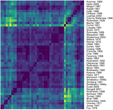
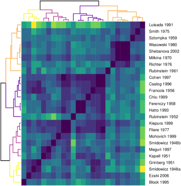
Figure 9: Distance matrix using estimated model parameters. Left: the matrix for all 46 parameters. Right: The same matrix with “outlying” performances removed and a dendrogram from hierarchical clustering.

Figure 9 shows the distance matrix calculated from the estimated parameters for all 46 performances (left) and the same matrix with “outlying” performances removed (right). To determine outlying performances, we calculated the distance to the third nearest performance. We then removed those performances that exceeded a threshold, meaning that the nearest similar performances were “far away”. This screening left 25 performances. We used hierarchical clustering on these 25 performances, trying between two and five clusters. The remaining 21 were grouped together as “other”. The right panel of Figure 9 displays this subset along with a dendrogram and four clusters.

Figure 10: Cluster densities for Markov transition probabilities.

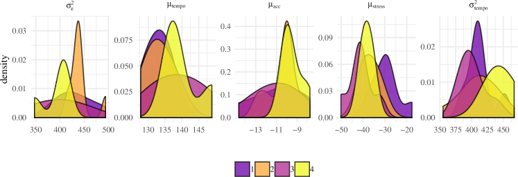
Figure 11: Cluster densities for mean and variance parameters.

The first cluster corresponds to performances which are reasonably staid. The emphasis state is rarely visited with the performer tending to stay in the constant tempo state with periods of slowing down at the ends of phrases. Acceleration is never used. Such state preferences are clearly inferred by the model as shown in the top row of Figure 10. Furthermore, these performances have relatively low average tempos, and not much difference between the A and B sections. Joyce Hatto’s performance shown in Figure 7 is typical of this cluster.

Recordings in the second cluster tend to transition quickly between states, especially constant tempo and slowing down accompanied by frequent transitory emphases. The probability of remaining in state 1 is the lowest while the probability of entering state 2 from state 1 is the highest. The acceleration state is rarely visited. Four of the most similar performances are in this cluster, shown in Figure 12, along with Richter’s 1976 recording.

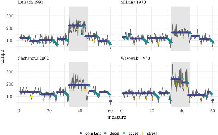
Figure 12: Four similar performances, all in the second cluster.

Cluster three is somewhat like cluster one in that performers tend to stay in state 1 for long periods of time, but they transition more quickly from state 3 back to state 1. They also use state 4 frequently whereas cluster one did not. They tend to have very large tempo contrasts between the A and B sections. Cluster four has both faster average tempos and more variability from one period of constant tempo to the next. State 4 is rare, instead using constant tempo states that persist for small amounts of time to reflect note emphases.

Comparing our clusters to those we would find from simply clustering the distances between note-by-note tempo vectors reveals a number of differences (see the Supplement for the distance matrix calculated in this way). The four recordings in Figure 12 would be spread across three different clusters, for example, as would our cluster one. On the other hand, both metrics see Cortot’s recording as a strong outlier, and clustering by tempo vectors often (somewhat miraculously) groups recordings by the same pianist together: both recordings by Smidowicz, three of the four recordings by Rubinstein, both recordings by Hatto.

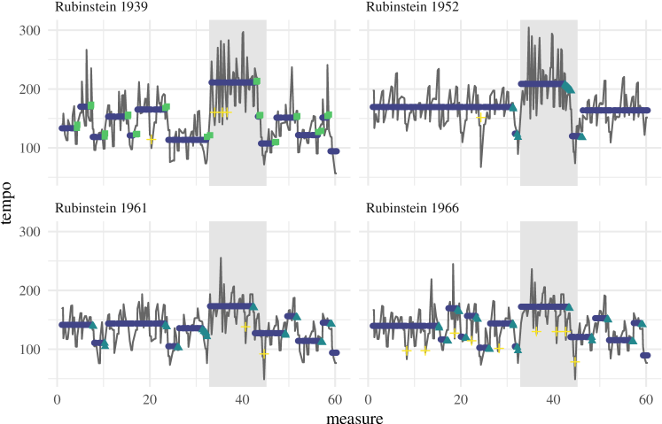
Figure 13: The four recordings by Arthur Rubinstein. Our clustering puts the 1952 and 1961 recordings in clusters one and two while leaving the others out. Clustering by tempo vector separates 1952 from the other three.

Figure 13 shows all four Rubinstein recordings. The 1939 recording is rather odd in that the measures 24–32 are so slow relative to the rest of the A section. The variability in the 1966 recording nearly obscures the contrast between the B section and the surrounding A sections. These two recordings are nonetheless clustered together by the tempo vectors. Our method on the other hand, puts both in the “other” grouping. The estimated parameters for these four performances are shown in the bottom half of Table 5. The top half shows the parameters for the four similar performances in Figure 12. There is much larger variability across Rubinstein’s recordings, as we would expect.

Table 5: The estimated parameters for the four similar performances in Cluster Two and those for all four by Arthur Rubinstein.

	$\sigma^{2}_{\epsilon}$	$\mu_{\textrm{tempo}}$	$\mu_{\textrm{acc}}$	$\mu_{\textrm{stress}}$	$\sigma^{2}_{\textrm{tempo}}$	$p_{11}$	$p_{12}$	$p_{22}$	$p_{31}$	$p_{13}$	$p_{21}$	$p_{32}$
Wasowski 1980	414.99	132.00	-10.00	-40.00	425.00	0.85	0.05	0.67	0.34	0.02	0.26	0.20
Shebanova 2002	439.98	132.00	-10.00	-40.00	400.02	0.85	0.05	0.67	0.33	0.02	0.27	0.20
Luisada 1991	494.33	127.80	-10.24	-32.56	411.63	0.84	0.10	0.71	0.35	0.01	0.26	0.19
Milkina 1970	435.25	136.38	-9.68	-40.02	400.01	0.87	0.05	0.68	0.33	0.02	0.26	0.21
Rubinstein 1939	520.32	145.26	-7.89	-50.82	345.64	0.89	0.02	0.83	0.56	0.05	0.13	0.16
Rubinstein 1952	481.13	128.13	-7.76	-17.59	409.30	0.93	0.04	0.68	0.32	0.01	0.28	0.19
Rubinstein 1961	434.23	139.17	-8.34	-35.08	355.00	0.90	0.06	0.56	0.46	0.01	0.41	0.19
Rubinstein 1966	380.95	127.24	-8.80	-42.28	473.69	0.87	0.07	0.36	0.34	0.01	0.61	0.20

3.4 Alternative smoothers

Our model is just one type of smoothing one could imagine using to find low-dimensional structure for the vector of note-by-note tempos. Alternative statistical techniques are common, and examining how they compare with our method helps to illuminate some of its benefits. The most obvious alternative is to use smoothing splines (Craven and Wahba, 1978; Wahba, 1990) though total-variation denoising or trend filtering (Kim et al., 2009; Tibshirani, 2014) are other reasonable alternatives. These statistical techniques perform smoothing by encouraging small changes in derivatives (smoothing splines) or bounded total variation (trend filtering). But musical performances do not conform to these assumptions because tempo interpretations rely on the juxtaposition of local smoothness with sudden changes and emphases to create listener interest. It is exactly the parts of a performance that are poorly described by statistical smoothers that render a performance interesting. Furthermore, many of these inflections are notated by the composer or are implicit in performance practice developed over centuries of musical expressivity. Consequently, smoothing that incorporates domain knowledge leads to better statistical and empirical results.

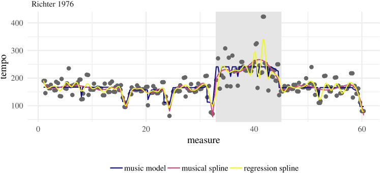
Figure 14: Smoothing with splines and musical models

Figure 14 shows the note-by-note tempo of Richter’s 1976 recording. Splines with equally spaced knots are shown in yellow. We use generalized cross validation (Golub et al., 1979) to select the number of knots (one knot per measure). The red line shows a regression spline fewer knots, but whose locations were chosen manually to coincide with the musical phrase endings discussed in Section 3.1. Knots at phrase endings were duplicated up to four times to allow for discontinuities. The blue line shows the estimated smooth tempo from our model (the same as in Figure 7). The regression spline with equally spaced knots undersmooths in constant tempo areas in an attempt to capture sudden emphases and dramatic changes in others. The spline with informed knot choice does much better, picking up the periods of deceleration at the ends of phrases. Our model learns these behaviors on its own while also capturing individual emphases that are missed in the musical analysis but are idiosyncratic to Richter’s playing. It is also more parsimonious to musical interpretation, inferring constant tempo periods rather than resulting in smoothly varying tempos in stable periods.

3.5 Problems with the model and estimation

While our model of musical decision making yields interesting insights into performance practice most of the time, it also suffers from some deficiencies. As discussed above in reference to Alfred Cortot’s recording, the assumption that all parameters are stable over the entire piece may not always be accurate. The $\mu_{\textrm{tempo}}$ parameter especially, should be estimated separately in different sections. This problem will only be compounded in more complex music with many contrasting sections. A related issue is the current form for the slowing down and speeding up sections. Our model assumes that both occur linearly, with a constant decrease of $\mu_{\textrm{acc}}$ b.p.m. An ability to slow increasingly as one remains in the state may improve the model fit.

There is nothing intrinsic to the model which forces states 2, 3, or 4 to always go in the correct direction. If for example, $\mu_{\textrm{acc}}$ is small in magnitude relative to $\sigma^{2}_{\textrm{acc}}$, an acceleration could be learned as time spent in state 2 but with large positive errors. For this piece, the penalties help to avoid such occurrences, but this aspect of the Gaussian state-space model could be improved by enforcing non-Gaussian behavior. Or course, such constraints would complicate likelihood evaluation since the Kalman filter could no longer be used. Relatedly, our model produced objectively incorrect inferences on two performances

Figure 15: Estimation errors on two performances.

(Figure 15). Here, the estimated path failed to transition to state 1 at the recapitulation of the A section. In both cases, the resulting path stands out dramatically, remaining in the much faster constant tempo state from the B section with overly frequent emphases. Both of these performances are quite volatile, making estimation difficult, and were clustered as “other”.

4 Discussion

Musical interpretation is the most important factor in determining whether or not concertgoers enjoy a classical performance. Every performance includes mistakes—intonation issues, a lost note, an unpleasant sound—but these are all easily forgotten (or unnoticed) when a performer engages her audience, imbuing a piece with novel emotional content beyond the vague instructions inscribed on the printed page. While music teachers use imagery or heuristic guidelines to motivate interpretive decisions, combining these vague instructions to create a convincing performance remains the domain of the performer, subject to the whims of the moment, technical fluency, and taste.

In this paper, we develop a statistical model for tempo to elucidate performance decisions from classical music recordings. We present an algorithm for performing likelihood inference, estimate our model using a large collection of recordings of the same composition, and demonstrate how the model is able to recover performer intentions, and how they relate to standard musical analysis. While our methods perform well, our analysis reveals a number of avenues for future work an improvement. For the piano, apart from tempo decisions, the performer can also control dynamics differentially. Similar techniques to those employed here could be used to describe levels of loudness, and creating a model that combined both is desirable. Pianists have relatively few variables under their control for interpretation: tempo, dynamics, and pedalling. On the other had, string players have many more. Bowing decisions, fingerings, vibrato, broken chords are all important tools which are difficult to learn from a recording, let alone describe with a simple statistical model. Significant work would be required to generalize our techniques to more detailed interpretative analysis. On the other hand, focusing simply on tempo can be useful with solo performances or with larger ensembles. Examining more complex genres—sonatas, string quartets, symphonies—would also be interesting for future work.

Another avenue we wish to pursue in the future is to examine how our model’s implications may be useful for teaching students. Can we estimate it quickly to provide immediate feedback to novice pianists? In this paper, we used a dataset in which the note-by-note tempos were annotated by experienced musicians. Combining our model with existing approaches to solving the note-score alignment problem (Lang and Freitas, 2005; Raphael, 2002; Dannenberg and Raphael, 2006), perhaps to their benefit would be the first step. Together, this could produce an immediate graphical representation that students and teachers could use to evaluate and improve their practice.

SUPPLEMENTARY MATERIAL

R-package “dpf”:

R-package containing code to perform the methods described in the article. The package also contains all data sets used as examples in the article. (GNU zipped tar, also on Github)

Source code:

Additional R code necessary to reproduce all analyses and graphics. (GNU zipped tar, unblinded)

Appendix:

Supplement with additional graphics for all clusters and analysis of all 46 recordings. (PDF)

Appendix A Algorithms

For completeness, we include here concise descriptions of the Kalman filter and smoother we employ as inputs to our main algorithm. The filter is given in Algorithm 2.

Algorithm 2 Kalman filter: estimate $x_{i}$ conditional on $\{y_{j}\}_{j=1}^{i}$, for all $i=1,\ldots,n$ and calculate the log likelihood for $\theta$

  Input: $Y$, $x_{0}$, $P_{0}$, $d,\ T,\ c,\ Z,$ and $G$

  $\ell(\theta)\leftarrow 0$ $\rhd$ Initialize the log-likelihood

  for $i=1$ to $n$ do

     $\begin{aligned} {\mathchoice{\raisebox{0.0pt}{$\displaystyle\upchi$}}{\raisebox{0.0pt}{$\textstyle\upchi$}}{\raisebox{0.0pt}{$\scriptstyle\upchi$}}{\raisebox{0.0pt}{$\scriptscriptstyle\upchi$}}}_{i}&\leftarrow d+Tx_{i-1|i-1},&P_{i}&\leftarrow Q+TP_{i-1|i-1}T^{\top}\end{aligned}$ $\rhd$ Predict current state

     $\begin{aligned} \widetilde{y}_{i}&\leftarrow c+Z{\mathchoice{\raisebox{0.0pt}{$\displaystyle\upchi$}}{\raisebox{0.0pt}{$\textstyle\upchi$}}{\raisebox{0.0pt}{$\scriptstyle\upchi$}}{\raisebox{0.0pt}{$\scriptscriptstyle\upchi$}}}_{i},&F_{i}&\leftarrow G+ZP_{i}Z^{\top}\end{aligned}$ $\rhd$ Predict current observation

     $\begin{aligned} v_{i}&\leftarrow y_{i}-\widetilde{y}_{i}&K_{i}&\leftarrow P_{i}Z^{\top}F^{-1}\end{aligned}$ $\rhd$ Forecast error and Kalman gain

     $\begin{aligned} x_{i|i}&\leftarrow{\mathchoice{\raisebox{0.0pt}{$\displaystyle\upchi$}}{\raisebox{0.0pt}{$\textstyle\upchi$}}{\raisebox{0.0pt}{$\scriptstyle\upchi$}}{\raisebox{0.0pt}{$\scriptscriptstyle\upchi$}}}_{i}+K_{i}v_{i},&P_{i|i}&\leftarrow P_{i}-P_{i}Z^{\top}K_{i}\end{aligned}$ $\rhd$ Update

     $\ell(\theta)=\ell(\theta)-v_{i}^{\top}F^{-1}v_{i}-\log(|F_{i}|)$

  end for

  return  $\widetilde{Y}=\{\widetilde{y}_{i}\}_{i=1}^{n},\ {\mathchoice{\raisebox{0.0pt}{$\displaystyle\upchi$}}{\raisebox{0.0pt}{$\textstyle\upchi$}}{\raisebox{0.0pt}{$\scriptstyle\upchi$}}{\raisebox{0.0pt}{$\scriptscriptstyle\upchi$}}}=\{{\mathchoice{\raisebox{0.0pt}{$\displaystyle\upchi$}}{\raisebox{0.0pt}{$\textstyle\upchi$}}{\raisebox{0.0pt}{$\scriptstyle\upchi$}}{\raisebox{0.0pt}{$\scriptscriptstyle\upchi$}}}_{i}\}_{i=1}^{n},\ \widetilde{X}=\{x_{i|i}\}_{i=1}^{n},\ P=\{P_{i}\}_{i=1}^{n},\ \widetilde{P}=\{P_{i|i}\}_{i=1}^{n},\ \ell(\theta)$

To incorporate all future observations into these estimates, the Kalman smoother is required. There are many different smoother algorithms tailored for different applications. Algorithm 3, due to Rauch et al. (1965), is often referred to as the classical fixed-interval smoother (Anderson and Moore, 1979). It produces only the unconditional expectations of the hidden state $\widehat{x}_{i}=\mathbb{E}\left[x_{i}\ |\ y_{1},\ldots,y_{n}\right]$ for the sake of computational speed. This version is more appropriate for inference in the type of switching models we discuss in the manuscript.

Algorithm 3 Kalman smoother (Rauch-Tung-Striebel): estimate $\widehat{X}$ conditional on $Y$

  Input: $\textstyle\upchi$, $\widetilde{X}$, $P$, $\widetilde{P}$, $T,$ $c$, $Z$.

  $t=n$,

  $\widehat{x}_{n}\leftarrow\widetilde{x}_{n}$,

  while $t>1$ do

     $\widehat{y}_{i}\leftarrow c+Z\widehat{x}_{i},$ $\rhd$ Predict observation vector

     $\begin{aligned} e&\leftarrow\widehat{x}_{i}-{\mathchoice{\raisebox{0.0pt}{$\displaystyle\upchi$}}{\raisebox{0.0pt}{$\textstyle\upchi$}}{\raisebox{0.0pt}{$\scriptstyle\upchi$}}{\raisebox{0.0pt}{$\scriptscriptstyle\upchi$}}}_{i},&V&\leftarrow P_{i}^{-1}\end{aligned}$,

     $t\leftarrow i-1$, $\rhd$ Increment

     $\widehat{x}_{i}=\widetilde{x}_{i}+\widetilde{P}_{i}TVe$

  end while

  return  $\widehat{Y}=\{\widehat{y}_{i}\}_{i=1}^{n},\widehat{X}=\{\widehat{x}_{i}\}_{i=1}^{n}$

Appendix B Distance matrix from raw data

In Section 3.3 of the manuscript, we present results for clustering performances using the low-dimensional vector of performance specific parameters learned for our model. An alternative approach is to simply use the raw data, in this case, 231 individual note-by-note instantaneous speeds measured in beats per minute. In Figure 16 we show the result of this analysis. A comparison between this clustering and that given by our model is discussed in some detail in the manuscript.

Figure 16: This figure presents a heatmap and hierarchical clustering based only on the note-by-note onset timings for each of the 46 recordings.

Appendix C Plotting performances

In Section 3.3 discussed 4 distinct clusters of the 46 performances as well as an “other” category of relatively unique interpretations. Figures 17 to 21 display the note-by-note tempos along with the inferred interpretive decisions for all performances by clustering. Here we include some of the discussion of these clusters from the main text to clarify the figures.

The first cluster (Figure 17) corresponds to performances which are reasonably staid. The emphasis state is rarely visited with the performer tending to stay in the constant tempo state with periods of slowing down at the ends of phrases. Acceleration is never used. Such state preferences are clearly inferred by the model as shown in, e.g., the top row of Figure 10. Furthermore, these performances have relatively low average tempos, and not much difference between the A and B sections.

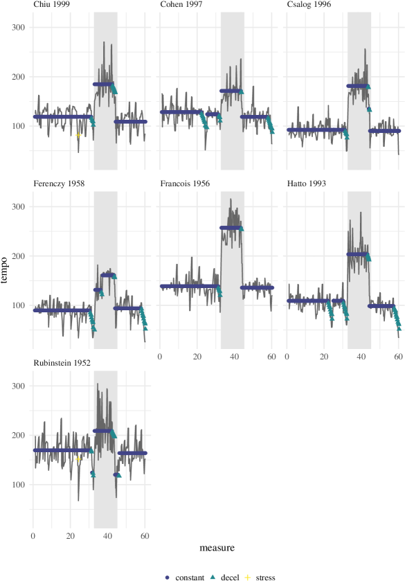
Figure 17: Performances in the first cluster.

Recordings in the second cluster (Figure 18) tend to transition quickly between states, especially constant tempo and slowing down accompanied by frequent transitory emphases. The probability of remaining in state 1 is the lowest for this cluster while the probability of entering state 2 from state 1 is the highest. The acceleration state is visited only rarely.

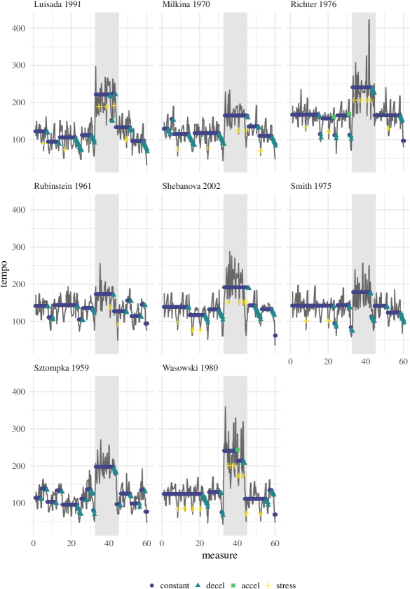
Figure 18: Performances in the second cluster.

Cluster three (Figure 19) is somewhat like cluster one in that performers tend to stay in state 1 for long periods of time, but they transition more quickly from state 3 back to state 1. They also use state 4 frequently whereas cluster one did not. They also tend to have very large tempo contrasts between the A and B sections.

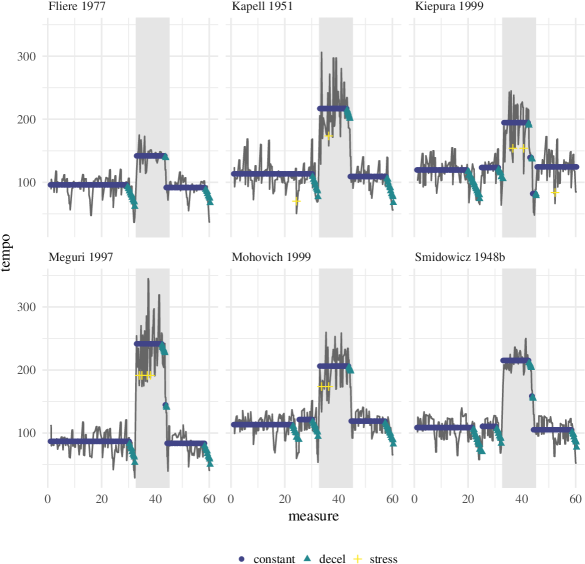
Figure 19: Performances in the third cluster.

Cluster four (Figure 20) has both faster average tempos and more variability from one period of constant tempo to the next. State 4 is rare, with fast constant tempo changes that persist for small amounts of time tending to reflect note emphases.

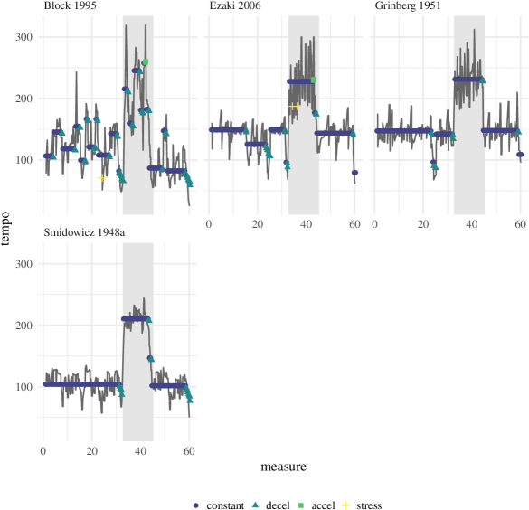
Figure 20: Performances in the fourth cluster.

The remaining performances are relatively different from all other performances (Figure 21. If the distance to the third closest performances exceeded 0.35, then the performance was grouped with “other”. Essentially, these recordings had at most one similar recording while the four other clusters contained at least 4.

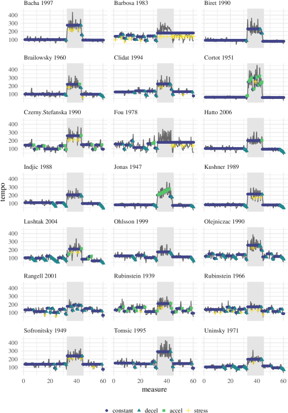
Figure 21: Performances in the “other” cluster.

References

- Anderson and Moore (1979) Anderson, B. D., and Moore, J. B. (1979), Optimal filtering, Prentice-Hall, Englewood Cliffs, NJ.
- Andrieu et al. (2010) Andrieu, C., Doucet, A., and Holenstein, R. (2010), “Particle Markov chain Monte Carlo methods,” Journal of the Royal Statistical Society. Series B, Statistical Methodology, 72(2), 1–33.
- Ariza (2005) Ariza, C. (2005), “Navigating the landscape of computer aided algorithmic composition systems: a definition, seven descriptors, and a lexicon of systems and research.” in Proceedings of International Computer Music Conference.
- Arzt and Widmer (2015) Arzt, A., and Widmer, G. (2015), “Real-time music tracking using multiple performances as a reference.” in International Society for Music Information Retrieval (ISMIR), pp. 357–363.
- Bernstein (2005) Bernstein, L. (2005), Young People’s Concerts, Amadeus Press, Pompton Plains, NJ.
- Bisiani (1992) Bisiani, R. (1992), “Beam search,” in Encyclopedia of Artificial Intelligence, ed. S. Shapiro, John Wiley and Sons, 2nd edn.
- Block et al. (2011) Block, B. A., Jonsen, I. D., Jorgensen, S. J., Winship, A. J., Shaffer, S. A., Bograd, S. J., Hazen, E. L., Foley, D. G., Breed, G., Harrison, A.-L., et al. (2011), “Tracking apex marine predator movements in a dynamic ocean,” Nature, 475(7354), 86.
- Boulanger-Lewandowski et al. (2012) Boulanger-Lewandowski, N., Bengio, Y., and Vincent, P. (2012), “Modeling temporal dependencies in high-dimensional sequences: Application to polyphonic music generation and transcription,” in Proceedings of the 29th International Conference on Machine Learning, Edinburgh, Scotland, UK.
- Burkholder et al. (2014) Burkholder, J. P., Grout, D. J., and Palisca, C. V. (2014), A History of Western Music, WW Norton & Company, 9th edn.
- CHARM (2009) CHARM (2009), “Centre for the History and Analysis of Recorded Music,” Online; accessed 12 March 2019.
- Collins (2016) Collins, N. (2016), “A funny thing happened on the way to the formula: Algorithmic composition for musical theater,” Computer Music Journal, 40(3), 41–57.
- Cont (2010) Cont, A. (2010), “A coupled duration-focused architecture for real-time music-to-score alignment,” IEEE Transactions on Pattern Analysis and Machine Intelligence, 32(6), 974–987.
- Cont et al. (2007) Cont, A., Schwarz, D., Schnell, N., and Raphael, C. (2007), “Evaluation of real-time audio-to-score alignment,” in International Symposium on Music Information Retrieval (ISMIR).
- Craven and Wahba (1978) Craven, P., and Wahba, G. (1978), “Smoothing noisy data with spline functions,” Numerische Mathematik, 31(4), 377–403.
- Dannenberg (1985) Dannenberg, R. (1985), “An on-line algorithm for real-time accompaniment,” in Proceedings of the 1984 International Computer Music Conference, pp. 193–198, International Computer Music Association.
- Dannenberg and Raphael (2006) Dannenberg, R. B., and Raphael, C. (2006), “Music score alignment and computer accompaniment,” Communications of the ACM, 49(8), 38–43.
- Dror et al. (2012) Dror, G., Koenigstein, N., Koren, Y., and Weimer, M. (2012), “The Yahoo! Music Dataset and KDD-Cup’11,” in KDD Cup, pp. 8–18.
- Durbin and Koopman (2001) Durbin, J., and Koopman, S. (2001), Time Series Analysis by State Space Methods, Oxford Univ Press, Oxford.
- Durbin and Koopman (1997) Durbin, J., and Koopman, S. J. (1997), “Monte Carlo maximum likelihood extimation for non-Gaussian state space models,” Biometrika, 84(3), 669–684.
- Earis (2007) Earis, A. (2007), “An algorithm to extract expressive timing and dynamics from piano recordings,” Musicae Scientiae, 11(2), 155–182.
- Earis (2009) Earis, A. (2009), “Mazurka in F Major, Op. 68, No. 3,” accessed 12 March 2019.
- Eddelbuettel (2013) Eddelbuettel, D. (2013), Seamless R and C++ Integration with Rcpp, Springer, New York.
- Fearnhead and Clifford (2003) Fearnhead, P., and Clifford, P. (2003), “On-line inference for hidden markov models via particle filters,” Journal of the Royal Statistical Society: Series B (Statistical Methodology), 65(4), 887–899.
- Flossmann et al. (2013) Flossmann, S., Grachten, M., and Widmer, G. (2013), “Expressive performance rendering with probabilistic models,” in Guide to Computing for Expressive Music Performance, pp. 75–98, Springer.
- Forsén et al. (2013) Forsén, S., Gray, H. B., Lindgren, L. O., and Gray, S. B. (2013), “Was something wrong with Beethoven’s metronome?” Notices of the AMS, 60(9).
- Fox et al. (2011) Fox, E. B., Sudderth, E. B., Jordan, M. I., and Willsky, A. S. (2011), “A sticky HDP-HMM with application to speaker diarization,” The Annals of Applied Statistics, 5, 1020–1056.
- Fuh (2006) Fuh, C.-D. (2006), “Efficient likelihood estimation in state space models,” Annals of Statistics, 34(4), 2026–2068.
- Galili et al. (2017) Galili, T., O’Callaghan, A., Sidi, J., and Sievert, C. (2017), “heatmaply: an R package for creating interactive cluster heatmaps for online publishing,” Bioinformatics, 34(9), 1600–1602.
- Ghahramani and Hinton (2000) Ghahramani, Z., and Hinton, G. E. (2000), “Variational learning for switching state-space models,” Neural Computation, 12(4), 831–864.
- Golub et al. (1979) Golub, G. H., Heath, M., and Wahba, G. (1979), “Generalized cross-validation as a method for choosing a good ridge parameter,” Technometrics, 21(2), 215–223.
- Gu and Raphael (2012) Gu, Y., and Raphael, C. (2012), “Modeling piano interpretation using switching Kalman filter.” in International Society for Music Information Retrieval (ISMIR), pp. 145–150.
- Hadjeres et al. (2017) Hadjeres, G., Pachet, F., and Nielsen, F. (2017), “DeepBach: a steerable model for Bach chorales generation,” in Proceedings of the 34th International Conference on Machine Learning, eds. D. Precup and Y. W. Teh, vol. 70 of Proceedings of Machine Learning Research, pp. 1362–1371, International Convention Centre, Sydney, Australia, PMLR.
- Hamilton (2011) Hamilton, J. (2011), “Calling recessions in real time,” International Journal of Forecasting, 27, 1006–126.
- Harvey (1990) Harvey, A. C. (1990), Forecasting, structural time series models and the Kalman filter, Cambridge University Press.
- Kallberg (1996) Kallberg, J. (1996), Chopin at the boundaries: Sex, history, and musical genre, Harvard University Press.
- Kalman (1960) Kalman, R. E. (1960), “A new approach to linear filtering and prediction problems,” Journal of Basic Engineering, 82(1), 35–45.
- Kim and Nelson (1998) Kim, C., and Nelson, C. (1998), “Business cycle turning points, a new coincident index, and tests of duration dependence based on a dynamic factor model with regime switching,” Review of Economics and Statistics, 80(2), 188–201.
- Kim (1994) Kim, C.-J. (1994), “Dynamic linear models with markov-switching,” Journal of Econometrics, 60(1–2), 1–22.
- Kim et al. (2009) Kim, S.-J., Koh, K., Boyd, S., and Gorinevsky, D. (2009), “ trend filtering,” SIAM Review, 51(2), 339–360.
- Kitagawa (1987) Kitagawa, G. (1987), “Non-Gaussian state-space modeling of nonstationary time series,” Journal of the American Statistical Association, 82, 1032–1041.
- Kitagawa (1996) Kitagawa, G. (1996), “Monte Carlo filter and smoother for non-Gaussian nonlinear state space models,” Journal of Computational and Graphical Statistics, , 1–25.
- Koyama et al. (2010) Koyama, S., Pérez-Bolde, L. C., Shalizi, C. R., and Kass, R. E. (2010), “Approximate methods for state-space models,” Journal of the American Statistical Association, 105(489), 170–180.
- Lang and Freitas (2005) Lang, D., and Freitas, N. D. (2005), “Beat tracking the graphical model way,” in Advances in Neural Information Processing Systems, pp. 745–752, Cambridge, MA, MIT press.
- Lang et al. (2017) Lang, M., Bischl, B., and Surmann, D. (2017), “batchtools: Tools for R to work on batch systems,” The Journal of Open Source Software, 2(10), 135.
- McFee and Lanckriet (2011) McFee, B., and Lanckriet, G. (2011), “Learning multi-modal similarity,” Journal of Machine Learning Research, 12, 491–523.
- Patterson et al. (2008) Patterson, T. A., Thomas, L., Wilcox, C., Ovaskainen, O., and Matthiopoulos, J. (2008), “State–space models of individual animal movement,” Trends in ecology & evolution, 23(2), 87–94.
- R Core Team (2019) R Core Team (2019), R: A Language and Environment for Statistical Computing, R Foundation for Statistical Computing, Vienna, Austria.
- Raphael (2002) Raphael, C. (2002), “A hybrid graphical model for rhythmic parsing,” Artificial Intelligence, 137(1), 217–238.
- Raphael (2010) Raphael, C. (2010), “Music plus one and machine learning,” in Proceedings of the 27th International Conference on Machine Learning (ICML-10), eds. J. Fürnkranz and T. Joachims, pp. 21–28, Haifa, Israel.
- Rauch et al. (1965) Rauch, H. E., Striebel, C., and Tung, F. (1965), “Maximum likelihood estimates of linear dynamic systems,” AIAA journal, 3(8), 1445–1450.
- Ren et al. (2010) Ren, L., Dunson, D., Lindroth, S., and Carin, L. (2010), “Dynamic nonparametric Bayesian models for analysis of music,” Journal of the American Statistical Association, 105, 458–472.
- Roberts et al. (2018a) Roberts, A., Engel, J., Raffel, C., Hawthorne, C., and Eck, D. (2018a), “A hierarchical latent vector model for learning long-term structure in music,” in Proceedings of the 35th International Conference on Machine Learning, eds. J. Dy and A. Krause, vol. 80 of Proceedings of Machine Learning Research, pp. 4364–4373, Stockholmsmässan, Stockholm Sweden, PMLR.
- Roberts et al. (2018b) Roberts, A., Hawthorne, C., and Simon, I. (2018b), “Magenta.js: A javascript api for augmenting creativity with deep learning,” in Joint Workshop on Machine Learning for Music (ICML).
- Schedl et al. (2014) Schedl, M., Gómez, E., Urbano, J., et al. (2014), “Music information retrieval: Recent developments and applications,” Foundations and Trends® in Information Retrieval, 8(2–3), 127–261.
- Sturm et al. (2019) Sturm, B. L., Ben-Tal, O., Monaghan, Ú., Collins, N., Herremans, D., Chew, E., Hadjeres, G., Deruty, E., and Pachet, F. (2019), “Machine learning research that matters for music creation: A case study,” Journal of New Music Research, 48(1), 36–55.
- Thickstun et al. (2017) Thickstun, J., Harchaoui, Z., and Kakade, S. M. (2017), “Learning features of music from scratch,” in International Conference on Learning Representations (ICLR).
- Tibshirani (2014) Tibshirani, R. J. (2014), “Adaptive piecewise polynomial estimation via trend filtering,” Annals of Statistics, 42, 285–323.
- van den Oord et al. (2013) van den Oord, A., Dieleman, S., and Schrauwen, B. (2013), “Deep content-based music recommendation,” in Advances in Neural Information Processing Systems 26, eds. C. J. C. Burges, L. Bottou, M. Welling, Z. Ghahramani, and K. Q. Weinberger, pp. 2643–2651, Curran Associates, Inc.
- Vercoe (1984) Vercoe, B. (1984), “The synthetic performer in the context of live performance,” in Proceedings of the 1984 International Computer Music Conference, pp. 199–200, International Computer Music Association.
- Wahba (1990) Wahba, G. (1990), Spline models for observational data, vol. 59 of CBMS-NSF Regional Conference Series in Applied Mathematics, Society for Industrial and Applied Mathematics (SIAM), Philadelphia, PA.
- Whiteley et al. (2010) Whiteley, N., Andrieu, C., and Doucet, A. (2010), “Efficient Bayesian inference for switching state-space models using discrete particle Markov chain Monte Carlo methods,” Tech. Rep. 10:04, Bristol University.
- Wickham (2016) Wickham, H. (2016), ggplot2: Elegant graphics for data analysis, Springer, 2nd edn.
- Wickham (2017) Wickham, H. (2017), tidyverse: Easily Install and Load the ’Tidyverse’, R package version 1.2.1.