Observational constraints on the magnetic field of the bright transient Be/X-ray pulsar SXP 4.78

Abstract

We report results of the spectral and timing analysis of the Be/X-ray pulsar SXP 4.78 using the data obtained during its recent outburst with NuSTAR, Swift, Chandra and NICER observatories. Using an overall evolution of the system luminosity, spectral analysis and variability power spectrum we obtain constraints on the neutron star magnetic field strength. We found a rapid evolution of the variability power spectrum during the rise of the outburst, and absence of the significant changes during the flux decay. Several low frequency quasi-periodic oscillation features are found to emerge on the different stages of the outburst, but no clear clues on their origin were found in the energy spectrum and overall flux behaviour. We use several indirect methods to estimate the magnetic field strength on the neutron star surface and found that most of them suggest magnetic field $B\lesssim 2\times 10^{12}$ G. The strictest upper limit comes from the absence of the cyclotron absorption features in the energy spectra and suggests relatively weak magnetic field $B<6\times 10^{11}$ G.

1 Introduction

Discovery of pulsating ultra-luminous X-ray sources (Bachetti et al., 2014; Fürst et al., 2016; Israel et al., 2017a, b; Rodríguez Castillo et al., 2019) unambiguously showed that neutron stars (NSs) can exceed their Eddington limit by orders of magnitudes. One of the necessary condition for existence of such a high luminosity was proposed to be a superstrong magnetar-like magnetic field which may significantly reduce the scattering cross-section (Mushtukov et al., 2015; Tong, 2015). The magnetic field also regulates the mass accretion rate reaching the NS surface and therefore the limiting luminosity (Lipunov, 1982; Chashkina et al., 2019). Bright transient X-ray pulsars (XRPs) can be considered as a connecting link between a well-studied sample of moderately bright sources with known magnetic field and ultra-luminous X-ray pulsars. In order to reveal this possible link one need to determine magnetic field strength in the brightest representatives of the XRPs family. Do ultra-luminous X-ray pulsars form a new class of systems or they are usual high mass X-ray binaries (HMXBs), occasionally accreting at the super-Eddington rate, is still an open question.

To approach answering this question it is important to study usual XRPs at high luminosities. A significant fraction of such systems appear to be binaries with Be star companion (Walter et al., 2015) at highly elliptical orbits, referred to as Be X-ray binaries or BeXRBs. They are transient systems, demonstrating different types of outbursts (see review by Reig, 2011). During so-called Type II outbursts these systems often reach or even exceed the Eddington limit (see, e.g., Tsygankov et al., 2017b, 2018), which make them good candidates to search connections with ULX pulsars and to study the accretion at high rates.

SXP 4.78 (or XTE J0052$-$723) was discovered by the RXTE observatory during scanning observations of the Small Magellanic Cloud in December 2000 (Corbet et al., 2001). These observations revealed a bright X-ray source with coherent pulsations at $\sim 4.782$ s and a double-peaked pulse profile (Laycock et al., 2003). Four more outbursts from this source were detected by RXTE  (Klus et al., 2014) during which its luminosity reached $\sim 10^{38}$ erg s^-1 (Laycock et al., 2003), assuming the distance of 60.3 kpc. Taking into account such a transient behaviour the source was suggested to be a BeXRB, although it was impossible to achieve a precise localization with these scanning observations and to determine its optical counterpart. There were several attempts to estimate the magnetic field strength of SXP 4.78, but an insufficient sensitivity, low number of observations and neglect of the orbital motion lead to a wide range of possible values of the magnetic filed in the range $10^{11}$–$4\times 10^{13}$ G (Laycock et al., 2003; Klus et al., 2014; Shi et al., 2015).

The source once again went into the outburst in November 2018 and was detected by the Swift observatory (Coe et al., 2018). A precise localization of SXP 4.78 obtained with the XRT telescope on board of Swift allowed an identification of its optical counterpart – the bright star [M2002] SMC 20671. Monageng et al. (2019) investigated optical spectra of this star and deduced its class as B0.5-IV-V with a strong emission H${\alpha}$ line thereby confirming a Be-nature of the system. These authors inspected also the long-term optical variability of the object with the OGLE project data and found no clear signatures of the orbital period. The outburst was observed extensively by many orbital X-ray observatories and telescopes providing a vast amount of data in the broad energy band (0.2–78 keV). Based on the NuSTAR observation on 2018 Nov 15-17, Antoniou et al. (2018) reported an evidence for a cyclotron resonance scattering feature (CRSF) at $\sim 10$ keV, which is still unconfirmed.

In this paper, based on the data from Swift, NICER, NuSTAR, XMM-Newton, and Chandra observatories, we carried out comprehensive timing and spectral analysis of the source properties during the 2018 super-Eddington Type II outburst with the main aim to constrain the unknown strength of the magnetic field in this system. In Section 2 we describe the available data and their reduction. Section 3 presents the results of the timing analysis and magnetic field estimations from the propeller effect and power spectra. In Section 4 we investigate the X-ray spectrum of the source and present a search for the cyclotron line. The summary of results obtained with different methods is provided in Section 5.

2 Observations and data reduction

After the detection of the new X-ray outburst of SXP 4.78 by the Swift observatory, it was frequently monitored with NICER and Swift/XRT, counting up 69 and 34 observations, correspondingly, distributed over 2018 Nov – 2019 Feb. Also, there were three long NuSTAR pointings near the outburst peak. At the late stage of the outburst we initiated the Chandra Target-of-Opportunity observation (PI Lutovinov), which was performed on 2019 March 1. To estimate the lowest possible flux of SXP 4.78, we used also archived observations with the XMM-Newton observatory, performed in 2007-2016.

Depending on the capabilities of instruments, these data were utilized for spectral and/or timing analysis. Whenever energy spectra are obtained they were grouped to have at least 30 counts per bin with grppha tool. The final data analysis (timing and spectral) was performed with the heasoft 6.25 software package. All uncertainties are quoted at the $1\sigma$ confidence level, if not stated otherwise.

2.1 NuSTAR data

The NuSTAR space observatory consists of two identical X-ray telescope modules, each equipped with independent mirror systems and focal plane detector units, also referred to as FPMA and FPMB (Harrison et al., 2013). It provides X-ray imaging, spectroscopy and timing in the energy range of 3–79 keV with the angular resolution of 18″ (FWHM) and spectral resolution of 400 eV (FWHM) at 10 keV.

Table 1: NuSTAR observations of SXP 4.78 and measured pulse periods, and quasi simultaneous Swift/XRT observations.

ObsID	Date	Exposure, ks	Period, s
NuSTAR
30361003002	2018-11-15	74.5	$4.781607\pm 0.000005$
30361003004	2018-11-24	38.3	$4.781671\begin{subarray}{c}+0.000001\\ -0.000005\end{subarray}$
30361003006	2018-11-27	73.2	$4.781656\pm 0.000001$
Swift
00010977003	2018-11-16	4.9
00010977004	2018-11-25	6.9
00031998011	2018-11-27	5.9

NuSTAR performed three observations of SXP 4.78 during the outburst, all were held near its maximum (see Table  1). Hereafter we refer to these observations as first, second and third ones based on their chronological order. To process the NuSTAR data we used the standard nustardas 1.8.0 software as distributed with the heasoft 6.25 package and the CALDB version 20181030. The standard lcmath tool was used to combine the light curves of the NuSTAR modules to improve statistics for the timing analysis. Source data were extracted from a circular region with radius of 90″, centered at its position. Background data were extracted using a region of an equivalent area away from the source position. Observational data have no signs of a contamination by a stray-light or ghost rays.

2.2 NICER data

The Neutron star Interior Composition Explorer (NICER) is an International Space Station payload consisting of 56 "concentrator" optics above silicon drift detectors operating in the 0.2–12 keV energy band (Gendreau et al., 2016). It provides more than 2000 cm² effective area in the soft X-rays, excellent timing capabilities and CCD-like spectral resolution. Due to the availability of the NuSTAR and Swift/XRT data, well calibrated and suitable for the broadband spectral analysis, we used the NICER data only for the analysis of the temporal properties of the source.

The data reduction was performed with the standard nicerdas software (V005). We applied a barycentric correction to all cleaned event lists. As it was discussed by Prigozhin et al. (2016) so-called ‘hard tails’, produced by the high-energy particles, can be observed in the NICER energy spectra. This component of the spectrum introduces an additional stochastic noise which has a complex shape in the power spectra (see, e.g. Sanna et al., 2018). In order to reduce the impact of this noise in our data we applied additional filtering criterion to the NICER data, following Bult et al. (2018). Initially, we build a light curve in the 1200–1500 PI channels range (corresponding to 12–15 keV energy band, where the instrument has negligible effective area). After that new good time intervals, including only those part of the light curve with the count rate below 1 count per second, were created. Note, that this procedure usually leads to the loss of $\sim$10 per cent of the exposure time in each individual observation.

The source was observed 69 times in the period from 2018 November 10 to 2019 March 12 (ObsIDs 12004101[01–69]). For our analysis we used all these data, excluding observations with ObsIDs 1200410110 and 1200410141 for which we could not make the barycentric correction. After the filtering we obtained 90.5 ks of the total exposure. For the following analysis we use events registered in 50–800 PI channels corresponding to the 0.5–8 keV energy band.

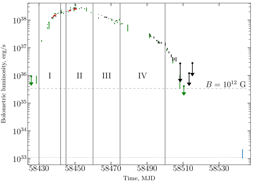
Figure 1: Evolution of the SXP 4.78 bolometric luminosity during the outburst, as measured by Swift/XRT (green points with error bar), NuSTAR (red) and NICER (black). The Chandra observations in the quiescent state is shown by the blue error bar. The dashed horizontal line represents the critical luminosity at which the source should switch to the ‘propeller mode’ for the magnetic field strength of $10^{12}$ G. The dotted horizontal line demonstrates the upper limit for the source luminosity derived from XMM-Newton data obtained in 2009 (ObsID. 0601210701).

2.3 Swift data

The Neil Gehrels Swift Observatory (Gehrels et al., 2004) carries several instruments including the glazing mirror X-ray telescope (XRT) allowing to perform imaging, spectral and timing analysis in soft X-rays (Burrows et al., 2000). The telescope can operate in the imaging and timing modes. SXP 4.78 was observed 35 times since its first detection on 2018 November 9 till the last detection on 2019 February 24. A median exposure of the single observation was about 1 ks. Only five of these observations were performed in windowed timing mode, therefore we used Swift/XRT data only for spectral analysis. The spectra were produced by the online tool (Evans et al., 2009). The data analysis was restricted to the 0.8–9 keV energy band.

2.4 Chandra data

At the late stage, when the source became too weak for Swift/XRT, we employed the Chandra observatory to determine the source state and measure its flux. The observation was carried out on 2019 Mar 1 (ObsId. 22095). The standard ciao package with latest calibration files was used to analyse these data. First, the obtained data were reprocessed to produce the sky map in the 0.5–7 keV energy band. No significant background variations over the course of observation were found. Usage of the wavdetect procedure yields a 2.7$\sigma$ detection of the source at 0.44″ away from the optical counterpart of SXP 4.78. This offset is consistent both with measured uncertainties on the source position and the typical Chandra astrometric precision.

2.5 XMM-Newton data

The field of SXP 4.78 was observed with the XMM-Newton observatory three times in the past, but the source was never detected. Nevertheless the knowledge of the source flux in the quiescent state is important for understanding the presence of the propeller regime and estimation of the magnetic field. Therefore we used the FLIX service (Carrera et al., 2007) to estimate the $4\sigma$ upper limits on the source flux in these observations. The obtained limits are presented in Table 2.

Table 2: XMM-Newton observations of SXP 4.78

ObsID	Date	Exposure	Flux upper limit
		ks	erg s-1 cm${{}^{-}2}$
0500980101	2007-06-23	24	$7.0\times 10^{-15}$
0601210701	2009-09-27	37	$2.5\times 10^{-15}$
0793182901	2016-10-14	35	$3.2\times 10^{-15}$

2.6 Bolometric correction

The 2018 outburst of SXP 4.78 was well covered by monitoring observations with Swift/XRT and NICER instruments, allowing us for the first time to examine its profile in details from the rise to the decline. It is necessary to note that these monitoring programs were performed in the X-ray range with energies not exceeding 10–12 keV, but for estimations of physical properties of the source (e.g. the magnetic field) we need to know its bolometric luminosity (we consider it as a luminosity in the 0.1–100 keV energy band). To reconstruct the broad-band spectrum of the source and to calculate the bolometric correction we used three NuSTAR (and nearly simultaneous Swift/XRT) observations as reference points (see Section 4 for details). It was found that the bolometric correction from the luminosity in the 0.5–8 keV energy band slightly varied as $K_{\rm bol}\simeq(2.2-2.4)$, but the spectral shape remained approximately the same. Therefore, in the following as a bolometric correction we adopted $K_{\rm bol}=2.3$.

3 Timing analysis

As it was mentioned in the introduction, the RXTE data allowed measurements of some timing properties of SXP 4.78 (pulsations, pulse profiles, etc.). However, the small number of the available observations prevented in depth timing studies of the source, especially at low luminosities. In this section, we perform the timing analysis of newly available data in the X-ray band, accumulated with NuSTAR and NICER during the recent outburst of the source. Swift/XRT data were used also in order to trace the overall evolution of the source luminosity during the outburst.

3.1 Long term temporal behaviour

The overall outburst profile is shown in Fig. 1. The first detection corresponds to 2018 Nov 9 (MJD 58431) when the source was revealed by Swift/XRT with the bolometric luminosity of $L_{\rm bol}\simeq 7\times 10^{35}$erg s^-1. In the beginning of the outburst the source underwent fast rise, increasing its luminosity by a hundred times over nine days and reaching $10^{38}$erg s^-1. Then the growth rate was decreased and in the consecutive dozen days the luminosity has increased from $10^{38}$ to $2.5\times 10^{38}$ erg s^-1. After reaching the maximum a gradual decay started, lasting for approximately 50 days. As soon as the luminosity has decreased down to $L_{\rm bol}\simeq 2\times 10^{37}$ erg s^-1, a nearly power-law decay switched to a faster decay. Eventually, the source was not detected by Swift/XRT with the upper limit of $L_{\rm bol}<4.1\times 10^{35}$ erg s^-1($2\sigma$) on 2019 Jan 27 (MJD 58510) during a long ($\simeq 4$ ks) observation.

Such a behaviour is typical for fast rotating NSs in transient BeXRBs and indicates the transition of the system to the propeller regime (Illarionov & Sunyaev, 1975). Therefore, after the beginning of the rapid flux decay we initiated the Chandra ToO observation with the main aim to observe the source in the quiescence state. The observation was performed on 2019 Mar 1. Despite only the marginal detection of the source it still had an important scientific significance. The source count rate in the 0.5–7 keV energy band was estimated with the srcflux tool of the ciao package as $3.7\times 10^{-4}$ s^-1 with the 90 per cent confidence interval being (1.5–7.4)$\times 10^{-4}$ s^-1. Assuming a blackbody spectrum with the temperature of $kT=0.5$ keV, that is expected and observed for sources in the propeller regime (see, e.g., Tsygankov et al., 2016; Wijnands & Degenaar, 2016), and the absorption column of $2\times 10^{21}$ cm^-2 (Kalberla et al., 2005), we estimated an unabsorbed source flux of $3.7\times 10^{-15}$erg s^-1 cm^-2 and the corresponding intrinsic luminosity of $L_{q}\simeq 1.6\times 10^{33}$erg s^-1 for the distance of 60.3 kpc. Such a luminosity agrees well with usual values for HMXBs in the propeller state (Tsygankov et al., 2016; Wijnands & Degenaar, 2016; Tsygankov et al., 2017a; Lutovinov et al., 2017, 2019).

As it was mentioned above, the source was traced until the Swift/XRT non-detection at the luminosity of $L_{\rm bol}\lesssim 4.1\times 10^{35}$ erg s^-1 (Fig. 1). Using this value as the upper limit on the critical luminosity of the transition to the propeller regime we can constrain the NS magnetic field of SXP 4.78 as (see, for example, Tsygankov et al., 2016):

$$B_{\rm 12}\simeq 0.5L_{\rm 37}^{1/2}P^{7/6}M_{\rm 1.4}^{1/3}R_{6}^{-5/2}k^{-7/4},$$ (1)

where $B_{\rm 12}$ is the magnetic field strength in 10¹² G, $L_{\rm 37}$ is the luminosity in $10^{37}$erg s^-1, $P$ is the spin period in seconds, $M_{\rm 1.4}$ is the NS mass in units of 1.4M_⊙, $R_{6}$ is the NS radius in units of $10^{6}$ cm, and $k$ is the ratio of the magnetospheric radius to the Alfvén one, usually taken as 0.5 (Campana et al., 2018). Substituting measured values for the source luminosity and the pulse period, and using current results of the NS radius estimations $R_{6}=1.2$ (Suleimanov et al., 2017b, a; Nättilä et al., 2017) we can estimate an upper limit on the magnetic field strength as $B\lesssim 1.5\times 10^{12}$ G.

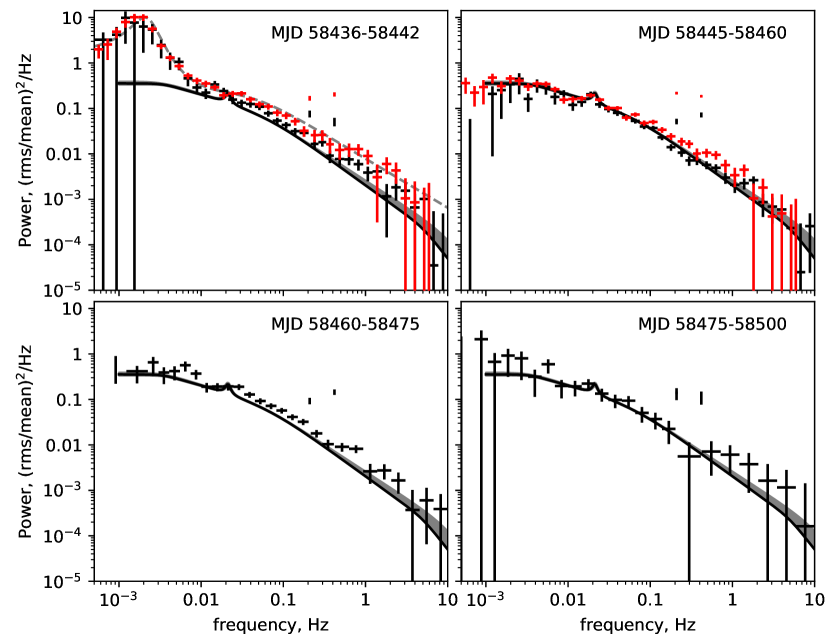
Figure 2: Power spectra of SXP 4.78, obtained with NICER (black crosses) and NuSTAR (red crosses) in four epochs of the outburst (see text and Fig. 1). The black line represents the broken power-law model, which fits the NICER data in the epoch II (top right panel). The grey dashed line on the top left panel shows the band-limited noise model with an additional Lorentzian introduced to describe the low-frequency QPO.

3.2 Power spectrum

Figure 3: Power spectrum of SXP 4.78 at low frequencies obtained with NICER and NuSTAR in the epoch II (MJD 58445–58460).

Power spectra of accreting systems can provide important information about the geometry and properties of the accretion disc. In the broad frequency range, the power spectra can be described by a sum of several power-law or broad Lorentzian components (Reig, 2008). At low frequencies, the power spectrum is usually a white noise $P(f)=const$, transiting to the $P(f)\propto f^{-1}$ at higher frequencies. The $P(f)\propto f^{-1}$ segment of the power spectrum is thought to be produced by perturbations propagating in the accretion disc (Lyubarskii, 1997). Above a certain break frequency it transits to even steeper power law $P(f)\propto f^{-2}$. Revnivtsev et al. (2009) suggested that this break frequency corresponds to a Keplerian frequency at the inner edge of the magnetically truncated accretion disc. Thus the detection of such a break in the power spectrum of X-ray pulsars and its evolution with the source luminosity can give an independent estimate of the magnetic field strength in the system (Revnivtsev et al., 2009).

In the following, we investigate the variability properties of SXP 4.78 in terms of its power spectrum and describe it with a combination of broad noise components and coherent pulsations. Firstly, we analysed power spectra of each separate NuSTAR and NICER observation in the 3–78 and 0.5–8 keV energy bands, respectively. We found, that during first twelve days of the outburst the power spectrum had a form of a broken power-law continuum (usually referred to as band-limited noise) and a broad hump-like feature at low frequencies ($5\times 10^{-4}$–$5\times 10^{-3}$ Hz). The presence of the excessive low frequency variability was reported earlier by Guillot et al. (2018) based on the first portion of the NICER data. Interestingly, this feature disappears as the outburst evolves and the luminosity increases. Therefore, in order to measure the power spectrum of SXP 4.78 with a good accuracy and to trace its evolution over the outburst, we split all available data into four epochs (Fig 1): (I) beginning of the outburst (MJD 58436–58442), (II) near the outburst maximum (MJD 58445–58460), (III) slow decay (MJD 58460–58475) and (IV) exponential decay (MJD 58475–58500), and reconstructed power spectra for each of them (Fig. 2).

First, it should be noted that the power spectra obtained from NuSTAR and NICER data are in good agreement with each other for epochs I and II. Second, the power spectra in epochs II, III and IV can be described with a single zero-centered Lorentzian, representing a broad noise component, with narrow spikes near the pulse frequency and its harmonic (Fig. 2). The low-frequency broad noise does not change its shape and amplitude significantly from epoch to epoch in spite of two orders of magnitude variations in the source flux. The overall amplitude of this noise component in both NuSTAR and NICER energy bands was $14\pm 1$ per cent (rms/mean) and the low-frequency break of the component was measured at $F_{\rm lfbr}=(3.5\pm 0.7)\times 10^{-3}$ Hz.

As noted above, in the power spectrum of epoch I, in addition to the band-limited noise component, the broad hump-like feature at low frequencies is also significantly detected (Fig. 2). The overall power by this excessive variation is $15\pm 2$ per cent (rms/mean). Similar features were observed in a number of BeXRBs at different stages of outbursts (see Reig, 2008) and are known as milliherz quasi-periodic oscillations (mQPO). Shirakawa & Lai (2002) proposed a model of the accretion disc wrapped under the influence of the NS magnetic torque to describe such mQPOs. Authors noted, that the mQPO frequency depends in a complex way on the accretion disc parameters which are hard to determine from the observations. Fortunately, among the systems investigated by Shirakawa & Lai (2002) there is another BeXRB pulsar 4U 0115+63, which demonstrated mQPO at 2 mHz when the system has a similar to SXP 4.78 luminosity ($\approx 9\times 10^{37}$erg s^-1). This pulsar has a pulse period of 3.61 s and known magnetic field strength ($B\approx 1.3\times 10^{12}$ G) due to the cyclotron resonance features found in its spectrum (White et al., 1983). Using a general dependence of the mQPO frequency on the magnetic moment derived in the model of Shirakawa & Lai (2002) $\nu_{\rm QPO}\propto\mu_{30}^{-0.81}$ we can roughly estimate the magnetic field in SXP 4.78 as $B\approx 2\times 10^{12}$ G.

All power spectra of SXP 4.78 at high frequencies approximately follow a power law (Fig. 2) without an obvious presence of the high frequency break, which can be associated with the accretion disc inner edge. If the propagating fluctuations theory is valid, such a break should be located at lower frequencies when BeXRBs are less luminous (Revnivtsev et al., 2009). However, it is easy to show, that the significance of the break detection is larger when the system is bright, because the break frequency decreases with the luminosity slower than the Poisson noise amplitude. Thus, for the power spectrum obtained in the brightest epoch (II) we can constrain $F_{\rm br}>5$ Hz, placing a lower limit on the accretion disc inner radius, and therefore, an upper limit on the magnetic field strength $B<10^{12}$ G.

Finally, in order to investigate the power spectrum of SXP 4.78 in details we used epoch II, which contain two long NuSTAR observations. A large number of photons allowed us to build the power spectrum with the higher resolution (Fig. 3) and found that in line with other components the spectrum has another QPO with the centroid at $(2.12\pm 0.06)\times 10^{-2}$ Hz and relative rms of $1.6\pm 0.2$ per cent (rms/mean). Note that a similar QPO was observed in Cen X-3 (Belloni & Hasinger, 1990), but no model, describing its origin was presented.

3.3 Pulsations

A detailed timing analysis is out of scopes of this paper, therefore we limited ourselves here to only some general information about the temporal properties of the source, derived from the NuSTAR data. First of all, pulsations were clearly detected in all three observations and the pulse period was determined with a high accuracy (see Table 1). Although significant changes of the pulse period are observed, we cannot draw any conclusions about the angular momentum transfer (which also can be used for the magnetic filed estimations, see, e.g., Klus et al. 2014) in this system because of lack of orbital ephemeris.

Previously Laycock et al. (2003) reported a double-peaked pulse profile in the 3–10 keV band. Here we used NuSTAR data to study the dependence of the pulse profile and the pulse fraction with energy. The pulse profile has a double-peaked shape, which does not change strongly with energy. We also did not found any significant evolution of the pulse profile between three NuSTAR observations, therefore only data from the brightest NuSTAR observation (ObsID 30361003006) are presented in Fig. 4.

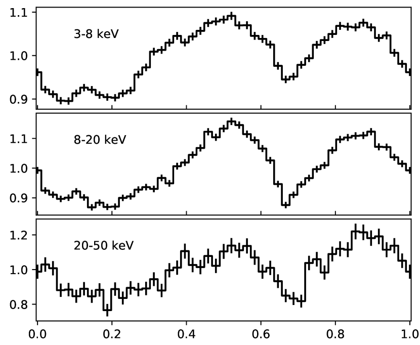
Figure 4: Pulse profile of SXP 4.78 in 3–8, 8–20, and 20–50 keV energy bands according to the NuSTAR data.

The pulsed fraction, calculated as $PF=({F_{\rm max}-F_{\rm min}})/({F_{\rm max}+F_{\rm min}})$, where $F_{\rm max}$ and $F_{\rm min}$ are the maximum and minimum count rates in the profile, respectively, grows with the energy, that is typical for bright X-ray pulsars (Lutovinov & Tsygankov, 2009), and does not evolve significantly from one NuSTAR observation to another (Fig. 5). No additional peculiarities, which previously were detected for several XRPs near the cyclotron line energy (Tsygankov et al., 2007; Ferrigno et al., 2009; Lutovinov & Tsygankov, 2009), were found in the pulsed fraction behaviour of SXP 4.78.

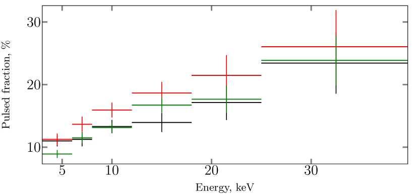
Figure 5: Dependence of the pulsed fraction on energy as measured by the NuSTAR observatory. Observations with ObsID 30361003002, 30361003004 and 30361003006 are shown with the black, red and green crosses, respectively.

4 Spectral analysis

The spectral analysis is by far the most reliable method to estimate the magnetic field strength through the detection of cyclotron absorption lines in spectra of XRPs (see Staubert et al., 2019, for the recent review). Soon after the discovery of SXP 4.78, Laycock et al. (2003) investigated its spectrum with RXTE/PCA and found that it can be well described with the bremsstrahlung emission without any cyclotron absorption features. Recently, a preliminary spectral analysis performed over the first NuSTAR observation (ObsID 30361003002) revealed an evidence for the possible absorption feature at $\sim 10$ keV (Antoniou et al., 2018). Assuming that this spectral feature may appear to be a cyclotron absorption line, authors estimated the magnetic field of the object as $B\approx 0.9\times 10^{12}$ G.

In this section a detailed analysis of the SXP 4.78 X-ray spectrum was performed to examine the possible presence of the cyclotron absorption line and to approximate the source spectrum in the broad energy range in the best way.

4.1 Spectra of SXP 4.78, measured with NuSTAR

The spectrum of SXP 4.78 is typical for accreting XRPs and demonstrates an exponential cutoff at high energies (Fig. 6a). Therefore, as a first step, we attempted to approximate spectra obtained with the NuSTAR observatory, by the power-law model with an exponential cutoff at high energies (cutoffpl in the xspec package) and additional iron emission line at 6.4 keV in the form of the Gaussian. Note, that the same model was used by Antoniou et al. (2018) for the analysis of the first NuSTAR observation (ObsID 30361003002). In agreement with these authors, we found that this model does not describe well the source spectrum. In particular, the residuals demonstrate a wave-like structure with some deficit of photons around 10 keV (Fig. 6b). A formal inclusion to the model of an absorption component in the form of the gabc model at the energy of $E_{\rm cyc}=9.78\pm 0.15$ keV, width of $2.41\pm 0.29$ keV and depth of $\tau_{\rm cyc}=0.083_{-0.014}^{+0.017}$ improves the fit and flattens the residuals (Fig. 6c). Other parameters of the best-fitting model are the photon index $\Gamma=0.55\pm 0.02$, the cutoff energy $E_{\rm cut}=7.80\pm 0.12$ keV, and the iron line energy $E_{\rm Fe}=6.38\pm 0.07$ keV; the iron line width was fixed at 0.3 keV, the value obtained by fitting the spectrum obtained during the third NuSTAR observation (with largest photon statistics) with this parameter free.

At the same time, it is well known that the XRP spectra have a more complex continuum shape than the power law with an exponential cutoff and often several components are required to describe them (Becker & Wolff, 2007; Doroshenko et al., 2012; Tsygankov et al., 2012; Farinelli et al., 2012). We found that this fully applies to the object under study. In particular, an addition to the cutoffpl model of the thermal component in the form of the blackbody model with the temperature of $kT_{\rm BB}\simeq 1.17$ keV improves the fit quality similarly to adding the cyclotron line (Fig. 6d). Moreover, using another continuum model in the form of the comptonized emission (comptt model in the xspec package) allows us to describe the source spectrum much better that with the cutoffpl model without a need to include the cyclotron absorption line (Fig. 6e).

The same analysis was carried out for two other NuSTAR observations of SXP 4.78, and similar results were obtained. Using of the cutoffpl model for the description of the continuum lead again to the wave-like structures in the residuals, which can be compensated by addition of the broad absorption features at energy $E_{\rm cyc}\simeq 11$ and 12.3 keV with depths of $\tau_{\rm cyc}\simeq 0.065$ and 0.14 for observations 30361003004 and 30361003006, respectively. Similarly to the previous case, addition of the blackbody component with the temperature $kT\simeq 1.3$keV or using the comptt continuum model allows us to improve both fits without a need for the cyclotron absorption line.

Summarizing all above we can conclude the relative broadness of the possible absorption feature, its small depth and proximity to the power-law cutoff energy as well as the better approximation of spectra with other models suggests the complexity of the spectral continuum in SXP 4.78, rather than requires the presence of the cyclotron absorption line.

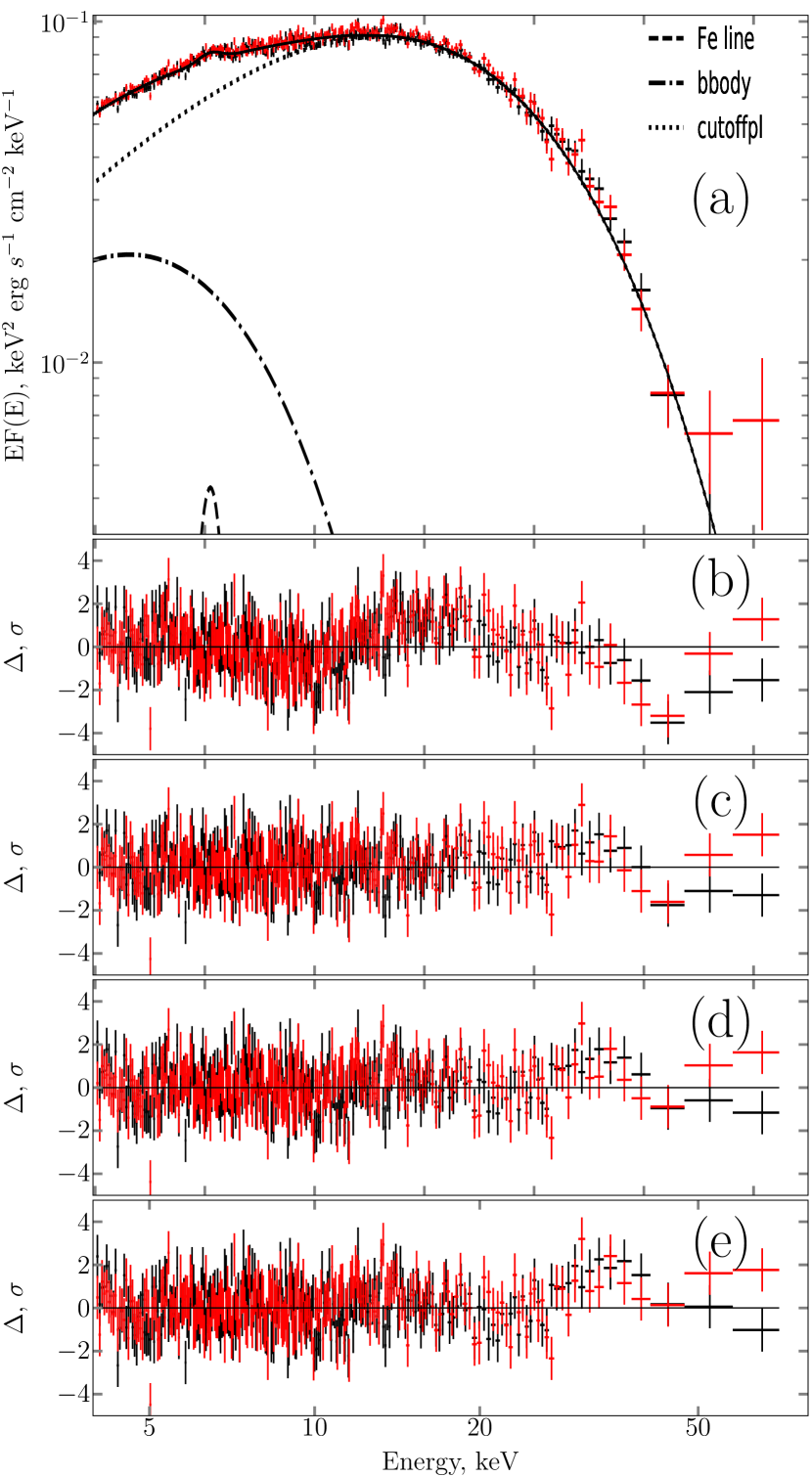
Figure 6: (a) Energy spectrum of SXP 4.78 obtained with the NuSTAR observatory (ObsID 30361003002). The black and red crosses correspond to data from FPMA and FPMB, respectively. The black line shows the best-fitting model. (b-e) Residuals from different models (see text for details). The spectrum and residuals were rebinned in the figure to make deviations more apparent.

4.2 Broadband phase-averaged spectra

To reconstruct the broadband spectra of SXP 4.78 we used all three NuSTAR observations with overlapping the data obtained with Swift/XRT (see Table 1). To take into account the uncertainty in the instrument calibrations, cross-calibration constants between them were included in all spectral models (the $C_{\rm FPMB}$ and $C_{\rm XRT}$ constants correspond to the cross-calibrations of the FPMB module and the XRT telescope to the FPMA module, respectively). Given the lack of sensitive observations at lower energies we fixed the value of the interstellar absorption column at $2\times 10^{21}$ cm^-2, which is typical in the direction to the Small Magellanic Cloud (Kalberla et al., 2005).

Figure 7: (a) The spectrum of SXP 4.78 obtained during the first NuSTAR and simultaneous Swift/XRT observations and unfolded with tbabs (cutoffpl + bbody + bbody + gauss) model. (b) The residuals for such a model without one of the blackbodies. (c) Residuals for the full model.

Table 3: Best-fitting parameters of broad-band spectra of SXP 4.78.

Observation	NUOBS02	NUOBS04	NUOBS06
$N_{\rm H}$, $10^{21}$ cm-2	2 (fixed)	2 (fixed)	2 (fixed)
$\Gamma$	$0.19\pm 0.03$	$0.46\pm 0.03$	$0.32\pm 0.05$
$E_{\rm cut}$, keV	$7.00\pm 0.18$	$7.92\pm 0.12$	$7.56\pm 0.16$
${\rm Norm}_{\rm pl}$, $10^{-3}$	$5.6\pm 0.7$	$12.6\pm 0.7$	$10.4\pm 1.1$
$E_{\rm Fe}$, keV	$6.41\pm 0.07$	$6.49\pm 0.05$	$6.52\pm 0.03$
${\rm Norm}_{\rm Fe}$, $10^{-4}$	$0.87\pm 0.11$	$1.54\pm 0.17$	$1.58\pm 0.14$
EWFe, eV	$39\pm 6$	$46\begin{subarray}{c}+7\\ -5\end{subarray}$	$47\begin{subarray}{c}+5\\ -3\end{subarray}$
$kT_{\rm BB}$, keV	$1.10\pm 0.03$	$1.26\pm 0.02$	$1.32\pm 0.01$
$R_{\rm BB}$, km	$9.2\begin{subarray}{c}+0.3\\ -0.4\end{subarray}$	$8.5\pm 0.4$	$10.1\pm 0.3$
$kT_{\rm BB,s}$, keV	$0.21\pm 0.03$	$0.12\pm 0.2$	$0.21\pm 0.03$
$R_{\rm BB,s}$, km	$148\begin{subarray}{c}+57\\ -48\end{subarray}$	$808\begin{subarray}{c}+887\\ -384\end{subarray}$	$163\begin{subarray}{c}+56\\ -42\end{subarray}$
$C_{\rm FPMB}$	$1.016\pm 0.003$	$1.020\pm 0.003$	$1.021\pm 0.002$
$C_{\rm XRT}$	$1.058\pm 0.015$	$1.000\pm 0.012$	$0.969\pm 0.022$
$\chi^{2}_{\rm red}$	1.003	1.003	1.009
d.o.f.	1715	1692	1669

To describe the SXP 4.78 spectrum in the broad energy range (see Fig. 7a) we used the same models that were considered in Section 4.1. It was found that the comptt model is unable to approximate the broadband spectrum and an addition of the blackbody component is required in the same way as it was required for the cutoffpl model earlier. The performed analysis showed that both combined models, cutoffpl + bbody and comptt + bbody, describe all three broadband spectra equally well, but the cutoffpl model has fewer parameters. Therefore in the following analysis we used the cutoffpl + bbody model as a base one. As before an additional Gaussian component to describe a prominent emission line at 6.4 keV with the fixed width at 0.3 keV was added to the model.

This model approximates the source spectrum quite well, but nevertheless at the residuals panel a very soft excess at energies $<1$ keV is clearly visible (Fig. 7b). Such an excess was previously detected in spectra of several XRPs and was proposed to originate from the material at the inner edge of the accretion disc heated by the central source (Hickox et al., 2004). To describe it we added another blackbody component, which improved the fit quality (Fig. 7c).

Results of the approximation of spectra of SXP 4.78 with the model of phabs*(cutofpl+bbody+bbody+gaus) are presented in Fig.7, corresponding best-fitting parameters are summarized in Table 3. It is clearly seen that the model fits well to all spectra and again shows no systematic deviations which would imply the presence of absorption features. The ‘high-temperature’ blackbody component with $kT_{\rm BB}\simeq 1.1-1.3$ keV is often registered in spectra of Be-XRBs (see, e.g., La Palombara et al., 2012; Tsygankov et al., 2012; Bartlett et al., 2013; Fornasini et al., 2017) and can be connected with the emission of the hot parts of the accretion column or hot spots around these columns, arising by interception of their emission by the surface of the NS (Poutanen et al., 2013). The typical size of the emission region determined from the data agrees well with such an explanation.

The ‘soft’ blackbody component has a temperature in the range of 0.1–0.2 keV consistent with the study by Hickox et al. (2004). Following these authors we can estimate the inner radius of the accretion disc, assuming that it is responsible for this emission and has the height-to-radius ratio $H/R=0.1$. For the first and third NuSTAR observations (where parameters of the soft component are better constrained) we get an estimation of the inner radius as $R_{\rm in}\approx 10^{8}$ cm, that corresponds to the magnetic field strength $B\approx 0.6\times 10^{12}$ G.

4.3 Cyclotron line search in the broad-band spectrum

To test finally the hypothesis of a possible presence of a cyclotron absorption line in the spectra of SXP 4.78, we used an approach proposed by Tsygankov & Lutovinov (2005) and recently updated by Shtykovsky et al. (2017). The best-fitting model was modified by adding the gabs component. After that, the cyclotron line energy $E_{\rm cyc}$ was varied within the 5–55 keV energy range with the step of 0.5 keV. A corresponding line width was varied with the step of 0.5 keV within the range of 1–6 keV (but smaller than $E_{\rm cyc}$/2). For each pair of cyclotron line parameters the position and width were fixed in the gabs model component, the resulting model was used to approximate the spectrum and the confidence interval for the optical depth of the cyclotron line was calculated. As a result, none of the combination of the line energy and its width results in a significant improvement of the fit and only the upper limit for the optical depth $\tau_{\rm cyc}\lesssim 0.06$ (90 per cent confidence interval) was obtained. This upper limit indicates the absence of the cyclotron feature in the 5–55 keV energy range, that allows us to put a limit on the possible strength of the magnetic field on the surface of the NS in SXP 4.78 $B<6\times 10^{11}$ G or $B>6.6\times 10^{12}$ G.

Cyclotron absorption lines often demonstrate variations with the pulse phase (Burderi et al., 2000; Kreykenbohm et al., 2004, see, e.g.), therefore their presence can be more prominent in the phase-resolved spectra. Considering such possibility, we inspected the phase-resolved spectra, but did not find any additional indication in favour of cyclotron absorption lines.

5 Conclusions

In this work we considered temporal and spectral properties of the Be X-ray pulsar SXP 4.78 in order to estimate the strength of the NS magnetic field in this system. Despite the previously reported detection of the cyclotron absorption line at $10.3\pm 0.2$ keV in the NuSTAR spectrum (Antoniou et al., 2018), we found that the majority of spectral models typically used to fit spectra of XRPs do not require an absorption feature in the 5–55 keV energy band. This implies that the magnetic field is either weaker than $0.6\times 10^{12}$ G or stronger than $6.6\times 10^{12}$ G.

A few more indirect methods were applied to further constrain the magnetic field strength. Particularly, the long-term temporal behaviour of the source flux points to the transition of SXP 4.78 to the propeller regime. An upper limit to the transitional luminosity $\sim 4\times 10^{35}$erg s^-1 corresponds to the upper limit on the magnetic field strength $\sim 10^{12}$ G. Another evidence of the relatively weak magnetic field in the source comes from shape of the noise power spectrum. We were able to obtain a lower limit on the break frequency corresponding to the Keplerian frequency at the accretion disc inner edge as $f_{\rm br}>5$ Hz. This frequency corresponds to the magnetospheric radius around $10^{8}$ cm and, hence, the magnetic field lower than $\sim 10^{12}$ G. Similar magnetic field strength was obtained from parameters of the soft blackbody component in the energy spectrum of the pulsar associated with the emission from the inner edge of the accretion disc.

Finally, we were able to discover a millihertz QPO in the power spectrum at $\sim 1.6$ mHz, which may originate from the precession of the magnetically wrapped disc (Shirakawa & Lai, 2002), providing information about the magnetic field strength. Using measured QPO frequency we derived the magnetic field strength of $B\sim 2\times 10^{12}$ G. Summarizing all the above, we can conclude that SXP 4.78 contains a relatively weakly-magnetized NS with the magnetic field strength lower than $10^{12}$ G.

References

- Antoniou et al. (2018) Antoniou V., Zezas A., Hong J., Kennea J., Tomsick J., Haberl F., 2018, The Astronomer’s Telegram, 12234
- Bachetti et al. (2014) Bachetti M., et al., 2014, Nature, 514, 202
- Bartlett et al. (2013) Bartlett E. S., Coe M. J., Ho W. C. G., 2013, MNRAS, 436, 2054
- Becker & Wolff (2007) Becker P. A., Wolff M. T., 2007, ApJ, 654, 435
- Belloni & Hasinger (1990) Belloni T., Hasinger G., 1990, A&A, 230, 103
- Bult et al. (2018) Bult P., et al., 2018, ApJ, 860, L9
- Burderi et al. (2000) Burderi L., Di Salvo T., Robba N. R., La Barbera A., Guainazzi M., 2000, ApJ, 530, 429
- Burrows et al. (2000) Burrows D. N., et al., 2000, in Flanagan K. A., Siegmund O. H., eds, Proc. SPIE Vol. 4140, X-Ray and Gamma-Ray Instrumentation for Astronomy XI. pp 64–75, doi:10.1117/12.409158
- Campana et al. (2018) Campana S., Stella L., Mereghetti S., de Martino D., 2018, A&A, 610, A46
- Carrera et al. (2007) Carrera F. J., et al., 2007, A&A, 469, 27
- Chashkina et al. (2019) Chashkina A., Lipunova G., Abolmasov P., Poutanen J., 2019, A&A, 626, A18
- Coe et al. (2018) Coe M. J., Kennea J. A., Buckley D., Udalski A., 2018, The Astronomer’s Telegram, 12209
- Corbet et al. (2001) Corbet R., Marshall F. E., Markwardt C. B., 2001, IAU Circ., 7562
- Doroshenko et al. (2012) Doroshenko V., Santangelo A., Kreykenbohm I., Doroshenko R., 2012, A&A, 540, L1
- Evans et al. (2009) Evans P. A., et al., 2009, MNRAS, 397, 1177
- Farinelli et al. (2012) Farinelli R., Ceccobello C., Romano P., Titarchuk L., 2012, A&A, 538, A67
- Ferrigno et al. (2009) Ferrigno C., Becker P. A., Segreto A., Mineo T., Santangelo A., 2009, A&A, 498, 825
- Fornasini et al. (2017) Fornasini F. M., Tomsick J. A., Bachetti M., Krivonos R. A., Fürst F., Natalucci L., Pottschmidt K., Wilms J., 2017, ApJ, 841, 35
- Fürst et al. (2016) Fürst F., et al., 2016, ApJ, 831, L14
- Gehrels et al. (2004) Gehrels N., et al., 2004, ApJ, 611, 1005
- Gendreau et al. (2016) Gendreau K. C., et al., 2016, in Space Telescopes and Instrumentation 2016: Ultraviolet to Gamma Ray. p. 99051H, doi:10.1117/12.2231304
- Guillot et al. (2018) Guillot S., et al., 2018, The Astronomer’s Telegram, 12219
- Harrison et al. (2013) Harrison F. A., et al., 2013, ApJ, 770, 103
- Hickox et al. (2004) Hickox R. C., Narayan R., Kallman T. R., 2004, ApJ, 614, 881
- Illarionov & Sunyaev (1975) Illarionov A. F., Sunyaev R. A., 1975, A&A, 39, 185
- Israel et al. (2017a) Israel G. L., et al., 2017a, Science, 355, 817
- Israel et al. (2017b) Israel G. L., et al., 2017b, MNRAS, 466, L48
- Kalberla et al. (2005) Kalberla P. M. W., Burton W. B., Hartmann D., Arnal E. M., Bajaja E., Morras R., Pöppel W. G. L., 2005, A&A, 440, 775
- Klus et al. (2014) Klus H., Ho W. C. G., Coe M. J., Corbet R. H. D., Townsend L. J., 2014, MNRAS, 437, 3863
- Kreykenbohm et al. (2004) Kreykenbohm I., Wilms J., Coburn W., Kuster M., Rothschild R. E., Heindl W. A., Kretschmar P., Staubert R., 2004, A&A, 427, 975
- La Palombara et al. (2012) La Palombara N., Sidoli L., Esposito P., Tiengo A., Mereghetti S., 2012, A&A, 539, A82
- Laycock et al. (2003) Laycock S., Corbet R. H. D., Coe M. J., Marshall F. E., Markwardt C., Edge W., 2003, MNRAS, 339, 435
- Lipunov (1982) Lipunov V. M., 1982, Soviet Ast., 26, 54
- Lutovinov & Tsygankov (2009) Lutovinov A. A., Tsygankov S. S., 2009, Astronomy Letters, 35, 433
- Lutovinov et al. (2017) Lutovinov A. A., Tsygankov S. S., Krivonos R. A., Molkov S. V., Poutanen J., 2017, ApJ, 834, 209
- Lutovinov et al. (2019) Lutovinov A. A., Tsygankov S. S., Karasev D. I., Molkov S. V., Doroshenko V., 2019, MNRAS, 485, 770
- Lyubarskii (1997) Lyubarskii Y. E., 1997, MNRAS, 292, 679
- Monageng et al. (2019) Monageng I. M., et al., 2019, MNRAS, 485, 4617
- Mushtukov et al. (2015) Mushtukov A. A., Suleimanov V. F., Tsygankov S. S., Poutanen J., 2015, MNRAS, 454, 2539
- Nättilä et al. (2017) Nättilä J., Miller M. C., Steiner A. W., Kajava J. J. E., Suleimanov V. F., Poutanen J., 2017, A&A, 608, A31
- Poutanen et al. (2013) Poutanen J., Mushtukov A. A., Suleimanov V. F., Tsygankov S. S., Nagirner D. I., Doroshenko V., Lutovinov A. A., 2013, ApJ, 777, 115
- Prigozhin et al. (2016) Prigozhin G., et al., 2016, in Space Telescopes and Instrumentation 2016: Ultraviolet to Gamma Ray. p. 99051I, doi:10.1117/12.2231718
- Reig (2008) Reig P., 2008, A&A, 489, 725
- Reig (2011) Reig P., 2011, Ap&SS, 332, 1
- Revnivtsev et al. (2009) Revnivtsev M., Churazov E., Postnov K., Tsygankov S., 2009, A&A, 507, 1211
- Rodríguez Castillo et al. (2019) Rodríguez Castillo G. A., et al., 2019, arXiv e-prints, p. arXiv:1906.04791
- Sanna et al. (2018) Sanna A., et al., 2018, MNRAS, 481, 1658
- Shi et al. (2015) Shi C.-S., Zhang S.-N., Li X.-D., 2015, ApJ, 813, 91
- Shirakawa & Lai (2002) Shirakawa A., Lai D., 2002, ApJ, 565, 1134
- Shtykovsky et al. (2017) Shtykovsky A. E., Lutovinov A. A., Arefiev V. A., Molkov S. V., Tsygankov S. S., Revnivtsev M. G., 2017, Astronomy Letters, 43, 175
- Staubert et al. (2019) Staubert R., et al., 2019, A&A, 622, A61
- Suleimanov et al. (2017a) Suleimanov V. F., Poutanen J., Nättilä J., Kajava J. J. E., Revnivtsev M. G., Werner K., 2017a, MNRAS, 466, 906
- Suleimanov et al. (2017b) Suleimanov V. F., Kajava J. J. E., Molkov S. V., Nättilä J., Lutovinov A. A., Werner K., Poutanen J., 2017b, MNRAS, 472, 3905
- Tong (2015) Tong H., 2015, Astronomische Nachrichten, 336, 835
- Tsygankov & Lutovinov (2005) Tsygankov S. S., Lutovinov A. A., 2005, Astronomy Letters, 31, 88
- Tsygankov et al. (2007) Tsygankov S. S., Lutovinov A. A., Churazov E. M., Sunyaev R. A., 2007, Astronomy Letters, 33, 368
- Tsygankov et al. (2012) Tsygankov S. S., Krivonos R. A., Lutovinov A. A., 2012, MNRAS, 421, 2407
- Tsygankov et al. (2016) Tsygankov S. S., Lutovinov A. A., Doroshenko V., Mushtukov A. A., Suleimanov V., Poutanen J., 2016, A&A, 593, A16
- Tsygankov et al. (2017a) Tsygankov S. S., Wijnands R., Lutovinov A. A., Degenaar N., Poutanen J., 2017a, MNRAS, 470, 126
- Tsygankov et al. (2017b) Tsygankov S. S., Doroshenko V., Lutovinov A. A., Mushtukov A. A., Poutanen J., 2017b, A&A, 605, A39
- Tsygankov et al. (2018) Tsygankov S. S., Doroshenko V., Mushtukov A. A., Lutovinov A. A., Poutanen J., 2018, MNRAS, 479, L134
- Walter et al. (2015) Walter R., Lutovinov A. A., Bozzo E., Tsygankov S. S., 2015, A&ARv, 23, 2
- White et al. (1983) White N. E., Swank J. H., Holt S. S., 1983, ApJ, 270, 711
- Wijnands & Degenaar (2016) Wijnands R., Degenaar N., 2016, MNRAS, 463, L46