Hybrid Offline-Online Design for UAV-Enabled Data Harvesting in Probabilistic LoS Channel

Abstract

This paper considers an unmanned aerial vehicle (UAV)-enabled wireless sensor network (WSN) in urban areas, where a rotary-wing UAV is deployed to collect data from distributed sensor nodes (SNs) within a given duration. To characterize the occasional building blockage between the UAV and SNs, we construct the probabilistic line-of-sight (LoS) channel model for a Manhattan-type city by using the combined simulation and data regression method, which is shown in the form of a generalized logistic function of the UAV-SN elevation angle. We assume that only the knowledge of SNs’ locations and the probabilistic LoS channel model is known a priori, while the UAV can obtain the instantaneous LoS/Non-LoS channel state information (CSI) with the SNs in real time along its flight. Our objective is to maximize the minimum (average) data collection rate from all the SNs for the UAV. To this end, we formulate a new rate maximization problem by jointly optimizing the UAV three-dimensional (3D) trajectory and transmission scheduling of SNs. Although the optimal solution is intractable due to the lack of the complete UAV-SNs CSI, we propose in this paper a novel and general design method, called hybrid offline-online optimization, to obtain a suboptimal solution to it, by leveraging both the statistical and real-time CSI. Essentially, our proposed method decouples the joint design of UAV trajectory and communication scheduling into two phases: namely, an offline phase that determines the UAV path prior to its flight based on the probabilistic LoS channel model, followed by an online phase that adaptively adjusts the UAV flying speeds along the offline optimized path as well as communication scheduling based on the instantaneous UAV-SNs CSI and SNs’ individual amounts of data received accumulatively. Extensive simulation results are provided to show the significant rate performance improvement of our proposed design as compared to various benchmark schemes.

I Introduction

The vision of Internet-of-Drones (IoD) has spurred intensive enthusiasm in recent years on deploying unmanned aerial vehicles (UAVs) (or Drones) to automate a proliferation of applications, such as aerial inspection, photography, packet delivery, remote sensing, and so on [2, 3]. Particularly for wireless communications, the unique features of UAVs such as high mobility, controllably maneuver as well as LoS-dominant air-ground channels have incentivized both academia and industry to integrate them into the conventional terrestrial wireless networks for enhancing their coverage and throughput, leading to various new applications, such as UAV-assisted terrestrial communications [3, 4, 5, 6, 7, 8], cellular-connected UAVs [9, 10, 11], UAV-enabled mobile relaying [12, 13], UAV-enabled wireless sensor networks (WSNs) [14, 15, 16, 17, 18, 19, 20], to name a few. Specifically, for the UAV-enabled WSNs that utilize UAVs as mobile data collectors to directly receive data from spatially-separated SNs, one key problem is to design the UAV trajectory in the three-dimensional (3D) space for maximizing data harvesting throughput for delay-tolerant applications [14] or minimizing data collection time or age-of-information (that characterizes the freshness of information) for delay-sensitive applications [17, 18, 19, 20]. Although there are prior works that addressed this problem (see e.g., [15, 17, 16, 18, 19, 20]), they mostly adopted the deterministic line-of-sight (LoS)-dominant channel model which is usually a valid assumption for rural areas without high and dense obstacles. As a result, these works usually considered the design of two-dimensional (2D) UAV trajectories only with fixed (minimum) UAV flying altitude in an offline manner.

Such a design approach, however, has two main limitations. First, in urban areas with typically high and dense buildings/obstacles, the simplified LoS-dominant channel model can be practically inaccurate, as they do not capture the critical effects of UAV location-dependent multi-path fading and shadowing. To address this issue, two more sophisticated UAV-ground channel models have been proposed in the literature to improve accuracy, namely, the (elevation) angle-dependent Rician fading and the probabilistic LoS channel models. Specifically, when the UAV flies sufficiently high above the ground, the shadowing effect diminishes and the main channel randomness comes from multi-path reflection, scattering, and diffraction by the ground obstacles. Such characteristics can be captured by the angle-dependent Rician fading channel model [21], where the Rician factor generally increases with the elevation angle between the UAV and its served ground node. Based on this model, 3D UAV trajectory has been designed in [14] for maximizing the data harvesting throughput in UAV-enabled WSNs. In contrast, if the UAV flies at a relatively low altitude, the shadowing effect becomes more significant, due to which the signal propagation between the UAV and a ground node can be occasionally blocked by buildings, where the likelihood of blockage in general depends on the relative position between the UAV and ground node, as well as the distributions of building density and height. Roughly speaking, the UAV-ground channel can be divided into two states, namely, LoS versus non-LoS (NLoS), each characterized by a different model. To avoid the excessive measurements for obtaining the complete information of LoS/NLoS channels at each location in a large geographical area, the probabilistic LoS channel model has been proposed in [22] to characterize the channel state statistically by modeling the occurrence probabilities of the LoS/NLoS states via heuristic functions of the UAV-ground elevation angle. Intuitively, the LoS probability in this model increases with the UAV-ground elevation angle, by either moving the UAV horizontally closer to the ground node or increasing its altitude above the ground; while in the latter case, the channel path loss also increases with distance, thus yielding an interesting angle-distance trade-off in the UAV-ground channel gain versus its altitude, as will be further investigated in this paper.

The second limitation is that, the adopted offline design approach for the UAV trajectory and communication scheduling based on the deterministic LoS-dominant channel model may suffer considerable (rate) performance loss in the urban areas with random building blockage, since the offline designed policy cannot adapt to the real-time location-dependent UAV-ground channel states, which is rather critical due to the significant disparity between the channel strengths under the LoS and NLoS states. Although some recent works have adopted the probabilistic LoS channel model for designing UAV trajectory (e.g., [23, 24]), they still followed the offline design approach by considering the deterministic expected channel gain for the random (uncertain) channel state and hence did not involve channel-aware online adaptation. To tackle this issue, an initial attempt has been made in [13] where the authors proposed a nested segmented UAV-ground channel model and developed a customized online algorithm to search the optimal UAV position for UAV relaying by leveraging the information of local channel state and terrain topology. Recently, a new reinforcement learning-based UAV path design was developed in [25] that progressively determined UAV trajectory according to real-time channel measurements. This approach, however, is data expensive in the sense that it entails abundant real UAV flight data in the offline learning phase. In addition, it is worth mentioning that there has been a number of recent works that used deep learning to online design the UAV trajectory, but they primarily targeted to learn optimization solutions [26] or adapt to other environmental randomness (instead of the uncertain channel state) such as intermittent interference [27] and random user movement [28]. Besides channel-state awareness, another key issue for the online UAV trajectory design is affordable computational complexity for practical implementation. This issue has been widely investigated in the conventional UAV trajectory design for obstacle avoidance. For example, a receding-horizon-control based deterministic path planning was studied in [29] that progressively plans the overall trajectory by finding the local trajectory in a finite forward time horizon. In addition, randomized path planning has been applied by using heuristic functions (called potential fields) to guide the path search or leveraging a roadmap that contains pre-computed feasible paths for the path selection [30]. Nevertheless, these approaches are generally heuristic and cannot be directly applied to the new communication-aware UAV trajectory design due to the more complicated coupling between the communication performance and 3D UAV trajectory.

Motived by the above, this paper aims to overcome the aforementioned limitations in the existing designs for communication-aware UAV trajectory optimization. For the purpose of exposition, we consider a UAV-enabled WSN where one single rotary-wing UAV flies over multiple sensor nodes (SNs) to collect data from them within a given duration. The SNs are normally in the silent mode for energy saving and transmit data only when being waken up by the UAV (e.g., via a beacon signal broadcast by the UAV). Assume that the UAV only has the knowledge of SNs’ locations and the probabilistic LoS channel model prior to its flight, while it can obtain the instantaneous UAV-SNs channel state information (CSI) along its flight. Our objective is to maximize the minimum (average) data collection rate from all the SNs for the UAV by jointly designing its 3D trajectory and transmission scheduling of SNs. The main contributions of this paper are summarized as follows.

• Firstly, we propose a novel and general method to design the 3D UAV trajectory and communication scheduling adaptive to the random building blockage in urban areas. To this end, we start with improving the accuracy of the conventional probabilistic LoS channel model by applying the combined simulation and data regression method. The newly constructed model for a Manhattan-type city is shown to be a generalized logistic function of the UAV-SN elevation angle. Based on this model, we then formulate an optimization problem to maximize the minimum (average) data collection rate from all the SNs for the UAV, whose optimal solution, however, is difficult to obtain due to the lack of the complete UAV-SNs CSI at all possible UAV locations. To tackle this difficulty, we propose to derive its suboptimal solution based on a new hybrid offline-online optimization method, by leveraging both the statistical and real-time CSI, which greatly differs from the conventionally adopted offline design approach in e.g., [14, 23]. The main idea of our proposed method is to decouple the joint design of UAV trajectory and communication scheduling into two phases: namely, an offline phase that optimizes the UAV path (i.e., specifying the UAV flying direction via a sequence of ordered waypoints along the trajectory) prior to its flight based on the probabilistic LoS channel model, followed by an online phase that adaptively adjusts the UAV flying speeds along the offline optimized path as well as its communication scheduling with SNs based on the instantaneous UAV-SNs CSI and SNs’ individual amounts of data received accumulatively.

• Secondly, we propose efficient algorithms for solving the formulated optimization problems in both the offline and online phases. Specifically, in the offline phase, we aim to maximize the minimum expected (average) rate from all the SNs based on the probabilistic LoS channel model. To solve this non-convex problem, we approximate the expected rate function, which is highly complicated with respect to (w.r.t.) the 3D UAV trajectory, by a tractable lower bound based on the dominant rate in the LoS channel state. Since the reformulated problem is still non-convex and thus is difficult to solve, we further apply continuous relaxation to the integer communication scheduling constraints in the problem and then solve the relaxed problem sub-optimally by using the techniques of block coordinate descent (BCD) and successive convex approximation (SCA). On the other hand, for the online phase, we formulate a linear programming (LP) to maximize the updated minimum expected rate from all the SNs at each waypoint along the offline optimized path. The LP can be efficiently solved with low complexity at the UAV in real time, thus making the online adaptation amenable to practical implementation. Extensive simulation results are provided to verify the effectiveness of the proposed hybrid design.

• Thirdly, we draw several interesting observations and insights into the proposed hybrid design. As compared to the conventional 2D trajectory design based on the simplified LoS channel model, our proposed 3D UAV trajectory can further exploit the additional degrees-of-freedom (DoF) of the UAV vertical trajectory to balance the said angle-distance trade-off for rate enhancement. Moreover, the proposed low-complexity online adaptation can effectively leverage the real-time CSI to improve the minimum-rate performance, by dynamically scheduling the SNs with favorable channels for data transmission as well as adjusting the UAV flying speeds.

The remainder of this paper is organized as follows. Section II introduces the system model, based on which we formulate an optimization problem in Section III and present the main idea of the proposed hybrid offline-online optimization method for solving it. Then the offline and online phases are designed in Sections IV and V, respectively. Last, extensive simulation results and discussions are provided in Section VI, followed by the conclusions given in Section VII.

II System Model

Consider a UAV-enabled WSN where a rotary-wing UAV is dispatched to collect data from $K$ ground SNs, denoted by the set $\mathcal{K}=\{1,\cdots,K\}$, within a given duration of $T_{0}$. The SNs’ locations are represented by $({\mathbf{w}}_{k}^{T},0)$, $\forall k\in\mathcal{K}$, where ${\mathbf{w}}_{k}=[x_{k},y_{k}]^{T}\in\mathbb{R}^{2\times 1}$ denotes the horizontal coordinate of SN $k$. In the following subsections, the models of UAV trajectory, UAV-SN channel, and data collection from SNs are described, respectively.

II-A UAV Trajectory Model

For ease of analysis, the time horizon $T_{0}$ is partitioned (discretized) into $N$ equal time slots with sufficiently small slot length $\delta=T_{0}/N$ such that the UAV’s location can be assumed to be approximately unchanged relative to the ground SNs within each time slot. Moreover, we assume that the UAV’s initial and final locations are predetermined when e.g., the UAV is set to be launched and landed at certain preferred locations or the data-collection mission specifies the initial and final locations. As such, the UAV trajectory can be approximated by an $(N+1)$-length 3D sequence $\{({\mathbf{q}}_{n}^{T},z_{n})\}_{n=1}^{N+1}$ with $({\mathbf{q}}_{1}^{T},z_{1})=({\mathbf{q}}_{I}^{T},z_{I})$ and $({\mathbf{q}}_{N+1}^{T},z_{N+1})=({\mathbf{q}}_{F}^{T},z_{F})$ denoting the UAV’s initial and final locations, respectively. Assuming that the UAV can independently control its horizontal and vertical flying speeds subject to their maximum values, denoted by $V_{\rm{xy},\max}$ and $V_{\rm{z},\max}$ respectively in meter/second (m/s), then the maximum horizontal and vertical flying distances within each time slot are given by $S_{\rm{xy},\max}=V_{\rm{xy},\max}\delta$ and $S_{\rm{z},\max}=V_{\rm{z},\max}\delta$, leading to the following trajectory constraints

$$||{\mathbf{q}}_{n+1}-{\mathbf{q}}_{n}||\leq S_{\rm{xy},\max},\leavevmode\nobreak\ \leavevmode\nobreak\ |z_{n+1}-z_{n}|\leq S_{\rm{z},\max},\leavevmode\nobreak\ \leavevmode\nobreak\ \forall n\in\mathcal{N},$$ (1)

where $\mathcal{N}=\{1,\cdots,N\}$. To avoid obstacles such as buildings and conform to aerial regulations, the UAV is required to fly at an altitude within a given range, yielding the following constraints

$$H_{\min}\leq z_{n}\leq H_{\max},\quad\forall n\in\mathcal{N}.$$ (2)

In practice, to guarantee a certain accuracy on the time-discretization approximation, the number of time slots $N$ can be chosen to satisfy that $\frac{\max\{S_{\rm{xy},\max},S_{\rm{z},\max}\}}{H_{\min}}\leq\varepsilon_{\max}$, where $\varepsilon_{\max}$ is a given threshold. Thus, the number of time slots $N$ can be set as $N=\left\lceil\frac{T_{0}\max\{V_{{\rm xy},\max},V_{{\rm z},\max}\}}{H_{\min}\varepsilon_{\max}}\right\rceil$, where $\lceil\cdot\rceil$ denotes the ceiling operation, since further increasing $N$ will increase the design complexity for the 3D UAV trajectory.

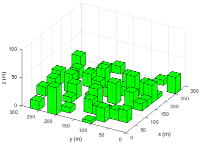
(a) A Manhattan-type city.

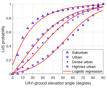
(b) Generalized logistic regression for approximating
   LoS probability.

Figure 1: Generalized logistic model for the LoS probability in a Manhattan-type city.

II-B UAV-SN Channel Model

Assuming that the complete CSI with SNs for the UAV in a given 3D space, is not known a priori, we characterize the statistical UAV-SN channel model as follows by accounting for occasional building blockage. For each SN $k$, let $c_{k,n}$ denote the binary UAV-SN channel state in each time slot $n$, where $c_{k,n}=1$ and $c_{k,n}=0$ represent respectively the LoS and NLoS states. Following the probabilistic LoS channel model [22], the uncertain channel state $c_{k,n}$ is assumed to be independently distributed over different time slots, which is practically valid when the number of time slots is sufficiently large since the actual UAV-ground CSI correlation over time can be averaged out. Moreover, in each time slot, the LoS probability, denoted by $\mathbb{P}(c_{k,n}=1)$, is a function of the UAV-SN elevation angle. Among others, one commonly used model to approximate the LoS probability is based on a simple logistic function in the form of

$$\mathbb{P}(c_{k,n}=1)=\frac{1}{1+ae^{-b(\theta_{k,n}-a)}},$$ (3)

where $\theta_{k,n}$ is the elevation angle between the UAV and SN $k$ in time slot $n$, given by

$$\theta_{k,n}=\frac{180}{\pi}\arctan\left(\frac{z_{n}}{||{\mathbf{q}}_{n}-{\mathbf{w}}_{k}||}\right),$$ (4)

and $a$ and $b$ are modeling parameters to be specified. However, this model is obtained by curve-fitting an approximate mathematical expression for the LoS probability under certain assumptions (e.g., buildings are evenly spaced between the UAV and SNs) [31] and thus may be practically inaccurate. In this paper, we improve the accuracy of the probabilistic LoS channel model by applying the combined simulation and data regression method. To be specific, we firstly simulate a Manhattan-type city as shown in Fig. 1(a) according to the typical parameters in built-up environments [31] and then compute the LoS probability under different UAV-SN elevation angles (see Appendix -A for the detailed simulation method). Next, we apply the data regression method to seek a model that can well fit the simulation data for the LoS probability versus the elevation angle in different environments. As shown in Fig. 1(b), the LoS probability, re-denoted by $P^{\rm{L}}_{k,n}\overset{\triangle}{=}\mathbb{P}(c_{k,n}=1)$ for convenience, can be largely approximated by a generalized logistic function in the following new form

$$P^{\rm{L}}_{k,n}=B_{3}+\frac{B_{4}}{1+e^{-(B_{1}+B_{2}\theta_{k,n})}},$$ (5)

where $B_{1}<0$, $B_{2}>0$, $B_{4}>0$, and $B_{3}$ are constants with $B_{3}+B_{4}=1$, which are determined by the specific environment. The corresponding NLoS probability can be obtained as $P^{\rm{N}}_{k,n}\overset{\triangle}{=}\mathbb{P}(c_{k,n}=0)=1-P^{\rm{L}}_{k,n}$. Then the large-scale channel power gain between the UAV and SN $k$ in each time slot $n$, including both the path loss and shadowing, can be approximately modeled by

$$h_{k,n}=c_{k,n}h_{k,n}^{\rm{L}}+(1-c_{k,n})h^{\rm{N}}_{k,n},$$ (6)

where

$$h_{k,n}^{\rm{L}}=\beta_{0}d_{k,n}^{-\alpha_{\rm{L}}},\leavevmode\nobreak\ \leavevmode\nobreak\ h^{\rm{N}}_{k,n}=\mu\beta_{0}d_{k,n}^{-\alpha_{\rm{N}}}$$ (7)

denote respectively the channel power gains conditioned on the LoS and NLoS states, $\beta_{0}$ is the average channel power gain at a reference distance of $d_{0}=1$ m in the LoS state, $\mu<1$ represents the additional signal attenuation factor due to the NLoS propagation, $\alpha_{\rm{L}}$ and $\alpha_{\rm{N}}$ denote respectively the average path loss exponents for the LoS and NLoS states, with $2\leq\alpha_{\rm{L}}<\alpha_{\rm{N}}\leq 6$ in practice, and

$$d_{k,n}=\sqrt{||{\mathbf{q}}_{n}-{\mathbf{w}}_{k}||^{2}+z_{n}^{2}}$$ (8)

is the distance between the UAV and SN $k$ in time slot $n$.

II-C Data Collection Model

We assume that the SNs are powered by energy harvesting and thus have sufficient energy for performing the best-effort data-transmission policy, so that they can send data to the UAV at their maximum transmit power $P_{k}$ in their scheduled transmission slots and otherwise remain in the silent mode. Let $a_{k,n}$ denote the binary communication scheduling variable for SN $k$ in time slot $n$, where SN $k$ transmits if $a_{k,n}=1$ and keeps silent otherwise. In each time slot, we assume that only one SN is scheduled for transmission, leading to the following scheduling constraints

$$\sum_{k=1}^{K}a_{k,n}\leq 1,\quad\forall n\in\mathcal{N},\qquad a_{k,n}\in\{0,1\},\quad\forall k\in\mathcal{K},n\in\mathcal{N}.$$ (9)

If SN $k$ is scheduled, the corresponding maximum achievable rate from the SN, denoted by $r_{k,n}$ in bits/second/Hertz (bps/Hz), is given by

$$r_{k,n}=\log_{2}\left(1+\dfrac{h_{k,n}P_{k}}{\sigma^{2}\Gamma}\right),$$ (10)

where $h_{k,n}$ is the real-time (large-scale) channel power gain given in (6), $\sigma^{2}$ denotes the receiver noise power, and $\Gamma>1$ is the signal-to-noise ratio (SNR) gap between the practical modulation-and-coding scheme and the theoretical Gaussian signaling. Combining (10) and (6)–(7) yields the following real-time channel-state-dependent achievable rate

$$r_{k,n}=c_{k,n}r^{\rm{L}}_{k,n}+(1-c_{k,n})r^{\rm{N}}_{k,n},$$ (11)

where

$$r^{\rm{L}}_{k,n}=\log_{2}\left(1+\dfrac{\gamma_{k}}{d_{k,n}^{\alpha_{\rm{L}}}}\right),\leavevmode\nobreak\ \leavevmode\nobreak\ r^{\rm{N}}_{k,n}=\log_{2}\left(1+\dfrac{\mu\gamma_{k}}{d_{k,n}^{\alpha_{\rm{N}}}}\right)$$ (12)

denote respectively the achievable rates conditioned on the LoS and NLoS states, and $\gamma_{k}=\frac{\beta_{0}P_{k}}{\sigma^{2}\Gamma}$.

III Problem Formulation and Proposed Hybrid Design

Consider the UAV-enabled data collection in a Manhattan-type city where the buildings are randomly and uniformly generated as described in Appendix -A. We assume that, prior to the UAV’s flight, only the knowledge of SNs’ locations and the probabilistic LoS channel model is known, while the UAV can estimate the instantaneous CSI perfectly with individual SNs in real time along its flight.

Our objective is to maximize the minimum average data collection rate from all the SNs for the UAV in one single operation. Under the constraints on the UAV trajectory and communication scheduling, the optimization problem can be formulated as follows.

$$\max_{\mathbf{Q},\mathbf{Z},\mathbf{A},\eta}\leavevmode\nobreak\ \eta$$

(P1)s.t. $$\frac{1}{N}\sum_{n=1}^{N}a_{k,n}r_{k,n}\geq\eta,\leavevmode\nobreak\ \quad\qquad\forall k\in\mathcal{K},$$ (13a)

$$||{\mathbf{q}}_{n+1}-{\mathbf{q}}_{n}||\leq S_{\rm{xy},\max},\leavevmode\nobreak\ \leavevmode\nobreak\ \quad\forall n\in\mathcal{N},$$ (13b)

$$|z_{n+1}-z_{n}|\leq S_{\rm{z},\max},\quad\qquad\forall n\in\mathcal{N},$$ (13c)

$$({\mathbf{q}}_{1}^{T},z_{1})=({\mathbf{q}}_{I}^{T},z_{I}),\leavevmode\nobreak\ \leavevmode\nobreak\ ({\mathbf{q}}_{N+1}^{T},z_{N+1})=({\mathbf{q}}_{F}^{T},z_{F}),$$ (13d)

$$H_{\min}\leq z_{n}\leq H_{\max},\leavevmode\nobreak\ \quad\qquad\forall n\in\mathcal{N},$$ (13e)

$$\sum_{k=1}^{K}a_{k,n}\leq 1,\leavevmode\nobreak\ \leavevmode\nobreak\ \leavevmode\nobreak\ \qquad\quad\qquad\forall n\in\mathcal{N},$$ (13f)

$$a_{k,n}\in\{0,1\},\leavevmode\nobreak\ \leavevmode\nobreak\ \leavevmode\nobreak\ \qquad\qquad\quad\forall k\in\mathcal{K},n\in\mathcal{N},$$ (13g)

where $\mathbf{Q}=\{\mathbf{q}_{n}\}_{n=1}^{N+1}$, $\mathbf{Z}=\{z_{n}\}_{n=1}^{N+1}$, and $\mathbf{A}=\{a_{k,n},\forall k\}_{n=1}^{N}$.

The optimal solution to problem (P1), in general, is difficult to obtain due to the lack of the complete UAV-SNs CSI at all possible UAV locations in the 3D region of interest. To address this difficulty, a key observation is that, in addition to the probabilistic LoS channel model which is known a priori, the UAV can obtain the instantaneous CSI with SNs in real time along its flight, which allows the UAV to online adjust its trajectory and communication scheduling adaptive to the random building blockage. Motivated by this, we propose in this paper a novel and general method to derive a suboptimal solution to problem (P1), called hybrid offline-online optimization, by leveraging both the statistical and real-time CSI. Our proposed method consists of the following two phases as illustrated in Fig. 2, which are briefly described as follows and will be elaborated in more details in the subsequent sections.

• Offline phase: Prior to the UAV’s flight, we design an initial UAV trajectory and communication scheduling policy based on merely the probabilistic LoS channel model. The policy is computed offline by solving an optimization problem to maximize the minimum expected rate from all the SNs. The resultant 3D UAV trajectory yields a statistically favorable UAV path that specifies the route (flying direction) the UAV follows along the trajectory, characterized by a sequence of ordered waypoints and line segments connecting them.

• Online phase: In the online phase, we fix the UAV path (waypoints) as that obtained from the offline phase. Then, at each waypoint, without changing the UAV flying direction, we formulate an LP to maximize the updated minimum expected rate from all the SNs via adjusting the UAV (horizontal and vertical) flying speeds for the remaining line segments of the offline optimized path as well as its communication scheduling with SNs over them.

Note that different from the prior joint design of UAV trajectory and communication scheduling (see e.g.,[4, 15, 14]), our proposed method decouples the design into the UAV path optimization in the offline phase, followed by the real-time adjustment of the UAV flying speeds and communication scheduling in the online phase. This is motivated by the fact that the path optimization requires solving a time-consuming non-linear optimization problem (as will be detailed in Section IV) which is desired to be implemented offline; while the online adaptation can be designed by solving an LP, which requires low computational complexity and thus can be implemented at the UAV in real time.

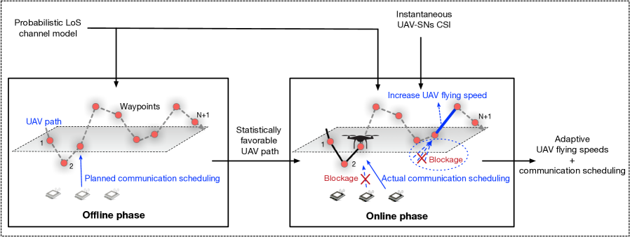
Figure 2: The proposed hybrid offline-online optimization for UAV-enabled WSNs.

Despite low real-time computational complexity, our proposed hybrid design is expected to achieve superior rate performance owing to the following reasons. First, the offline phase ensures a statistically favorable UAV path that well balances the angle-distance trade-off for maximizing the average rates with SNs over the ensemble of city realizations. Second, as compared to the offline optimized policy which may result in considerable rate loss due to the random and unknown building blockage in the actual environment, our proposed online design, built upon the offline obtained path, endows the UAV with self-adaptation to actual environment for further improving the rate performance. For instance, as illustrated in Fig. 2, if an SN scheduled for data transmission at an arbitrary line segment according to the offline policy encounters building blockage in real time, the UAV can exploit the macro-diversity to schedule another SN that happens to be in the LoS state for transmission. In a more challenging scenario, if all the SNs scheduled for transmission by the offline policy are trapped in the NLoS states in real time, the UAV can fly over this line segment at the maximum (horizontal and vertical) speeds to save time for future transmission of SNs with better channel states. On the contrary, under highly favorable channels with some SNs, the UAV can also slow down in flying to collect more data from them.

IV Proposed Offline Design

This section aims to offline design the 3D UAV trajectory and communication scheduling for maximizing the minimum expected data collection rate from all the SNs under the probabilistic LoS channel model. The computed UAV path constituting a sequence of ordered waypoints and line segments will be utilized in the online design in the next section.

IV-A Problem Transformation

In the offline phase, we focus on designing the initial 3D UAV trajectory and communication scheduling to achieve statistically favorable rate performance under the probabilistic LoS channel model. To this end, we first derive the expected rate from each SN, say SN $k$, in time slot $n$ as follows by combing (11) and (5).

$$\mathbb{E}[r_{k,n}]=P^{\rm{L}}_{k,n}r^{\rm{L}}_{k,n}+(1-P^{\rm{L}}_{k,n})r^{\rm{N}}_{k,n},\quad\forall k,n.$$ (14)

Then problem (P1) is recast as follows with the aim to maximize the minimum expected (average) rate from all the SNs, where the achievable rate $r_{k,n}$ is replaced by the expected rate $\mathbb{E}[r_{k,n}]$ given in (14).

$$\max_{\mathbf{Q},\mathbf{Z},\mathbf{A},\mathbf{\Theta},\eta}\leavevmode\nobreak\ \eta$$

(P2)s.t. $$\frac{1}{N}\sum_{n=1}^{N}a_{k,n}\mathbb{E}[r_{k,n}]\geq\eta,\quad\forall k,$$ (15a)

$$\theta_{k,n}=\frac{180}{\pi}\arctan\left(\frac{z_{n}}{||{\mathbf{q}}_{n}-{\mathbf{w}}_{k}||}\right),\leavevmode\nobreak\ \leavevmode\nobreak\ \forall k,n,$$ (15b)

$$\eqref{Eq:P1ConsStar}-\eqref{Eq:P1InterCons},$$

where $\mathbf{\Theta}=\{\theta_{k,n},\forall k\}_{n=1}^{N}$.

Problem (P2) is difficult to solve due to the non-concave rate function $\mathbb{E}[r_{k,n}]$ and the non-convex binary scheduling constraints (13g). To be specific, one can observe from (5)–(8) and (14) that $\mathbb{E}[r_{k,n}]$ is a highly complicated function of the 3D UAV trajectory, due to not only the LoS/NLoS achievable rates but also the LoS probability. It is worth mentioning that in the existing works that consider the probabilistic LoS channel model (e.g., [23, 24]), the expected rate is usually approximated by (in contrast to that given in (14))

$$\mathbb{E}[r_{k,n}]\approx\bar{r}^{\rm h}_{k,n}\triangleq\log_{2}\left(1+\dfrac{\mathbb{E}[{h}_{k,n}]P_{k}}{\sigma^{2}\Gamma}\right),$$ (16)

where $\mathbb{E}[{h}_{k,n}]=P^{\rm{L}}_{k,n}h_{k,n}^{\rm{L}}+(1-P^{\rm{L}}_{k,n})h^{\rm{N}}_{k,n}$. Such an approximation cannot guarantee the rate performance since the resultant approximate optimization problem indeed maximizes an upper bound of the expected rate due to Jensen’s inequality and the gap is non-negligible because of the significant disparity between the channel strengths under the LoS and NLoS states. To achieve more accurate approximation, an important observation is that, given the UAV’s location, the rate in the LoS state is practically much larger than that in the NLoS state due to the additional signal attenuation $\mu$ and a larger path loss exponent $\alpha_{\rm N}$ (see (7)). This implies that we can lower-bound the expected rate function in (14) as below that only accounts for the expected rate in the LoS state and thus is achievable, i.e.,

$$\!\!\!\mathbb{E}[{r_{k,n}}] \geq P^{\rm{L}}_{k,n}r^{\rm{L}}_{k,n}$$

$$=\left(B_{3}+\frac{B_{4}}{1+e^{-(B_{1}+B_{2}\theta_{k,n})}}\right)\times\log_{2}\left(1+\dfrac{\gamma_{k}}{(||{\mathbf{q}}_{n}-{\mathbf{w}}_{k}||^{2}+z_{n}^{2})^{\alpha_{\rm{L}}/2}}\right)\overset{\triangle}{=}\bar{r}^{\rm{L}}_{k,n}.$$ (17)

An illustrative example is provided as follows for demonstrating the improved accuracy and achievability of the proposed expected-rate approximation. The system parameters are given by: $\mu=20$ dB, $\alpha_{\rm L}=2.5$, $\alpha_{\rm N}=3.5$, $\beta_{0}=-60$ dB, and $\gamma_{k}=60$ dB. In time slot $n$ and for a typical user $k$ with $d_{k,n}=50$ m, the corresponding UAV-SN channel power gain conditioned on the LoS and NLoS states are obtained as $h_{k,n}^{\rm L}=-102.5$ dB and $h_{k,n}^{\rm N}=-139.5$ dB, respectively. As such, the achievable rates in the LoS and NLoS states are given by $r_{k,n}^{\rm L}=5.85$ bps/Hz and $r_{k,n}^{\rm N}=0.016$ bps/Hz, respectively. For a typical LoS probability, e.g., $P^{\rm L}_{k,n}=0.5$, the actual expected rate is $\mathbb{E}[{r_{k,n}}]=2.93$ bps/Hz. Thus, the newly-approximated expected rate, obtained as $\bar{r}_{k,n}^{\rm L}=2.92$ bps/Hz, is achievable and much more accurate than the conventionally overestimated expected rate $\bar{r}^{\rm h}_{k,n}=4.87$ bps/Hz. Based on the above expected-rate lower bound, problem (P2) can be reformulated into the following approximate form.

$$\max_{\mathbf{Q},\mathbf{Z},\mathbf{A},\mathbf{\Theta},\eta} \leavevmode\nobreak\ \eta$$

(P3)s.t. $$\frac{1}{N}\sum_{n=1}^{N}a_{k,n}\bar{r}^{\rm{L}}_{k,n}\geq\eta,\quad\forall k,$$ (18a)

$$\eqref{Eq:P1ConsStar}-\eqref{Eq:P1InterCons},\eqref{Eq:OffAngleCons}.$$

IV-B Proposed Algorithm for Problem (P3)

Problem (P3) is still challenging to solve due to the coupled horizontal and vertical trajectory variables in the non-convex rate constraints (18a) and the non-affine elevation-angle constraints (15b), as well as the integer variables in the transmission scheduling constraints (13g). To tackle these difficulties, we first relax the integer constraints for the communication scheduling, leading to the following relaxed problem

$$\max_{\mathbf{Q},\mathbf{Z},\mathbf{A},\mathbf{\Theta},\eta} \leavevmode\nobreak\ \leavevmode\nobreak\ \eta$$

(P4)s.t. $$0\leq a_{k,n}\leq 1,\quad\forall k,n,$$ (19a)

$$\eqref{Eq:P1ConsStar}-\eqref{Eq:ScheCons},\eqref{Eq:OffAngleCons},\eqref{Eq:OffMinRateCons}.$$

Then, to address the non-affine constraints (15b), we can prove by contradiction that the optimal solution to problem (P4) is the same as that to the following further relaxed problem

$$\max_{\mathbf{Q},\mathbf{Z},\mathbf{A},\mathbf{\Theta},\eta} \leavevmode\nobreak\ \leavevmode\nobreak\ \eta$$

(P5)s.t. $$\theta_{k,n}\leq\frac{180}{\pi}\arctan\left(\frac{z_{n}}{||{\mathbf{q}}_{n}-{\mathbf{w}}_{k}||}\right),\forall k,n,$$ (20a)

$$\eqref{Eq:P1ConsStar}-\eqref{Eq:ScheCons},\eqref{Eq:OffMinRateCons},\eqref{Eq:RelaxScheduling}.$$

However, problem (P5) is still non-convex for which the optimal solution is hard to obtain. As such, we propose an efficient iterative algorithm in the following based on BCD to obtain a suboptimal solution to it.

IV-B1 Communication Scheduling Optimization

Given any feasible 3D UAV trajectory $\{\mathbf{Q},\mathbf{Z}\}$, problem (P5) can be rewritten as the following problem

$$\max_{\mathbf{A},\eta}\leavevmode\nobreak\ \leavevmode\nobreak\ \eta$$

(P6)s.t. $$\eqref{Eq:ScheCons},\eqref{Eq:OffMinRateCons},\eqref{Eq:RelaxScheduling}.$$

Problem (P6) is a standard LP which can be efficiently solved by existing solvers, e.g., CVX [32]. Note that the continuous communication scheduling obtained from solving problem (P6) can be reconstructed to the binary scheduling using the method in [4] without compromising the optimality.

IV-B2 UAV Horizontal Trajectory Optimization

Given any feasible communication scheduling, $\mathbf{A}$, and UAV vertical trajectory, $\mathbf{Z}$, problem (P5) reduces to the problem below for optimizing the UAV horizontal trajectory.

$$\max_{\mathbf{Q},\mathbf{\Theta},\eta}\leavevmode\nobreak\ \leavevmode\nobreak\ \eta$$

(P7)s.t. $${\mathbf{q}}_{1}={\mathbf{q}}_{I},\quad{\mathbf{q}}_{N+1}={\mathbf{q}}_{F},$$ (22a)

$$\eqref{Eq:P1ConsStar},\eqref{Eq:OffMinRateCons},\eqref{Eq:RalxTheta}.$$

To solve this non-convex optimization problem, we first introduce an important lemma as follows.

Lemma 1.

Given $\gamma\geq 0$ and $\alpha\geq 2$, $\psi(x,y)\overset{\triangle}{=}\left(B_{3}+\frac{B_{4}}{x}\right)\log_{2}\left(1+\frac{\gamma}{y^{\alpha/2}}\right)$ is a convex function for $x>0$ and $y>0$.

Proof: See Appendix -B.  $\Box$

Using Lemma 1, we can prove that $\bar{r}^{\rm{L}}_{k,n}$ in (17) is a convex function w.r.t. $(1+e^{-{B_{1}+B_{2}\theta_{k,n}}})$ and $(||\mathbf{q}_{n}-\mathbf{w}_{k}||^{2}+z_{n}^{2})$. As such, we can apply the SCA technique to approximate the rate function $\bar{r}^{\rm{L}}_{k,n}$ by its lower bound as follows using the first-order Taylor expansion.

Lemma 2.

For any local UAV horizontal trajectory $\hat{\mathbf{Q}}$, $\bar{r}^{\rm{L}}_{k,n}$ given in (17) can be lower-bounded by

$$\bar{r}^{\rm{L}}_{k,n} \geq\hat{\bar{r}}^{\rm{L}}_{k,n}-\hat{\Omega}_{k,n}(e^{-\varphi_{k,n}}-e^{-\hat{\varphi}_{k,n}})-\hat{\Psi}_{k,n}(||\mathbf{q}_{n}-\mathbf{w}_{k}||^{2}-||\hat{\mathbf{q}}_{n}-\mathbf{w}_{k}||^{2})$$

$$\overset{\triangle}{=}\hat{\bar{r}}^{\rm{L},\rm{lb}}_{k,n},\qquad\forall k,n,$$ (23)

where $\varphi_{k,n}=B_{1}+B_{2}\theta_{k,n}$, and the coefficients $\hat{\bar{r}}^{\rm{L}}_{k,n}$, $\hat{\Omega}_{k,n}$, $\hat{\Psi}_{k,n}$ and $\hat{\varphi}_{k,n}$ are defined in Appendix -C. The equality holds at the point $\mathbf{q}_{n}=\hat{\mathbf{q}}_{n}$.

Proof: See Appendix -C.  $\Box$

For the non-convex constraints (20a), let

$$v_{k,n}\overset{\triangle}{=}\arctan\left(\frac{z_{n}}{||{\mathbf{q}}_{n}-{\mathbf{w}}_{k}||}\right).$$ (24)

One can observe that, although $v_{k,n}$ is not a concave function w.r.t. ${\mathbf{q}}_{n}$, it is a convex function w.r.t. $(||{\mathbf{q}}_{n}-{\mathbf{w}}_{k}||)$ since $\arctan(1/x)$ is convex for $x>0$. This useful property allows us to lower-bound $v_{k,n}$ as follows by using the SCA technique.

Lemma 3.

For any local UAV horizontal trajectory $\hat{\mathbf{Q}}$, $v_{k,n}$ given in (24) can be lower-bounded by

$$v_{k,n}\geq\hat{v}_{k,n}-\hat{\Lambda}_{k,n}(||{\mathbf{q}}_{n}-{\mathbf{w}}_{k}||-||{\hat{\mathbf{q}}}_{n}-{\mathbf{w}}_{k}||)\overset{\triangle}{=}\hat{v}^{\rm{lb}}_{k,n},\qquad\forall k,n,$$ (25)

where the coefficients $\hat{v}_{k,n}$ and $\hat{\Lambda}_{k,n}$ are respectively given by

$$\hat{v}_{k,n}=\arctan\left(\frac{z_{n}}{||{\hat{\mathbf{q}}}_{n}-{\mathbf{w}}_{k}||}\right),\leavevmode\nobreak\ \leavevmode\nobreak\ \leavevmode\nobreak\ \hat{\Lambda}_{k,n}=\frac{z_{n}}{||{\hat{\mathbf{q}}}_{n}-{\mathbf{w}}_{k}||^{2}+z_{n}^{2}}.$$ (26)

The equality holds at the point $\mathbf{q}_{n}=\hat{\mathbf{q}}_{n}$.

Using Lemmas 2 and 3, problem (P7) can be reformulated into the approximate form given below, where $\bar{r}^{\rm{L}}_{k,n}$ in (18a) and $v_{k,n}$ in (20a) are replaced by their corresponding lower bounds.

$$\max_{\mathbf{Q},\mathbf{\Phi},\mathbf{\Theta},\eta}\leavevmode\nobreak\ \eta$$

(P8)s.t. $$\frac{1}{N}\sum_{n=1}^{N}a_{k,n}\hat{\bar{r}}^{\rm{L},\rm{lb}}_{k,n}\geq\eta,\qquad\forall k,$$ (27a)

$$\varphi_{k,n}=B_{1}+B_{2}\theta_{k,n},\qquad\forall k,n,$$ (27b)

$$\theta_{k,n}\leq\frac{180}{\pi}\hat{v}^{\rm{lb}}_{k,n},\qquad\qquad\forall k,n,$$ (27c)

$$\eqref{Eq:P1ConsStar},\eqref{Eq:P8StarEnd},$$

where $\mathbf{\Phi}=\{\varphi_{k,n},\forall k\}_{n=1}^{N}$. The approximate problem (P8) is a convex optimization problem and thus can be efficiently solved by using existing solvers, e.g., CVX. It is worth mentioning that, by approximating the non-convex constraints with their convex lower bounds, the feasible set of problem (P8) is always a subset of problem (P7). This guarantees that solving problem (P8) gives a lower bound of the optimal objective value of problem (P7).

IV-B3 UAV Vertical Trajectory Optimization

Last, given any feasible communication scheduling, $\mathbf{A}$, and UAV horizontal trajectory, $\mathbf{Q}$, problem (P5) reduces to the following problem for optimizing the UAV vertical trajectory.

$$\max_{\mathbf{Z},\mathbf{\Theta},\eta}\leavevmode\nobreak\ \leavevmode\nobreak\ \leavevmode\nobreak\ \eta$$

(P9)s.t. $$z_{1}=z_{I},\leavevmode\nobreak\ \leavevmode\nobreak\ \leavevmode\nobreak\ z_{N+1}=z_{F},$$ (28a)

$$\eqref{Eq:P1VerSpeed},\eqref{Eq:zmin},\eqref{Eq:OffMinRateCons},\eqref{Eq:RalxTheta}.$$

Since problem (P9) has a similar form as problem (P7), we can apply a similar approach as for solving problem (P7) (i.e., applying the SCA technique to the constraints (18a)) and thereby problem (P9) can be transformed to the following problem

$$\max_{\mathbf{Z},\mathbf{\Phi},\mathbf{\Theta},\eta}\leavevmode\nobreak\ \leavevmode\nobreak\ \eta$$

(P10)s.t. $$\frac{1}{N}\sum_{n=1}^{N}a_{k,n}\check{\bar{r}}^{\rm{L},\rm{lb}}_{k,n}\geq\eta,\forall k,$$ (29a)

$$\eqref{Eq:P1VerSpeed},\eqref{Eq:zmin},\eqref{Eq:RalxTheta},\eqref{Eq:utheta},\eqref{Eq:P11z},$$

where $\check{\bar{r}}^{\rm{L},\rm{lb}}_{k,n}$ is the lower bound of $\bar{r}^{\rm{L}}_{k,n}$ given a local vertical trajectory $\check{\mathbf{Z}}$, which can be obtained by using a similar SCA technique as in Lemma 2. Note that in (20a), $v_{k,n}$ is a convex function w.r.t. $z_{n}$, since $\arctan(x)$ is a concave function for $x>0$. Thus, problem (P10) is a convex optimization problem, which can be optimally solved by using the interior-point method in general. In practice, due to the lack of support for the function of $\arctan(x)$ in CVX, we can approximate $\arctan(x)$ by its upper bound using the first-order Taylor expansion for simplicity.

IV-B4 Overall Algorithm and Computational Complexity

Using the results in the preceding subsections, an iterative algorithm can be proposed to obtain a suboptimal solution to problem (P3) by alternately optimizing the transmission scheduling of SNs, UAV horizontal and vertical trajectories. In addition, the initial UAV trajectory can be constructed as the straight flight from the initial location to the final location. Next, we discuss the computational complexity of the proposed algorithm. Since the communication scheduling, and UAV horizontal and vertical trajectories are sequentially optimized in each iteration by using the CVX solver which is based on the standard interior-point method, their individual complexities scale as $\mathcal{O}((KN)^{3.5}\log(1/\epsilon))$, $\mathcal{O}((N+KN)^{3.5}\log(1/\epsilon))$, and $\mathcal{O}((N+KN)^{3.5}\log(1/\epsilon))$, respectively, given a solution accuracy of $\epsilon>0$ [33]. Then accounting for the BCD iterations with the complexity of $\log(1/\epsilon)$, the total computational complexity of the algorithm is thus $\mathcal{O}((N+KN)^{3.5}\log^{2}(1/\epsilon))$, which is affordable for offline computation. Moreover, the algorithm is shown to always converge in our extensive simulations (see Section VI-A). Last, the UAV path obtained from the offline phase is represented by the waypoints $\{({\mathbf{q}}_{n}^{T*},z^{*}_{n})\}_{n=1}^{N+1}$, which denote a suboptimal solution to problem (P3) computed by the iterative algorithm.

V Proposed Online Design

Directly implementing the offline optimized UAV trajectory and communication scheduling policy in practice may suffer considerable rate loss due to the lack of online adaptation to the random building blockage. This issue is addressed in this section by designing the online policy that adaptively adjusts the UAV flying speeds along the offline optimized UAV path as well as its communication scheduling with SNs based on the real-time UAV-SNs CSI and SNs’ individual amounts of data received accumulatively.

To this end, the UAV path (instead of time) is discretized into $N$ line segments with the $(N+1)$ waypoints fixed as those obtained from the offline phase, i.e., $\{({\mathbf{q}}_{n}^{T*},z^{*}_{n})\}_{n=1}^{N+1}$ [24]. At each line segment, the distance between the UAV and each SN can be assumed to be approximately unchanged due to the time discretization method adopted in the offline phase. Unless otherwise stated, we reuse the notations w.r.t. the time slot under time discretization for the current case w.r.t. the line segment for convenience. In the online phase, we assume that the UAV flies at a constant speed over each line segment horizontally as well as vertically. To enforce that the UAV follows the offline optimized path, the time durations spent on traveling the horizontal and vertical distances at each line segment $n$ need to be identical and thus commonly denoted by $t_{n},\forall n$. Then the UAV flying velocity at each line segment is given by

$$\mathbf{v}_{n}=\frac{\left(\mathbf{q}^{T*}_{n+1}-\mathbf{q}^{T*}_{n},z^{*}_{n+1}-z^{*}_{n}\right)^{T}}{t_{n}},\quad\forall n\in\mathcal{N},$$ (30)

and the corresponding horizontal and vertical flying speeds are respectively given by

$$v_{{\rm{xy}},n}=\frac{||\mathbf{q}^{*}_{n+1}-\mathbf{q}^{*}_{n}||}{t_{n}},\leavevmode\nobreak\ \leavevmode\nobreak\ \leavevmode\nobreak\ v_{{\rm{z}},n}=\frac{|z^{*}_{n+1}-z^{*}_{n}|}{t_{n}},\quad\forall n\in\mathcal{N}.$$ (31)

As a result, the optimization of the UAV flying speeds at each line segment can be equivalently transformed to that of the traveling duration. For the proposed online policy, let $T^{\rm{re}}_{n}$ denote the remaining flight duration from the beginning of each line segment $n$, which evolves as

$$T^{\rm{re}}_{1}=T_{0},\leavevmode\nobreak\ \leavevmode\nobreak\ T^{\rm{re}}_{n}=T^{\rm{re}}_{n-1}-t_{n-1},n>1.$$ (32)

Moreover, instead of using the communication scheduling $a_{k,n}$ obtained in the offline phase, we define $\tau_{k,n}\geq 0$ as the allocated data-transmission time for SN $k$ at line segment $n$. Then the amount of received data (in bits/Hz) at the UAV from SN $k$ over the $n$-th line segment is given by $\tau_{k,n}r_{k,n}$ and the amount of accumulatively received data up to the beginning of each line segment $n$, denoted by $r^{\rm{ac}}_{k,n}$, evolves as

$$r^{\rm{ac}}_{k,1}=0,\leavevmode\nobreak\ \leavevmode\nobreak\ \leavevmode\nobreak\ r^{\rm{ac}}_{k,n}=\sum_{m=1}^{n-1}\tau_{k,m}r_{k,m},\leavevmode\nobreak\ \leavevmode\nobreak\ n>1,\forall k\in\mathcal{K}.$$ (33)

To formulate the optimization problem in the online phase, since the UAV re-optimizes its policy at each waypoint $n$ including its traveling durations and communication durations with SNs over all the subsequent line segments $m=n,\cdots,N$, we re-denote $\tau_{k,m}$ and $t_{k,m}$ by $\tau_{k,m}^{(n)}$ and $t_{m}^{(n)}$ as the variables in the $n$-th policy optimization. The online policy needs to satisfy the following constraints. First, the finite UAV horizontal and vertical flying speeds enforce that

$$v_{{\rm{xy}},m}\leq V_{\rm{xy},\max},\leavevmode\nobreak\ \leavevmode\nobreak\ v_{{\rm{z}},m}\leq V_{\rm{z},\max},\quad m=n,\cdots,N.$$ (34)

Combining (34) and (31) yields

$$t_{m}^{(n)}\geq\max\left\{\frac{||\mathbf{q}^{*}_{m+1}-\mathbf{q}^{*}_{m}||}{V_{\rm{xy},\max}},\frac{|z^{*}_{m+1}-z^{*}_{m}|}{V_{\rm{z},\max}}\right\}\overset{\triangle}{=}\hat{t}_{m},\quad m=n,\cdots,N.$$ (35)

Second, the total traveling duration over the remaining line segments should satisfy $\sum_{m=n}^{N}t_{m}^{(n)}\leq T^{\rm{re}}_{n}$. Last, the communication scheduling constraint in (13f) is re-written by

$$\sum_{k=1}^{K}\tau_{k,m}^{(n)}\leq t_{m}^{(n)},\quad m=n,\cdots,N.$$ (36)

For the rate performance, let $r_{k,n}^{\rm{ave}}$ denote the updated expected average rate from SN $k$ at waypoint $n$, which is given by

$$r_{k,n}^{\rm{ave}}=\frac{1}{T_{0}}\left(r^{\rm{ac}}_{k,n}+\tau_{k,n}^{(n)}r_{k,n}+\sum_{m=n+1}^{N}\tau_{k,m}^{(n)}\mathbb{E}[r_{k,m}]\right),\leavevmode\nobreak\ \leavevmode\nobreak\ \forall k\in\mathcal{K},$$ (37)

accounting for the amounts of data received accumulatively, $r^{\rm{ac}}_{k,n}$, achieved in the current line segment, $\tau_{k,n}^{(n)}r_{k,n}$, and expected to be received over subsequent line segments, $\sum_{m=n+1}^{N}\tau_{k,m}^{(n)}\mathbb{E}[r_{k,m}]$. Note that in (37), $r_{k,n}$ is determined by the instantaneous CSI (see (11)) and $\{\mathbb{E}[r_{k,m}],\forall k\}_{m=n+1}^{N}$ can be explicitly obtained from (14) with the LoS probabilities determined by the fixed waypoints according to (4)–(5). Based on the above discussion, the optimization problem for the online adaptation at each waypoint can be modified from that for the offline design, i.e., problem (P2), as formulated below.

$$\max_{\bm{\tau}^{(n)},\mathbf{T}^{(n)},\eta^{(n)}}\leavevmode\nobreak\ \leavevmode\nobreak\ \eta^{(n)}$$

(P11)s.t. $$r_{k,n}^{\rm{ave}}\geq\eta^{(n)},\quad\forall k\in\mathcal{K},$$ (38a)

$$\tau_{k,m}^{(n)}\geq 0,\quad\quad\forall k\in\mathcal{K},m=n,\cdots,N,$$ (38b)

$$\eqref{Eq:OnlineEachT}-\eqref{Eq:OnlineTimeShare},$$

where $\bm{\tau}^{(n)}=\{\tau_{k,m}^{(n)},\forall k\}_{m=n}^{N}$ and $\mathbf{T}^{(n)}=\{t_{m}^{(n)}\}_{m=n}^{N}$.

Problem (P11) is a standard LP and thus can be efficiently solved by existing solvers, e.g., CVX. Let $\{\tau_{k,n}^{(n)*},\forall k\}_{m=n}^{N}$, $\{t^{(n)*}_{m}\}_{m=n}^{N}$, and $\eta^{(n)*}$ denote the optimal solution to problem (P11). By using contradiction, we can easily show that the UAV tends to schedule SNs for data transmission at the line segments with relatively high instantaneous achievable rate $r_{k,n}$ or the expected rate $\mathbb{E}[r_{k,m}]$, while at the same time, balancing with the SNs’ individual average rates. This observation indicates that the online policy allows the UAV to adaptively schedule data transmissions from the SNs with high real-time achievable rates by exploiting the channel macro-diversity. Moreover, for the line segment where most of the SNs are in the NLoS states with relatively low achievable rates, the UAV is expected to reduce the traveling duration over it to save time for future transmission of SNs with better channel states.

It is worth mentioning that, at each waypoint $n$, the computational complexity for solving problem (P11) using the interior method scales as $\mathcal{O}\left(((K+1)(N-n+1))^{3.5}\right)$, which decreases along the UAV path due to the decreasing number of the optimization variables associated with the remaining line segments. In practice, solving an LP takes relatively short running time as will be demonstrated in Section VI-B. Last, combining the analysis for the convergence and complexity of the offline design in Section IV-B4, the proposed hybrid offline-online optimization method can be shown to always converge to a suboptimal solution of problem (P1) and has an overall complexity order of $\mathcal{O}\left(((K+1)(N-n+1))^{3.5}+(N+KN)^{3.5}\log^{2}(1/\epsilon)\right)$.

Remark 1 (Practical implementation).

Prior to the UAV’s flight, the initial joint design of UAV trajectory and communication scheduling is offline computed by the iterative algorithm in Section IV-B4. The information of the optimized waypoints, $\{({\mathbf{q}}_{n}^{T*},z^{*}_{n})\}_{n=1}^{N+1}$, is stored at the UAV, based on which the UAV can compute the expected rates from individual SNs at each line segment, $\{\mathbb{E}[r_{k,n}],\forall k\}_{n=1}^{N}$. During the UAV’s flight, at each waypoint $n$, the UAV first acquires the instantaneous CSI with SNs $\{c_{k,n},\forall k\}$ and then computes the optimal solution to problem (P11) with the updated information of $\{r^{\rm{ac}}_{k,n},\forall k\}$ and $T^{\rm{re}}_{n}$. Last, the UAV applies the communication scheduling for the current line segment $n$ according to $\{\tau_{k,n}^{(n)*},\forall k\}$, and at the same time, heads towards the next waypoint at the horizontal and vertical speeds determined by $t^{(n)*}_{n}$ and (31).

Remark 2 (DoF for online speed optimization).

The total flight duration $T_{0}$ affects the DoF for speed optimization in the online phase. Specifically, given a relatively short flight duration, the UAV designed in the offline phase tends to sequentially visit each SN as close as possible at the maximum horizontal speed. As observed from (35), this will limit the DoF for speed optimization in the online phase even with a large maximum vertical speed. In contrast, with a relatively long flight duration, the UAV can more flexibly accelerate or slow down in its real-time flight as long as it can reach the final location in time.

Remark 3 (Proposed method versus open-loop feedback control).

The proposed online adaptation partially resembles the celebrated open-loop feedback control (OLFC) [34] that computes an open-loop policy at the current time as if no future (channel) state information will be available. However, when applying to our considered problem, OLFC requires solving a joint optimization problem for the UAV trajectory and communication scheduling in each time slot using an algorithm similar to the iterative algorithm in Section IV-B4 with sequentially reduced dimension, whose computational complexity may be too high to be implementable at the UAV in real time. In contrast, our proposed hybrid design solves the time-consuming path optimization problem in the offline phase, and only refines a simplified open-loop policy in the online phase for adjusting the UAV flying speeds and communication scheduling by solving a low-complexity LP, thus making it amenable to real-time implementation by the UAV.

Remark 4 (Extension to the energy-constrained SNs).

The results of this paper for the renewable energy-powewed SNs can be extended to the energy-constrained SNs as follows. First, let $P_{k,n}$ denote the transmit power of SN $k$ in time slot $n$, which needs to satisfy the long-term power constraint: $\frac{1}{N}\sum_{n=1}^{N}P_{k,n}\leq P_{k,\max},\forall k$, where $P_{k,\max}$ is the maximum average transmit power of SN $k$. Then the approximated expected rate, $\bar{r}^{\rm{L}}_{k,n}$ in (17), can be re-expressed as $\bar{r}^{\rm{L}}_{k,n}\triangleq\left(B_{3}+\frac{B_{4}}{1+e^{-(B_{1}+B_{2}\theta_{k,n})}}\right)\times\log_{2}\left(1+\dfrac{P_{k,n}\gamma_{0}}{a_{k,n}(||{\mathbf{q}}_{n}-{\mathbf{w}}_{k}||^{2}+z_{n}^{2})^{\alpha_{\rm{L}}/2}}\right)$. As such, the offline design can be modified by reformulating the communication-scheduling problem (P3) as the joint optimization problem for the communication scheduling and SNs’ transmit power allocation, which can be shown to be a convex optimization problem. Similarly, the online design can be modified by reformulating the optimization problem (P11) as the joint optimization problem for the UAV’s flying speeds as well as SNs’ transmit power allocation, without changing the main solution approach proposed in this paper.

VI Simulation Results

In this section, we provide extensive simulation results to verify the effectiveness of the proposed hybrid offline-online design and show key properties of the optimized 3D offline and online UAV trajectories as well as the adaptive communication scheduling. Unless otherwise stated, the following results are based on a random realization of $4$ SNs’ locations over a square area of $300\times 300$ $\rm{m}^{2}$ for ease of illustration. The UAV is assumed to fly from an initial location $(0,150,50)$ m to a final location $(300,150,50)$ m. Assume that all the SNs have the same transmit power of $0.1$ W. We consider an urban environment for which the parameters of its corresponding generalized logistic model for the LoS probability are given by $B_{1}=-0.4568$, $B_{2}=0.0470$, $B_{3}=-0.63$, and $B_{4}=1.63$. Other parameters are set as $\beta_{0}=-60$ dB, $\Gamma=8.2$ dB, $\sigma^{2}=-109$ dBm, $\alpha_{\rm{L}}=2.5$, $\alpha_{\rm{N}}=3.5$, $\mu=-20$ dB, $V_{\rm{xy},\max}=40$ m/s, $V_{\rm{z},\max}=20$ m/s, $H_{\min}=50$ m, $H_{\max}=300$ m, $\delta=0.2$ s, and $\epsilon=0.001$.

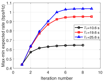
Figure 3: Max-min expected rate versus iteration number.

VI-A Offline Phase

We first evaluate the performance of the proposed initial 3D UAV trajectory design in the offline phase. To start with, we first show the convergence behavior of the iterative algorithm in Section IV-B4 under different flight durations in Fig. 3. It can be observed that the max-min expected rate based on the probabilistic LoS channel model monotonically increases with the number of iterations and quickly converges after around $10$ iterations for all flight durations.

For performance comparison, we consider two benchmark schemes: 1) LoS-based (LB) scheme, which jointly designs UAV trajectory and communication scheduling based on the simplified LoS channel model (i.e., assuming the LoS probability given in (5) to be $P^{\rm{L}}_{k,n}=1,\forall k,n$); 2) probabilistic-LoS with the lowest altitude (PLLA) that only optimizes the UAV horizontal trajectory and communication scheduling with the UAV altitude kept equal to $H_{\min}$ for all time. Our proposed scheme is named as probabilistic-LoS based (PLB) scheme for convenience. Fig. 4 illustrates the UAV trajectories by different schemes with the flight duration $T_{0}=10.6$ s. Several interesting observations are made as follows. First, as shown in Fig. 4(a), the three schemes have similar horizontal trajectories with the UAV sequentially traveling around each SN, but differ in that, the UAV for both the PLB and PLLA schemes moves closer to SNs $1$ and $2$ than that of the LB scheme when traveling nearby them, at the cost of being more away from SN $4$. The reason is that the elevation angles of the UAV with SNs $1$ and $2$ are relatively small and thus need to be enlarged by tuning the UAV horizontal trajectory, which is not seen in the trajectory by the LB scheme. Second, for the 3D UAV trajectory shown in Fig. 4(b), we can observe that the proposed PLB scheme can exploit the additional DoF brought by the UAV vertical trajectory to balance the angle-distance trade-off more efficiently than the PLA scheme as the elevation angle can be effectively enlarged by moderately increasing the altitude without incurring significant path loss.

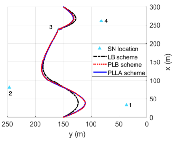
(a) UAV horizontal trajectory.

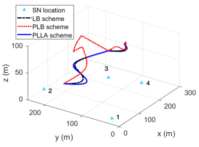
(b) 3D UAV trajectory.

Figure 4: Comparison of the UAV trajectories by different schemes with $T_{0}=10.6$ s.

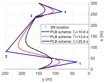
(a) UAV horizontal trajectory.

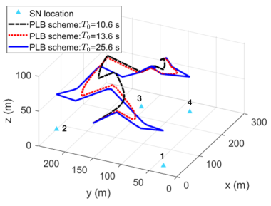
(b) 3D UAV trajectory.

Figure 5: Comparison of the UAV trajectories by the PLB scheme under different UAV flight durations.

In Fig. 5, we compare the UAV trajectories by the proposed PLB scheme under different UAV flight durations. It is observed that given a short flight duration (e.g., $T_{0}=10.6$ s), the UAV flies at a relatively high altitude to maintain appropriate elevation angles with SNs for increasing the LoS probabilities. As the flight duration increases, the UAV lowers its altitude and moves closer to the SNs when traveling around them. Specifically, with a sufficiently long flight duration (e.g., $T_{0}=25.6$ s), the UAV can sequentially hover right above each SN at the minimum altitude for a certain amount of time, which is expected since by this way, the UAV can attain the largest elevation angle with each SN, and at the same time, experience the minimum path loss.

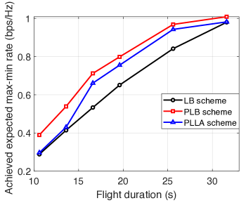
Figure 6: Offline phase: achieved expected max-min rate versus flight duration.

Fig. 6 plots the curves of the achieved expected max-min rates by different offline schemes averaged over $100$ city realizations versus the UAV flight duration. Note that there is no online adjustment of UAV flying speeds and communication scheduling here. We can observe that the PLLA scheme achieves larger rates than the LB scheme, since it optimizes the UAV horizontal trajectory based on the more accurate probabilistic LoS channel model instead of the simplified LoS channel model. In addition, the proposed PLB scheme can further improve the rate performance as compared to the PLLA scheme, since it exploits the UAV vertical trajectory to further reduce the blockage effect. However, the rate performance gain diminishes as the UAV flight duration increases, which is expected since all the schemes have similar trajectories when the flight duration is sufficiently long, i.e., the UAV will spend more time on hovering above SNs at its lowest altitude to achieve the highest rates with them, while the time and achieved rates when it is flying become less significant.

VI-B Online Phase

Next, we study the effectiveness of the proposed online design by fixing the UAV path as that obtained from the offline phase by the PLB scheme. For performance comparison, we consider the following online schemes: 1) PLB scheme without any online adjustment; 2) adaptive communication scheduling (ACS) that only online updates the communication scheduling by solving an LP in each time slot which has a similar form as problem (P11), but without the optimization of UAV flying speeds; 3) our proposed scheme with joint communication scheduling and UAV flying speed adaptation, thus named as joint adaptation (JA); and 4) optimal joint adaptation (OJA) assuming the ideal case of perfect (non-causal) UAV-SNs CSI along the offline obtained UAV path, which jointly optimizes UAV flying speeds and communication scheduling by solving a similar problem as problem (P11) with the expected rate replaced by the exact rate.

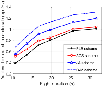
(a) Online phase: achieved expected max-min rate
   versus flight duration.

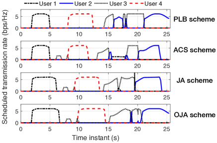
(b) Scheduled transmission rate.

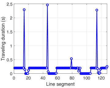
(c) Traveling durations of the JA scheme.

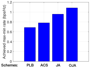
(d) Achieved max-min rate.

Figure 7: (a): Comparison of the rate performance by different online schemes versus flight duration; (b)-(d): rate performance and traveling durations of different online schemes in a random city realization with $T_{0}=25.6$ s.

In Fig. 7(a), we compare the achieved expected max-min rates by different online schemes over $100$ city realizations versus the flight duration. First, it is observed that, for all schemes, the expected max-min rate first increases with the flight duration and then tends to saturate in the regime of long flight duration due to the similar reason given for the offline case (see Fig. 6). Second, although the simple ACS scheme outperforms the PLB scheme, its performance gain diminishes with the flight duration. The reason is that, with a sufficiently long flight duration, the dominant rate is contributed by the regime where the UAV flies (nearly) above each SN and thus the UAV has a high likelihood to establish an LoS link with the SN underneath, which renders the online communication-scheduling adaptation less effective. This limitation, however, can be alleviated by the proposed JA scheme, which further adjusts the UAV flying speeds in real time along the path such that it can spend more time on the line segments that contribute to relatively higher achievable rates, thus sustaining the rate gain even for the case of long flight duration. Last, it is worth noting that OJA scheme achieves the highest max-min rates since it has full and non-causal CSI along the UAV path, thus providing a performance upper bound for our proposed JA scheme with causal CSI only.

To further illustrate the proposed JA scheme for the online phase, we compare the rate performance in a random city realization with $T_{0}=25.6$ s. One can observe from Fig. 7(b) that the achieved rate from SN $1$ is the performance bottleneck of the PLB scheme. The ACS scheme can slightly improve the average rate of SN $1$ by scheduling it for transmission in idle time slots without significantly compromising the rates of other SNs. In contrast, our proposed JA scheme can further improve the max-min rate over the ACS scheme as shown in Fig 7(d) by online adjusting the traveling duration at each line segment based on the instantaneous CSI with SNs (see Fig. 7(c)). Again, the OJA scheme can make full use of the non-causal CSI to improve the average rates from all SNs, thus achieving the largest max-min rate.

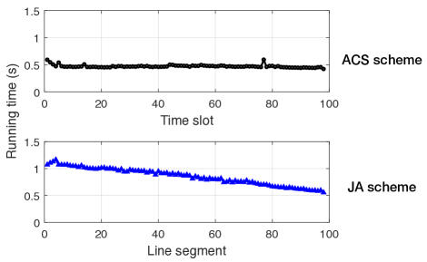
(a) Running time of two online schemes in a random city
  realization with $T_{0}=19.6$ s.

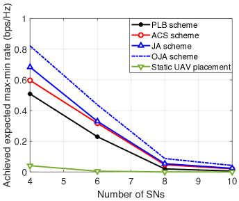
(b) Achieved max-min rate versus number of SNs.

Figure 8: (a): Running time of two online schemes; (b): effects of the number of SNs.

To demonstrate the required computational complexity for implementing the proposed online designs, we compare the running time of the ACS and JA schemes using Matlab on a computer equipped with Intel Core i5-7500, 3.40 GHz processor, and 8 GB RAM memory. Fig. 8(a) shows the running time of the two schemes for a random city realization with $T_{0}=19.6$ s. It is observed that the proposed JA scheme takes slightly longer running time than the ACS scheme due to the joint online optimization of UAV flying speeds and communication scheduling for achieving larger max-min rates (see Fig. 7(a)). Moreover, the running time of the proposed JA scheme decreases along the UAV path or the increasing line-segment index, which is expected since the required number of optimization variables reduces as the UAV flies to the destination. Overall, the required computation time over each line segment is in the order of a second for both online schemes, which is practically affordable.

Last, we compare in Fig. 8(b) the achieved expected max-min rates by different online schemes versus the number of SNs. To show the gain of trajectory optimization, we consider another benchmark scheme called static UAV placement, for which the UAV’s horizontal placement is determined by the K-means clustering algorithm based on SNs’ locations, the altitude is optimized by using a similar algorithm as for optimizing the vertical trajectory in this paper, and the communication scheduling is optimized according to the actual UAV-SNs channel states. It is observed that the expected max-min rates of all schemes decrease with the number of SNs, since more SNs share the communication resource and the max-min rate is restricted by the worst-case SN that achieves the lowest rate. Moreover, all the schemes that deploy a flying UAV for data collection significantly outperforms the benchmark with a static UAV. The reason is that the achieved max-min rate by deploying a static UAV is severely affected by the UAV-SNs channel states at the optimized UAV’s location and can be extremely low if one of the SNs is in the NLoS state, whereas deploying a flying UAV can resolve this issue by exploiting the time-varying channel states with SNs.

VII Conclusions

This paper studies the UAV-enabled WSN by deploying a UAV to collect data from distributed SNs in a Manhattan-type city, for which a new probabilistic LoS channel model is constructed and shown in the form of a generalized logistic function of the UAV-SN elevation angle. We consider that the UAV only has the knowledge of SNs’ locations and the probabilistic LoS channel model of the environment prior to its flight, while it can obtain obtain the instantaneous UAV-SNs CSI along its flight. Our objective is to maximize the minimum (average) data collection rate from all the SNs for the UAV. To this end, we first formulate a rate maximization problem by jointly optimizing the 3D UAV trajectory and communication scheduling. Then we propose a novel design method, called hybrid offline-online optimization, to obtain a suboptimal solution to it, by leveraging both the statistical and real-time CSI. Our proposed method decouples the joint design of UAV trajectory and communication scheduling into two phases: namely, an offline phase that determines the UAV path based on the probabilistic LoS channel model, followed by an online phase that jointly adjusts the UAV flying speeds and communication scheduling along the offline optimized UAV path based on the instantaneous UAV-SNs CSI and SNs’ individual amounts of data received accumulatively. Simulation results demonstrate the effectiveness of the proposed hybrid design and reveal key insights into the joint offline-online 3D UAV trajectory and communication scheduling optimization.

The proposed hybrid design for UAV-enabled WSNs opens many interesting and important directions that deserve further in-depth investigation, some of which as discussed as follows. First, besides the adopted probabilistic LoS channel model, there exist many other stochastic UAV-ground channel models in the literature, such as the nested segmented ray-tracing channel model and the 3D geometry-based stochastic channel model [2]. Therefore, it is worth studying whether/how we can apply/extend the proposed hybrid design method to optimize the UAV trajectory and communication scheduling under these channel models. Next, considering the ideal case where the complete UAV-SNs CSI is known a priori, the corresponding optimal solution to our studied problem will provide a performance upper bound for our proposed hybrid design with statistical and partial CSI only. However, how to obtain the optimal solution efficiently is still an open problem and thus needs further investigation. In addition, it is interesting to extend the current work assuming one single data collection operation to the scenario with multiple operations. This setting introduces new design challenges, for example, how to make use of the limited CSI obtained from the previous operations to design the UAV trajectory in the subsequent operations for improving their rate performance. Last, in practice, to further enhance the system rate performance, multiple UAVs can be deployed to collect data from SNs. In this scenario, it is critical to design the cooperation schemes among the UAVs in both the offline and online phases by leveraging the shared CSI for achieving different objectives such as the maximum min-rate and the maximum energy efficiency.

-A Simulation-Based Modeling for LoS Probability

Consider a Manhattan-type city where the whole area is partitioned into uniform square grids in the average size of buildings therein which can be obtained based on typical city parameters [31]. We first randomly and uniformly generate the buildings in the square grids with random heights following the Rayleigh distribution (see Fig. 1(a)). Next, a set of SNs are randomly generated on the area unoccupied by the buildings. By using a similar simulation method as in [35], we then obtain the LoS/NLoS channel states under different UAV-SN elevation angles. Specifically, to account for the effect of UAV horizontal location on the LoS probability, we fix the UAV altitude and change the UAV horizontal location according to the elevation angle (from $5^{\circ}$ to $90^{\circ}$ with a step size of $5^{\circ}$), whereas the azimuth angle ranges from $0^{\circ}$ to $360^{\circ}$ with a step size of $30^{\circ}$ for each elevation angle. We repeat this procedure for different UAV altitudes ranging from $30$ m to $300$ m with a step size of $30$ m for characterizing the effect of UAV altitude on the LoS probability. Last, the LoS probability is calculated based on the obtained LoS/NLoS states over $200$ randomly-generated cities for each type of environment (see Fig. 1(b)).

-B Proof of Lemma 1

Define $\xi(x,y)\overset{\triangle}{=}\left(B_{3}+\frac{B_{4}}{x}\right)\ln\left(1+\frac{\gamma}{y^{\alpha/2}}\right)$. We first prove the convexity of $\xi(x,y)$ by the definition of convex functions. To this end, we first derive that first-order derivatives of $\xi(x,y)$ w.r.t. $x$ and $y$, as follows.

$$\xi_{x}(x,y)=-\frac{B_{4}}{x^{2}}\ln\left(1+\frac{\gamma}{y^{\alpha/2}}\right),\quad\xi_{y}(x,y)=-\left(B_{3}+\frac{B_{4}}{x}\right)\frac{\gamma\alpha/2}{y(y^{\alpha/2}+\gamma)}.$$ (39)

Then, the Hessian of $\xi(x,y)$ is

$$\bigtriangledown^{2}\xi(x,y)=\left[\begin{array}[]{cc}\dfrac{2B_{4}}{x^{3}}\ln\left(1+\dfrac{\gamma}{y^{\alpha/2}}\right)&\dfrac{B_{4}\gamma\alpha/2}{x^{2}y(y^{\alpha/2}+\gamma)}\\ \dfrac{B_{4}\gamma\alpha/2}{x^{2}y(y^{\alpha/2}+\gamma)}&\left(B_{3}+\dfrac{B_{4}}{x}\right)\dfrac{\gamma\alpha/2[(\alpha/2+1)y^{\alpha/2}+\gamma]}{y^{2}(y^{\alpha/2}+\gamma)^{2}}\end{array}\right].$$ (40)

Given $\alpha\geq 2$, for any $\mathbf{t}=[t_{1},t_{2}]^{T}$, we have

$$\mathbf{t}^{T}\bigtriangledown^{2}\xi(x,y)\mathbf{t}$$

$$= t_{1}^{2}\left(\frac{2B_{4}}{x^{3}}\ln\left(1+\frac{\gamma}{y^{\alpha/2}}\right)\right)+t_{2}^{2}\left(\left(B_{3}+\frac{B_{4}}{x}\right)\frac{\gamma\alpha/2[(\alpha/2+1)y^{\alpha/2}+\gamma]}{y^{2}(y^{\alpha/2}+\gamma)^{2}}\right)+2t_{1}t_{2}\left(\frac{B_{4}\gamma\alpha/2}{x^{2}y(y^{\alpha/2}+\gamma)}\right)$$

$$\overset{(i)}{\geq} t_{1}^{2}\left(\frac{2B_{4}}{x^{3}}\frac{\gamma}{y^{\alpha/2}+\gamma}\right)+t_{2}^{2}\left(\left(B_{3}+\frac{B_{4}}{x}\right)\frac{\gamma(2y^{\alpha/2}+\gamma)}{y^{2}(y^{\alpha/2}+\gamma)^{2}}\right)+2t_{1}t_{2}\left(\frac{B_{4}\gamma}{x^{2}y(y^{\alpha/2}+\gamma)}\right)$$

$$= \frac{2t_{1}^{2}B_{4}\gamma y^{2}(y^{\alpha/2}+\gamma)+t_{2}^{2}\gamma x^{3}(B_{3}+\frac{B_{4}}{x})(2y^{\alpha/2}+\gamma)+2t_{1}t_{2}B_{4}\gamma xy(y^{\alpha/2}+\gamma)}{x^{3}y^{2}(y^{\alpha/2}+\gamma)^{2}}$$

$$= \frac{\gamma[(y^{\alpha/2}+\gamma)B_{4}(t_{1}y+t_{2}x)^{2}+(y^{\alpha/2}+\gamma)(B_{4}t_{1}^{2}y+t_{2}^{2}x^{3}B_{3})+t_{2}^{2}y^{\alpha/2}x^{3}(B_{3}+\frac{B_{4}}{x})]}{x^{3}y^{2}(y^{\alpha/2}+\gamma)^{2}}$$

$$\geq \frac{\gamma[(y^{\alpha/2}+\gamma)B_{4}(t_{1}y+t_{2}x)^{2}+(y^{\alpha/2}+\gamma)\min(t_{1}^{2}y^{2}x,t_{2}^{2}x^{3})(B_{3}+\frac{B_{4}}{x})+t_{2}^{2}y^{\alpha/2}x^{3}(B_{3}+\frac{B_{4}}{x})]}{x^{3}y^{2}(y^{\alpha/2}+\gamma)^{2}}>0,$$

for $x>0$ and $y>0$, where $(i)$ is due to $\alpha\geq 2$ and $\ln(1+\frac{1}{a})\geq\frac{1}{a+1}$ for $a>0$. Therefore, $\xi(x,y)$ is a convex function, leading to the convexity of $\psi(x,y)$.

-C Proof of Lemma 2

Using Lemma 1, it can be proved that $\tilde{\psi}(x,y)=(B_{3}+\frac{B_{4}}{X+x})\log_{2}\left(1+\frac{\gamma}{Y+y}\right)$ is a convex function w.r.t. $x>-X$ and $y>-Y$. Then using the SCA technique, for any given $x_{0}$ and $y_{0}$, we have $\tilde{\psi}(x,y)\geq\tilde{\psi}(x_{0},y_{0})+\tilde{\psi}_{x}(x_{0},y_{0})(x-x_{0})+\tilde{\psi}_{y}(x_{0},y_{0})(y-y_{0}),\forall x,y$, where

$$\tilde{\psi}_{x}(x_{0},y_{0}) =\frac{-B_{4}(\log_{2}{e})}{(X+x_{0})^{2}}\ln\left(1+\frac{\gamma}{(Y+y_{0})^{\alpha/2}}\right),$$

$$\tilde{\psi}_{y}(x_{0},y_{0}) =-\left(B_{3}+\frac{B_{4}}{X+x_{0}}\right)\frac{\gamma\alpha/2(\log_{2}{e})}{(Y+y_{0})((Y+y_{0})^{\alpha/2}+\gamma)}.$$

By letting $x_{0}=0$ and $y_{0}=0$, we can obtain

$$\left(B_{3}+\frac{B_{4}}{X+x}\right)\log_{2}\left(1+\frac{\gamma}{Y+y}\right)$$

$$\geq\left(B_{3}+\frac{B_{4}}{X}\right)\log_{2}\left(1+\frac{\gamma}{Y}\right)-\frac{B_{4}(\log_{2}{e})}{X^{2}}\ln\left(1+\frac{\gamma}{Y^{\alpha/2}}\right)x-\left(B_{3}+\frac{B_{4}}{X}\right)\frac{\gamma\alpha/2(\log_{2}{e})}{Y(Y^{\alpha/2}+\gamma)}y.$$

Last, by letting $\gamma=\gamma_{k}$, $X=1+e^{-\hat{\varphi}_{k,n}}$, $x=e^{-{\varphi}_{k,n}}-e^{-\hat{\varphi}_{k,n}}$, $\hat{\varphi}_{k,n}=B_{1}+B_{2}\hat{\theta}_{k,n}$, $Y=||\hat{\mathbf{q}}_{n}-\mathbf{w}_{k}||^{2}+z_{n}^{2}$, and $y=||\mathbf{q}_{n}-\mathbf{w}_{k}||^{2}-||\hat{\mathbf{q}}_{n}-\mathbf{w}_{k}||^{2}$, we thus derive Lemma 2 where $\hat{\bar{r}}^{\rm{L}}_{k,n}=(B_{3}+\frac{B_{4}}{X+x})\log_{2}\left(1+\frac{\gamma}{Y+y}\right)$, $\hat{\Omega}_{k,n}=\frac{B_{4}(\log_{2}{e})}{X^{2}}\ln\left(1+\frac{\gamma}{Y^{\alpha/2}}\right)$, and $\hat{\Psi}_{k,n}=\left(B_{3}+\frac{B_{4}}{X}\right)\frac{\gamma\alpha/2(\log_{2}{e})}{Y(Y^{\alpha/2}+\gamma)}$.

References

- [1] C. You, X. Peng, and R. Zhang, “3D trajectory design for UAV-enabled data harvesting in probabilistic LoS channel,” in Proc. IEEE Global Commun. Conf. (Globecom), Dec. 2019.
- [2] Y. Zeng, Q. Wu, and R. Zhang, “Accessing from the sky: A tutorial on UAV communications for 5G and beyond and beyond,” Proc. IEEE, vol. 107, no. 12, pp. 2327–2375, Dec. 2019.
- [3] Y. Zeng, R. Zhang, and T. J. Lim, “Wireless communications with unmanned aerial vehicles: Opportunities and challenges,” IEEE Commun. Mag., vol. 54, no. 5, pp. 36–42, May 2016.
- [4] Q. Wu, Y. Zeng, and R. Zhang, “Joint trajectory and communication design for multi-UAV enabled wireless networks,” IEEE Trans. Wireless Commun., vol. 17, no. 3, pp. 2109–2121, Mar. 2018.
- [5] J. Lyu, Y. Zeng, R. Zhang, and T. J. Lim, “Placement optimization of UAV-mounted mobile base stations,” IEEE Commun. Lett., vol. 21, no. 3, pp. 604–607, Mar. 2017.
- [6] M. Mozaffari, W. Saad, M. Bennis, and M. Debbah, “Efficient deployment of multiple unmanned aerial vehicles for optimal wireless coverage.” IEEE Commun. Lett., vol. 20, no. 8, pp. 1647–1650, Aug. 2016.
- [7] ——, “Unmanned aerial vehicle with underlaid device-to-device communications: Performance and tradeoffs and tradeoffs,” IEEE Trans. Wireless Commun., vol. 15, no. 6, pp. 3949–3963, Jun. 2016.
- [8] R. I. Bor-Yaliniz, A. El-Keyi, and H. Yanikomeroglu, “Efficient 3-D placement of an aerial base station in next generation cellular networks,” in Proc. IEEE Intl. Conf. Commun. (ICC), May 2016.
- [9] S. Zhang, Y. Zeng, and R. Zhang, “Cellular-enabled UAV communication: A connectivity-constrained trajectory optimization perspective,” IEEE Trans. Commun., vol. 67, no. 3, pp. 2580–2604, Mar. 2019.
- [10] Y. Zeng, J. Lyu, and R. Zhang, “Cellular-connected UAV: Potential, challenges, and promising technologies,” IEEE Wireless Commu., vol. 26, no. 1, pp. 120–127, Feb. 2019.
- [11] J. Lyu and R. Zhang, “Network-connected UAV: 3D system modeling and coverage performance analysis,” IEEE IoT J., vol. 6, no. 4, pp. 7048–7060, Aug. 2019.
- [12] Y. Zeng, R. Zhang, and T. J. Lim, “Throughput maximization for UAV-enabled mobile relaying systems,” IEEE Trans. Commun., vol. 64, no. 12, pp. 4983–4996, Dec. 2016.
- [13] J. Chen and D. Gesbert, “Efficient local map search algorithms for the placement of flying relays,” to appear in IEEE Trans. Wireless Commun., [Online]. Available: https://arxiv.org/pdf/1801.03595.pdf.
- [14] C. You and R. Zhang, “3D trajectory optimization in Rician fading for UAV-enabled data harvesting,” IEEE Trans. Wireless Commun., vol. 18, no. 6, pp. 3192–3207, Jun. 2019.
- [15] C. Zhan, Y. Zeng, and R. Zhang, “Energy-efficient data collection in UAV enabled wireless sensor network,” IEEE Wireless Commmu. Lett., vol. 7, no. 3, pp. 328–331, Jun. 2018.
- [16] D. Ebrahimi, S. Sharafeddine, P.-H. Ho, and C. Assi, “UAV-aided projection-based compressive data gathering in wireless sensor networks,” IEEE IoT J., vol. 6, no. 2, pp. 1893–1905, Apr. 2019.
- [17] J. Gong, T.-H. Chang, C. Shen, and X. Chen, “Flight time minimization of UAV for data collection over wireless sensor networks,” IEEE J. Sel. Areas Commun., vol. 36, no. 9, pp. 1942–1954, Sep. 2018.
- [18] J. Liu, X. Wang, B. Bai, and H. Dai, “Age-optimal trajectory planning for UAV-assisted data collection,” in Proc. IEEE Int. Conf. Comput. Commun. (INFOCOM) Workshops, 2018.
- [19] M. A. Abd-Elmagid and H. S. Dhillon, “Average peak age-of-information minimization in UAV-assisted IoT networks,” IEEE Trans. Veh. Techn., vol. 68, no. 2, pp. 2003–2008, Feb. 2018.
- [20] M. A. Abd-Elmagid, A. Ferdowsi, H. S. Dhillon, and W. Saad, “Deep reinforcement learning for minimizing age-of-information in UAV-assisted networks,” [Online]. Available: https://arxiv.org/pdf/1905.02993.pdf.
- [21] M. M. Azari, F. Rosas, K.-C. Chen, and S. Pollin, “Ultra reliable UAV communication using altitude and cooperation diversity,” IEEE Trans. Commun., vol. 66, no. 1, pp. 330–344, Jan. 2018.
- [22] A. Al-Hourani, S. Kandeepan, and S. Lardner, “Optimal LAP altitude for maximum coverage,” IEEE Wireless Commu. Lett., vol. 3, no. 6, pp. 569–572, Dec. 2014.
- [23] O. Esrafilian, R. Gangula, and D. Gesbert, “Learning to communicate in UAV-aided wireless networks: Map-based approaches,” IEEE IoT J., vol. 6, no. 2, pp. 1791–1802, Apr. 2019.
- [24] Y. Zeng, J. Xu, and R. Zhang, “Energy minimization for wireless communication with rotary-wing UAV,” IEEE Trans. Wireless Commun., vol. 18, no. 4, pp. 2329–2345, Apr. 2019.
- [25] Y. Zeng and X. Xu, “Path design for cellular-connected UAV with reinforcement learning,” in Proc. IEEE Global Commun. Conf. (Globecom), Dec. 2019.
- [26] C. H. Liu, Z. Chen, J. Tang, J. Xu, and C. Piao, “Energy-efficient UAV control for effective and fair communication coverage: A deep reinforcement learning approach,” IEEE J. Sel. Areas Commun., vol. 36, no. 9, pp. 2059–2070, Sep. 2018.
- [27] U. Challita, W. Saad, and C. Bettstetter, “Interference management for cellular-connected UAVs: A deep reinforcement learning approach,” IEEE Trans. Wireless Commun., vol. 19, no. 4, pp. 2125–2140, Apr. 2019.
- [28] X. Liu, Y. Liu, Y. Chen, and L. Hanzo, “Trajectory design and power control for multi-UAV assisted wireless networks: A machine learning approach,” IEEE Trans. Veh. Techn., vol. 68, no. 8, pp. 7957–7969, Aug. 2019.
- [29] Y. Kuwata, “Real-time trajectory design for unmanned aerial vehicles using receding horizontal control,” Ph.D. dissertation, Massachusetts Institute of Technology, 2003.
- [30] J. Barraquand, L. Kavraki, J.-C. Latombe, R. Motwani, T.-Y. Li, and P. Raghavan, “A random sampling scheme for path planning,” Int. J. Robotics Research, vol. 16, no. 6, pp. 759–774, 1997.
- [31] P. Data, “Prediction methods required for the design of terrestrial broadband millimetric radio access systems operating in a frequency range of about 20-50 GHz,” Draft New Reco. ITU-R P.[DOC. 3/47], Working Party K, vol. 3, 2003.
- [32] M. Grant and S. Boyd, CVX: Matlab software for disciplined convex programming, version 2.1. [Online]. Available: http://cvxr.com/cvx
- [33] A. Ben-Tal and A. Nemirovski, Lectures on modern convex optimization: analysis, algorithms, and engineering applications. SIAM, 2001, vol. 2.
- [34] D. P. Bertsekas, Dynamic programming and optimal control. Athena scientific Belmont, MA, 1995, vol. 1, no. 2.
- [35] J. Holis and P. Pechac, “Elevation dependent shadowing model for mobile communications via high altitude platforms in built-up areas,” IEEE Trans. Ant. Propa., vol. 56, no. 4, pp. 1078–1084, Apr. 2008.