A New Approach For Learning Coarse-Grained Potentials with Application to Immiscible Fluids

Abstract

Even though atomistic and coarse-grained (CG) models have been used to simulate liquid nanodroplets in vapor, very few rigorous studies of the liquid-liquid interface structure are available, and most of them are limited to planar interfaces. In this work, we evaluate several existing force fields (FF)s, including two atomistic and three CG FFs, with respect to modeling the interface structure and thermodynamic properties of the water-hexane interface. Both atomistic FFs are able to quantitatively reproduce the interfacial tension and the coexisting densities of the experimentally-observed planar interface. We use the atomistic FFs to model water droplets in hexane and use these simulations to test the CG FFs. We find that the tested CG FFs cannot reproduce the interfacial tensions of planar and/or curved interfaces. Finally, we propose a new approach for learning CG potentials within the CG SDK (Shinoda-DeVane-Klein) FF framework from atomistic simulation data. We demonstrate that the new potential significantly improves the prediction of both the interfacial tension and structure of water-hexane planar and curved interfaces.

I Introduction

Many physical, chemical, and biological processes such as micelle formation, interfacial polymerization, and protein folding occur in presence of hydrophobic-hydrophilic interfaces.Ishiyama, Imamura, and Morita (2014); Piradashvili et al. (2016); Liu, Li, and Shao (2011) Therefore, understanding the interface at the molecular level is fundamentally important. In contrast with liquid-vapor interfaces, simulation of a liquid-liquid interface is more challenging because a large system size is required to stabilize the liquid phases and the interfacial region.van der Spoel, van Maaren, and Caleman (2012) The computation of interfacial properties of large systems involving sampling of long time and large length scales remains a challenge for atomistic models.Mayoral and Goicochea (2013); Yesylevskyy et al. (2010); Lobanova et al. (2015) Therefore, coarse-grained (CG) models present an attractive alternative to atomistic models because of their ability to cover much larger time and length scales.Lobanova et al. (2016) To this end, several methods to obtain CG force fields have been developed by averaging atomistic details to reproduce certain essential properties of complex fluids. For example, the SDK (Shinoda-DeVane-Klein) CG force field (FF) was shown to accurately model the surface tension, bulk density, and hydration free energy of water and alkanes.Shinoda, Devane, and Klein (2007) The MARTINI FF, originally designed for lipids, surfactants, and biomacromolecules, was also used to model the liquid-vapor interface of an alkane.Marrink et al. (2007); Monticelli et al. (2008) The SAFT (Statistical Associating Fluid Theory) CG FFGhoufi, Malfreyt, and Tildesley (2016); Zubillaga et al. (2013) was developed for many solvents, including water, alkanes, and carbon dioxide, where the effective CG intermolecular interactions between particles are estimated using an accurate description of the macroscopic experimental vapor-liquid equilibria data by means of a molecular-based equation of state. The above-mentioned CG FFs were shown to accurately describe multiple physical properties for common industrial fluids. However, even for relatively simple binary multiphase flow system, the accuracy of the CG FF interface structure and physical properties predictions has not been well studied.

Machine learning methods have been successfully used to construct a potential energy response surface using quantum chemistry calculations and parameterize atomistic potentials.John and Csanyi (2017); Sidky and Whitmer (2018); Chmiela et al. (2018); Tang, Zhang, and Karniadakis (2018) In this paper, we use a machine learning method to parameterize a CG FF for a water-hexane system and compare it with existing CG FFs. We select the water-hexane system as a typical immiscible binary system. We investigated the CG FFs ability to accurately model the surface tension and intrinsic/non-intrinsic densities of planar and curved interfaces as compared with those observed in experiments and/or atomistic simulations. This paper is organized as follows. Section II describes the atomic and CG models. Section III discusses the atomic and CG simulation results. Section IV introduces the machine learning method and discusses its results. Section V presents the conclusions and outlook for CG modeling of complex liquid-liquid interfaces.

II Simulation models and methods

II.1 Atomistic model and simulation

Several water models have been proposed in literature, but only the TIP4P2005 (Transferable Intermolecular Potential with 4 Points (2005)) model was shown to accurately reproduce the temperature-dependent liquid-vapor surface tension.Underwood and Greenwell (2018); Abascal and Vega (2005) Therefore, we select the TIP4P2005 water model in our atomistic simulations. The TraPPE (Transferable Potentials for Phase Equilibria) FFMartin and Siepmann (1998) was shown to predict surface tension of alkanes in experiments.Martin and Siepmann (1998)Also, Neyt et al. demonstrated that the TIP4P2005 water and octane models combination in TraPPE FF can reproduce the experimentally measured interfacial tension of a water/n-octane system.Neyt et al. (2014) Therefore, in this work we also choose the n-hexane model from the TraPPE FF. The interaction potential between the TIP4P2005-modeled water and the TraPPE-modeled alkane is modified following Ashbaugh’s protocol.Ashbaugh, Liu, and Surampudi (2011) This modification improves the hydration energy of an alkane molecule in water and does not change other properties. In addition, note that the n-hexane model in TraPPE FF is united-atom model, where CH₃ and CH₂ groups are represented with a single united atom. Therefore, the interaction potential between the “TIP4P2005” water and TraPPE n-hexane does not include electrostatic interactions, which might affect the interfacial structure and tension. To study the effect of this potential on interfacial tension, we also test the hexane model in the Optimized Potential for Liquid Simulation All-AtomKaminski and Jorgensen (1996) (OPLS-AA) FF.

In our simulations of planar interfaces, we put a pre-equilibrated water slab sandwiched between pre-equilibrated n-hexane slabs. The initial simulation box size is $L_{x}=L_{y}=6$ nm and $L_{z}=20$ nm. We place 8315 water molecules and 1152 hexane molecules for the TraPPE FF and 1140 hexane molecules for the OPLS-AA FF in the simulation box. Initially, the water and hexane molecules are separated by the plane interface. We also model a spherical water droplet in n-hexane with both the TIP4P2005 water-TraPPE n-hexane and the TIP4P2005 water-OPLS n-hexane models. We simulate droplets with radii of 2 nm (1026 water molecules) and 3 nm (3609 water molecules) in the simulation box with $L_{x}=L_{y}=L_{z}\approx 11$ nm and $L_{x}=L_{y}=L_{z}\approx 15$ nm, respectively. The box size is slightly adjusted during the equilibration process to keep pressure at 1 atm. For both the curved and planar interfaces, the long-range dispersion force correction method is used to obtain the correct density and pressure. These planar and droplet systems are equilibrated using the NP_NAT Shi and Guo (2010) ensemble (to keep the pressure constant, the box volume is changed by varying $L_{z}$) and the NPT ensemble with V-rescale thermostat and Berendsen barostat for 10 ns, respectively. The temperature and pressure are set to 310 K and 1 atm. Then we run another 10 ns simulation with the canonical ensemble at 310 K to collect data. All bonds between atoms are fixed by the LINCS algorithm.Hess et al. (1997) Periodic boundary conditions are used in all three directions. The time step is 2 fs. All the atomistic simulations are performed with GROMACS.

II.2 CG model and simulation

We selected the MARTINI (including the original and polarized water model) and SAFT CG FFs for modeling the water-hexane interface. For the original MARTINI water model we replaced the 12% CG water beads with anti-freeze CG water beads Marrink et al. (2007) to prevent the water from freezing. Our simulation results show that the addition of anti-freeze CG water beads does not affect the interfacial tension between water and n-hexane until 50% of the total number of water beads. For polarized MARTINI water model, the anti-freezing CG water bead is not needed. We select the bio2 CG water model in the SAFT CG FF.

We build planar and curved interface systems for all considered CG FFs. In the planar interface simulations, the simulation box size is set to $L_{x}=L_{y}>5\sigma$ and $L_{z}>11\sigma$ to avoid the boundary effect on the surface tension.Biscay et al. (2009) To study properties of curved interface, we simulate a 2 nm water droplet in n-hexane. To reduce the boundary effect, the initial length of the simulation box is set to 11 nm. The simulation boxes are equilibrated for 20 ns in NP_NAT and NPT ensembles at 310 K and 1 atm, respectively. Then, we perform 30 ns (planar interface) and 10 ns (curved interface) NVT simulation at 310 K for data collection. To get better statistics, we performed five parallel simulations for each curved interface system. The cutoffs for vdW interaction are 1.2 and 1.5 nm for the MARTINI and SAFT CG FFs, respectively. The cutoff for Coulomb potential is 1.2 nm for the polarized water model in the MARTINI CG FF. The V-rescale thermostat and Berendsen barostat are used to keep constant temperature and pressure during pre-equilibrium. The Nose-Hoover thermostat is then employed in the production simulation. The time step is 10 fs. All CG simulations are performed with GROMACS.

III Simulation results

In this section, we investigate the water and hexane density and pressure profiles and interfacial tensions of water-hexane systems with planar and curved interfaces using two atomistic and three CG FFs. Our analysis demonstrates that the three considered CG FFs cannot reproduce the interfacial tension of the both planar and curved interfaces observed in the atomistic simulations. In Section IV, we develop a new CG interfacial potential using a machine learning approach.

III.1 Planar interface

Here, we model a slab of water sandwiched between two slabs of hexane forming two planar water-hexane interfaces approximately located at $z$=7 and 13 nm. In Section III.1.1, we present averaged density profiles as a function of the normal distance from the interfaces. In Section III.1.2, we show pressure profiles as a function of $z$. Pressure and density profiles are averaged over the $x$ and $y$ coordinates and time.

III.1.1 Density profiles

We use intrinsic and non-intrinsic densities of liquids to describe the studied water-hexane systems. The non-intrinsic or local mass density $\rho_{N}(x)$ is defined as the mass of liquid in a cube centered at fixed locations $x$ per volume of the cube. The intrinsic density $\rho(r)$ is computed as the mass of liquid in a cube centered at locations $r$ that move with the interface (see Figure 1 and Appendix A for details about computing the densities). The intrinsic density provides more information about the interface structure (i.e., the location of the interface and the molecular organization) than the non-intrinsic density.Mitrinović et al. (2000) The non-intrinsic density profile is smooth and only contains approximate information about the interface location. The intrinsic density profile has local peaks corresponding to the locations of molecules layers near the interface, with the largest peak corresponding to the location of the interface.Hantal et al. (2010); Bresme et al. (2008); Bresme, Chacon, and Tarazona (2008); Partay Livia et al. (2007)

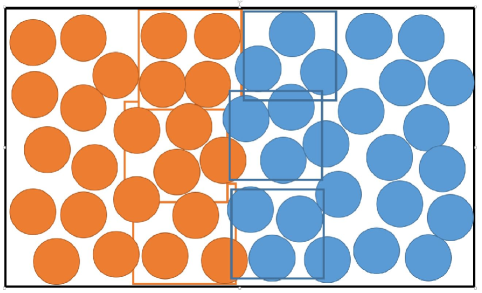
Figure 1: The scheme of the intrinsic density calculation for a water-hexane interface.

Figure 2 presents the intrinsic and non-intrinsic density profiles of water and n-hexane of a water-hexane planar interface obtained from atomistic simulations with the TIP4P2005-TraPPE and TIP4P2005-OPLSAA models. Both atomistic models result in the same water density profiles and very similar hexane density profiles. Also, both atomistic models can reproduce the experimental density of water and hexane at 310 K. The intrinsic density profiles show that there are two water layers close to the interface. In addition, the strong directional bonding of water creates a well-defined correlation structure at short distances from the interface, but it does not propagate to longer distances as efficiently as it does for more packed liquid structures such as alkanes. The comparison of Figure 2 (a) and (b) shows longer-range oscillations in alkanes than in water. Similar observations were made for a water-hexane binary system with the SPC/E water model.Bresme, Chacón, and Tarazona (2010) In the case of hexane, we see that the distribution of the first peak is wider. This is due to the long tail of the alkane molecule. Overall, we find that the intrinsic structure of the water/n-hexane system is insensitive to atomistic FF parameters.

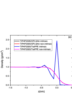
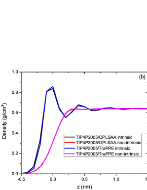
Figure 2: The intrinsic and non-intrinsic density profiles of (a) water and (b) hexane at the water-hexane interface as a function of $z$ obtained from atomistic simulation. The point $z=0$ corresponds to the position of the outermost water/hexane atoms in the intrinsic density profile and the Gibbs dividing surface of the water-hexane system for the non-intrinsic density profile.

The density profiles in CG simulations are shown in Figure 3. The non-intrinsic and intrinsic densities of water and hexane are different for various CG FFs. The non-intrinsic density profile obtained with the SAFT CG FF is flatter than the MARTINI CG FF. It should be noted that the density of water in the n-hexane phase in the atomistic simulations is negligibly small for the considered here TIP4P2005 water model (0 due to the float point precision in the atomistic simulations). In CG simulations, the density of water in hexane is 3$\times$10^-4 g/cm³ for the MARTINI CG FF that is approximately five times larger than the experimental value of 6$\times$10^-5 g/cm³.Roddy and Coleman (1968) For the SAFT bio2 CG water model in n-hexane, the water density is even greater. In Figure 3(a), the intrinsic water density profile has three peaks (two peaks were observed in MD simulations). This indicates that the CG water phase shows a longer-range ordered structure in comparison with the atomistic simulation. The intrinsic density profiles are similar for the original and polarized MARTINI CG water models, except that the original MARTINI CG water model has a higher interfacial density. The first peak in the SAFT bio2 CG model is lower than in the atomistic models because the CG model produces a wider interface. The positions of the first intrinsic density peaks for CG n-hexane models are also very close. The hexane intrinsic density profiles, obtained from the MARTINI and SAFT CG n-hexane models, do not have distinct peaks (Figure 3(b)). However, we can observe a peak in the hexane intrinsic density in the polarized MARTINI CG model. This is because single CG beads are used for both the MARTINI and SAFT bio2 CG water models. On the other hand, the polarized MARTINI CG water model has a physics-based three-point structure. Bresme et al. have demonstrated that the packing of water molecules will influence the orientation of alkane molecules at the interface.Bresme et al. (2008) In our CG simulations, we also see that the geometry topology constraint of the CG water model would affect the local surface structure of the hexane phase. For the SAFT n-hexane model, the CG water beads infiltrate into the hexane phase so deeply that the density of the first peak is lower than that of the bulk phase. In Figures 3 (a) and (b), the intrinsic density profiles of water or hexane are all different, which illustrates that the intrinsic density profile is sensitive to the choice of water and n-hexane CG models.

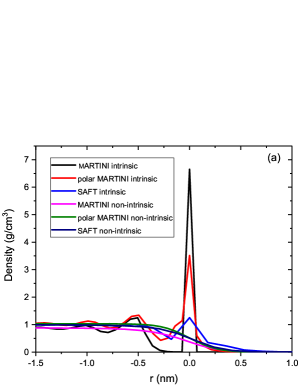
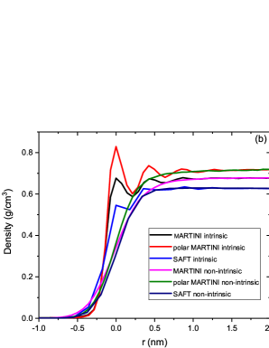
Figure 3: The intrinsic and non-intrinsic density profiles of (a) Water and (b) Hexane at the water-hexane interface in CG simulations. The zero point of the interface corresponds to the position of the outermost water/hexane atoms in the intrinsic density profile and the Gibbs dividing surface of the water-hexane system for the non-intrinsic density profile.

III.1.2 Pressure profiles and interfacial tension

Previous atomistic simulations demonstrated that the errors in the estimated surface tension and liquid density are closely correlated.Nicolas and Smit (2002); Underwood and Greenwell (2018) Therefore, the accurate prediction of density is very important in the calculation of surface tension. Above, we demonstrated that both considered atomistic water and hexane models can reproduce the liquid bulk density at 310 K. Here, we calculate the interfacial tension using the pressure tensor based on the mechanical approach.Irving and Kirkwood (1950); Ghoufi et al. (2008); Lovett and Baus (1997); Vanegas, Torres-Sánchez, and Arroyo (2014); Admal and Tadmor (2010) The details off calculating the pressure tensor components and the interfacial tension are given in Appendix B. The normal and tangent pressure tensor components as a function $z$, obtained from the atomistic and CG simulations, are presented in Figure 4 and Figure 5. There are two symmetrical positive stress regions in the tangent component of pressure, corresponding to the two water-hexane interfaces, in the atomistic simulations (Figure 4). They both appear on the water side of the interfaces. A similar pressure profile was also observed in an atomistic simulation with the TIP3P water and CHARMM hexane models.Nicolas and de Souza (2004) Water molecules cause interface polarization and the positive pressure region on the water side of the interface.

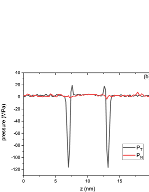
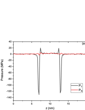
Figure 4: Pressure tensor components of the water-hexane planar interface in the atomistic (a) TIP4P2005 water + hexane in TraPPE FF and (b) TIP4P2005 water + hexane in OPLS-AA FF models.

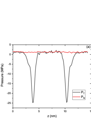
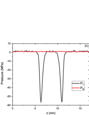
Figure 5: Local pressure components of water-hexane planar interface in (a) MARTINI FF, (b) MARTINI FF with polarized water, and (c) SAFT FF models.

Calculated and experimentally determined interfacial tensions are listed in Table LABEL:tableAAIT. Both atomistic models predict the interfacial tension within 5% of the experimental value. We note that the computational cost of the all-atom model (OPLS-AA FF) is about five times larger than that of the united-atom model (TraPPE FF). The SAFT CG FF can also reproduce the experimental interfacial tension. However, the interfacial tension predicted by the MARTINI CG FF is only half of the experiment value. A previous MARTINI CG FF simulation study of a water-octane system at 298 K also reported an approximately 25% error in the estimated interfacial tension.Neyt et al. (2014) In addition, we find that using the polarized MARTINI water model instead of the MARTINI water model only slightly improves the interfacial tension prediction.

Table 1: The interfacial tensions $\gamma_{0}$ of the water-hexane planar interface in the atomistic and CG simulations and the experimentZeppieri, Rodríguez, and López de Ramos (2001) at 310 K.

Model	Interfacial tension (mN/m)
Experiment	49.4
atomistic TIP4P2005+TraPPE	52.4$\pm$1.1
atomistic TIP4P2005+OPLS-AA	52.1$\pm$1.2
CG MARTINI	25.9$\pm$1.0
CG Polarized MARTINI	27.8$\pm$1.2
CG SAFT	51.6$\pm$1.1

III.2 Curved interface

Here, we model a 2 nm water droplet in hexane. In Section III.2.1, we present averaged density profiles as a function of the normal distance from the interface. In Section III.2.2, we show averaged pressure profiles as a function of the distance from the droplet center.

III.2.1 Density profiles

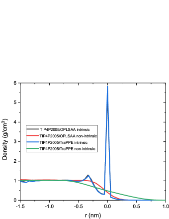
Figure 6: The intrinsic and non-intrinsic density profiles of a 2 nm water droplet in n-hexane obtained from atomistic simulations.

The intrinsic and non-intrinsic density profiles of a 2 nm water droplet in n-hexane, obtained in the two atomistic models, are shown in Figure 6. There are two peaks in the intrinsic density profiles in both atomistic models, which is similar to what we observed the planar interface atomistic simulations. However, the peaks at the curved interface are higher than those at the planar interface. Compared to Figure 2, we also see that the width of the first peak is narrower, implying that the first water layer on the droplet surface is thinner than the one at the planar interface.

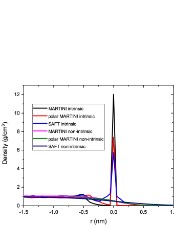
Figure 7: The intrinsic and non-intrinsic density profiles of a 2 nm water droplet in n-hexane obtained from CG simulations.

The CG water droplets show qualitatively different results. Figure 7 shows the density profiles of a 2 nm water droplet in n-hexane with various CG FFs. In the CG simulations of the planar interface, we see three density peaks on the water side. In Figure 7, the intrinsic density profile in the SAFT CG FF simulation has three peaks, while there are only two peaks for the MARTINI FF. This could be caused by a larger cutoff in the SAFT CG FF. Both, the CG and atomistic simulations show that the first peak in the water density profile is much higher for a curved interface than a planar interface.

III.2.2 Pressure profiles and interfacial tension

Although it is widely accepted that the Laplace law, relating the pressure jump across a curved interface to its curvature, fails for nanodroplets, the limit of the Laplace law validity is controversial. Takahashi and Morita concluded that this limit is less than 1 nm.Takahashi and Morita (2013) For liquid droplets in vapor environment, thid limit was found to be between 5–10 nm.Ghoufi and Malfreyt (2011); Malijevsky and Jackson (2012) Figures 8 and 9 show the normal and tangential components of the pressure tensor for a 2 nm water droplet in n-hexane. We see negative peaks in the tangent pressure profile at the interface in all simulations, indicating that the interface is under compression. Similar to the planar interface in atomistic simulations, we find a small peak on the water side of the tangent pressure in the droplet atomistic simulations. The pressure in the water droplet is greater than that in the hexane phase, which is consistent with the Laplace law. Comparing Figures 8 and 9, we find that the inner pressure in the atomistic simulations is higher than that in the CG simulations. In addition, electrostatic interactions in the MARTINI FF slightly increase the inner pressure, as shown in Figure 9(b).

Table LABEL:tab:2nmif lists the interfacial tensions of a 2 nm water droplet in n-hexane obtained from the atomistic and CG simulations. Both atomistic models result in a similar interfacial tension, which is smaller than the interfacial tension of the planar interface. Similar to the planar interface, the interfacial tension calculated with the MARTINI CG FFs is much smaller than that provided by the corresponding atomistic simulation. The SAFT CG FF, which is able to reproduce the interfacial tension of the planar interface, also results in a nearly 50 % smaller interfacial tension than that in the atomistic simulations.

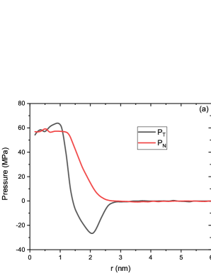
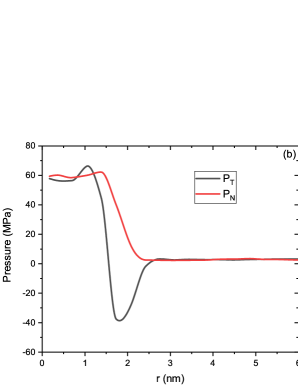
Figure 8: Pressure components as a function of the distance from the center of a 2 nm water droplet in n-hexane in atomistic FF simulations, including (a) TIP4P2005 water model and n-hexane in TraPPE FF and (b) TIP4P2005 water model and n-hexane in OPLS-AA FF.

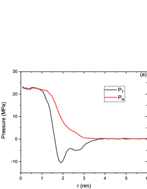
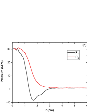
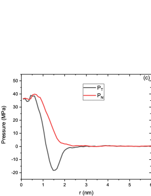
Figure 9: Pressure components as a function of the distance from the center of a 2 nm water droplet in n-hexane in CG FF simulations, including (a) MARTINI FF, (b) MARTINI FF with polarized water model and (c) SAFT FF models.

Table 2: The interfacial tensions $\gamma_{2}$ (R=2 nm) of a water droplet in n-hexane for various atomistic and CG FFs at 310 K.

Model	Interfacial tension (mN/m)
atomistic TIP4P2005+TraPPE	47.0$\pm$1.1
atomistic TIP4P2005+OPLS-AA	47.2$\pm$1.9
CG MARTINI	21.4$\pm$2.0
CG Polarized MARTINI	23.9$\pm$2.2
CG SAFT	27.7$\pm$1.1

IV estimation of the interaction parameters in CG FF using machine learning

Our results in the previous section show that the MARTINI CG FF cannot reproduce the interfacial tension and density profile near the interface observed in our atomistic simulations. The SAFT CG FF can predict the interfacial tension of the planar interface but underestimates the interfacial tension of the curved interface by almost 50%. In addition, we find that the SAFT CG FF overestimates the solubility of water in n-hexane. We hypothesize that one reason for the poor performance of the above tested CG FFs is that they use a relatively high degree of coarse graining. We therefore propose using the SDK CG FF Shinoda, Devane, and Klein (2007) as it allows a lower degree of coarse-graining. The current SDK model does not define the parameters of the water-hexane potential for the low coarse-graining degree water model. We note that there is an SDK FF for the high coarse-graining degree water model, but we find that this water model leads to crystallization of large water droplets.

In the remainder of this paper, we propose a new approach for learning coarse-grained potentials, apply it to estimating parameters in the water-hexane potential under the SDK CG FF framework, and test the resulting model for the water-hexane system against atomistic simulations. In this work, we use the 1:2 water model (one CG water bead represents two water molecules) and the 1:3 hexane model. The potential between CG water and hexane beads is given as

$$U_{\text{w-h}}=\left(\frac{\lambda_{r}}{\lambda_{r}-\lambda_{a}}\right)\left(\frac{\lambda_{r}}{\lambda_{a}}\right)^{\frac{\lambda_{a}}{\lambda_{r}-\lambda_{a}}}\varepsilon\left(\left(\frac{\sigma}{r}\right)^{\lambda_{r}}-\left(\frac{\sigma}{r}\right)^{\lambda_{a}}\right),$$ (1)

where $\lambda_{r}$ and $\lambda_{a}$ are repulsive and attractive exponents, $\varepsilon$ is the energy parameter, and $\sigma$ is the core diameter. The potentials $U_{\text{w-w}}$ and $U_{\text{h-h}}$ between water-water and hexane-hexane beads have the same form, with parameters $\lambda_{r}$, $\lambda_{a}$, $\sigma$, and $\varepsilon$ listed in Table LABEL:tab:cgpar. In the original SDK framework, there are only two combinations of $\lambda_{r}$ and $\lambda_{a}$, (12,4) and (9,6). The former combination results in a sharper interface because of the larger repulsive force corresponding to $\lambda_{r}=12$. In the atomistic simulations, we observe a relatively sharp water-hexane interface. Therefore, in the $U_{\text{w-h}}$ potential, we set $\lambda_{r}=12$ and $\lambda_{a}=4$. Next, we learn the $\sigma$ and $\varepsilon$ parameters in the $U_{\text{w-h}}$ potential using the surface tension of the planar and curved water-hexane interfaces as target properties.

Table 3: The CG interaction parameters of water and hexane.Shinoda, Devane, and Klein (2007); RN280

CG model	$\lambda_{r}$	$\lambda_{a}$	$\varepsilon$ (kcal/mol)	$\sigma$(nm)
Water	9	6	0.7050	0.2908
Hexane	9	6	0.4690	0.4585

We define the parameter vector $\theta=(\sigma,\varepsilon)^{T}$ and use polynomial regression (PR) (Xiu and Karniadakis, 2002; Lei et al., 2015; Li et al., 2016) to construct a surrogate model of the interfacial tension as a function of $\theta$. PR uses a linear combination of a set of orthogonal basis functions of $\theta$ to represent the quantity of interest (QoI) $f$:

$$f(\theta)=\sum_{i=1}^{N}c_{i}\psi_{i}(\theta),$$ (2)

where $\psi_{i}$ are basis functions (Legendre polynomials) and $c_{i}$ are constant coefficients. Here, $f$ is the interfacial tension obtained from the atomistic simulations.

We search parameters in the space $\sigma\in[\sigma_{min},\sigma_{max}]$ and $\varepsilon\in[\varepsilon_{min},\varepsilon_{max}]$ and treat $\sigma$ and $\varepsilon$ as independent uniform random variables given by

$$\left(\begin{array}[]{c}{\sigma}\\ {\varepsilon}\end{array}\right)=\left(\begin{array}[]{c}\overline{\sigma}\\ \overline{\varepsilon}\end{array}\right)+\left(\delta_{\sigma},\delta_{\varepsilon}\right)\cdot\left(\begin{array}[]{cc}{\xi_{1}}&0\\ 0&{\xi_{2}}\end{array}\right),$$ (9)

where $\left(\overline{\sigma},\overline{\varepsilon}\right)=(0.5,\ 0.225)$ are the parameter means and $(\xi_{1},\xi_{2})$ are independent random variables uniformly distributed on $[-1,1]$. The $\overline{\sigma}$ and $\overline{\varepsilon}$ values are defined as an average of $\sigma$ and $\varepsilon$ in water-water and hexane-hexane potentials, respectively. The parameters $\delta_{\sigma}=0.1$ and $\delta_{\varepsilon}=0.035$ are found as $\delta_{\sigma}=(\sigma_{max}-\overline{\sigma})$ and $\delta_{\varepsilon}=(\varepsilon_{max}-\overline{\varepsilon})$, where $\sigma_{max}=0.6$ is the maximum size of the water-hexane molecule cluster, and $\varepsilon_{max}=0.26$ is the interaction energy between water and hexane. $\sigma_{min}$ and $\varepsilon_{min}$ are computed as $\sigma_{min}=2\overline{\sigma}-\sigma_{max}$ and $\varepsilon_{min}=2\overline{\varepsilon}-\varepsilon_{max}$, respectively. We generate 49 samples of $\xi_{1}$ and $\xi_{2}$ using the sparse grids method Gerstner and Griebel (1998) with one-dimensional Gaussian quadrature points and the tensor product rule (i.e., the number of samples is equal to $7^{d}$, where $7$ is the number of one-dimensional quadrature points and $d$ is the number of unknown parameters). We then compute $(\sigma,\varepsilon)$ for each sample $(\xi_{1},\xi_{2})$ from Eq (9), simulate the flat interface using the CG model for these values of $(\sigma,\varepsilon)$, and compute the corresponding interfacial tension. The values of the interfacial tension are used to estimate the coefficients $c_{i}$ in the PR surrogate model (2) based on the probabilistic collocation method.Xiu and Hesthaven (2005) We find that the interfacial tension changes smoothly in the considered parameter space and the relative error of the surrogate model, based on 10-fold cross validation,Stone (1974) is less than 1%.

Finally, the surrogate model is used to find parameters $\sigma$ and $\varepsilon$ that correspond to the interfacial tension of the planar water-hexane interface in the atomistic simulation. Figure 10(a) shows $\frac{f_{0}(\sigma,\varepsilon)-\gamma_{0}}{\gamma_{0}}$ ($f_{0}(\sigma,\varepsilon)$ is the surrogate model for the interfacial tension of the planar interface, and $\gamma_{0}$ is the interfacial tension of the planar interface obtained from the atomistic simulation) as a function of $\sigma$ and $\varepsilon$. There is an infinite number of pairs $\left(\sigma,\varepsilon\right)$ that generate $\gamma_{0}$ lying on the curve $\frac{f_{0}(\sigma,\varepsilon)-\gamma_{0}}{\gamma_{0}}=0$. To make parameterization unique, we select the interfacial tension of a 2 nm water droplet in hexane ($\gamma(2)=\gamma_{2}=47mN/m$) as an additional constraint. We use the same 49 samples of random variables and the corresponding $\sigma$ and $\varepsilon$ to simulate a water droplet in hexane with the CG model. To reduce the statistical error caused by the thermal fluctuations of a small droplet, every sample is averaged over five independent CG simulations. These simulations are used to construct the surrogate model of the surface tension of a 2 nm droplet $f_{2}(\sigma,\varepsilon)$. Then, the optimal $\sigma$ and $\varepsilon$ are determined by solving the minimization problem:

$$(\sigma,\varepsilon)=\min_{\sigma,\varepsilon}\left[\sqrt{\left(\frac{f_{0}(\sigma,\varepsilon)-\gamma_{0}}{\gamma_{0}}\right)^{2}+\left(\frac{f_{2}(\sigma,\varepsilon)-\gamma_{2}}{\gamma_{2}}\right)^{2}}\right].$$ (10)

Figure 10(b) shows $\sqrt{\left(\frac{f_{0}(\sigma,\varepsilon)-\gamma_{0}}{\gamma_{0}}\right)^{2}+\left(\frac{f_{2}(\sigma,\varepsilon)-\gamma_{2}}{\gamma_{2}}\right)^{2}}$ as a function of $\sigma$ and $\varepsilon$. It can be seen that there are two sets of optimal parameters: $\varepsilon=0.23$ kcal/mol and $\sigma=0.48$ nm (the star); and $\varepsilon=0.19$ kcal/mol and $\sigma=0.59$ nm (the square). The difference between the response surface values at these two points is less than 2%, which is within the range of fluctuations observed in the CG simulations.

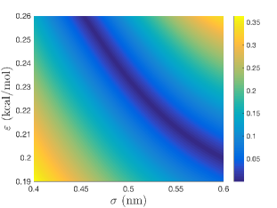
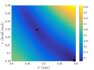
Figure 10: (a) $\frac{f_{0}(\sigma,\varepsilon)-\gamma_{0}}{\gamma_{0}}$ and (b) $\sqrt{\left(\frac{f_{0}(\sigma,\varepsilon)-\gamma_{0}}{\gamma_{0}}\right)^{2}+\left(\frac{f_{2}(\sigma,\varepsilon)-\gamma_{2}}{\gamma_{2}}\right)^{2}}$ versus $\sigma$ and $\varepsilon$.

Fluctuations in the value of the interfacial tension computed from the CG simulations are due to thermal fluctuations. When the interfacial tension is used as a target to estimate parameters, these fluctuations (which can be treated as uncertainty) should be transferred to parameters. This requires knowledge of the interfacial tension sensitivity with respect to the parameters $\sigma$ and $\varepsilon$. To perform the sensitivity analysis, we add 10% and 20% Gaussian noise to the values of the interfacial tension obtained from the 49 CG simulations, construct the surrogate model, and determine the optimal parameter set $(\varepsilon,\sigma)$ as described above. We repeat this procedure 100,000 times and compute the probability density function (PDF) of the optimal $(\varepsilon,\ \sigma)$. Figure 11 shows the PDFs of the $(\varepsilon,\sigma)$ parameter set. We see that the PDF maximum is at the position $\left(\varepsilon,\sigma\right)=(0.23,0.48)$ for both 10% and 20% added noise, with the peak in the 10% case being steeper than that in the 20% case. This is because the smaller noise (uncertainty) in the surface tension leads to a more certain estimate of the optimal parameters. The important feature of Figure 11 is that, unlike Figure 10, it predicts a unique set of the optimal parameters. The square in Figure 10 corresponds to a point with very small probability in Figure 11. With $\left(\varepsilon,\sigma\right)=(0.23,0.48)$, the CG model produces an interfacial tension of 53.2 mN/m for the planar interface and 42.0 mN/m for the curved interface: these are within 11% of the values obtained in atomistic simulations. Finally, we test the CG model with $\left(\varepsilon,\sigma\right)=(0.23,0.48)$, by simulating a 3 nm water droplet in n-hexane and find that the interfacial tension is 45.1 mN/m, which is within 9% of the 49.1 mN/m interfacial tension value computed from the atomistic simulation of the 3 nm water droplet.

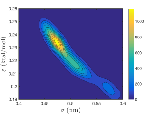
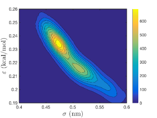
Figure 11: PDF function of the optimal parameter via UQ analysis of the CG interaction with various input noises. (a) 10% Gaussian noise and (b) 20% Gaussian noise.

The intrinsic and non-intrinsic density profiles for planar and curved interfaces obtained from the CG model with $\left(\varepsilon,\sigma\right)=(0.23,0.48)$ are presented in Figure 12. The comparison of Figures 12(a) and (b) with Figures 2(a) and (b) shows that the width of the planar interface is very similar in the atomistic and CG simulations, as well as in the resulting non-intrinsic density profiles for both water and hexane. For the planar interface, there are three peaks in the “CG” intrinsic density profile of water, while only two peaks are observed in the “atomistic” intrinsic water density profile. The CG FF produces a longer-range ordered structure because it uses a larger cutoff than the atomistic FF. On the other hand, the locations and magnitudes of the first two peaks in the CG density profile are close to those in the atomistic simulations. The comparison of Figures 12(c) and 6 also demonstrates good agreement between the the intrinsic and non-intrinsic density profiles of a 2 nm water droplet (i.e., curved interface) obtained with our CG model and the atomistic models in terms of the bulk water density, interface width, and structure. There are some disagreements in the intrinsic density profiles of hexane in the CG and atomistic simulations. There is a relatively small peak in the intrinsic atomistic hexane density profile and no apparent peak in the CG intrinsic hexane density profile. This disagreement is caused by the coarse-graining of the one-site CG water and two-site CG hexane models.

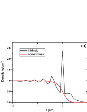
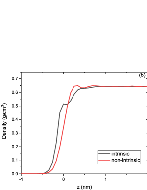
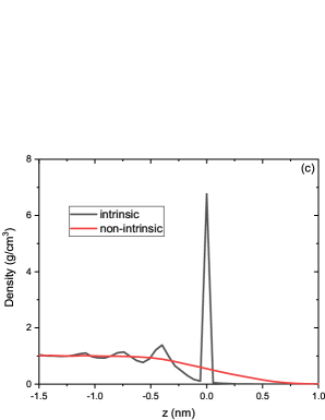
Figure 12: The intrinsic and non-intrinsic density profiles of a water-hexane interface obtained with the CG FF with learned $\sigma$ and $\varepsilon$. (a) Water at water-hexane planar interface. (b) Hexane at the water-hexane planar interface. (c) Water at the water-hexane curved interface.

V Conclusion

We proposed a new approach for parameterization of CG FF and used it to parameterize the SDK CG FF for water-hexane systems with the interfacial tension of planar and curved interfaces as target properties. We demonstrated that the proposed model significantly improves the accuracy of CG predictions of the coexisting densities, interface structure, and interfacial tension for planar and curved water-hexane interfaces.

We started this work by testing two atomistic FFs and three CG FFs for water-hexane systems, including a planar interface separating water and hexane and a water droplet in hexane. We found that the results of both atomistic FFs agree well with experiments and later used them as references. Next, we studied three popular CG FFs and found that none of them can accurately reproduce the interfacial structure and interfacial tension of planar and/or curved water-hexane interfaces.

Finally, we proposed a new approach for learning parameters in a CG FF with respect of target properties and used it to parameterize the SDK CG FF for water-hexane system using the surface tension of a planar interface and a 2 nm water droplet in hexane as target properties. We found that the proposed SDK CG FF can accurately describe the interface structure and predict the curvature-dependent interfacial tension of the water-hexane system. For the latter, we demonstrated that the CG model can estimate the interfacial tension of a 3 nm water droplet (in addition to the surface tension of a 2 nm droplet and planar interface that we used to train the CG model). The proposed approach can be easily generalized for learning parameters in other CG models of complex fluids using appropriate target properties.

Appendix A Non-intrinsic and intrinsic density profiles calculations

Non-intrinsic density profiles are calculated along the direction normal to the interface using a bin size of 0.2 nm. The non-intrinsic density is averaged within each bin over time. However, these non-intrinsic density profiles are subject to capillary waves due to thermal fluctuations. Recently, the intrinsic sampling method was developed to obtain the intrinsic density of liquid-vapor and liquid-liquid interfaces.Hantal et al. (2010); Bresme et al. (2008); Bresme, Chacon, and Tarazona (2008); Partay Livia et al. (2007) The capillary wave theory provides the dependence of a density profile on the interfacial area. This theory postulates that a liquid surface can be represented by the intrinsic surface $z=\ \xi(\mathbf{R},q)$. The intrinsic surface is defined in terms of a surface layer of $N$ molecules or molecular sites with coordinates $\mathbf{R}=\left(x,y\right)$ on the transverse plane. The vector $\mathbf{R}$ represents the instantaneous molecular border of the coexisting phases and depends on the the wave vector cutoff $q$, which defines the surface resolution. For a given $q$, the intrinsic density profile is defined as

$$\rho\left(z\right)=\frac{1}{A}\left\langle\sum_{i}{\delta(z-z_{i}+\gamma(x_{i},y_{i}))}\right\rangle,$$ (11)

where $z$ is the local non-intrinsic interface location, $A$ is the cross-section area of the interface, $\left\langle\cdots\right\rangle$ is the ensemble statistical average, and $\gamma$ is the amplitude of the thermal fluctuations.

We use the ITIM algorithmPartay Livia et al. (2007); Sega et al. (2016, 2013, 2018) for identifying the interfacial molecules that are exposed to the opposite phase using a probe sphere radius of 0.2 nm. The probe sphere is moved along test lines perpendicular to the plane of the fluid-fluid interface. Atoms that first encounter the probing ball are identified as the interfacial atoms, and the corresponding molecules are identified as the interfacial molecules. This process is repeated over the entire interfacial area in the simulation.

Appendix B Pressure profile and interfacial tension calculations

The interfacial tension of a planar interface is computed asLovett and Baus (1997)

$$\gamma(z)=\int_{-z/2}^{z/2}{(P_{N}\left(z\right)-P_{T}\left(z\right))dz}.$$ (12)

For a spheric droplet, the expression for the surface tension takes the form

$$\gamma(r)=\int_{0}^{\infty}{(P_{N}\left(r\right)-P_{T}\left(r\right))dr},$$ (13)

where $P_{N}$ and $P_{T}$ are the normal and tangential components of the pressure tensor along the normal direction to the surface. We use the Irving-Kirkwood Irving and Kirkwood (1950) and Vanegas and OllilaVanegas, Torres-Sánchez, and Arroyo (2014); Ollila et al. (2009) approaches for computing pressure components in Eqs (12) and (13), respectively. These approaches were originally proposed for pair-wise interactions. To calculate pressures due to three-body angle potentials, these potentials are decomposed into pair-wise potentials by the central force decomposition (CFD) method.Admal and Tadmor (2010) The many-body electrostatic interactions are approximated as pairwise interaction. In our pressure calculations, we use a pairwise potential with the 2.0 nm cutoff.

References

- Ishiyama, Imamura, and Morita (2014) T. Ishiyama, T. Imamura, and A. Morita, Chem. Rev. 114, 8447 (2014).
- Piradashvili et al. (2016) K. Piradashvili, E. M. Alexandrino, F. R. Wurm, and K. Landfester, Chem. Rev. 116, 2141 (2016).
- Liu, Li, and Shao (2011) S. J. Liu, Q. Li, and Y. H. Shao, Chem. Soc. Rev. 40, 2236 (2011).
- van der Spoel, van Maaren, and Caleman (2012) D. van der Spoel, P. J. van Maaren, and C. Caleman, Bioinformatics 28, 752 (2012).
- Mayoral and Goicochea (2013) E. Mayoral and A. G. Goicochea, J. Chem. Phys. 138, 7 (2013).
- Yesylevskyy et al. (2010) S. O. Yesylevskyy, L. V. Schafer, D. Sengupta, and S. J. Marrink, PPLOS Comput. Biol. 6 (2010), 10.1371/journal.pcbi.1000810.
- Lobanova et al. (2015) O. Lobanova, C. Avendano, T. Lafitte, E. A. Muller, and G. Jackson, Mol. Phys. 113, 1228 (2015).
- Lobanova et al. (2016) O. Lobanova, A. Mejia, G. Jackson, and E. A. Muller, J. Chem. Thermodyn. 93, 320 (2016).
- Shinoda, Devane, and Klein (2007) W. Shinoda, R. Devane, and M. L. Klein, Mol. Simulat. 33, 27 (2007).
- Marrink et al. (2007) S. J. Marrink, H. J. Risselada, S. Yefimov, D. P. Tieleman, and A. H. de Vries, J. Phys. Chem. B 111, 7812 (2007).
- Monticelli et al. (2008) L. Monticelli, S. K. Kandasamy, X. Periole, R. G. Larson, D. P. Tieleman, and S. J. Marrink, J. Chem. Theory. Comput. 4, 819 (2008).
- Ghoufi, Malfreyt, and Tildesley (2016) A. Ghoufi, P. Malfreyt, and D. J. Tildesley, Chem. Soc. Rev. 45, 1387 (2016).
- Zubillaga et al. (2013) R. A. Zubillaga, A. Labastida, B. Cruz, J. C. Martínez, E. Sánchez, and J. Alejandre, J. Chem. Theory Comput. 9, 1611 (2013).
- John and Csanyi (2017) S. T. John and G. Csanyi, J. Phys. Chem. B 121, 10934 (2017).
- Sidky and Whitmer (2018) H. Sidky and J. K. Whitmer, J. Chem. Phys. 148, 104111 (2018).
- Chmiela et al. (2018) S. Chmiela, H. E. Sauceda, K.-R. Müller, and A. Tkatchenko, Nat. Commun. 9, 3887 (2018).
- Tang, Zhang, and Karniadakis (2018) Y.-H. Tang, D. Zhang, and G. E. Karniadakis, J. Chem. Phys. 148, 034101 (2018).
- Underwood and Greenwell (2018) T. R. Underwood and H. C. Greenwell, Sci. Rep. 8, 11 (2018).
- Abascal and Vega (2005) J. L. F. Abascal and C. Vega, J. Chem. Phys. 123, 234505 (2005).
- Martin and Siepmann (1998) M. G. Martin and J. I. Siepmann, J. Phys. Chem. B 102, 2569 (1998).
- Neyt et al. (2014) J. C. Neyt, A. Wender, V. Lachet, A. Ghoufi, and P. Malfreyt, J. Chem. Theory. Comput. 10, 1887 (2014).
- Ashbaugh, Liu, and Surampudi (2011) H. S. Ashbaugh, L. Liu, and L. N. Surampudi, J. Chem. Phys. 135, 054510 (2011).
- Kaminski and Jorgensen (1996) G. Kaminski and W. L. Jorgensen, J. Phys. Chem. 100, 18010 (1996).
- Shi and Guo (2010) W.-X. Shi and H.-X. Guo, J. Phys. Chem. B 114, 6365 (2010).
- Hess et al. (1997) B. Hess, H. Bekker, H. J. C. Berendsen, and J. G. E. M. Fraaije, J. Comput. Chem. 18, 1463 (1997).
- Biscay et al. (2009) F. Biscay, A. Ghoufi, F. Goujon, V. Lachet, and P. Malfreyt, J. Chem. Phys. 130, 184710 (2009).
- Mitrinović et al. (2000) D. M. Mitrinović, A. M. Tikhonov, M. Li, Z. Huang, and M. L. Schlossman, Phys. Rev. Lett. 85, 582 (2000).
- Hantal et al. (2010) G. Hantal, M. Darvas, L. B. Partay, G. Horvai, and P. Jedlovszky, J. Phys. Condens. Matter 22 (2010), 10.1088/0953-8984/22/28/284112.
- Bresme et al. (2008) F. Bresme, E. Chacón, P. Tarazona, and K. Tay, Phys. Rev. Lett. 101, 056102 (2008).
- Bresme, Chacon, and Tarazona (2008) F. Bresme, E. Chacon, and P. Tarazona, Phys. Chem. Chem. Phys. 10, 4704 (2008).
- Partay Livia et al. (2007) B. Partay Livia, G. Hantal, P. Jedlovszky, r. Vincze, and G. Horvai, J. Comput. Chem. 29, 945 (2007).
- Bresme, Chacón, and Tarazona (2010) F. Bresme, E. Chacón, and P. Tarazona, Mol. Phys. 108, 1887 (2010).
- Roddy and Coleman (1968) J. W. Roddy and C. F. Coleman, Talanta 15, 1281 (1968).
- Nicolas and Smit (2002) J. P. Nicolas and B. Smit, Mol. Phys. 100, 2471 (2002).
- Irving and Kirkwood (1950) J. H. Irving and J. G. Kirkwood, J. Chem. Phys. 18, 817 (1950).
- Ghoufi et al. (2008) A. Ghoufi, F. Goujon, V. Lachet, and P. Malfreyt, Phys. Rev. E. 77, 031601 (2008).
- Lovett and Baus (1997) R. Lovett and M. Baus, J. Chem. Phys. 106, 635 (1997).
- Vanegas, Torres-Sánchez, and Arroyo (2014) J. M. Vanegas, A. Torres-Sánchez, and M. Arroyo, J. Chem. Theory Comput. 10, 691 (2014).
- Admal and Tadmor (2010) N. C. Admal and E. B. Tadmor, J. Elasticity. 100, 63 (2010).
- Nicolas and de Souza (2004) J. P. Nicolas and N. R. de Souza, J. Chem. Phys. 120, 2464 (2004).
- Zeppieri, Rodríguez, and López de Ramos (2001) S. Zeppieri, J. Rodríguez, and A. L. López de Ramos, J. Chem. Eng. Data 46, 1086 (2001).
- Takahashi and Morita (2013) H. Takahashi and A. Morita, Chem. Phys. Lett. 573, 35 (2013).
- Ghoufi and Malfreyt (2011) A. Ghoufi and P. Malfreyt, J. Chem. Phys. 135, 104105 (2011).
- Malijevsky and Jackson (2012) A. Malijevsky and G. Jackson, J. Phys. Condens. Matter 24, 464121 (2012).
- Xiu and Karniadakis (2002) D. Xiu and G. Karniadakis, SIAM J. Sci. Comput. 24, 619 (2002).
- Lei et al. (2015) H. Lei, X. Yang, B. Zheng, G. Lin, and N. A. Baker, Multiscale Model Sim. 13, 1327 (2015).
- Li et al. (2016) Z. Li, X. Bian, X. Yang, and G. E. Karniadakis, J. Chem. Phys. 145, 044102 (2016).
- Gerstner and Griebel (1998) T. Gerstner and M. Griebel, Numer. Algorithms. 18, 209 (1998).
- Xiu and Hesthaven (2005) D. Xiu and J. Hesthaven, SIAM J. Sci. Comput. 27, 1118 (2005).
- Stone (1974) M. Stone, J. R. Stat. Soc. Series. B. 36, 111 (1974).
- Sega et al. (2016) M. Sega, B. Fábián, G. Horvai, and P. Jedlovszky, J. Phys. Chem. C 120, 27468 (2016).
- Sega et al. (2013) M. Sega, S. S. Kantorovich, P. Jedlovszky, and M. Jorge, J. Chem. Phys. 138, 044110 (2013).
- Sega et al. (2018) M. Sega, G. Hantal, B. Fábián, and P. Jedlovszky, J. Comput. Chem. 39, 2118 (2018).
- Ollila et al. (2009) O. H. S. Ollila, H. J. Risselada, M. Louhivuori, E. Lindahl, I. Vattulainen, and S. J. Marrink, Phys. Rev. Lett. 102, 078101 (2009).