YITP-19-59
Numerical and analytical analyses of a matrix model with non-pairwise contracted indices

We study a matrix model that has $\phi_{a}^{i}\ (a=1,2,\ldots,N,\ i=1,2,\ldots,R)$ as its dynamical variable, whose lower indices are pairwise contracted, but upper ones are not always done so. This matrix model has a motivation from a tensor model for quantum gravity, and is also related to the physics of glasses, because it has the same form as what appears in the replica trick of the spherical $p$-spin model for spin glasses, though the parameter range of our interest is different. To study the dynamics, which in general depends on $N$ and $R$, we perform Monte Carlo simulations and compare with some analytical computations in the leading and the next-leading orders. A transition region has been found around $R\sim N^{2}/2$, which matches a relation required by the consistency of the tensor model. The simulation and the analytical computations agree well outside the transition region, but not in this region, implying that some relevant configurations are not properly included by the analytical computations. With a motivation coming from the tensor model, we also study the persistent homology of the configurations generated in the simulations, and have observed its gradual change from $S^{1}$ to higher dimensional cycles with the increase of $R$ around the transition region.

1 Introduction

Quantization of gravity is one of the major fundamental problems in theoretical physics. The quantization of general relativity by the standard perturbative methods of quantum field theory fails due to non-renormalizable divergences. Various approaches have been proposed and being studied to solve the fundamental problem, depending on views of authors. In one approach, general relativity (with higher derivative terms) is directly quantized as quantum field theory with the modern technique of the functional renormalization group [1]. In other approaches, fundamental discreteness is introduced to represent spacetimes, which include (causal) dynamical triangulations [2], loop quantum gravity [3], causal sets [4], quantum graphity [5], matrix models [6, 7, 8, 9, 10], tensor models [11, 12, 13, 14], and so on. In these discretized approaches, an important criterion for success is whether macroscopic spacetimes are generated, or in other words, whether there exist appropriate continuum limits that recover the usual continuum picture of spacetime with dynamics described by general relativity as low-energy effective theory.

The criterion above can in principle be checked by studying the properties of a wave function of each theory. If the wave function has a peak at a configuration that can well be described by a macroscopic spacetime picture, then the model can be considered to be potentially successful. An indirect motivation for the present paper is to understand the properties of the wave function [15] that is an exact solution to a tensor model in the Hamilton formalism [16, 17] (See Appendix A for the tensor model.). It has been argued and shown for some simple cases that the wave function has peaks at the tensor values that are invariant under Lie groups [18]. By using the correspondence developed in [19] between tensor values and spaces with geometries, this would imply that the spacetimes symmetric under Lie groups are favored quantum mechanically. However, the main difficulty in arguing this is that only little part of the peak structure (often called landscape in such contexts) of the wave function is known, not enough to discuss “probabilities of spacetimes.”

To simplify the problem keeping the main structure from the tensor model as much as possible, one of the authors of the present paper and his collaborators considered the following two simplifications in the former papers. One is that they considered a toy wave function rather than the actual wave function of the tensor model [20]. The actual wave function is expressed by a certain power, say $R$-th, of a function expressed by an integration over $N+1$ variables, but, in the toy wave function, the function is simplified to the one expressed by an integration over $N$ variables by fixing a certain integration variable to a constant. While this substantially simplifies the analysis, the toy wave function keeps the most crucial property mentioned above that there appear peaks at the tensor values that are symmetric under Lie groups as the actual wave function of the tensor model does [20].

Though this toy wave function is simpler than the actual one, it is still difficult to perform thorough analyses, because the dimension of the argument (a symmetric tensor with three indices) of the wave function is very large with the order of $\sim N^{3}/6$. Therefore, as an additional simplification, the authors in [21] considered a model that can be obtained by integrating over the argument of the toy wave function. This gives a dynamical system of a matrix, say $\phi_{a}^{i}\ (a=1,2,\ldots,N,\ i=1,2,\cdots,R)$, rectangular in general, where the lower indices are pairwise contracted, but the upper ones are not always done so. While this model does not fall into the known solvable models such as the rectangular matrix models [22, 23, 24] or the vector models [25, 26], it has the same form as what appears when the replica trick is applied to the spherical $p$-spin model for spin glasses [27, 28], where $R$ plays the role of the replica number. Here, though the form is exactly so, the concerned ranges of the dynamical variables and the parameters are different between our model and the spin glass model, and it seems reasonable to reanalyze the matrix model with fresh eyes: (i) While the replica number $R$ is taken to the vanishing limit in the replica trick, it takes a finite value $R\sim N^{2}/2$ in the correspondence to the tensor model, and should rather be taken to infinity in the thermodynamic limit $N\rightarrow\infty$; (ii) A coupling constant takes the opposite sign in our model compared to the spin glass model; (iii) There is a spherical constraint on the dynamical variable in the spherical $p$-spin model, but there is none in our model.

In this paper, we numerically study the matrix model by the Monte Carlo simulation with the standard Metropolis update method. This contrasts with the perturbative analytical computations performed in the previous paper [21]. We also perform some additional analytical computations to compare with the numerical results. We have obtained the following main results:

• The expectation values of some observables are computed by the numerical simulations, and it is observed that there exists a transition region around $R\sim N^{2}/2$. Intriguingly, the location is in good coincidence with $R=(N+2)(N+3)/2$ that is required by the consistency of the tensor model (Namely, the hermiticity of the Hamiltonian constraints. See Appendix A for more details.) [18, 15, 29]. Presently, this coincidence is mysterious, since there are no apparent connections between the transition and the consistency. The observables seem to continuously but substantially change their behavior at the transition region, but it has not been determined whether this transition is a phase transition or a crossover in the thermodynamic limit $N\rightarrow\infty$. The method for the Monte Carlo simulations performed in this paper is not powerful enough for the determination because of an issue explained below.

• The expectation values of some observables are analytically computed in the leading order, mostly based on the treatment in the previous paper [21], and are compared with the numerical results. Good agreement between them is obtained outside the vicinity of the transition region, while there exist deviations in the transition region. The deviations are such that they soften the transition to make it look more like a crossover. A next-leading order computation has also been performed, but this does not well correct the deviations.

• The tensor model suggests the presence of topological characteristics for the dominant configurations of the matrix $\phi_{a}^{i}$ (See Section 7 and Appendix A.). Therefore, we have studied topological characters of the configurations that are generated in the simulations by using the modern technique called persistent homology [30] in the topological data analysis. This technique extracts homology groups possessed by a data, which is a value of the matrix $\phi_{a}^{i}$ in our case. The dominant topology gradually changes from $S^{1}$ to higher-dimensional cycles with the increase of $R$ in the vicinity of the transition region.

• The Monte Carlo simulation becomes substantially difficult in the region with $R\gtrsim N^{2}/2$ and large $\lambda/k^{3}$, where $\lambda$ and $k$ are the parameters of our model (1). In the region, the step sizes of the Metropolis updates chosen for reasonable acceptance rates become too small to reach thermal equilliburiums in $\sim 10^{10}$ Metropolis updates.

• A characterization of the transition can be done by the sizes of the matrix elements, which take relatively large values at the region with $R\gtrsim N^{2}/2$ and large $\lambda/k^{3}$, but otherwise fluctuate around small values. In the former case, our model may behave like the spherical $p$-spin model, since the matrix elements are effectively constrained to non-zero sizes, which would approximately realize the spherical constraint in the spherical $p$-spin model. This may partly explain the bad performance of the Monte Carlo simulation in the region, seemingly reflecting the high viscous nature of glassy fluids.

This paper is organized as follows. In Section 2, we define the model and summarize the previous results [21] that are relevant to the present paper. In Section 3, some observables are introduced and the analytical expressions of their expectation values are obtained in a leading order. In Section 4, the details of the computation in the leading order are given. The result of the next-leading order is also presented, while the details of the computation are given in Appendix D. In Section 5, we perform a saddle point analysis of the expectation values of the observables in the leading order. This describes the transition as a continuous phase transition in the large $N$ limit, where the first derivatives of the expectation values of the observables with respect to $R$ are discontinuous. In Section 6, we compare the Monte Carlo and the analytical results. They agree well outside the transition region. In the transition region, however, there exist deviations, which smoothen the transition to make it look more like a crossover. In Section 7, we analyze the homology structure of the configurations generated by the simulations. The preference changes from $S^{1}$ to higher-dimensional cycles with the increase of $R$ in the vicinity of the transition region. The last section is devoted to a summary and future prospects. In Appendix A, the motivation for the matrix model is explained from the viewpoint of the tensor model. In Appendix B, an instructive computation of the partition function for $R=2$ is given. In Appendix C, Appendix D, and Appendix E, some equations used in the main text are explicitly derived. In Appendix F, a brief introduction to persistent homology is given.

2 The model

The partition function of our matrix model is given by

$$Z_{N,R}(\lambda,k):=\int_{{\mathbb{R}}^{NR}}d\phi\ \exp\left(-\lambda U(\phi)-k\hbox{Tr}(\phi^{t}\phi)\right),$$ (1)

where $\lambda$ and $k$ are the coupling constants assumed to be positive, $\phi$ is a (generally rectangular) real matrix, $\phi_{a}^{i}\ (a=1,2,\ldots,N,\ i=1,2,\ldots,R$), and $d\phi:=\prod_{a,i=1}^{N,R}d\phi_{a}^{i}$. The integration is over the $NR$-dimensional real space denoted by ${\mathbb{R}}^{NR}$. The coupling terms are defined by

$$\begin{split}&U(\phi):=\sum_{i,j=1}^{R}\left(\phi_{a}^{i}\phi_{a}^{j}\right)^{3},\\ &{\rm Tr}(\phi^{t}\phi):=\sum_{i=1}^{R}\phi_{a}^{i}\phi_{a}^{i},\end{split}$$ (2)

where the repeated lower indices are assumed to be summed over. We use this standard convention for the lower indices throughout this paper, unless otherwise stated. On the other hand, we do not use this convention for the upper indices: A sum over them must always be written explicitly. The background motivation for the matrix model is explained in Appendix A from the viewpoint of the tensor model.

In (2), the lower indices are contracted pairwise, while the upper indices are not necessarily so. Therefore the model has the symmetry of the $O(N)$ transformation on the lower indices, but only the permutation symmetry $S_{R}$ of relabeling $\{1,2,\ldots,R\}$ on the upper indices. These symmetries are not enough to diagonalize $\phi_{a}^{i}$ in general, and therefore this model cannot be solved in a similar way as the usual matrix model.

In the previous paper [21], we considered an expression which can just be obtained by separating the radial and angular part of the integration in (1): By the change of variable, $\phi_{a}^{i}=r\tilde{\phi}_{a}^{i}$, with $r^{2}=\sum_{i=1}^{R}\phi_{a}^{i}\phi_{a}^{i}$ and $\tilde{\phi}$ representing the angular coordinates, we obtain

$$Z_{N,R}(\lambda,k)=V_{NR-1}\int_{0}^{\infty}dr\,r^{NR-1}f_{N,R}(\lambda\,r^{6})\,e^{-k\,r^{2}},$$ (3)

where

$$f_{N,R}(t):=\frac{1}{V_{NR-1}}\int_{S^{NR-1}}d\tilde{\phi}\,e^{-t\,U(\tilde{\phi})}$$ (4)

with $V_{NR-1}=\int_{S^{NR-1}}d\tilde{\phi}$, the volume of the $NR-1$-dimensional unit sphere.

This rather trivial change of expression is actually very useful, because $f_{N,R}(t)$ can be shown to be an entire function of $t$ and therefore has a Taylor expansion in $t$ with the infinite convergence radius around $t=0$ (actually around arbitrary $t\neq\infty$). Therefore, in principle, the dynamics can be solved by obtaining the entire perturbative series of $f_{N,R}(t)$. Note that the corresponding perturbative expansion of $Z_{N,R}(\lambda,k)$ in $\lambda$ around $\lambda=0$, often obtained by perturbative methods, is merely an asymptotic series, because $Z_{N,R}(\lambda,k)$ has an essential singularity at $\lambda=0$. The $f_{N,R}(t)$ has also the property that it is a decreasing positive function of $t$ with $f_{N,R}(0)=1$ for real $t$. This property provides a good criterion for assessing the validity of an approximation of $f_{N,R}(t)$. In the previous paper [21], $f_{N,R}(t)$ in the leading order of $1/R$ has been determined by a Feynman diagrammatic method with the result,

$$\begin{split}&f^{1/R,{\rm leading}}_{N,R}(t)=\left(1+\frac{12t}{N^{3}R^{2}}\right)^{-\frac{N(N-1)(N+4)}{12}}\left(1+\frac{6(N+4)t}{N^{3}R^{2}}\right)^{-\frac{N}{2}}.\end{split}$$ (5)

In particular, (5) indeed satisfies the properties above: It is a decreasing function for real $t$ with $f^{1/R,{\rm leading}}_{N,R}(0)=1$, and is almost an entire function, since the locations of the singularities are far away from the relevant region $t\geq 0$ for large $N,R$.

Since there are two parameters $N,R$, which can be taken large, the range of validity of (5), which was derived in the leading order of $1/R$, is not obvious. However, in later sections, we will find that (5) will give results which agree well with those of the numerical simulations except in the transition region around $R\sim N^{2}/2$.

3 Observables

The purpose of this section is to introduce some observables, say $\cal O(\phi)$, and discuss the expectation values defined by

$$\langle{\cal O(\phi)}\rangle:=\frac{1}{Z_{N,R}(\lambda,k)}\int_{{\mathbb{R}}^{NR}}d\phi\ {\cal O}(\phi)\ e^{-\lambda U(\phi)-k{\rm Tr}(\phi^{t}\phi)}.$$ (6)

The observables must respect the symmetry $O(N)\times S_{R}$ mentioned in Section 2. Among various possibilities, we consider $\hbox{Tr}(\phi^{t}\phi)$ and $U(\phi)$ in (2), and also

$$U_{d}(\phi):=\sum_{i=1}^{R}\left(\phi_{a}^{i}\phi_{a}^{i}\right)^{3}.$$ (7)

The last one is the diagonal part of the sum in $U(\phi)$ in (2). Since these observables are some parts contained in the exponent of (1), they can be implemented in the numerical simulations with little additional computational costs.

To compute the expectation values of these observables, it is convenient to extend (1) by introducing the coupling constant $\lambda_{d}$ conjugate to $U_{d}(\phi)$ as

$$Z_{N,R}(\lambda,\lambda_{d},k):=\int_{{\mathbb{R}}^{NR}}d\phi\ e^{-\lambda U(\phi)-\lambda_{d}U_{d}(\phi)-k{\rm Tr}(\phi^{t}\phi)}.$$ (8)

Then the expectation values can respectively be expressed as

$$\begin{split}&\langle\hbox{Tr}(\phi^{t}\phi)\rangle=\frac{\partial}{\partial k}F_{N,R}(\lambda,\lambda_{d}=0,k),\\ &\langle U(\phi)\rangle=\frac{\partial}{\partial\lambda}F_{N,R}(\lambda,\lambda_{d}=0,k),\\ &\langle U_{d}(\phi)\rangle=\left.\frac{\partial}{\partial\lambda_{d}}F_{N,R}(\lambda,\lambda_{d},k)\right|_{\lambda_{d}=0},\end{split}$$ (9)

where $F_{N,R}(\lambda,\lambda_{d},k):=-\log Z_{N,R}(\lambda,\lambda_{d},k)$, which is the free energy of the model. Here we have put $\lambda_{d}=0$ at last, since our interest is in (1) corresponding to $\lambda_{d}=0$ of (8).

To compute the partition function (8), it is convenient to first separate the radial and the angular part as in (3):

$$Z_{N,R}(\lambda,\lambda_{d},k)=V_{NR-1}\int_{0}^{\infty}dr\ r^{NR-1}f_{N,R,\lambda,\lambda_{d}}(r^{6})\,e^{-kr^{2}},$$ (10)

where

$$f_{N,R,\lambda,\lambda_{d}}(t):=\frac{1}{V_{NR-1}}\int_{S^{NR-1}}d\tilde{\phi}\ e^{-\lambda\,t\,U(\tilde{\phi})-\lambda_{d}\,t\,U_{d}(\tilde{\phi})}.$$ (11)

The $f_{N,R,\lambda,\lambda_{d}}(t)$ has the similar properties as $f_{N,R}(t)$ explained in Section 2: It is an entire function of $t$; For $\lambda>0,\lambda_{d}\geq 0$, it is positive and decreasing in $t$ for real $t$; $f_{N,R,\lambda,\lambda_{d}}(0)=1$. With $f_{N,R,\lambda,\lambda_{d}}(t)$, the observables (9) can be expressed by

$$\begin{split}&\langle\hbox{Tr}(\phi^{t}\phi)\rangle=\frac{1}{{\cal N}_{f}}\int_{0}^{\infty}dr\ r^{NR+1}f_{N,R,\lambda,0}(r^{6})\,e^{-kr^{2}},\\ &\langle U(\phi)\rangle=-\frac{1}{{\cal N}_{f}}\int_{0}^{\infty}dr\ r^{NR-1}\frac{\partial}{\partial\lambda}f_{N,R,\lambda,0}(r^{6})\,e^{-kr^{2}},\\ &\langle U_{d}(\phi)\rangle=-\frac{1}{{\cal N}_{f}}\int_{0}^{\infty}dr\ r^{NR-1}\left.\frac{\partial}{\partial\lambda_{d}}f_{N,R,\lambda,\lambda_{d}}(r^{6})\right|_{\lambda_{d}=0}\,e^{-kr^{2}},\end{split}$$ (12)

where the normalization is given by

$${\cal N}_{f}=\int_{0}^{\infty}dr\ r^{NR-1}f_{N,R,\lambda,0}(r^{6})\,e^{-kr^{2}}.$$ (13)

From the leading order computation, which is detailed in Section 4, we obtain

$$f^{leading}_{N,R,\lambda,\lambda_{d}}(t)=h_{N,R}(\lambda Rt+\lambda_{d}t)\ h_{N,R}(\lambda_{d}t)^{R-1}$$ (14)

with

$$h_{N,R}(x):=\left(1+12\gamma_{3}x\right)^{-\frac{N(N-1)(N+4)}{12}}\left(1+6(N+4)\gamma_{3}x\right)^{-\frac{N}{2}},$$ (15)

where

$$\gamma_{n}:=\frac{\Gamma\left(\frac{NR}{2}\right)}{2^{n}\Gamma\left(\frac{NR}{2}+n\right)}.$$ (16)

When $\lambda_{d}=0$ is taken, (14) becomes

$$\begin{split}&f^{leading}_{N,R,\lambda,0}(t)=\left(1+12\gamma_{3}\lambda Rt\right)^{-\frac{N(N-1)(N+4)}{12}}\left(1+6(N+4)\gamma_{3}\lambda Rt\right)^{-\frac{N}{2}}.\end{split}$$ (17)

This could be expected to agree with (5), but there is a slight difference coming from (16) with $n=3$. This difference originates from the fact that the strategy of the computation we take in Section 4 is different from the one taken previously in [21], and therefore the expressions of the leading orders are slightly different from each other. However, they agree with each other in the leading order of $1/R$, since $\gamma_{n}\sim(NR)^{-n}$ for $NR\gg n$, as expected.

By putting these expressions into (12), we obtain

$$\begin{split}&\langle\hbox{Tr}(\phi^{t}\phi)\rangle_{leading}=\frac{1}{{\cal N}_{f}}\int_{0}^{\infty}dr\ r^{NR+1}f_{N,R,\lambda,0}^{leading}(r^{6})\,e^{-kr^{2}},\\ &\langle U(\phi)\rangle_{leading}=-\frac{R}{{\cal N}_{f}}\int_{0}^{\infty}dr\ r^{NR+5}\frac{h_{N,R}^{\prime}(\lambda Rr^{6})}{h_{N,R}(\lambda Rr^{6})}f_{N,R,\lambda,0}^{leading}(r^{6})\,e^{-kr^{2}},\\ &\langle U_{d}(\phi)\rangle_{leading}=-\frac{1}{{\cal N}_{f}}\int_{0}^{\infty}dr\ r^{NR+5}\left(\frac{h_{N,R}^{\prime}(\lambda Rr^{6})}{h_{N,R}(\lambda Rr^{6})}+(R-1)\frac{h_{N,R}^{\prime}(0)}{h_{N,R}(0)}\right)f_{N,R,\lambda,0}^{leading}(r^{6})\,e^{-kr^{2}},\end{split}$$ (18)

where ${\cal N}_{f}$ is given by (13) with $f_{N,R,\lambda,0}^{leading}(t)$. The actual values of these integrations can be obtained numerically.

4 Computations of $f_{N,R,\lambda,\lambda_{d}}(t)$ in the leading and the next-leading orders

In this section, we will compute $f_{N,R,\lambda,\lambda_{d}}(t)$ in the leading order of $t$, and will also show the result in the next-leading order, whose detailed computations are given in Appendix D. In [21], the computation in the leading order of $1/R$ has been performed by using the Feynman diagrams for the $\phi_{a}^{i}$ variables. In this paper, however, we will take a different strategy. This is because the new strategy makes more transparent the rather complicated counting of combinatorics performed in [21], and make it straightforward to include the extra coupling $\lambda_{d}U_{d}(\phi)$ and also to consider the next order in $t$. For $\lambda_{d}=0$, the new strategy gives essentially the same result as [21] in the leading order, as commented below (17).

Let us define

$$f_{N,R,\Lambda_{ij}}(t):=\frac{1}{V_{NR-1}}\int_{S^{NR-1}}d\tilde{\phi}\ e^{-t\,U_{\Lambda_{ij}}(\tilde{\phi})},$$ (19)

where

$$U_{\Lambda_{ij}}(\tilde{\phi}):=\sum_{i,j=1}^{R}\Lambda_{ij}\left(\tilde{\phi}_{a}^{i}\tilde{\phi}_{a}^{j}\right)^{3}$$ (20)

with a real symmetric matrix $\Lambda_{ij}$. The eigenvalues of the matrix $\Lambda_{ij}$ are assumed to be non-negative for the convergence of the corresponding partition function. The $f_{N,R,\Lambda_{ij}}(t)$ also has the same nice properties as $f_{N,R}(t)$ that it is an entire function, which has a Taylor series expansion in $t$ with the infinite convergence radius around $t=0$, and is a decreasing positive function of $t$ for real $t$ and $\Lambda\neq 0$ with $f_{N,R,\Lambda_{ij}}(0)=1$. If we take $\Lambda_{ij}=\lambda+\lambda_{d}\delta_{ij}$, (19) gives $f_{N,R,\lambda,\lambda_{d}}(t)$ in (11). By introducing a new variable $P_{abc}^{i}\ (a,b,c=1,2,\ldots,N,\ i=1,2,\ldots,R)$, which is symmetric for the lower indices, one can rewrite (19) as

$$\begin{split}&f_{N,R,\Lambda_{ij}}(t)\\ &=const.\int_{S^{NR-1}}d\tilde{\phi}\int_{-\infty}^{\infty}\prod_{i=1}^{R}\prod_{a\leq b\leq c=1}^{N}dP_{abc}^{i}\exp\left(-\sum_{i=1}^{R}P_{abc}^{i}P_{abc}^{i}+2I\sqrt{t}\sum_{i,j=1}^{R}\tilde{\Lambda}_{ij}P^{i}_{abc}\tilde{\phi}_{a}^{j}\tilde{\phi}_{b}^{j}\tilde{\phi}_{c}^{j}\right),\end{split}$$ (21)

where $I$ denotes the imaginary unit and $\tilde{\Lambda}_{ij}$ is a symmetric matrix satisfying,

$$\Lambda_{ij}=\sum_{k=1}^{R}\tilde{\Lambda}_{ik}\tilde{\Lambda}_{kj}.$$ (22)

The constant prefactor in (21) can be determined by $f_{N,R,\Lambda_{ij}}(0)=1$.

To compute (21), let us first integrate over $\tilde{\phi}$. This change of the order of the integrations can be done, because the integration over $P^{i}_{abc}$ with the infinite integration region converges uniformly for any $\tilde{\phi}\in S^{NR-1}$. Then our task is to compute

$$\left\langle e^{2I\sqrt{t}P\tilde{\phi}^{3}}\right\rangle_{\tilde{\phi}}=\frac{1}{V_{NR-1}}\int_{S^{NR-1}}d\tilde{\phi}\ e^{2I\sqrt{t}\,P\tilde{\phi}^{3}},$$ (23)

where we have used a short-hand notation,

$$P\tilde{\phi}^{3}:=\sum_{i,j=1}^{R}\tilde{\Lambda}_{ij}P^{i}_{abc}\tilde{\phi}_{a}^{j}\tilde{\phi}_{b}^{j}\tilde{\phi}_{c}^{j},$$ (24)

and $\langle\cdot\rangle_{\tilde{\phi}}$ denotes the expectation value for the uniform probability distribution on the unit sphere $S^{NR-1}$.

For further computations, let us introduce the cumulants $\langle{\cal O}^{n}\rangle^{c}$ defined by

$$\log\langle e^{s\cal O}\rangle=\sum_{n=1}^{\infty}\frac{s^{n}}{n!}\langle{\cal O}^{n}\rangle^{c}$$ (25)

with arbitrary $s$. Then (21) can be rewritten as

$$f_{N,R,\Lambda_{ij}}(t)=const.\int_{-\infty}^{\infty}\prod_{i=1}^{R}\prod_{a\leq b\leq c=1}^{N}dP_{abc}^{i}\ e^{-S_{eff}(P)}$$ (26)

with

$$S_{eff}(P)=\sum_{i=1}^{R}P_{abc}^{i}P_{abc}^{i}-\sum_{n=1}^{\infty}\frac{(2I\sqrt{t})^{n}}{n!}\langle(P\tilde{\phi}^{3})^{n}\rangle_{\tilde{\phi}}^{c},$$ (27)

where $S_{eff}(P)$ can be regarded as an effective action of $P^{i}_{abc}$ after integrating out $\tilde{\phi}$, and it is given in terms of the perturbative expansion in $t$. Due to the form (24), the $n$-th order cumulant gives the $n$-th order interaction term of $P^{i}_{abc}$, and all the terms with odd $n$ vanish because of the obvious invariance of the integration over $\tilde{\phi}$ under $\tilde{\phi}\rightarrow-\tilde{\phi}$.

Let us compute the quadratic term with $n=2$ in (27). Since $\langle P\tilde{\phi}^{3}\rangle_{\tilde{\phi}}=0$, we obtain

$$\begin{split}\langle(P\tilde{\phi}^{3})^{2}\rangle_{\tilde{\phi}}^{c}&=\langle(P\tilde{\phi}^{3})^{2}\rangle_{\tilde{\phi}}=\sum_{i,j,i^{\prime},j^{\prime}=1}^{R}\tilde{\Lambda}_{ij}\tilde{\Lambda}_{i^{\prime}j^{\prime}}P^{i}_{abc}P^{i^{\prime}}_{a^{\prime}b^{\prime}c^{\prime}}\langle\tilde{\phi}_{a}^{j}\tilde{\phi}_{b}^{j}\tilde{\phi}_{c}^{j}\tilde{\phi}_{a^{\prime}}^{j^{\prime}}\tilde{\phi}_{b^{\prime}}^{j^{\prime}}\tilde{\phi}_{c^{\prime}}^{j^{\prime}}\rangle_{\tilde{\phi}}\end{split}$$ (28)

The integral over $\tilde{\phi}$ on $S^{NR-1}$, which is a curved compact space, is not easy to handle, so we use a formula which maps this integration to the Gaussian integral:

$$\langle\tilde{\phi}_{a_{1}}^{i_{1}}\tilde{\phi}_{a_{2}}^{i_{2}}\cdots\tilde{\phi}_{a_{m}}^{i_{m}}\rangle_{\tilde{\phi}}=(2\beta)^{\frac{m}{2}}\gamma_{\frac{m}{2}}\langle\phi_{a_{1}}^{i_{1}}\phi_{a_{2}}^{i_{2}}\cdots\phi_{a_{m}}^{i_{m}}\rangle_{\phi},$$ (29)

where $\gamma_{n}$ is defined in (16), and

$$\begin{split}&\langle\phi_{a_{1}}^{i_{1}}\phi_{a_{2}}^{i_{2}}\cdots\phi_{a_{m}}^{i_{m}}\rangle_{\phi}:=\frac{1}{\int_{{\mathbb{R}}^{NR}}d\phi\ e^{-\beta{\rm Tr}\phi^{t}\phi}}\int_{{\mathbb{R}}^{NR}}d\phi\ \phi_{a_{1}}^{i_{1}}\phi_{a_{2}}^{i_{2}}\cdots\phi_{a_{m}}^{i_{m}}\ e^{-\beta{\rm Tr}\phi^{t}\phi}.\end{split}$$ (30)

Here $\beta$ is a sort of dummy variable, which can be chosen freely with $\beta>0$, and does not appear in the final expressions. In fact, as shown below, the factor $(2\beta)^{\frac{m}{2}}$ in (29) is exactly canceled by the same factor from the Wick contraction (31). The formula (29) was previously used in [21], and is proven in Appendix C so that the present paper be self-contained.

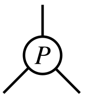
Figure 1: Left: The diagram for the interaction vertex $\sum_{i,j=1}^{R}\tilde{\Lambda}_{ij}P^{i}_{abc}\phi_{a}^{j}\phi_{b}^{j}\phi_{c}^{j}$. Right: The diagrams obtained by evaluating (28) through (29).

Through the replacement (29), (28) can be computed by the standard procedure using the Wick theorem and Feynman diagrams. A Wick contraction is performed by

$$\langle\phi_{a}^{i}\phi_{b}^{j}\rangle_{\phi}=\frac{1}{2\beta}\delta_{ab}\delta^{ij},$$ (31)

which can be derived by an explicit computation of (30). The Feynman diagram for the vertex $\sum_{i,j=1}^{R}\tilde{\Lambda}_{ij}P^{i}_{abc}\phi_{a}^{j}\phi_{b}^{j}\phi_{c}^{j}$ is shown in the left figure of Figure 1. Each leg is supposed to bring the two indices of $\phi_{a}^{i}$, and a Wick contraction connects two legs with the identification of their indices as in (31). A caution is that each leg on one vertex brings independent lower indices, but a common upper index.

Now let us apply the Wick contractions to what is obtained by replacing (28) with (29). We find the two diagrams shown in the right figure of Figure 1. Their degeneracy factors are 6 and 9, respectively, by counting the numbers of the ways to connect the legs of the two vertices. Since $j$ and $j^{\prime}$ in (28) are identified by the Wick contractions, we also get $\sum_{j=1}^{R}\tilde{\Lambda}_{ij}\tilde{\Lambda}_{i^{\prime}j}=\Lambda_{ii^{\prime}}$ as a factor (See (22).). Thus, we obtain

$$\langle(P\tilde{\phi}^{3})^{2}\rangle^{c}_{\tilde{\phi}}=\gamma_{3}\sum_{i,j=1}^{R}\Lambda_{ij}\left(6P^{i}_{abc}P^{j}_{abc}+9P^{i}_{aab}P^{j}_{bcc}\right),$$ (32)

where one notices that the factor $(2\beta)^{3}$ coming from the replacement (29) is exactly canceled by the factors of the three Wick contractions (31) performed for the evaluation. Putting the result (32) into (27), one obtains the effective action in the second order of $P_{abc}^{i}$ as

$$\begin{split}&S_{eff}^{(2)}(P)=\sum_{i,j=1}^{R}\left(\delta_{ij}P^{i}_{abc}P^{j}_{abc}+2\gamma_{3}\Lambda_{ij}t\left(6P^{i}_{abc}P^{j}_{abc}+9P^{i}_{aab}P^{j}_{bcc}\right)\right).\end{split}$$ (33)

The computation of (26) has now been reduced to diagonalizing the quadratic expression (33). The upper and lower indices can independently be diagonalized, because (33) has the form of the direct product with respect to these indices. More explicitly, since $\Lambda_{ij}$ is real and symmetric, we can consider the following decomposition into the eigenspaces:

$$\Lambda_{ij}=\sum_{\lambda_{ev}}\lambda_{ev}\,v^{\lambda_{ev}}_{i}v^{\lambda_{ev}}_{j},$$ (34)

where $v^{\lambda_{ev}}$ are the orthonormal eigenvectors, and the sum is over all the eigenvalues (with their degeneracies). By putting this and $\sum_{\lambda_{ev}}v^{\lambda_{ev}}_{i}v^{\lambda_{ev}}_{j}=\delta_{ij}$ into (33), we obtain a decomposition,

$$\begin{split}&S_{eff}^{(2)}(P)=\sum_{\lambda_{ev}}\left(P^{\lambda_{ev}}_{abc}P^{\lambda_{ev}}_{abc}+2\gamma_{3}\lambda_{ev}t\left(6P^{\lambda_{ev}}_{abc}P^{\lambda_{ev}}_{abc}+9P^{\lambda_{ev}}_{aab}P^{\lambda_{ev}}_{bcc}\right)\right),\end{split}$$ (35)

where $P^{\lambda_{ev}}_{abc}:=\sum_{i=1}^{R}v^{\lambda_{ev}}_{i}P^{i}_{abc}$.

Next let us diagonalize the lower index part in (35),

$$P_{abc}P_{abc}+2\gamma_{3}\lambda_{ev}\,t\left(6P_{abc}P_{abc}+9P_{aab}P_{bcc}\right),$$ (36)

where for brevity we omit $\lambda_{ev}$ from $P^{\lambda_{ev}}_{abc}$. Let us separate $P_{abc}$ into the tensor part $P^{T}_{abc}$ and the vector part $P^{V}_{abc}$, which are defined by

$$\begin{split}P_{abc}&=P^{T}_{abc}+P^{V}_{abc},\\ P^{V}_{abc}&=\frac{1}{N+2}\left(P_{add}\delta_{bc}+P_{bdd}\delta_{ca}+P_{cdd}\delta_{ab}\right).\end{split}$$ (37)

It is easy to check that $P^{T}_{abc}P^{V}_{abc}=0$ and $P^{V}_{abc}P^{V}_{abc}=\frac{3}{N+2}P_{abb}P_{acc}$. In particular, the former identity implies that $P^{T}_{abc}$ and $P^{V}_{abc}$ are independent degrees of freedom. Then, by using (37) and the identities above, (36) can be expressed as

$$(1+12\gamma_{3}\lambda_{ev}\,t)P^{T}_{abc}P^{T}_{abc}+\left(1+6(N+4)\gamma_{3}\lambda_{ev}\,t\right)P^{V}_{abc}P^{V}_{abc}.$$ (38)

The number of independent components contained in $P^{T}_{abc}$ and $P^{V}_{abc}$ are $\#P^{T}=N(N+1)(N+2)/6-N=N(N+4)(N-1)/6$ and $\#P^{V}=N$, respectively. Therefore, by putting this diagonal form into (26) and integrating over $P^{V}$ and $P^{T}$, we finally obtain the expression of $f_{N,R,\Lambda_{ij}}(t)$ from the quadratic order $S_{eff}^{(2)}(P)$ as

$$\begin{split}&f^{(2)}_{N,R,\Lambda_{ij}}(t)=const.\int dPe^{-S^{(2)}_{eff}(P)}\\ &\hskip 14.22636pt=\prod_{\lambda_{ev}}(1+12\gamma_{3}\lambda_{ev}t)^{-\frac{N(N+4)(N-1)}{12}}\left(1+6(N+4)\gamma_{3}\lambda_{ev}\,t\right)^{-\frac{N}{2}}\\ &\hskip 14.22636pt=\prod_{\lambda_{ev}}h_{N,R}(\lambda_{ev}t),\end{split}$$ (39)

where we have determined the overall factor by requiring $f^{(2)}_{N,R,\Lambda_{ij}}(0)=1$, the product is over all the eigenvalues of the matrix $\Lambda_{ij}$, and $h_{N,R}(x)$ is defined in (15).

For the computation of the observables discussed in Section 3, we consider $\Lambda_{ij}=\lambda+\lambda_{d}\delta_{ij}$. In this case, the matrix $\Lambda_{ij}$ has one eigenvalue $\lambda R+\lambda_{d}$ with the eigenvector $(1,1,\ldots,1)$, and the eigenvalue $\lambda_{d}$ with degeneracy $R-1$ with any of the vectors transverse to $(1,1,\ldots,1)$ as the eigenvectors. Therefore, from (39), we obtain

$$f^{(2)}_{N,R,\lambda+\lambda_{d}\delta_{ij}}(t)=h_{N,R}(\lambda Rt+\lambda_{d}t)\ h_{N,R}(\lambda_{d}t)^{R-1}.$$ (40)

This is the leading-order result shown in (14).

As we will see later in Section 6, there are some deviations between the leading-order result above and the numerical simulations. To see how the situation changes by adding some corrections, we have also computed the next-leading order. The details of the computation are given in Appendix D. The final result is

$$f^{next-leading}_{N,R,\lambda,\lambda_{d}}(t)=f^{leading}_{N,R,\lambda,\lambda_{d}}(t)\left(1-\langle S_{eff}^{(4)}(P)\rangle_{P}\right),$$ (41)

where $f^{next-leading}_{N,R,\lambda,\lambda_{d}}(t)$ is the sum of the leading and the next-leading orders, and

$$\begin{split}&\langle S_{eff}^{(4)}(P)\rangle_{P}\\ &=-\frac{4t^{2}}{4!}\Big{[}\gamma_{6}RG_{1}(x_{1},y_{1})-3(\gamma_{3}^{2}-\gamma_{6})\big{(}G_{2}(x_{2},y_{2})+(\lambda R+\lambda_{d})^{2}G_{3}(x_{3},y_{3})+(R-1)\lambda_{d}^{2}G_{3}(x_{4},y_{4})\big{)}\Big{]}\end{split}$$ (42)

with the definitions of $G_{i},x_{i},y_{i}$ given by from (109) to (119).

5 Saddle point analysis in the leading order

The integral expressions of the observables (18) in the leading order do not seem to have explicit expressions with known functions. Therefore, a way to obtain their explicit values is to numerically perform the integrations. This will be performed in Section 6 to compare with the Monte Carlo results. In this section, on the other hand, we will apply the saddle point approximation to the integrals to obtain a qualitative global picture of the phase structure of the model.

To discuss the saddle point approximation of the partition function (3), let us consider the minus of the logarithm of the integrand, which is given by

$$\begin{split}&{\cal F}_{N,R}(\lambda,k,r)\equiv f_{0}-(NR-1)\log r-\log f_{N,R}(\lambda r^{6})+kr^{2}.\end{split}$$ (43)

with $f_{0}=-\log V_{NR-1}$. A saddle point $r=r_{*}$ of the integral is determined by

$$\left.\frac{\partial}{\partial r}{\cal F}_{N,R}(\lambda,k,r)\right|_{r=r_{*}}=0$$ (44)

with the second derivative being positive at the point. As $f_{N,R}$, we take (5), which is the expression in the leading order of $1/R$:

$$\begin{split}&{\cal F}^{1/R,leading}_{N,R}(\lambda,k,r):=f_{0}-(NR-1)\log r+A_{0}\log(1+A_{1}r^{6})+B_{0}\log(1+B_{1}r^{6})+kr^{2}\end{split}$$ (45)

with

$$\begin{split}&A_{0}=\frac{N(N-1)(N+4)}{12},\ A_{1}=\frac{12\lambda}{N^{3}R^{2}},\\ &B_{0}=\frac{N}{2},\ B_{1}=\frac{6(N+4)\lambda}{N^{3}R^{2}}.\end{split}$$ (46)

In the saddle point approximation, the free energy of the model is approximated by

$$F^{free}_{N,R}(\lambda,k)\sim{\cal F}^{1/R,leading}_{N,R}(\lambda,k,r^{*})+\hbox{unimportant terms},$$ (47)

where the unimportant terms contain $\log V_{NR-1}$, which does not depend on $\lambda$ or $k$, and also some lower order terms in $N$, which will be discussed in the last paragraph of this section.

Let us first show that there exists a unique solution to the saddle point equation (44), for the leading order expression (45), in the integration region $r\geq 0$. To see this, it is convenient to use a new parametrization of $R$ in terms of $\alpha$ as $R=R_{c}(1+\alpha)$ with $R_{c}=(N+1)(N+2)/2$ and $-1<\alpha$. Then, by noting $NR_{c}=6(A_{0}+B_{0})$, the saddle point equation (44) with (45) can be written as

$$NR_{c}\alpha-1+\frac{6A_{0}}{1+A_{1}r_{*}^{6}}+\frac{6B_{0}}{1+B_{1}r_{*}^{6}}=2kr_{*}^{2}.$$ (48)

The lefthand side is obviously a decreasing function of $r_{*}$ with a maximum at $r_{*}=0$, while the righthand side is an increasing function from zero to the infinity. Since the maximum on the lefthand side is $NR_{c}\alpha-1+6A_{0}+6B_{0}=NR-1$, there always exists a unique solution of $r_{*}$ for $N,R\geq 1$. Moreover, the solution is smooth: $r_{*}$ does not jump in a discrete manner, when the parameters are continuously changed, because the $r_{*}$-dependence of each side continuously changes. This turns down the possibility that the model has a discontinuous phase transition in this treatment.

To discuss the solution more quantitatively with approximations, let us restrict ourselves to the parameter range of our interest: $\lambda\sim O(1)$, $N\gtrsim O(10)$, and $k\lesssim O(1)$. In addition, for the simplicity of the following discussions, let us avoid the region around $\alpha\sim 0$. By noting that $NR_{c},$ and $A_{0}$ are of order $O(10^{3})$ or larger, one can find that, for each case of $\alpha<0$ and $\alpha>0$, there are only two relevant terms among all in (48). For $\alpha<0$, the first and third terms on the lefthand side are relevant, and for $\alpha>0$, the first term on the lefthand side and the one on the righthand side are relevant. By solving the equations under taking these relevant terms only, the solutions are respectively given by

$$r_{*}^{2}\sim\left\{\begin{array}[]{ll}\left(\frac{1}{A_{1}}\left(-\frac{6A_{0}}{NR_{c}\alpha}-1\right)\right)^{\frac{1}{3}},&\alpha<0,\\ \frac{NR_{c}\alpha}{2k},&\alpha>0.\end{array}\right.$$ (51)

The first case shows divergent behavior for $\alpha\rightarrow-0$. However, this should not be taken as it is, since the transition should not have such an abrupt behavior as discussed above. In fact, the simplification taken above brakes down in the vicinity of $\alpha\sim 0$, and the real behavior is such that $r_{*}^{2}$ smoothly interpolates between the two parameter regions in the vicinity of $\alpha\sim 0$.

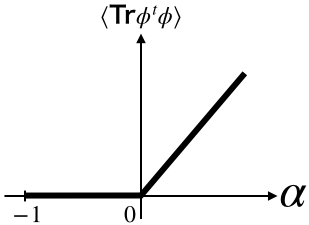
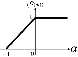
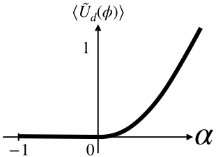
Figure 2: The behavior of the observables with respect to $\alpha=(R-R_{c})/R_{c}$ in the large $N$ limit, based on the saddle point analysis with the use of the leading order result of $f_{N,R}$. The parameters are assumed to be $\lambda\sim O(1)$ and $k\lesssim O(1)$.

The $r_{*}^{2}$ in (51) has different large-$N$ behavior in the two regions: $N^{\frac{7}{3}}$ for $\alpha<0$ and $N^{3}$ for $\alpha>0$. By normalizing $r_{*}^{2}$ with the common factor $(NR_{c})^{-1}$ for both the regions, we obtain

$$\tilde{r}_{*}^{2}\sim\left\{\begin{array}[]{cl}0,&\alpha\leq 0,\\ \frac{\alpha}{2k},&\alpha>0,\end{array}\right.$$ (54)

in the $N\rightarrow\infty$ limit, where $\tilde{r}_{*}^{2}:=(NR_{c})^{-1}r_{*}^{2}$. See the leftmost figure in Figure 2. This characterizes the transition at $\alpha=0$ as a continuous phase transition with $\langle\hbox{Tr}(\phi^{t}\phi)\rangle/(NR_{c})=0$ for $\alpha\leq 0$ and $\langle\hbox{Tr}(\phi^{t}\phi)\rangle/(NR_{c})=\frac{\alpha}{2k}$ for $\alpha>0$ in the thermodynamic limit.

The other observables can be treated in similar manners. By taking (18), putting $r=r_{*}$, and taking the leading order in large $N$, one obtains

$$\begin{split}\langle U(\phi)\rangle_{leading}&\sim\left\{\begin{array}[]{cl}\frac{N^{3}}{12\lambda}(1+\alpha),&\hbox{for }\alpha\leq 0,\\ \frac{N^{3}}{12\lambda},&\hbox{for }\alpha>0,\\ \end{array}\right.\\ \langle U_{d}(\phi)\rangle_{leading}&\sim\left\{\begin{array}[]{cl}\frac{N^{3}(1+\alpha)}{12\lambda(-\alpha)},&\hbox{for }\alpha\leq 0,\\ \frac{N^{5}}{16k^{3}}\frac{\alpha^{3}}{(1+\alpha)^{2}},&\hbox{for }\alpha>0.\end{array}\right.\end{split}$$ (55)

The divergence of $\langle U_{d}(\phi)\rangle_{leading}$ in $\alpha\rightarrow-0$ should not be taken as it is, because of the same reason mentioned above for $r_{*}^{2}$. By normalizing $\tilde{U}(\phi):=(N^{3}/12\lambda)^{-1}U(\phi)$ and $\tilde{U}_{d}(\phi):=(N^{5}/16k^{3})^{-1}U_{d}(\phi)$, one obtains

$$\begin{split}\langle\tilde{U}(\phi)\rangle_{leading}&\sim\left\{\begin{array}[]{cl}1+\alpha,&\hbox{for }\alpha\leq 0,\\ 1,&\hbox{for }\alpha>0,\\ \end{array}\right.\\ \langle\tilde{U}_{d}(\phi)\rangle_{leading}&\sim\left\{\begin{array}[]{cl}0,&\hbox{for }\alpha\leq 0,\\ \frac{\alpha^{3}}{(1+\alpha)^{2}},&\hbox{for }\alpha>0.\end{array}\right.\end{split}$$ (56)

See the middle and rightmost figures in Figure 2. The results support the same conclusion that there is a continuous phase transition at $\alpha=0$.

Let us finally comment on the consistency of the above saddle point approximation in the large $N$ case. From (45) and (51), it is straightforward by some explicit computations to find the expansion of ${\cal F}^{1/R,leading}_{N,R}$ around $r\sim r_{*}$ as

$${\cal F}^{1/R,leading}_{N,R}\sim a_{0}+a_{2}(r-r_{*})^{2}+a_{3}(r-r_{*})^{3}+\cdots,$$ (57)

where $a_{n}:=\frac{1}{n!}\frac{d}{dr^{n}}{\cal F}^{1/R,leading}_{N,R}(\lambda,k,r)|_{r=r_{*}}$ can easily be estimated as $a_{0}\sim O(N^{3})$, and

$$\begin{split}&a_{2}\sim O(N^{2/3}),\ a_{3}\sim O(N^{-1/2}),\hbox{ for }\alpha<0,\\ &a_{2}\sim O(1),\ a_{3}\sim O(N^{-3/2}),\hbox{ for }\alpha>0.\end{split}$$ (58)

Therefore the integral is dominated by the saddle point value $a_{0}$, and the Gaussian integration around the saddle point and the higher orders in $r-r^{*}$ are subdominant. In addition, the insertion of the observables ${\cal O}$ as in (18) for the computations of their expectation values does not change the location of the saddle point in the leading order, because the additional contribution $\log{\cal O}$ to (57) is $O(\log N)$, and cannot become comparable to the leading $O(N^{3})$ terms.

6 Comparison with Monte Carlo simulations

Figure 3: The numerical results of e.v. of the observables discussed in Section 3 for $\lambda=1$, $N=5$ and $k=0.1$ (top three) and $k=1.0$ (bottom three) against $R$. Plotted points represent the Monte Carlo results and ‘leading’ and ‘next-leading’ mean the evaluations based on Eq.(12) with perturbatively evaluated $f_{N,R,\lambda,\lambda_{d}}(t)$ in the leading and next-leading orders, respectively. There are some small windows within the figures, where one can see which of the leading and next-leading lines exists above/below the other, and can also see more clearly the results for $\langle U_{d}\rangle$ in the transition region around $R=R_{c}$. For the clarity of the small $R$ regions, which are unclear in some of the figures, we provide Figure 4.

Figure 4: Magnification of the small $R$ regions that are unclear in Figure 3.

Figure 5: $\lambda=1$, $N=10$ and $k=0.05$ (top three), $k=0.10$ (middle three) and $k=1.00$ (bottom three) against $R$. The same notations are used, and some small windows are put for the same purposes as in Figures 3. For the clarity of the small $R$ regions that are unclear in some of the figures, we provide Figure 6.

Figure 6: Magnification of the small $R$ regions that are unclear in Figure 5.

In Section 4, we have computed the leading order approximation of $f_{N,R,\lambda,\lambda_{d}}(t)$ defined in (11) in a perturbative method, and have obtained the result (14) along with (15) and so on. We have also derived the next-leading order correction (41) with (42), the details of which are given in Appendix D. With those results, we can numerically calculate the expectation values (e.v.) of the observables given in (12) by the expressions on the righthand sides. However, note that the above approximations of $f_{N,R,\lambda,\lambda_{d}}(t)$ are based on taking the perturbative expansion of $S_{eff}$ given in (27) up to the second order in $t$. Therefore they seem to require the implicit assumption of small values of $t$, and may not generally be trusted for the computation of (12), because $t$ is finally assigned with $r^{6}$, and $r$ is integrated over zero to infinity.

In view of the question above, it would be interesting to compute our model without any adoption of approximation methods. More specifically, in this section we compute the e.v. of the observables, (6) with ${\cal O}(\phi)=\hbox{Tr}(\phi^{t}\phi),U(\phi),U_{d}(\phi)$, by the Monte Carlo simulations, and compare them with the analytical results obtained by numerically integrating the righthand sides of (12), where we put our perturbative results for $f_{N,R,\lambda,\lambda_{d}}(t)$. Note that, in our strategy of the approximations, $R$ is not an expansion parameter, only $t$ is, and therefore it is meaningful to compare the results in the full range of $R$.

The results of the comparison are summarized in Figures 3, 4, 5 and 6. The points, each with an error bar (though it’s very small), represent the Monte Carlo results. For the information about the parameters taken in the Monte Carlo simulations, refer to the captions. In particular, we take $\lambda=1$ in all the computations, because $\lambda$ in the model (1) can be scaled out by a scale transformation $\phi\rightarrow\lambda^{-1/6}\phi$ so that it is absorbed into $k$ as $k/\lambda^{1/3}$. The dotted and chained lines represent the values of the e.v. of the observables in the leading and the next-leading orders by adopting $f_{N,R,\lambda,\lambda_{d}}(t)^{leading/next-leading}$ to (12), respectively. In some figures, it is difficult to distinguish these two lines, almost overlapping with each other. Therefore, we put some small windows within the figures, where these two lines can be distinguished, clearly showing which of them exists above/below the other. In fact, the relative locations (namely, above/below) of the two lines remain unchanged for each observable throughout the parameters $N,R$ and $k$ in the figures. In the small windows within the figures of $\langle U_{d}\rangle$, one can more clearly see the results in the vicinity of the transition region around $R=R_{c}$. In addition, for the clarity of the small $R$ regions of some of the figures, we provide Figures 4 and 6, where one can in particular find that the analytical and Monte Carlo results approach each other as $R$ becomes smaller.

An important thing that can be observed in the figures is that, for each $N$, there exists a region of $R$ that separates the smaller and larger regions of $R$ with different qualitative behaviors of the observables. This is more clearly seen for larger $N$ and smaller $k$. The transition region we observe indeed exists around the value $R_{c}=(N+1)(N+2)/2$, which was obtained as the critical point from the saddle point analysis in Section 5 (See Figure 2.).

It is an important physical question whether this transition of behavior is a phase-transition or just a crossover in the thermodynamic limit $N\rightarrow\infty$. However, we cannot currently answer this question for certain with the Monte Carlo results presently available, and this would require larger scale Monte Carlo simulations. It seems also difficult to answer this question by our perturbative analytical methods because of the following reason. In the figures, we can find good agreement between the perturbative computations and the Monte Carlo results in the regions away from the transition region. This would support the validity of our perturbative calculations in those outside regions. On the other hand, we can observe that there exist some deviations between the perturbative computations and the Monte Carlo results in the transition region. The deviations appear in such a way that the Monte Carlo results smoothen the transition to make it more like a crossover. Therefore, it seems that the analytical expressions we have obtained as approximations do not seem to be reliable in the transition region.

We can further discuss this complication from another view point as follows. Let us look at the figures more closely. Then we can find that, as to the numerical relations among $\langle\textrm{Tr}\phi^{t}\phi\rangle$, $\langle U\rangle$, and $\langle U_{d}\rangle$ in the leading and the next-leading orders, the following hold:

$$\begin{split}\langle\textrm{Tr}\,\phi^{t}\phi\rangle\,:&\textrm{ including next-leading $>$ leading},\\ \langle U\rangle\,:&\textrm{ including next-leading $<$ leading},\\ \langle U_{d}\rangle\,:&\textrm{ including next-leading $<$ leading},\end{split}$$ (59)

for all $R$. Therefore, while the next-leading order corrections indeed improve the approximations so that they approach the Monte Carlo results in the outside regions and this is also so for $\langle\textrm{Tr}\,\phi^{t}\phi\rangle$ and $\langle U\rangle$ in the transition region, the last inequality about $\langle U_{d}\rangle$ is in the opposite direction. This suggests that our perturbative treatment seems to have some difficulties in correctly taking into account some configurations that mainly contribute to $U_{d}$ in the transition region. It would be an interesting future problem to identify these configurations.

Let us briefly explain our actual Monte Carlo simulations. We have performed Monte Carlo simulations with the standard Metropolis update method for the model (1) by using KEKCC, the cluster system of KEK. For each calculation shown in the figures, we performed 2 billion sweeps, where the time taken for this was generally about 7 and 23 hours with $R=10$ and $130$, respectively. We stored the data of the observables once per 400 sweeps, and computed their mean values and the $1\sigma$-errors by the Jackknife resampling method. In each calculation we always set the acceptance rate to be around 60$\%$. However, to realize this 60$\%$, we had to tune the step sizes in our Metropolis method to quite small values, especially in the region $R\gtrsim N^{2}/2$.

Let us further comment on the last peculiar nature we encountered in the simulations. We have performed the simulations for $k=1,0.1$ and $0.05$ with $N=10$ and $k=1.0$ and $0.1$ with $N=5$, respectively, as shown in the figures. As suggested by the results in the figures, the transition could be sharpened, if we performed simulations with smaller values of $k$ than those in the figures. However, when we tried to do so, we encountered a serious difficulty in particular in the region $R\gtrsim N^{2}/2$. It was that the Metropolis step sizes must be tuned to very small values to keep the reasonable acceptance rate like 60%. Then, the performance of the simulations became so slow that we could not find the timing when the system had reached thermodynamic equilibriums: The system always looked like being in the middle stage of moving very slowly toward thermodynamic equilibriums, at least during one week of continuous running or so. Therefore we took relatively large values of $k$ as those in the figures to avoid the serious difficulty that makes the simulations unreliable.

Finally, let us qualitatively explain why the analytical results computed by the perturbative method and the Monte Carlo results agree with each other outside the transition region of $R$. Let us start with a qualitative estimation of the effective action (27) with respect to the orders in $R$ and $t$. One can obtain

$$S_{eff}(P)\sim(1+b_{0}\,t)P^{2}+b_{1}\,t^{2}P^{4}+\cdots,$$ (60)

where we have ignored all the index structures of $P^{i}_{abc}$ for notational simplicity, and the dominant $R$-dependencies of the coefficients are given by

$$\begin{split}b_{0}\sim\frac{c_{0}}{R^{2}},\ b_{1}\sim\frac{c_{1}}{R^{5}}.\end{split}$$ (61)

Here the dominant $R$-dependence of $b_{0}$ is obtained by putting the eigenvalue $\lambda_{ev}\sim R$ into (36) and recalling $\gamma_{3}\sim 1/R^{3}$, as defined in (16); The estimation of $b_{1}$ is also straightforward and is given in Appendix E. Then, normalizing the quadratic part by rescaling $P\rightarrow P/\sqrt{1+b_{0}t}$ in (60), one finds that the actual quartic coupling of $S_{eff}$ is estimated as

$$\frac{b_{1}\,t^{2}}{(1+b_{0}t)^{2}}\sim\frac{c_{1}t^{2}}{R(R^{2}+c_{0}t)^{2}},$$ (62)

which is different from the naive value $b_{1}\,t^{2}$. When $R$ is small, $r^{2}={\rm Tr}(\phi^{t}\phi)$ is dominated by small values as shown in the Monte Carlo computations above. This means that, since $t\sim r^{6}$ in the usage (3), (62) is also dominated by small values, and therefor the quadratic term $S_{eff}^{(2)}$ will give good analytic estimations. On the other hand, when $R$ is large, $t\sim r^{6}$ is dominated by large values as shown in the Monte Carlo results. Nonetheless what is remarkable is that (62) is always suppressed by $1/R$ irrespective of the values of $t$. Therefore the leading order term $S_{eff}^{(2)}$ will again give good estimations. In the middle region, however, (62) could generally become large, and higher order and/or non-perturbative corrections may substantially contribute, as suggested by the deviations between the Monte Carlo and analytical results.

7 Topological structure of configurations

In this section, we will explain our observation on the topological structure of the configurations generated by the Monte Carlo simulations. Topology of a value of the matrix $\phi_{a}^{i}$ can be analyzed by persistent homology [30], which is a modern technique of the topological data analysis (See Appendix F for a brief introduction of persistent homology.). More specifically, we performed the Monte Carlo simulations for $N=4$ and $R=10,15,20,25$ with $\lambda=1,\ k=0.01$, and, for each case, uniformly took 100 samples of the values of $\phi_{a}^{i}$ during a large number of sequential updates of order $10^{8}$ after thermodynamic equilibriums were seen to be reached. Then, the samples were analyzed in terms of persistent homology. The analysis shows that the favored topology of the configurations is $S^{1}$ for $R=10,15$, but gradually changes to higher dimensional cycles, when $R$ is increased. We will first explain the background motivation for this analysis, and will then show the results.

One of the present authors and his collaborators have been studying a tensor model in the canonical formalism, which we call canonical tensor model [16, 17], as a model of quantum gravity. In [18], it has been shown that the exact wave function of the tensor model has peaks at the configurations that are invariant under Lie groups. This phenomenon, which we call symmetry highlighting phenomenon, potentially has an important physical significance, since this phenomenon would imply the dominance of spacetimes symmetric under Lie groups through the correspondence between tensors and spaces developed in [19]. This symmetry highlighting phenomenon has first been shown for a toy wave function [20], which slightly simplifies the wave function of the canonical tensor model. The toy wave function is given by

$$\tilde{\varphi}(P)=\int_{\mathbb{R}^{N}}\prod_{a=1}^{N}d\phi_{a}\exp\left(IP_{abc}\phi_{a}\phi_{b}\phi_{c}+\left(I\kappa-\epsilon\right)\phi_{a}\phi_{a}\right),$$ (63)

where $I$ denotes the imaginary unit, and $\epsilon$ is a small positive regularization parameter to assure the convergence of the integral. The symmetry highlighting phenomenon is that the wave function has large peaks at $P_{abc}$ that are invariant under Lie groups: $P_{abc}=h_{a}^{a^{\prime}}h_{b}^{b^{\prime}}h_{c}^{c^{\prime}}P_{a^{\prime}b^{\prime}c^{\prime}}$ under ${}^{\forall}h\in H$, where $H$ is a representation of a Lie group. The phenomenon can qualitatively be understood by the following rough argument: If $P_{abc}$ is invariant under a Lie group, the integration over $\phi_{a}$ in (63) will contribute coherently along the gauge orbit $h_{a}^{a^{\prime}}\phi_{a^{\prime}}\ (^{\forall}h\in H)$, but, if this is not so, the contributions tend to cancel among themselves due to the phase oscillations of the integrand and the wave function takes relatively small values. In [20], some tractable simple cases have explicitly been studied, and the presence of the phenomenon has indeed be shown.

Other than the simple case studies, the peak structure of the toy wave function and that of the tensor model are largely unknown. One reason is that the number of independent components of $P_{abc}$, which is about $\sim N^{3}/6$, is so large that it is practically not possible to go over the whole configuration space of $P_{abc}$. Rather, we will be able to obtain rough knowledge by integrating over $P_{abc}$:

$$\begin{split}&\int_{-\infty}^{\infty}\prod_{a\leq b\leq c=1}^{N}dP_{abc}\ \tilde{\varphi}(P)^{R}\exp\left(-\alpha P_{abc}P_{abc}\right)={\rm const.}\,Z_{N,R}\left(\frac{1}{4\alpha},k\right),\end{split}$$ (64)

where we have denoted $k=-I\kappa+\epsilon$, and we have considered an arbitrary power $R$ of the wave function, because the actual wave function of the tensor model has the corresponding power which specifically takes $R=(N+2)(N+3)/2$ [18, 15, 29] (See Appendix A.). In (64), we see that the integration of a power of the wave function over $P_{abc}$ with a Gaussian weight produces the matrix model (1). If the integration is dominated by such peaks associated to Lie groups, we can expect that the $N$-dimensional vectors, $\phi_{a}^{i}\ (i=1,2,\ldots,R)$, in the matrix model tend to exist along some gauge orbits in the vector space.

In general, there exist a number of peaks (or rather ridges) associated with various Lie group symmetries and gauge orbits for the wave function (63). As argued and shown explicitly in [20, 18], peaks associated with lower dimensional Lie group symmetries generally exist more abundantly than those with higher dimensional symmetries, because the number of symmetry conditions that must be satisfied by $P_{abc}$ is smaller for the former than for the latter. On the contrary, the peaks of the latter are generally higher than those of the former, because the gauge orbits of the latter have larger dimensions and provide more coherent contributions than the former. Therefore, there are competitions between height and abundancy, and it is generally a subtle question which of lower or higher dimensional Lie group symmetries is probabilistically favored in a given case.

Let us discuss this question in view of the correspondence to the matrix model (64), especially by considering changing the value of $R$. As $R$ is the power of the wave function as in (64), larger $R$ will enhance higher peaks compared to the lower ones. Therefore we expect that, for larger $R$, the contributions from peaks with higher dimensional symmetries will be more dominant. Otherwise, peaks with lower dimensional Lie group symmetries will dominate because of their abundant existence. In addition, when $R$ is very small, non-symmetric configurations will dominate, since they exist most abundantly.

In the Monte Carlo simulation of our model, if a symmetric peak dominates as explained above, the $N$-dimensional vectors $\phi_{a}^{i}\ (i=1,2,\ldots,R)$ will be randomly distributed along the associated gauge orbit. A caution here is that the gauge orbit can take any $O(N)$-transformed location in the $N$-dimensional vector space due to the $O(N)$ symmetry of the model. Therefore we should not simply plot all the samples of $\phi_{a}^{i}$ generated by the Monte Carlo simulations in the $N$-dimensional vector space, since this will merely provide a trivial $O(N)$-invariant spherical distribution of points without any characteristics of the Lie-group symmetry associated to the dominant peak. Rather, we have to analyze each sample of $\phi_{a}^{i}$ generated by the Monte Carlo simulations to extract its characteristics, and then pile up all the extractions over all the samples to find allover characteristic properties.

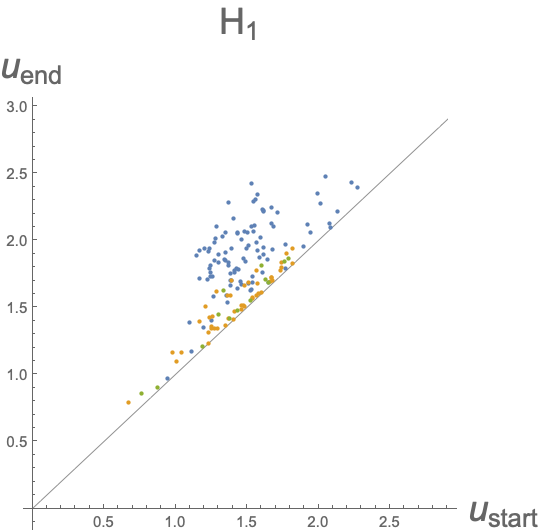
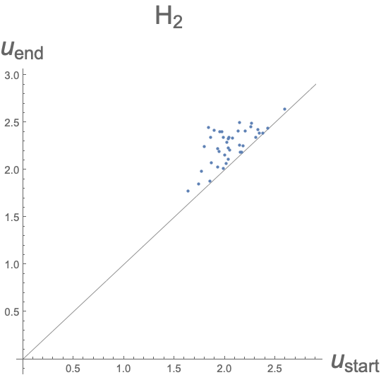
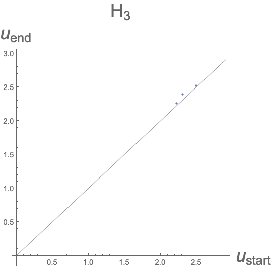
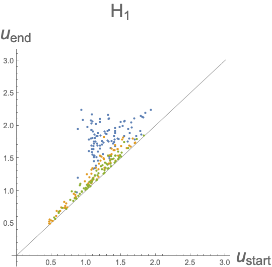
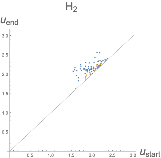
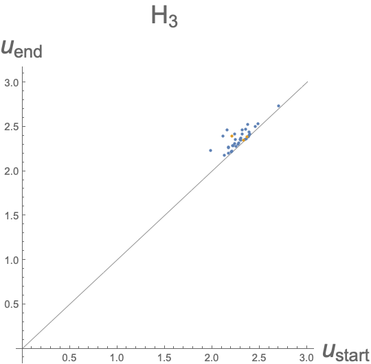
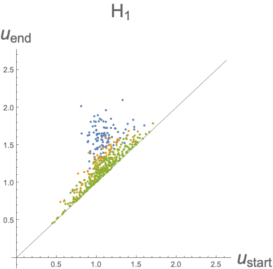
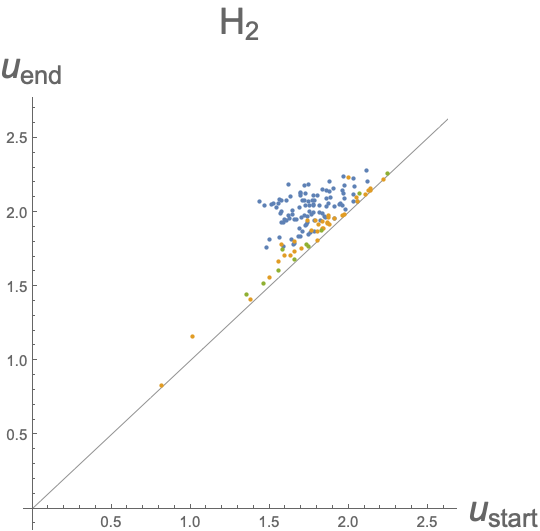
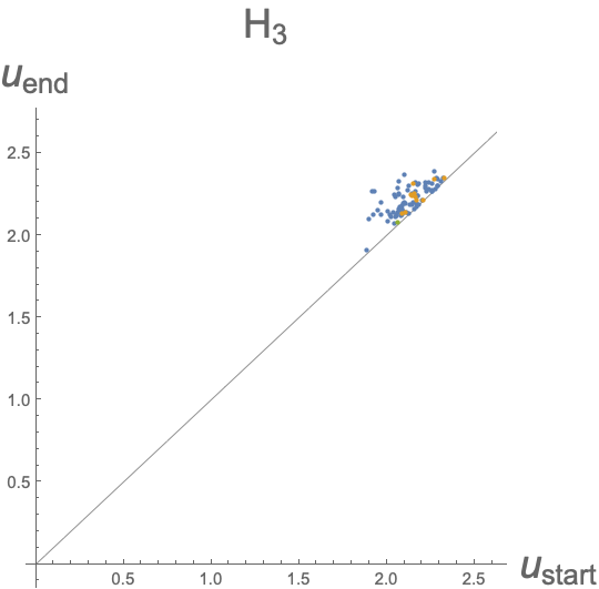
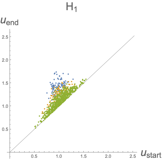
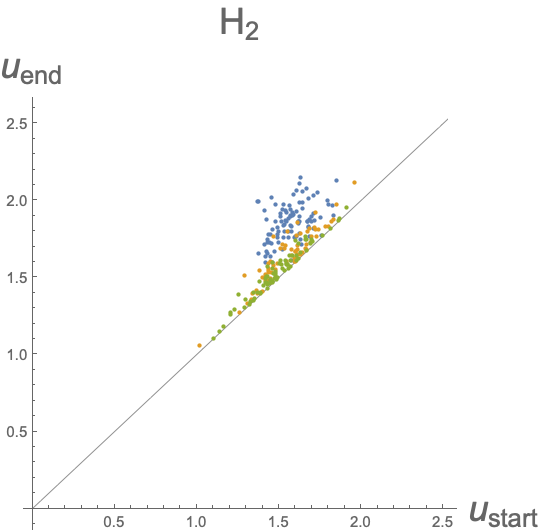
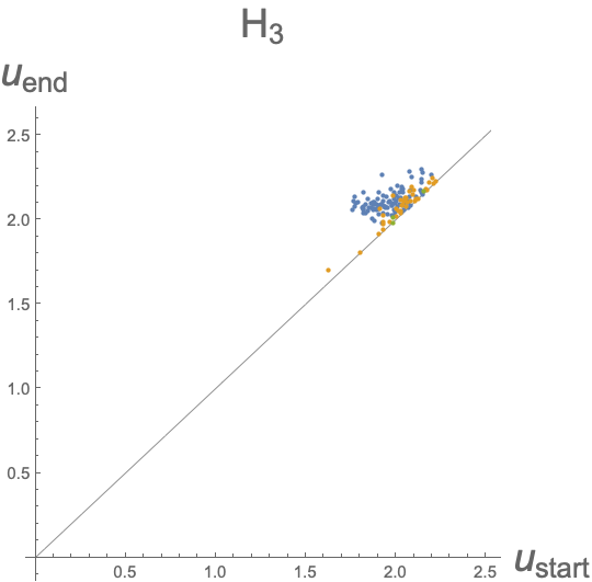
Figure 7: Persistent diagrams obtained from the Monte Carlo data of $N=4,\ k=0.01,\ \lambda=1$ with $R=10,15,20,25$ (from the top to the bottom). To avoid the dependence of the initial values, 10 independent Monte Carlo sequences were run, and the sampling were performed uniformly from the sequence of updates of $\sim 10^{9}$ after thermodynamic equilibriums were seen. 100 configurations of $\phi_{a}^{i}$ were uniformly sampled and the persistent homologies were analyzed (one- to three-dimensional homologies from the left to the right). The results of 100 samples are plotted on the same persistent diagrams. Blue dots represent the longest-life elements in each dimensional persistent homology group of each data, the yellow ones the second, and the green ones all after the second. The dots away from the diagonal line represent long-life persistent homology group elements, which are considered to be characteristics of a data, while those near the diagonal line are regarded as “noises”. The highest blue dots, namely those with the largest $u_{\rm end}$ that represent the largest structure, move from $H_{1}$ to $H_{2}$ and then $H_{3}$ with the increase of $R$.

Topological structure of each sample of $\phi_{a}^{i}$ can be analyzed by using the technique of persistent homology [30]. This is a modern applied mathematical technique of the topological data analysis, and can extract homology groups of a data (See Appendix F.). Here an input data should be a set of points with relative distances. We used an open-source c++ program that is called Ripser for the analysis and plotted the output with Mathematica. For a configuration $\phi_{a}^{i}$, we consider the replica number $i=1,2,\ldots,R$ to represent the label of “points” of a data set, and define the distances between two points $i$ and $j$ as

$$d(i,j):=\arccos\left(\frac{\phi_{a}^{i}\phi_{a}^{j}}{\sqrt{\phi_{a}^{i}\phi_{a}^{i}\phi_{b}^{j}\phi_{b}^{j}}}\right).$$ (65)

The gist of this definition is that the $N$-dimensional vectors $\phi_{a}^{i}\ (i=1,2,\ldots,R)$ are projected onto the unit sphere $S^{N-1}$, and the geodesic distances along the sphere are regarded as the distances. In particular, this definition is suited for detecting a gauge orbit $h_{a}^{b}\phi_{b}\ (h\in H)$, since it is projected on the sphere irrespective of the size of the vector $\phi_{a}$.

We want to see the phenomenon explained above in the actual Monte Carlo simulations. For this initial study, choosing small $N$ would be preferred for simper analysis, because then there exist a small number of possibilities of gauge orbits with small dimensions, and also thermodynamic equilibriums can easily be reached due to the small number of degrees of freedom. Note however that this trades off the clarity of the homology structure being detected by persistent homology. This is because, for small $N$, the values of $R$ at which the phenomenon appears are also rather small in the order of $R\sim N^{2}/2$, as we will see in the analysis below. The homology cycles formed by small numbers (namely $R$) of points necessarily become obscure, especially higher dimensional cycles are difficult to be clearly detected.

For the actual simulation, we considered $N=4$. In $N=4$, as explicitly solved in [20], there exist only two possibilities of Lie group symmetries, $SO(2)$ and $SO(3)$, and the gauge orbits are $S^{1}$ and $S^{2}$, respectively. In fact, the ridges of the $P_{abc}$ with these symmetries reach the origin $P_{abc}=0$, and therefore we should also add the trivial possibility of $S^{3}$ with the $SO(4)$ symmetry, which is the symmetry of $P_{abc}=0$ and is maximal. Figure 7 shows the persistent diagrams obtained from the Monte Carlo simulations with $R=10,15,20,25$. Statistically speaking, one can observe that, starting from $S^{1}$ at $R=10,15$, higher dimensional cycles gradually appear and become the largest structure when $R$ is increased, while lower dimensional cycles gradually take smaller values of $u$.

8 Summary and future prospects

In this paper, we studied a matrix model containing non-pairwise index contractions [21], which has a motivation from a tensor model of quantum gravity [16, 17]. More specifically, it has $\phi_{a}^{i}\ (a=1,2,\ldots,N,\ i=1,2,\ldots,R)$ as its degrees of freedom, where the lower indices are pairwise contracted, but the latter are not always done so. This matrix model has the same form as what appears in the replica trick of the spherical $p$-spin model for spin glasses [27, 28], though the variable and parameter ranges of our interest are different. We performed Monte Carlo simulations with the Metropolis update method, and compared the results with some analytical computations in the leading order, mostly based on the previous treatment in [21]. They are in good agreement outside the transition region, that is located around $R\sim N^{2}/2$. In the transition region, however, there exist deviations between the simulations and the analytical results, and the deviations cannot be corrected well, even if the next-leading order contributions are included. It has not been determined whether the transition is a phase transition or a crossover in the thermodynamic limit $N\rightarrow\infty$, because of the limited range of the parameters like $N\lesssim 10$ available in our Monte Carlo simulation. Our Monte Carlo simulation tended to slow down especially at $R\gtrsim N^{2}/2$ with large $\lambda/k^{3}$, suspecting that the system gets glassy nature in the region, but no conclusive argument has been made for this aspect. We also studied the topological characteristics of the configurations $\phi_{a}^{i}$ generated in the Monte Carlo simulations by using the modern technique called persistent homology [30] in topological data analysis. This technique extracts the homology structure of a data, which is a configuration of $\phi_{a}^{i}$ in our case. We observed that, in the vicinity of the transition region, the homology structure of the configurations gradually changes from $S^{1}$ to higher-dimensional cycles with the increase of $R$.

A particularly interesting result of this paper is that there seems to exist a transition region around $R\sim N^{2}/2$. Intriguingly, this value of $R$ coincides with what is required by the consistency of the tensor model (namely, the hermiticity of the hamiltonian constraint. See Appendix A.) [18, 15, 29]. Moreover, our model seems to have the most interesting properties in this region, but they are not well understood: There are some deviations between the simulation and the analytical results in this region, but the reason is not clear; The transition of the homological structure of the dominant configurations in this vicinity is peculiar but not well understood; Whether the transition is a phase transition or a crossover in the thermodynamic limit $N\rightarrow\infty$ is not determined. For the better understanding in the future, it seems necessary to treat larger $N$ cases with large $\lambda/k^{3}$ by employing more efficient methods of Monte Carlo simulations and finding more powerful analytical methods.

Appendices

Appendix Appendix A The motivation for the model (1) from the viewpoint of the canonical tensor model

In this appendix, we explain the motivation for the model (1) by summarizing the developments of the canonical tensor model so far.

An interesting direction in the attempt to formulate quantum gravity is to pursue the existence of the spacetime as an emergent phenomenon. In this context, the matrix models have achieved great success in the description of the two-dimensional quantum gravity [31]. To extend the success to higher dimensions, the tensor models [11, 12, 13, 14] were proposed as generalization of the matrix models. Though various interesting results have been obtained, emergence of spacetimes has not been achieved so far by these tensor models, suffering from the dominance of singular configurations instead of macroscopic space-like ones. Moreover, in these tensor models under the interpretation employed in these original papers [11, 12, 13, 14], the numbers of the indices of the tensorial dynamical variables have direct connections to the dimensions of the spaces supposed to be emergent. This is a drawback from the viewpoint of quantum gravity, since the number of dimensions should also be dynamically determined rather than predetermined as an input.

This drawback may be overcome by introducing a new interpretation of the tensor models. In fact, tensors themselves have rich structures enough to describe spaces. This can be seen by supposing that a three-index tensor, say $C_{ab}{}^{c}$, define the structure constants of an algebra of functions, say $f_{a}$, over a space by $f_{a}f_{b}=C_{ab}{}^{c}f_{c}$. It is known that spaces can be defined by the algebras of functions on them satisfying certain properties (see for example [32].). Though such algebras for usual spaces are commutative and associative, we would be able to suppose that more general $C_{ab}{}^{c}$, which defines noncommutative or/and nonassociative algebras, would define “fuzzy spaces”. This idea is explored to propose a new interpretation of three-index tensor models as models of dynamical fuzzy spaces [33]. Under this new interpretation, a three-index tensor model can in principle generate various dimensional spaces, not being restricted to certain dimensions [33]. One can also see the emergence of Euclidean general relativity on them [34, 35, 36, 37].

However, these favorable results were obtained only by doing some fine-tunings to the models [34, 35, 36, 37]. Moreover, time is missing in these tensor models. In fact, time might play essentially important roles in the mechanism of emergence of spacetime, as the success of the causal dynamical triangulation [2] shows over the dynamical triangulation. Generally speaking, introducing time requires delicate treatment in quantum gravity, since such models must respect the spacetime diffeomorphism invariance on emergent spacetimes. To introduce time with this delicate requirement, a tensor model, which we call the canonical tensor model (CTM), has been formulated as a constrained system in the Hamilton formalism [16, 17]. The model is composed of a number of first-class constraints analogous to those in the ADM formalism of general relativity. Therefore, CTM embodies an analogue of the spacetime diffeomorphism as its gauge symmetry. CTM is supposed to describe time-evolutions of fuzzy spaces.

The classical aspects of CTM have been compared with GR in a formal continuum limit with $N\rightarrow\infty$: The constraint algebra of CTM has been shown to agree with that of the ADM formalism of GR [38]; the classical equation of motion of CTM has been shown to agree with that of GR in the Hamilton-Jacobi formalism with a certain Hamilton’s principal function [39]. Simple cases with large but finite $N$ have also been studied, and mutual agreement has been obtained [19].

The canonical quantization of CTM is straightforward [29]. The classical constraints are transformed to the quantized ones with one additional term coming from operator ordering. The algebra essentially remains the same form, especially implying the closure of the commutation algebra among the quantized constraints. This assures the consistency of the physical state conditions given by

$$\hat{\cal H}_{a}|\Psi_{phys}\rangle=\hat{\cal J}_{ab}|\Psi_{phys}\rangle=0,$$ (66)

where $\hat{\cal H}_{a}$ and $\hat{\cal J}_{ab}$ denote the quantized constraints of CTM, respectively corresponding to the Hamiltonian and momentum constraints of ADM. By taking a certain representation, these equations become a system of partial differential equations for physical wave functions. At first sight they looked too complicated to solve, but it has turned out that there exist various explicit exact solutions to these equations [15]. In particular, a systematic solution is given in the $P$-representation by [15, 18]

$$\Psi(P)_{phys}=\varphi(P)^{\lambda_{H}/2},$$ (67)

where $\lambda_{H}=(N+2)(N+3)/2$, and

$$\varphi(P)=\int_{\mathbb{R}^{N+1}}d\tilde{\phi}\prod_{a=1}^{N}d\phi_{a}\,e^{I(P\phi^{3}-\phi^{2}\tilde{\phi}+\frac{4}{27\lambda}\tilde{\phi}^{3})}$$ (68)

with $P\phi^{3}\equiv P_{abc}\phi_{a}\phi_{b}\phi_{c}$, $\phi^{2}\equiv\phi_{a}\phi_{a}$, and $\lambda$ is an arbitrary real parameter, which can be normalized as $0,\pm 1$. The above value of $\lambda_{H}$ is uniquely determined by the hermiticity of the “Hamilotonian constraints” $\hat{\cal H}_{a}$ of CTM.

In principle, emergence of spacetime can be analyzed by investigating the properties of the wave function $\Psi(P)_{phys}$. The ideal situation would be that, in the configuration space, the quantum probability density $|\Psi(P)_{phys}|^{2}$ form some ridges that can be considered to be trajectories of classical time-evolutions of spaces. In fact, it has been qualitatively argued and actually been found in some tractable simple cases that such ridges exist at $P_{abc}$’s that are invariant under Lie-groups. Since symmetries are ubiquitous in the actual spacetimes, this result is encouraging in the pursuit for spacetime emergence. However, further analysis of $\Psi(P)_{phys}$ is not easy, and most of the properties of the wave function are still unknown. Therefore, it is presently not possible to discuss emergent spacetimes in CTM.

Yet, aiming for better understanding of $\Psi(P)_{phys}$, we consider in this paper a model which can be obtained after two simplifications. One is to integrate the quantum probability density over the configuration space:

$$\int_{\mathbb{R}^{\#P}}dP\,e^{-\alpha P^{2}}|\Psi(P)_{phys}|^{2},$$ (69)

where $dP\equiv\prod_{a\leq b\leq c}^{N}dP_{abc}$, $P^{2}\equiv P_{abc}P_{abc}$ and $\alpha$ is an arbitrary positive number. The other is to fix (or ignore) the integration variable $\tilde{\phi}$ of $\varphi(P)$ in (68) so that $\tilde{\varphi}(P)$ in (63) is used as $\varphi(P)$ in (67). The wave function after this replacement is still interesting enough, because $\tilde{\varphi}(P)$ has the similar connection between Lie-group symmetries and peaks [20]. Then, by putting $\tilde{\varphi}(P)$ into (67) and performing the Gaussian integration over $P$ in (69), one obtains

$$\int_{\mathbb{R}^{\#P}}dPe^{-\alpha P^{2}}\tilde{\varphi}(P)^{\lambda_{H}}=const.Z_{N,\lambda_{H}}\left(\frac{1}{4\alpha},k\right),$$ (70)

where we have used the reality of the wave function $\tilde{\varphi}(P)$ for the real value of $k=-I\kappa+\epsilon$. Here we have actually obtained the partition function $Z$ in (1) of the matrix model with the particular choice $R=\lambda_{H}\ (=(N+2)(N+3)/2)$. Since $\lambda_{H}\sim R_{c}\ (=(N+1)(N+2)/2)$, CTM seems to be located in the transition region of the matrix model.

Appendix Appendix B $R=2$ case

In this appendix, we consider the partition function for $R=2$, and see that the partition function is finite even for $k=0$. This is not trivial, because, for general $R>1$, the solution to $U(\phi)=0$ is non-empty (see below), and therefore there is a potential risk of runaway behavior, $\phi^{2}\rightarrow\infty$ with $U(\phi)=0$.

Let us first see that $U(\phi)=0$ is non-empty for general $R>1$. Since

$$U(\phi)=\left(\sum_{i=1}^{R}\phi^{i}_{a}\phi^{i}_{b}\phi^{i}_{c}\right)\left(\sum_{j=1}^{R}\phi^{j}_{a}\phi^{j}_{b}\phi^{j}_{c}\right),$$ (71)

$U(\phi)\geq 0$ holds, and $U(\phi)$ vanishes iff

$$\sum_{i=1}^{R}\phi^{i}_{a}\phi^{i}_{b}\phi^{i}_{c}=0.$$ (72)

An obvious set of solutions are given by $\phi_{a}^{2i-1}=-\phi_{a}^{2i},\ (i=1,2,\lfloor R/2\rfloor)$ with $\phi^{R}_{a}=0$ if $R$=odd.

For $R=2$, one can see that this is the only solution as follows. By contracting the indices $b$ and $c$ in (72), we obtain

$$\phi^{1}_{a}\phi^{1}_{b}\phi^{1}_{b}+\phi^{2}_{a}\phi^{2}_{b}\phi^{2}_{b}=0.$$ (73)

This implies that $\phi^{1}$ and $\phi^{2}$ are linearly dependent, and putting this back to (72), we obtain $\phi_{a}^{1}=-\phi^{2}_{a}$.

In the $R=2$ case, since $U(\phi)$ depends only on the relative directions and the sizes of $\phi_{a}^{1}$ and $\phi_{a}^{2}$, the partition function for $k=0$ can be written as

$$\begin{split}&Z_{N,R=2}(\lambda,k=0)=\hbox{Vol}(S^{N-1})\hbox{Vol}(S^{N-2})\int_{0}^{\infty}dr_{1}dr_{2}\ r_{1}^{N-1}r_{2}^{N-1}\int_{0}^{\pi}d\theta\sin^{N-2}(\theta)\ e^{-\lambda U(\theta)},\end{split}$$ (74)

where

$$U(r_{1},r_{2},\theta)=r_{1}^{6}+r_{2}^{6}+2r_{1}^{3}r_{2}^{3}\cos^{3}(\theta)$$ (75)

with $r_{1}$ and $r_{2}$ being the sizes, and $\theta$ being the relative angle. As shown above, the only case with $U=0$ is given by $r_{1}=r_{2},\ \theta=\pi$. Therefore let us perform the reparameterization,

$$r_{1}=r,\ r_{2}=r(1+x),\ \theta=\pi-y.$$ (76)

Then the integral of (74) at large $r$ can be approximated by expanding the integrand for small $x,y$, and we obtain

$$\sim\int drdxdy\ r^{2N-1}y^{N-2}e^{-3\lambda r^{6}(3x^{2}+y^{2})}\sim\int dr\ r^{-N-1}.$$ (77)

This shows that the partition function is convergent for $R=2$ and $k=0$.

There are two things which can be learned from this simplest case. One is that, if $R$ is small enough, the partition function is convergent even for $k=0$. Another thing is that the large-$r$ asymptotic behavior of the integrand is much slower than the leading order result,

$$\int drr^{NR-1}f^{leading}_{N,R}(\lambda r^{6})\sim\int dr\,r^{2N-1-N(N+1)(N+2)/2}.$$ (78)

Therefore the asymptotic behavior derived from the leading order result cannot be correct down to $R=2$.

Appendix Appendix C Derivation of (29)

In this section, we derive (29). This was previously derived in [21], but this is repeated here to make the present paper self-contained.

For $m=$odd, the equation holds, because the both sides vanish.

Let us assume $m=2p$ with a positive integer $p$. Let us start with the following equation:

$$\begin{split}&\frac{1}{\int_{S^{NR-1}}d\tilde{\phi}}\int_{S^{NR-1}}d\tilde{\phi}\,\tilde{\phi}_{a_{1}}^{i_{1}}\tilde{\phi}_{a_{2}}^{i_{2}}\cdots\tilde{\phi}_{a_{2p}}^{i_{2p}}=\frac{1}{\int_{{\mathbb{R}}^{NR}}d\phi\ e^{-\beta{\rm Tr}\phi^{t}\phi}}\int_{{\mathbb{R}}^{NR}}d\phi\ \frac{\phi_{a_{1}}^{i_{1}}\phi_{a_{2}}^{i_{2}}\cdots\phi_{a_{2p}}^{i_{2p}}}{({\rm Tr}\phi^{t}\phi)^{p}}e^{-\beta\,{\rm Tr}\phi^{t}\phi},\end{split}$$ (79)

where $\beta$ is an arbitrary positive constant. This can easily be proven by reparameterizing $\phi_{a}^{i}$ with the radial and the angular variables as $\phi_{a}^{i}=r\tilde{\phi}_{a}^{i}$ on the righthand side, and observing that the integrations over $r$ decouples from the angular part and cancels between the numerator and the denominator.

Let us consider the numerator on the righthand side of (79),

$$A(\beta):=\int_{{\mathbb{R}}^{NR}}d\phi\ \frac{\phi_{a_{1}}^{i_{1}}\phi_{a_{2}}^{i_{2}}\cdots\phi_{a_{2p}}^{i_{2p}}}{({\rm Tr}\phi^{t}\phi)^{p}}e^{-\beta{\rm Tr}\phi^{t}\phi}.$$ (80)

Taking the $p$-th derivative of $A(\beta)$ with respect to $\beta$ cancels the $({\rm Tr}\phi^{t}\phi)^{p}$ in the denominator of the inetegrand. On the other hand, by performing the rescaling $\phi_{a}^{i}\rightarrow\beta^{-1/2}\phi_{a}^{i}$, it is obvious that $A(\beta)$ has the dependence $\beta^{-NR/2}$ on $\beta$. Therefore, by performing the $p$-th derivative of the both sides of (80), we obtain the relation,

$$\frac{\Gamma\left(\frac{NR}{2}+p\right)}{\Gamma\left(\frac{NR}{2}\right)}\beta^{-p}A(\beta)=\int_{{\mathbb{R}}^{NR}}d\phi\ \phi_{a_{1}}^{i_{1}}\phi_{a_{2}}^{i_{2}}\cdots\phi_{a_{2p}}^{i_{2p}}e^{-\beta\,{\rm Tr}\phi^{t}\phi}.$$ (81)

By solving for $A(\beta)$ and putting it into (79), we obtain (29).

Appendix Appendix D Computation of $f_{N,R,\Lambda_{ij}}(t)$ in the next-leading order

In this appendix, we will compute the fourth-order term $\langle(P\tilde{\phi}^{3})^{4}\rangle_{\tilde{\phi}}^{c}$ in (27). From the definition (25) of cumulants and the formula (29), we obtain

$$\begin{split}\langle(P\tilde{\phi}^{3})^{4}\rangle_{{\tilde{\phi}}}^{c}&=\langle(P\tilde{\phi}^{3})^{4}\rangle_{{\tilde{\phi}}}-3(\langle(P\tilde{\phi}^{3})^{2}\rangle_{{\tilde{\phi}}})^{2}\\ &=\gamma_{6}(2\beta)^{6}\langle(P\phi^{3})^{4}\rangle_{\phi}-3\left(\gamma_{3}(2\beta)^{3}\langle(P\phi^{3})^{2}\rangle_{\phi}\right)^{2}\\ &=\gamma_{6}(2\beta)^{6}\langle(P\phi^{3})^{4}\rangle^{c}_{\phi}-3(2\beta)^{6}\left(\gamma_{3}^{2}-\gamma_{6}\right)\left(\langle(P\phi^{3})^{2}\rangle^{c}_{\phi}\right)^{2}.\end{split}$$ (82)

The $\langle(P\phi^{3})^{2}\rangle^{c}_{\phi}$ in the last term has already been computed in Section 4. As for $\langle(P\phi^{3})^{4}\rangle^{c}_{\phi}$, Wick contractions (31) give the five connected diagrams in Figure 8.

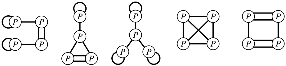
Figure 8: The Feynman diagrams for the forth order interaction term, $\langle(P\phi^{3})^{4}\rangle^{c}_{\phi}$.

By counting the number of ways to connect the legs, one can find that the degeneracies are given by $2^{3}\cdot 3^{5}$, $2^{4}\cdot 3^{5}$, $2^{3}\cdot 3^{4}$, $2^{4}\cdot 3^{4}$, and $2^{3}\cdot 3^{5}$, respectively, from the left to the right diagrams in Figure 8. These Feynman diagrams represent the ways of the index contractions of $P_{abc}^{i}$’s in the fourth order interaction term. For example, the leftmost diagram gives

$$\begin{split}&\langle(P\phi^{3})^{4}\rangle^{c,{\rm leftmost}}_{\phi}=\frac{2^{3}3^{5}}{(2\beta)^{6}}\sum_{i_{1},i_{2},i_{3},i_{4},j=1}^{R}\tilde{\Lambda}_{i_{1}j}\tilde{\Lambda}_{i_{2}j}\tilde{\Lambda}_{i_{3}j}\tilde{\Lambda}_{i_{4}j}P^{i_{1}}_{aab}P^{i_{2}}_{bcd}P^{i_{3}}_{cde}P^{i_{4}}_{eff},\end{split}$$ (83)

where the numerator of the numerical factor is the degeneracy, and the denominator comes from the factor of the Wick contraction (31). It is also straightforward to write down the explicit expressions for all the other diagrams in Figure 8.

Now let us suppose we have obtained the explicit expressions of $S^{(4)}_{eff}(P)$ by the above procedure. An immediate difficulty of this forth order term is that $S^{(4)}_{eff}(P)$ has the negative all over sign due to $I^{4}$ as in (27), and therefore the system with $S_{eff}(P)=S^{(2)}_{eff}(P)+S^{(4)}_{eff}(P)$ is not stable. This may be changed if we include the next order term $S^{(6)}_{eff}(P)$, which has a positive coefficient, but the computation will become more complicated than $S^{(4)}_{eff}(P)$ and will not be performed in this paper. To treat this situation in a consistent manner, we only take the first correction coming from $S^{(4)}_{eff}(P)$ as $e^{-S^{(4)}_{eff}(P)}\sim 1-S^{(4)}_{eff}(P)$ rather than the full exponential form. Note that this can consistently be understood as taking the first correction coming from the full expression of the interactions, $e^{-S^{(4)}_{eff}(P)-S_{eff}^{(6)}(P)-\cdots}=1-S^{(4)}_{eff}(P)-S_{eff}^{(6)}(P)+S^{(4)}_{eff}(P)^{2}/2-\cdots$, in the order of $P$. Then $f_{N,R,\Lambda_{ij}}(t)$ with this first correction of the quartic order can be obtained by computing

$$\begin{split}f^{(4)}_{N,R,\Lambda_{ij}}(t)&=const.\int dP\,e^{-S_{eff}^{(2)}(P)}(1-S_{eff}^{(4)}(P))\\ &=f^{(2)}_{N,R,\Lambda_{ij}}(t)\left(1-\langle S_{eff}^{(4)}(P)\rangle_{P}\right),\end{split}$$ (84)

where $f^{(2)}_{N,R,\Lambda_{ij}}(t)$ is given in (39), the allover constant has been determined by requiring $f^{(4)}_{N,R,\Lambda_{ij}}(0)=1$, and $\langle\cdot\rangle_{P}$ is defined by

$$\langle{\cal O}(P)\rangle_{P}:=\frac{1}{\int dPe^{-S_{eff}^{(2)}(P)}}\int dP\,{\cal O}(P)\,e^{-S_{eff}^{(2)}(P)}$$ (85)

with the quadratic action $S_{eff}^{(2)}(P)$ given in (33).

Figure 9: Graphical representations of the matrices $A$ and $\tilde{B}$.

The computation of $f^{(4)}_{N,R,\Lambda_{ij}}(t)$ in (84) has now been reduced to that of $\langle S_{eff}^{(4)}(P)\rangle_{P}$. This can be computed by the Wick theorem, using the Wick contraction for $P_{abc}^{i}$ determined from $S_{eff}^{(2)}(P)$. The Wick contraction of $P_{abc}^{i}$ can be obtained by taking the inverse of the coefficient matrix in the quadratic action $S_{eff}^{(2)}(P)$ of $P_{abc}^{i}$. Since $S_{eff}^{(2)}(P)$ has the form of the direct product with respect to the upper and lower indices, they can be treated separately.

Let us first treat the lower indices by starting with (36). Let us introduce the following matrices (See Figure 9):

$$A_{abc,def} =\frac{1}{6}\sum_{\sigma}\delta_{a\sigma_{d}}\delta_{b\sigma_{e}}\delta_{c\sigma_{f}},$$ (86)

$$B_{abc,def} =\frac{3}{N+2}\left(A\tilde{B}A\right)_{abc,def},$$ (87)

$$\tilde{B}_{abc,def} =\delta_{ad}\delta_{bc}\delta_{ef},$$ (88)

where the summation over $\sigma$ denotes the sum over all the permutations of $d,e,f$, and the product of two matrices, say $X$ and $Y$, is defined by

$$(XY)_{abc,def}=\sum_{g,h,i=1}^{N}X_{abc,ghi}Y_{ghi,def}.$$ (89)

Note that $A$ acts as the identity on a symmetric tensor, namely, $(AP)_{abc}=P_{abc}$. One can easily check the following properties:

$$A^{2}=A,\ AB=BA=B,\ B^{2}=B.$$ (90)

Furthermore, one can check that $A-B$ and $B$ give the projectors to the tensor and vector parts of $P_{abc}$, respectively, as

$$(A-B)P=P^{T},\ BP=P^{V}.$$ (91)

Therefore, by using these matrices, (38) can be rewritten in the form,

$$P\left(c_{T,\lambda_{ev}}(A-B)+c_{V,\lambda_{ev}}B\right)P,$$ (92)

where $c_{T,\lambda_{ev}}$ and $c_{V,\lambda_{ev}}$ are the coefficients associated to the tensor and vector parts of $P_{abc}$, namely,

$$\begin{split}c_{T,\lambda_{ev}}&=1+12\gamma_{3}\lambda_{ev}\,t,\\ c_{V,\lambda_{ev}}&=1+6(N+4)\gamma_{3}\lambda_{ev}\,t.\end{split}$$ (93)

The inverse of the matrix in (92) is given by

$$\begin{split}(c_{T,\lambda_{ev}}(A-B)+c_{V,\lambda_{ev}}B)^{-1}&=\frac{1}{c_{T,\lambda_{ev}}}(A-B)+\frac{1}{c_{V,\lambda_{ev}}}B\\ &=\frac{1}{c_{T,\lambda_{ev}}}A+\left(\frac{1}{c_{V,\lambda_{ev}}}-\frac{1}{c_{T,\lambda_{ev}}}\right)B.\end{split}$$ (94)

For later convenience, let us define

$$\begin{split}a_{\lambda_{ev}}&:=\frac{1}{c_{T,\lambda_{ev}}},\\ b_{\lambda_{ev}}&:=\frac{1}{c_{V,\lambda_{ev}}}-\frac{1}{c_{T,\lambda_{ev}}}.\end{split}$$ (95)

Let us next take into account the upper indices. To derive the above result we started with the expression (36) with an eigenvalue $\lambda_{ev}$ of the matrix $\Lambda_{ij}$. Therefore it is the result for the corresponding eigenspace. Considering the projection to each eigenspace, the final form of the Wick contraction for $P_{abc}^{i}$ is obtained as

$$\langle P_{abc}^{i}P_{def}^{j}\rangle_{P}=\sum_{\lambda_{ev}}\frac{1}{2}M_{\lambda_{ev}}^{ij}\left(a_{\lambda_{ev}}A+b_{\lambda_{ev}}B\right)_{abc,def},$$ (96)

where $M_{\lambda_{ev}}^{ij}$ denotes the projector to the eigenspace of the eigenvalue $\lambda_{ev}$ of $\Lambda_{ij}$.

Figure 10: An example of Wick contraction of $P_{abc}^{i}$’s. This can be computed by inserting the matrices $A$ and $B$ at the locations of contractions.

Let us next start computing $\langle S^{(4)}_{eff}(P)\rangle_{P}$ by using the Wick contraction (96). Let us first compute the factors coming from the projectors. Let us restrict ourselves to the case $\Lambda_{ij}=\lambda+\lambda_{d}\delta_{ij}$, which is of our interest as explained in Section 4. As given there, the eigenvector for $\lambda_{ev}=\lambda R+\lambda_{d}$ is $(1,1,\cdots,1)$, and those for $\lambda_{ev}=\lambda_{d}$ are the vectors transverse to that. Therefore the projectors are $M_{\lambda R+\lambda_{d}}^{ij}=1/R$ for $\lambda_{ev}=\lambda R+\lambda_{d}$, and $M_{\lambda_{d}}^{ij}=\delta_{ij}-1/R$ for $\lambda_{ev}=\lambda_{d}$, respectively. For later usage, let us compute the projectors sandwiched between $\tilde{\Lambda}_{ij}$:

$$\begin{split}&(\tilde{\Lambda}M_{\lambda_{ev}}\tilde{\Lambda})_{ij}:=\sum_{k,l=1}^{R}\tilde{\Lambda}_{ik}M_{\lambda_{ev}}^{kl}\tilde{\Lambda}_{lj}=\left\{\begin{array}[]{ll}\lambda+\frac{\lambda_{d}}{R},&\hbox{for }\lambda_{ev}=\lambda R+\lambda_{d},\\ \lambda_{d}\delta_{ij}-\frac{\lambda_{d}}{R},&\hbox{for }\lambda_{ev}=\lambda_{d},\end{array}\right.\end{split}$$ (97)

where we have used the following explicit solution to (22) for $\Lambda_{ij}=\lambda+\lambda_{d}\delta_{ij}$:

$$\tilde{\Lambda}_{ij}=p\delta_{ij}+q\hbox{ with }p^{2}=\lambda_{d},\ 2pq+Rq^{2}=\lambda.$$ (98)

As for the factor coming from the $\tilde{\Lambda}_{ij}$ in (83), the Wick contractions (96) of $P^{i}_{abc}$ will generate the factor $\sum_{j}(\tilde{\Lambda}M_{\lambda_{ev}}\tilde{\Lambda})_{jj}(\tilde{\Lambda}M_{\lambda_{ev}^{\prime}}\tilde{\Lambda})_{jj}$. Thus, using (97), we obtain the following results for each case:

$$\begin{split}&\sum_{j=1}^{R}(\tilde{\Lambda}M_{\lambda_{ev}}\tilde{\Lambda})_{jj}(\tilde{\Lambda}M_{\lambda_{ev}^{\prime}}\tilde{\Lambda})_{jj}=\left\{\begin{array}[]{cl}R\left(\lambda+\frac{\lambda_{d}}{R}\right)^{2},&\hbox{for }\lambda_{ev}=\lambda_{ev}^{\prime}=\lambda R+\lambda_{d},\\ R\left(\frac{(R-1)\lambda_{d}}{R}\right)^{2},&\hbox{for }\lambda_{ev}=\lambda_{ev}^{\prime}=\lambda_{d},\\ R\left(\lambda+\frac{\lambda_{d}}{R}\right)\frac{(R-1)\lambda_{d}}{R},&\hbox{otherwise}.\end{array}\right.\end{split}$$ (99)

It is easy to see that all the other diagrams in Figure 8 have the same factor.

As for the Wick contractions (96) of $\left(\langle(P\phi^{3})^{2}\rangle^{c}_{\phi}\right)^{2}$ in (82), there exist two cases. One is to take the contractions within each $\langle(P\phi^{3})^{2}\rangle^{c}_{\phi}$, or otherwise. The former case can be called the disconnected case, and the latter the connected case, based on their diagrammatic characters. From (32) and (96), the factors coming from the $\Lambda_{ij}$’s are obtained as

$$\sum_{i,j=1}^{R}(\Lambda M_{\lambda_{ev}})_{ii}(\Lambda M_{\lambda^{\prime}_{ev}})_{jj} =\lambda_{ev}\lambda_{ev}^{\prime}\hbox{Tr}(M_{\lambda_{ev}})\hbox{Tr}(M_{\lambda^{\prime}_{ev}})$$ (100)

$$=\left\{\begin{array}[]{cl}(\lambda R+\lambda_{d})^{2},&\hbox{for }\lambda_{ev}=\lambda_{ev}^{\prime}=\lambda R+\lambda_{d},\\ (R-1)^{2}\lambda_{d}^{2},&\hbox{for }\lambda_{ev}=\lambda_{ev}^{\prime}=\lambda_{d},\\ (\lambda R+\lambda_{d})(R-1)\lambda_{d},&\hbox{otherwise},\end{array}\right.$$ (104)

$$\sum_{i,j=1}^{R}(\Lambda M_{\lambda_{ev}})_{ij}(\Lambda M_{\lambda^{\prime}_{ev}})_{ji} =\lambda_{ev}^{2}\hbox{Tr}(M_{\lambda_{ev}})\delta_{\lambda_{ev}\lambda_{ev}^{\prime}}$$

$$=\left\{\begin{array}[]{cl}(\lambda R+\lambda_{d})^{2},&\hbox{for }\lambda_{ev}=\lambda_{ev}^{\prime}=\lambda R+\lambda_{d},\\ (R-1)\lambda_{d}^{2},&\hbox{for }\lambda_{ev}=\lambda_{ev}^{\prime}=\lambda_{d},\\ 0,&\hbox{otherwise}.\end{array}\right.$$ (108)

for the disconnected and the connected cases, respectively.

The last ingredient for the computation of $S^{(4)}_{eff}(P)$ is to take into account the lower index part of the Wick contraction (96). As can be seen in (96), in general, this is to insert $xA+yA\tilde{B}A$ with some $x,y$ at the location of the Wick contraction (See Figure 10 for an example). Diagrammatically, this is to insert the diagrams in Figure 9 at the location of the Wick contraction. This insertion generates many diagrams with a number of loops. The number of loops gives the degeneracy of each diagram in powers of $N$. The summation over all the diagrams is too many to do so by hand, so we performed this task by using Mathematica. We have obtained

$$\begin{split}G_{1}(x,y)&=6N(2+N)(4+N)(225x^{2}+90Nx^{2}+9N^{2}x^{2}+456xy\\ &+174Nxy+18N^{2}xy+232y^{2}+84Ny^{2}+8N^{2}y^{2})\end{split}$$ (109)

for $\langle(P\phi^{3})^{4}\rangle^{c}_{\phi}$. As for $\left(\langle(P\phi^{3})^{2}\rangle^{c}_{\phi}\right)^{2}$, we have obtained

$$G_{2}(x,y)= N^{2}(2+N)^{2}(4+N)^{2}(x+y)^{2},$$ (110)

$$G_{3}(x,y)= 2N(2+N)(4+N)(15x^{2}+24xy+6Nxy+8y^{2}+6Ny^{2}+N^{2}y^{2}),$$ (111)

respectively, for the disconnected and connected cases.

Let us combine all the results above. By using (96), (99) and (109) and summing over all the possibilities of the eigenspaces of $\Lambda_{ij}$, we obtain

$$\langle\langle(P\phi^{3})^{4}\rangle^{c}_{\phi}\rangle_{P}=\frac{R}{2^{2}(2\beta)^{6}}G_{1}(x_{1},y_{1}),$$ (112)

where

$$x_{1} =\left(\lambda+\frac{\lambda_{d}}{R}\right)a_{\lambda R+\lambda_{d}}+\frac{(R-1)\lambda_{d}}{R}a_{\lambda_{d}},$$ (113)

$$y_{1} =\frac{3}{N+2}\left(\left(\lambda+\frac{\lambda_{d}}{R}\right)b_{\lambda R+\lambda_{d}}+\frac{(R-1)\lambda_{d}}{R}b_{\lambda_{d}}\right).$$ (114)

For the disconnected case of $\langle\left(\langle(P\phi^{3})^{2}\rangle^{c}_{\phi}\right)^{2}\rangle_{P}$, from (96), (104) and (110) we obtain

$$\langle\left(\langle(P\phi^{3})^{2}\rangle^{c}_{\phi}\right)^{2}\rangle_{P}^{discon}=\frac{1}{2^{2}(2\beta)^{6}}G_{2}(x_{2},y_{2}),$$ (115)

where

$$x_{2} =(\lambda R+\lambda_{d})a_{\lambda R+\lambda_{d}}+(R-1)\lambda_{d}a_{\lambda_{d}},$$ (116)

$$y_{2} =\frac{3}{N+2}\left((\lambda R+\lambda_{d})b_{\lambda R+\lambda_{d}}+(R-1)\lambda_{d}b_{\lambda_{d}}\right).$$ (117)

For the connected part of $\langle\left(\langle(P\phi^{3})^{2}\rangle^{c}_{\phi}\right)^{2}\rangle_{P}$, from (96), (108) and (111) we obtain

$$\begin{split}&\langle\left(\langle(P\phi^{3})^{2}\rangle^{c}_{\phi}\right)^{2}\rangle_{P}^{con}=\frac{1}{2^{2}(2\beta)^{6}}\\ &\cdot\left((\lambda R+\lambda_{d})^{2}G_{3}(x_{3},y_{3})+(R-1)\lambda_{d}^{2}G_{3}(x_{4},y_{4})\right),\end{split}$$ (118)

where

$$\begin{split}(x_{3},y_{3})&=\left(a_{\lambda R+\lambda_{d}},\frac{3b_{\lambda R+\lambda_{d}}}{N+2}\right),\\ (x_{4},y_{4})&=\left(a_{\lambda_{d}},\frac{3b_{\lambda_{d}}}{N+2}\right).\end{split}$$ (119)

By putting (112), (115) and (118) into (82), we obtain the final result given in (41) and (42).

Appendix Appendix E Estimation of the $R$-dependence of $b_{1}$

As for $b_{1}$, there are two kinds of contributions as given in (82). The dominant $R$-dependence of the former term of (82) can be estimated by considering the expression (83), because the contractions of the upper indices among $P^{i}_{abc}$ are the same for all the diagrams in Figure 8. It is sufficient to consider $\lambda_{d}=0$, since this is of our interest, and the mode of $P^{i}_{abc}$ contributing in this case with the appropriate normalization has the form $\frac{1}{\sqrt{R}}(1,1,\ldots,1)P_{abc}$, which has the form of the eigenvector of the matrix $\Lambda_{ij}=\lambda$ for the eigenvalue $\lambda R$. Since $\tilde{\Lambda}_{ij}\sim 1/\sqrt{R}$ (see (98)) and there are five free summations over the upper indices in (83), the former term of (82) is estimated as

$$b_{1}^{former}\sim\gamma_{6}R^{5}\sqrt{R}^{-4}\sqrt{R}^{-4}\sim R^{-5}.$$ (120)

As for the latter term of (82), $\langle(P\phi^{3})^{2}\rangle^{c}_{\phi}\sim RP^{2}$ by a similar argument as above. Therefore,

$$b_{1}^{latter}\sim(\gamma_{3}^{2}-\gamma_{6})R^{2}\sim R^{-5},$$ (121)

where it is important to note that the contents of the parentheses give $R^{-7}$ due to the cancellation of the leading $R^{-6}$ terms of both.

The above two estimations conclude $b_{1}\sim R^{-5}$.

Appendix Appendix F Brief introduction of persistent homology

In this appendix, we give a brief introduction of persistent homology for this paper to be self-contained. More details can be found for instance in [30].

Persistent homology is a notion that characterizes the topological aspects of a data in terms of homology. A data to be analyzed should be a set of points with relative distances. From a data, a stream (or a filtration) of simplicial complexes parameterized by a scale parameter, say $u$, is constructed. The details of the construction of a stream will be given at the end of this appendix. Once a stream is constructed, the homology groups of the simplicial complexes at each value of $u$ are computed. By increasing the value of $u$ from zero, a homology group element will appear at a certain value of $u$, say $u_{\rm start}$, and will continue to exist until it disappears at another value, say $u_{\rm end}$. If the life period $u_{\rm end}-u_{\rm start}$ is large, one may regard the element as a persistent homology group element, which has a long life. The collection of persistent homology group elements characterizes the topological property of a data set. There will also be a number of short-life elements, but they are often regarded as “noises”, which are not robust against small perturbations of the data. Roughly speaking, the scale $u$ parameterizes the sizes of topological structure of interest, and persistent homology characterizes a data with multi-scale homology groups.

There are two kinds of diagrams that are convenient for visualizing the persistent homology of a data. One is called barcode diagram, where each horizontal line segment $[u_{start},u_{end}]$ represents a homology group element that exists during the period. An example of barcode diagrams constructed from a sample of $\phi_{a}^{i}$ generated in the Monte Carlo simulation is shown in Figure 11. How to construct a set of points with relative distances from $\phi_{a}^{i}$ is given in Section 7. The left figure shows the barcode diagram for the 0-dimensional homology, and the right that for the 1-dimensional homology. The left diagram indicates that the initially separated points form one connected component over the scale $u\sim 1.4$. The right figure shows that there exists a one-dimensional cycle which has the size of $u\sim 1.8$, while there is a small “noise” around $u\sim 0.9$. In Figure 12, we provide the graph constructed by connecting the points with relative distances $u<1.5$, using the same $\phi_{a}^{i}$ for Figure 11. One can actually see the presence of a one-dimensional cycle consistent with the barcode diagram.

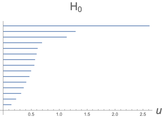
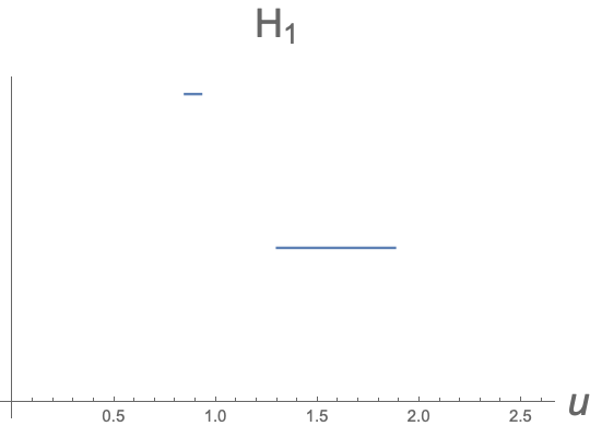
Figure 11: An example of barcode diagrams. The example is obtained by analyzing a configuration $\phi_{a}^{i}\ (i=1,2,\ldots,R)$ generated by the actual Monte Carlo simulation for $N=4$, $R=15$, and $k=0.01$. The presence of a long-life one-dimensional homology group element can be observed in this particular data.

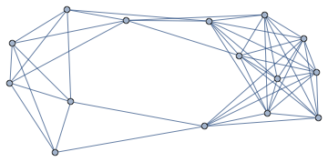
Figure 12: A graph made by connecting the points with relative distances smaller than $1.5$. The data is the same one used for Figure 11. This choice of the distance cut-off is made because a one-dimensional cycle is expected to exist at this scale, seeing the right of Figure 11.

The other kind of diagram is called persistent diagram. An element that is represented by a line segment $[u_{\rm start},u_{\rm end}]$ in a barcode diagram is represented by a dot located at the two-dimensional coordinate $(u_{\rm start},u_{\rm end})$ in a persistent diagram. Since there are multiple elements in general, and $u_{\rm start}<u_{\rm end}$, a persistent diagram consists of a number of dots in the region over the diagonal line. The long-life elements are represented by the dots that exist away from the diagonal line, and those in the vicinity of the diagonal line are regarded as “noises”. An example of a persistent diagram is given in Figure 13, which corresponds to the right barcode diagram in Figure 11. What is convenient in a persistent diagram is that one can easily superimpose persistent diagrams from multiple data. If there is a common characteristics through multiple data, one can find it as a characteristic pattern in a superimposed persistent diagram. Therefore, we use persistent diagrams to find statistically favored structure common in the configurations generated by the Monte Carlo simulation.

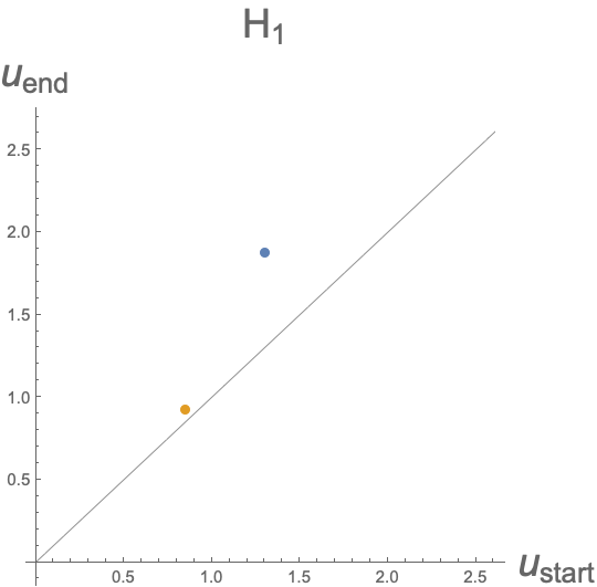
Figure 13: The persistent diagram corresponding to the right barcode diagram in Figure 11. A line segment in a barcode diagram is represented by a dot in a persistent diagram. The longest one is represented by a blue dot, and the second by a yellow one. The colors are also used in the persistent diagrams in Section 7.

Let us finally explain the actual construction of a stream of simplicial complexes parameterized by $u$. In fact, there exist various streams depending on purposes in the literature, but let us restrict ourselves to the Vietoris-Rips stream, which is used in the open-source c++ code called Ripser. For a given data that stores distances between points, the Vietoris-Rips stream ${\rm VR}(V,u)$ is defined as follows:

• The vertex set is given by the point set $V$ of a data.

• For vertices $i$ and $j$ with distance $d(i,j)$, the edge $[i,j]$ are included in ${\rm VR}(V,u)$, if and only if $d(i,j)\leq u$.

• A higher-dimensional simplex is included in ${\rm VR}(V,u)$, if and only if all of its edges are.

From the above definition, there is an obvious property, ${\rm VR}(V,u)\subset{\rm VR}(V,u^{\prime})$ for $u<u^{\prime}$. An important fact is that this induces a map: ${\rm H}_{k}({\rm VR}(V,u))\rightarrow{\rm H}_{k}({\rm VR}(V,u^{\prime}))$ for $u<u^{\prime}$. Therefore, the development of each homology group element under the change of the value of $u$ can be followed, and its life is characterized by the two endpoint values of $u$. This makes barcode and persistent diagrams convenient ways for the description.

References

- [1] M. Reuter and F. Saueressig, “Quantum Gravity and the Functional Renormalization Group : The Road towards Asymptotic Safety,” Cambridge University Press, 2019.
- [2] R. Loll, “Quantum Gravity from Causal Dynamical Triangulations: A Review,” arXiv:1905.08669 [hep-th].
- [3] C. Rovelli and F. Vidotto, “Covariant Loop Quantum Gravity : An Elementary Introduction to Quantum Gravity and Spinfoam Theory,” Cambridge University Press, 2014.
- [4] S. Surya, “The causal set approach to quantum gravity,” arXiv:1903.11544 [gr-qc].
- [5] T. Konopka, F. Markopoulou and L. Smolin, “Quantum Graphity,” hep-th/0611197.
- [6] E. Wigner, “Characteristic vectors of bordered matrices with infinite dimensions”, Annals of Mathematics 62 (3): 548-564.
- [7] G. ’t Hooft, “A planar diagram theory for strong interactions,” Nucl. Phys. B 72, 461 (1974).
- [8] E. Brezin and V. A. Kazakov, “Exactly Solvable Field Theories of Closed Strings,” Phys. Lett. B 236, 144 (1990). doi:10.1016/0370-2693(90)90818-Q
- [9] M. R. Douglas and S. H. Shenker, “Strings in Less Than One-Dimension,” Nucl. Phys. B 335, 635 (1990). doi:10.1016/0550-3213(90)90522-F
- [10] D. J. Gross and A. A. Migdal, “Nonperturbative Two-Dimensional Quantum Gravity,” Phys. Rev. Lett. 64, 127 (1990). doi:10.1103/PhysRevLett.64.127
- [11] J. Ambjorn, B. Durhuus, and T. Jonsson, “Three-dimensional simplicial quantum gravity and generalized matrix models,” Mod. Phys. Lett. A06 (1991) 1133–1146.
- [12] N. Sasakura, “Tensor model for gravity and orientability of manifold,” Mod. Phys. Lett. A06 (1991) 2613–2624.
- [13] N. Godfrey and M. Gross, “Simplicial quantum gravity in more than two-dimensions,” Phys. Rev. D43 (1991) R1749–1753.
- [14] R. Gurau, “Colored Group Field Theory,” Commun. Math. Phys. 304, 69 (2011) doi:10.1007/s00220-011-1226-9 [arXiv:0907.2582 [hep-th]].
- [15] G. Narain, N. Sasakura and Y. Sato, “Physical states in the canonical tensor model from the perspective of random tensor networks,” JHEP 1501, 010 (2015) doi:10.1007/JHEP01(2015)010 [arXiv:1410.2683 [hep-th]].
- [16] N. Sasakura, “Canonical tensor models with local time,” Int. J. Mod. Phys. A 27, 1250020 (2012) doi:10.1142/S0217751X12500200 [arXiv:1111.2790 [hep-th]].
- [17] N. Sasakura, “Uniqueness of canonical tensor model with local time,” Int. J. Mod. Phys. A 27, 1250096 (2012) doi:10.1142/S0217751X12500960 [arXiv:1203.0421 [hep-th]].
- [18] D. Obster and N. Sasakura, “Emergent symmetries in the canonical tensor model,” PTEP 2018, no. 4, 043A01 (2018) doi:10.1093/ptep/pty038 [arXiv:1710.07449 [hep-th]].
- [19] T. Kawano, D. Obster and N. Sasakura, “Canonical tensor model through data analysis: Dimensions, topologies, and geometries,” Phys. Rev. D 97, no. 12, 124061 (2018) doi:10.1103/PhysRevD.97.124061 [arXiv:1805.04800 [hep-th]].
- [20] D. Obster and N. Sasakura, “Symmetric configurations highlighted by collective quantum coherence,” Eur. Phys. J. C 77, no. 11, 783 (2017) doi:10.1140/epjc/s10052-017-5355-y [arXiv:1704.02113 [hep-th]].
- [21] L. Lionni and N. Sasakura, “A random matrix model with non-pairwise contracted indices,” PTEP 2019, no. 7, 073A01 (2019) doi:10.1093/ptep/ptz057 [arXiv:1903.05944 [hep-th]].
- [22] A. Anderson, R. C. Myers and V. Periwal, “Complex random surfaces,” Phys. Lett. B 254, 89 (1991).
- [23] A. Anderson, R. C. Myers and V. Periwal, “Branched polymers from a double scaling limit of matrix models,” Nucl. Phys. B 360, 463 (1991).
- [24] R. C. Myers and V. Periwal, “From polymers to quantum gravity: Triple scaling in rectangular random matrix models,” Nucl. Phys. B 390, 716 (1993) [hep-th/9112037].
- [25] S. Nishigaki and T. Yoneya, “A nonperturbative theory of randomly branching chains,” Nucl. Phys. B 348, 787 (1991). doi:10.1016/0550-3213(91)90215-J
- [26] P. Di Vecchia, M. Kato and N. Ohta, “Double scaling limit in O(N) vector models in D-dimensions,” Int. J. Mod. Phys. A 7, 1391 (1992). doi:10.1142/S0217751X92000612
- [27] A. Crisanti and H.-J. Sommers, “The spherical p-spin interaction spin glass model: the statics,” Z. Phys. B 87, 341 (1992).
- [28] T. Castellani and A. Cavagna, “Spin-glass theory for pedestrians”, J. Stat. Mech.: Theo. Exp. 2005, 05012 [arXiv: cond-mat/0505032].
- [29] N. Sasakura, “Quantum canonical tensor model and an exact wave function,” Int. J. Mod. Phys. A 28, 1350111 (2013) doi:10.1142/S0217751X1350111X [arXiv:1305.6389 [hep-th]].
- [30] G. Carlsson, “Topology and data,” Bulletin of the American Mathematical Society, 46(2), 255-308, DOI: 10.1090/S0273-0979-09-01249-X.
- [31] P. Di Francesco, P. H. Ginsparg and J. Zinn-Justin, “2-D Gravity and random matrices,” Phys. Rept. 254, 1 (1995) [hep-th/9306153].
- [32] J. Nestruev, Smooth Manifolds and Observables, Springer, 2003.
- [33] N. Sasakura, “Tensor model and dynamical generation of commutative nonassociative fuzzy spaces,” Class. Quant. Grav. 23, 5397 (2006) doi:10.1088/0264-9381/23/17/017 [hep-th/0606066].
- [34] N. Sasakura, “The Fluctuation spectra around a Gaussian classical solution of a tensor model and the general relativity,” Int. J. Mod. Phys. A 23, 693 (2008) doi:10.1142/S0217751X08038536 [arXiv:0706.1618 [hep-th]].
- [35] N. Sasakura, “The Lowest modes around Gaussian solutions of tensor models and the general relativity,” Int. J. Mod. Phys. A 23, 3863 (2008) doi:10.1142/S0217751X0804130X [arXiv:0710.0696 [hep-th]].
- [36] N. Sasakura, “Emergent general relativity on fuzzy spaces from tensor models,” Prog. Theor. Phys. 119, 1029 (2008) doi:10.1143/PTP.119.1029 [arXiv:0803.1717 [gr-qc]].
- [37] N. Sasakura, “Gauge fixing in the tensor model and emergence of local gauge symmetries,” Prog. Theor. Phys. 122, 309 (2009) doi:10.1143/PTP.122.309 [arXiv:0904.0046 [hep-th]].
- [38] N. Sasakura and Y. Sato, “Constraint algebra of general relativity from a formal continuum limit of canonical tensor model,” JHEP 1510 (2015) 109 doi:10.1007/JHEP10(2015)109 [arXiv:1506.04872 [hep-th]].
- [39] H. Chen, N. Sasakura and Y. Sato, “Equation of motion of canonical tensor model and Hamilton-Jacobi equation of general relativity,” Phys. Rev. D 95, no. 6, 066008 (2017) doi:10.1103/PhysRevD.95.066008 [arXiv:1609.01946 [hep-th]].
- [40] N. Sasakura and Y. Sato, “Interpreting canonical tensor model in minisuperspace,” Phys. Lett. B 732, 32 (2014) doi:10.1016/j.physletb.2014.03.006 [arXiv:1401.2062 [hep-th]].