The integration of variable generation and storage into electricity capacity markets

Abstract

We show how to value both variable generation and energy storage to enable them to be integrated fairly and optimally into electricity capacity markets. We develop theory based on balancing expected energy unserved against costs of capacity procurement, and in which the optimal procurement is that necessary to meet an appropriate reliability standard. For conventional generation the theory reduces to that already in common use. Further the valuation of both variable generation and storage coincides with the traditional risk-based approach based on equivalent firm capacity. The determination of the equivalent firm capacity of storage requires particular care; this is due both to the flexibility with which storage added to an existing system may be scheduled, and also because, when any resource is added to an existing system, storage already within that system may be flexibly rescheduled. We illustrate the theory with an example based on the GB system.

Keywords: Capacity markets, variable generation, storage.

1 Introduction

In order to ensure the adequacy of electricity supplies many systems, including those of Great Britain and other European countries and several North American regions, now provide a capacity market—see, e.g., [10, 21, 16, 12, 18, 13]. (Others, e.g. those of Australia and Texas, continue to rely on energy-only markets.) So as to operate such a market both fairly and optimally it is necessary to value appropriately (i.e. mathematically correctly) the contributions of the individual capacity providers, whether they provide conventional generation, variable generation, or storage. Present approaches to capacity market design have primarily been designed with conventional generation in mind, e.g. in GB ([18]) and in North America ([3, 16]). Conventional generation is typically approximated as firm capacity, where we define the latter as idealised capacity which is always available to supply energy as needed up to a given constant rate. (To do so nominal generator capacities are usually multiplied by appropriate “de-rating” factors to acknowledge occasional unavailability—see [18, 3].)

When all capacity is capable of being approximated as if it were firm, an economic theory of capacity markets is straightforward, and may be based on balancing procurement cost against cost of unserved energy ([24, 27]). [2] consider the impact on societal welfare of the (mathematically) incorrect de-rating of variable generation, but consider neither storage nor the mechanism of running a capacity market. The need to rapidly reduce fossil fuel dependence means that both variable generation—e.g. wind and solar power—and storage now have increasingly important contributions to make to capacity adequacy ([9]). The present paper shows how current approaches to capacity market design may be extended to give an integrated theory for the inclusion within a capacity market of all types of capacity provision. As at present, the theory is necessarily based on a probabilistic description of the electricity supply-demand balance process. However, storage has a natural energy constraint and thus can supply energy only for a limited period of time before needing to be replenished; subject to this constraint it may be scheduled flexibly. Hence, in order to understand both how to schedule storage and to determine its contribution to capacity adequacy, it is necessary to pay attention to the sequential statistical structure of the supply-demand balance process to which that storage is contributing—see Sections 2 and 3. The present paper extends and generalises theory which was developed by the authors in conjunction with National Grid ESO for the integration of storage into the GB capacity market ([19]). However, the theory is applicable wherever capacity contributions of variable generation and storage need to be correctly assessed. This includes the European and North American markets referenced above.

The determination of a volume of capacity-to-be-procured in a capacity market may be achieved either via the satisfaction of an appropriate security-of-supply standard defined in terms of some given system risk metric, or via the minimisation of an appropriate economic cost. (In the latter case the capacity-to-procure may be variable and specified as a function of the clearing price in the capacity auction; this is what currently happens in GB.) These two approaches are closely related—see Section 5. In either case, a key step in the development of an integrated theory is that of the provision of an appropriate definition of the equivalent firm capacity (EFC) of any capacity-providing resource. This EFC is the firm capacity which makes an (appropriately defined) equivalent contribution to the overall supply-demand balance. Hence the EFC is necessarily defined with respect to the pre-existing supply-demand balance process to which this resource is being added ([26, 5]). When the set of capacity-providing resources contains significant storage, particular care is required in the determination of EFCs. One reason for this is the need to account for the flexibility of scheduling of additional storage added to an existing supply-demand balance process. More subtly, when any further resource—including, for example, firm capacity—is added to an existing set of capacity-providing resources which already contains storage, that pre-existing storage may also be rescheduled so as to enhance the usefulness of the additional contribution. A consequence, as we show formally at the end of Section 3 and demonstrate in the example of Section 6, is that the EFC of further storage added to an existing system is less (than it would otherwise be) in the case where that additional system already contains significant storage.

Throughout the present paper we treat the process of electricity demand as given. However, demand response may also be used to assist in balancing systems. Demand response has many of the characteristics of storage, typically making a similarly flexible contribution. Its contribution to electricity capacity, and its integration into capacity markets, may be analysed analogously. However, in present day markets it is often treated as demand which may be effectively foregone—see [15] for a review, and also [19].

Sections 2 and 3 of the paper study respectively risk metrics and EFC. The latter is necessarily defined in terms of some risk metric and is essential to the understanding of both capacity adequacy and the operation of a capacity market. The studied properties are implicit in the theory of present markets for what is mostly conventional generation. However, so as to understand how to incorporate into such markets both variable generation and time-limited but flexible resources such as storage, it is necessary to make these properties explicit. It is further necessary to make explicit assumptions of continuity and smoothness as available capacity-providing resource is varied. We argue that these assumptions, which are often implicit in other work (e.g. [2]), are usually sufficiently satisfied in practice. The smoothness assumption yields an important local additivity property for EFCs; this is essential for the optimal operation of markets—even in the case where all resource is provided by firm capacity. In Section 3 we also show how to determine the EFCs of marginal contributions of both variable generation and storage, notably when the objective is the minimisation of expected energy unserved (EEU). For storage this requires consideration of how it may be optimally scheduled.

Section 4 studies the operation of capacity markets when the objective is that of obtaining at minimum cost sufficient capacity to meet a given security-of-supply standard defined in terms of a risk metric. Section 5 studies the operation of such markets when the objective is that of the minimisation of an overall economic cost. The present economic theory of such markets requires substantial modification in the presence of variable generation and, especially, storage.

The flexibility of storage scheduling has important consequences for the way in which a capacity market operates, and these are illustrated in the detailed example of Section 6. This example shows the application of nearly all the above theory, and is chosen to be realistic in the context of a country such as GB. It further demonstrates the practical reasonableness of the assumptions required for a tractable theory.

2 Risk metrics

In the analysis of capacity adequacy, the length of time over which system risk is assessed—typically a year or a peak season—is usually divided into $n$ time periods, each typically of an hour or a half-hour in length ([1, 19]). Let random variables $D_{t}$ and $X_{t}$ denote respectively the total energy demand and total energy supply in time period $t$. Then the supply-demand balance in the time period $t$ is given by the random variable $Z_{t}=X_{t}-D_{t}$. Values of $Z_{t}$ less than zero correspond to an energy shortfall or loss-of-load at time $t$. The depth of shortfall at that time is given by the random variable $\max(-Z_{t},0)$.

Any risk metric $\rho$ is a function of the entire process $(Z_{t},\,t=1,\dots,n)$. Risk metrics may either be used directly in the setting of reliability standards—as in the case of the present GB $\mathrm{LOLE}$-based standard ([19])—or may arise naturally in economic approaches to determining security-of-supply (see Section 5).

LOLE and EEU.

The two most commonly used risk metrics are loss-of-load expectation (LOLE) and expected energy unserved (EEU), given respectively by

$$\mathrm{LOLE} =\sum_{t=1}^{n}\mathbf{P}(Z_{t}<0),$$ (1)

$$\mathrm{EEU} =\sum_{t=1}^{n}\mathbf{E}(\max(-Z_{t},0))=\sum_{t=1}^{n}\int_{-\infty}^{0}\mathbf{P}(Z_{t}<z)\,dz,$$ (2)

where $\mathbf{P}$ denotes probability and $\mathbf{E}$ denotes expectation ([1, 14, 26]). It follows from the additivity of expectations that, in discrete time, LOLE is the expected number of periods of shortfall during the season under study, while EEU is the expectation of the sum of the depths of shortfall during such periods, i.e. the expectation of the total unserved energy.

The use of EEU as a measure of economic cost corresponds to a uniform valuation of unserved energy, regardless of the overall depth of energy shortfall at any given time and also of the overall duration of the energy shortfall periods. The present paper mainly considers such a uniform valuation. However, often modest depths or durations of shortfall may be managed without significant ill effects, while the avoidance of economic damage becomes increasingly difficult as depth or duration of shortfall increases. Thus it may sometimes be natural to value unserved energy more highly at higher levels of shortfall.

However, security-of-supply standards are presently more commonly defined via the use of the LOLE risk metric. This metric might be regarded as naturally somewhat flawed, in that—unlike EEU, which values periods of energy shortfall in proportion to their depth—LOLE takes no account of shortfall depth. Furthermore, we argue below that, in the presence of either variable generation or storage, LOLE is a poor measure of system reliability. This is especially so in the case of storage. We give the relevant mathematics in Section 5, but the following simple example illustrates why the use of LOLE may be problematic. Suppose that a certain volume of stored energy is available to mitigate, but not wholly eliminate, a given period of energy shortfall. The loss-of-load duration, and hence LOLE, is minimised by using this additional stored energy to eliminate entirely the shortfall at those times within the above period at which this is most efficiently achieved, i.e. at those times at which the depth of the original shortfall is least. The reason is that this policy maximises the total length of time for which there is no longer any loss-of-load—see the left panel of Figure 1, which shows an illustrative pattern of shortfall as above, and the reduction (shaded) in that shortfall when the stored energy is used to minimise loss-of-load. However, it might reasonably be argued that in practice the available stored energy would be at least as well employed in instead minimising the maximum depth of shortfall in supply during the period concerned. The latter policy which would achieve the same reduction in unserved energy but quite possibly result in no reduction in loss-of-load whatsoever—see the middle panel of Figure 1 which shows the reduction in shortfall (again shaded) when the same stored energy is now used in this way. Indeed, from an economic perspective, the latter policy would clearly be better if the unit cost of unserved energy were an increasing function of shortfall depth. Further, regardless of how unserved energy is valued, the former policy of using stored energy to minimise loss-of-load does not make as effective a contribution to system reliability as would the use of firm capacity to achieve the same reduction in loss-of-load: unlike storage such firm capacity would continue to contribute even at those times when shortfall was not completely eliminated—see the right panel of Figure 1 which shows (again for the same pattern of initial shortfall) the shaded reduction in shortfall which occurs when firm capacity is used to achieve the same loss-of-load duration as in the left panel.

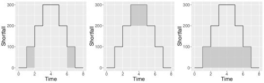
Figure 1: Use of a given volume of storage to mitigate a given period of shortfall, and comparison with firm capacity.

The above difficulties in measuring the contribution of storage arise on account of its time-limited duration combined with its flexibility of use. In the presence of storage, LOLE may be varied in a manner which (as illustrated above) does not obviously relate to system adequacy as usually understood. To a lesser extent there may be analogous difficulties with variable generation ([2]); however, unlike storage, the times at which variable generation is available are not controllable. When capacity is provided solely via conventional generation, and when the latter is capable of being modelled as if it were (de-rated) firm capacity, then within a given system the relation of LOLE to an economic measure of system adequacy such as EEU is essentially predetermined, and the above difficulties do not then arise. We give a more precise mathematical treatment in Sections 4 and 5.

General risk metrics.

We take as given the demand process $(D_{t},\,t=1,\dots,n)$. The energy supply process $(X_{t},\,t=1,\dots,n)$, and hence the value of any risk metric, is determined by the set of capacity-providing resources (conventional generation, variable generation, and storage). We denote by $R$ the set of such resources, and regard any risk metric $\rho$ as a function $\rho{(R)}$ of the set $R$. For a coherent theory, we assume that the resources within $R$ are optimally used for the minimisation of overall system risk. This assumption is needed in the context of flexible resources such as storage which may be used in different ways to support the system—however, see Section 3. We assume, as is usual, that any risk metric $\rho$ is such that $\rho(R)$ is decreasing as the set of resources $R$ is increased.

Typically, for a large system, the effect on its overall state—as measured by the risk metric—of the addition or subtraction of a single unit of resource is small. The optimality of the state of the system (by some criterion) is typically characterised by some form of equilibrium with respect to marginal, i.e. relatively small, variations in that overall state caused by the addition or subtraction of individual resources. So as to obtain a reasonable and tractable economic theory, we require continuity and smoothness assumptions with respect to such marginal variations. The continuity assumption is that of reasonably continuous availability of capacity, i.e. that the state of the macroscopic system may be varied continuously—at least to a good approximation—by the addition or subtraction of individual units of capacity-providing resource. In large systems this is a reasonable approximation which is usually made in the design of current capacity markets. An exception occurs when considering some very large individual resource, e.g. a large nuclear plant; however, it is straightforward to deal with a small number of such large contributions—see Section 4. The smoothness assumption is that, for any set of resources $R$, the reduction in risk $\rho(R)-\rho(R+i)$ resulting from the addition of some further marginal resource $i$ to the set $R$ (where, for simplicity, we denote the resulting set of resources by $R+i$) is, to a good approximation, unchanged by small variations in the set $R$. More formally, this is the requirement that, for any small resource $j$ (representing the above variation in the set $R$) and for any further small resource $i$, to a good approximation

$$\rho(R+i+j)-\rho(R+j)=\rho(R+i)-\rho(R),$$ (3)

where, as above, $R+i+j$ denotes the set of resources $R$ supplemented by the further resources $i$ and $j$, and where, as the contribution of the resource $j$ reduces in size, the percentage error in the relation (3) becomes negligible. This smoothness assumption is essentially a form of differentiability assumption—see below—and is generally well satisfied in most applications and for most risk metrics. In the extended example of Section 6, which is chosen to be reasonably representative of a system such as that in GB, we check the applicability of both the above assumptions.

The concept of firm capacity, defined as energy supply which is guaranteed to be available up to a given constant rate throughout the overall period under consideration, plays a role as a reference measure in assessing the usefulness of other forms of resource—see Section 3. In considering variations about the set of resources $R$ given by variations in firm capacity, we also write (analogously to the above) $R+y$ for the set of resources $R$ supplemented by firm capacity able to supply energy at a further constant rate $y$; we further allow that $y$ may be continuously varied. This will be important when we consider equivalent firm capacity below. It is straightforward to show that, for such variation, the above smoothness assumption implies that there exists the derivative $\rho^{\prime}(R)$ of $\rho(R)$ with respect to firm capacity; this is such that, for small variations of the total resource $R$ by firm capacity $y$,

$$\rho(R+y)=\rho(R)+\rho^{\prime}(R)y,$$ (4)

(the relative error in this approximation tending to zero as $y$ tends to zero). This derivative plays an important role in subsequent analysis.

3 Equivalent Firm Capacity

We take as given a suitable risk metric $\rho$. Then, given also any set of capacity-providing resources $R$, the contribution of any further resource $i$ (conventional generation, variable generation, or storage) to be added to the set $R$ may be measured by its equivalent firm capacity (EFC) $\mathit{efc}_{R}(i)$. This is the firm capacity which, if added to the set $R$ in place of the additional resource $i$, would make the same contribution to security-of-supply, as measured by the risk metric $\rho$. Formally, the constant $\mathit{efc}_{R}(i)$ is the solution of

$$\rho(R+i)=\rho(R+\mathit{efc}_{R}(i)),$$ (5)

where, as defined earlier, the notations $R+i$ and $R+\mathit{efc}_{R}(i)$ correspond to the set of resources $R$ supplemented respectively by the resource $i$ and by firm capacity $\mathit{efc}_{R}(i)$ (see, e.g., [14, 26, 19]). When the set $R$ contains resources such as storage which may be flexibly used, the addition of further resource may result in a different pattern of usage of the resources within $R$ itself: on both the left and the right side of (5) it is assumed that the total available resource is being optimally used—see also below for a discussion of the practicality of this. When the resource $i$ is itself firm capacity $y_{i}$ for some $y_{i}>0$, then $\mathit{efc}_{R}(i)=y_{i}$ independently of $R$. However, in general the EFC of a resource, e.g., variable generation or storage, depends also on the existing set of resources $R$ to which it is being added ([26, 5]). This will be important in Sections 4 and 5 for developing satisfactory theories of capacity adequacy and capacity markets.

It follows from (4) and (5) that, for the addition of any marginal (i.e. small) resource $i$ to the set $R$,

$$\rho(R+i)=\rho(R)+\rho^{\prime}(R)\mathit{efc}_{R}(i),$$ (6)

(where the derivative $\rho^{\prime}(R)$ in (6) remains, as in (4), that defined with respect to variation in firm capacity). Thus, for any existing set of resources $R$, and with respect to the risk metric $\rho$, the contribution to risk reduction given by any further marginal resource $i$ is proportional to its EFC $\mathit{efc}_{R}(i)$. It hence makes sense to value such additional resources proportionally to their EFCs—see Section 4. The smoothness assumption (3) further implies the local additivity of the EFCs of marginal (i.e. small) variations about the set $R$, i.e., for marginal additions $i$ and $j$ to $R$,

$$\mathit{efc}_{R}(i,j)=\mathit{efc}_{R}(i)+\mathit{efc}_{R}(j),$$ (7)

where by the left side of (7) is meant the EFC of the combined resources $i$ and $j$, and where the relative error in (7) again becomes negligible as the additional resources $i$ and $j$ reduce in size. The property (7) is a straightforward consequence of (3) and (6): the substitution of each term in (3) by the expression given by (6) yields (7) immediately. The local additivity result (7) is, like the smoothness assumption itself, a form of differentiability. It is a weaker property than full additivity, i.e. it does not hold in the case of larger variations about the set $R$. This is something which is well-known and which we discuss further in Section 4 and illustrate in Section 6.

Determination of EFCs.

The EFC $\mathit{efc}_{R}(i)$ of any capacity-providing resource $i$ added to an existing set of resources $R$ is defined by the solution of equation (5). The solution of (5) may involve trial values of $\mathit{efc}_{R}(i)$ and may not always be straightforward. Provided that the additional resource $i$ is marginal (i.e. small) in relation to the existing set $R$, then it is generally more straightforward to obtain the EFC $\mathit{efc}_{R}(i)$ of the further resource $i$ via the solution of (6) above, i.e. as

$$\mathit{efc}_{R}(i)=\frac{\rho(R+i)-\rho(R)}{\rho^{\prime}(R)};$$ (8)

typically all the quantities on the right side of (8) may be readily estimated, e.g. via simulation. (Recall that (8) is ultimately a consequence of the earlier smoothness assumption, the validity of which we check in our extended example of Section 6.)

As we argue in Sections 2 and 5, it is often natural to take the underlying risk metric $\rho$ to be given by EEU. Then, in order to use (8), we require an expression for the derivative $\mathrm{EEU}^{\prime}(R)$ of $\mathrm{EEU}(R)$ with respect to firm capacity. For any set of capacity-providing resources $R$ which consists entirely of generation, conventional or variable, we have

$$\mathrm{EEU}^{\prime}(R)=-\mathrm{LOLE}(R).$$ (9)

The result (9) is known in the case where all the resource within the set $R$ is provided by firm capacity (see [6]); its proof in the present case—where $R$ may also contain variable generation (but not storage)—is essentially the same and is given in the appendix. The results (8) and (9) therefore provide an efficient way to determine the EFCs (with respect to the risk metric given by EEU) of marginal contributions to capacity in an environment in which all capacity is provided by generation—a result which is also implicit in [2]. The result (9) is also important in an economic theory of capacity markets—see Section 5.

When the set of resources $R$ includes storage, the result (9) requires modification. The reason for this is that when further resource—including firm capacity—is added to an existing set of resources, the use of any storage within that set may be rescheduled so as to continue to contribute optimally to the minimisation of EEU, thereby increasing the contribution of the additional resource. Thus the right side of (9) needs to be replaced by something which is larger in absolute value.

For an exact analysis, assume that storage may be completely recharged between periods of what would, in the absence of storage, be energy shortfall, but that storage may not usefully be recharged during periods of shortfall. (This is currently the case in GB, for example, where periods of shortfall are generally well separated; typically there is at most a single period of shortfall during any day, and storage may be fully recharged overnight.) Assume also that any process of what would otherwise be continuous energy shortfall is met as far as possible from available storage, with the aim of minimising residual unserved energy, and that each store $i$ delivers energy subject to rate (power) and total energy constraints. At each time $t$ define the residual lifetime of each store $i$ as such residual energy in the store at time $t$ as is available for subsequent use divided by the maximum rate at which that energy can be served. Then the above minimisation of EEU is achieved by the use of the greedy algorithm in which, at each successive time $t$ during any period of shortfall, this shortfall is reduced as far as possible from energy in storage and in which the use of the stores is prioritised in descending order of their residual lifetimes. The optimality of the above policy is proved by [4] and by [8]. Note that the implementation of this policy, although optimal, nevertheless does not, as each successive time $t$, require any foreknowledge of the shortfall process subsequent to time $t$, so that this policy is practicable to the extent that the scheduling of stores may be coordinated. (If, in more extreme situations, storage may not be fully recharged between periods of use, then optimal scheduling is more complicated and does require foresight as above. This is also the case when the unit valuation of unserved energy is not uniform but increases according to the depth of shortfall, in which case it is sometimes optimal to defer serving energy from storage in anticipation of its being more usefully supplied at a later time—see [4] for a detailed analysis.) Even when such coordination is difficult, under the above assumption that storage may not be recharged within shortfall periods, any policy for the use of the stores which does not actually spill energy will clearly also perform optimally in any shortfall period in which either the stores are emptied or the shortfall eliminated, so that most reasonable policies for the use of storage may generally be expected to work well—again see [4]. Let $S_{e}$ be the set of stores which, under the above optimal policy, are empty (i.e. have reached their minimum permitted state of charge) at the end of the shortfall period. Then it is formally shown by [4] that, in the presence of storage, the result (9) is replaced by the more general result

$$\mathrm{EEU}^{\prime}(R)=-\mathrm{LOLE}(R\setminus S_{e}),$$ (10)

where $R\setminus S_{e}$ is the set of resources in $R$ other than those in the set $S_{e}$. (Since the shortfall process is typically random, so also is the set $S_{e}$. Thus if, for example, the right side of (10) were being evaluated by simulation, for each such simulation the set $S_{e}$ and the loss-of-load corresponding to $R\setminus S_{e}$ would both be observed; the latter would then be averaged over simulations to estimate $\mathrm{LOLE}(R\setminus S_{e})$.)

As observed above, when firm capacity is added to a set of resources $R$, it contributes more effectively to the reduction of EEU when the set $R$ already contains storage resources which may then be rescheduled. As a simple example, consider a shortfall of 100 MW for one hour followed by 200 MW for a further hour. A store of 100 MWh capacity with a rate of 100 MW can contribute its 100 MWh during the first hour, thereby eliminating the shortfall during that hour. Firm capacity of 100 MW can now contribute to a further reduction in unserved energy of 100 MWh, achieved during the second hour. However, if the earlier storage is rescheduled to contribute (equally effectively) during the second hour, the subsequent addition of the 100 MW of firm capacity eliminates the shortfall entirely and achieves a further reduction in unserved energy of 200 MWh (thereby achieving a bonus of 100 MWh from the storage rescheduling).

A corollary is that the EFC of further storage resources is typically reduced by the presence of existing storage resources in a system—see Section 6.

4 Capacity markets

In this section we consider the operation of a capacity market where the objective is that of obtaining at minimum cost a sufficient set of capacity-providing resources $R$ so as to satisfy some condition

$$\rho(R)\leq k,$$ (11)

expressed in terms of some appropriate risk metric $\rho$. We assume throughout that there is a fixed process of net demand to be met by these resources. The level $k$ may either be chosen so that the condition (11) defines some given security-of-supply standard, or it may be chosen according to some economic criterion (see Section 5). We allow that some resource may be provided by facilities other than firm capacity, for example variable generation or storage. The required theory is the same as that which is currently used when all resource (typically conventional generation) may be approximated as firm capacity, except that it is now necessary to appropriately define the EFCs of other resources. Further some additional calculation may be required in the operation of any auction associated with the capacity market—at least when resource other than firm capacity makes a substantial contribution.

An example is given by the capacity market which currently operates in GB ([18]), and which typically seeks to secure at minimum cost a level of capacity compatible with the GB LOLE-based security-of-supply standard (however, see also Section 5). The auction associated with this market determines a unit clearing price such that any successful bidder (capacity provider) receives this clearing price multiplied by its offered capacity. When the latter is other than firm capacity, e.g. variable generation or storage, the bidder’s EFC is used instead and, since the total such capacity is currently small, is reasonably estimated in advance of the auction—essentially as described in Section 3. The GB auction is then conducted as a (single clock) descending clock auction. An initially high unit price is gradually reduced; bidders may offer discrete capacity resources and may exit the auction at any point; the auction is cleared at the point where there is just sufficient capacity remaining in the auction to meet the required reliability standard (11) for the given LOLE-based risk metric $\rho$ (a process which clearly involves running the auction to just beyond this point); the unit price at this point then becomes the clearing price, and each bidder remaining in the auction is then paid as above. For more details, see [17, 18]. The auctions associated with other systems, e.g. in North America, may be more complex as these systems may be partially fragmented by capacity constraints between different regions—see, e.g., [13]—and require multiple clocks, but the general theory below remains applicable.

Such a descending clock auction relies on the EFC of any capacity other than firm capacity being clearly identified in advance. However, as discussed in Section 3, the EFC of any such capacity-providing resource depends also on the overall supply-demand balance process of which it forms a part—which is that determined by the overall set of resources $R$ finally selected in the auction. It follows that, in the presence of a substantial number of resources other than firm capacity, the form of auction described above may require some adjustment as described below.

In order to provide a better basis for a coherent theory, instead of considering the minimum unit price (i.e. price per unit of EFC) which each bidder is prepared to accept for its capacity offering, we consider instead the minimum total price $c_{i}$ which each bidder or resource $i$ is prepared to accept in return for making available some given capacity. (It is natural that bidders should have such a price in mind, and, in the theory below there is then no need for bidders to estimate themselves the EFCs of the resources they are offering.) For example, this capacity might be a given level of firm capacity for as long as might be required, or it might be storage which could be called upon as required and which could be used flexibly subject to specified rate and energy constraints. The societal problem is now to design an auction to choose at minimum cost a subset $R$ of those resources competing in the market, such that the required reliability condition (11) is satisfied. We continue to assume that such an auction is pay-as-clear, i.e. associated with its outcome is a unit clearing price $p$ such that, if $R$ is the set of resources which are finally successful in the auction, then

$$\begin{split}c_{i}\leq p\times\mathit{efc}_{R}(i),&\qquad i\in R,\\ c_{i}>p\times\mathit{efc}_{R}(i),&\qquad i\notin R,\end{split}$$ (12)

and each successful resource $i\in R$ is paid in total $p\times\mathit{efc}_{R}(i)$. The relations (12) define a competitive equilibrium condition necessarily satisfied by the unit clearing price $p$ and the required optimal set of resources $R$. That this is so depends implicitly on the continuity and smoothness assumptions of Section 2. The continuity assumption ensures that resource is reasonably continuously variable, and the smoothness assumption guarantees the local additivity property of Section 3; under these assumptions, were such a unit clearing price not to exist for the claimed optimal set of resources $R$, then resource from outside that set might be more cheaply substituted for resource from within it while continuing to satisfy the required reliability condition (11), contradicting the optimality of the set $R$. In general we might then expect the relations (11) and (12) to define the required set of resources $R$ uniquely: if the EFCs of the individual resources were fixed and if the resource provided by each bidder were continuously variable, then it is clear that the auction clearing mechanism would indeed identify the minimum-cost set of resources satisfying the constraint (11); for $R$ in the neighbourhood of this minimum, the EFCs $\mathit{efc}_{R}(i)$ vary only slowly with $R$ so that the same result might reasonably be expected to hold; however, the fact that in reality resource is offered to the auction in discrete quantities means that, because of minor “overshoot” problems, the minimum-cost resource set may not be precisely identified. When, in the presence of one or more large capacity-providing resources, the above continuity assumption breaks down, there may be more major problems of “overshoot”. However, these problems may usually be solved with a little experimentation; otherwise an integer optimisation approach is required. See also the example of Section 6 here.

When the EFCs $\mathit{efc}_{R}(i)$ may be reasonably be estimated in advance, the unit clearing price $p$ may be identified by a descending clock auction as described above. Alternatively, if bidders were willing to declare their minimum total prices $c_{i}$ in advance, an auction could be conducted offline by ranking in ascending order the minimum unit prices $c_{i}/\mathit{efc}_{R}(i)$—to give what is usually referred to in the context of energy markets as a merit order stack ([22, 23]); the unit clearing price $p$ would then be chosen so that the accepted set of resources $R$ satisfying (12) was just sufficient to satisfy the required reliability condition (11).

However, when there are substantial resources other than firm capacity participating in the market, the final EFCs $\mathit{efc}_{R}(i)$ of these resources (estimated with respect to the finally accepted set $R$) may not be sufficiently known in advance of any capacity auction. In order to identify a unit clearing price $p$ and resource set $R$ such that the required conditions (11) and (12) hold, it may be necessary to proceed iteratively: starting with initial estimates (by the auctioneer) of the unknown EFCs, an initial clearing price $p$ and initial accepted resource set $R$ may be obtained—e.g. through the formation of a merit-order stack as above; on the basis of this set $R$, EFCs may be re-estimated and improved values of the clearing price $p$ and accepted resource set $R$ may then be obtained as before; one might reasonably expect convergence to a solution of (11) and (12) within a fairly small number of iterations—again see the example of Section 6.

Note that, in the above theory, once the EFCs of the various offered resources are settled, the auction clearing price has an interpretation as a shadow price (or Lagrange multiplier) associated with the requirement constraint (11) of the minimum-cost optimisation problem. This interpretation opens the way to the use of optimisation theory more generally to solve analogous problems with multiple constraints—as in the case of auctions for multiple products.

Finally, recall also that, while the theory of this section depends on the local additivity of EFCs given by (7), such additivity does not hold over more extensive variation of a set of resources—again see Section 6.

5 Economic approaches

Section 4 considered the determination of the optimal set $R$ of capacity-providing resources meeting a given security-of-supply standard. However, it is also possible to consider explicitly economic approaches to the determination of electricity capacity. Thus one might choose the set of resources $R$ so as to minimise an overall economic cost

$$\mathrm{VOLL}\times\mathrm{EEU}(R)+c(R),$$ (13)

where the constant $\mathrm{VOLL}$ is a unit value-of-lost-load, $\mathrm{EEU}(R)$ is, as before, the expected energy unserved associated with the optimal use of the set of resources $R$, and $c(R)$ is the cost, within a capacity market, of providing the set of resources $R$. This measure is common in economic approaches to the determination of electricity capacity adequacy ([1, 2, 6]). We examine the extent to which this approach generalises to include variable generation and storage. Of particular interest is the extent to which an economic criterion based on the valuation of EEU may continue to be reduced to a risk-based criterion expressible in terms of an LOLE-based security-of-supply standard. It turns out that this may or may not be possible in the case where the capacity-providing resources include variable generation, depending on the statistical characteristics of the latter, but is not readily possible when these resources include storage. We thus consider three cases of increasing generality.

When all resource may be approximated as firm capacity, and when this is reasonably continuously available, the set of resources $R$ may be identified with the level of firm capacity it provides. The overall cost (13) is a convex function of that capacity, and is minimised at the level of capacity $R$ such that

$$\mathrm{VOLL}\times\mathrm{EEU}^{\prime}(R)+c^{\prime}(R)=0,$$ (14)

where, as usual, $\mathrm{EEU}^{\prime}(R)$ is the derivative of $\mathrm{EEU}(R)$ with respect to firm capacity, evaluated at $R$, and where $c^{\prime}(R)$ is the similarly the derivative with respect to firm capacity of the cost $c(R)$ of obtaining that capacity. In GB the derivative $c^{\prime}(R)$, evaluated at the optimal level of capacity $R$ as given by the solution of (14), is commonly referred to as the cost of new entry (CONE) ([6]). It thus follows from (14) and from the earlier result (9) that the optimal level of capacity minimising (13) is given by the solution of

$$\mathrm{LOLE}(R)=\frac{\mathrm{CONE}}{\mathrm{VOLL}}.$$ (15)

The quantity $\mathrm{CONE}=c^{\prime}(R)$, evaluated at the optimal level of capacity $R$, is of course determined by the capacity market. However, $c^{\prime}(R)$ usually varies slowly with $R$ and may often be estimated in advance of any capacity auction—e.g. on the basis of earlier auctions ([6]). The relation (15) then re-expresses the economic criterion of the present section (that of minimising (13)) as a simple LOLE-based criterion, and the determination of the minimum-cost level of capacity $R$ such that (15) holds is as described in Section 4.

The above theory is sometimes used as an economic justification for the present LOLE-based GB reliability standard. A description is given in [6], where the central values of $\mathrm{VOLL}$ (£17/kWh) and $\mathrm{CONE}$ (£49/kW per year) identified there correspond approximately, via (15), to the present GB reliability standard of a (maximum) LOLE of 3 hours per year. Nevertheless, the values of $\mathrm{CONE}$ identified in recent GB capacity auctions have varied widely and are in all cases less than the value quoted above (see [18]); thus the above economic justification for the present GB standard remains a somewhat theoretical one. An alternative mechanism, now implemented within the most recent GB capacity auctions, is that of including provision for obtaining a total level of capacity which depends on the bidding taking place within the auction itself, so that the lower the clearing price the greater the capacity obtained—in greater conformity with the solution of (15). This may be done through the specification of a demand curve ([20, 16, 27, 11]) which specifies the total level of capacity to be obtained as a function of the clearing price in the auction. This approach is straightforwardly implemented in, e.g., the GB descending clock auction as described in Section 4: as the unit price is decreased in successive rounds of that auction, so the target capacity to be obtained is increased in line with the specified demand curve; the auction clears when the offered capacity remaining in the auction is equal to the current target capacity. While the GB demand curve is currently determined by government policy, it could of course be chosen so that the relation (15) was satisfied for the set of resources $R$ obtained in the capacity auction, with CONE as the dynamically determined clearing price of the auction. We note also that the GB capacity market does not attempt to take account of possible variation in energy costs according to the type of capacity selected; in practice this would be extremely difficult.

Of interest now is the extent to which the above theory generalises to the more complex situation in which all capacity is provided by either conventional or variable generation, but in which storage is not present. There is then no scalar measure of capacity which is sufficient to determine either EEU or LOLE. We do, however, have the following result.

Proposition 1.

Suppose that all capacity is provided by some form of generation, and that this is reasonably continuously variable (see Section 2). Suppose further that, as the set $R$ of such resources is varied, there is a one-one correspondence between values of $\mathrm{EEU}(R)$ and values of $\mathrm{LOLE}(R)$. Then the optimal set of resources $R$ minimising the overall economic cost (13) is again that which minimises the cost $c(R)$ of providing them subject to the constraint (15).

A formal proof of Proposition 1 is given in the appendix. The essence of the argument is that the existence of the above one-one correspondence ensures that minimisation of $c(R)$ subject to a constraint on $\mathrm{EEU}(R)$ is equivalent to minimisation of $c(R)$ subject to the corresponding constraint on $\mathrm{LOLE}(R)$. However, the above correspondence between values of $\mathrm{EEU}(R)$ and $\mathrm{LOLE}(R)$, while clearly trivial in the case where all resource is provided by firm capacity only (since both are decreasing functions of the level of that firm capacity), is not guaranteed in the case where resource is also provided by variable generation. It is possible that, in assessing its contribution to capacity adequacy, variable generation is capable of being treated as if it were firm capacity at a constant and appropriately “de-rated” level—as when the process of variable generation is statistically independent of that of demand—so that the above one-one correspondence between EEU and LOLE is maintained (see [26]). However, it is also possible that the pattern of availability of variable generation is such that this correspondence is not maintained. For example, it is possible that on occasions periods of solar generation might be contained within periods of loss-of-load in such a way that this generation contributes to the reduction of unserved energy without reducing at all the duration of the loss-of-load periods. (This is particularly possible in countries where energy shortfalls tend to occur in the middle of the day.) The determination of the optimal set of capacity-providing resources minimising the overall economic cost (13) may then require numerical analysis.

Finally, the above theory does not directly generalise to the case where the capacity provision also includes storage, for then, for the reasons indicated in Section 3, the result (9)—upon which the above theory depends—no longer holds. In this case the determination of the optimal set of capacity-providing resources minimising (13) may again require numerical analysis.

6 Example

We present a detailed example of energy storage and firm capacity competing in a capacity market and designed to illustrate most of the theory of the present paper. The dimensions of the example correspond approximately to those of the current GB electricity system, except that we allow more storage than is currently present. The example illustrates how to value the contribution of individual stores within a market to which storage makes a significant contribution, so as to ensure the optimal operation of this market. It does not include variable generation, which does not currently participate in the GB capacity market; however, we emphasise that variable generation may be handled and valued in exactly the same way as illustrated here for storage. Since substantial storage is involved, we take as our objective that of choosing at minimum cost a set of resources $R$ to meet a given EEU reliability standard (see Sections 2 and 5). We take this to be 2746 MWh per year, as in the current GB system with relatively little storage this corresponds to an LOLE of approximately 3 hours per year (the current GB standard).

We first create a credible background supply-demand balance process against which the capacity auction is to take place—it is typically the case in GB, for example (but not necessarily elsewhere), that in any auction there is pre-existing capacity already committed, e.g. from multi-year auctions held in previous years, which therefore does not compete in the current auction. For this background process we assume a set of 230 conventional generators with a total of 61.36 GW of installed capacity. Capacities and outage probabilities for these conventional generators correspond approximately to a 2015–16 National Grid scenario for GB. The availability of each generator is modelled as a two-state Markov process in which each generator is either completely available or completely unavailable, with a mean time to repair of 50 hours and a mean time to failure such that the equilibrium outage probability of the generator agrees with National Grid’s scenario values (see [7]). For the purposes of this illustrative example, an empirical demand-net-of-wind process is created from paired hourly observations of GB electricity demand and wind generation for the winter season 2010–11 rescaled to 2015–16 levels of demand and an assumed installed total wind generation capacity of 14 GW (see [25]). (In practice a longer demand-net-of-wind series—of approximately 10 years—is used in the GB capacity assessment analysis, as this process varies considerably from year to year.) From this demand-net-of-wind process are subtracted 100 simulations of the conventional generation process to create 100 simulations of a residual demand process, which defines a sufficiently representative background process for the present example. The further firm capacity which would require to be subtracted from this background demand process in order to meet the target reliability standard of 2746 MWh per year is 1973 MW. However, this residual demand or background process is to be managed instead from the further generation and storage resources obtained in the capacity market. The volume of resource to be thus obtained corresponds to that which might be required in a “top-up” capacity market, such as that held in GB one year ahead of real time.

Competition in the capacity market is provided by an assumed set of 120 stores and 30 units of firm capacity. The rate and energy constraints of the stores are chosen to be representative of those typically found in systems such as that of GB. However, in order to illustrate some of the concerns most relevant to future systems in which storage may play a larger part, we choose a relatively large number of stores. We assume there are 60 stores with a rate constraint of 50 MW; 10, 15, 15 and 20 of these stores have energy constraints of respectively 12.5, 25, 50 and 100 MWh. We further assume there are 60 stores with a rate constraint of 100 MW; 10, 15, 15 and 20 of these stores have energy constraints of respectively 25, 50, 100 and 200 MWh. The firm capacity units are assumed to have capacities between 10 MW and 100 MW. There are three units for each multiple of 10 MW capacity (i.e. three units with capacity of 10 MW, three with capacity of 20 MW, etc).

The minimum total prices $c_{i}$ at which the stores or unit of firm capacity $i$ are prepared to make themselves available (see Section 3) correspond, for firm capacity, to a range of unit prices with a mean of £32/kW and standard deviation of £4/kW, while those of storage correspond to unit prices with a mean of £30/kW and standard deviation of £3/kW. (The latter storage prices are per unit of EFC $\mathit{efc}_{R}(i)$ calculated with respect to the set of resources finally obtained in the auction—while the values of the $c_{i}$ for all resources are, of course, specified at the outset of the auction.) These choices of the $c_{i}$ were made to ensure reasonable competition in the market between firm capacity and storage.

The EFC $\mathit{efc}_{R}(i)$ of any storage unit $i$, relative to any set of resources $R$ to which it is being added, is calculated as in Section 3. In all cases storage is optimally scheduled for the minimisation of EEU as described in that section on the assumption that all storage may be completely recharged overnight, but not at other times.

The determination of the optimal set of resources $R$ meeting the required EEU reliability standard at minimum cost is as described in Section 4. It is necessary to identify $R$ such that the conditions (11) and (12) are satisfied. We take a “fixed-point” approach. Thus it is necessary to determine a set of resources $R^{\prime}$, such that, if the EFCs $\mathit{efc}_{R^{\prime}}(i)$ of all resources $i$ participating in the capacity market are calculated with respect to $R^{\prime}$, and if then a set of resources $R$ such that the reliability condition (11) and the equilibrium conditions (12) (with $\mathit{efc}_{R}(i)$ replaced by $\mathit{efc}_{R^{\prime}}(i)$ in (12)) are satisfied for some clearing price $p$, then we have $R^{\prime}=R$. We therefore proceed iteratively; each iteration starts with an input mix of resources $R^{\prime}$ satisfying (11), and then an output mix of resources $R$ is determined as above; convergence occurs when $R^{\prime}=R$ and (11) and (12) are then satisfied for the final clearing price $p$. We take the initial input set $R^{\prime}$ to consist entirely of firm capacity. For each subsequent iteration a simple choice of input set $R^{\prime}$ would be to take this to be the output set from the previous iteration. However, the competitiveness of storage and firm capacity in the present example means that convergence is oscillatory and relatively slow. It is considerably accelerated by instead taking $R^{\prime}$ to consist of firm capacity equal to the mean of the input and output firm capacities associated with the previous iteration, supplemented by sufficient storage chosen in accordance with the merit-order stack resulting from the previous iteration such that the reliability condition (11) is satisfied. The results are as shown in Table 1, which shows in particular the associated total cost and auction clearing price at the end of each iteration, while Figure 2 plots total cost, total firm capacity and sum of storage EFCs at the end of each successive iteration.

Iteration	Total cost	Clearing	LOLE	EEU	Sum of store	Firm capacity
	(£m)	price (£/MW)	(hrs/year)	(MWh)	EFCs (MW)	(MW)
1	58.1	19,379	3.56	2745.8	2999	0
2	51.9	27,353	3.26	2745.8	1698	200
3	49.7	29,492	2.92	2744.5	1134.4	550
4	49.7	29,492	2.92	2744.5	1134.4	550

Table 1: Iterative procedure: total market cost and associated outputs at the end of successive iterations.

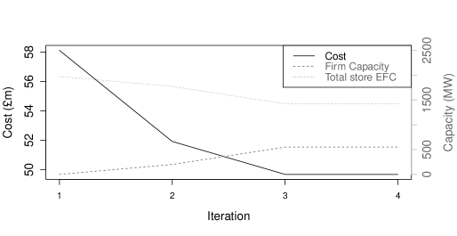
Figure 2: Iterative procedure: total market cost and associated capacity mix at the end of successive iterations.

Convergence to a set of resources $R$ such that (11) and (12) are then satisfied for the associated clearing price $p$ is obtained after three iterations—as confirmed by a fourth. Recall that, subject to the continuity and smoothness conditions of Section 2, these conditions are necessarily satisfied at the optimal set $R$, and—as argued in Section 4—might reasonably be expected to identify it uniquely. However, to the extent that capacity offerings in the market are discrete, absolute optimality cannot be guaranteed. (The final set of resources obtained here is identical with that obtained by the slower, simpler algorithm also discussed above.) The solution obtained—the set of resources $R$ meeting the required reliability standard at minimum cost on a pay-as-clear basis—is a combination of 550 MW of firm capacity and a set of stores the sum of whose EFCs $\mathit{efc}_{R}(i)$ evaluated with respect to $R$ is 1134 MW. These are the EFCs appropriate to the marginal contributions of the individual stores at the point where the market clears (and as is appropriate to the optimal operation of the capacity market—see Section 4), and determine their payments received in the capacity market. However, the EFC of the entire set of accepted stores—treated as a single unit—is 1423 MW, i.e. this is the amount of further firm capacity which would be required to substitute for the entire set of accepted stores in order to meet the required EEU reliability standard. (The total power rating of these stores is 3700 MW, but the store durations are quite low.) This is an extreme case of the nonadditivity of EFCs over significant numbers of resources, as discussed at the end of Section 4. It is further a reflection of the observation, at the end of Section 3, that the EFC of further storage resources is typically reduced by the presence of existing storage resources. A similar phenomenon is well known in the case of some variable generation such as wind power, although the reason for the latter is very different and results from the temporal coincidence of wind resources at different locations.

In GB (and other countries) the capacity market is settled through a single-pass descending-clock auction which identifies the required clearing price. Thus the EFCs of storage facilities—which now participate in the GB capacity market—are estimated in advance of the capacity auction. The EFC $\mathit{efc}_{R}(i)$ of each store $i$ is determined as described in the present paper, but—as for the first iteration of the present example—is done so with respect to an “initial” set of resources $R$ which is taken to be the amount of firm capacity which would be required in order to meet the GB reliability standard. In GB most resource currently participating in the market is conventional generation, and the storage EFCs estimated as above are close to their true values, i.e. to those calculated with respect to the set of resources $R$ finally obtained in the market. However, the example of the present section is chosen so that storage plays a significant role—something which may very well also be the case in future real systems. In this example the initial EFC estimates $\mathit{efc}_{R}(i)$ of the stores, determined as described above, prove to be considerable overestimates in comparison with their true values. The reason for this is as discussed at the end of Section 3: storage added to existing storage is less valuable than when added to firm capacity providing the same level of reliability. A consequence, in the present example, of this overvaluation of the contribution of storage would be that, if uncorrected, all the resource obtained in the capacity market would consist of storage—as at the end of the first iteration. Further, with the realistic resource costs chosen for this example, the cost of obtaining sufficient (all storage) resources to correctly meet the required reliability standard is £58.1m, whereas the true cost of the optimal resource set (as identified earlier and consisting of a mixture of firm capacity and storage) to meet that reliability standard is £49.7m. The more careful evaluation of the contribution of storage in the present example therefore leads to a cost saving of 14.5%.

Finally we test more carefully the extent to which the continuity and smoothness assumptions of Section 2 are applicable in the current example. Figure 3 shows the effect of starting with the background system of pre-existing capacity and gradually adding to it all the capacity-providing resources competing in the auction, taken in the order of the final merit-order stack. The figure plots residual EEU against cumulative EFC. At each point the latter is again the firm capacity which would substitute for the resources added so far while maintaining the same level of residual EEU (so that the underlying relationship defined by the plotted points is in fact independent of the order in which the resources are taken). We see that, as required for the continuity assumption, there are no large gaps between successive points. In particular these points are dense in the region corresponding to the target EEU for the auction—as represented by the horizontal line. We therefore conclude that the continuity assumption is sufficiently well satisfied.

Figure 3: Plot of residual EEU again cumulative EFC.

Figure 4 examines the validity of the smoothness assumption (3). It shows, as a “heat plot”, the percentage variation

$$\frac{\rho(R+i+j)-\rho(R+j)-(\rho(R+i)-\rho(R))}{\rho(R+i)-\rho(R)}\times 100\%$$

between the left and right sides of (3), where the set $R$ is taken to be the set of resources identified by the capacity auction and where the $x$- and $y$-axes give respectively the powers of the additional stores $i$ and $j$. These additional stores all have capacities of 100 MWh energy and levels of power which vary from $10$ to $50$ MW. The lowest powered stores contribute only modest additional capacity, and here (3) is seen to be very accurate. The highest powered stores contribute substantial additional capacity; nevertheless here the difference between the left and right sides of (3) is at most $5\%$. Similar results would be obtained if the additional resources $i$ and $j$ corresponded to firm capacity or conventional generation. The smoothness assumption therefore also appears sufficiently well satisfied here.

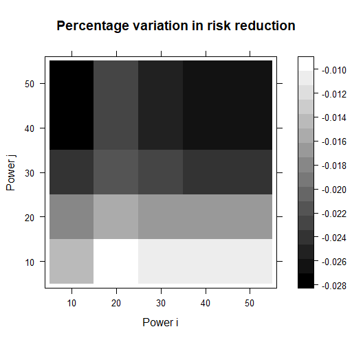
Figure 4: Heat plot to examine the accuracy of the smoothness assumption (3).

7 Conclusions

We have given a general theory to show how to value both variable generation and storage so as to enable them to be integrated fairly and optimally into electricity capacity markets, whether the objective within such a market is the optimal satisfaction of some security-of-supply metric or of some appropriate economic criterion. We have also considered the consequences for the practical operation of such markets. Storage, in particular, provides considerable challenges. We have argued that an appropriate risk metric is EEU rather than LOLE, shown how to calculate the latter for storage, and shown how to value its economic contribution. The EFC of storage is sensitive to the amount of storage already in the system to which it is being added, and this has considerable consequences for the fair and optimal operation of markets, as we demonstrate in a realistic practical example based on the current GB system (in which both conventional generation and storage—but not currently variable generation—participate).

Appendix: technical results

In this appendix we formalise and prove two technical results in the present paper.

Proof of equation (9).

We prove the result given by equation (9), namely that for any set of capacity-providing resources $R$ which consists entirely of generation, either conventional or variable, we have that the derivative $\mathrm{EEU}^{\prime}(R)$ of $\mathrm{EEU}(R)$ with respect to variation of firm capacity is given by $-\mathrm{LOLE}(R)$.

For each time $t$ let the random variable $Z_{t}$ be the supply-demand balance at time $t$ corresponding to the use of the set of resources $R$. Then, from (2), for any addition to $R$ of firm capacity equal to $\delta$,

$$\mathrm{EEU}(R+\delta)=\sum_{t=1}^{n}\int_{-\infty}^{0}\mathbf{P}(Z_{t}+\delta<z)\,dz=\sum_{t=1}^{n}\int_{-\infty}^{-\delta}\mathbf{P}(Z_{t}<z)\,dz,$$

so that, differentiating with respect to $\delta$ and then setting $\delta=0$, we have

$$\mathrm{EEU}^{\prime}(R)=-\sum_{t=1}^{n}\mathbf{P}(Z_{t}<0)=-\mathrm{LOLE}(R)$$

from (1) as required.

Proof of Proposition 1.

For any possible risk level $k$ of EEU, define $R_{k}$ to be the set of resources $R$ which minimises the cost $c(R)$ subject to the constraint $\mathrm{EEU}(R)=k$. Given the risk level $k$, the subproblem of determining $R_{k}$ is the problem considered in Section 4. The additional problem in the minimisation of the overall economic cost (13) may therefore be viewed as that of determining the value of $k$ such that $R_{k}$ minimises

$$\mathrm{VOLL}\times\mathrm{EEU}(R_{k})+c(R_{k}),$$ (16)

(with $\mathrm{EEU}(R_{k})=k$) i.e. that of determining the optimal level of EEU to be then obtained at minimum cost. We may consider the effect of infinitesimal variation of the risk level $k$ by considering the corresponding required infinitesimal variation in EFC, where the latter is defined with respect to $R_{k}$. At that value of $k$ such that the overall economic cost (16) is minimised, we have stationarity with respect to such variation, so that at this value of $k$, analogously to (14),

$$\mathrm{VOLL}\times\mathrm{EEU}^{\prime}(R_{k})+c^{\prime}(R_{k})=0,$$ (17)

where it follows from the definition of EFC in Section 3 that $\mathrm{EEU}^{\prime}(R_{k})$ may continue to be interpreted as defined in that section, i.e. as the derivative of $\mathrm{EEU}(R_{k})$ with respect to firm capacity, and where $c^{\prime}(R_{k})$ may similarly continue to be interpreted as the cost of new entry ($\mathrm{CONE}$) at the level of resource defined by $R_{k}$. Since it is assumed that all capacity-providing resource consists of some form of generation, the result (9) holds and so, analogously to (15), it follows that at the value of $k$ such that the overall cost (13) is minimised,

$$\mathrm{LOLE}(R_{k})=\frac{\mathrm{CONE}}{\mathrm{VOLL}}.$$ (18)

Now, for each $k$, recall the above definition of $R_{k}$. It follows from the assumed one-one correspondence between values of $\mathrm{EEU}(R)$ and those of $\mathrm{LOLE}(R)$ that $R_{k}$ is also the set of resources $R$ which minimises $c(R)$ subject to the corresponding constraint on $\mathrm{LOLE}(R)$. It thus follows from (18) that, exactly as in the case where all resource is provided by firm capacity only, the determination of the optimal set of capacity-providing resources minimising the overall economic cost (13) is again given by the minimisation of the cost $c(R)$ subject to the constraint (15).

References

- [1] R. Billinton and R.. Allan “Reliability Evaluation of Power Systems” Plenum, 1996
- [2] C. Bothwell and B.. Hobbs “Crediting Wind and Solar Renewables in Electricity Capacity Markets: The Effects of Alternative Definitions upon Market Efficiency” In The Energy Journal 38.1, 2017, pp. 173–188 DOI: 10.5547/01956574.38.SI1.cbot
- [3] J. Bowring “Capacity Markets in PJM” In Economics of Energy and Environmental Policy 2.2, 2013, pp. 47–64
- [4] J.. Cruise and S. Zachary “Optimal scheduling of energy storage resources”, 2018 URL: http://arxiv.org/abs/1808.05901
- [5] C.. Dent and S. Zachary “Further results on the probability theory of capacity value of additional generation” In 2014 International Conference on Probabilistic Methods Applied to Power Systems (PMAPS), 2014, pp. 1–6 DOI: 10.1109/PMAPS.2014.6960667
- [6] Department of Energy and Climate Change “EMR Consultation Annex C: Reliability Standard Methodology” Accessed 30 June 2021, 2013 URL: https://assets.publishing.service.gov.uk/government/uploads/system/uploads/attachment_data/file/223653/emr_consultation_annex_c.pdf
- [7] G. Edwards, S. Sheehy, C.. Dent and M… Troffaes “Assessing the contribution of nightly rechargeable grid-scale storage to generation capacity adequacy” In Sustainable Energy, Grids and Networks 12 Elsevier, 2017, pp. 69–81 DOI: 10.1016/J.SEGAN.2017.09.005
- [8] M. Evans, S.. Tindemans and D. Angeli “Robustly Maximal Utilisation of Energy-Constrained Distributed Resources” In 2018 Power Systems Computation Conference (PSCC), 2018, pp. 1–7 DOI: 10.23919/PSCC.2018.8443058
- [9] J. Geske and R. Green “Optimal Storage, Investment and Management under Uncertainty: It is Costly to Avoid Outages!” In The Energy Journal 41.2, 2020, pp. 1–27 DOI: 10.5547/01956574.41.2.jges
- [10] D. Helm “Cost of energy: independent review” Accessed 30 June 2021, 2017 URL: https://www.gov.uk/government/publications/cost-of-energy-independent-review
- [11] B. Hobbs et al. “A Dynamic Analysis of a Demand Curve-Based Capacity Market Proposal: The PJM Reliability Pricing Model” In IEEE Transactions on Power Systems 22.1, 2007, pp. 3–14 DOI: 10.1109/TPWRS.2006.887954
- [12] P. Holmberg and R.. Ritz “Optimal Capacity Mechanisms for Competitive Electricity Markets” In The Energy Journal 41.SI1, 2021, pp. 33–66 DOI: 10.5547/01956574.42.S12.phol
- [13] ISO New England “FCM Primary Auction Mechanics” Accessed 30 June 2021, 2020 URL: https://www.iso-ne.com/markets-operations/markets/forward-capacity-market/fcm-participation-guide/fcm-auction-mechanics
- [14] A. Keane et al. “Capacity Value of Wind Power” In IEEE Transactions on Power Systems 26.2, 2011, pp. 564–572 DOI: 10.1109/TPWRS.2010.2062543
- [15] F. Lopes and H. Algarvio “Demand Response in Electricity Markets: An Overview and a Study of the Price-Effect on the Iberian Daily Market” In Electricity Markets with Increasing Levels of Renewable Generation: Structure, Operation, Agent-based Simulation, and Emerging Designs Springer, 2018, pp. 265–303 DOI: 10.1007/978-3-319-74263-2˙10
- [16] R.. Moye and S.. Meyn “Redesign of US Electricity Capacity Markets” In Energy Markets and Responsive Grids: Modeling, Control, and Optimization Springer, 2018, pp. 73–103 DOI: 10.1007/978-1-4939-7822-9
- [17] National Grid plc “Capacity Auction User Guide” Accessed 30 June 2021, 2016 URL: https://www.emrdeliverybody.com/Lists/Latest%20News/Attachments/72/Auction%20Guidance%20v1.pdf
- [18] National Grid plc “Capacity Market Auction Guidelines” Accessed 30 June 2021, 2018 URL: https://www.emrdeliverybody.com/Lists/Latest%20News/Attachments/197/Auction%20Guidelines%202018%20v2.0.pdf
- [19] National Grid plc “Electricity Capacity Report” Accessed 30 June 2021, 2018 URL: https://www.emrdeliverybody.com/Capacity%20Markets%20Document%20Library/Electricity%20Capacity%20Report%202018.pdf
- [20] National Grid plc “Capacity Market: The Demand Curve” Accessed 30 June 2021, 2020 URL: https://www.emrdeliverybody.com/CM/The-Demand-Curve.aspx
- [21] D… Newbery “Missing money and missing markets: Reliability, capacity auctions and interconnectors” In Energy Policy 94, 2015, pp. 401–410 DOI: 10.1016/j.enpol.2015.10.028
- [22] Ofgem “Wholesale Energy Markets in 2016” Accessed 30 June 2021, 2016 URL: https://www.ofgem.gov.uk/system/files/docs/2016/08/wholesale_energy_markets_in_2016.pdf
- [23] I. Staffell and R. Green “Is There Still Merit in the Merit Order Stack? The Impact of Dynamic Constraints on Optimal Plant Mix” In IEEE Transactions on Power Systems 31.1, 2016, pp. 43–53 DOI: 10.1109/TPWRS.2015.2407613
- [24] S. Stoft “Power System Economics: Designing Markets for Electricity” IEEE/Wiley, 2002
- [25] A.. Wilson, S. Zachary and C.. Dent “Use of meteorological data for improved estimation of risk in capacity adequacy studies” In 2018 International Conference on Probabilistic Methods Applied to Power Systems (PMAPS), 2018, pp. 1–6 DOI: 10.1109/PMAPS.2018.8440216
- [26] S. Zachary and C.. Dent “Probability theory of capacity value of additional generation” In Proceedings of the Institution of Mechanical Engineers, Part O: Journal of Risk and Reliability 226.1, 2011, pp. 33–43 DOI: 10.1177/1748006X11418288
- [27] F. Zhao, T. Zheng and E. Litvinov “Constructing Demand Curves in Forward Capacity Market” In IEEE Trans. Power Syst. 33.1, 2018, pp. 525–535 DOI: 10.1109/TPWRS.2017.2686785