Characterising random partitions by random colouring

Abstract.

Let $(X_{1},X_{2},...)$ be a random partition of the unit interval $[0,1]$, i.e. $X_{i}\geq 0$ and $\sum_{i\geq 1}X_{i}=1$, and let $(\varepsilon_{1},\varepsilon_{2},...)$ be i.i.d. Bernoulli random variables of parameter $p\in(0,1)$. The Bernoulli convolution of the partition is the random variable $Z=\sum_{i\geq 1}\varepsilon_{i}X_{i}$. The question addressed in this article is: Knowing the distribution of $Z$ for some fixed $p\in(0,1)$, what can we infer about the random partition $(X_{1},X_{2},...)$? We consider random partitions formed by residual allocation and prove that their distributions are fully characterised by their Bernoulli convolution if and only if the parameter $p$ is not equal to $\nicefrac{{1}}{{2}}$.

1. Introduction

Random partitions appear in the mathematical description of many natural systems, such as particle clustering and condensation in physics [4]; dynamics of gene populations in biology [9]; wealth distribution in economics [19]; etc. There is a vast amount of possible probability laws of random partitions, but one often encounters convergence to one of a few universal laws, most notably the Poisson–Dirichlet distribution with parameter $\theta>0$, henceforth denoted $\mathtt{PD}(\theta)$ and defined below after Eq. (1.5).

To show convergence of a tight sequence of random partitions it is often feasible to show convergence of a derived quantity like the Bernoulli convolutions studied in this paper. If the limit of the derived quantity characterises the law of the underlying random partition among the class of possible limits, convergence is shown. It is therefore an important question whether the distribution of a random partition can be identified from its Bernoulli convolution, and in this paper we contribute to this problem.

We describe two scenarios that motivate this study in Sections 1.1 and 1.2. We introduce the precise setting and our results in Section 1.3 — the definition of the Bernoulli convolution can be found around Eq. (1.4). Sections 2 and 3 contain the proofs of our two theorems. We make further comments in Section 4; it includes a counterexample due to A. Holroyd, that sheds much light on these questions.

1.1. Random interchange model and quantum spin systems

The random interchange model is a process on permutations constructed as products of random transpositions. Namely, given integers $n$ and $k$, we pick $k$ pairs of distinct integers $(x_{1},y_{1}),\dotsc,(x_{k},y_{k})$ from $\{1,\dotsc,n\}$ uniformly at random, and consider the permutation

$$\sigma=\tau_{k}\circ\dots\circ\tau_{1}.$$ (1.1)

Here, $\tau_{i}=(x_{i},y_{i})$ denotes the transposition of $x_{i}$ and $y_{i}$. The cycle structure (i.e. the lengths of the permutation cycles) of $\sigma$ gives an integer partition of $n$; dividing by $n$ gives a partition of $[0,1]$.

Schramm [18] studied this model in the case where $k=\lfloor cn\rfloor$ with $c>1$. He proved that, with high probability as $n\to\infty$, there are cycles whose lengths are of order $n$. Let $L_{i}$ denote the length of the $i$th largest cycle. The sum of cycles of length of order $n$ is $\kappa n(1+o(1))$ with $\kappa=\kappa(c)$ fixed (and $\kappa\to 1$ when $c\to\infty$); and the sequence $(\frac{L_{1}}{\kappa n},\frac{L_{2}}{\kappa n},\dots)$ converges (weakly) to $\mathtt{PD}(1)$, the Poisson–Dirichlet distribution with parameter 1.

One motivation for the random interchange model, pointed out and exploited by Tóth [21], is that it provides a probabilistic representation of the Heisenberg model of quantum spins. For this representation the density of the random interchange model gets an extra weight $2^{\#{\rm cycles}}$, which leads to a conjectured limit which is the Poisson–Dirichlet distribution $\mathtt{PD}(2)$, see [11]. In this case the number of transpositions $k$ is random, chosen to be $\mathtt{Poisson}(cn)$. Recently, it was proved in [6] that, in the model with weight $\theta^{\#{\rm cycles}}$, $\theta=2,3,4,\dots$, we have

$$\lim_{n\to\infty}{\mathbb{E}}_{n}\Bigl{[}\prod_{i\geq 1}\tfrac{1}{\theta}(\,{\rm e}^{hL_{i}/n}\,+\theta-1)\Bigr{]}=\,{\rm e}^{\frac{h}{\theta}(1-\kappa)}\,{\mathbb{E}}_{\mathtt{PD}(\theta)}\Bigl{[}\prod_{i\geq 1}\tfrac{1}{\theta}(\,{\rm e}^{h\kappa X_{i}}\,+\theta-1)\Bigr{]},$$ (1.2)

for some (deterministic) $\kappa\in[0,1]$ which depends on $c$ and $\theta$ and is positive for $c$ large enough; the above identity holds for all $h\in{\mathbb{C}}$. The last expectation in (1.2) is equal to the moment generating function at $h\kappa$ of the Bernoulli convolution of $\mathtt{PD}(\theta)$ with parameter $p=\nicefrac{{1}}{{\theta}}$. The interpretation is that the system displays small (order 1) and large (order $n$) cycles, and that the joint distribution of the lengths of large cycles is $\mathtt{PD}(\theta)$; see [6] for more details. But is Eq. (1.2) enough to guarantee that the limiting sequence of renormalised cycle lengths be equal to $\mathtt{PD}(\theta)$? We prove here that, among the residual allocation distributions, the answer is yes for $\theta=3,4,\dots$, but no for $\theta=2$.

There are related loop models that include ‘double bars’ as well as the transposition ‘crosses’, that represent further quantum spin systems [2, 22]. Without weights, it was proved in [7] that the joint distribution of the lengths of long loops is $\mathtt{PD}(\nicefrac{{1}}{{2}})$. With weights $2^{\#{\rm loops}}$, the result of [6] is that

$$\lim_{n\to\infty}{\mathbb{E}}_{n}\Bigl{[}\prod_{i\geq 1}\cos(hL_{i}/n)\Bigr{]}={\mathbb{E}}_{\mathtt{PD}(1)}\Bigl{[}\prod_{i\geq 1}\cos(h\kappa X_{i})\Bigr{]},$$ (1.3)

for all $h\in{\mathbb{C}}$. The latter expectation is closely related to the moment generating function of the Bernoulli convolution of $\mathtt{PD}(1)$ with parameter $p=\nicefrac{{1}}{{2}}$. Results of the present article show that the above claim is not enough to guarantee that the limiting distribution is $\mathtt{PD}(1)$, even if one assumes that the limiting distribution is a residual allocation.

1.2. Exchangeable divide-and-color models

In a recent paper by Steif and Tykesson [20], the authors introduce generalized divide-and-color models as follows. Given a countable set $S$ and $p\in(0,1)$, one starts by forming a random partition $\Pi$ of $S$ according to some rule; one then assigns to each part of $\Pi$ a ‘color’ 0 or 1, independently and with probability $p$ for 1. Letting each element of $S$ take the color of the part it belongs to and then forgetting about the original parition $\Pi$, one ends up with a random element $\omega\in\{0,1\}^{S}$. This construction is motivated by the Fortuin–Kasteleyn representation of the Ising model, among other examples.

A particular case is when $S={\mathbb{N}}$ and when the random partition $\Pi$ is exchangeable, i.e. its distribution is invariant under all finite permutations of ${\mathbb{N}}$. By Kingman’s famous theorem [13], such a random partition of ${\mathbb{N}}$ is uniquely encoded by a random vector $(X_{i})_{i\geq 1}$ satisfying $X_{i}\geq X_{i+1}\geq 0$ for all $i\geq 1$ and $\sum_{i\geq 1}X_{i}\leq 1$; note that $<1$ is allowed in this case. On the other hand, the resulting color process $\omega\in\{0,1\}^{\mathbb{N}}$ is also exchangeable; by de Finetti’s theorem, this means that there is some random variable $\xi\in[0,1]$ such that, conditional on $\xi$, the $\omega_{i}$ are i.i.d. $\mathtt{Bernoulli(\xi)}$. It is not hard to see that (when $\sum_{i\geq 1}X_{i}=1$) $\xi$ equals the Bernoulli convolution of $(X_{i})_{i\geq 1}$, see [20, Lemma 3.12]. Steif and Tykesson ask whether the law of the random partition $\Pi$ can be recovered from the law of $\omega$ when $p\neq\nicefrac{{1}}{{2}}$. This is equivalent to asking whether the law of $(X_{i})_{i\geq 1}$ can be recovered from the law of its Bernoulli convolution. Our results on residual allocation models show that the answer can be yes under additional assumptions on $(X_{i})_{i\geq 1}$.

1.3. Framework and results

We define a Bernoulli convolution as follows.

Definition.

Let $(X_{i})_{i\geq 1}$ be a random partition of $[0,1]$, i.e. $X_{i}\geq 0$ for all $i\geq 1$ and $\sum_{i\geq 1}X_{i}=1$. Let $({\varepsilon}_{i})_{i\geq 1}$ be a sequence of i.i.d. Bernoulli random variables of parameter $p\in(0,1)$, independent of $(X_{i})_{i\geq 1}$. Set

$$Z=\sum_{i\geq 1}{\varepsilon}_{i}X_{i}.$$ (1.4)

The law of $Z$, and sometimes the random variable $Z$ itself, is called the Bernoulli($p$) convolution of the random partition $(X_{i})_{i\geq 1}$.

We restrict our setting to random partitions obtained from residual allocation. Namely, we consider the interval $[0,1]$ with the Borel $\sigma$-algebra. Given a probability measure $\mu$ on $[0,1]$, let $(Y_{i})_{i\geq 1}$ be i.i.d. random variables distributed according to $\mu$, and consider the sequence $(X_{i})_{i\geq 1}$ defined by

$$\begin{split}&X_{1}=Y_{1},\\ &X_{2}=(1-Y_{1})Y_{2},\\ &X_{3}=(1-Y_{1})(1-Y_{2})Y_{3},\\ &\text{etc...}\end{split}$$ (1.5)

Assuming that $\mu(\{0\})<1$, it is not hard to prove that $X_{i}\to 0$ as $i\to\infty$ and that $\sum_{i\geq 1}X_{i}=1$, almost surely. It is possible to rearrange the sequence $(X_{i})_{i\geq 1}$ in decreasing order if one wants an ordered partition, but this is not necessary here.

An important example of this construction is the Griffiths, Engen and McCloskey distribution, $\mathtt{GEM}(\theta)$, obtained when $\mu=\mathtt{Beta}(1,\theta)$. If one orders the entries of a $\mathtt{GEM}(\theta)$ sample by decreasing size, one obtains the famous Poisson–Dirichlet distribution $\mathtt{PD}(\theta)$, see [12]. Another important example is the ‘classical’ Bernoulli convolution $\sum_{i\geq 1}\pm\lambda^{i}$ with i.i.d. random signs; see the review [14]. This falls into our framework (take $\mu=\delta_{1-\lambda}$ for some fixed $\lambda\in(0,1)$ so that $X_{i}=(1-\lambda)\lambda^{i-1}$), except that our Bernoulli coefficients take value in $\{0,1\}$ instead of $\{-1,1\}$.

As a shorthand, since we only consider random partitions from residual allocation, we will sometimes refer to $Z$ (or its law) as the Bernoulli convolution of the measure $\mu$. The Bernoulli convolution is invariant under rearrangements of the sequence $(X_{i})_{i\geq 1}$. The cases $p=0$ and $p=1$ are trivial and uninteresting, since $Z=0$ and $Z=1$, respectively.

If $\mu$ has an atom at 0 of value $c>0$, i.e. $\mu(\{0\})=c$, then the sequence $(Y_{1},Y_{2},\dots)$ — and therefore $(X_{1},X_{2},\dots)$ — contains a density $c$ of elements that are equal to 0; this does not affect $Z$. In other words, the Bernoulli convolutions of $\mu$ and $c\delta_{0}+(1-c)\mu$ are the same for all $c\in[0,1)$. We avoid this trivial degeneracy by restricting our attention to measures that do not have an atom at 0.

Given $p\in(0,1)$, the question is whether the Bernoulli($p$) convolution characterises the random partition obtained from residual allocation. We show that it is the case for $p\neq\nicefrac{{1}}{{2}}$.

Theorem 1.1.

Let $p\in(0,1)\setminus\{\nicefrac{{1}}{{2}}\}$. If $\mu$ and $\nu$ are two probability measures on $[0,1]$ such that $\mu(\{0\})=\nu(\{0\})=0$, and the corresponding residual allocation models have identical Bernoulli($p$) convolution, then $\mu=\nu$.

We also show that Theorem 1.1 fails for $p=\nicefrac{{1}}{{2}}$. Our non-uniqueness results hold for $\mathtt{GEM}$ (or Poisson–Dirichlet) measures of arbitrary parameters.

Theorem 1.2.

Let $\theta>0$ and $\mu=\mathtt{Beta}(1,\theta)$. Then there exist infinitely many $\nu\neq\mu$ such that $\nu(\{0\})=0$, and such that $\mu$ and $\nu$ have identical Bernoulli($\nicefrac{{1}}{{2}}$) convolutions.

The non-uniqueness results are not explicit with the exception of $\mathtt{GEM}(2)$: We show that if an (absolutely continuous) measure $\nu$ satisfies

$$x\,{\rm d}\nu(x)=(1-x)\,{\rm d}\nu(1-x)\quad\text{ for all }x\in[0,1],$$ (1.6)

then its residual allocation has the same Bernoulli convolution as $\mu=\mathtt{Beta}(1,2)$. Note that (1.6) holds true in the case $\mu=\mathtt{Beta}(1,2)$, for which ${\rm d}\mu(x)=2(1-x){\rm d}x$. Another example is the Dirac measure at $x=\nicefrac{{1}}{{2}}$, $\nu=\delta_{\nicefrac{{1}}{{2}}}$, which formally satisfies (1.6). We refer to Proposition 3.4 for details including conditions on the regularity of measures.

We prove Theorems 1.1 and 1.2 with the help of a stochastic identity for the random variable $Z$, see Lemma 2.1. This identity holds because of the self-similarity structure of residual allocations. The proofs of Theorem 1.1 and 1.2 can be found in Sections 2 and 3, respectively.

A natural question is whether Theorem 1.1 holds beyond residual allocations. Obviously, the Bernoulli convolution (1.4) may be defined for arbitrary random partitions $(X_{i})_{i\geq 1}$. Alexander Holroyd has given an example showing that, in general, the Bernoulli convolution does not determine the random partition, even if the former is known for all $p\in(0,1)$; we explain Holroyd’s example in Section 4. One may also allow more general random variables $({\varepsilon}_{i})_{i\geq 1}$; in this generality, $Z$ is sometimes called a random weighted average. Pitman’s recent review [15] contains a wealth of information about the theory of random weighted averages. In [15, Corollary 9] it is shown that the distributions of the random weighted averages $Z$, as $({\varepsilon}_{i})_{i\geq 1}$ range over all i.i.d. sequences of random variables with finite support, fully characterize the law of the random partition $(X_{i})_{i\geq 1}$. This holds without any assumptions about the properties of the random partition. It is natural to ask whether the condition on the ${\varepsilon}_{i}$ can be weakened.

2. Uniqueness when $p\neq\nicefrac{{1}}{{2}}$ (proof of Theorem 1.1)

The following lemma will be used both to establish uniqueness for $p\neq\nicefrac{{1}}{{2}}$ and non-uniqueness for $p=\nicefrac{{1}}{{2}}$.

Lemma 2.1.

Let $Y,Y_{1},Y_{2},\dots$ be i.i.d. random variables with values in $[0,1]$ and $(X_{i})_{i\geq 1}$ defined by (1.5); ${\varepsilon},{\varepsilon}_{1},{\varepsilon}_{2},\dots$ be i.i.d. $\mathtt{Bernoulli}(p)$ random variables independent of the $Y$’s; and $Z$ and $Z^{\prime}$ be two identically distributed random variables with values in $[0,1]$, $Z^{\prime}$ being independent of $Y$ and ${\varepsilon}$. The following stochastic identities are equivalent:

• $\displaystyle Z\overset{\rm d}{=}\sum_{i\geq 1}{\varepsilon}_{i}X_{i}$;

• $\displaystyle Z\overset{\rm d}{=}{\varepsilon}Y+(1-Y)Z^{\prime}$.

This is not new, see [10, Theorem 1] or [8, Theorem 7.1]; it is also discussed in [15, (119)].

Proof.

Assuming $(a)$, we have

$$Z\overset{\rm d}{=}{\varepsilon}_{1}Y_{1}+(1-Y_{1})\sum_{i\geq 2}{\varepsilon}_{i}\frac{X_{i}}{1-Y_{1}},$$

where the sequence $(X_{i}/(1-Y_{1}))_{i\geq 2}$ is independent of $X_{1}=Y_{1}$ and has the same distribution as $(X_{i})_{i\geq 1}$, which gives (b).

Assuming $(b)$, we construct a sequence of random variables which all have the same distribution as $Z$ and which converge weakly (in fact, almost surely) to $\sum_{i\geq 1}{\varepsilon}_{i}X_{i}$. Observe that there exist $Z_{1}$ and $Z_{2}$ two independent copies of $Z$, independent of ${\varepsilon}_{i}$ and $Y_{i}$ such that

$$\begin{split}Z_{1}&\overset{\rm d}{=}{\varepsilon}_{1}Y_{1}+(1-Y_{1})Z_{1}\\ &\overset{\rm d}{=}{\varepsilon}_{1}Y_{1}+(1-Y_{1})\bigl{[}{\varepsilon}_{2}Y_{2}+(1-Y_{2})Z_{2}\bigr{]}.\end{split}$$ (2.1)

Iterating this further, we get $(Z_{i})_{i\geq 1}$ such that for all $n\geq 1$,

$$\sum_{i=1}^{n}{\varepsilon}_{i}X_{i}+(1-Y_{1})\dotsb(1-Y_{n})Z_{n}\overset{\rm d}{=}Z_{1},$$ (2.2)

where $X_{i}$ are as defined in (1.5). All terms in $\sum_{i=1}^{n}{\varepsilon}_{i}X_{i}$ are positive and the sums are bounded by 1, hence the series converges to $\sum_{i\geq 1}{\varepsilon}_{i}X_{i}$; the remainder $(1-Y_{1})\dotsb(1-Y_{n})Z_{n}$ converges to 0 almost surely. As $n\to\infty$ we obtain (a). ∎

We will show that all moments of $Y\sim\mu$ are determined by the Bernoulli convolution $Z$ of the residual allocation model from $\mu$. This holds for $p\in(0,1)\setminus\{\nicefrac{{1}}{{2}}\}$. It does not hold for $p=0$ (the Bernoulli convolution is always 0) and $p=1$ (it is always 1). It also does not hold for $p=\nicefrac{{1}}{{2}}$, for reasons that are not obvious and that are discussed in Sect. 3.

Let us introduce numbers $a_{n,k}$ and $c_{n}$ that depend on the law of $Z$, and numbers $b_{n}$ that depend on the law of $Y$. For $n,k\in{\mathbb{N}}$ with $k\leq n$, let

$$\begin{split}&a_{n,k}=(-1)^{k}p\binom{n}{k}{\mathbb{E}}\bigl{[}(1-Z)^{k}\bigr{]},\\ &c_{n}=(1-p){\mathbb{E}}[Z^{n}],\\ &b_{n}=\frac{1-{\mathbb{E}}\bigl{[}(1-Y)^{n}\bigr{]}}{{\mathbb{E}}[Y]}.\end{split}$$ (2.3)

Note that $b_{0}=0$, $b_{1}=1$, and $a_{1,1}+c_{1}=0$ since ${\mathbb{E}}[Z]=p$. We have the following relations.

Proposition 2.2.

For all $p\in[0,1]$ and all $n\geq 1$, we have

$$c_{n}b_{n}+\sum_{k=1}^{n}a_{n,k}b_{k}=0.$$

Proof.

We expand ${\mathbb{E}}[Z^{n}]$ in two different ways. First,

$$\begin{split}{\mathbb{E}}[Z^{n}]&=(1-p){\mathbb{E}}[Z^{n}]+p{\mathbb{E}}\bigl{[}\bigl{(}1-(1-Z)\bigr{)}^{n}\bigr{]}\\ &=(1-p){\mathbb{E}}[Z^{n}]+p\sum_{k=0}^{n}(-1)^{k}\binom{n}{k}{\mathbb{E}}\bigl{[}(1-Z)^{k}\bigr{]}.\end{split}$$ (2.4)

Second, using Lemma 2.1,

$$\begin{split}\mathbb{E}[Z^{n}]&=\mathbb{E}\bigl{[}\big{(}{\varepsilon}Y+(1-Y)Z\big{)}^{n}\bigr{]}=p\mathbb{E}\bigl{[}\big{(}Y+(1-Y)Z\big{)}^{n}\bigr{]}+(1-p)\mathbb{E}\bigl{[}\big{(}(1-Y)Z\big{)}^{n}\bigr{]}\\ &=(1-p)\mathbb{E}\bigl{[}(1-Y)^{n}\bigr{]}\mathbb{E}[Z^{n}]+p\mathbb{E}\bigl{[}\big{(}1-(1-Y)(1-Z)\big{)}^{n}\bigr{]}\\ &=(1-p)\mathbb{E}\bigl{[}(1-Y)^{n}\bigr{]}\mathbb{E}[Z^{n}]+p\sum_{k=0}^{n}(-1)^{k}\binom{n}{k}\mathbb{E}\bigl{[}(1-Y)^{k}\bigr{]}\mathbb{E}\bigl{[}(1-Z)^{k}\bigr{]}.\end{split}$$ (2.5)

Equating these identities, we get

$$0=(1-p){\mathbb{E}}[Z^{n}]\bigl{\{}1-{\mathbb{E}}\bigl{[}(1-Y)^{n}\bigr{]}\bigr{\}}+p\sum_{k=0}^{n}(-1)^{k}\binom{n}{k}{\mathbb{E}}\bigl{[}(1-Z)^{k}\bigr{]}\bigl{\{}1-{\mathbb{E}}\bigl{[}(1-Y)^{k}\bigr{]}\bigr{\}}.$$ (2.6)

We now divide by ${\mathbb{E}}[Y]$ and we obtain the claim of the proposition. ∎

The next lemma holds for $p\neq\nicefrac{{1}}{{2}}$ only.

Lemma 2.3.

For $p\in(0,1)\setminus\{\nicefrac{{1}}{{2}}\}$, we have for all $n\geq 2$ that

$$a_{n,n}+c_{n}\neq 0.$$

Proof.

We have

$$a_{n,n}+c_{n}=(1-p)\mathbb{E}[Z^{n}]+(-1)^{n}p\mathbb{E}\bigl{[}(1-Z)^{n}\bigr{]}.$$ (2.7)

This is always positive for $n$ even; we thus assume from now on that $n\geq 3$ is odd. From the definitions (1.5) and (1.4), we have

$$\mathbb{E}[Z^{n}]=\sum_{i_{1},i_{2},\dotsc,i_{n}\geq 1}\mathbb{E}\big{[}{\varepsilon}_{i_{1}}{\varepsilon}_{i_{2}}\dotsb{\varepsilon}_{i_{n}}\big{]}\mathbb{E}\big{[}X_{i_{1}}X_{i_{2}}\dotsb X_{i_{n}}\big{]}.$$ (2.8)

Note that, if $\ell=\#\{i_{1},\dotsc,i_{n}\}$ denotes the number distinct indices among $i_{1},\dotsc,i_{n}\geq 1$, then

$$\mathbb{E}\big{[}{\varepsilon}_{i_{1}}{\varepsilon}_{i_{2}}\dotsb{\varepsilon}_{i_{n}}\big{]}=p^{\ell},$$ (2.9)

since ${\varepsilon}_{i}^{k}={\varepsilon}_{i}$ for all $k,i\geq 1$. We thus get

$$\mathbb{E}[Z^{n}]=\sum_{\ell=1}^{n}p^{\ell}\mathbb{E}[S_{n,\ell}],$$ (2.10)

where $S_{n,\ell}=\sum X_{i_{1}}X_{i_{2}}\dotsb X_{i_{n}}$ summed over all choices of indices $i_{1},\dotsc,i_{n}\geq 1$ such that $\#\{i_{1},\dotsc,i_{n}\}=\ell$. Note that $\mathbb{E}[S_{n,\ell}]>0$ for all $\ell\geq 1$. Since, by definition, $1-Z=\sum_{i\geq 1}(1-{\varepsilon}_{i})X_{i}$ we also have $\mathbb{E}[(1-Z)^{n}]=\sum_{\ell=1}^{n}(1-p)^{\ell}\mathbb{E}[S_{n,\ell}]$, and thus

$$a_{n,n}+c_{n}=p(1-p)\,\mathbb{E}[S_{n,\ell}]\,\sum_{\ell=1}^{n}\bigl{(}p^{\ell-1}-(1-p)^{\ell-1}\bigr{)}.$$ (2.11)

While the term $\ell=1$ is zero, all other terms are non-zero and have the same sign, which proves the claim since $n>1$. ∎

We now turn to the proof of Theorem 1.1.

Proof of Theorem 1.1.

It follows from Proposition 2.2 and Lemma 2.3 that, for $n\geq 2$,

$$b_{n}=-(a_{n,n}+c_{n})^{-1}\sum_{k=1}^{n-1}a_{n,k}b_{k}.$$ (2.12)

Recall that $b_{0}=0$, $b_{1}=1$. The above equation shows that the $b_{n}$’s are recursively determined by the $a_{n,k}$’s and $c_{n}$’s, which only depend on the Bernoulli convolution $Z$. As $n\to\infty$, the sequence $(b_{n})$ converges to $1/{\mathbb{E}}[Y]$ — here we use our assumption that the measure $\mu$ does not have an atom at $0$. It follows that ${\mathbb{E}}[Y]$ and ${\mathbb{E}}[(1-Y)^{n}]$ are determined by the Bernoulli convolution for all $n$. Then all moments of the original measure $\mu$ are known, hence the measure $\mu$ itself (see [5, Theorem 1.2]). ∎

3. Non-uniqueness when $p=\nicefrac{{1}}{{2}}$ (proof of Theorem 1.2)

In this section we set $p=\nicefrac{{1}}{{2}}$, unless indicated otherwise. We also assume that the Bernoulli convolution of parameter $\nicefrac{{1}}{{2}}$ has a density $q(x)$ with respect to Lebesgue measure, and that $q(x)>0$ for all $x\in(0,1)$. This will hold in particular in the case of $\mathtt{GEM}(\theta)$. Since $p=\nicefrac{{1}}{{2}}$ we then have that $q(x)=q(1-x)$ because $Z\overset{\rm d}{=}1-Z$.

Given a nonnegative measurable function $\rho$ on $[0,1]$, we define the function $H\rho$ by

$$[H\rho](x)=\frac{1}{q(x)}\int_{0}^{x}q\Bigl{(}\frac{x-u}{1-u}\Bigr{)}\frac{\rho(u)}{1-u}{\rm d}u.$$ (3.1)

Let ${\mathcal{R}}_{q}$ be the cone of nonnegative measurable functions $\rho$ such that the integral above is finite for all $0\leq x\leq 1$. $H$ is a linear operator on ${\mathcal{R}}_{q}$. As it turns out, it gives a relation between the density $\rho$ of a probability measure on $[0,1]$, and the density $q$ of the corresponding Bernoulli convolution. This may be seen by expanding the stochastic identity of Lemma 2.1 (b) and making a suitable change of variables. More precisely, we have:

Lemma 3.1.

Let $q$ be a probability density function on $[0,1]$ such that $q(x)>0$ on $(0,1)$ and $q(x)=q(1-x)$. Let $\rho\in{\mathcal{R}}_{q}$; we have

$$[H\rho](x)+[H\rho](1-x)=2,\quad\text{for almost all }x\in[0,1],$$ (3.2)

if and only if

• $\rho$ is a probability density function on $[0,1]$, and

• the Bernoulli($\nicefrac{{1}}{{2}}$) convolution of the residual allocation model from $\rho$ has density $q$.

Proof.

Assume that (3.2) holds. For (a), we have, writing $h(x)=[H\,\rho](x)$,

$$\begin{split}1&=\int_{0}^{1}q(x)\tfrac{h(x)+h(1-x)}{2}\,{\rm d}x=\int_{0}^{1}q(x)h(x)\,{\rm d}x=\int_{0}^{1}{\rm d}u\,\rho(u)\int_{u}^{1}{\rm d}z\tfrac{1}{1-u}q\big{(}\tfrac{z-u}{1-u}\big{)}\\ &=\int_{0}^{1}{\rm d}u\,\rho(u)\int_{0}^{1}{\rm d}v\,q(v)=\int_{0}^{1}{\rm d}u\,\rho(u),\end{split}$$ (3.3)

as claimed. (We used the change of variables $v=\tfrac{z-u}{1-u}$.)

For (b), we use (3.2) to get

$$q(x)=\tfrac{1}{2}\int_{0}^{x}q\Bigl{(}\frac{x-u}{1-u}\Bigr{)}\frac{\rho(u)}{1-u}{\rm d}u+\tfrac{1}{2}\int_{0}^{1-x}q\Bigl{(}\frac{x}{1-u}\Bigr{)}\frac{\rho(u)}{1-u}{\rm d}u.$$ (3.4)

It follows that for all continuous function $f$, we have

$$\begin{split}\int_{0}^{1}&q(x)f(x)\,{\rm d}x\\ &=\tfrac{1}{2}\int_{0}^{1}\frac{\rho(u)}{1-u}{\rm d}u\int_{u}^{1}q\Bigl{(}\frac{x-u}{1-u}\Bigr{)}f(x){\rm d}x+\tfrac{1}{2}\int_{0}^{1}\frac{\rho(u)}{1-u}{\rm d}u\int_{0}^{1-u}q\Bigl{(}\frac{x}{1-u}\Bigr{)}f(x){\rm d}x\\ &=\tfrac{1}{2}\int_{0}^{1}\rho(u){\rm d}u\int_{0}^{1}f\bigl{(}u+(1-u)y\bigr{)}q(y){\rm d}y+\tfrac{1}{2}\int_{0}^{1}\rho(u){\rm d}u\int_{0}^{1}f\bigl{(}(1-u)y\bigr{)}q(y){\rm d}y.\end{split}$$ (3.5)

We used Fubini’s theorem to get the second line, and the changes of variables $y=\frac{x-u}{1-u}$ and $y=\frac{x}{1-u}$ (for fixed $u$) to get the third line. The left side gives the expectation ${\mathbb{E}}[f(Z)]$ for the random variable with density $q$. The right side gives ${\mathbb{E}}[f({\varepsilon}Y+(1-Y)Z)]$ for the independent random variables ${\varepsilon}\sim\mathtt{Bernoulli}(\frac{1}{2})$, $Y$ with density $\rho$, and $Z$ with density $q$. We recognise the stochastic identity of Lemma 2.1 (b). Hence $q$ is the density of the Bernoulli convolution of $\rho$.

The other implication can be checked similarly: (3.5) holds by (b), hence also (3.4) for almost all $x$, which gives (3.2). ∎

The next step is to identify the Bernoulli convolution of $\mathtt{GEM}$ distributions. It turns out to be equal to Beta random variables. We consider general parameters $p$, although we only need the case $p=\nicefrac{{1}}{{2}}$ here.

Proposition 3.2.

Let $\theta>0$ and $p\in[0,1]$. Then the Bernoulli convolution of $\mathtt{GEM}(\theta)$, i.e. of the residual allocation model from $\mathtt{Beta}(1,\theta)$ random variables, is the $\mathtt{Beta}(p\theta,(1-p)\theta)$ distribution.

This result is not new, see e.g. [15, Prop. 27(iii)]. We sketch a proof using the connection between $\mathtt{GEM}(\theta)$ and $\mathtt{PD}(\theta)$, Kingman’s characterization of $\mathtt{PD}(\theta)$ in terms of the Gamma-subordinator, as well as the following well-known lemma (see e.g. [11, Lemma 7.4]):

Lemma 3.3.

If $Y_{1}$ and $Y_{2}$ are independent, with respective distributions $\mathtt{Gamma}(\theta_{1},1)$ and $\mathtt{Gamma}(\theta_{2},1)$, then

1. $Y_{1}+Y_{2}$ has distribution $\mathtt{Gamma}(\theta_{1}+\theta_{2},1)$,

2. $Y_{1}/(Y_{1}+Y_{2})$ has distribution $\mathtt{Beta}(\theta_{1},\theta_{2})$,

3. $Y_{1}+Y_{2}$ and $Y_{1}/(Y_{1}+Y_{2})$ are independent.

Proof of Proposition 3.2.

Let $\xi=(\xi_{1},\xi_{2},\dotsc)$ be the points of a Poisson process with intensity measure $\theta x^{-1}\mathrm{e}^{-x}\,{\rm d}x$ on $(0,\infty)$ in decreasing order. Let $S=\sum_{i\geq 1}\xi_{i}$ and $X_{i}=\xi_{i}/S$ for all $i\geq 1$, then $S\sim\mathtt{Gamma}(\theta,1)$ and $X=(X_{1},X_{2},\ldots)$ is $\mathtt{PD}(\theta)$-distributed (see [3, Definition 2.5]). Let $(\varepsilon_{i})_{i\geq 1}$ be a sequence of i.i.d. $\mathtt{Bernoulli}(p)$ random variables. Let $\xi^{\scriptscriptstyle(1)}$ be the collection $(\xi_{i}\colon\varepsilon_{i}=1)$ and $\xi^{\scriptscriptstyle(0)}$ its complement $(\xi_{i}\colon\varepsilon_{i}=0)$. Note that $\xi^{\scriptscriptstyle(1)}$ and $\xi^{\scriptscriptstyle(0)}$ are independent Poisson processes with respective intensity measures $p\theta x^{-1}\mathrm{e}^{-x}\,{\rm d}x$ and $(1-p)\theta x^{-1}\mathrm{e}^{-x}\,{\rm d}x$ on $(0,\infty)$. Set $Y_{1}=\sum_{i\geq 1}\xi^{\scriptscriptstyle(1)}_{i}$ and $Y_{0}=\sum_{i\geq 1}\xi^{\scriptscriptstyle(0)}_{i}$. Then $Y_{1}$ and $Y_{0}$ have distributions $\mathtt{Gamma}(p\theta,1)$ and $\mathtt{Gamma}((1-p)\theta,1)$ respectively (this can be checked using the Laplace transform and Campbell’s formula as in [11, Lemma 7.3]). Since $Z=Y_{1}/(Y_{0}+Y_{1})$, Lemma 3.3 implies that $Z\sim\mathtt{Beta}(p\theta,(1-p)\theta)$, which concludes the proof. ∎

We now consider a special case of Theorem 1.2, namely $\theta=2$.

Proposition 3.4.

Let $\rho$ be a probability density function on $[0,1]$ such that $\int_{0}^{1}\frac{\rho(u)}{1-u}\,{\rm d}u<\infty$. Then the corresponding residual allocation model has the same Bernoulli($\nicefrac{{1}}{{2}}$) convolution as $\mathtt{GEM}(2)$, if and only if

$$x\rho(x)=(1-x)\rho(1-x)\quad\text{for almost all }x\in[0,1].$$ (3.6)

Note that there exist many solutions to (3.6): Starting from an arbitrary nonnegative integrable function $f$ on $[0,\frac{1}{2}]$, one can set $f(x)=\frac{1-x}{x}f(1-x)$ for $x\in(\frac{1}{2},1]$ and take $\rho(x)=f(x)/\int f$. As mentioned before, the density of the $\mathtt{Beta}(1,2)$ random variable is $2(1-x)$ and it satisfies Eq. (3.6).

Proof.

The Bernoulli$(\nicefrac{{1}}{{2}})$ convolution of $\mathtt{GEM}(2)$ is equal to $\mathtt{Beta}(1,1)$, i.e. the uniform probability measure on $[0,1]$, by Proposition 3.2. The operator $H$ takes a simpler form and Eq. (3.2) becomes

$$\int_{0}^{x}\frac{\rho(u)}{1-u}\,{\rm d}u+\int_{0}^{1-x}\frac{\rho(u)}{1-u}\,{\rm d}u=2,$$ (3.7)

for all $x\in[0,1]$. We get (3.6) by differentiating with respect to $x$. This proves the “only if” direction.

Conversely, if $\rho$ is a probability density function on $[0,1]$ that satisfies Eq. (3.6), then

$$\begin{split}[H\rho](x)+[H\rho](1-x)&=\int_{0}^{x}\frac{\rho(u)}{1-u}{\rm d}u+\int_{0}^{1-x}\frac{\rho(u)}{1-u}{\rm d}u=\int_{0}^{1}\frac{\rho(u)}{1-u}{\rm d}u\\ &=\int_{0}^{1}\frac{\rho(u)}{1-u}(1-u+u){\rm d}u=\int_{0}^{1}\rho(u){\rm d}u+\int_{0}^{1}\rho(1-u){\rm d}u=2,\end{split}$$ (3.8)

and (3.2) holds true. ∎

The case of the $\mathtt{GEM}(\theta)$ distribution with $\theta\neq 2$ is more complicated and we do not give a full characterisation of all possibilities. We only prove the existence of many solutions.

We rely on the theory of fractional derivatives and integrals, see e.g. [17, Ch 1] for an extended exposition. For $\alpha>0$, let $\mathcal{I}^{\alpha}$ denote the fractional integral operator (in the sense of Riemann–Liouville):

$$[\mathcal{I}^{\alpha}f](x)=\frac{1}{\Gamma(\alpha)}\int_{0}^{x}\frac{f(u)}{(x-u)^{1-\alpha}}\,{\rm d}u,$$ (3.9)

for all $x\in[0,1]$ and all functions $f$ such that the above integral converges absolutely. Its inverse is the fractional derivative operator $\mathcal{D}^{\alpha}$. Writing $\alpha=[\alpha]+\{\alpha\}$ with $[\alpha]\in{\mathbb{N}}_{0}$ and $\{\alpha\}\in[0,1)$, it is given by

$$[\mathcal{D}^{\alpha}f](x)=\frac{1}{\Gamma(1-\{\alpha\})}\frac{{\rm d}^{[\alpha]+1}}{{\rm d}x^{[\alpha]+1}}\int_{0}^{x}\frac{f(t)}{(x-t)^{\{\alpha\}}}\,{\rm d}t.$$ (3.10)

We introduce the function $\varphi$ on $[0,1]$ by

$$\varphi(u)=\frac{\rho(u)}{(1-u)^{\theta-1}}.$$ (3.11)

We now rewrite Eq. (3.2) using the fractional integral operator in the case where the probability density $q$ is that of $\mathtt{Beta}(\nicefrac{{\theta}}{{2}},\nicefrac{{\theta}}{{2}})$. Taking $q(x)=\frac{\Gamma(\theta)}{\Gamma(\nicefrac{{\theta}}{{2}})^{2}}x^{\nicefrac{{\theta}}{{2}}-1}(1-x)^{\nicefrac{{\theta}}{{2}}-1}$ in Eq. (3.1), Lemma 3.1 can be reformulated as follows.

Lemma 3.5.

Let $\theta>0$. Assume that $\varphi$ is a nonnegative function on $[0,1]$ that satisfies

$$\frac{1}{x^{\nicefrac{{\theta}}{{2}}-1}}[\mathcal{I}^{\nicefrac{{\theta}}{{2}}}\varphi](x)+\frac{1}{(1-x)^{\nicefrac{{\theta}}{{2}}-1}}[\mathcal{I}^{\nicefrac{{\theta}}{{2}}}\varphi](1-x)=\frac{2}{\Gamma(\nicefrac{{\theta}}{{2}})}\quad\text{for all }x\in[0,1].$$ (3.12)

Then $\rho(x)=(1-x)^{\theta-1}\varphi(x)$ is a probability function on $[0,1]$ and the Bernoulli($\nicefrac{{1}}{{2}}$) convolution of the residual allocation model from $\rho$ has density $\mathtt{Beta}(\nicefrac{{\theta}}{{2}},\nicefrac{{\theta}}{{2}})$.

The claim about non-uniqueness, Theorem 1.2, is now a consequence of Lemma 3.5.

Proof of Theorem 1.2.

We are looking for nonnegative solutions $\varphi$ of (3.12); then $\rho(x)=(1-x)^{\theta-1}\varphi(x)$ is a solution. Let ${\varepsilon}$ be a function on $[0,1]$ that is antisymmetric around $\nicefrac{{1}}{{2}}$, i.e. ${\varepsilon}(x)=-{\varepsilon}(1-x)$, and consider the equation

$$[\mathcal{I}^{\nicefrac{{\theta}}{{2}}}\varphi](x)=\frac{2}{\Gamma(\nicefrac{{\theta}}{{2}})}\bigl{[}x^{\nicefrac{{\theta}}{{2}}}+x^{\nicefrac{{\theta}}{{2}}-1}{\varepsilon}(x)\bigr{]}$$ (3.13)

with $x\in[0,1]$. Solutions of this equation are also solutions of (3.12). Applying the fractional derivative operator on both sides, and using $\mathcal{D}^{\alpha}\mathcal{I}^{\alpha}=\mathtt{id}$, we get

$$\begin{split}\varphi(x)&=\frac{2}{\Gamma(\nicefrac{{\theta}}{{2}})}\mathcal{D}^{\nicefrac{{\theta}}{{2}}}\bigl{[}x^{\nicefrac{{\theta}}{{2}}}+x^{\nicefrac{{\theta}}{{2}}-1}{\varepsilon}(x)\bigr{]}(x)\\ &=\frac{2}{\Gamma(\nicefrac{{\theta}}{{2}})\Gamma(1-\{\nicefrac{{\theta}}{{2}}\})}\frac{{\rm d}^{[\nicefrac{{\theta}}{{2}}]+1}}{{\rm d}x^{[\nicefrac{{\theta}}{{2}}]+1}}\int_{0}^{x}\frac{t^{\nicefrac{{\theta}}{{2}}}+t^{\nicefrac{{\theta}}{{2}}-1}{\varepsilon}(t)}{(x-t)^{\{\nicefrac{{\theta}}{{2}}\}}}{\rm d}t.\end{split}$$ (3.14)

Conversely, if we assume in addition that ${\varepsilon}(x)=\mathcal{O}(x)$ at $x=0$, we can use [17, Eq. (2.60)] to verify that (3.13) is satisfied. Indeed, all derivatives in [17, Eq. (2.60)] vanish at $x=0$.

The contribution of the term $t^{\nicefrac{{\theta}}{{2}}}$ can be calculated explicitly; it gives the constant $\theta$. We can also make the change of variables $t\mapsto ux$ and we get

$$\varphi(x)=\theta+\frac{2}{\Gamma(\nicefrac{{\theta}}{{2}})\Gamma(1-\{\nicefrac{{\theta}}{{2}}\})}\frac{{\rm d}^{[\nicefrac{{\theta}}{{2}}]+1}}{{\rm d}x^{[\nicefrac{{\theta}}{{2}}]+1}}\biggl{[}x^{[\nicefrac{{\theta}}{{2}}]}\int_{0}^{1}\frac{u^{\nicefrac{{\theta}}{{2}}-1}{\varepsilon}(ux)}{(1-u)^{\{\nicefrac{{\theta}}{{2}}\}}}{\rm d}u\biggr{]}.$$ (3.15)

The case ${\varepsilon}\equiv 0$ leads to $\varphi(x)=\theta$, i.e. $\rho=\mathtt{Beta}(1,\theta)$. But we can also choose ${\varepsilon}\not\equiv 0$ to be small and smooth enough such that the last term is uniformly bounded by $\theta$. Then $\varphi(x)\geq 0$ for all $x\in[0,1]$. ∎

4. Comments

4.1. Other examples of non-uniqueness for $p=\nicefrac{{1}}{{2}}$

For $p=\nicefrac{{1}}{{2}}$ there is another example of non-uniqueness of the Bernoulli convolution for $\mathtt{GEM}(2)$, using the Brownian bridge. Namely, let $X_{1}\geq X_{2}\geq\dotsb$ be a ranked list of the excursion lengths away from 0 of a standard Brownian bridge on $[0,1]$, and let ${\varepsilon}_{i}$ be the indicator that the bridge is positive on the corresponding excursion. Then the ${\varepsilon}_{i}$ are i.i.d. $\mathtt{Bernoulli}(\nicefrac{{1}}{{2}})$, independent of the $X_{i}$, and the Bernoulli($\nicefrac{{1}}{{2}}$) convolution $Z=\sum_{i\geq 1}{\varepsilon}_{i}X_{i}$ equals the time spent positive by the bridge. Lévy showed that the latter is uniformly distributed on $[0,1]$, which as we saw coincides with the Bernoulli($\nicefrac{{1}}{{2}}$) convolution of $\mathtt{GEM}(2)$. See e.g. [15, Section 2.4] for more information.

We can also use the Brownian pseudo-bridge to get an example of non-uniqueness of the Bernoulli($\nicefrac{{1}}{{2}}$) convolution for $\mathtt{GEM}(1)$. Indeed, the ranked list of excursions is given by the two-parameter Poisson-Dirichlet distribution $\mathtt{PD}(\nicefrac{{1}}{{2}},0)$ and the time spent positive is $\mathtt{Beta}(\nicefrac{{1}}{{2}},\nicefrac{{1}}{{2}})$; see [16].

4.2. Further questions

It would be interesting to investigate the extent to which Theorems 1.1 and 1.2 hold for other classes of random partitions $(X_{i})_{i\geq 1}$ than those formed by residual allocation. One could for example consider more general residual allocation models where the sequence $(Y_{i})$ is not i.i.d. but e.g. given by a discrete-time stochastic process. Another natural class of random partitions are those built from subordinators (see [15, Section 5.2]). Briefly, in this case $(X_{i})_{i\geq 1}$ is formed by normalising an exhaustive list of the jumps of a subordinator with no drift component. We pose the following two questions:

Question 1.

Are there analogs of Theorems 1.1 and 1.2 for random partitions built from subordinators?

Question 2.

For $p\neq\nicefrac{{1}}{{2}}$, are there natural examples of random partitions whose Bernoulli convolutions are identical to those of $\mathtt{GEM}(\theta)$, or other residual allocation models?

4.3. Holroyd’s example

If one makes no assumptions about the structure of the partition $(X_{i})_{i\geq 1}$ then the Bernoulli convolution does not determine the law of the random partition, even if the former is known for all $p\in(0,1)$. This is shown by the following example due to A. Holroyd.

The example deals with partitions of just three elements. We consider random variables $X_{1},X_{2},X_{3}$ such that $X_{1}\geq X_{2}\geq X_{3}\geq 0$ and $X_{1}+X_{2}+X_{3}=1$, as well as independent Bernoulli($p$) random variables ${\varepsilon}_{1},{\varepsilon}_{2},{\varepsilon}_{3}$. The first observation is that the law of the Bernoulli($p$)-convolution $Z$ is determined by the marginals for $X_{1}$, $X_{2}$, and $X_{1}+X_{2}$ — no matter what the values of ${\varepsilon}_{1},{\varepsilon}_{2},{\varepsilon}_{3}$ are, the random variables $X_{1}$ and $X_{2}$ appear in the above form. This holds for all $p$. It is thus enough to show that we can find random variables $\tilde{X}_{1}$ and $\tilde{X}_{2}$, distinct from $X_{1},X_{2}$, such that

$$\begin{split}&\tilde{X}_{1}\overset{\rm d}{=}X_{1}\\ &\tilde{X}_{2}\overset{\rm d}{=}X_{2}\\ &\tilde{X}_{1}+\tilde{X}_{2}\overset{\rm d}{=}X_{1}+X_{2}.\end{split}$$ (4.1)

Let $f(x_{1},x_{2})$ denote the joint probability density function of $(X_{1},X_{2})$. It is supported on the set $\Delta\in[0,1]^{2}$ such that

$$x_{1}\geq x_{2}\geq 1-x_{1}-x_{2}\geq 0,$$ (4.2)

see Fig. 1. We can find a square in the set $\Delta$, and define the function $g(x_{1},x_{2})$ that takes values $\{-1,0,+1\}$ as shown in Fig. 1. If $f$ is positive on $\Delta$, then $\tilde{f}=f+\eta g$ is positive for $\eta$ small enough. The function $\tilde{f}$ is the probability density function for $(\tilde{X}_{1},\tilde{X}_{2})$.

The marginals for $X_{1},\tilde{X}_{1}$ are obtained by integrating $f,\tilde{f}$ along vertical lines. They are clearly identical. Same for the marginals for $X_{2},\tilde{X}_{2}$, obtained by integrating along horizontal lines. And same for the marginals for $X_{1}+X_{2},\tilde{X}_{1}+\tilde{X}_{2}$, obtained by integrating along oblique lines of slope $-1$.

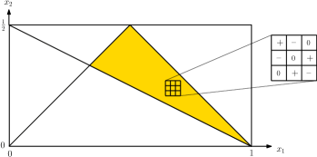
Figure 1. The domain $\Delta$ characterised by (4.2), and the square that defines the function $g$.

Holroyd’s example can be generalised to random partitions with infinitely many elements as follows. Let $a\in(\frac{3}{4},1]$. Choose $(X_{1},X_{2},X_{3})$ with the constraint $X_{1}+X_{2}+X_{3}=a$; then choose an arbitrary random partition on the remaining interval $[0,1-a]$. The domain (4.2) is replaced by $x_{1}\geq x_{2}\geq a-x_{1}-x_{2}\geq 1-a$ (it is nonempty for $a>\nicefrac{{3}}{{4}}$). The same argument then applies. It is also possible to take $a$ to be random.

5. Acknowledgements

We thank Christina Goldschmidt for discussions and for pointing out the examples from the Brownian bridge and pseudo-bridge, and the reference [15]; Jon Warren for further discussions about the pseudo-bridge; Jeff Steif and Johan Tykesson for discussions about their paper [20]; and Alexander Holroyd for explaining his example. We also thank the three referees for positive and helpful comments. We gratefully acknowlege support from the UoC Forum Classical and quantum dynamics of interacting particle systems. JEB gratefully acknowledges support from Vetenskapsrådet grant 2015-0519 and Ruth och Nils-Erik Stenbäcks stiftelse. CM is grateful to the EPSRC for support through the fellowship EP/R022186/1.

References

- [1]
- [2] M. Aizenman, B. Nachtergaele, Geometric aspects of quantum spin states, Comm. Math. Phys. 164, 17–63 (1994)
- [3] J. Bertoin, Random fragmentation and coagulation processes, Cambridge Studies Adv. Math. 102, Cambridge University Press (2006)
- [4] V. Betz, D. Ueltschi, Spatial random permutations and Poisson-Dirichlet law of cycle lengths, Electr. J. Probab. 16, 1173–1192 (2011)
- [5] P. Billingsley, Convergence of Probability Measures, 2nd ed, Wiley (1999)
- [6] J.E. Björnberg, J. Fröhlich, D. Ueltschi, Quantum spins and random loops on the complete graph, arXiv:1811.12834
- [7] J.E. Björnberg, M. Kotowski, B. Lees, P. Miłoś, The interchange process with reversals on the complete graph, Electr. J. Probab. 24, paper no. 108 (2019)
- [8] P. Diaconis, D. Freedman, Iterated random functions, SIAM review 41.1: 45-76, (1999)
- [9] W. J. Ewens, The sampling theory of selectively neutral alleles, Theor. Popul. Biol. 3, 87–112 (1972)
- [10] P. D. Feigin, and R. L. Tweedie. Linear functionals and Markov chains associated with Dirichlet processes, Math. Proc. Cambridge Phil. Soc. 105(3) (1989)
- [11] C. Goldschmidt, D. Ueltschi, and P. Windridge, Quantum Heisenberg models and their probabilistic representations, Entropy and the Quantum II, Contemp. Math. 552, 177–224 (2011)
- [12] J. F. C. Kingman, Random discrete distributions, J. Royal Statist. Soc. B 37, 1–22 (1975)
- [13] J. F. C. Kingman, The representation of partition structures, J. London Math. Soc. 2.2, 374–380 (1978)
- [14] Y. Peres, W. Schlag and B. Solomyak. Sixty years of Bernoulli convolutions, Fractal geometry and stochastics II, 39–65, Birkhäuser, Basel (2000)
- [15] J. Pitman, Random weighted averages, partition structures and generalized arcsine laws, arXiv/1804.07896 (2018)
- [16] J. Pitman, M. Yor, The two-parameter Poisson-Dirichlet distribution derived from a stable subordinator, Ann. Probab. 25, 855–900 (1997)
- [17] S. G. Samko, A. A. Kilbas and O. I. Marichev, Fractional integrals and derivatives: theory and applications, Gordon and Breach (1993)
- [18] O. Schramm, Compositions of random transpositions, Israel J. Math. 147, 221–243 (2005)
- [19] S. Sosnovskiy, On financial applications of the two-parameter Poisson-Dirichlet distribution, arXiv:1501.01954 (2015)
- [20] J. E. Steif and J. Tykesson, Generalized Divide and Color models, to appear in ALEA, arXiv:1702.04296
- [21] B. Tóth, Improved lower bound on the thermodynamic pressure of the spin Heisenberg ferromagnet, Lett. Math. Phys. 28, 75–84 (1993)
- [22] D. Ueltschi, Random loop representations for quantum spin systems, J. Math. Phys. 54, 083301, 1–40 (2013)