Time-resolved buildup of two-slit-type interference from a single atom

Abstract

A photoelectron forced to pass through two atomic energy levels before receding from the residual ion shows interference fringes in its angular distribution as manifestation of a two-slit-type interference experiment in wave-vector space. This scenario was experimentally realized by irradiating a Rubidium atom by two low-intensity continuous-wave lasers Pursehouse et al. (2019). In a one-photon process the first laser excites the 5p level while the second uncorrelated photon elevates the excited population to the continuum. This same continuum state can also be reached when the second laser excites the 6p state and the first photon then triggers the ionization. As the two lasers are weak and their relative phases uncorrelated, the coherence needed for generating the interference stems from the atom itself. Increasing the intensity or shortening the laser pulses enhances the probability that two photons from both lasers act at the same time, and hence the coherence properties of the applied lasers are expected to affect the interference fringes. Here, this aspect is investigated in detail, and it is shown how tuning the temporal shapes of the laser pulses allows for tracing the time-dependence of the interference fringes. We also study the influence of applying a third laser field with a random amplitude, resulting in a random fluctuation of one of the ionization amplitudes and discuss how the interference fringes are affected.

I Introduction

In a typical double-slit experiment interference fringes are formed on a screen placed behind the slits which are then traversed by particles of suitable wavelength. By blocking one of the slits, the spatial interference pattern disappears. In a recent wave-vector space double slit experiment Pursehouse et al. (2019) a photo-electron wave packet receding from a single atom is forced to pass through two energy levels within the atom, so that the levels play the role of the double-slit. As illustrated in Fig. 1, this is achieved by two low-intensity continuous-wave lasers which excite the $5p$ and $6p$ states of a Rubidium atom. The infrared light field can concurrently ionize the $6p$ state and the blue laser the $5p$ state. We image the interference in wave-vector space by scanning the photoelectron angular distribution. The interference pattern disappears if only one state is excited, demonstrating that the phase relationship between the interfering waves is imprinted by the atom. The two-lasers are not phase locked.

The $5p$ and $6p$ states thus represent "slits", which can be closed by detuning the respective laser fields, leading to non-resonant excitation and damped occupation of the specific intermediate state. This "damping" is however different from thermal damping, as it does not swiftly destroy the coherence. The interference in this case is affected because the two interfering amplitudes have largely different strengths.

In the experiment the interference term and the associated

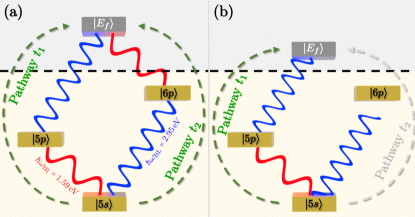
Figure 1: (a) Schematic representation of the atomic "double slit experiment" in Rubidium. The slits are represented by the bound and initially unoccupied $5p$ and $6p$ intermediate states which are resonantly excited by the infrared and blue laser pulses. The two lasers subsequently ionize the intermediate levels, giving rise to two ionization pathways $t_{1}$ and $t_{2}$. The photoelectron is transferred into the continuum with a finite kinetic energy $E_{f}$ without knowing which pathway was taken. (b) Closing one slit by detuning one of the two lasers which then inhibits the occupation of the respective intermediate state (in this example the $6p$ state). We hence obtain a conventional two-color photoionization process via a single ionization pathway. The energy level of the final state is now shifted down due to the detuning decreasing effectively $\varepsilon_{f}=\hbar\omega_{\rm BL}+\hbar\omega_{\rm IR}+\varepsilon_{5s}$.

difference in the phases of the amplitudes were recorded by essentially three measurements. First, both laser fields were set resonant to the $5p$ and $6p$ dipolar excitations leading to an ionization amplitude $t_{1}+t_{2}$ [cf. 1(a)]. In the second and third measurements, one of the two laser fields was detuned to close one of the ionization pathways [cf. 1(b)] to extract the individual amplitudes $t_{1}(t_{2})$. The ground state energy of the $5s$ Rb state is -4.177 eV while $E_{6p}=-1.589\,$eV and $E_{5p}=-2.950\,$eV. Thus, no other states in the bound spectrum of Rb are accessible by single-photon processes. An interesting point is that in the experiment the two cw (continuous wave) lasers (cf. Fig.1) were not phase locked and were weak. The calculations show that a random phase between these two lasers does not affect the interference. Thus the observed interference has to stem from the atom, while the photoelectron wave is propagating out to the detectors at infinity.

The question we are considering here is how the interference behaves when the number of photons (the laser intensity) increases, and hence one would expect an increase in the probability that a blue and red photon are absorbed at the same time. The same process applies when we consider much shorter pulses. In this case one would expect the phase relation between the laser pulses to be important, and it then becomes possible to access the time scale on which the interference pattern builds up and evolves. Unfortunately, due to experimental limitations we are currently not in a position to investigate these ideas in the laboratory, and therefore the current work is mostly theoretical.

In the final sections of this paper we discuss mechanisms for controlling and manipulating the interference phenomena between both ionization pathways. Atomic units are used throughout the paper.

II Propagation on a space-time grid

Within the single-particle picture the Rubidium atom is well described by the angular-dependent model potential introduced by Marinescu et al. Marinescu et al. (1994):

$$V_{\ell}(r)=-\frac{Z_{\ell}(r)}{r}-\frac{\alpha_{c}}{2r^{4}}\left[1-e^{-(r/r_{c})^{6}}\right],$$ (1)

where $\alpha_{c}$ is the static dipole polarizability of the positive-ion core and the effective radial charge $Z_{\ell}(r)$ is given by

$$Z_{\ell}(r)=1+(z-1)e^{-a_{1}r}-r(a_{3}+a_{4}r)e^{-a_{2}r},$$ (2)

with the nuclear charge $z$ and the cut-off parameter $r_{c}$ as well as the parameters $a_{1}-a_{4}$ fitted to experimental values. The optimized parameters are tabulated in Ref. Marinescu et al. (1994).

On a very fine space grid ($\Delta r=0.005$ a.u.) the radial wave functions of the atomic eigenstates ${\langle\boldsymbol{r}|\phi_{i}\rangle=R_{n_{i},\ell_{i}}(r)Y_{\ell_{i},m_{i}}(\Omega_{\boldsymbol{r}})}$ are found by (numerical) diagonalization of the matrix corresponding to the time-independent Hamiltonian $\hat{H}_{0}=-(1/2)\partial_{r}^{2}+{\ell(\ell+1)/(2r^{2})}+V_{\ell}(r)$. In the presence of solenoidal and moderately intense electromagnetic fields the light-matter interaction Hamiltonian is given by $\hat{H}_{\rm int}(t)=-\boldsymbol{A}(\boldsymbol{r},t)\cdot\hat{\boldsymbol{p}}$ where $\boldsymbol{A}(\boldsymbol{r},t)$ is the vector potential and $\hat{\boldsymbol{p}}$ is the momentum operator.

To account for all multi-photon and multipole effects, a numerical propagation of the ground state wave function in the external vector potential is necessary, e.g. by the matrix iteration scheme Nurhuda and Faisal (1999). Exploiting the spherical symmetry of the atomic system, the time-dependent wave function is decomposed in spherical harmonics, i.e. $\Psi(\boldsymbol{r},t)=\sum_{\ell,m}^{\ell_{\rm max}}b_{\ell,m}(r,t)Y_{\ell,m}(\Omega_{\boldsymbol{r}})$. We therefore have to propagate $(\ell_{\rm max}+1)^{2}$ channel functions $b_{\ell,m}(r,t)$ which are coupled through the corresponding (dipole) matrix elements $\langle\ell^{\prime}m^{\prime}|\boldsymbol{A}\cdot\hat{\boldsymbol{p}}|m\ell\rangle$. Initially, the ground state channel is fully occupied by the 5s Rubidium orbital, i.e. ${\Psi(\boldsymbol{r},t\rightarrow-\infty)=\langle\boldsymbol{r}|\phi_{5s}\rangle}$ meaning ${b_{0,0}(r,t-\infty)=R_{n_{i}=5,\ell_{i}=0}(r)}$. Introducing a time $T_{\rm obs}$ where the external electromagnetic field perturbation is off, the wave function $\Psi(\boldsymbol{r},t)$ is propagated to a time $t>T_{\rm obs}$ where the photoelectron wave packet is fully formed. The radial grid is extended to $10^{4}$ a.u. to avoid nonphysical reflections at the boundaries. Additionally, we implemented absorbing boundary conditions by using an imaginary potential. The resulting simulation shows that the electron density at the final grid point $r_{N}$ is then smaller than the numerical error at the considered propagation times.
To obtain the scattering properties of the liberated electron, we project $\Psi(\boldsymbol{r},T_{\rm obs})$ onto a set of continuum wave functions which are given by the partial wave decomposition:

$$\langle\boldsymbol{r}|\varphi_{\boldsymbol{k}}^{(-)}\rangle=\sum_{\ell,m}i^{\ell}R_{k\ell}(r)e^{-i\delta_{\ell}(k)}Y^{*}_{\ell,m}(\Omega_{\boldsymbol{k}})Y_{\ell,m}(\Omega_{\boldsymbol{r}}).$$ (3)

Here, the kinetic energy is defined by $E_{k}=k^{2}/2$, $\delta_{\ell}(k)$ are the scattering phases and $R_{k\ell}(r)$ are radial wave functions satisfying the stationary radial Schrödinger equation for positive energies in the same pseudopotential $V_{\ell}(r)$ which is used for obtaining the bound spectrum. The scattering phases $\delta_{\ell}(k)={\rm arg}[\Gamma(1+\ell-i/k)]+\eta_{\ell}(k)$ consist of the well-known Coulomb phases (first term) and phase $\eta_{\ell}(k)$ characterizing the atomic-specific short-ranged deviation from the Coulomb potential. The radial wave functions are normalized to $\langle R_{k\ell}|R_{k^{\prime}\ell}\rangle=\delta(E_{k}-E_{k^{\prime}})$. Finally, the projection coefficients are given by

$$\begin{split}a_{\ell,m}(k)=&\,e^{i(E_{k}T_{\rm obs}+\delta_{\ell}(k)-\ell\pi/2)}\\ &\times\int_{r>r_{a}}{\rm d}r\,b_{\ell,m}(r,T_{\rm obs})R_{k\ell}(r).\end{split}$$ (4)

Here, we introduce the core radius $r_{a}$ and ensure that the integration region is outside the residual ion. The photoionization probability (differential cross section, abbreviated as DCS in the following) is defined as

$$\begin{split}{\rm DCS}=\frac{{\rm d}\sigma}{{\rm d}\Omega_{\boldsymbol{k}}}(E_{k},\Omega_{\boldsymbol{k}})\propto&\sum_{\ell,\ell^{\prime}}\sum_{m,m^{\prime}}a^{*}_{\ell^{\prime},m^{\prime}}(k)a_{\ell,m}(k)\\ &\times Y^{*}_{\ell^{\prime},m^{\prime}}(\Omega_{\boldsymbol{k}})Y_{\ell,m}(\Omega_{\boldsymbol{k}}).\end{split}$$ (5)

while the total cross section is $\sigma(E_{k})\propto\sum_{\ell,m}\sigma_{\ell,m}(E_{k})$ with $\sigma_{\ell,m}(E_{k})=|a_{\ell,m}(k)|^{2}$. Note that this treatment gives explicit insight into the population of the individual angular channels and their contributions to the photoelectron wave packet.

In the following two-color ionization of Rubidium, the electric fields of both pulses are modeled according to

$$E_{p}(t)=\epsilon_{p}\mathcal{E}_{p}\Omega(t+\Delta_{p})\cos(\omega_{p}(t+\Delta_{p})+\phi_{p})$$ (6)

with $p={\rm IR,BL}$ standing for the infrared and blue laser pulses, respectively. The polarization vectors are $\epsilon_{p}$, the temporal envelope is given by $\Omega(t)=\cos^{2}(\pi t/T_{d}^{p})$ for $t\in[-T_{d}^{p}/2,T_{d}^{p}/2]$ with the pulse duration $T_{d}^{p}=2\pi n_{p}/\omega_{p}$ determined by the number of optical cycles $n_{p}$. Further we introduce a temporal difference $\Delta_{p}$ and a phase difference $\phi_{p}$ to account for both laser fields originating from different sources, and which are hence not phase-locked. Without loss of generality we set $\phi_{\rm IR}=0$ and $\Delta_{\rm IR}=0$. Both laser fields are assumed to be linearly polarized in the $z$-direction so that the azimuthal angular quantum number $m$ is conserved. The number of angular channels then reduces to $\ell_{\rm max}+1$ and in the following treatment we omit the subscript $m$ for brevity.

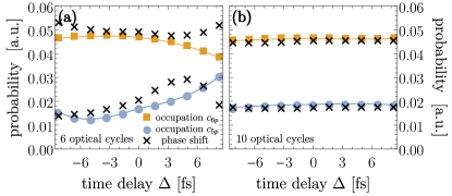
Figure 2: Occupation numbers of the $5p$ and $6p$ intermediate states after laser excitation, which depend on the time delay $\Delta$ and the phase difference between both pulses. (a) shows the results of the numerical propagation for six optical cycles. (b) corresponds to ten optical cycles. Dots indicate the results for $\phi=0$ radians and crosses belong to $\phi=2/3\pi$.

To balance the differences in the oscillator strengths between the $5s\rightarrow 5p$ and $5s\rightarrow 6p$ channels we used the field strengths $\mathcal{E}_{\rm BL}=0.05$ a.u. and $\mathcal{E}_{\rm IR}=0.007$ a.u. in the following simulations.

The aim here is to determine the influence of the phase differences on the resulting photoionization and occupation probabilities. In Fig. 2 we present the occupation numbers of the intermediate $5p$ and $6p$ states for two different laser configurations at a time $T_{\rm obs}$ after laser excitation, meaning both light pulses are completely extinguished and the photoelectron wave packet propagates freely in the Coulomb field of the residual Rubidium ion. Panel (a) corresponds to the case where both laser pulses have a length of six optical cycles. We see that both occupation numbers show a strong dependence on the temporal difference $\Delta$ as well as on a random phase difference $\phi$. The dots belong to $\phi=0$ while crosses indicate the results for a non-zero phase difference. Here, we show the occupation numbers for $\phi=2/3\pi$, which show a large difference to the case of $\phi=0$. In addition, we repeated the simulation for other numbers of the random phase difference and obtained similarly pronounced discrepancies. The situation changes completely when increasing the number of optical cycles as shown in panel (b). For ten optical cycles the influence of both the temporal and phase differences on the resulting occupation numbers is drastically reduced, pointing to the transition into the cw limit.

Already from the bounded properties we suspect the rather fast convergence of the photoionization process into a description within the frequency domain, which is characterized by infinitely long laser pulses characterised by delta distribution-like bandwidths. We can underline this observation by looking at the characteristics of the ejected photoelectron wave packet. In Fig. 3(a) we present the ionization probability of the angular channel $\ell=2$ characterized by the partial cross section $\sigma_{2}=\left|a_{\ell=2}(k)\right|^{2}$. As expected, the probability curve sharpens under an increase in the pulse lengths of both laser fields. While for $n_{p}=6$ a manifold of energy states in the continuum is excited, from $n_{p}=10$ upwards we see clearly the unfolding of a Gaussian-like peak around the final energy $E_{f}=E_{5s}+\hbar\omega_{\rm IR}+\hbar\omega_{\rm BL}$. In the case of 35 optical cycles the FHWM of the probability peak is around 0.07 eV.

It is also interesting to study the evolution of the quantum phase associated with the photoelectron wave packet, which can be expressed as $\varphi(k,\vartheta_{k})={\rm arg}\left[\sum_{\ell}a_{\ell}(k)Y_{\ell,0}(\Omega_{\boldsymbol{k}})\right]$. For 6 optical cycles, the angular channels with $\ell=0$ and $\ell=2$ already represent the dominant contributions to the photoelectron at the final energy around 0.4 eV, as expected for a two-color photoionization process of an initial $s$-state. The quantum phase is a result of interference between both partial waves and for the long pulse limit it may be mathematically expressed by Wätzel et al. (2014)

$$\varphi(k,\vartheta_{k})=\arctan\left[\frac{\sum_{\ell=0,2}S_{\ell}(k,\vartheta_{k})\sin(\phi_{\ell}(k))}{\sum_{\ell=0,2}S_{\ell}(k,\vartheta_{k})\cos(\phi_{\ell}(k))}\right]$$ (7)

with $S_{\ell}(k,\vartheta_{k})=\left|a_{\ell}(k)\right|Y_{\ell,0}(\Omega_{\boldsymbol{k}})$ and $\phi_{\ell}(k)={\rm arg}[a_{\ell}(k)]\simeq\delta_{\ell}(k)-\ell\pi/2$.

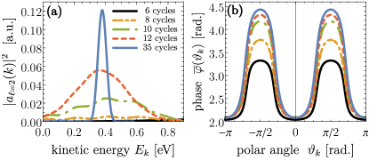
Figure 3: Properties of the ejected photoelectron. (a) Ionization probability of the angular channel $\ell=2$ for different pulse lengths of the incident IR and blue laser fields. (b) Angular variation of the averaged quantum phase $\overline{\varphi}(\vartheta_{k})$ in dependence on the number of optical cycles.

The quantum phase hence depends crucially on the scattering phases $\delta_{\ell}(k)$ and on the ratio between the transitions strengths into $\ell=2$ and $\ell=0$ angular channels respectively. We note that in principle $\varphi(k,\vartheta_{k})$ is an experimentally accessible quantity, since it can be recovered by integrating the Wigner time delay in photoionization defined as $\tau_{\rm W}(E_{k},\vartheta_{k})=({\rm d}/{\rm d}E_{k})\varphi(k,\vartheta_{k})$. This can be extracted from delay measurements that are possible due to recent experimental advances within the attosecond timeframe Schultze et al. (2010); Isinger et al. (2017). The measured atomic time delay $\tau_{\rm a}$ consists of an "intrinsic" contribution (Wigner time delay $\tau_{\rm W}$) upon the absorption of an XUV photon which can be interpreted as the group delay of the outgoing photoelectron wave packet due to the collision process. As mentioned above, it contains information about the internal quantum phase. The second term $\tau_{\rm cc}$ arises from continuum-continuum transitions due to the interaction of the laser probe field with the Coulomb potential and depends crucially on the experimental parameters. Hence, the difference $\tau_{\rm W}=\tau_{\rm a}-\tau_{\rm cc}$ provides access to the phase information $\varphi(k,\vartheta_{k})$.

In Fig.3(b) it is shown how the phase develops by increasing the pulse lengths (number of optical cycles). Here, we show the phase averaged over the ionization probability (total cross section $\sigma(E_{k})$): $\overline{\varphi}(\vartheta_{k})=\int{\rm d}E_{k}\,\sigma(E_{k})\varphi(k,\vartheta_{k})/\int{\rm d}E_{k}\,\sigma(E_{k})$. Interestingly for very short pulses ($n_{p}=6$) where the cross section is far from being centered around a final energy $E_{f}=E_{5s}+\hbar\omega_{\rm IR}+\hbar\omega_{\rm BL}$, the shape of the phase matches that extracted from simulations with longer pulses. As anticipated from earlier results, from ten cycles upwards the results converge quickly into the cw limit. As an example, this is seen since the discrepancy between the quantum phase for 12 and 35 optical cycles is smaller than 5%.

III From short pulses to the cw-limit

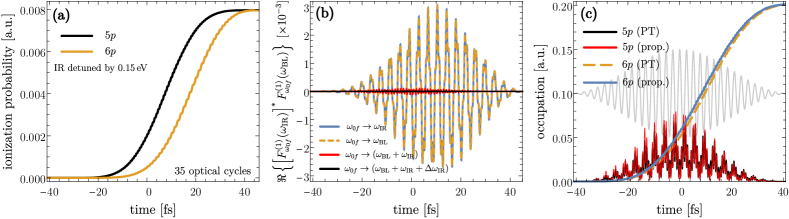
Figure 4: (a) Comparison between photoionization pathways via $5p$ and $6p$ intermediate states in the case of detuning $\delta\omega_{\rm IR}=0.15$ eV of the infrared field. The curves are extracted from Eq. (10). (b) Time dependence of the first-order product $\Re\{[F_{\omega_{0}}^{(1)}(t,-\omega_{\rm IR},0)]^{*}F_{\omega_{0}}^{(1)}(t,-\omega_{\rm BL},\Delta_{\rm BL})\}$ for different final energies. (c) Time dependent occupation numbers $c_{5p}(t)$ and $c_{6p}(t)$ extracted from perturbation theory and a full numerical treatment. The grey curve indicates the temporal variation of the IR laser field.

By considering the two-color ionization process using perturbation theory, we express the time-dependent wave function as $\Psi(\boldsymbol{r},t)=\sum_{\nu\ell}d_{\nu\ell}(t)e^{-{\rm i}E_{\nu\ell}t}\phi_{\nu\ell}(\boldsymbol{r})$. Note that the quantum number $\nu$ includes both the bound and the continuum states. The first order amplitude is given by:

$$\begin{split}d^{(1)}_{0\rightarrow f}(t)=&-\frac{1}{i}\sum_{\lambda=\pm 1}\left[\langle f|D_{\rm IR}|n\rangle\mathcal{E}_{\rm IR}F_{\omega_{0f}}^{(1)}(t,\lambda\omega_{\rm IR},\Delta=0)\right.\\ &\left.+e^{i\lambda\Delta\omega_{\rm BL}}\langle f|D_{\rm BL}|n\rangle\mathcal{E}_{\rm BL}F_{\omega_{0f}}^{(1)}(t,\lambda\omega_{\rm BL},\lambda\Delta)\right],\end{split}$$ (8)

where $D_{i}=\hat{\epsilon}_{i}\cdot\hat{d}$ ($i={\rm IR,BL}$) is the dipole operator, $\omega_{0f}=E_{f}-E_{0}$ and

$$F_{\omega_{0f}}^{(1)}(t,\omega,\Delta)=\int_{-\infty}^{t}\Omega(t^{\prime}+\Delta)e^{{\rm i}(\omega_{0f}+\omega)t^{\prime}}{\rm d}t^{\prime}.$$ (9)

Without loss of generality we assume both laser fields are described by the same temporal function $\Omega(t)=\cos^{2}[\pi t/T_{p}]$ so that both pulses have the same pulse length $T_{p}=2n_{p}\pi/\omega_{\rm IR}$. In the following discussion the number of optical cycles $n_{p}$ hence refers to the infrared laser field. For the squared-cosine shaped envelope $\Omega(t)$ of the pulses, the function $F_{\omega_{0}}^{(1)}(t,\omega,\Delta)$ can be obtained analytically and converges against $F_{\omega_{0}}^{(1)}(t,\omega,\Delta)\rightarrow\delta(\omega_{0}-\omega)$ for $T_{p}\rightarrow\infty$. The second order amplitude yields the following expression:

$$\begin{split}d^{(2)}_{0\rightarrow f}(t)=&-\sum_{i,j}\sum_{\lambda,\lambda^{\prime}=\pm 1}\sum_{n}e^{{\rm i}(\lambda\Delta_{j}\omega_{j}+\lambda^{\prime}\Delta_{i}\omega_{i})}\\ &\times\mathcal{E}_{j}\mathcal{E}_{i}\frac{\langle f|D_{j}|n\rangle\langle n|D_{i}|0\rangle}{\omega_{0n}-\omega_{i}}\\ &\times F^{(2)}_{\omega_{nf},\omega_{0n}}(t,\lambda\omega_{j},\lambda^{\prime}\omega_{i},\lambda\Delta_{j},\lambda^{\prime}\Delta_{i}),\end{split}$$ (10)

where again $i,j={\rm IR,BL}$. The second-order temporal function is defined as

$$\begin{split}F&{}^{(2)}_{\omega_{nf},\omega_{0n}}(t,\omega_{j},\omega_{i},\Delta_{j},\Delta_{i})=(\omega_{0n}-\omega_{i})\\ &\times\int_{-\infty}^{t}{\rm d}t^{\prime}\,\Omega(t^{\prime}+\Delta_{j})e^{{\rm i}(\omega_{nf}+\omega_{j})t^{\prime}}F^{(1)}_{\omega_{0n}}(t^{\prime},\omega_{i},\Delta_{i}).\end{split}$$ (11)

A closed expression for the second-order temporal function $F^{(2)}$ cannot be obtained analytically. However, a solution for $t>T_{p}/2$ (time of switch off) can be found and investigated for $T_{p}\rightarrow\infty$ (the continuous wave limit). It follows that in the many optical cycle limit we find energy conservation, i.e.

$$\lim_{n_{p}\rightarrow\infty}F^{(2)}_{\omega_{nf},\omega_{0n}}(t,-\omega_{j},-\omega_{i},\Delta_{j},\Delta_{i})=\frac{3\pi}{4}\delta(\omega_{0f}-\omega_{\rm j}-\omega_{\rm i})$$ (12)

Further, in this limit the individual temporal shifts $\Delta_{j}$ and $\Delta_{i}$ have no influence on the (second-order) transition amplitude. Thus, in the long (cw) pulse limit and for energies around $E_{f}=E_{0}+\hbar\omega_{0f}$, this behavior allows us to rewrite the resulting second-order transition amplitude:

$$\begin{split}d^{(2)}_{0\rightarrow f}\underset{n_{p}\rightarrow\infty}{\rightarrow}&\frac{3\pi}{4}\mathcal{E}_{\rm IR}\mathcal{E}_{\rm BL}e^{{\rm i}\Delta\omega_{\rm BL}}\sum_{n}\left[\frac{\langle f|D_{\rm IR}|n\rangle\langle n|D_{\rm BL}|0\rangle}{\omega_{n0}-\omega_{\rm BL}}\right.\\ &\left.+\frac{\langle f|D_{\rm BL}|n\rangle\langle n|D_{\rm IR}|0\rangle}{\omega_{n0}-\omega_{\rm IR}}\right],\end{split}$$ (13)

which is similar to the traditional form of the two-photon matrix element Toma and Muller (2002). From here we see directly that a random phase $\phi=\Delta\omega_{\rm BL}$ does not play any role (especially when analyzing the cross sections $\sim|d^{(2)}_{0\rightarrow f}|^{2}$.

Let us now come back to the two-color ionization process in the Rubidium atom. It is crucial for the first and second-order amplitudes to precisely evaluate the dipole matrix elements Amusia (2013)

$$\langle f|D_{i}|n\rangle=(-1)^{m_{f}+\ell_{>}}\begin{pmatrix}\ell_{f}&1&\ell_{n}\\ -m_{f}&0&m_{n}\end{pmatrix}\sqrt{\ell_{>}}\langle f||\hat{d}||n\rangle.$$ (14)

where $\ell_{>}={\rm max}(\ell_{f},\ell_{n})$ and the reduced radial matrix element $d_{\ell_{f}\ell_{n}}=\langle f||\hat{d}||n\rangle=\int_{0}^{\infty}{\rm d}r\,R_{f}(r)D_{i}R_{n}(r)$. One way to account, at least partially, for the the interaction between the valence and the core electrons Hameed et al. (1968) is to modify the operator $\hat{Q}_{L}$ as

$$\hat{Q}_{L}\rightarrow\hat{Q}_{L}\left[1-\frac{a_{c}^{(L)}}{r^{2L+1}}\left(1-e^{-(r/r_{c}^{\prime})^{2L+1}}\right)\right],$$ (15)

where $a_{c}^{(L)}$ is the $2^{L}$ tensor core polarizability and $r_{c}^{\prime}$ is an empirical cut-off radius (for Rb $r_{c}^{\prime}=4.339773$ a.u. Marinescu et al. (1994)). This physical picture behind the corrections is roughly that the valence electron with a dipole moment $\boldsymbol{d}$ induces (by virtue of its field) a (core) dipole moment $-\alpha_{c}\boldsymbol{d}/r^{3}$ (and higher multipoles). Then, the complete dipole moment becomes $\boldsymbol{d}(1-\alpha_{c}/r^{3})$. Note that in our case the Dipole operator $\hat{d}=\hat{Q}_{1}$. Using the modified dipole operator delivers very accurate matrix elements near the ionization threshold in comparison with experiments and more sophisticated theoretical models Petrov et al. (2000).

We learn from Eq. (13) that changing the electric field amplitudes $\mathcal{E}_{\rm IR}$ and $\mathcal{E}_{\rm BL}$ will not balance any differences between the matrix element products $\langle f|D_{\rm IR}|n\rangle\langle n|D_{\rm BL}|0\rangle$ and $\langle f|D_{\rm BL}|n\rangle\langle n|D_{\rm IR}|0\rangle$. Thus, to reach equipollent ionization pathways $E_{5s}\rightarrow E_{5p}\rightarrow E_{f}$ and $E_{5s}\rightarrow E_{6p}\rightarrow E_{f}$ we have to detune the laser frequency corresponding to the stronger bound-bound transition. Given the reduced matrix elements $\langle 5p||\hat{d}||5s\rangle=-5.158$ and $\langle 6p||\hat{d}||5s\rangle=0.468$, we have to detune the infrared field as shown in Fig 4(a). The curves are obtained from a numerical integration of Eq. (10). For $n=35$ optical cycles, a detuning of $\delta\omega_{\rm IR}=+0.15$ eV is required to allow the second-order transition amplitudes within each pathway to have the same magnitude. Note that the value of $\Delta\omega_{\rm IR}$ decreases by increasing the pulse lengths. In this vein we performed the simulation for 75 optical cycles and found that a detuning of only 0.07 eV is needed to reach equipollent ionization pathways (not shown for brevity).

Let us consider the time-dependent first order probability $P_{0\rightarrow f}^{(1)}(t)=\left|d^{(1)}_{0f}(t)\right|^{2}$ which reads explicitly

$$\begin{split}P_{0\rightarrow f}^{(0)}(t)=&\left|\langle f|D_{\rm IR}|n\rangle\mathcal{E}_{\rm IR}F_{\omega_{0f}}^{(1)}(t,-\omega_{\rm IR},0)\right|^{2}\\ &+\left|\langle f|D_{\rm BL}|n\rangle\mathcal{E}_{\rm BL}F^{(1)}_{\omega_{0f}}(t,-\omega_{\rm BL},\Delta_{\rm BL})\right|^{2}\\ &+2\mathcal{E}_{\rm IR}\mathcal{E}_{\rm BL}\langle f|D_{\rm IR}|n\rangle\langle f|D_{\rm BL}|n\rangle\\ &\times\Re\left\{F_{\omega_{0f}}^{(1)}(t,-\omega_{\rm IR})\left[F_{\omega_{0f}}^{(1)}(t,-\omega_{\rm BL},\Delta_{\rm BL})\right]^{*}\right\}.\end{split}$$ (16)

Here, we have to emphasize that all terms containing $+\omega_{i}$ are negligibly small which we refer to as the rotating wave approximation. The last term in the third line might look like a two-photon process but a closer inspection of the function $F_{\omega_{0}}^{(1)}(t,-\omega,\Delta)$ reveals that it sharply peaks around $\omega_{0}-\omega=0$ even for times close to $T_{p}/2$. Since $\omega_{f0}$ is fixed, the product between both $F^{(1)}$ functions is zero, so that

$$\begin{split}\lim_{T_{p}\rightarrow\infty}F_{\omega_{f0}}^{(1)}&(T_{p}/2,-\omega_{\rm IR},0)\left[F_{\omega_{f0}}^{(1)}(T_{p}/2,-\omega_{\rm BL},\Delta_{\rm BL})\right]^{*}\\ &=\delta(\omega_{f0}-\omega_{\rm BL})\delta(\omega_{f0}-\omega_{\rm BL}).\end{split}$$ (17)

As confirmation, in Fig. 4(b) we show the time-dependent product of the functions $F_{\omega_{0}}^{(1)}(t,-\omega_{\rm IR},0)$ and $F_{\omega_{0}}^{(1)}(t,-\omega_{\rm BL},\Delta_{\rm BL})$ for different $\omega_{f0}$. As stated above, all situations have in common that the product is zero at the time when the pulse is switched off, representing energy conservation. Finally, the first-order transitions for $t=T_{p}/2$ are given by

$$\begin{split}d^{(1)}_{0\rightarrow f}(t>T_{p}/2)=&-\frac{1}{2i}\left[\mathcal{E}_{\rm IR}\langle f|D_{\rm IR}|0\rangle\delta(w_{f0}-\omega_{\rm IR})\right.\\ &\left.+e^{{\rm i}\Delta\omega_{\rm BL}}\mathcal{E}_{\rm BL}\langle f|D_{\rm BL}|0\rangle\delta(w_{f0}-\omega_{\rm BL})\right].\end{split}$$ (18)

The energies of the blue and red photons are not sufficiently high to reach the continuum and only the two-photon matrix element developed in Eq. (10) gives insight into the properties of the photoelectron.

As a consequence, the amplitude $d^{(1)}$ describes the photoexcitation process of the intermediate $f=5p$ and $f=6p$ states. However, due to the sharp laser pulses the same final state $f$ cannot be excited by both photons. Hence, in the resulting photoexcitation probabilities $c_{f}=|d^{(1)}_{0\rightarrow f}(t>T_{p}/2)|^{2}$ the random phase $\phi=\Delta\omega_{\rm BL}$ does not play a role, which confirms the full-numerical results shown in Fig. 2(b).

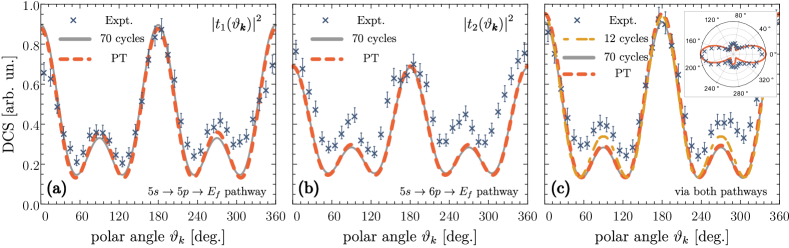
Figure 5: (a) Differential cross section (DCS) when the blue laser field is off-resonance, thereby effectively closing the second ionization pathway. Comparison between two theoretical models (PT:red and propagation:gray) and experimental results. For the propagation, the blue field was detuned by $\delta\omega_{\rm BL}=0.13$ eV. Further, the infrared field was slightly detuned by $\delta\omega_{\rm IR}=0.04$ eV to manipulate the ratio between both two-photon amplitudes (see discussions in Sec. III). (b) Same as in (a) with the infrared field completely off-resonance, effectively closing the first ionization pathway. The detuning amount is $\delta\omega_{\rm IR}=0.14$ eV. (c) Both laser fields resonant with associated pathways. To achieve pathway amplitudes that are comparable with experiment the infrared field was slightly detuned by $\delta\omega_{\rm IR}=0.04$ eV. The inset shows a polar plot of the DCS. All theoretical curves are scaled by the same factor and are shifted by a constant offset of 0.1 to aid comparison with the experimental data. The data points are reproduced from Ref.Pursehouse et al. (2019).

In panel 4(c) we present the occupation numbers $c_{5p}(t)=|\langle\phi_{5p}|\Psi(t)\rangle|^{2}$ and $c_{6p}(t)=|\langle\phi_{6p}|\Psi(t)\rangle|^{2}$ extracted from the perturbative treatment (PT) in Eq.(8) and the numerical simulation scheme developed in Sec. II. We find a remarkable agreement between the PT results and the full numerical treatment, demonstrating the transition into the cw limit and the validity of the perturbative treatment of the two-color ionization problem. Due to the detuning of the IR field the $c_{5s}(t)$ term decreases at the end of the pulse while the $c_{6p}(t)$ term belongs to resonant excitation ($5s\rightarrow 6p$) in the blue laser field. This is the reason for the nearly monotonous increase that is seen. We note that the corresponding Rabi frequencies $\Omega_{5s-5p}$ and $\Omega_{5s-6p}$ are very small which means the occupation numbers in Fig. 4(c) represent only the first segment of the first Rabi Cycle which can be identified by the characteristic quadratic dependence on the time.

IV Interference between both ionization pathways

As revealed by the two-photon matrix element in Eq. (13), both laser fields act simultaneously to produce the same final photoelectron state, and so we have to deal with two transition amplitudes $t_{1}$ and $t_{2}$ which are presented by the two terms. As already demonstrated in Sec. II the final state $|f\rangle$ is mainly described by a superposition of two angular channels $\ell=0$ and $\ell=2$. Thus, we may write

$$\begin{split}d^{(2)}_{0\rightarrow f}(\vartheta_{\boldsymbol{k}})&=t_{1}(\vartheta_{\boldsymbol{k}})+t_{2}(\vartheta_{\boldsymbol{k}})\\ &=\underbrace{S_{\ell=0}^{(t_{1})}(\vartheta_{\boldsymbol{k}})e^{i\phi_{\ell=0}(k_{f})}+S_{\ell=2}^{(t_{1})}(\vartheta_{\boldsymbol{k}})e^{i\phi_{\ell=2}(k_{f})}}_{t_{1}=|t_{1}|e^{i\varphi_{1}}}\\ &\quad+\underbrace{S_{\ell=0}^{(t_{2})}(\vartheta_{\boldsymbol{k}})e^{i\phi_{\ell=0}(k_{f})}+S_{\ell=2}^{(t_{2})}(\vartheta_{\boldsymbol{k}})e^{i\phi_{\ell=2}(k_{f})}}_{t_{2}=|t_{2}|e^{i\varphi_{2}}}.\end{split}$$ (19)

The final state is in the continuum and is defined by Eq. (3). Consequently, we can define

$$\begin{split}S^{(t_{i})}_{\ell_{f}}(\vartheta_{\boldsymbol{k}})=&(-1)^{2+\ell_{f}/2}\sqrt{1+\ell_{f}/2}\begin{pmatrix}\ell_{f}&1&1\\ 0&0&0\end{pmatrix}\begin{pmatrix}1&1&0\\ 0&0&0\end{pmatrix}\\ &\times\sum_{n}\frac{\langle E_{f}\ell_{f}||\hat{d}||n\rangle\langle n||\hat{d}||5s\rangle}{\omega_{0n}-\omega_{1}}\\ &\times\mathcal{E}_{\rm IR}\mathcal{E}_{\rm BL}F^{(2)}_{\omega_{nf},\omega_{0n}}(t\rightarrow\infty,-\omega_{2},-\omega_{1},0,0)\\ &\times Y_{\ell_{f},0}(\vartheta_{\boldsymbol{k}}).\end{split}$$ (20)

Here without loss of generality we set the time delays $\Delta_{\rm IR/BL}$ to zero since we are in the cw limit. For pathway $t_{1}$, $\omega_{1}=\omega_{\rm IR}$ and $\omega_{2}=\omega_{\rm BL}$, while for pathway $t_{2}$ the opposite is required. Further, $\phi_{\ell}(k)=\delta_{\ell}(k)-\ell\pi/2$ while the corresponding pathway phases $\varphi_{\rm i}$ are already defined in Eq. (7). Note, that $|t_{1}(\vartheta)|^{2}$ and $|t_{2}(\vartheta)|^{2}$ define the DCS for the individual pathways while the interference term between both pathways is given by

$$\begin{split}{\rm DCS}_{\rm interf.}&=t_{1}(\vartheta_{\boldsymbol{k}})t_{2}^{*}(\vartheta_{\boldsymbol{k}})+t_{2}(\vartheta_{\boldsymbol{k}})t_{1}^{*}(\vartheta_{\boldsymbol{k}})\\ &=\left|t_{1}(\vartheta_{\boldsymbol{k}})+t_{2}(\vartheta_{\boldsymbol{k}})\right|^{2}-(\left|t_{1}(\vartheta_{\boldsymbol{k}})\right|^{2}+\left|t_{2}(\vartheta_{\boldsymbol{k}})\right|^{2})\end{split}$$ (21)

The phase difference related to ${\rm DCS}_{\rm interf.}$ is given by

$$\begin{split}\Delta\varphi_{12}(\vartheta_{\boldsymbol{k}})=\cos^{-1}\left[\frac{t_{1}(\vartheta_{\boldsymbol{k}})t_{2}^{*}(\vartheta_{\boldsymbol{k}})+t_{2}(\vartheta_{\boldsymbol{k}})t_{1}^{*}(\vartheta_{\boldsymbol{k}})}{2\left|t_{1}(\vartheta_{\boldsymbol{k}})\right|\left|t_{2}(\vartheta_{\boldsymbol{k}})\right|}\right].\end{split}$$ (22)

The interference term is the result of differences in the ratios $S^{(t_{1})}_{\ell=2}/S^{(t_{1})}_{\ell=0}$ and $S^{(t_{2})}_{\ell=2}/S^{(t_{2})}_{\ell=0}$ between the $s$- and $d$- partial waves associated with the individual pathways $t_{1}$ and $t_{2}$. These ratios depend crucially on the reduced bound-continuum dipole matrix elements $\langle E_{f},\ell||\hat{d}||5p\rangle$ and $\langle E_{f},\ell||\hat{d}||6p\rangle$ as well as the bound-bound dipole matrix elements $\langle 5p||\hat{d}||5s\rangle$ and $\langle 6p||\hat{d}||5s\rangle$.

The perturbative treatment of the two-pathway ionization process shares some parallels with the theoretical description of the recently developed attosecond measurement techniques Dahlström et al. (2013). For instance, the occurrence and spectral characteristics of the $2q$th sideband in the RABBITT scheme Muller (2002) stem from the interference between two ionization pathways: the absorption of harmonic $H_{2q-1}$ or $H_{2q+1}$ plus absorption or emission of a laser photon with $\hbar\omega$. Hence, similarly to the effects studied in this work, the measured intensity of the side band depends on the phase difference between the quantum paths. In contrast to typical attosecond experiments, we create a bound wave packet upon absorption of the first photon. This case was studied in photoionization of Potassium where the spectral properties of the initially created bound wave packet was used to eliminate the influence of the dipole phase in the angle-integrated photoelectron spectrum making it possible to fully characterize the attosecond pulses Pabst and Dahlström (2016). Similar to the investigated experiment by Pursehouse and Murray, the underlying physical principle is the quantum interference of pathways corresponding to ionization from different energy levels. Moreover, a realistic many-body treatment revealed that correlation effects have only a minor influence in Alkali atoms which supports our theoretical treatment in this work.

In Fig. 5 we present the individual $t_{1}$ DCS (a), $t_{2}$ DCS (b) and the DCS corresponding to the coherent summation $t_{1}+t_{2}$ (c). In all panels we compare the ionization probabilities extracted from the full numerical and perturbative treatment with experimental results from measurements performed by Pursehouse and Murray Pursehouse et al. (2019). In the experiment the individual pathway cross sections are obtained by the appropriate detuning of the respective laser fields: To extract $|t_{1}|^{2}$ ($5s\rightarrow 5p\rightarrow E_{f}$) the blue laser beam is detuned to block occupation of the $6p$ state. To obtain the $|t_{2}|^{2}$ amplitude ($5s\rightarrow 6p\rightarrow E_{f}$), the infrared laser field is tuned to be off-resonant to the $5p$ transition. To obtain the total amplitude $|t_{1}+t_{2}|^{2}$ both laser pulses are on resonance to the respective $5s\rightarrow np$ transitions. As explained in Sec. III the infrared laser field is always slightly detuned by a fixed $\delta\omega_{\rm IR}$ so that both two-photon amplitudes $t_{1}$ and $t_{2}$ are of the same magnitude.

In panel 5(a) we show the DCS of the individual pathway 1. For the full numerical treatment with a number of 70 optical cycles we used a blue detuning of $\delta\omega_{\rm BL}=0.13$ eV while the red field detuning amounts to $\delta\omega_{\rm IR}=0.04$ eV. In the perturbative treatment ($n_{p}\rightarrow\infty$) we need a much smaller detuning (in the range of meV). Both theoretical models agree extraordinary well with the experiment in general, while minor discrepancies can be found around the maxima. A possible explanation is the shift of the final energy by nearly 0.17 eV in the full-numerical propagation (finite number of optical cycles) due to the detuning of both fields which changes slightly the ratios $S^{(t_{1})}_{\ell=2}/S^{(t_{1})}_{\ell=0}$. In comparison with the experiment, the theoretical models predict the correct shape of the DCS. They underestimate the data around $\vartheta_{\boldsymbol{k}}=90^{\circ}$ and $\vartheta_{\boldsymbol{k}}=270^{\circ}$, however agree well at $\vartheta_{\boldsymbol{k}}=0^{\circ}$ and $\vartheta_{\boldsymbol{k}}=180^{\circ}$ (along the polarization vectors). The same observations apply for the DCS of the second ionization pathway $|t_{2}|^{2}$ in panel 5(b). Figure 5(c) shows the photoionization probability $|t_{1}+t_{2}|^{2}$ when both laser fields are set to resonance with the respective $5s\rightarrow np$ transitions. Here, the infrared field is again detuned by a small $\delta\omega_{\rm IR}$ so that both amplitudes $t_{1}$ and $t_{2}$ have the same magnitude. In addition, we show here the result for rather short laser pulses with 12 optical cycles.

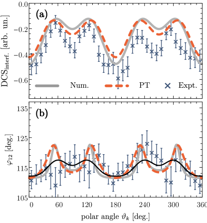
Figure 6: (a) Interference term ${\rm DCS}_{\rm interf.}$ for two theoretical models and experimental data. Parameters are the same as in Fig. 5. (b) Phase difference $\varphi_{12}$ between both ionization pathway amplitudes $t_{1}(\vartheta_{\boldsymbol{k}})$ and $t_{2}(\vartheta_{\boldsymbol{k}})$. The yellow line presents a fit of the experimental data to the symmetry-adapted function $f(\vartheta_{\boldsymbol{k}})=\sum_{n=0}^{2}a_{2n}\cos^{2n}(\vartheta_{\boldsymbol{k}})$. The data points are reproduced from Ref.Pursehouse et al. (2019).

Surprisingly, the DCS extracted from the short pulse calculations agree very well with the smaller maxima around $\vartheta_{\boldsymbol{k}}=90^{\circ}$ and $\vartheta_{\boldsymbol{k}}=270^{\circ}$. However, this rather accidental agreement must be considered within the experimental uncertainties.

In Fig. 6(a) we present the interference term ${\rm DCS}_{\rm interf.}$ for the two developed theoretical models and the experimental data. We see that the amplitude of the interference term is clearly non-zero and varies from $13\%$ to $55\%$ of the normalized signal shown in Fig. 5(c). In panel Fig. 6(b) we present the corresponding phase difference $\varphi_{12}(\vartheta_{\boldsymbol{k}})$ between the two-photon transition pathways $t_{1}$ and $t_{2}$. In comparison to all amplitudes, the agreement is less satisfactory which can be explained by the relatively large uncertainties due to error propagation through the arccos function Pursehouse et al. (2019). Interestingly the average value of the phase shift is accurately reproduced by both calculations. Under these conditions the predicted angular variation is not very pronounced and ranges from $110^{\circ}$ to $122^{\circ}$. Surprisingly, the models do not agree as well as for the DCS in Fig. 5, which points to the extreme sensitivity of the quantum phase to small changes in the transition matrix elements. The yellow curve represents a fit of the experimentally obtained phase difference to the symmetry-adapted function $\sum_{n=0}^{2}a_{2n}\cos^{2n}(\vartheta_{\boldsymbol{k}})$. It highlights the agreement with the theoretical prediction with respect to the general shape.

In the next section we will present mechanisms to manipulate, decrease and increase this modulation.

V Manipulation of the quantum interference

V.1 Role of the energy gap

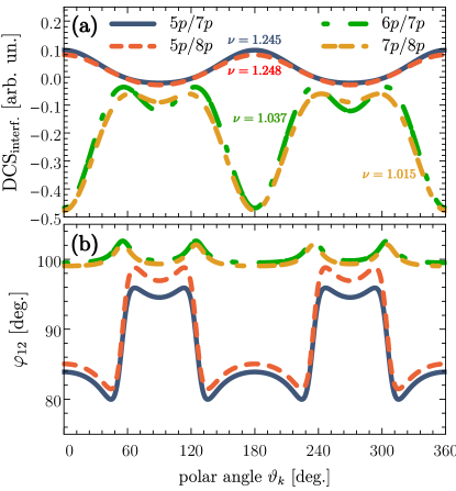
Figure 7: Interference cross section (a) and phase difference (b) $\varphi_{12}(\vartheta_{\boldsymbol{k}})$ for different intermediate state pairs extracted from the two-photon matrix element in Eq. (13). The IR field is detuned to reach equipollent pathway strengths. The numbers in panel (a) represent the ratio $\nu=(d^{(1)}_{2}/d^{(1)}_{0}):(d^{(2)}_{2}/d^{(2)}_{0})$.

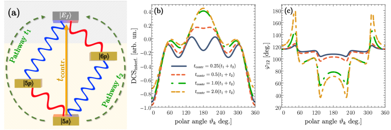
Figure 8: (a) Addition of a third laser pulse (orange) with amplitude $\mathcal{E}_{3}$ creates an additional third (direct) ionization pathway $t_{\rm contr}$ to the final energy $E_{f}$. The blue and IR pulses are the same as in Fig. 1. (b) Interference term ${\rm DCS}_{\rm interf}$ obtained from Eq. (23) for different strengths of the amplitude $t_{\rm contr}$ relative to $t_{1}+t_{2}$. (c) Angular dependence of the associated interference phase $\varphi_{12}$ between $t_{1}$ and $t_{2}$. All results are obtained by numerically calculation with pulse lengths of 75 optical cycles while the infrared and blue laser fields have the same field amplitudes and detunings as in the previous sections.

In Fig. 7 we present interference studies on different intermediate state pairs defining the two-color ionization amplitudes $t_{1}$ and $t_{2}$. The blue and the red curves present the interference between $5p/7p$ ($\Delta E=1.88$ eV) and $5p/8p$ ($\Delta E=2.13$ eV) states which have an increasing energy gap $\Delta E$ between them. The quantity $\nu=(d^{(t_{1})}_{\ell=2}/d^{(t_{1})}_{\ell=0})/(d^{(t_{2})}_{\ell=2}/d^{(t_{2})}_{\ell=0})$ represent the ratios of the bound-continuum reduced radial matrix elements between both pathways. As expected for higher Rydberg states this ratio converges quickly to the same number, i.e. the coupling of the $7p$ and $8p$ state to the continuum is similar. The interference for both state pairs is hence comparable. Note that the final energy $E_{f}=E_{5s}+\hbar\omega_{1}+\hbar\omega_{2}$ is larger in comparison to the $5p/6p$ case (0.84 eV and 1.09 eV). Interestingly, ${\rm DCS}_{\rm interf.}$ has a different shape and changes its sign in both cases, which has an impact on the angular modulation of the phase difference $\varphi_{12}$. Surprisingly while the amplitude is smaller in comparison with the $5p/6p$ case shown in Fig. 6, the angular variation of the phase is significantly more pronounced, ranging from $80^{\circ}$ to $100^{\circ}$. This highlights the change of sign of the interference term (negative sign of the argument of the arccos function means a phase larger than $90^{\circ}$).

The green and orange curves represent cases when we decrease the energy gap. We chose the intermediate state pairs $6p/7p$ ($\Delta E=0.51$ eV, $E_{f}=2.22$ eV) and $7p/8p$ ($\Delta E=0.25$ eV, $E_{f}=2.97$ eV). Intriguingly, the interference cross section remain unaffected when changing to higher lying state pairs. The amplitudes of ${\rm DCS}_{\rm interf.}$ ranges in both cases from 5% to 50% and is negative. However, the angular modulation of the phase difference $\varphi_{12}$ decreases drastically. We address this development with the dipole matrix element ratio $\nu$ which converges rapidly to 1, meaning the ratio between the $\ell=0$ and $\ell=2$ angular channels is nearly the same for both ionization pathways $t_{1}$ and $t_{2}$. According to Eq. (7) the individual phase shapes are then comparable.

From these results we learn that the angular modulation of the phase difference depends critically on the quantity $\nu$, while the overall amplitude of the interference term (${\rm DCS}_{\rm interf.}$) is more robust and reveals a dependence on the energy gap between the intermediate state pair defining $t_{1}$ and $t_{2}$.

V.2 laser-driven perturbation of ionization pathways

Another method for dynamic control of the interference phenomena is the addition of a third control pulse. As represented in the scheme in Fig. 8(a) the corresponding parameters are chosen in a way that initiates a weak one-photon process directly into the continuum, so that $\hbar\omega_{\rm contr.}=(E_{f}-E_{5s})/\hbar$. The field amplitude $\mathcal{E}_{\rm contr}$ is hence chosen in a way that the corresponding transition amplitude $t_{\rm contr}$ is of the same magnitude as that of the two-color pathways $t_{1}$ and $t_{2}$. As indicated in the modified scheme in Fig. 8(a), in the presence of all fields the total amplitude is given by the coherent sum $t_{\rm all}=t_{1}+t_{2}+t_{\rm contr.}$. To access the desired interference term ${\rm DCS}_{\rm interf}=t_{1}t_{2}^{*}+t_{1}^{*}t_{2}$ one has to then perform four different measurements: (i) with all fields on resonance to the intermediate and final states respectively, (ii) with the blue field to the $6p$ state off-resonance, (iii) with the red field to the $5p$ state off-resonance, and (iv) with both red and blue fields off-resonant (thereby blocking both pathways $t_{1}$ and $t_{2}$). The interference term is then given by

$${\rm DCS}_{\rm interf}=|t_{\rm all}|^{2}-(|t_{\rm(ii)}|^{2}+|t_{\rm(iii)}|^{2}-|t_{\rm(iv)}|^{2})$$ (23)

with $t_{\rm(ii)}=t_{1}+t_{\rm contr}$, $t_{\rm(iii)}=t_{2}+t_{\rm contr}$ and $t_{\rm(iv)}=t_{\rm contr}$.

In Fig. 8(b) we present the interference term for different strengths of the perturbation by the third (control) laser field. As expected, the additional one-photon ionization route has a large impact on the quantum interference between $t_{1}$ and $t_{2}$. Here, the field amplitude $\mathcal{E}_{\rm contr}$ has to be very low so that the associated $t_{\rm contr}$ is of the same magnitude as the two-photon pathways $t_{1}$ and $t_{2}$. In comparison to the unperturbed case shown in Fig.6(a), the magnitude of the interference is increased in the presence of the control field. In strong contrast to the previous findings, even the sign of the ${\rm DCS}_{\rm interf}$ can be changed by the effect of the additional one-photon process when the field amplitude is sufficiently large. It is therefore not surprising that the large impact seen here is directly transferred to the phase $\varphi_{12}$ associated with the quantum interference. As shown in Fig. 8(c), the angular variation is drastically increased due to the action of the controlling field. In the original experiment and theoretical treatment the modulation in the polar angle was smaller than 20^∘. Now we obtain strongly pronounced phase peaks and a rather complex angular structure of $\varphi_{12}$ with a variation covering more than 140^∘.

The addition of the third laser field helps to emphasize that the interference effect is not robust to statistical fluctuations, but is unique for every set of laser parameters. For this purpose we slightly detuned the blue laser field so that the $6p$ state was not excited [cf. Fig 9(a)]. The resulting interference phenomenon in the ionization channel then stems from the superposition of the two-photon pathway 1 (via $5p$ photoexcitation) and the one-photon direct photoionization amplitude mediated by $E_{\rm contr.}$. By tuning the parameters of the third field so that the transition strength of the amplitude $t_{\rm contr.}$ is equal to $t_{1}$ we obtain a characteristic interference as shown by the dark blue curve in Fig. 9(b). We then varied the amplitude of the control field in a way that $t_{\rm contr.}\in[-1.0t_{1},1.0t_{1}]$ by use of a random number generator. The additional curves in the figure show a statistical average based on the total number of random amplitudes input to the model. One can clearly see a trend that increasing the number of random events decreases the interference effect. This shows that for an infinite number of measurements the resulting interference would disappear.

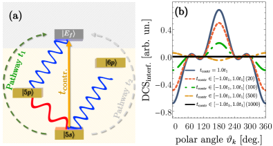
Figure 9: Stochastic nature of the interference effect. In this example one of the ionization pathways is closed by slight detuning of the laser field. We hence find interference between the two-photon amplitude (pathway 1) and the one-photon transition initiated by the third control field $E_{3}(t)$ (scheme panel a). (b) The stochastic nature of the interference effect: the amplitude of the one-photon process is randomly varied between $-1.0t_{1}$ and $+1.0t_{1}$. The curves show the dependence on the number of random amplitudes with the reference to $t_{\rm contr.}=1.0t_{1}$ (blue line). Numbers in the round brackets denote the number of amplitudes used for the statistical average (see text for details).

VI Conclusions

In this paper we have presented a theoretical investigation of experimental interference studies in a single Rubidium atom. We have systematically demonstrated the transition from the short-pulse into the continuous wave regime, and the evolution of the occupation numbers, photoionization probability and quantum phase under an increase of the pulse lengths. We find that for pulse lengths of more than ten optical cycles the theoretical description of the ionization scheme via the two-photon matrix element in the frequency regime is sufficient, and that this provides all the physical information required for interference studies.

Our theoretical model provides generally good agreement with the experimental data and predicts a pronounced interference amplitude ${\rm DCS}_{\rm interf.}$ while the angular variation of the associated phase difference $\varphi_{12}$ is relatively weak. In this treatment we have developed various strategies to manipulate the quantum interference between both photoionization pathways $t_{1}$ and $t_{2}$. As an example, we can change the populations of the intermediate states by laser detuning which introduces an imbalance between both pathways so as to change the interference phenomena. Further, by choosing different state pairs $n_{1}p$ and $n_{2}p$ we change the energy difference and coupling to the continuum, which again markedly changes the quantum interference. A new method which does not change the intermediate state pairs and the parameters of the blue and infrared laser fields is the addition of a third control laser field which perturbs the original transition pathways $t_{1}$ and $t_{2}$. An appropriate tuning of the corresponding one-photon transition amplitude into the continuum can even invert the sign of the interference amplitude, as well as produce a much more pronounced angular variation of the interference phase. There is no analogy to this third control in the conventional double slit experiments.

As well as the addition of a third pulse, there are several other possibilities to explore the behaviour of the interference phenomenon. As an example, one can show that in Alkali atoms quadrupole transitions into the continuum reveal Cooper minima at kinetic energies below 1eV. Thus, one can choose intermediate state pairs which lead to final energies in the region of such Cooper minima while such quadrupole transitions at low intensity are generally accessible by structured light fields Schmiegelow et al. (2016). Further work will hence be dedicated to studying these two-pathway interference effects with inhomogeneous light-induced quadrupole transitions.

References

- Pursehouse et al. (2019) J. Pursehouse, A. J. Murray, J. Wätzel, and J. Berakdar, Phys. Rev. Lett. 122, 053204 (2019).
- Marinescu et al. (1994) M. Marinescu, H. Sadeghpour, and A. Dalgarno, Phys. Rev. A 49, 982 (1994).
- Nurhuda and Faisal (1999) M. Nurhuda and F. H. Faisal, Phys. Rev. A 60, 3125 (1999).
- Wätzel et al. (2014) J. Wätzel, A. Moskalenko, Y. Pavlyukh, and J. Berakdar, J. Phys. B: At. Mol. Opt. Phys. 48, 025602 (2014).
- Schultze et al. (2010) M. Schultze, M. Fieß, N. Karpowicz, J. Gagnon, M. Korbman, M. Hofstetter, S. Neppl, A. L. Cavalieri, Y. Komninos, T. Mercouris, et al., Science 328, 1658 (2010).
- Isinger et al. (2017) M. Isinger, R. Squibb, D. Busto, S. Zhong, A. Harth, D. Kroon, S. Nandi, C. Arnold, M. Miranda, J. M. Dahlström, et al., Science 358, 893 (2017).
- Toma and Muller (2002) E. Toma and H. Muller, J. Phys. B: At. Mol. Opt. Phys. 35, 3435 (2002).
- Amusia (2013) M. Y. Amusia, Atomic photoeffect (Springer Science & Business Media, 2013).
- Hameed et al. (1968) S. Hameed, A. Herzenberg, and M. James, J. Phys. B: At. Mol. Phys. 1, 822 (1968).
- Petrov et al. (2000) I. Petrov, V. Sukhorukov, E. Leber, and H. Hotop, Eur. Phys. J. D 10, 53 (2000).
- Dahlström et al. (2013) J. M. Dahlström, D. Guénot, K. Klünder, M. Gisselbrecht, J. Mauritsson, A. L’Huillier, A. Maquet, and R. Taïeb, Chem. Phys. 414, 53 (2013).
- Muller (2002) H. . G. Muller, Appl. Phys. B 74, s17 (2002).
- Pabst and Dahlström (2016) S. Pabst and J. M. Dahlström, Phys. Rev. A 94, 013411 (2016).
- Schmiegelow et al. (2016) C. T. Schmiegelow, J. Schulz, H. Kaufmann, T. Ruster, U. G. Poschinger, and F. Schmidt-Kaler, Nat. Commun. 7, 12998 (2016).