Dynamically orthogonal tensor methods for high-dimensional nonlinear PDEs

Alec Dektor Daniele Venturi Department of Applied Mathematics
University of California Santa Cruz
Santa Cruz, CA 95064
venturi@ucsc.edu
Abstract

We develop new dynamically orthogonal tensor methods to approximate multivariate functions and the solution of high-dimensional time-dependent nonlinear partial differential equations (PDEs). The key idea relies on a hierarchical decomposition of the approximation space obtained by splitting the independent variables of the problem into disjoint subsets. This process, which can be conveniently be visualized in terms of binary trees, yields series expansions analogous to the classical Tensor-Train and Hierarchical Tucker tensor formats. By enforcing dynamic orthogonality conditions at each level of binary tree, we obtain coupled evolution equations for the modes spanning each subspace within the hierarchical decomposition. This allows us to effectively compute the solution to high-dimensional time-dependent nonlinear PDEs on tensor manifolds of constant rank, with no need for rank reduction methods. We also propose new algorithms for dynamic addition and removal of modes within each subspace. Numerical examples are presented and discussed for high-dimensional hyperbolic and parabolic PDEs in bounded domains.

journal: arXiv

1 Introduction

High-dimensional partial differential equations (PDEs) arise in many areas of engineering, physical sciences and mathematics. Classical examples are equations involving probability density functions (PDFs) such as the Fokker-Plank equation [55], the Liouville equation [64, 18], or the Boltzmann equation [12, 44]. Other types of high-dimensional PDEs can be obtained as finite-dimensional approximations of functional differential equations [63], such as the Hopf equation of turbulence [30, 31, 46], the Schwinger-Dyson equation of quantum mechanics [32], or the Martin-Siggia-Rose formulation of classical statistical dynamics [45, 33, 34, 50]. Computing the solution to high-dimensional PDEs is a challenging problem that requires approximating high-dimensional functions, i.e., the solution to the PDE, and then developing appropriate numerical schemes to compute such functions accurately. Classical numerical methods based on tensor product representations are not viable in high-dimensions, as the number of degrees of freedom grows exponentially fast with the dimension. To address this problem there have been substantial research efforts in recent years on high-dimensional numerical approximation theory. Techniques such as sparse collocation [10, 17, 7, 23, 47], high-dimensional model representations (HDMR) [42, 11, 6] and, more recently, deep neural networks [51, 52, 66] and tensor methods [37, 5, 9, 28, 16, 39] were proposed to mitigate the exponential growth of the degrees of freedom, the computational cost and memory requirements.

In this paper, we develop a new dynamically orthogonal tensor method to approximate multivariate functions and the solution of high-dimensional time-dependent nonlinear PDEs. The key idea relies on a hierarchical decomposition of the function space in terms of a sequence of nested subspaces of smaller dimension. Such decomposition is induced by by splitting the independent variables of the problem recursively into two disjoint subsets which can conveniently be visualized by binary trees. In particular, we study two classes of trees which are analogous to the Tensor-Train (TT) [48] and Hierarchical Tucker (HT) [26] tensor formats. By enforcing dynamic orthogonality (DO) [57] or bi-orthogonality (BO) [13] conditions at each level of the TT or the HT binary tree, we obtain coupled evolution equations for the modes spanning each subspace within the hierarchy. This allows us to represent the time evolution of high-dimensional functions and compute the solution of high-dimensional time-dependent nonlinear PDEs on a tensor manifold with constant rank. This formulation has several advantages over classical numerical tensor methods. In particular, the hard-to-compute nonlinear projection [43, 38] that maps the solution of high-dimensional PDEs onto a tensor manifold with constant rank [60] here is represented explicitly by the hierarchical DO/BO propagator111The hierarchical DO/BO propagator is nonlinear even for linear PDEs. Such nonlinearity implicitly represnts the projection onto a tensor manifold with constant rank., i.e., by a system of coupled one-dimensional nonlinear PDEs. In other words, there is no need to perform tensor rank reduction [24, 26, 40], rank-constrained temporal integration [43, 38], or Riemannian optimization [59], when solving high-dimensional PDEs with the hierarchical subspace decomposition method we propose222Classical numerical tensor methods for high-dimensional PDEs with explicit time stepping schemes require rank-reduction to project the solution back into the tensor manifold with prescribed rank (see [63] §5.5), the so-called retraction step [59]. This can be achieved, e.g., by a sequence of suitable matricizations followed by hierarchical singular value decomposition [24, 26, 40], or by optimization [59, 39, 9, 20, 56, 35]. Rank reduction can be computationally intensive, especially if performed at each time step. Tensor methods with implicit time stepping suffer from similar issues. In particular, the nonlinear system that yields the solution at the next time step needs to be solved on a tensor manifold with constant rank by using, e.g., Riemannian optimization algorithms [59, 60, 22]..

This paper is organized as follows. In Section 2 we introduce a recursive bi-orthogonal decomposition method for time-independent multivariate functions, develop error estimates and provide simple examples of application. In Section 3 we extend the recursive bi-orthogonal decomposition to time-dependent functions, and develop a hierarchy of nested time-dependent orthogonal projections generalizing the DO and BO conditions to tensor formats with multiple levels. We also prove that the approximations resulting from the BO and the DO conditions are equivalent, in the sense that they span the same function spaces. In Section 4, we apply the recursive subspace decomposition method to compute the solution of high-dimensional nonlinear PDEs. In Section 5 we provide numerical examples demonstrating the accuracy and computational effectiveness of the recursive subspace decomposition method we propose. Specifically we study high-dimensional hyperbolic and parabolic PDEs. The main findings are summarized in Section 6.

2 Recursive bi-orthogonal decomposition of time-independent multivariate functions

Let ΩΩ\Omega be a subset of dsuperscript𝑑\mathbb{R}^{d} (d2𝑑2d\geq 2) that contains an open set333If ΩdΩsuperscript𝑑\Omega\subseteq\mathbb{R}^{d} contains an open set then dim(Ω)=ddimΩ𝑑\text{dim}(\Omega)=d., and let

u:Ω:𝑢Ωu:\Omega\to\mathbb{R} (1)

be a multivariate function which we assume to be an element of a separable Hilbert space (Ω)Ω\mathcal{H}(\Omega). A possible choice of such Hilbert space is the Sobolev space

Hk(Ω)={uL2(Ω):D𝜶uL2(Ω)for all|𝜶|k},k=0,1,2,formulae-sequencesuperscript𝐻𝑘Ωconditional-set𝑢superscript𝐿2Ωformulae-sequencesuperscript𝐷𝜶𝑢superscript𝐿2Ωfor all𝜶𝑘𝑘012H^{k}(\Omega)=\left\{u\in L^{2}(\Omega)\,:\,D^{\bm{\alpha}}u\in L^{2}(\Omega)\quad\text{for all}\quad|\bm{\alpha}|\leq k\right\}\ ,\qquad k=0,1,2,\dots (2)

where 𝜶=(α1,,αd)𝜶subscript𝛼1subscript𝛼𝑑\bm{\alpha}=(\alpha_{1},\dots,\alpha_{d}) is a multi-index and

D𝜶u=|𝜶|ux1α1xdαd,|𝜶|=α1++αd.formulae-sequencesuperscript𝐷𝜶𝑢superscript𝜶𝑢superscriptsubscript𝑥1subscript𝛼1superscriptsubscript𝑥𝑑subscript𝛼𝑑𝜶subscript𝛼1subscript𝛼𝑑D^{\bm{\alpha}}u=\frac{\partial^{|\bm{\alpha}|}u}{\partial x_{1}^{\alpha_{1}}\dots\partial x_{d}^{\alpha_{d}}},\qquad|\bm{\alpha}|=\alpha_{1}+\dots+\alpha_{d}. (3)

Note that (2) includes the classical Lebesgue space L2(Ω)=H0(Ω)superscript𝐿2Ωsuperscript𝐻0ΩL^{2}(\Omega)=H^{0}(\Omega). We equip (2) with the standard inner product

f,gHk(Ω)=|𝜶|kΩD𝜶f(𝒙)D𝜶g(𝒙)𝑑x1𝑑xd.subscript𝑓𝑔superscript𝐻𝑘Ωsubscript𝜶𝑘subscriptΩsuperscript𝐷𝜶𝑓𝒙superscript𝐷𝜶𝑔𝒙differential-dsubscript𝑥1differential-dsubscript𝑥𝑑\langle f,g\rangle_{H^{k}(\Omega)}=\sum_{|\bm{\alpha}|\leq k}\int_{\Omega}D^{\bm{\alpha}}f(\bm{x})D^{\bm{\alpha}}g(\bm{x})dx_{1}\dots dx_{d}. (4)

If needed, this inner product can be weighted by a non-negative separable density ρ1(x1)ρd(xd)subscript𝜌1subscript𝑥1subscript𝜌𝑑subscript𝑥𝑑\rho_{1}(x_{1})\cdots\rho_{d}(x_{d}). Any separable Hilbert space is isomorphic to L2superscript𝐿2L^{2}, and it can be represented as a tensor product of two Hilbert spaces [53, p.51], i.e.,

12.tensor-productsubscript1subscript2\mathcal{H}\cong\mathcal{H}_{1}\otimes\mathcal{H}_{2}. (5)

The spaces 1subscript1\mathcal{H}_{1} and 2subscript2\mathcal{H}_{2} may be specified by partitioning the spatial variables {x1,,xd}subscript𝑥1subscript𝑥𝑑\{x_{1},\ldots,x_{d}\} into two disjoint subsets. This is equivalent to represent the domain ΩΩ\Omega as a Cartesian product of two sub-domains (whenever possible). For instance, consider the partition

Ω=Ω(1,,p)×Ω(p+1,,d)ΩsuperscriptΩ1𝑝superscriptΩ𝑝1𝑑\Omega=\Omega^{(1,\ldots,p)}\times\Omega^{(p+1,\ldots,d)} (6)

induced by the following splitting of the spatial variables

(x1,x2,,xd)inΩ=((x1,,xp)inΩ(1,,p),(xp+1,,xd)inΩ(p+1,,d)).subscriptsubscript𝑥1subscript𝑥2subscript𝑥𝑑inΩsubscriptsubscript𝑥1subscript𝑥𝑝insuperscriptΩ1𝑝subscriptsubscript𝑥𝑝1subscript𝑥𝑑insuperscriptΩ𝑝1𝑑\underbrace{(x_{1},x_{2},\ldots,x_{d})}_{\text{in}\,\,\Omega}=(\underbrace{(x_{1},\ldots,x_{p})}_{\text{in}\,\,\Omega^{(1,\ldots,p)}},\underbrace{(x_{p+1},\ldots,x_{d})}_{\text{in}\,\,\Omega^{(p+1,\ldots,d)}}). (7)

In this setting, the Sobolev space (2) admits the following decomposition

Hk(Ω)Hk(Ω(1,,p))Hk(Ω(p+1,,d)).superscript𝐻𝑘Ωtensor-productsuperscript𝐻𝑘superscriptΩ1𝑝superscript𝐻𝑘superscriptΩ𝑝1𝑑H^{k}(\Omega)\cong H^{k}\left(\Omega^{(1,\ldots,p)}\right)\otimes H^{k}\left(\Omega^{(p+1,\ldots,d)}\right). (8)

The inner products within each subspace Hk(Ω(1,,p))superscript𝐻𝑘superscriptΩ1𝑝H^{k}\left(\Omega^{(1,\ldots,p)}\right) and Hk(Ω(p+1,,d))superscript𝐻𝑘superscriptΩ𝑝1𝑑H^{k}\left(\Omega^{(p+1,\ldots,d)}\right) can be defined, respectively, as

f,gHk(Ω(1,,p))=α1++αpkΩ(1,,p)α1++αpfx1α1xpαpα1++αpgx1α1xpαp𝑑x1𝑑xp,subscript𝑓𝑔superscript𝐻𝑘superscriptΩ1𝑝subscriptsubscript𝛼1subscript𝛼𝑝𝑘subscriptsuperscriptΩ1𝑝superscriptsubscript𝛼1subscript𝛼𝑝𝑓superscriptsubscript𝑥1subscript𝛼1superscriptsubscript𝑥𝑝subscript𝛼𝑝superscriptsubscript𝛼1subscript𝛼𝑝𝑔superscriptsubscript𝑥1subscript𝛼1superscriptsubscript𝑥𝑝subscript𝛼𝑝differential-dsubscript𝑥1differential-dsubscript𝑥𝑝\langle f,g\rangle_{H^{k}\left(\Omega^{(1,\ldots,p)}\right)}=\sum_{\alpha_{1}+\dots+\alpha_{p}\leq k}\int_{\Omega^{(1,\ldots,p)}}\frac{\partial^{\alpha_{1}+\dots+\alpha_{p}}f}{\partial x_{1}^{\alpha_{1}}\dots\partial x_{p}^{\alpha_{p}}}\frac{\partial^{\alpha_{1}+\dots+\alpha_{p}}g}{\partial x_{1}^{\alpha_{1}}\dots\partial x_{p}^{\alpha_{p}}}dx_{1}\cdots dx_{p}, (9)

and

f,gHk(Ω(p+1,,d))=αp+1++αdkΩ(p+1,,d)αp+1++αdfxp+1αp+1xdαdαp+1++αdgxp+1αp+1xdαd𝑑xp+1𝑑xd.subscript𝑓𝑔superscript𝐻𝑘superscriptΩ𝑝1𝑑subscriptsubscript𝛼𝑝1subscript𝛼𝑑𝑘subscriptsuperscriptΩ𝑝1𝑑superscriptsubscript𝛼𝑝1subscript𝛼𝑑𝑓superscriptsubscript𝑥𝑝1subscript𝛼𝑝1superscriptsubscript𝑥𝑑subscript𝛼𝑑superscriptsubscript𝛼𝑝1subscript𝛼𝑑𝑔superscriptsubscript𝑥𝑝1subscript𝛼𝑝1superscriptsubscript𝑥𝑑subscript𝛼𝑑differential-dsubscript𝑥𝑝1differential-dsubscript𝑥𝑑\langle f,g\rangle_{H^{k}\left(\Omega^{(p+1,\ldots,d)}\right)}=\sum_{\alpha_{p+1}+\dots+\alpha_{d}\leq k}\int_{\Omega^{(p+1,\ldots,d)}}\frac{\partial^{\alpha_{p+1}+\dots+\alpha_{d}}f}{\partial x_{p+1}^{\alpha_{p+1}}\dots\partial x_{d}^{\alpha_{d}}}\frac{\partial^{\alpha_{p+1}+\dots+\alpha_{d}}g}{\partial x_{p+1}^{\alpha_{p+1}}\dots\partial x_{d}^{\alpha_{d}}}dx_{p+1}\cdots dx_{d}. (10)

A representation of the multivariate function (1) in the tensor product space (8) has the general form

u(x1,,xd)=i,j=1aijφi(1,,p)(x1,,xp)φj(p+1,,d)(xp+1,,xd),𝑢subscript𝑥1subscript𝑥𝑑superscriptsubscript𝑖𝑗1subscript𝑎𝑖𝑗superscriptsubscript𝜑𝑖1𝑝subscript𝑥1subscript𝑥𝑝superscriptsubscript𝜑𝑗𝑝1𝑑subscript𝑥𝑝1subscript𝑥𝑑u(x_{1},\ldots,x_{d})=\sum_{i,j=1}^{\infty}a_{ij}\varphi_{i}^{(1,\ldots,p)}(x_{1},\ldots,x_{p})\varphi_{j}^{(p+1,\ldots,d)}(x_{p+1},\ldots,x_{d})\ , (11)

where φi(1,,p)superscriptsubscript𝜑𝑖1𝑝\varphi_{i}^{(1,\ldots,p)} and φj(p+1,,d)superscriptsubscript𝜑𝑗𝑝1𝑑\varphi_{j}^{(p+1,\ldots,d)} are orthonormal basis functions in Hk(Ω(1,,p))superscript𝐻𝑘superscriptΩ1𝑝H^{k}(\Omega^{(1,\ldots,p)}) and Hk(Ω(p+1,,d))superscript𝐻𝑘superscriptΩ𝑝1𝑑H^{k}(\Omega^{(p+1,\ldots,d)}), respectively444Orthonormality is relative to the inner products in Hk(Ω(1,,p))superscript𝐻𝑘superscriptΩ1𝑝H^{k}(\Omega^{(1,\ldots,p)}) and Hk(Ω(p+1,,d))superscript𝐻𝑘superscriptΩ𝑝1𝑑H^{k}(\Omega^{(p+1,\ldots,d)}).. The superscripts in (11) denote which spatial components the function depends on. This will be the case throughout this paper and for notational simplicity, the spatial arguments will be often omitted when there is no ambiguity.

With the isomorphism (8) and the inner products (9)-(10) set, it is straightforward to develop an operator framework which guarantees the existence of a diagonalized bi-orthogonal representation of the field u(x1,,xd)𝑢subscript𝑥1subscript𝑥𝑑u(x_{1},\ldots,x_{d}). To this end, following Aubry et. al. [2, 3, 1] and Venturi [62] (see also [61, 65]), we define the integral operator

Uu:Hk(Ω(1,,p))Hk(Ω(p+1,,d)),:subscript𝑈𝑢superscript𝐻𝑘superscriptΩ1𝑝superscript𝐻𝑘superscriptΩ𝑝1𝑑\displaystyle U_{u}:H^{k}\left(\Omega^{(1,\ldots,p)}\right)\to H^{k}\left(\Omega^{(p+1,\ldots,d)}\right), (12)
(Uuψ)(xp+1,,xd)=u,ψHk(Ω(1,,p)).subscript𝑈𝑢𝜓subscript𝑥𝑝1subscript𝑥𝑑subscript𝑢𝜓superscript𝐻𝑘superscriptΩ1𝑝\displaystyle\left(U_{u}\psi\right)(x_{p+1},\ldots,x_{d})=\langle u,\psi\rangle_{H^{k}\left(\Omega^{(1,\ldots,p)}\right)}.

The formal adjoint of Uusubscript𝑈𝑢U_{u}, denoted by Usuperscript𝑈U^{\dagger}, is a linear operator defined by the requirement

Uuψ,φHk(Ω(p+1,,d))=ψ,UuφHk(Ω(1,,p)),subscriptsubscript𝑈𝑢𝜓𝜑superscript𝐻𝑘superscriptΩ𝑝1𝑑subscript𝜓subscriptsuperscript𝑈𝑢𝜑superscript𝐻𝑘superscriptΩ1𝑝\langle U_{u}\psi,\varphi\rangle_{H^{k}\left(\Omega^{(p+1,\ldots,d)}\right)}=\langle\psi,U^{\dagger}_{u}\varphi\rangle_{H^{k}\left(\Omega^{(1,\ldots,p)}\right)}\ , (13)

for all ψHk(Ω(1,,p))𝜓superscript𝐻𝑘superscriptΩ1𝑝\psi\in H^{k}\left(\Omega^{(1,\ldots,p)}\right), and all φHk(Ω(p+1,,d))𝜑superscript𝐻𝑘superscriptΩ𝑝1𝑑\varphi\in H^{k}\left(\Omega^{(p+1,\ldots,d)}\right). By using integration by parts and discarding boundary conditions (formal adjoint operator) we obtain

Uu:Hk(Ω(p+1,,d))Hk(Ω(1,,p)),:superscriptsubscript𝑈𝑢superscript𝐻𝑘superscriptΩ𝑝1𝑑superscript𝐻𝑘superscriptΩ1𝑝\displaystyle U_{u}^{\dagger}:H^{k}\left(\Omega^{(p+1,\ldots,d)}\right)\to H^{k}\left(\Omega^{(1,\ldots,p)}\right)\ , (14)
(Uuφ)(x1,,xp)=u,φHk(Ω(p+1,,d)),superscriptsubscript𝑈𝑢𝜑subscript𝑥1subscript𝑥𝑝subscript𝑢𝜑superscript𝐻𝑘superscriptΩ𝑝1𝑑\displaystyle\left(U_{u}^{\dagger}\varphi\right)(x_{1},\ldots,x_{p})=\langle{u},\varphi\rangle_{H^{k}\left(\Omega^{(p+1,\ldots,d)}\right)}\ ,

The subscript “u𝑢u” in Uusubscript𝑈𝑢U_{u} and Uusubscriptsuperscript𝑈𝑢U^{\dagger}_{u} identifies the kernel of the integral operators. We will shortly define a hierarchy of such operators and it will be important to distinguish them by their kernels. Next, we introduce the following correlation operators

Ru=UuUu,Ru:Hk(Ω(p+1,,d))Hk(Ω(p+1,,d)),:subscript𝑅𝑢subscript𝑈𝑢superscriptsubscript𝑈𝑢subscript𝑅𝑢superscript𝐻𝑘superscriptΩ𝑝1𝑑superscript𝐻𝑘superscriptΩ𝑝1𝑑R_{u}=U_{u}U_{u}^{\dagger},\qquad R_{u}:H^{k}(\Omega^{(p+1,\ldots,d)})\to H^{k}(\Omega^{(p+1,\ldots,d)})\ , (15)

and

Lu=UuUu,Lu:Hk(Ω(1,,p))Hk(Ω(1,,p)).:subscript𝐿𝑢superscriptsubscript𝑈𝑢subscript𝑈𝑢subscript𝐿𝑢superscript𝐻𝑘superscriptΩ1𝑝superscript𝐻𝑘superscriptΩ1𝑝L_{u}=U_{u}^{\dagger}U_{u},\qquad L_{u}:H^{k}(\Omega^{(1,\ldots,p)})\to H^{k}(\Omega^{(1,\ldots,p)}). (16)

Note that Lusubscript𝐿𝑢L_{u} and Rusubscript𝑅𝑢R_{u} are self-adjont relative to (9) and (10), respectively. Moreover, if Uusubscript𝑈𝑢U_{u} is compact (e.g., if we consider a decomposition in H0=L2superscript𝐻0subscript𝐿2H^{0}=L_{2}), then Uusuperscriptsubscript𝑈𝑢U_{u}^{\dagger} is compact, and therefore Lusubscript𝐿𝑢L_{u} and Rusubscript𝑅𝑢R_{u} are compact. Hence, by the Riesz-Schauder theorem, they have the same discrete spectra (see e.g. [36, p.185]). By a direct calculation, it can be show that

(Ruφ)(xp+1,,xd)=ru,φHk(Ω(p+1,,d))φHk(Ω(p+1,,d)),formulae-sequencesubscript𝑅𝑢𝜑subscript𝑥𝑝1subscript𝑥𝑑subscriptsubscript𝑟𝑢𝜑superscript𝐻𝑘superscriptΩ𝑝1𝑑𝜑superscript𝐻𝑘superscriptΩ𝑝1𝑑\displaystyle\left(R_{u}\varphi\right)(x_{p+1},\ldots,x_{d})=\langle r_{u},\varphi\rangle_{H^{k}\left(\Omega^{(p+1,\ldots,d)}\right)}\qquad\varphi\in H^{k}(\Omega^{(p+1,\ldots,d)})\ , (17)

where the correlation function rusubscript𝑟𝑢r_{u} is defined by

ru(xp+1,,xd,xp+1,,xd)=u,uHk(Ω(1,,p)).subscript𝑟𝑢subscript𝑥𝑝1subscript𝑥𝑑superscriptsubscript𝑥𝑝1superscriptsubscript𝑥𝑑subscript𝑢𝑢superscript𝐻𝑘superscriptΩ1𝑝\displaystyle r_{u}(x_{p+1},\ldots,x_{d},x_{p+1}^{\prime},\ldots,x_{d}^{\prime})=\langle u,u\rangle_{H^{k}\left(\Omega^{(1,\ldots,p)}\right)}. (18)

Similarly,

(Luψ)(x1,,xp)=lu,ψHk(Ω(1,,p))ψHk(Ω(1,,p)),formulae-sequencesubscript𝐿𝑢𝜓subscript𝑥1subscript𝑥𝑝subscriptsubscript𝑙𝑢𝜓superscript𝐻𝑘superscriptΩ1𝑝𝜓superscript𝐻𝑘superscriptΩ1𝑝\displaystyle\left(L_{u}\psi\right)(x_{1},\ldots,x_{p})=\langle l_{u},\psi\rangle_{H^{k}\left(\Omega^{(1,\ldots,p)}\right)}\qquad\psi\in H^{k}(\Omega^{(1,\ldots,p)})\ , (19)

where the correlation function lusubscript𝑙𝑢l_{u} is defined by

lu(x1,,xp,x1,,xp)=u,uHk(Ω(p+1,,d)).subscript𝑙𝑢subscript𝑥1subscript𝑥𝑝superscriptsubscript𝑥1superscriptsubscript𝑥𝑝subscript𝑢𝑢superscript𝐻𝑘superscriptΩ𝑝1𝑑\displaystyle l_{u}(x_{1},\ldots,x_{p},x_{1}^{\prime},\ldots,x_{p}^{\prime})=\langle u,u\rangle_{H^{k}\left(\Omega^{(p+1,\ldots,d)}\right)}. (20)

It is a classical result in the spectral theory of compact operators (see e.g., [2, 1]) that there exists a canonical decomposition of the field (1) of the form

u=k=1λkψk(1,,p)ψk(p+1,,d),𝑢superscriptsubscript𝑘1subscript𝜆𝑘superscriptsubscript𝜓𝑘1𝑝superscriptsubscript𝜓𝑘𝑝1𝑑u=\sum_{k=1}^{\infty}\lambda_{k}\psi_{k}^{(1,\ldots,p)}\psi_{k}^{(p+1,\ldots,d)}\ , (21)

where the modes ψk(1,,p)superscriptsubscript𝜓𝑘1𝑝\psi_{k}^{(1,\ldots,p)} and ψk(p+1,,d)superscriptsubscript𝜓𝑘𝑝1𝑑\psi_{k}^{(p+1,\ldots,d)} satisfy the eigenvalue problem

[Uu00Uu][ψk(1,,p)ψk(p+1,,d)]=λk[0110][ψk(1,,p)ψk(p+1,,d)].delimited-[]subscript𝑈𝑢00superscriptsubscript𝑈𝑢delimited-[]superscriptsubscript𝜓𝑘1𝑝superscriptsubscript𝜓𝑘𝑝1𝑑subscript𝜆𝑘delimited-[]0110delimited-[]superscriptsubscript𝜓𝑘1𝑝superscriptsubscript𝜓𝑘𝑝1𝑑\left[\begin{array}[]{cc}U_{u}&0\\ 0&U_{u}^{\dagger}\end{array}\right]\left[\begin{array}[]{c}\psi_{k}^{(1,\ldots,p)}\\ \psi_{k}^{(p+1,\ldots,d)}\end{array}\right]=\lambda_{k}\left[\begin{array}[]{cc}0&1\\ 1&0\end{array}\right]\left[\begin{array}[]{c}\psi_{k}^{(1,\ldots,p)}\\ \psi_{k}^{(p+1,\ldots,d)}\end{array}\right]. (22)

Moreover, it can be shown that λ1λ20subscript𝜆1subscript𝜆20\lambda_{1}\geq\lambda_{2}\geq\cdots\geq 0, and

ψi(1,,p)ψj(1,,p)Hk(Ω(1,,p))=ψi(p+1,,d)ψj(p+1,,d)Hk(Ω(p+1,,d))=δij.subscriptdelimited-⟨⟩subscriptsuperscript𝜓1𝑝𝑖subscriptsuperscript𝜓1𝑝𝑗superscript𝐻𝑘superscriptΩ1𝑝subscriptdelimited-⟨⟩subscriptsuperscript𝜓𝑝1𝑑𝑖subscriptsuperscript𝜓𝑝1𝑑𝑗superscript𝐻𝑘superscriptΩ𝑝1𝑑subscript𝛿𝑖𝑗\displaystyle\langle\psi^{(1,\ldots,p)}_{i}\psi^{(1,\ldots,p)}_{j}\rangle_{H^{k}\left(\Omega^{(1,\ldots,p)}\right)}=\langle\psi^{(p+1,\ldots,d)}_{i}\psi^{(p+1,\ldots,d)}_{j}\rangle_{H^{k}\left(\Omega^{(p+1,\ldots,d)}\right)}=\delta_{ij}. (23)

The series (21) is usually called bi-orthogonal (or Schmidt) decomposition of the multivariate function u𝑢u, and it converges in norm. The modes ψk(1,,p)superscriptsubscript𝜓𝑘1𝑝\psi_{k}^{(1,\ldots,p)} are eigenfunctions of the operator Lusubscript𝐿𝑢L_{u} with corresponding eigenvalue λk2superscriptsubscript𝜆𝑘2\lambda_{k}^{2}, while the modes ψk(p+1,,d)superscriptsubscript𝜓𝑘𝑝1𝑑\psi_{k}^{(p+1,\ldots,d)} are eigenfunctions of the operator Rusubscript𝑅𝑢R_{u} with corresponding eigenvalues λk2superscriptsubscript𝜆𝑘2\lambda_{k}^{2}, i.e.,

Luψk(1,,p)subscript𝐿𝑢superscriptsubscript𝜓𝑘1𝑝\displaystyle L_{u}\psi_{k}^{(1,\ldots,p)} =λk2ψk(1,,p),absentsuperscriptsubscript𝜆𝑘2superscriptsubscript𝜓𝑘1𝑝\displaystyle=\lambda_{k}^{2}\psi_{k}^{(1,\ldots,p)}\ , (24)
Ruψk(p+1,,d)subscript𝑅𝑢superscriptsubscript𝜓𝑘𝑝1𝑑\displaystyle R_{u}\psi_{k}^{(p+1,\ldots,d)} =λk2ψk(p+1,,d).absentsuperscriptsubscript𝜆𝑘2superscriptsubscript𝜓𝑘𝑝1𝑑\displaystyle=\lambda_{k}^{2}\psi_{k}^{(p+1,\ldots,d)}.

In practice, since ψk(1,,p)superscriptsubscript𝜓𝑘1𝑝\psi_{k}^{(1,\ldots,p)} and ψk(p+1,,d)superscriptsubscript𝜓𝑘𝑝1𝑑\psi_{k}^{(p+1,\ldots,d)} are determined up to two unitary transformations [3], to compute (21) we can solve one of the two eigenvalue problems in (24) (the one with smaller dimension), and then use one of the dispersion relations (22), i.e.,

ψk(p+1,,d)=1λkUuψk(1,,p),ψk(1,,p)=1λkUuψk(p+1,,d).formulae-sequencesubscriptsuperscript𝜓𝑝1𝑑𝑘1subscript𝜆𝑘subscript𝑈𝑢subscriptsuperscript𝜓1𝑝𝑘subscriptsuperscript𝜓1𝑝𝑘1subscript𝜆𝑘subscriptsuperscript𝑈𝑢subscriptsuperscript𝜓𝑝1𝑑𝑘\psi^{(p+1,\ldots,d)}_{k}=\frac{1}{\lambda_{k}}U_{u}\psi^{(1,\ldots,p)}_{k},\qquad\psi^{(1,\ldots,p)}_{k}=\frac{1}{\lambda_{k}}U^{\dagger}_{u}\psi^{(p+1,\ldots,d)}_{k}. (25)

2.1 Hierarchical subspace decomposition and tensor formats

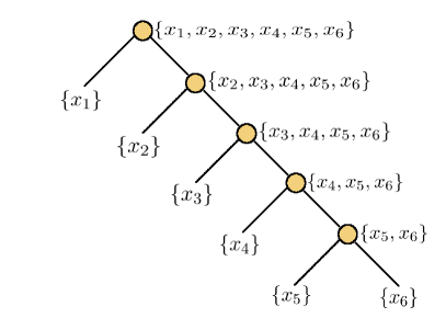
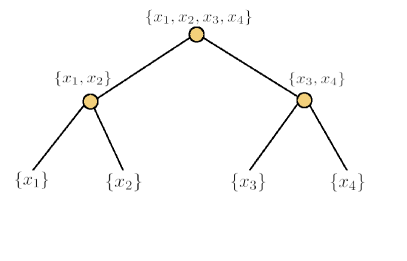
To obtain a series expansion of the multivariate function u(x1,,xd)𝑢subscript𝑥1subscript𝑥𝑑u(x_{1},\ldots,x_{d}) in terms of univariate functions, we apply the bi-orthogonal decomposition method discussed in the previous Section recursively. The way in which the variables are split in each step of the recursive procedure, i.e., the choice of p𝑝p in (8), can be conveniently visualized by binary trees. In Figure 1 we provide two simple examples of such binary trees corresponding to the Tensor-Train (TT) [48] and the Hierarchical Tucker (HT) [26] tensor formats (see also [28, 63], and the references therein).
Refer to caption Refer to caption

Figure 1: Binary trees corresponding to different tensor formats. Left: Tensor Train (TT) decomposition of a six-dimensional function. Right: Hierarchical Tucker (HT) decomposition of a four-dimensional function.

2.1.1 Tensor Train (TT) format

The Tensor-Train format singles out one variable at a time, resulting in a binary tree with depth (d1)𝑑1(d-1) when decomposing d𝑑d-variate functions u(x1,,xd)𝑢subscript𝑥1subscript𝑥𝑑u(x_{1},\ldots,x_{d}) (see Figure 1). This corresponds to the following hierarchical subspace decomposition of the Sobolev space (2)

Hk(Ω)=superscript𝐻𝑘Ωabsent\displaystyle H^{k}(\Omega)= Hk(Ω(1))Hk(Ω(2,,d)),tensor-productsuperscript𝐻𝑘superscriptΩ1superscript𝐻𝑘superscriptΩ2𝑑\displaystyle H^{k}\left(\Omega^{(1)}\right)\otimes H^{k}\left(\Omega^{(2,\ldots,d)}\right),
=\displaystyle= Hk(Ω(1))[Hk(Ω(2))Hk(Ω(3,,d))],tensor-productsuperscript𝐻𝑘superscriptΩ1delimited-[]tensor-productsuperscript𝐻𝑘superscriptΩ2superscript𝐻𝑘superscriptΩ3𝑑\displaystyle H^{k}\left(\Omega^{(1)}\right)\otimes\left[H^{k}\left(\Omega^{(2)}\right)\otimes H^{k}\left(\Omega^{(3,\ldots,d)}\right)\right],
=\displaystyle= Hk(Ω(1))[Hk(Ω(2)){Hk(Ω(3))Hk(Ω(4,,d))}],tensor-productsuperscript𝐻𝑘superscriptΩ1delimited-[]tensor-productsuperscript𝐻𝑘superscriptΩ2tensor-productsuperscript𝐻𝑘superscriptΩ3superscript𝐻𝑘superscriptΩ4𝑑\displaystyle H^{k}\left(\Omega^{(1)}\right)\otimes\left[H^{k}\left(\Omega^{(2)}\right)\otimes\left\{H^{k}\left(\Omega^{(3)}\right)\otimes H^{k}\left(\Omega^{(4,\ldots,d)}\right)\right\}\right]\ ,
\displaystyle\cdots .

in which we diagonalize each tensor product representation using the bi-orthogonal decomposition method. This yields the following TT expansion of the multivariate function u(x1,,xd)𝑢subscript𝑥1subscript𝑥𝑑u(x_{1},\ldots,x_{d})

u𝑢\displaystyle u =i1=1λi1ψi1(1)ψi1(2,,d),absentsuperscriptsubscriptsubscript𝑖11subscript𝜆subscript𝑖1superscriptsubscript𝜓subscript𝑖11superscriptsubscript𝜓subscript𝑖12𝑑\displaystyle=\sum_{i_{1}=1}^{\infty}\lambda_{i_{1}}\psi_{i_{1}}^{(1)}\psi_{i_{1}}^{(2,\ldots,d)}\ , (26)
ψi1(2,,d)superscriptsubscript𝜓subscript𝑖12𝑑\displaystyle\psi_{i_{1}}^{(2,\ldots,d)} =i2=1λi1i2ψi1i2(2)ψi1i2(3,,d),absentsuperscriptsubscriptsubscript𝑖21subscript𝜆subscript𝑖1subscript𝑖2superscriptsubscript𝜓subscript𝑖1subscript𝑖22superscriptsubscript𝜓subscript𝑖1subscript𝑖23𝑑\displaystyle=\sum_{i_{2}=1}^{\infty}\lambda_{i_{1}i_{2}}\psi_{i_{1}i_{2}}^{(2)}\psi_{i_{1}i_{2}}^{(3,\ldots,d)}\ , (27)
\displaystyle\vdots
ψi1ij1(j,,d)superscriptsubscript𝜓subscript𝑖1subscript𝑖𝑗1𝑗𝑑\displaystyle\psi_{i_{1}\cdots i_{j-1}}^{(j,\ldots,d)} =ij=1λi1ijψi1ij(j)ψi1ij(j+1,,d),absentsuperscriptsubscriptsubscript𝑖𝑗1subscript𝜆subscript𝑖1subscript𝑖𝑗superscriptsubscript𝜓subscript𝑖1subscript𝑖𝑗𝑗superscriptsubscript𝜓subscript𝑖1subscript𝑖𝑗𝑗1𝑑\displaystyle=\sum_{i_{j}=1}^{\infty}\lambda_{i_{1}\cdots i_{j}}\psi_{i_{1}\cdots i_{j}}^{(j)}\psi_{i_{1}\cdots i_{j}}^{(j+1,\ldots,d)}\ , (28)
\displaystyle\vdots
ψi1id2(d1,d)superscriptsubscript𝜓subscript𝑖1subscript𝑖𝑑2𝑑1𝑑\displaystyle\psi_{i_{1}\cdots i_{d-2}}^{(d-1,d)} =id1=1λi1id1ψi1id1(d1)ψi1id1(d),absentsuperscriptsubscriptsubscript𝑖𝑑11subscript𝜆subscript𝑖1subscript𝑖𝑑1superscriptsubscript𝜓subscript𝑖1subscript𝑖𝑑1𝑑1superscriptsubscript𝜓subscript𝑖1subscript𝑖𝑑1𝑑\displaystyle=\sum_{i_{d-1}=1}^{\infty}\lambda_{i_{1}\cdots i_{d-1}}\psi_{i_{1}\cdots i_{d-1}}^{(d-1)}\psi_{i_{1}\cdots i_{d-1}}^{(d)}\ , (29)

i.e.,

u=i1=1i2=1id1=1λi1λi1i2λi1id1ψi1(1)ψi1i2(2)ψi1id1(d1)ψi1id1(d).𝑢superscriptsubscriptsubscript𝑖11superscriptsubscriptsubscript𝑖21superscriptsubscriptsubscript𝑖𝑑11subscript𝜆subscript𝑖1subscript𝜆subscript𝑖1subscript𝑖2subscript𝜆subscript𝑖1subscript𝑖𝑑1superscriptsubscript𝜓subscript𝑖11superscriptsubscript𝜓subscript𝑖1subscript𝑖22superscriptsubscript𝜓subscript𝑖1subscript𝑖𝑑1𝑑1superscriptsubscript𝜓subscript𝑖1subscript𝑖𝑑1𝑑u=\sum_{i_{1}=1}^{\infty}\sum_{i_{2}=1}^{\infty}\cdots\sum_{i_{d-1}=1}^{\infty}\lambda_{i_{1}}\lambda_{i_{1}i_{2}}\cdots\lambda_{i_{1}\cdots i_{d-1}}\psi_{i_{1}}^{(1)}\psi_{i_{1}i_{2}}^{(2)}\cdots\psi_{i_{1}\cdots i_{d-1}}^{(d-1)}\psi_{i_{1}\cdots i_{d-1}}^{(d)}. (30)

Each of the bi-orthogonal modes can be obtained by solving a sequence of one-dimensional eigenvalue problems followed by projections. Specifically, the eigenvalue problems are

Luψi1(1)=λi12ψi1(1),Lψi1ik1(k1)ψi1ik(k)=λi1ik2ψi1ik(k),k=2,,d1,formulae-sequencesubscript𝐿𝑢superscriptsubscript𝜓subscript𝑖11superscriptsubscript𝜆subscript𝑖12superscriptsubscript𝜓subscript𝑖11formulae-sequencesubscript𝐿superscriptsubscript𝜓subscript𝑖1subscript𝑖𝑘1𝑘1superscriptsubscript𝜓subscript𝑖1subscript𝑖𝑘𝑘superscriptsubscript𝜆subscript𝑖1subscript𝑖𝑘2superscriptsubscript𝜓subscript𝑖1subscript𝑖𝑘𝑘𝑘2𝑑1L_{u}\psi_{i_{1}}^{(1)}=\lambda_{i_{1}}^{2}\psi_{i_{1}}^{(1)},\qquad L_{\psi_{i_{1}\cdots i_{k-1}}^{(k-1)}}\psi_{i_{1}\cdots i_{k}}^{(k)}=\lambda_{i_{1}\cdots i_{k}}^{2}\psi_{i_{1}\cdots i_{k}}^{(k)},\qquad k=2,\ldots,d-1, (31)

(see Eq. (19)) while the corresponding projections are defined as

ψi1(2,,d)=1λi1u,ψi1(1)Hk(Ω(1)),ψi1ij(j+1,,d)=1λi1iju,ψi1ij(j)Hk(Ω(j+1))j=2,,d1.formulae-sequencesubscriptsuperscript𝜓2𝑑subscript𝑖11subscript𝜆subscript𝑖1subscript𝑢subscriptsuperscript𝜓1subscript𝑖1superscript𝐻𝑘superscriptΩ1formulae-sequencesubscriptsuperscript𝜓𝑗1𝑑subscript𝑖1subscript𝑖𝑗1subscript𝜆subscript𝑖1subscript𝑖𝑗subscript𝑢subscriptsuperscript𝜓𝑗subscript𝑖1subscript𝑖𝑗superscript𝐻𝑘superscriptΩ𝑗1𝑗2𝑑1\psi^{(2,\ldots,d)}_{i_{1}}=\frac{1}{\lambda_{i_{1}}}\langle u,\psi^{(1)}_{i_{1}}\rangle_{H^{k}\left(\Omega^{(1)}\right)},\qquad\psi^{(j+1,\ldots,d)}_{i_{1}\cdots i_{j}}=\frac{1}{\lambda_{i_{1}\cdots i_{j}}}\langle u,\psi^{(j)}_{i_{1}\cdots i_{j}}\rangle_{H^{k}\left(\Omega^{(j+1)}\right)}\qquad j=2,\ldots,d-1. (32)

2.1.2 Hierarchical Tucker (HT) format

The Hierarchical Tucker format splits variables into disjoint subsets of equal size, whenever possible. In the case d𝑑d-variate functions u(x1,,xd)𝑢subscript𝑥1subscript𝑥𝑑u(x_{1},\ldots,x_{d}), where d=2n𝑑superscript2𝑛d=2^{n} for some natural number n𝑛n, the tree is balanced. In general, the Hierarchical Tucker tree is more shallow than a Tensor Train tree for the same number of variables d𝑑d. In fact, the depth of the HT tree for d=2n𝑑superscript2𝑛d=2^{n} is n=log2(d)𝑛subscript2𝑑n=\log_{2}(d), while the corresponding TT tree has depth 2n1superscript2𝑛12^{n}-1. The HT format is based on the following hierarchical decomposition of the Sobolev space Hk(Ω)superscript𝐻𝑘ΩH^{k}(\Omega)

Hk(Ω)=superscript𝐻𝑘Ωabsent\displaystyle H^{k}(\Omega)= Hk(Ω(1,,d/2))Hk(Ω(d/2+1,,d)),tensor-productsuperscript𝐻𝑘superscriptΩ1𝑑2superscript𝐻𝑘superscriptΩ𝑑21𝑑\displaystyle H^{k}\left(\Omega^{(1,\ldots,d/2)}\right)\otimes H^{k}\left(\Omega^{(d/2+1,\ldots,d)}\right),
=\displaystyle= [Hk(Ω(1,,d/4))Hk(Ω(1+d/4,,d/2))][Hk(Ω(d/2+1,,3d/4))Hk(Ω(1+3d/4,,d))],tensor-productdelimited-[]tensor-productsuperscript𝐻𝑘superscriptΩ1𝑑4superscript𝐻𝑘superscriptΩ1𝑑4𝑑2delimited-[]tensor-productsuperscript𝐻𝑘superscriptΩ𝑑213𝑑4superscript𝐻𝑘superscriptΩ13𝑑4𝑑\displaystyle\left[H^{k}\left(\Omega^{(1,\ldots,d/4)}\right)\otimes H^{k}\left(\Omega^{(1+d/4,\ldots,d/2)}\right)\right]\otimes\left[H^{k}\left(\Omega^{(d/2+1,\ldots,3d/4)}\right)\otimes H^{k}\left(\Omega^{(1+3d/4,\ldots,d)}\right)\right]\ ,
\displaystyle\cdots .

As before, we diagonalize each tensor product representation as we proceed splitting variables down the tree. This yields the following sequence of bi-orthogonal decompositions

u𝑢\displaystyle u =i1=1λi1(1,,d/2)ψi1(1,,d/2)ψi1(d/2+1,,d),absentsuperscriptsubscriptsubscript𝑖11superscriptsubscript𝜆subscript𝑖11𝑑2superscriptsubscript𝜓subscript𝑖11𝑑2superscriptsubscript𝜓subscript𝑖1𝑑21𝑑\displaystyle=\sum_{i_{1}=1}^{\infty}\lambda_{i_{1}}^{(1,\ldots,d/2)}\psi_{i_{1}}^{(1,\ldots,d/2)}\psi_{i_{1}}^{(d/2+1,\ldots,d)}\ , (33)
ψi1(1,,d/2)superscriptsubscript𝜓subscript𝑖11𝑑2\displaystyle\psi_{i_{1}}^{(1,\ldots,d/2)} =i2=1λi1i2(1,,d/4)ψi1i2(1,,d/4)ψi1i2(d/4+1,,d/2),absentsuperscriptsubscriptsubscript𝑖21superscriptsubscript𝜆subscript𝑖1subscript𝑖21𝑑4superscriptsubscript𝜓subscript𝑖1subscript𝑖21𝑑4superscriptsubscript𝜓subscript𝑖1subscript𝑖2𝑑41𝑑2\displaystyle=\sum_{i_{2}=1}^{\infty}\lambda_{i_{1}i_{2}}^{(1,\ldots,d/4)}\psi_{i_{1}i_{2}}^{(1,\ldots,d/4)}\psi_{i_{1}i_{2}}^{(d/4+1,\ldots,d/2)}\ , (34)
ψi1(d/2+1,,d)superscriptsubscript𝜓subscript𝑖1𝑑21𝑑\displaystyle\psi_{i_{1}}^{(d/2+1,\ldots,d)} =i2=1λi1i2(d/2+1,,3d/4)ψi1i2(d/2+1,,3d/4)ψi1i2(3d/4+1,,d),absentsuperscriptsubscriptsubscript𝑖21superscriptsubscript𝜆subscript𝑖1subscript𝑖2𝑑213𝑑4superscriptsubscript𝜓subscript𝑖1subscript𝑖2𝑑213𝑑4superscriptsubscript𝜓subscript𝑖1subscript𝑖23𝑑41𝑑\displaystyle=\sum_{i_{2}=1}^{\infty}\lambda_{i_{1}i_{2}}^{(d/2+1,\ldots,3d/4)}\psi_{i_{1}i_{2}}^{(d/2+1,\ldots,3d/4)}\psi_{i_{1}i_{2}}^{(3d/4+1,\ldots,d)}\ , (35)
\displaystyle\vdots
ψi1in1(1,2)superscriptsubscript𝜓subscript𝑖1subscript𝑖𝑛112\displaystyle\psi_{i_{1}\cdots i_{n-1}}^{(1,2)} =in=1λi1in(1)ψi1in(1)ψi1in(2),absentsuperscriptsubscriptsubscript𝑖𝑛1superscriptsubscript𝜆subscript𝑖1subscript𝑖𝑛1superscriptsubscript𝜓subscript𝑖1subscript𝑖𝑛1superscriptsubscript𝜓subscript𝑖1subscript𝑖𝑛2\displaystyle=\sum_{i_{n}=1}^{\infty}\lambda_{i_{1}\cdots i_{n}}^{(1)}\psi_{i_{1}\cdots i_{n}}^{(1)}\psi_{i_{1}\cdots i_{n}}^{(2)}\ , (36)
\displaystyle\vdots
ψi1in1(d1,d)superscriptsubscript𝜓subscript𝑖1subscript𝑖𝑛1𝑑1𝑑\displaystyle\psi_{i_{1}\cdots i_{n-1}}^{(d-1,d)} =in=1λi1in(d1)ψi1in(d1)ψi1in(d),absentsuperscriptsubscriptsubscript𝑖𝑛1superscriptsubscript𝜆subscript𝑖1subscript𝑖𝑛𝑑1superscriptsubscript𝜓subscript𝑖1subscript𝑖𝑛𝑑1superscriptsubscript𝜓subscript𝑖1subscript𝑖𝑛𝑑\displaystyle=\sum_{i_{n}=1}^{\infty}\lambda_{i_{1}\cdots i_{n}}^{(d-1)}\psi_{i_{1}\cdots i_{n}}^{(d-1)}\psi_{i_{1}\cdots i_{n}}^{(d)}\ , (37)

and the expansion

u=i1=1in=1λi1(1,,d2)λi1in(d1)ψi1in(1)ψi1in(2)ψi1in(d).𝑢superscriptsubscriptsubscript𝑖11superscriptsubscriptsubscript𝑖𝑛1superscriptsubscript𝜆subscript𝑖11𝑑2superscriptsubscript𝜆subscript𝑖1subscript𝑖𝑛𝑑1superscriptsubscript𝜓subscript𝑖1subscript𝑖𝑛1superscriptsubscript𝜓subscript𝑖1subscript𝑖𝑛2superscriptsubscript𝜓subscript𝑖1subscript𝑖𝑛𝑑u=\sum_{i_{1}=1}^{\infty}\cdots\sum_{i_{n}=1}^{\infty}\lambda_{i_{1}}^{(1,\ldots,\frac{d}{2})}\cdots\lambda_{i_{1}\cdots i_{n}}^{(d-1)}\psi_{i_{1}\cdots i_{n}}^{(1)}\psi_{i_{1}\cdots i_{n}}^{(2)}\cdots\psi_{i_{1}\cdots i_{n}}^{(d)}. (38)

Similar to the TT format, a sequence of eigenfunction problems followed by projections are used to obtain the modes spanning the hierarchical subspaces. However, in the HT case the eigenfunction problems are higher dimensional and not tractable for large d𝑑d.

Remark

Clearly, we may decompose a multivariate function u(x1,,xd)𝑢subscript𝑥1subscript𝑥𝑑u(x_{1},\ldots,x_{d}) by splitting variables in various ways at different levels of the decompositions. Any binary tree which has leaves containing one index leads to a series expansion in terms of functions of one spatial variable. Separable Hilbert spaces defined on a Cartesian product of one-dimensional domains always allow such reduction.

2.2 Error analysis

In this Section we develop an error analysis for the recursive biorthogonal decomposition we discussed in Section 2.1. To this end we first state a Lemma which will be useful in Section 2.4 for establishing a thresholding criterion to truncate the infinite sums in (30) and (38).

Lemma 2.1.

If uHk(Ω)𝑢superscript𝐻𝑘Ωu\in H^{k}(\Omega) admits the bi-orthogonal expansion

u=i=1λiψi(1,,p)ψi(p+1,,d)p{2,,d1},formulae-sequence𝑢superscriptsubscript𝑖1subscript𝜆𝑖subscriptsuperscript𝜓1𝑝𝑖subscriptsuperscript𝜓𝑝1𝑑𝑖𝑝2𝑑1u=\sum_{i=1}^{\infty}\lambda_{i}\psi^{(1,\ldots,p)}_{i}\psi^{(p+1,\ldots,d)}_{i}\qquad p\in\{2,\ldots,d-1\}\ , (39)

then i=1λi2=uHk(Ω)2superscriptsubscript𝑖1superscriptsubscript𝜆𝑖2subscriptsuperscriptnorm𝑢2superscript𝐻𝑘Ω\displaystyle\sum_{i=1}^{\infty}\lambda_{i}^{2}=\|u\|^{2}_{H^{k}(\Omega)}.

Proof.

This result follows immediately from the orthonormality of the modes ψi(1,,p)superscriptsubscript𝜓𝑖1𝑝\psi_{i}^{(1,\ldots,p)} and ψi(p+1,,d)superscriptsubscript𝜓𝑖𝑝1𝑑\psi_{i}^{(p+1,\ldots,d)} relative to the inner products (9)-(10).

Next, we analyze the error in the Hk(Ω)superscript𝐻𝑘ΩH^{k}(\Omega) norm between the Tensor Train series expansion (30) and the truncated expansion

u~=i1=1r1i2=1r2(i1)id1=1rd1(i1,,id2)λi1λi1id1ψi1(1)ψi1i2(2)ψi1id1(d1)ψi1id1(d),~𝑢superscriptsubscriptsubscript𝑖11subscript𝑟1superscriptsubscriptsubscript𝑖21subscript𝑟2subscript𝑖1superscriptsubscriptsubscript𝑖𝑑11subscript𝑟𝑑1subscript𝑖1subscript𝑖𝑑2subscript𝜆subscript𝑖1subscript𝜆subscript𝑖1subscript𝑖𝑑1superscriptsubscript𝜓subscript𝑖11superscriptsubscript𝜓subscript𝑖1subscript𝑖22superscriptsubscript𝜓subscript𝑖1subscript𝑖𝑑1𝑑1superscriptsubscript𝜓subscript𝑖1subscript𝑖𝑑1𝑑\tilde{u}=\sum_{i_{1}=1}^{r_{1}}\sum_{i_{2}=1}^{r_{2}(i_{1})}\cdots\sum_{i_{d-1}=1}^{r_{d-1}(i_{1},\ldots,i_{d-2})}\lambda_{i_{1}}\cdots\lambda_{i_{1}\cdots i_{d-1}}\psi_{i_{1}}^{(1)}\psi_{i_{1}i_{2}}^{(2)}\cdots\psi_{i_{1}\cdots i_{d-1}}^{(d-1)}\psi_{i_{1}\cdots i_{d-1}}^{(d)}\ , (40)

where r1,r2,,rd1subscript𝑟1subscript𝑟2subscript𝑟𝑑1r_{1},r_{2},\ldots,r_{d-1} are truncation ranks. To simplify indexing and array bounds for truncated TT expansions such as (40), we will omit the array indices in the rank arrays and write, e.g., ψi1ik(j1,,jp),k=1,,rkformulae-sequencesubscriptsuperscript𝜓subscript𝑗1subscript𝑗𝑝subscript𝑖1subscript𝑖𝑘𝑘1subscript𝑟𝑘\psi^{(j_{1},\ldots,j_{p})}_{i_{1}\cdots i_{k}},\ k=1,\ldots,r_{k} instead of k=1,,rk(i1,,ik1)𝑘1subscript𝑟𝑘subscript𝑖1subscript𝑖𝑘1k=1,\ldots,r_{k}(i_{1},\ldots,i_{k-1}), since the rank array indices are clear from the subscripts of the mode ψi1ik(j1,,jp)subscriptsuperscript𝜓subscript𝑗1subscript𝑗𝑝subscript𝑖1subscript𝑖𝑘\psi^{(j_{1},\ldots,j_{p})}_{i_{1}\cdots i_{k}}. In this simplified notation, the truncated TT expansion (40) can be written as

u~(1,,d)=i1=1r1i2=1r2id1=1rd1λi1λi1id1ψi1(1)ψi1i2(2)ψi1id1(d1)ψi1id1(d).superscript~𝑢1𝑑superscriptsubscriptsubscript𝑖11subscript𝑟1superscriptsubscriptsubscript𝑖21subscript𝑟2superscriptsubscriptsubscript𝑖𝑑11subscript𝑟𝑑1subscript𝜆subscript𝑖1subscript𝜆subscript𝑖1subscript𝑖𝑑1superscriptsubscript𝜓subscript𝑖11superscriptsubscript𝜓subscript𝑖1subscript𝑖22superscriptsubscript𝜓subscript𝑖1subscript𝑖𝑑1𝑑1superscriptsubscript𝜓subscript𝑖1subscript𝑖𝑑1𝑑\tilde{u}^{(1,\ldots,d)}=\sum_{i_{1}=1}^{r_{1}}\sum_{i_{2}=1}^{r_{2}}\cdots\sum_{i_{d-1}=1}^{r_{d-1}}\lambda_{i_{1}}\cdots\lambda_{i_{1}\cdots i_{d-1}}\psi_{i_{1}}^{(1)}\psi_{i_{1}i_{2}}^{(2)}\cdots\psi_{i_{1}\cdots i_{d-1}}^{(d-1)}\psi_{i_{1}\cdots i_{d-1}}^{(d)}. (41)
Proposition 2.1.

Let uHk(Ω)𝑢superscript𝐻𝑘Ωu\in H^{k}(\Omega). The error incurred by truncating the infinite expanion (30) to the finite expansion (41) is given by

uu~Hk(Ω)2=subscriptsuperscriptnorm𝑢~𝑢2superscript𝐻𝑘Ωabsent\displaystyle\|u-\tilde{u}\|^{2}_{H^{k}(\Omega)}= i1=r1+1λi12+i1=1r1i2=r2+1λi12λi1i22+superscriptsubscriptsubscript𝑖1subscript𝑟11superscriptsubscript𝜆subscript𝑖12superscriptsubscriptsubscript𝑖11subscript𝑟1superscriptsubscriptsubscript𝑖2subscript𝑟21superscriptsubscript𝜆subscript𝑖12superscriptsubscript𝜆subscript𝑖1subscript𝑖22\displaystyle\sum_{i_{1}=r_{1}+1}^{\infty}\lambda_{i_{1}}^{2}+\sum_{i_{1}=1}^{r_{1}}\sum_{i_{2}=r_{2}+1}^{\infty}\lambda_{i_{1}}^{2}\lambda_{i_{1}i_{2}}^{2}+\cdots (42)
+i1=1r1i2=1r2id2=1rd2id1=rd1+1λi12λi1i22λi1id12.superscriptsubscriptsubscript𝑖11subscript𝑟1superscriptsubscriptsubscript𝑖21subscript𝑟2superscriptsubscriptsubscript𝑖𝑑21subscript𝑟𝑑2superscriptsubscriptsubscript𝑖𝑑1subscript𝑟𝑑11superscriptsubscript𝜆subscript𝑖12superscriptsubscript𝜆subscript𝑖1subscript𝑖22superscriptsubscript𝜆subscript𝑖1subscript𝑖𝑑12\displaystyle+\sum_{i_{1}=1}^{r_{1}}\sum_{i_{2}=1}^{r_{2}}\cdots\sum_{i_{d-2}=1}^{r_{d-2}}\sum_{i_{d-1}=r_{d-1}+1}^{\infty}\lambda_{i_{1}}^{2}\lambda_{i_{1}i_{2}}^{2}\cdots\lambda_{i_{1}\cdots i_{d-1}}^{2}.
Proof.

Let us rewrite (30) as

u=i1=1λi1ψi1(1)i2=1λi1i2ψi1i2(2)id1=1λi1id1ψi1id1(d1)ψi1id1(d)𝑢superscriptsubscriptsubscript𝑖11subscript𝜆subscript𝑖1superscriptsubscript𝜓subscript𝑖11superscriptsubscriptsubscript𝑖21subscript𝜆subscript𝑖1subscript𝑖2superscriptsubscript𝜓subscript𝑖1subscript𝑖22superscriptsubscriptsubscript𝑖𝑑11subscript𝜆subscript𝑖1subscript𝑖𝑑1superscriptsubscript𝜓subscript𝑖1subscript𝑖𝑑1𝑑1superscriptsubscript𝜓subscript𝑖1subscript𝑖𝑑1𝑑u=\sum_{i_{1}=1}^{\infty}\lambda_{i_{1}}\psi_{i_{1}}^{(1)}\sum_{i_{2}=1}^{\infty}\lambda_{i_{1}i_{2}}\psi_{i_{1}i_{2}}^{(2)}\cdots\sum_{i_{d-1}=1}^{\infty}\lambda_{i_{1}\cdots i_{d-1}}\psi_{i_{1}\cdots i_{d-1}}^{(d-1)}\psi_{i_{1}\cdots i_{d-1}}^{(d)} (43)

and split each infinite sum into the superimposition of a finite sum and an infinite sum, i.e.,

u=𝑢absent\displaystyle u= (i1=1r1λi1ψi1(1)+i1=r1+1λi1ψi1(1))(i2=1r2λi1i2ψi1i2(2)+i2=r2+1λi1i2ψi1i2(2))superscriptsubscriptsubscript𝑖11subscript𝑟1subscript𝜆subscript𝑖1superscriptsubscript𝜓subscript𝑖11superscriptsubscriptsubscript𝑖1subscript𝑟11subscript𝜆subscript𝑖1superscriptsubscript𝜓subscript𝑖11superscriptsubscriptsubscript𝑖21subscript𝑟2subscript𝜆subscript𝑖1subscript𝑖2superscriptsubscript𝜓subscript𝑖1subscript𝑖22superscriptsubscriptsubscript𝑖2subscript𝑟21subscript𝜆subscript𝑖1subscript𝑖2superscriptsubscript𝜓subscript𝑖1subscript𝑖22\displaystyle\left(\sum_{i_{1}=1}^{r_{1}}\lambda_{i_{1}}\psi_{i_{1}}^{(1)}+\sum_{i_{1}=r_{1}+1}^{\infty}\lambda_{i_{1}}\psi_{i_{1}}^{(1)}\right)\left(\sum_{i_{2}=1}^{r_{2}}\lambda_{i_{1}i_{2}}\psi_{i_{1}i_{2}}^{(2)}+\sum_{i_{2}=r_{2}+1}^{\infty}\lambda_{i_{1}i_{2}}\psi_{i_{1}i_{2}}^{(2)}\right)\cdots (44)
(id1=1rd1λi1id1ψi1id1(d1)ψi1id1(d)+id1=rd1+1λi1id1ψi1id1(d1)ψi1id1(d)).superscriptsubscriptsubscript𝑖𝑑11subscript𝑟𝑑1subscript𝜆subscript𝑖1subscript𝑖𝑑1superscriptsubscript𝜓subscript𝑖1subscript𝑖𝑑1𝑑1superscriptsubscript𝜓subscript𝑖1subscript𝑖𝑑1𝑑superscriptsubscriptsubscript𝑖𝑑1subscript𝑟𝑑11subscript𝜆subscript𝑖1subscript𝑖𝑑1superscriptsubscript𝜓subscript𝑖1subscript𝑖𝑑1𝑑1superscriptsubscript𝜓subscript𝑖1subscript𝑖𝑑1𝑑\displaystyle\cdots\left(\sum_{i_{d-1}=1}^{r_{d-1}}\lambda_{i_{1}\cdots i_{d-1}}\psi_{i_{1}\cdots i_{d-1}}^{(d-1)}\psi_{i_{1}\cdots i_{d-1}}^{(d)}+\sum_{i_{d-1}=r_{d-1}+1}^{\infty}\lambda_{i_{1}\cdots i_{d-1}}\psi_{i_{1}\cdots i_{d-1}}^{(d-1)}\psi_{i_{1}\cdots i_{d-1}}^{(d)}\right).

Expanding the products in (44) yields the following expression

u=𝑢absent\displaystyle u= i1=1r1i2=1r2id1=1rd1λi1λi1id1ψi1(1)ψi1id1(d1)ψi1id1(d)superscriptsubscriptsubscript𝑖11subscript𝑟1superscriptsubscriptsubscript𝑖21subscript𝑟2superscriptsubscriptsubscript𝑖𝑑11subscript𝑟𝑑1subscript𝜆subscript𝑖1subscript𝜆subscript𝑖1subscript𝑖𝑑1subscriptsuperscript𝜓1subscript𝑖1subscriptsuperscript𝜓𝑑1subscript𝑖1subscript𝑖𝑑1subscriptsuperscript𝜓𝑑subscript𝑖1subscript𝑖𝑑1\displaystyle\sum_{i_{1}=1}^{r_{1}}\sum_{i_{2}=1}^{r_{2}}\cdots\sum_{i_{d-1}=1}^{r_{d-1}}\lambda_{i_{1}}\cdots\lambda_{i_{1}\cdots i_{d-1}}\psi^{(1)}_{i_{1}}\cdots\psi^{(d-1)}_{i_{1}\cdots i_{d-1}}\psi^{(d)}_{i_{1}\cdots i_{d-1}} (45)
+i1=r1+1i2=1id1=1λi1λi1id1ψi1(1)ψi1id1(d1)ψi1id1(d)superscriptsubscriptsubscript𝑖1subscript𝑟11superscriptsubscriptsubscript𝑖21superscriptsubscriptsubscript𝑖𝑑11subscript𝜆subscript𝑖1subscript𝜆subscript𝑖1subscript𝑖𝑑1subscriptsuperscript𝜓1subscript𝑖1subscriptsuperscript𝜓𝑑1subscript𝑖1subscript𝑖𝑑1subscriptsuperscript𝜓𝑑subscript𝑖1subscript𝑖𝑑1\displaystyle+\sum_{i_{1}=r_{1}+1}^{\infty}\sum_{i_{2}=1}^{\infty}\cdots\sum_{i_{d-1}=1}^{\infty}\lambda_{i_{1}}\cdots\lambda_{i_{1}\cdots i_{d-1}}\psi^{(1)}_{i_{1}}\cdots\psi^{(d-1)}_{i_{1}\cdots i_{d-1}}\psi^{(d)}_{i_{1}\cdots i_{d-1}}
+i1=1r1i2=r2+1i3=1id1=1λi1λi1id1ψi1(1)ψi1id1(d1)ψi1id1(d)superscriptsubscriptsubscript𝑖11subscript𝑟1superscriptsubscriptsubscript𝑖2subscript𝑟21superscriptsubscriptsubscript𝑖31superscriptsubscriptsubscript𝑖𝑑11subscript𝜆subscript𝑖1subscript𝜆subscript𝑖1subscript𝑖𝑑1subscriptsuperscript𝜓1subscript𝑖1subscriptsuperscript𝜓𝑑1subscript𝑖1subscript𝑖𝑑1subscriptsuperscript𝜓𝑑subscript𝑖1subscript𝑖𝑑1\displaystyle+\sum_{i_{1}=1}^{r_{1}}\sum_{i_{2}=r_{2}+1}^{\infty}\sum_{i_{3}=1}^{\infty}\cdots\sum_{i_{d-1}=1}^{\infty}\lambda_{i_{1}}\cdots\lambda_{i_{1}\cdots i_{d-1}}\psi^{(1)}_{i_{1}}\cdots\psi^{(d-1)}_{i_{1}\cdots i_{d-1}}\psi^{(d)}_{i_{1}\cdots i_{d-1}}
+i1=1r1i2=1r2i3=r3+1i4=1id1=1λi1λi1id1ψi1(1)ψi1id1(d1)ψi1id1(d)superscriptsubscriptsubscript𝑖11subscript𝑟1superscriptsubscriptsubscript𝑖21subscript𝑟2superscriptsubscriptsubscript𝑖3subscript𝑟31superscriptsubscriptsubscript𝑖41superscriptsubscriptsubscript𝑖𝑑11subscript𝜆subscript𝑖1subscript𝜆subscript𝑖1subscript𝑖𝑑1subscriptsuperscript𝜓1subscript𝑖1subscriptsuperscript𝜓𝑑1subscript𝑖1subscript𝑖𝑑1subscriptsuperscript𝜓𝑑subscript𝑖1subscript𝑖𝑑1\displaystyle+\sum_{i_{1}=1}^{r_{1}}\sum_{i_{2}=1}^{r_{2}}\sum_{i_{3}=r_{3}+1}^{\infty}\sum_{i_{4}=1}^{\infty}\cdots\sum_{i_{d-1}=1}^{\infty}\lambda_{i_{1}}\cdots\lambda_{i_{1}\cdots i_{d-1}}\psi^{(1)}_{i_{1}}\cdots\psi^{(d-1)}_{i_{1}\cdots i_{d-1}}\psi^{(d)}_{i_{1}\cdots i_{d-1}}
\displaystyle\hskip 56.9055pt\vdots
+i1=1r1i2=1r2id2=1rd2id1=rd1+1λi1λi1id1ψi1(1)ψi1id1(d1)ψi1id1(d).superscriptsubscriptsubscript𝑖11subscript𝑟1superscriptsubscriptsubscript𝑖21subscript𝑟2superscriptsubscriptsubscript𝑖𝑑21subscript𝑟𝑑2superscriptsubscriptsubscript𝑖𝑑1subscript𝑟𝑑11subscript𝜆subscript𝑖1subscript𝜆subscript𝑖1subscript𝑖𝑑1subscriptsuperscript𝜓1subscript𝑖1subscriptsuperscript𝜓𝑑1subscript𝑖1subscript𝑖𝑑1subscriptsuperscript𝜓𝑑subscript𝑖1subscript𝑖𝑑1\displaystyle+\sum_{i_{1}=1}^{r_{1}}\sum_{i_{2}=1}^{r_{2}}\cdots\sum_{i_{d-2}=1}^{r_{d-2}}\sum_{i_{d-1}=r_{d-1}+1}^{\infty}\lambda_{i_{1}}\cdots\lambda_{i_{1}\cdots i_{d-1}}\psi^{(1)}_{i_{1}}\cdots\psi^{(d-1)}_{i_{1}\cdots i_{d-1}}\psi^{(d)}_{i_{1}\cdots i_{d-1}}.

Using the orthogonality of each set of modes we obtain

uu~Hk(Ω)2=superscriptsubscriptnorm𝑢~𝑢superscript𝐻𝑘Ω2absent\displaystyle\|u-\tilde{u}\|_{H^{k}(\Omega)}^{2}= i1=r1+1i2=1id1=1λi1λi1id1ψi1(1)ψi1id1(d1)ψi1id1(d)Hk(Ω)2superscriptsubscriptsubscript𝑖1subscript𝑟11superscriptsubscriptsubscript𝑖21superscriptsubscriptsubscript𝑖𝑑11subscript𝜆subscript𝑖1subscript𝜆subscript𝑖1subscript𝑖𝑑1superscriptsubscriptnormsubscriptsuperscript𝜓1subscript𝑖1subscriptsuperscript𝜓𝑑1subscript𝑖1subscript𝑖𝑑1subscriptsuperscript𝜓𝑑subscript𝑖1subscript𝑖𝑑1superscript𝐻𝑘Ω2\displaystyle\sum_{i_{1}=r_{1}+1}^{\infty}\sum_{i_{2}=1}^{\infty}\cdots\sum_{i_{d-1}=1}^{\infty}\lambda_{i_{1}}\cdots\lambda_{i_{1}\cdots i_{d-1}}\|\psi^{(1)}_{i_{1}}\cdots\psi^{(d-1)}_{i_{1}\cdots i_{d-1}}\psi^{(d)}_{i_{1}\cdots i_{d-1}}\|_{H^{k}(\Omega)}^{2}
+\displaystyle+ i1=1r1i2=r2+1i3=1id1=1λi1λi1id1ψi1(1)ψi1id1(d1)ψi1id1(d)Hk(Ω)2superscriptsubscriptsubscript𝑖11subscript𝑟1superscriptsubscriptsubscript𝑖2subscript𝑟21superscriptsubscriptsubscript𝑖31superscriptsubscriptsubscript𝑖𝑑11subscript𝜆subscript𝑖1subscript𝜆subscript𝑖1subscript𝑖𝑑1superscriptsubscriptnormsubscriptsuperscript𝜓1subscript𝑖1subscriptsuperscript𝜓𝑑1subscript𝑖1subscript𝑖𝑑1subscriptsuperscript𝜓𝑑subscript𝑖1subscript𝑖𝑑1superscript𝐻𝑘Ω2\displaystyle\sum_{i_{1}=1}^{r_{1}}\sum_{i_{2}=r_{2}+1}^{\infty}\sum_{i_{3}=1}^{\infty}\cdots\sum_{i_{d-1}=1}^{\infty}\lambda_{i_{1}}\cdots\lambda_{i_{1}\cdots i_{d-1}}\|\psi^{(1)}_{i_{1}}\cdots\psi^{(d-1)}_{i_{1}\cdots i_{d-1}}\psi^{(d)}_{i_{1}\cdots i_{d-1}}\|_{H^{k}(\Omega)}^{2}
+\displaystyle+ i1=1r1i2=1r2i3=r3+1i4=1id1=1λi1λi1id1ψi1(1)ψi1id1(d1)ψi1id1(d)Hk(Ω)2superscriptsubscriptsubscript𝑖11subscript𝑟1superscriptsubscriptsubscript𝑖21subscript𝑟2superscriptsubscriptsubscript𝑖3subscript𝑟31superscriptsubscriptsubscript𝑖41superscriptsubscriptsubscript𝑖𝑑11subscript𝜆subscript𝑖1subscript𝜆subscript𝑖1subscript𝑖𝑑1superscriptsubscriptnormsubscriptsuperscript𝜓1subscript𝑖1subscriptsuperscript𝜓𝑑1subscript𝑖1subscript𝑖𝑑1subscriptsuperscript𝜓𝑑subscript𝑖1subscript𝑖𝑑1superscript𝐻𝑘Ω2\displaystyle\sum_{i_{1}=1}^{r_{1}}\sum_{i_{2}=1}^{r_{2}}\sum_{i_{3}=r_{3}+1}^{\infty}\sum_{i_{4}=1}^{\infty}\cdots\sum_{i_{d-1}=1}^{\infty}\lambda_{i_{1}}\cdots\lambda_{i_{1}\cdots i_{d-1}}\|\psi^{(1)}_{i_{1}}\cdots\psi^{(d-1)}_{i_{1}\cdots i_{d-1}}\psi^{(d)}_{i_{1}\cdots i_{d-1}}\|_{H^{k}(\Omega)}^{2}
\displaystyle\hskip 56.9055pt\vdots
+i1=1r1i2=1r2id2=1rd2id1=rd1+1λi1λi1id1ψi1(1)ψi1id1(d1)ψi1id1(d)Hk(Ω)2.superscriptsubscriptsubscript𝑖11subscript𝑟1superscriptsubscriptsubscript𝑖21subscript𝑟2superscriptsubscriptsubscript𝑖𝑑21subscript𝑟𝑑2superscriptsubscriptsubscript𝑖𝑑1subscript𝑟𝑑11subscript𝜆subscript𝑖1subscript𝜆subscript𝑖1subscript𝑖𝑑1superscriptsubscriptnormsubscriptsuperscript𝜓1subscript𝑖1subscriptsuperscript𝜓𝑑1subscript𝑖1subscript𝑖𝑑1subscriptsuperscript𝜓𝑑subscript𝑖1subscript𝑖𝑑1superscript𝐻𝑘Ω2\displaystyle+\sum_{i_{1}=1}^{r_{1}}\sum_{i_{2}=1}^{r_{2}}\cdots\sum_{i_{d-2}=1}^{r_{d-2}}\sum_{i_{d-1}=r_{d-1}+1}^{\infty}\lambda_{i_{1}}\cdots\lambda_{i_{1}\cdots i_{d-1}}\|\psi^{(1)}_{i_{1}}\cdots\psi^{(d-1)}_{i_{1}\cdots i_{d-1}}\psi^{(d)}_{i_{1}\cdots i_{d-1}}\|_{H^{k}(\Omega)}^{2}.

i.e.,

uu~Hk(Ω)2=superscriptsubscriptnorm𝑢~𝑢superscript𝐻𝑘Ω2absent\displaystyle\|u-\tilde{u}\|_{H^{k}(\Omega)}^{2}= i1=r1+1λi12+i1=1r1i2=r2+1λi12λi1i22+superscriptsubscriptsubscript𝑖1subscript𝑟11superscriptsubscript𝜆subscript𝑖12superscriptsubscriptsubscript𝑖11subscript𝑟1superscriptsubscriptsubscript𝑖2subscript𝑟21superscriptsubscript𝜆subscript𝑖12superscriptsubscript𝜆subscript𝑖1subscript𝑖22\displaystyle\sum_{i_{1}=r_{1}+1}^{\infty}\lambda_{i_{1}}^{2}+\sum_{i_{1}=1}^{r_{1}}\sum_{i_{2}=r_{2}+1}^{\infty}\lambda_{i_{1}}^{2}\lambda_{i_{1}i_{2}}^{2}+\cdots
+i1=1r1i2=1r2id2=1rd2id1=rd1+1λi12λi1i22λi1id12.superscriptsubscriptsubscript𝑖11subscript𝑟1superscriptsubscriptsubscript𝑖21subscript𝑟2superscriptsubscriptsubscript𝑖𝑑21subscript𝑟𝑑2superscriptsubscriptsubscript𝑖𝑑1subscript𝑟𝑑11superscriptsubscript𝜆subscript𝑖12superscriptsubscript𝜆subscript𝑖1subscript𝑖22superscriptsubscript𝜆subscript𝑖1subscript𝑖𝑑12\displaystyle+\sum_{i_{1}=1}^{r_{1}}\sum_{i_{2}=1}^{r_{2}}\cdots\sum_{i_{d-2}=1}^{r_{d-2}}\sum_{i_{d-1}=r_{d-1}+1}^{\infty}\lambda_{i_{1}}^{2}\lambda_{i_{1}i_{2}}^{2}\cdots\lambda_{i_{1}\cdots i_{d-1}}^{2}.

Remark

Proposition 2.1 can be generalized to tensor formats corresponding to arbitrary binary trees, e.g., the HT format (38). In some sense, the equality (42) represents the infinite-dimensional version of well-known finite-dimensional results which bound the overall squared approximation error of multilinear singular value decompositions in the 2-norm by the sum (over the whole tree) of squares of deleted singular values. These types of results were first proven by De Lathauwer et al. in [41], and later generalized by Grasedyck [24] (see also Schneider and Uschmajew [58]).

Remark

Recent error estimates by Griebel and Li [27] on the decay rate of singular values allow us to develop sharp upper bounds for (42) depending only on the multivariate rank, the smoothness of the function u(x1,,xd)𝑢subscript𝑥1subscript𝑥𝑑u(x_{1},\ldots,x_{d}) and other computable quantities. To obtain such estimates, it is sufficient to bound each eigenvalue λi12superscriptsubscript𝜆subscript𝑖12\lambda_{i_{1}}^{2}, λi1i22superscriptsubscript𝜆subscript𝑖1subscript𝑖22\lambda_{i_{1}i_{2}}^{2}, etc., with the corresponding sharp upper bound recently obtained in [27].

2.3 Computational aspects of TT and HT series expansions

To compute a recursive bi-orthogonal decomposition of the multivariate function u(x1,xd)𝑢subscript𝑥1subscript𝑥𝑑u(x_{1},\ldots x_{d}) we first need to identify the self-adjoint operator (19) (or (17)) at each level of the binary tree (see Figure 1). In other words, we need to compute the kernel (20), (or (18)) and then solve the corresponding eigenfunction problem. In the HT tensor format, computing such kernel requires evaluating a multivariate integral of dimension d/2𝑑2d/2 (at the first level of the tree) and then solving an eigenfunction problem of dimension d/2𝑑2d/2, which can be extremely challenging when d𝑑d is large. In the TT tensor format, this problem can be mitigated substantially. In fact, at the first level of the TT tree we have that the kernel of Lusubscript𝐿𝑢L_{u} is a (d1)𝑑1(d-1)-dimensional integral which can be evaluated, e.g., by using Quasi-Monte Carlo or more general lattice cubature rules [21]. The corresponding eigenvalue problem (31) and the projection (32) are both one-dimensional. From a numerical viewpoint, this is extremely advantageous, as we can accurately solve one dimensional eigenvalue problems in a collocation or a Galerkin setting at a low computational cost, once the kernels of the operators in (31) are available.

2.4 Thresholding hierarchical bi-orthogonal series expansions

In this Section we develop a new thresholding criterion to truncate the series expansion (30) and (38) to finite rank. To this end, we first notice that the amplitude of each term in the series is represented by products of eigenvalues from each level of the binary tree, since all eigenmodes are normalized. With this in mind, it is clear that a reasonable criterion to truncate the bi-orthogonal series expansion (30) (or (38)) to finite rank is to ensure that each of these eigenvalue products remains above a specified threshold σ𝜎\sigma. Hereafter, we develop this criterion for the TT format (30). The same technique can be applied to any other tensor format. We begin by setting some threshold value σ𝜎\sigma for which we enforce λi1λi1i2λi1id1σsubscript𝜆subscript𝑖1subscript𝜆subscript𝑖1subscript𝑖2subscript𝜆subscript𝑖1subscript𝑖𝑑1𝜎\lambda_{i_{1}}\lambda_{i_{1}i_{2}}\cdots\lambda_{i_{1}\cdots i_{d-1}}\geq\sigma. In the first level of the TT tree (Figure (1)), i.e., Eq. (26), we keep all modes with eigenvalues λi1σsubscript𝜆subscript𝑖1𝜎\lambda_{i_{1}}\geq\sigma, of which there will be a finite number r1subscript𝑟1r_{1} because of property (23). Then we proceed to the second level of the TT tree and decompose ψi1(2,,d)subscriptsuperscript𝜓2𝑑subscript𝑖1\psi^{(2,\ldots,d)}_{i_{1}} (1i1r11subscript𝑖1subscript𝑟11\leq i_{1}\leq r_{1}) as in (27). Here we set new thresholds σi1=σ/λi1subscript𝜎subscript𝑖1𝜎subscript𝜆subscript𝑖1\sigma_{i_{1}}=\sigma/\lambda_{i_{1}} and keep all modes ψi1i2(2),ψi1i2(3,,d)subscriptsuperscript𝜓2subscript𝑖1subscript𝑖2subscriptsuperscript𝜓3𝑑subscript𝑖1subscript𝑖2\psi^{(2)}_{i_{1}i_{2}},\psi^{(3,\ldots,d)}_{i_{1}i_{2}} with eigenvalues λi1i2σi1subscript𝜆subscript𝑖1subscript𝑖2subscript𝜎subscript𝑖1\lambda_{i_{1}i_{2}}\geq\sigma_{i_{1}}. Proceeding recursively in this way down to the jthsuperscript𝑗thj^{\text{th}} level of the TT tree we have the thresholds σi1ij=σi1ij1/λi1ijsubscript𝜎subscript𝑖1subscript𝑖𝑗subscript𝜎subscript𝑖1subscript𝑖𝑗1subscript𝜆subscript𝑖1subscript𝑖𝑗\sigma_{i_{1}\cdots i_{j}}=\sigma_{i_{1}\cdots i_{j-1}}/\lambda_{i_{1}\cdots i_{j}}. It is reasonable to disregard modes corresponding to eigenvalues smaller than σ𝜎\sigma in the first bi-orthogonal decomposition since

λi1λi1ij1λi1λi1ijsubscript𝜆subscript𝑖1subscript𝜆subscript𝑖1subscript𝑖𝑗1subscript𝜆subscript𝑖1subscript𝜆subscript𝑖1subscript𝑖𝑗\lambda_{i_{1}}\cdots\lambda_{i_{1}\cdots i_{j-1}}\geq\lambda_{i_{1}}\cdots\lambda_{i_{1}\cdots i_{j}} (46)

for all j=2,,d1𝑗2𝑑1j=2,\ldots,d-1. Indeed, Lemma 2.1 implies that λi1ij1subscript𝜆subscript𝑖1subscript𝑖𝑗1\lambda_{i_{1}\cdots i_{j}}\leq 1 for all j=2,,d1𝑗2𝑑1j=2,\ldots,d-1 from which (46) immediately follows. Another desirable consequence of Lemma 2.1 is that σi1ij1σi1ijsubscript𝜎subscript𝑖1subscript𝑖𝑗1subscript𝜎subscript𝑖1subscript𝑖𝑗\sigma_{i_{1}\cdots i_{j-1}}\leq\sigma_{i_{1}\cdots i_{j}} for all j=2,,d1𝑗2𝑑1j=2,\ldots,d-1. As a result, bi-orthogonal decompositions at different levels of the binary trees are truncated to a different number of modes. Let us now summarize the thresholding algorithm for Tensor Train formats. On the first level of the tree we decompose u(x1,,xd)𝑢subscript𝑥1subscript𝑥𝑑u(x_{1},\ldots,x_{d}) as in (26), for which we keep r1subscript𝑟1r_{1} modes, identified by the criterion λi1σsubscript𝜆subscript𝑖1𝜎\lambda_{i_{1}}\geq\sigma. For each of the modes ψi1(2,,d)superscriptsubscript𝜓subscript𝑖12𝑑\psi_{i_{1}}^{(2,\ldots,d)} (i1=1,,r1subscript𝑖11subscript𝑟1i_{1}=1,\ldots,r_{1}), we perform the decomposition (27) on the second level of the binary tree with mode-specific thresholds σi1=σ/λi1subscript𝜎subscript𝑖1𝜎subscript𝜆subscript𝑖1\sigma_{i_{1}}=\sigma/\lambda_{i_{1}}. Hence, the bi-orthogonal decomposition of ψi1(2,,d)superscriptsubscript𝜓subscript𝑖12𝑑\psi_{i_{1}}^{(2,\ldots,d)}, has r2(i1)subscript𝑟2subscript𝑖1r_{2}(i_{1}) modes, i.e., the ranks in the second level are described by the vector r2subscript𝑟2r_{2}. For each of the modes555The total number of modes ψi1i2(3,,d)subscriptsuperscript𝜓3𝑑subscript𝑖1subscript𝑖2\psi^{(3,\ldots,d)}_{i_{1}i_{2}} is r1i1=1r1r2(i1)subscript𝑟1superscriptsubscriptsubscript𝑖11subscript𝑟1subscript𝑟2subscript𝑖1r_{1}\displaystyle\sum_{i_{1}=1}^{r_{1}}r_{2}(i_{1}). ψi1i2(3,,d)subscriptsuperscript𝜓3𝑑subscript𝑖1subscript𝑖2\psi^{(3,\ldots,d)}_{i_{1}i_{2}}, the decomposition at the third level of the tree is performed with thresholds σi1i2=σ/λi1i2subscript𝜎subscript𝑖1subscript𝑖2𝜎subscript𝜆subscript𝑖1subscript𝑖2\sigma_{i_{1}i_{2}}=\sigma/\lambda_{i_{1}i_{2}}. This yields the truncation rank r3(i1,i2)subscript𝑟3subscript𝑖1subscript𝑖2r_{3}(i_{1},i_{2}) in the decomposition of ψi1i2(3,,d)superscriptsubscript𝜓subscript𝑖1subscript𝑖23𝑑\psi_{i_{1}i_{2}}^{(3,\ldots,d)}. Thus, the bi-orthogonal ranks for the third level of the TT tree are described by a matrix. In general, on the jthsuperscript𝑗thj^{\text{th}} level of the tree, the rank is described by a tensor rj(i1,,ij1)subscript𝑟𝑗subscript𝑖1subscript𝑖𝑗1r_{j}(i_{1},\ldots,i_{j-1}) of dimension j1𝑗1j-1.

2.4.1 An example: recursive bi-orthogonal decomposition of a 3D function

In this Section, we apply the recursive bi-orthogonal decomposition method to a simple a three-dimensional function666For two- and three-dimensional functions TT and HT tensor formats are equivalent. defined on the cube Ω=[1,1]3Ωsuperscript113\Omega=[-1,1]^{3}. Specifically, we consider

u(x1,x2,x3)=esin(x1+2x2+3x3)+x2x3,(x1,x2,x3)Ω.formulae-sequence𝑢subscript𝑥1subscript𝑥2subscript𝑥3superscript𝑒subscript𝑥12subscript𝑥23subscript𝑥3subscript𝑥2subscript𝑥3subscript𝑥1subscript𝑥2subscript𝑥3Ωu(x_{1},x_{2},x_{3})=e^{\sin(x_{1}+2x_{2}+3x_{3})}+x_{2}x_{3}\ ,\qquad(x_{1},x_{2},x_{3})\in\Omega. (47)

This function is shown in Figure 2 together with the binary tree representing the tensor format we use in the recursive bi-orthogonal decomposition.
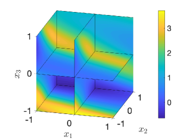
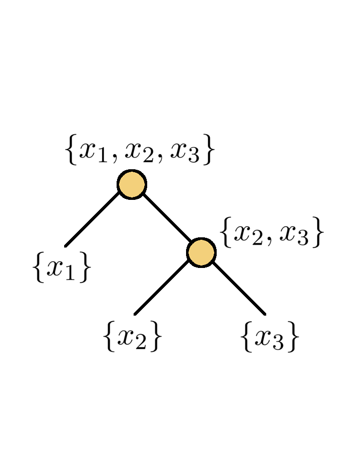
Refer to caption          Refer to caption

Figure 2: Volumetric plot of the three-dimensional function (47) and binary tree representing the tensor format used in the recursive bi-orthogonal decomposition.

We discretize (47) on a three-dimensional tensor product grid with 505050 Gauss-Legendre collocation points [29] in each variable (125000 points total). Regarding the function space in which we perform the decomposition, in this example we set k=0𝑘0k=0 in (2), i.e., we consider the classical L2(Ω)=H0(Ω)superscript𝐿2Ωsuperscript𝐻0ΩL^{2}(\Omega)=H^{0}(\Omega) function space. In this setting, the kernel of the integral operator Lusubscript𝐿𝑢L_{u} in (31) (first level of the binary tree), reduces to

lu(x1,x1)=1111u(x1,x2,x3)u(x1,x2,x3)𝑑x2𝑑x3.subscript𝑙𝑢subscript𝑥1superscriptsubscript𝑥1superscriptsubscript11superscriptsubscript11𝑢subscript𝑥1subscript𝑥2subscript𝑥3𝑢superscriptsubscript𝑥1subscript𝑥2subscript𝑥3differential-dsubscript𝑥2differential-dsubscript𝑥3l_{u}(x_{1},x_{1}^{\prime})=\int_{-1}^{1}\int_{-1}^{1}u(x_{1},x_{2},x_{3})u(x_{1}^{\prime},x_{2},x_{3})dx_{2}dx_{3}. (48)

This integral is computed with the Gauss-Legendre quadrature rule corresponding to the chosen grid points. The x1subscript𝑥1x_{1}-modes are solutions of the eigenvalue problem

11lu(x1,x1)ψi1(1)(x1)𝑑x1=λi12ψi1(1)(x1).superscriptsubscript11subscript𝑙𝑢subscript𝑥1superscriptsubscript𝑥1superscriptsubscript𝜓subscript𝑖11superscriptsubscript𝑥1differential-dsuperscriptsubscript𝑥1superscriptsubscript𝜆subscript𝑖12subscriptsuperscript𝜓1subscript𝑖1subscript𝑥1\int_{-1}^{1}l_{u}(x_{1},x_{1}^{\prime})\psi_{i_{1}}^{(1)}(x_{1}^{\prime})dx_{1}^{\prime}=\lambda_{i_{1}}^{2}\psi^{(1)}_{i_{1}}(x_{1}). (49)

    (a)                                                   (b)                                                   (c)

Refer to caption Refer to caption Refer to caption

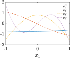
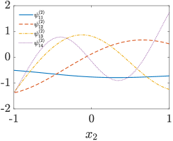
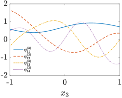
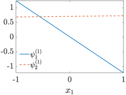
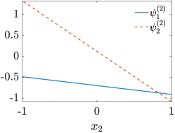
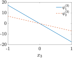
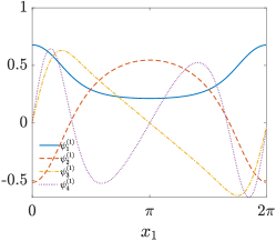
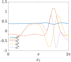
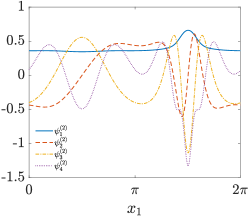
Figure 3: Recursive bi-orthogonal decomposition of the function (47). Shown are a few relevant modes ψi1(1)(x1)subscriptsuperscript𝜓1subscript𝑖1subscript𝑥1\psi^{(1)}_{i_{1}}(x_{1}) (a), ψi1i2(2)(x2)subscriptsuperscript𝜓2subscript𝑖1subscript𝑖2subscript𝑥2\psi^{(2)}_{i_{1}i_{2}}(x_{2}) (b), and ψi1i2(3)(x3)subscriptsuperscript𝜓3subscript𝑖1subscript𝑖2subscript𝑥3\psi^{(3)}_{i_{1}i_{2}}(x_{3}) (c).

        (a)                                                       (b)                                                       (c)

Refer to caption Refer to caption Refer to caption

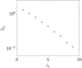
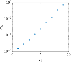
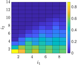
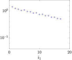
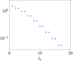
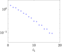
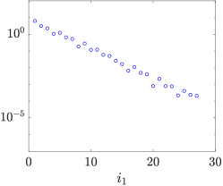
Figure 4: Recursive bi-orthogonal decomposition of the function (47). We plot the level-1 spectrum λi1subscript𝜆subscript𝑖1\lambda_{i_{1}} (a), the level-2 thresholds corresponding to σ=105𝜎superscript105\sigma=10^{-5} (b), and the level-2 spectrum λi1i2subscript𝜆subscript𝑖1subscript𝑖2\lambda_{i_{1}i_{2}} (c).

We discretize (49) using Gauss-Legendre spectral collocation with 50 points. This yields 505050 leading eigenvalues and corresponding eigenfunctions. Following the thresholding technique discussed in Section 2.4, we set σ=105𝜎superscript105\sigma=10^{-5} to determine how many level-1 eigenvalues and eigenfunctions to keep. It turns out that only 999 eigenvalues are larger than σ𝜎\sigma which determines the first truncation rank as r1=9subscript𝑟19r_{1}=9. These 999 eigenvalues {λ1,,λ9}subscript𝜆1subscript𝜆9\{\lambda_{1},\ldots,\lambda_{9}\} constitute the level 111 spectrum which is shown in Figure 4(a). The corresponding eigenfunctions are ψ1(1),,ψ9(1)subscriptsuperscript𝜓11subscriptsuperscript𝜓19\psi^{(1)}_{1},\ldots,\psi^{(1)}_{9}. The modes ψ1(2,3),,ψ9(2,3)subscriptsuperscript𝜓231subscriptsuperscript𝜓239\psi^{(2,3)}_{1},\ldots,\psi^{(2,3)}_{9} can now be obtained through projection as in (32)

ψi1(2,3)=1λi111u(x1,x2,x3)ψi1(1)𝑑x1,subscriptsuperscript𝜓23subscript𝑖11subscript𝜆subscript𝑖1superscriptsubscript11𝑢subscript𝑥1subscript𝑥2subscript𝑥3subscriptsuperscript𝜓1subscript𝑖1differential-dsubscript𝑥1\psi^{(2,3)}_{i_{1}}=\frac{1}{\lambda_{i_{1}}}\int_{-1}^{1}u(x_{1},x_{2},x_{3})\psi^{(1)}_{i_{1}}dx_{1}\ , (50)

which we compute with Gauss-Legendre quadrature. For each of the 999 modes ψi1(2,3)subscriptsuperscript𝜓23subscript𝑖1\psi^{(2,3)}_{i_{1}} we follow the same procedure we used to compute ψi1(1)subscriptsuperscript𝜓1subscript𝑖1\psi^{(1)}_{i_{1}}, i.e., we build the kernels

lψi1(2,3)(x2,x2)=11ψi1(2,3)(x2,x3)ψi1(2,3)(x2,x3)𝑑x3subscript𝑙subscriptsuperscript𝜓23subscript𝑖1subscript𝑥2superscriptsubscript𝑥2superscriptsubscript11superscriptsubscript𝜓subscript𝑖123subscript𝑥2subscript𝑥3superscriptsubscript𝜓subscript𝑖123superscriptsubscript𝑥2subscript𝑥3differential-dsubscript𝑥3l_{\psi^{(2,3)}_{i_{1}}}(x_{2},x_{2}^{\prime})=\int_{-1}^{1}\psi_{i_{1}}^{(2,3)}(x_{2},x_{3})\psi_{i_{1}}^{(2,3)}(x_{2}^{\prime},x_{3})dx_{3} (51)

and then solve the eigenvalue problems

11lψi1(2,3)(x2,x2)ψi1i2(2)(x2)𝑑x2=λi1i22ψi1i2(2)(x2),superscriptsubscript11subscript𝑙subscriptsuperscript𝜓23subscript𝑖1subscript𝑥2superscriptsubscript𝑥2superscriptsubscript𝜓subscript𝑖1subscript𝑖22superscriptsubscript𝑥2differential-dsuperscriptsubscript𝑥2superscriptsubscript𝜆subscript𝑖1subscript𝑖22superscriptsubscript𝜓subscript𝑖1subscript𝑖22subscript𝑥2\int_{-1}^{1}l_{\psi^{(2,3)}_{i_{1}}}(x_{2},x_{2}^{\prime})\psi_{i_{1}i_{2}}^{(2)}(x_{2}^{\prime})dx_{2}^{\prime}=\lambda_{i_{1}i_{2}}^{2}\psi_{i_{1}i_{2}}^{(2)}(x_{2})\ , (52)

to obtain 505050 eigenvalues and eigenfunctions of for each i1=1,,9subscript𝑖119{i_{1}}=1,\ldots,9. To decide how many eigenvalues and eigenfunctions to keep we use the thresholds σi1=σ/λi1subscript𝜎subscript𝑖1𝜎subscript𝜆subscript𝑖1\sigma_{i_{1}}=\sigma/\lambda_{i_{1}} (see Figure 4(b)). This yields the following vector of level-222 ranks r2=[11,11,11,11,11,11,10,6,0]subscript𝑟21111111111111060r_{2}=[11,11,11,11,11,11,10,6,0]. The level-222 spectra λi1i2subscript𝜆subscript𝑖1subscript𝑖2\lambda_{i_{1}i_{2}} is shown in Figure 4(c) for the level-111 modes above the threshold σ=105𝜎superscript105\sigma=10^{-5}.

3 Recursive bi-orthogonal decomposition of time-dependent multivariate functions

Let us consider the time-dependent multivariate function

u:Ω×[0,T].:𝑢Ω0𝑇u:\Omega\times[0,T]\to\mathbb{R}. (53)

At any fixed t[0,T]𝑡0𝑇t\in[0,T] we assume that u(x1,,xd,t)𝑢subscript𝑥1subscript𝑥𝑑𝑡u(x_{1},\dots,x_{d},t) is an element of the Sobolev space (2). With the goal of solving high-dimensional nonlinear evolution equations (PDEs), in this Section we develop a recursive bi-orthogonal decomposition theory for (53). To decompose the function u(x1,,xd,t)𝑢subscript𝑥1subscript𝑥𝑑𝑡u(x_{1},\ldots,x_{d},t) with recursive bi-orthogonal methods we have at least two different options. For instance, if u𝑢u is square integrable in t𝑡t, then we may treat t𝑡t the same as a spatial variable xjsubscript𝑥𝑗x_{j}. In this way, we essentially include the time variable in the inner products (9)-(10), and decompose the time-dependent field (53) using the methods of Section 2.1.

An alternative approach relies on introducing time dependence in all modes appearing in the tensor expansion of u(x1,,xd,t)𝑢subscript𝑥1subscript𝑥𝑑𝑡u(x_{1},\ldots,x_{d},t), and then deriving problem-dependent evolution equations for each mode. To this end, one can enforce, e.g., a dynamic orthogonality (DO) condition or a bi-orthogonality (BO) condition [14, 15, 57, 19, 4] at each level of the binary tree representing the tensor expansion. This generalizes the DO/BO framework originally proposed by Sapsis and Lermusiaux [57], and Cheng et. al. [14], which holds for binary trees with only one level, to binary trees with an arbitrary number of levels. The DO/BO method was originally proposed to solve initial/boundary value problems for nonlinear PDEs with parametric uncertainty modeled by the random vector 𝝃(ω)𝝃𝜔\bm{\xi}(\omega). The key idea was to introduce time-redundancy in a Karhunen-Loève-type expansion of the solution for the purpose of efficiently representing the time evolution of the stochastic modes and the corresponding space-time modes. As we mentioned above, the classical DO/BO expansion corresponds to a binary tree with only one level, where the random field u(𝒙,𝝃,t)𝑢𝒙𝝃𝑡u(\bm{x},\bm{\xi},t) is decomposed as

u(𝒙,𝝃,t)=k=1λk(t)u^k(𝒙,t)Γk(𝝃,t).𝑢𝒙𝝃𝑡superscriptsubscript𝑘1subscript𝜆𝑘𝑡subscript^𝑢𝑘𝒙𝑡subscriptΓ𝑘𝝃𝑡u(\bm{x},\bm{\xi},t)=\sum_{k=1}^{\infty}\lambda_{k}(t)\widehat{u}_{k}(\bm{x},t)\Gamma_{k}(\bm{\xi},t). (54)

In this Section we generalize this idea, and apply it recursively to multivariate functions not necessarily dependent on random parameters, until we obtain an expansion in terms of one-dimensional functions (whenever possible). To illustrate the hierarchical DO/BO method, we consider the TT series expansion (30), and introduce redundant time-dependence in all eigenvalues and eigenmodes. This yields the following representation of (53)

u(x1,,xd,t)=i1=1id1=1λi1(t)λi1id1(t)ψi1(1)(t)ψi1i2(2)(t)ψi1id1(d1)(t)ψi1id1(d)(t).𝑢subscript𝑥1subscript𝑥𝑑𝑡superscriptsubscriptsubscript𝑖11superscriptsubscriptsubscript𝑖𝑑11subscript𝜆subscript𝑖1𝑡subscript𝜆subscript𝑖1subscript𝑖𝑑1𝑡superscriptsubscript𝜓subscript𝑖11𝑡superscriptsubscript𝜓subscript𝑖1subscript𝑖22𝑡superscriptsubscript𝜓subscript𝑖1subscript𝑖𝑑1𝑑1𝑡superscriptsubscript𝜓subscript𝑖1subscript𝑖𝑑1𝑑𝑡u(x_{1},\ldots,x_{d},t)=\sum_{i_{1}=1}^{\infty}\cdots\sum_{i_{d-1}=1}^{\infty}\lambda_{i_{1}}(t)\cdots\lambda_{i_{1}\cdots i_{d-1}}(t)\psi_{i_{1}}^{(1)}(t)\psi_{i_{1}i_{2}}^{(2)}(t)\cdots\psi_{i_{1}\cdots i_{d-1}}^{(d-1)}(t)\psi_{i_{1}\cdots i_{d-1}}^{(d)}(t). (55)

Other tensor expansions corresponding to different binary trees, e.g., the HT expansion sketched in Figure 1, can be generalized in a similar way. Hereafter, we derive the DO and BO evolution equations for the time-dependent modes in (55), and show that these two ways of propagating u(x1,,xd,t)𝑢subscript𝑥1subscript𝑥𝑑𝑡u(x_{1},\ldots,x_{d},t) forward in time on a (smooth) low-dimensional manifold of constant rank [60] are equivalent in the sense that the finite dimensional function spaces containing the DO and BO components are essentially the same.

In the following Sections every function is time dependent, so t𝑡t is omitted from the function arguments. Superscripts indicate spatial dependencies as in Section 2, so spatial arguments of functions are also omitted when there is no ambiguity. Angled brackets ,\langle\cdot,\cdot\rangle here denote the L2=H(0)superscript𝐿2superscript𝐻0L^{2}=H^{(0)} inner product over all spatial components for which the two arguments are defined.

3.1 DO-TT propagator

To derive the Dynamically-Orthogonal Tensor-Train (DO-TT) propagator, let us first consider the level-1 expansion

u(x1,,xd,t)=i1=1r1ψi1(1)(t)Ψi1(2,,d)(t),𝑢subscript𝑥1subscript𝑥𝑑𝑡superscriptsubscriptsubscript𝑖11subscript𝑟1superscriptsubscript𝜓subscript𝑖11𝑡superscriptsubscriptΨsubscript𝑖12𝑑𝑡u(x_{1},\ldots,x_{d},t)=\sum_{i_{1}=1}^{r_{1}}\psi_{i_{1}}^{(1)}(t)\Psi_{i_{1}}^{(2,\ldots,d)}(t)\ , (56)

where

Ψi1(2,,d)(t)=λi1(t)ψi1(2,,d)(t).superscriptsubscriptΨsubscript𝑖12𝑑𝑡subscript𝜆subscript𝑖1𝑡superscriptsubscript𝜓subscript𝑖12𝑑𝑡\Psi_{i_{1}}^{(2,\ldots,d)}(t)=\lambda_{i_{1}}(t)\psi_{i_{1}}^{(2,\ldots,d)}(t). (57)

By differentiating (56) with respect to time we obtain

ut=i1=1r1ψi1(1)tΨi1(2,,d)+ψi1(1)Ψi1(2,,d)t.𝑢𝑡superscriptsubscriptsubscript𝑖11subscript𝑟1superscriptsubscript𝜓subscript𝑖11𝑡superscriptsubscriptΨsubscript𝑖12𝑑superscriptsubscript𝜓subscript𝑖11superscriptsubscriptΨsubscript𝑖12𝑑𝑡\frac{\partial u}{\partial t}=\sum_{i_{1}=1}^{r_{1}}\frac{\partial\psi_{i_{1}}^{(1)}}{\partial t}\Psi_{i_{1}}^{(2,\ldots,d)}+\psi_{i_{1}}^{(1)}\frac{\partial\Psi_{i_{1}}^{(2,\ldots,d)}}{\partial t}. (58)

Clearly, if u(x1,,xd,t)𝑢subscript𝑥1subscript𝑥𝑑𝑡u(x_{1},\ldots,x_{d},t) is given then u/t𝑢𝑡\partial u/\partial t is known, and therefore the left hand side of (58) is fully determined. On the other hand, in the context of nonlinear evolution equations, u/t𝑢𝑡\partial u/\partial t is represented by the right hand side of the PDE. Applying ,ψk1(1)superscriptsubscript𝜓subscript𝑘11\langle\cdot,\psi_{k_{1}}^{(1)}\rangle to (58) and utlizing the DO conditions (see [57])

ψi1(1)t,ψk1(1)=0for alli1,k1=1,2,formulae-sequencesuperscriptsubscript𝜓subscript𝑖11𝑡superscriptsubscript𝜓subscript𝑘110for allsubscript𝑖1subscript𝑘112\displaystyle\langle\frac{\partial\psi_{i_{1}}^{(1)}}{\partial t},\psi_{k_{1}}^{(1)}\rangle=0\qquad\text{for all}\quad i_{1},k_{1}=1,2,\ldots (59)

yields

Ψk1(2,,d)t=ut,ψk1(1)Nk1(2,,d)(t).superscriptsubscriptΨsubscript𝑘12𝑑𝑡subscript𝑢𝑡superscriptsubscript𝜓subscript𝑘11superscriptsubscript𝑁subscript𝑘12𝑑𝑡\frac{\partial\Psi_{k_{1}}^{(2,\ldots,d)}}{\partial t}=\underbrace{\langle\frac{\partial u}{\partial t},\psi_{k_{1}}^{(1)}\rangle}_{N_{k_{1}}^{(2,\ldots,d)}(t)}. (60)

The evolution equations for the modes ψk1(1)superscriptsubscript𝜓subscript𝑘11\psi_{k_{1}}^{(1)} can be obtained by applying ,Ψk1(2,d)superscriptsubscriptΨsubscript𝑘12𝑑\langle\cdot,\Psi_{k_{1}}^{(2,\ldots d)}\rangle to (58) and (60), and the using simple algebra. This yields

i1=1r1ψi1(1)tΨi1(2,,d),Ψk1(2,,d)Ci1k1(t)=ut,Ψk1(2,,d)i1=1r1ψi1(1)ut,Ψk1(2,,d)ψi1(1)Mk1(1)(t).superscriptsubscriptsubscript𝑖11subscript𝑟1superscriptsubscript𝜓subscript𝑖11𝑡subscriptsuperscriptsubscriptΨsubscript𝑖12𝑑superscriptsubscriptΨsubscript𝑘12𝑑subscript𝐶subscript𝑖1subscript𝑘1𝑡subscript𝑢𝑡superscriptsubscriptΨsubscript𝑘12𝑑superscriptsubscriptsubscript𝑖11subscript𝑟1superscriptsubscript𝜓subscript𝑖11𝑢𝑡superscriptsubscriptΨsubscript𝑘12𝑑superscriptsubscript𝜓subscript𝑖11superscriptsubscript𝑀subscript𝑘11𝑡\sum_{i_{1}=1}^{r_{1}}\frac{\partial\psi_{i_{1}}^{(1)}}{\partial t}\underbrace{\langle\Psi_{i_{1}}^{(2,\ldots,d)},\Psi_{k_{1}}^{(2,\ldots,d)}\rangle}_{C_{i_{1}k_{1}}(t)}=\underbrace{\langle\frac{\partial u}{\partial t},\Psi_{k_{1}}^{(2,\ldots,d)}\rangle-\sum_{i_{1}=1}^{r_{1}}\psi_{i_{1}}^{(1)}\langle\frac{\partial u}{\partial t},\Psi_{k_{1}}^{(2,\ldots,d)}\psi_{i_{1}}^{(1)}\rangle}_{M_{k_{1}}^{(1)}(t)}. (61)

Equations (60) and (61) can be conveniently expressed in a matrix-vector form as

𝑪(t)𝝍(1)t=𝑴(1)(t),𝚿(2,,d)t=𝑵(2,,d)(t).formulae-sequence𝑪𝑡superscript𝝍1𝑡superscript𝑴1𝑡superscript𝚿2𝑑𝑡superscript𝑵2𝑑𝑡\displaystyle\bm{C}(t)\frac{\partial\bm{\psi}^{(1)}}{\partial t}=\bm{M}^{(1)}(t),\qquad\frac{\partial\bm{\Psi}^{(2,\ldots,d)}}{\partial t}=\bm{N}^{(2,\ldots,d)}(t). (62)

where

𝝍(1)=[ψ1(1)ψr1(1)],𝚿(2,,d)=[Ψ1(2,,d)Ψr1(2,,d)],formulae-sequencesuperscript𝝍1delimited-[]subscriptsuperscript𝜓11subscriptsuperscript𝜓1subscript𝑟1superscript𝚿2𝑑delimited-[]subscriptsuperscriptΨ2𝑑1subscriptsuperscriptΨ2𝑑subscript𝑟1\bm{\psi}^{(1)}=\left[\begin{array}[]{c}\psi^{(1)}_{1}\\ \vdots\\ \psi^{(1)}_{r_{1}}\end{array}\right],\qquad\bm{\Psi}^{(2,\ldots,d)}=\left[\begin{array}[]{c}\Psi^{(2,\ldots,d)}_{1}\\ \vdots\\ \Psi^{(2,\ldots,d)}_{r_{1}}\end{array}\right], (63)
𝑴(1)(t)=[M1(1)(t)Mr1(1)(t)],𝑵(2,,d)(t)=[N1(2,,d)(t)Nr1(2,,d)(t)].formulae-sequencesuperscript𝑴1𝑡delimited-[]superscriptsubscript𝑀11𝑡superscriptsubscript𝑀subscript𝑟11𝑡superscript𝑵2𝑑𝑡delimited-[]subscriptsuperscript𝑁2𝑑1𝑡subscriptsuperscript𝑁2𝑑subscript𝑟1𝑡\bm{M}^{(1)}(t)=\left[\begin{array}[]{c}M_{1}^{(1)}(t)\\ \vdots\\ M_{r_{1}}^{(1)}(t)\end{array}\right],\qquad\bm{N}^{(2,\ldots,d)}(t)=\left[\begin{array}[]{c}N^{(2,\ldots,d)}_{1}(t)\\ \vdots\\ N^{(2,\ldots,d)}_{r_{1}}(t)\end{array}\right]. (64)

Note that 𝑴(1)(t)superscript𝑴1𝑡\bm{M}^{(1)}(t) and 𝑪(t)𝑪𝑡\bm{C}(t) depend on Ψ(2,,d)superscriptΨ2𝑑\Psi^{(2,\ldots,d)} and u/t𝑢𝑡\partial u/\partial t, while 𝑵(2,,d)(t)superscript𝑵2𝑑𝑡\bm{N}^{(2,\ldots,d)}(t) depends on 𝝍(1)superscript𝝍1\bm{\psi}^{(1)} and u/t𝑢𝑡\partial u/\partial t. Therefore, given u/t𝑢𝑡\partial u/\partial t we have that the system (62) is closed. At this point, we move to the next level of the TT binary tree and derive DO evolution equations for the level-222 modes. By following the same steps as in the derivation of the level-111 system (62), we obtain

Ψk1k2(3,,d)tsuperscriptsubscriptΨsubscript𝑘1subscript𝑘23𝑑𝑡\displaystyle\frac{\partial\Psi_{k_{1}k_{2}}^{(3,\ldots,d)}}{\partial t} =Nk1(2,,d),ψk1k2(2)Nk1k2(3,,d)(t),absentsubscriptsubscriptsuperscript𝑁2𝑑subscript𝑘1superscriptsubscript𝜓subscript𝑘1subscript𝑘22superscriptsubscript𝑁subscript𝑘1subscript𝑘23𝑑𝑡\displaystyle=\underbrace{\langle N^{(2,\ldots,d)}_{k_{1}},\psi_{k_{1}k_{2}}^{(2)}\rangle}_{N_{k_{1}k_{2}}^{(3,\ldots,d)}(t)}\ , (65)
i2=1r2ψk1i2(2)tΨk1i2(3,,d),Ψk1k2(3,,d)superscriptsubscriptsubscript𝑖21subscript𝑟2superscriptsubscript𝜓subscript𝑘1subscript𝑖22𝑡superscriptsubscriptΨsubscript𝑘1subscript𝑖23𝑑superscriptsubscriptΨsubscript𝑘1subscript𝑘23𝑑\displaystyle\sum_{i_{2}=1}^{r_{2}}\frac{\partial\psi_{k_{1}i_{2}}^{(2)}}{\partial t}\langle\Psi_{k_{1}i_{2}}^{(3,\ldots,d)},\Psi_{k_{1}k_{2}}^{(3,\ldots,d)}\rangle =Nk1(2,,d),Ψk1k2(3,,d)i2=1r2ψk1i2(2)Nk1(2,,d),Ψk1k2(3,,d)ψk1i2(2)Mk1k2(2)(t),absentsubscriptsubscriptsuperscript𝑁2𝑑subscript𝑘1superscriptsubscriptΨsubscript𝑘1subscript𝑘23𝑑superscriptsubscriptsubscript𝑖21subscript𝑟2superscriptsubscript𝜓subscript𝑘1subscript𝑖22subscriptsuperscript𝑁2𝑑subscript𝑘1superscriptsubscriptΨsubscript𝑘1subscript𝑘23𝑑superscriptsubscript𝜓subscript𝑘1subscript𝑖22superscriptsubscript𝑀subscript𝑘1subscript𝑘22𝑡\displaystyle=\underbrace{\langle N^{(2,\ldots,d)}_{k_{1}},\Psi_{k_{1}k_{2}}^{(3,\ldots,d)}\rangle-\sum_{i_{2}=1}^{r_{2}}\psi_{k_{1}i_{2}}^{(2)}\langle N^{(2,\ldots,d)}_{k_{1}},\Psi_{k_{1}k_{2}}^{(3,\ldots,d)}\psi_{k_{1}i_{2}}^{(2)}\rangle}_{M_{k_{1}k_{2}}^{(2)}(t)}\ ,

where we defined

Ψk1k2(3,,d)=λk1k2(t)ψk1k2(3,,d)(t).superscriptsubscriptΨsubscript𝑘1subscript𝑘23𝑑subscript𝜆subscript𝑘1subscript𝑘2𝑡superscriptsubscript𝜓subscript𝑘1subscript𝑘23𝑑𝑡\Psi_{k_{1}k_{2}}^{(3,\ldots,d)}=\lambda_{k_{1}k_{2}}(t)\psi_{k_{1}k_{2}}^{(3,\ldots,d)}(t). (66)

Proceeding recursively, it is possible to obtain evolution equations for each mode in the TT binary tree sketched in Figure 1. Specifically, we have

Ψk1kj(j+1,,d)t=superscriptsubscriptΨsubscript𝑘1subscript𝑘𝑗𝑗1𝑑𝑡absent\displaystyle\frac{\partial\Psi_{k_{1}\cdots k_{j}}^{(j+1,\ldots,d)}}{\partial t}= Nk1kj1(j,,d),ψk1kj(j)Nk1kj(j+1,,d)(t)subscriptsubscriptsuperscript𝑁𝑗𝑑subscript𝑘1subscript𝑘𝑗1superscriptsubscript𝜓subscript𝑘1subscript𝑘𝑗𝑗superscriptsubscript𝑁subscript𝑘1subscript𝑘𝑗𝑗1𝑑𝑡\displaystyle\underbrace{\langle N^{(j,\ldots,d)}_{k_{1}\cdots k_{j-1}},\psi_{k_{1}\cdots k_{j}}^{(j)}\rangle}_{N_{k_{1}\cdots k_{j}}^{(j+1,\ldots,d)}(t)} (67)
ij=1rjψk1kj1ij(j)tsuperscriptsubscriptsubscript𝑖𝑗1subscript𝑟𝑗subscriptsuperscript𝜓𝑗subscript𝑘1subscript𝑘𝑗1subscript𝑖𝑗𝑡\displaystyle\sum_{i_{j}=1}^{r_{j}}\frac{\partial\psi^{(j)}_{k_{1}\cdots k_{j-1}i_{j}}}{\partial t} Ψk1kj1ij(j+1,,d),Ψk1kj(j+1,,d)superscriptsubscriptΨsubscript𝑘1subscript𝑘𝑗1subscript𝑖𝑗𝑗1𝑑superscriptsubscriptΨsubscript𝑘1subscript𝑘𝑗𝑗1𝑑\displaystyle\langle\Psi_{k_{1}\cdots k_{j-1}i_{j}}^{(j+1,\ldots,d)},\Psi_{k_{1}\cdots k_{j}}^{(j+1,\ldots,d)}\rangle (68)
=Nk1kj1,Ψk1kj(j+1,,d)ij=1rjψk1kj1ijNk1kj1(j,,d),Ψk1kj(j+1,,d)ψk1kj1ij(j)Mk1kj(j)(t).absentsubscriptsubscript𝑁subscript𝑘1subscript𝑘𝑗1superscriptsubscriptΨsubscript𝑘1subscript𝑘𝑗𝑗1𝑑superscriptsubscriptsubscript𝑖𝑗1subscript𝑟𝑗subscript𝜓subscript𝑘1subscript𝑘𝑗1subscript𝑖𝑗subscriptsuperscript𝑁𝑗𝑑subscript𝑘1subscript𝑘𝑗1superscriptsubscriptΨsubscript𝑘1subscript𝑘𝑗𝑗1𝑑superscriptsubscript𝜓subscript𝑘1subscript𝑘𝑗1subscript𝑖𝑗𝑗superscriptsubscript𝑀subscript𝑘1subscript𝑘𝑗𝑗𝑡\displaystyle=\underbrace{\langle N_{k_{1}\cdots k_{j-1}},\Psi_{k_{1}\cdots k_{j}}^{(j+1,\ldots,d)}\rangle-\sum_{i_{j}=1}^{r_{j}}\psi_{k_{1}\cdots k_{j-1}i_{j}}\langle N^{(j,\ldots,d)}_{k_{1}\cdots k_{j-1}},\Psi_{k_{1}\cdots k_{j}}^{(j+1,\ldots,d)}\psi_{k_{1}\cdots k_{j-1}i_{j}}^{(j)}\rangle}_{M_{k_{1}\cdots k_{j}}^{(j)}(t)}. (69)

Equations (68)-(69) can be conveniently expressed in a matrix-vector form as

𝑪i1ij1(t)𝝍i1ij1(j)t=𝑴i1ij1(j)(t),𝚿i1ij(j+1,,d)t=𝑵k1kj(j+1,,d)(t).formulae-sequencesubscript𝑪subscript𝑖1subscript𝑖𝑗1𝑡superscriptsubscript𝝍subscript𝑖1subscript𝑖𝑗1𝑗𝑡subscriptsuperscript𝑴𝑗subscript𝑖1subscript𝑖𝑗1𝑡subscriptsuperscript𝚿𝑗1𝑑subscript𝑖1subscript𝑖𝑗𝑡subscriptsuperscript𝑵𝑗1𝑑subscript𝑘1subscript𝑘𝑗𝑡\displaystyle\bm{C}_{i_{1}\cdots i_{j-1}}(t)\frac{\partial\bm{\psi}_{i_{1}\cdots i_{j-1}}^{(j)}}{\partial t}=\bm{M}^{(j)}_{i_{1}\cdots i_{j-1}}(t),\qquad\frac{\partial\bm{\Psi}^{(j+1,\ldots,d)}_{i_{1}\cdots i_{j}}}{\partial t}=\bm{N}^{(j+1,\ldots,d)}_{k_{1}\cdots k_{j}}(t). (70)

where,

𝝍i1ij1(j)=[ψi1ij11(j)ψi1ij1rj(j)],𝚿i1ij(j+1,,d)=[Ψi1ij1(j+1,,d)Ψi1ijrj(j+1,,d)],formulae-sequencesuperscriptsubscript𝝍subscript𝑖1subscript𝑖𝑗1𝑗delimited-[]superscriptsubscript𝜓subscript𝑖1subscript𝑖𝑗11𝑗superscriptsubscript𝜓subscript𝑖1subscript𝑖𝑗1subscript𝑟𝑗𝑗subscriptsuperscript𝚿𝑗1𝑑subscript𝑖1subscript𝑖𝑗delimited-[]subscriptsuperscriptΨ𝑗1𝑑subscript𝑖1subscript𝑖𝑗1subscriptsuperscriptΨ𝑗1𝑑subscript𝑖1subscript𝑖𝑗subscript𝑟𝑗\bm{\psi}_{i_{1}\cdots i_{j-1}}^{(j)}=\left[\begin{array}[]{c}\psi_{i_{1}\cdots i_{j-1}1}^{(j)}\\ \vdots\\ \psi_{i_{1}\cdots i_{j-1}r_{j}}^{(j)}\end{array}\right],\qquad\bm{\Psi}^{(j+1,\ldots,d)}_{i_{1}\cdots i_{j}}=\left[\begin{array}[]{c}\Psi^{(j+1,\ldots,d)}_{i_{1}\cdots i_{j}1}\\ \vdots\\ \Psi^{(j+1,\ldots,d)}_{i_{1}\cdots i_{j}r_{j}}\end{array}\right], (71)
𝑴i1ij1(j)(t)=[Mi1ij11(j)(t)Mi1ij1rj(j)(t)],𝑵k1kj(j+1,,d)(t)=[Nk1kj1(j+1,,d)(t)Nk1kjrj(j+1,,d)(t)].formulae-sequencesubscriptsuperscript𝑴𝑗subscript𝑖1subscript𝑖𝑗1𝑡delimited-[]subscriptsuperscript𝑀𝑗subscript𝑖1subscript𝑖𝑗11𝑡subscriptsuperscript𝑀𝑗subscript𝑖1subscript𝑖𝑗1subscript𝑟𝑗𝑡subscriptsuperscript𝑵𝑗1𝑑subscript𝑘1subscript𝑘𝑗𝑡delimited-[]subscriptsuperscript𝑁𝑗1𝑑subscript𝑘1subscript𝑘𝑗1𝑡subscriptsuperscript𝑁𝑗1𝑑subscript𝑘1subscript𝑘𝑗subscript𝑟𝑗𝑡\bm{M}^{(j)}_{i_{1}\cdots i_{j-1}}(t)=\left[\begin{array}[]{c}M^{(j)}_{i_{1}\cdots i_{j-1}1}(t)\\ \vdots\\ M^{(j)}_{i_{1}\cdots i_{j-1}r_{j}}(t)\end{array}\right],\qquad\bm{N}^{(j+1,\ldots,d)}_{k_{1}\cdots k_{j}}(t)=\left[\begin{array}[]{c}N^{(j+1,\ldots,d)}_{k_{1}\cdots k_{j}1}(t)\\ \vdots\\ N^{(j+1,\ldots,d)}_{k_{1}\cdots k_{j}r_{j}}(t)\end{array}\right]. (72)
Remark

The “non-leaf” modes ψk1kj(j+1,,d)superscriptsubscript𝜓subscript𝑘1subscript𝑘𝑗𝑗1𝑑\psi_{k_{1}\cdots k_{j}}^{(j+1,\ldots,d)} can be constructed at any time in terms of the “leaf” modes as

ψk1kj(j+1,,d)=ij+1=1rj+1id1=1rd1ψk1kjij+1(j+1)ψk1kjij+1id1(d1)ψk1kjij+1id1(d)superscriptsubscript𝜓subscript𝑘1subscript𝑘𝑗𝑗1𝑑superscriptsubscriptsubscript𝑖𝑗11subscript𝑟𝑗1superscriptsubscriptsubscript𝑖𝑑11subscript𝑟𝑑1superscriptsubscript𝜓subscript𝑘1subscript𝑘𝑗subscript𝑖𝑗1𝑗1superscriptsubscript𝜓subscript𝑘1subscript𝑘𝑗subscript𝑖𝑗1subscript𝑖𝑑1𝑑1superscriptsubscript𝜓subscript𝑘1subscript𝑘𝑗subscript𝑖𝑗1subscript𝑖𝑑1𝑑\psi_{k_{1}\cdots k_{j}}^{(j+1,\ldots,d)}=\sum_{i_{j+1}=1}^{r_{j+1}}\cdots\sum_{i_{d-1}=1}^{r_{d-1}}\psi_{k_{1}\cdots k_{j}i_{j+1}}^{(j+1)}\cdots\psi_{k_{1}\cdots k_{j}i_{j+1}\cdots i_{d-1}}^{(d-1)}\psi_{k_{1}\cdots k_{j}i_{j+1}\cdots i_{d-1}}^{(d)} (73)

To build the time-dependent multivariate function (55) it is sufficient to integrate only the evolution equations corresponding to the leaf modes.

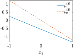
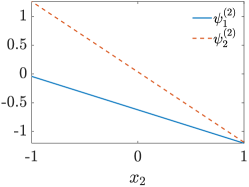
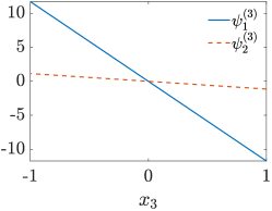
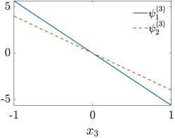
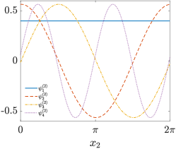
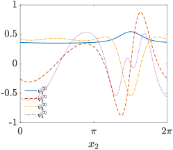
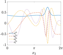
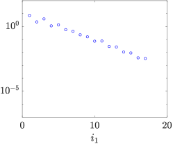
3.2 An example: DO-TT decomposition of a time-dependent 3D function

Let us consider the time-dependent multivariate function

u(x1,x2,x3,t)=(t+1)x2x3+(t210)x1x3(4sin(t)+3)x1x2x3,(x1,x2,x3)Ω.formulae-sequence𝑢subscript𝑥1subscript𝑥2subscript𝑥3𝑡𝑡1subscript𝑥2subscript𝑥3superscript𝑡210subscript𝑥1subscript𝑥34𝑡3subscript𝑥1subscript𝑥2subscript𝑥3subscript𝑥1subscript𝑥2subscript𝑥3Ωu(x_{1},x_{2},x_{3},t)=(t+1)x_{2}x_{3}+(t^{2}-10)x_{1}x_{3}-(4\sin(t)+3)x_{1}x_{2}x_{3},\qquad(x_{1},x_{2},x_{3})\in\Omega. (74)

where Ω=[1,1]3Ωsuperscript113\Omega=[-1,1]^{3} is the standard three-dimensional cube. We are interested in decomposing (74) with the DO-TT method. To this end, we consider the L2superscript𝐿2L^{2} inner product and first perform a recursive bi-orthogonal decomposition of the initial state u(x1,x2,x3,0)𝑢subscript𝑥1subscript𝑥2subscript𝑥30u(x_{1},x_{2},x_{3},0) using the methods of Section 2.1. To this end, we consider 505050 Gauss-Legendre quadrature points and set the eigenvalue threshold to σ=105𝜎superscript105\sigma=10^{-5}. By following the same steps as in the example 2.4.1, this yields multivariate ranks r1=2subscript𝑟12r_{1}=2 and r2=[1 1]subscript𝑟2delimited-[]11r_{2}=[1\,1]. This allows us to approximate the initial condition as

u(x1,x2,x3,0)ψ1(1)(0)ψ11(2)(0)ψ11(3)(0)+ψ2(1)(0)ψ21(2)(0)ψ21(3)(0).similar-to-or-equals𝑢subscript𝑥1subscript𝑥2subscript𝑥30subscriptsuperscript𝜓110subscriptsuperscript𝜓2110subscriptsuperscript𝜓3110subscriptsuperscript𝜓120subscriptsuperscript𝜓2210subscriptsuperscript𝜓3210u(x_{1},x_{2},x_{3},0)\simeq\psi^{(1)}_{1}(0)\psi^{(2)}_{11}(0)\psi^{(3)}_{11}(0)+\psi^{(1)}_{2}(0)\psi^{(2)}_{21}(0)\psi^{(3)}_{21}(0). (75)

The time derivative of u𝑢u is easily obtained as

ut=x2x3+2tx1x34cos(t)x1x2x3.𝑢𝑡subscript𝑥2subscript𝑥32𝑡subscript𝑥1subscript𝑥34𝑡subscript𝑥1subscript𝑥2subscript𝑥3\frac{\partial u}{\partial t}=x_{2}x_{3}+2tx_{1}x_{3}-4\cos(t)x_{1}x_{2}x_{3}. (76)

A substitution of (76) intro the multi-level DO evolution equations (70) yields

ψk(1)t=subscriptsuperscript𝜓1𝑘𝑡absent\displaystyle\frac{\partial\psi^{(1)}_{k}}{\partial t}= x2x3ψk(2,3)+2tx1x3ψk(2,3)4cos(t)x1x2x3ψk(2,3)delimited-⟨⟩subscript𝑥2subscript𝑥3subscriptsuperscript𝜓23𝑘2𝑡subscript𝑥1delimited-⟨⟩subscript𝑥3superscriptsubscript𝜓𝑘234𝑡subscript𝑥1delimited-⟨⟩subscript𝑥2subscript𝑥3subscriptsuperscript𝜓23𝑘\displaystyle\langle x_{2}x_{3}\psi^{(2,3)}_{k}\rangle+2tx_{1}\langle x_{3}\psi_{k}^{(2,3)}\rangle-4\cos(t)x_{1}\langle x_{2}x_{3}\psi^{(2,3)}_{k}\rangle
i=1r1ψi(1)[ψi(1)x2x3ψk(2,3)+2tx1ψi(1)x3ψk(2,3)\displaystyle-\sum_{i=1}^{r_{1}}\psi_{i}^{(1)}\left[\langle\psi^{(1)}_{i}\rangle\langle x_{2}x_{3}\psi^{(2,3)}_{k}\rangle+2t\langle x_{1}\psi^{(1)}_{i}\rangle\langle x_{3}\psi^{(2,3)}_{k}\rangle-\right.
4cos(t)x1ψi(1)x2x3ψk(2,3)],\displaystyle\left.4\cos(t)\langle x_{1}\psi^{(1)}_{i}\rangle\langle x_{2}x_{3}\psi^{(2,3)}_{k}\rangle\right]\ , (77)
ψk1(2)tψk1(3)ψk1(3)=subscriptsuperscript𝜓2𝑘1𝑡delimited-⟨⟩subscriptsuperscript𝜓3𝑘1subscriptsuperscript𝜓3𝑘1absent\displaystyle\frac{\partial\psi^{(2)}_{k1}}{\partial t}\langle\psi^{(3)}_{k1}\psi^{(3)}_{k1}\rangle= x2x3ψk1(3)ψk(1)+2tx3ψk1(3)x1ψk(1)4cos(t)x2x3ψk1(3)x1ψk(1)subscript𝑥2delimited-⟨⟩subscript𝑥3subscriptsuperscript𝜓3𝑘1delimited-⟨⟩subscriptsuperscript𝜓1𝑘2𝑡delimited-⟨⟩subscript𝑥3subscriptsuperscript𝜓3𝑘1delimited-⟨⟩subscript𝑥1subscriptsuperscript𝜓1𝑘4𝑡subscript𝑥2delimited-⟨⟩subscript𝑥3subscriptsuperscript𝜓3𝑘1delimited-⟨⟩subscript𝑥1subscriptsuperscript𝜓1𝑘\displaystyle x_{2}\langle x_{3}\psi^{(3)}_{k1}\rangle\langle\psi^{(1)}_{k}\rangle+2t\langle x_{3}\psi^{(3)}_{k1}\rangle\langle x_{1}\psi^{(1)}_{k}\rangle-4\cos(t)x_{2}\langle x_{3}\psi^{(3)}_{k1}\rangle\langle x_{1}\psi^{(1)}_{k}\rangle
ψk1(2)[x2ψk1(2)x3ψk1(3)ψk(1)+2tψk1(2)x3ψk1(3)x1ψk(1)\displaystyle-\psi^{(2)}_{k1}\left[\langle x_{2}\psi^{(2)}_{k1}\rangle\langle x_{3}\psi^{(3)}_{k1}\rangle\langle\psi^{(1)}_{k}\rangle+2t\langle\psi^{(2)}_{k1}\rangle\langle x_{3}\psi^{(3)}_{k1}\rangle\langle x_{1}\psi^{(1)}_{k}\rangle\right.
4cos(t)x2ψk1(2)x3ψk1(3)x1ψk(1)],\displaystyle\left.-4\cos(t)\langle x_{2}\psi^{(2)}_{k1}\rangle\langle x_{3}\psi^{(3)}_{k1}\rangle\langle x_{1}\psi^{(1)}_{k}\rangle\right]\ , (78)
ψk1(3)t=subscriptsuperscript𝜓3𝑘1𝑡absent\displaystyle\frac{\partial\psi^{(3)}_{k1}}{\partial t}= x3x2ψk1(2)ψk(1)+2tx3ψk1(2)x1ψk(1)4cos(t)x3x2ψk1(2)x1ψk(1),subscript𝑥3delimited-⟨⟩subscript𝑥2subscriptsuperscript𝜓2𝑘1delimited-⟨⟩subscriptsuperscript𝜓1𝑘2𝑡subscript𝑥3delimited-⟨⟩subscriptsuperscript𝜓2𝑘1delimited-⟨⟩subscript𝑥1subscriptsuperscript𝜓1𝑘4𝑡subscript𝑥3delimited-⟨⟩subscript𝑥2subscriptsuperscript𝜓2𝑘1delimited-⟨⟩subscript𝑥1subscriptsuperscript𝜓1𝑘\displaystyle x_{3}\langle x_{2}\psi^{(2)}_{k1}\rangle\langle\psi^{(1)}_{k}\rangle+2tx_{3}\langle\psi^{(2)}_{k1}\rangle\langle x_{1}\psi^{(1)}_{k}\rangle-4\cos(t)x_{3}\langle x_{2}\psi^{(2)}_{k1}\rangle\langle x_{1}\psi^{(1)}_{k}\rangle\ , (79)

for j=1,2𝑗12j=1,2. In a spectral collocation setting, all modes are represented by their values at the 50 Gauss-Legendre collocation points. Hence, the DO evolution equations reduce to a system of ODEs. All integrals in (77)-(79) are computed by using the one-dimensional Gauss-Legendre quadrature rule. In Figure 5 we plot the temporal evolution of all 666 modes appearing in the system (77)-(79). The time-dependent L2(Ω)superscript𝐿2ΩL^{2}(\Omega) error between the DO-TT expansion

u(t,x1,x2,x3)=ψ1(1)(t)ψ11(2)(t)ψ11(3)(t)+ψ2(1)(t)ψ21(2)(t)ψ21(3)(t),𝑢𝑡subscript𝑥1subscript𝑥2subscript𝑥3subscriptsuperscript𝜓11𝑡subscriptsuperscript𝜓211𝑡subscriptsuperscript𝜓311𝑡subscriptsuperscript𝜓12𝑡subscriptsuperscript𝜓221𝑡subscriptsuperscript𝜓321𝑡u(t,x_{1},x_{2},x_{3})=\psi^{(1)}_{1}(t)\psi^{(2)}_{11}(t)\psi^{(3)}_{11}(t)+\psi^{(1)}_{2}(t)\psi^{(2)}_{21}(t)\psi^{(3)}_{21}(t), (80)

and the function (74) is plotted in Figure 6 versus time. We notice that (74) is a separable function with rank r1=2subscript𝑟12r_{1}=2, r2=[1,1]subscript𝑟211r_{2}=[1,1] at each time t𝑡t. This means that it can be represented exactly on a low-dimensional tensor manifold of constant rank at each time. This is the reason why the L2superscript𝐿2L^{2} error in Figure 6 is of order 108superscript10810^{-8} for all t0𝑡0t\geq 0. In general, the multivariate function u(x1,,xd,t)𝑢subscript𝑥1subscript𝑥𝑑𝑡u(x_{1},\ldots,x_{d},t) is not separable and may become rougher/wavier as time increases. In these cases, the multivariate rank (r1,,rd1)subscript𝑟1subscript𝑟𝑑1(r_{1},\ldots,r_{d-1}) of the DO-TT expansion usually needs to be increased in time to accurately represent represent u(x1,,xd,t)𝑢subscript𝑥1subscript𝑥𝑑𝑡u(x_{1},\ldots,x_{d},t). Methods for increasing rank will be addressed in Section 4.1 in the context of adaptive DO-TT approximation of the solution to high-dimensional PDEs.

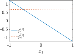
     t=0.0𝑡0.0t=0.0                                             t=2.5𝑡2.5t=2.5                                             t=5.0𝑡5.0t=5.0

Refer to caption Refer to caption Refer to caption

Refer to caption Refer to caption Refer to caption

Refer to caption Refer to caption Refer to caption

Figure 5: Temporal evolution of the bi-orthogonal modes in the DO-TT expansion (80).

Refer to caption

Figure 6: Time-dependent L2(Ω)superscript𝐿2ΩL^{2}(\Omega) error between of the DD-TT expansion (80) and the multivariate function (74).

.

3.3 BO-TT propagator

Alongside the multi-level DO propagator (70), we derive the Bi-Orthogonal Tensor-Train (BO-TT) propagator. The key idea is to replace the dynamic orthogonality condition between the modes at each level of the binary tree, with a bi-orthogonality condition (see [14]). To this end, let us consider the following sequence of bi-orthogonal decompositions

u(x1,,xd,t)=𝑢subscript𝑥1subscript𝑥𝑑𝑡absent\displaystyle u(x_{1},\ldots,x_{d},t)= i1=1φi1(1)(t)φi1(2,,d)(t)superscriptsubscriptsubscript𝑖11superscriptsubscript𝜑subscript𝑖11𝑡superscriptsubscript𝜑subscript𝑖12𝑑𝑡\displaystyle\sum_{i_{1}=1}^{\infty}\varphi_{i_{1}}^{(1)}(t)\varphi_{i_{1}}^{(2,\ldots,d)}(t)
=\displaystyle= i1=1i2=1φi1(1)(t)φi1i2(2)(t)φi1i2(3,,d)(t),superscriptsubscriptsubscript𝑖11superscriptsubscriptsubscript𝑖21superscriptsubscript𝜑subscript𝑖11𝑡superscriptsubscript𝜑subscript𝑖1subscript𝑖22𝑡superscriptsubscript𝜑subscript𝑖1subscript𝑖23𝑑𝑡\displaystyle\sum_{i_{1}=1}^{\infty}\sum_{i_{2}=1}^{\infty}\varphi_{i_{1}}^{(1)}(t)\varphi_{i_{1}i_{2}}^{(2)}(t)\varphi_{i_{1}i_{2}}^{(3,\ldots,d)}(t),
=\displaystyle= i1=1i2=1i3=1φi1(1)(t)φi1i2(2)(t)φi1i2i3(3)(t)φi1i2i3(4,,d)(t)superscriptsubscriptsubscript𝑖11superscriptsubscriptsubscript𝑖21superscriptsubscriptsubscript𝑖31superscriptsubscript𝜑subscript𝑖11𝑡superscriptsubscript𝜑subscript𝑖1subscript𝑖22𝑡superscriptsubscript𝜑subscript𝑖1subscript𝑖2subscript𝑖33𝑡superscriptsubscript𝜑subscript𝑖1subscript𝑖2subscript𝑖34𝑑𝑡\displaystyle\sum_{i_{1}=1}^{\infty}\sum_{i_{2}=1}^{\infty}\sum_{i_{3}=1}^{\infty}\varphi_{i_{1}}^{(1)}(t)\varphi_{i_{1}i_{2}}^{(2)}(t)\varphi_{i_{1}i_{2}i_{3}}^{(3)}(t)\varphi_{i_{1}i_{2}i_{3}}^{(4,\ldots,d)}(t) (81)
\displaystyle\cdots

where the modes φi1ij1k(j)(t)superscriptsubscript𝜑subscript𝑖1subscript𝑖𝑗1𝑘𝑗𝑡\varphi_{i_{1}\cdots i_{j-1}k}^{(j)}(t) and φi1ij1k(j+1,,d)(t)superscriptsubscript𝜑subscript𝑖1subscript𝑖𝑗1𝑘𝑗1𝑑𝑡\varphi_{i_{1}\cdots i_{j-1}k}^{(j+1,\ldots,d)}(t) satisfy the orthogonality conditions

φi1ij1k(j)(t),φi1ij1p(j)(t)superscriptsubscript𝜑subscript𝑖1subscript𝑖𝑗1𝑘𝑗𝑡superscriptsubscript𝜑subscript𝑖1subscript𝑖𝑗1𝑝𝑗𝑡\displaystyle\langle\varphi_{i_{1}\dots i_{j-1}k}^{(j)}(t),\varphi_{i_{1}\dots i_{j-1}p}^{(j)}(t)\rangle =λk(t)δkp,absentsubscript𝜆𝑘𝑡subscript𝛿𝑘𝑝\displaystyle=\lambda_{k}(t)\delta_{kp}, (82)
φi1ij1k(j+1,,d)(t),φi1ij1p(j+1,,d)(t)superscriptsubscript𝜑subscript𝑖1subscript𝑖𝑗1𝑘𝑗1𝑑𝑡superscriptsubscript𝜑subscript𝑖1subscript𝑖𝑗1𝑝𝑗1𝑑𝑡\displaystyle\langle\varphi_{i_{1}\dots i_{j-1}k}^{(j+1,\ldots,d)}(t),\varphi_{i_{1}\dots i_{j-1}p}^{(j+1,\ldots,d)}(t)\rangle =δkp,absentsubscript𝛿𝑘𝑝\displaystyle=\delta_{kp}, (83)

for all t0𝑡0t\geq 0. In contrast with the multi-level DO modes, here the one-dimensional BO modes carry the eigenvalues. By extending the derivation given in [14, 15] to the case of multi-level binary trees, it is straightforward to obtain the following BO-TT evolution equations

𝝋i1ij1(j)t=𝑴i1ij1(t)𝝋i1ij1(j)+𝒑i1ij1(j)(t),subscriptsuperscript𝝋𝑗subscript𝑖1subscript𝑖𝑗1𝑡subscript𝑴subscript𝑖1subscript𝑖𝑗1𝑡subscriptsuperscript𝝋𝑗subscript𝑖1subscript𝑖𝑗1subscriptsuperscript𝒑𝑗subscript𝑖1subscript𝑖𝑗1𝑡\displaystyle\frac{\partial\bm{\varphi}^{(j)}_{i_{1}\cdots i_{j-1}}}{\partial t}=\bm{M}_{i_{1}\cdots i_{j-1}}(t)\bm{\varphi}^{(j)}_{i_{1}\cdots i_{j-1}}+\bm{p}^{(j)}_{i_{1}\cdots i_{j-1}}(t)\ , (84)
𝚲i1ij1(t)𝝋i1ij1(j+1,,d)t=𝑺i1ij1(t)𝝋i1ij1(j+1,,d)+𝒉i1ij1(j+1,,d)(t),subscript𝚲subscript𝑖1subscript𝑖𝑗1𝑡superscriptsubscript𝝋subscript𝑖1subscript𝑖𝑗1𝑗1𝑑𝑡subscript𝑺subscript𝑖1subscript𝑖𝑗1𝑡superscriptsubscript𝝋subscript𝑖1subscript𝑖𝑗1𝑗1𝑑subscriptsuperscript𝒉𝑗1𝑑subscript𝑖1subscript𝑖𝑗1𝑡\displaystyle\bm{\Lambda}_{i_{1}\cdots i_{j-1}}(t)\frac{\partial\bm{\varphi}_{i_{1}\cdots i_{j-1}}^{(j+1,\ldots,d)}}{\partial t}=-\bm{S}_{i_{1}\cdots i_{j-1}}(t)\bm{\varphi}_{i_{1}\cdots i_{j-1}}^{(j+1,\ldots,d)}+\bm{h}^{(j+1,\ldots,d)}_{i_{1}\cdots i_{j-1}}(t)\ ,

where

𝝋i1ij1(j)=[φi1ij11(j)φi1ij1rj(j)],𝝋i1ij1(j+1,d)=[φi1ij11(j+1,d)φi1ij1rj(j+1,d)],formulae-sequencesuperscriptsubscript𝝋subscript𝑖1subscript𝑖𝑗1𝑗delimited-[]superscriptsubscript𝜑subscript𝑖1subscript𝑖𝑗11𝑗superscriptsubscript𝜑subscript𝑖1subscript𝑖𝑗1subscript𝑟𝑗𝑗superscriptsubscript𝝋subscript𝑖1subscript𝑖𝑗1𝑗1𝑑delimited-[]superscriptsubscript𝜑subscript𝑖1subscript𝑖𝑗11𝑗1𝑑superscriptsubscript𝜑subscript𝑖1subscript𝑖𝑗1subscript𝑟𝑗𝑗1𝑑\bm{\varphi}_{i_{1}\cdots i_{j-1}}^{(j)}=\left[\begin{array}[]{c}\varphi_{i_{1}\cdots i_{j-1}1}^{(j)}\\ \vdots\\ \varphi_{i_{1}\cdots i_{j-1}r_{j}}^{(j)}\end{array}\right]\ ,\qquad\bm{\varphi}_{i_{1}\cdots i_{j-1}}^{(j+1,\ldots d)}=\left[\begin{array}[]{c}\varphi_{i_{1}\cdots i_{j-1}1}^{(j+1,\ldots d)}\\ \vdots\\ \varphi_{i_{1}\cdots i_{j-1}r_{j}}^{(j+1,\ldots d)}\end{array}\right]\ , (85)

and

𝒉i1ij1(j+1,,d)=Ni1ij1(j,,d),𝝋i1ij1(j),𝒑i1ij1(j)=Ni1ij1(j,,d),𝝋i1ij1(j+1,,d),formulae-sequencesubscriptsuperscript𝒉𝑗1𝑑subscript𝑖1subscript𝑖𝑗1superscriptsubscript𝑁subscript𝑖1subscript𝑖𝑗1𝑗𝑑subscriptsuperscript𝝋𝑗subscript𝑖1subscript𝑖𝑗1subscriptsuperscript𝒑𝑗subscript𝑖1subscript𝑖𝑗1superscriptsubscript𝑁subscript𝑖1subscript𝑖𝑗1𝑗𝑑subscriptsuperscript𝝋𝑗1𝑑subscript𝑖1subscript𝑖𝑗1\bm{h}^{(j+1,\ldots,d)}_{i_{1}\cdots i_{j-1}}=\langle N_{i_{1}\cdots i_{j-1}}^{(j,\ldots,d)},\bm{\varphi}^{(j)}_{i_{1}\cdots i_{j-1}}\rangle\ ,\qquad\bm{p}^{(j)}_{i_{1}\cdots i_{j-1}}=\langle N_{i_{1}\cdots i_{j-1}}^{(j,\ldots,d)},\bm{\varphi}^{(j+1,\ldots,d)}_{i_{1}\cdots i_{j-1}}\rangle\ , (86)
𝚲i1ij1(t)=𝝋i1ij1(j),𝝋i1ij1(j),𝑴i1ij1(t)=𝝋i1ij1(j+1,,d),𝝋i1ij1(j+1,,d)t,formulae-sequencesubscript𝚲subscript𝑖1subscript𝑖𝑗1𝑡superscriptsubscript𝝋subscript𝑖1subscript𝑖𝑗1𝑗superscriptsubscript𝝋subscript𝑖1subscript𝑖𝑗1𝑗subscript𝑴subscript𝑖1subscript𝑖𝑗1𝑡superscriptsubscript𝝋subscript𝑖1subscript𝑖𝑗1𝑗1𝑑superscriptsubscript𝝋subscript𝑖1subscript𝑖𝑗1𝑗1𝑑𝑡\bm{\Lambda}_{i_{1}\cdots i_{j-1}}(t)=\langle\bm{\varphi}_{i_{1}\cdots i_{j-1}}^{(j)},\bm{\varphi}_{i_{1}\cdots i_{j-1}}^{(j)}\rangle\ ,\qquad\bm{M}_{i_{1}\cdots i_{j-1}}(t)=\langle\bm{\varphi}_{i_{1}\cdots i_{j-1}}^{(j+1,\ldots,d)},\frac{\partial\bm{\varphi}_{i_{1}\cdots i_{j-1}}^{(j+1,\ldots,d)}}{\partial t}\rangle\ , (87)
𝑺i1ij1(t)=𝝋i1ij1(j),𝝋i1ij1(j)t,subscript𝑺subscript𝑖1subscript𝑖𝑗1𝑡superscriptsubscript𝝋subscript𝑖1subscript𝑖𝑗1𝑗superscriptsubscript𝝋subscript𝑖1subscript𝑖𝑗1𝑗𝑡\bm{S}_{i_{1}\cdots i_{j-1}}(t)=\langle\bm{\varphi}_{i_{1}\cdots i_{j-1}}^{(j)},\frac{\partial\bm{\varphi}_{i_{1}\cdots i_{j-1}}^{(j)}}{\partial t}\rangle\ , (88)

for j=2,,d2𝑗2𝑑2j=2,\ldots,d-2. The matrices 𝑺i1ijsubscript𝑺subscript𝑖1subscript𝑖𝑗\bm{S}_{i_{1}\cdots i_{j}} are skew-symmetric, as it can be verified by differentiating (82) with respect to time.

3.4 Equivalence between DO-TT and BO-TT expansions

The DO-TT and the BO-TT series expansions we discussed in Section 3.1 and Section 3.3 are equivalent in the sense that they approximate a time-dependent multivariate function using components from the same finite-dimensional function space. In this Section we prove such equivalence. The approach we take is to prove the equivalence for one level of the TT binary tree, following similar steps taken in [19], and then proceed inductively to show the equivalence throughout the whole TT binary tree. Clearly, switching from DO to BO at any level of the binary tree affects all expansions in the child nodes. Let 𝝋(j)(t)=[φ1(j)(t),,φrj(j)(t)]superscript𝝋𝑗𝑡subscriptsuperscript𝜑𝑗1𝑡subscriptsuperscript𝜑𝑗subscript𝑟𝑗𝑡\bm{\varphi}^{(j)}(t)=[\varphi^{(j)}_{1}(t),\ldots,\varphi^{(j)}_{r_{j}}(t)] and 𝝋(j+1,,d)(t)=[φ1(j+1,,d)(t),,φrj(j+1,,d)(t)]superscript𝝋𝑗1𝑑𝑡subscriptsuperscript𝜑𝑗1𝑑1𝑡subscriptsuperscript𝜑𝑗1𝑑subscript𝑟𝑗𝑡\bm{\varphi}^{(j+1,\ldots,d)}(t)=[\varphi^{(j+1,\ldots,d)}_{1}(t),\ldots,\varphi^{(j+1,\ldots,d)}_{r_{j}}(t)] (row vectors) be the BO modes at the j𝑗jth-level of the TT binary tree. Consider the transformation

𝝍(j)(t)=𝝋(j)(t)𝚲j12(t)𝑷j(t),𝝍(j+1,,d)(t)=𝝋(j+1,,d)(t)𝚲j12(t)𝑷j(t),formulae-sequencesuperscript𝝍𝑗𝑡superscript𝝋𝑗𝑡superscriptsubscript𝚲𝑗12𝑡subscript𝑷𝑗𝑡superscript𝝍𝑗1𝑑𝑡superscript𝝋𝑗1𝑑𝑡superscriptsubscript𝚲𝑗12𝑡subscript𝑷𝑗𝑡\bm{\psi}^{(j)}(t)=\bm{\varphi}^{(j)}(t)\bm{\Lambda}_{j}^{-\frac{1}{2}}(t)\bm{P}_{j}(t),\qquad\bm{\psi}^{(j+1,\ldots,d)}(t)=\bm{\varphi}^{(j+1,\ldots,d)}(t)\bm{\Lambda}_{j}^{\frac{1}{2}}(t)\bm{P}_{j}(t), (89)

where [𝚲j(t)]ik=φi(j),φk(j)subscriptdelimited-[]subscript𝚲𝑗𝑡𝑖𝑘subscriptsuperscript𝜑𝑗𝑖subscriptsuperscript𝜑𝑗𝑘[\bm{\Lambda}_{j}(t)]_{ik}=\langle\varphi^{(j)}_{i},\varphi^{(j)}_{k}\rangle, and 𝑷j(t)subscript𝑷𝑗𝑡\bm{P}_{j}(t) satisfies the matrix differential equation777𝑷j(t)subscript𝑷𝑗𝑡\bm{P}_{j}(t) is a time-dependent rj×rjsubscript𝑟𝑗subscript𝑟𝑗r_{j}\times r_{j} matrix with real coefficients.

{d𝑷jdt=𝚲j12𝚺j𝚲j12𝑷j𝑷j(0)=𝑰cases𝑑subscript𝑷𝑗𝑑𝑡superscriptsubscript𝚲𝑗12subscript𝚺𝑗superscriptsubscript𝚲𝑗12subscript𝑷𝑗otherwisesubscript𝑷𝑗0𝑰otherwise\begin{cases}\displaystyle\frac{d\bm{P}_{j}}{dt}=-\bm{\Lambda}_{j}^{-\frac{1}{2}}\bm{\Sigma}_{j}\bm{\Lambda}_{j}^{-\frac{1}{2}}\bm{P}_{j}\vspace{0.1cm}\\ \bm{P}_{j}(0)=\bm{I}\end{cases} (90)

with

[𝚺j(t)]ik={[𝑺j(t)]ikij0i=j,[𝑺j(t)]ik=φi(j),φk(j)t.formulae-sequencesubscriptdelimited-[]subscript𝚺𝑗𝑡𝑖𝑘casessubscriptdelimited-[]subscript𝑺𝑗𝑡𝑖𝑘𝑖𝑗0𝑖𝑗subscriptdelimited-[]subscript𝑺𝑗𝑡𝑖𝑘superscriptsubscript𝜑𝑖𝑗subscriptsuperscript𝜑𝑗𝑘𝑡[\bm{\Sigma}_{j}(t)]_{ik}=\begin{cases}[\bm{S}_{j}(t)]_{ik}&\quad i\neq j\vspace{0.1cm}\\ 0&\quad i=j\end{cases}\ ,\qquad[\bm{S}_{j}(t)]_{ik}=\langle\varphi_{i}^{(j)},\frac{\partial\varphi^{(j)}_{k}}{\partial t}\rangle. (91)
Lemma 3.1.

The matrix 𝐏j(t)subscript𝐏𝑗𝑡\bm{P}_{j}(t) defined by the initial value problem (90) is orthogonal for all t0𝑡0t\geq 0.

Proof.

The matrix 𝑭j(t)=𝚲j12(t)𝚺j(t)𝚲j12(t)subscript𝑭𝑗𝑡superscriptsubscript𝚲𝑗12𝑡subscript𝚺𝑗𝑡superscriptsubscript𝚲𝑗12𝑡\bm{F}_{j}(t)=-\bm{\Lambda}_{j}^{-\frac{1}{2}}(t)\bm{\Sigma}_{j}(t)\bm{\Lambda}_{j}^{-\frac{1}{2}}(t) is skew-symmetric for all t0𝑡0t\geq 0, since 𝚺jsubscript𝚺𝑗\bm{\Sigma}_{j} is skew-symmetric (see Eq. (91)). Therefore, we have

ddt(𝑷jT𝑷j)𝑑𝑑𝑡superscriptsubscript𝑷𝑗𝑇subscript𝑷𝑗\displaystyle\frac{d}{dt}(\bm{P}_{j}^{T}\bm{P}_{j}) =d𝑷jTdt𝑷j+𝑷jTd𝑷jdtabsent𝑑superscriptsubscript𝑷𝑗𝑇𝑑𝑡subscript𝑷𝑗superscriptsubscript𝑷𝑗𝑇𝑑subscript𝑷𝑗𝑑𝑡\displaystyle=\frac{d\bm{P}_{j}^{T}}{dt}\bm{P}_{j}+\bm{P}_{j}^{T}\frac{d\bm{P}_{j}}{dt}
=(𝑭j𝑷j)T𝑷j+𝑷jT𝑭j𝑷jabsentsuperscriptsubscript𝑭𝑗subscript𝑷𝑗𝑇subscript𝑷𝑗superscriptsubscript𝑷𝑗𝑇subscript𝑭𝑗subscript𝑷𝑗\displaystyle=(\bm{F}_{j}\bm{P}_{j})^{T}\bm{P}_{j}+\bm{P}_{j}^{T}\bm{F}_{j}\bm{P}_{j}
=𝑷jT(𝑭jT+𝑭j)𝑷jabsentsuperscriptsubscript𝑷𝑗𝑇superscriptsubscript𝑭𝑗𝑇subscript𝑭𝑗subscript𝑷𝑗\displaystyle=\bm{P}_{j}^{T}(\bm{F}_{j}^{T}+\bm{F}_{j})\bm{P}_{j}
=𝟎.absent0\displaystyle=\bm{0}.

This implies that 𝑷j(t)T𝑷j(t)=𝑷j(0)T𝑷j(0)=𝑰subscript𝑷𝑗superscript𝑡𝑇subscript𝑷𝑗𝑡subscript𝑷𝑗superscript0𝑇subscript𝑷𝑗0𝑰\bm{P}_{j}(t)^{T}\bm{P}_{j}(t)=\bm{P}_{j}(0)^{T}\bm{P}_{j}(0)=\bm{I}, i.e., 𝑷j(t)subscript𝑷𝑗𝑡\bm{P}_{j}(t) is orthogonal for all t0𝑡0t\geq 0. We notice that the same conclusion holds if we replace 𝑷j(0)subscript𝑷𝑗0\bm{P}_{j}(0) with any orthogonal matrix, not just the identity.

Hereafter we prove that the linear transformation (89)-(90) defines the mapping between the DO and BO modes at the jthsuperscript𝑗thj^{\text{th}}-level of the TT binary tree.

Theorem 3.1.

The linear transformation defined by (89)-(90) is invertible and it defines a new set of modes {ψ1(j)(t),,ψrj(j)(t)}subscriptsuperscript𝜓𝑗1𝑡subscriptsuperscript𝜓𝑗subscript𝑟𝑗𝑡\{\psi^{(j)}_{1}(t),\ldots,\psi^{(j)}_{r_{j}}(t)\} such that, for all t0𝑡0t\geq 0,

  • (i)

    {ψ1(j),,ψrj(j)}subscriptsuperscript𝜓𝑗1subscriptsuperscript𝜓𝑗subscript𝑟𝑗\{\psi^{(j)}_{1},\ldots,\psi^{(j)}_{r_{j}}\} is orthonormal,

  • (ii)

    k=1rjψk(j)(t)ψk(j+1,,d)(t)=k=1rjφk(j)(t)φk(j+1,,d)(t)superscriptsubscript𝑘1subscript𝑟𝑗subscriptsuperscript𝜓𝑗𝑘𝑡subscriptsuperscript𝜓𝑗1𝑑𝑘𝑡superscriptsubscript𝑘1subscript𝑟𝑗subscriptsuperscript𝜑𝑗𝑘𝑡subscriptsuperscript𝜑𝑗1𝑑𝑘𝑡\displaystyle\sum_{k=1}^{r_{j}}\psi^{(j)}_{k}(t)\psi^{(j+1,\ldots,d)}_{k}(t)=\sum_{k=1}^{r_{j}}\varphi^{(j)}_{k}(t)\varphi^{(j+1,\ldots,d)}_{k}(t),

  • (iii)

    {ψ1(j),,ψrj(j)}subscriptsuperscript𝜓𝑗1subscriptsuperscript𝜓𝑗subscript𝑟𝑗\{\psi^{(j)}_{1},\ldots,\psi^{(j)}_{r_{j}}\} satisfies the DO condition ψi(j)tψk(j)=0i,k=1,,rjformulae-sequencedelimited-⟨⟩subscriptsuperscript𝜓𝑗𝑖𝑡subscriptsuperscript𝜓𝑗𝑘0for-all𝑖𝑘1subscript𝑟𝑗\displaystyle\langle\frac{\partial\psi^{(j)}_{i}}{\partial t}\psi^{(j)}_{k}\rangle=0\qquad\forall i,k=1,\ldots,r_{j}.

Proof.

The transformations defined in (89) are invertible by Lemma 3.1. To prove (i)𝑖(i), we notice that

𝚲jsubscript𝚲𝑗\displaystyle\bm{\Lambda}_{j} =[𝝋(j)]T𝝋(j)absentdelimited-⟨⟩superscriptdelimited-[]superscript𝝋𝑗𝑇superscript𝝋𝑗\displaystyle=\langle[\bm{\varphi}^{(j)}]^{T}\bm{\varphi}^{(j)}\rangle
=[𝝍(j)𝑷jT𝚲j12]T𝝍(j)𝑷jT𝚲j12absentdelimited-⟨⟩superscriptdelimited-[]superscript𝝍𝑗superscriptsubscript𝑷𝑗𝑇superscriptsubscript𝚲𝑗12𝑇superscript𝝍𝑗superscriptsubscript𝑷𝑗𝑇superscriptsubscript𝚲𝑗12\displaystyle=\langle[\bm{\psi}^{(j)}\bm{P}_{j}^{T}\bm{\Lambda}_{j}^{\frac{1}{2}}]^{T}\bm{\psi}^{(j)}\bm{P}_{j}^{T}\bm{\Lambda}_{j}^{\frac{1}{2}}\rangle
=𝚲j12𝑷j[𝝍(j)]T𝝍(j)𝑷jT𝚲j12absentdelimited-⟨⟩superscriptsubscript𝚲𝑗12subscript𝑷𝑗superscriptdelimited-[]superscript𝝍𝑗𝑇superscript𝝍𝑗superscriptsubscript𝑷𝑗𝑇superscriptsubscript𝚲𝑗12\displaystyle=\langle\bm{\Lambda}_{j}^{\frac{1}{2}}\bm{P}_{j}[\bm{\psi}^{(j)}]^{T}\bm{\psi}^{(j)}\bm{P}_{j}^{T}\bm{\Lambda}_{j}^{\frac{1}{2}}\rangle
=𝚲j12𝑷j[𝝍(j)]T𝝍(j)𝑷jT𝚲j12.absentsuperscriptsubscript𝚲𝑗12subscript𝑷𝑗delimited-⟨⟩superscriptdelimited-[]superscript𝝍𝑗𝑇superscript𝝍𝑗superscriptsubscript𝑷𝑗𝑇superscriptsubscript𝚲𝑗12\displaystyle=\bm{\Lambda}_{j}^{\frac{1}{2}}\bm{P}_{j}\langle[\bm{\psi}^{(j)}]^{T}\bm{\psi}^{(j)}\rangle\bm{P}_{j}^{T}\bm{\Lambda}_{j}^{\frac{1}{2}}.

Multiply by 𝑷jT𝚲j12superscriptsubscript𝑷𝑗𝑇superscriptsubscript𝚲𝑗12\bm{P}_{j}^{T}\bm{\Lambda}_{j}^{-\frac{1}{2}} and 𝚲j12𝑷jsuperscriptsubscript𝚲𝑗12subscript𝑷𝑗\bm{\Lambda}_{j}^{-\frac{1}{2}}\bm{P}_{j} to the left and the right hand sides, respectively. This yields,

[𝝍(j)]T𝝍(j)delimited-⟨⟩superscriptdelimited-[]superscript𝝍𝑗𝑇superscript𝝍𝑗\displaystyle\langle[\bm{\psi}^{(j)}]^{T}\bm{\psi}^{(j)}\rangle =𝑷jT𝚲j12𝚲j𝚲j12𝑷jabsentsuperscriptsubscript𝑷𝑗𝑇superscriptsubscript𝚲𝑗12subscript𝚲𝑗superscriptsubscript𝚲𝑗12subscript𝑷𝑗\displaystyle=\bm{P}_{j}^{T}\bm{\Lambda}_{j}^{-\frac{1}{2}}\bm{\Lambda}_{j}\bm{\Lambda}_{j}^{-\frac{1}{2}}\bm{P}_{j}
=𝑰absent𝑰\displaystyle=\bm{I}

which proves (i)𝑖(i). To prove (ii)𝑖𝑖(ii), it is sufficient to apply the transformation (89). In fact,

k=1rjφk(j)φk(j+1,,d)superscriptsubscript𝑘1subscript𝑟𝑗subscriptsuperscript𝜑𝑗𝑘subscriptsuperscript𝜑𝑗1𝑑𝑘\displaystyle\sum_{k=1}^{r_{j}}\varphi^{(j)}_{k}\varphi^{(j+1,\ldots,d)}_{k} =𝝋(j)[𝝋(j+1,,d)]Tabsentsuperscript𝝋𝑗superscriptdelimited-[]superscript𝝋𝑗1𝑑𝑇\displaystyle=\bm{\varphi}^{(j)}[\bm{\varphi}^{(j+1,\ldots,d)}]^{T}
=𝝍(j)𝑷jT𝚲j12𝚲j12𝑷j𝝍(j+1,,d)absentsuperscript𝝍𝑗superscriptsubscript𝑷𝑗𝑇superscriptsubscript𝚲𝑗12superscriptsubscript𝚲𝑗12subscript𝑷𝑗superscript𝝍𝑗1𝑑\displaystyle=\bm{\psi}^{(j)}\bm{P}_{j}^{T}\bm{\Lambda}_{j}^{\frac{1}{2}}\bm{\Lambda}_{j}^{-\frac{1}{2}}\bm{P}_{j}\bm{\psi}^{(j+1,\ldots,d)}
=𝝍(j)[𝝍(j+1,,d)]Tabsentsuperscript𝝍𝑗superscriptdelimited-[]superscript𝝍𝑗1𝑑𝑇\displaystyle=\bm{\psi}^{(j)}[\bm{\psi}^{(j+1,\ldots,d)}]^{T}
=k=1rjψk(j)ψk(j+1,,d).absentsuperscriptsubscript𝑘1subscript𝑟𝑗subscriptsuperscript𝜓𝑗𝑘subscriptsuperscript𝜓𝑗1𝑑𝑘\displaystyle=\sum_{k=1}^{r_{j}}\psi^{(j)}_{k}\psi^{(j+1,\ldots,d)}_{k}.

To prove (iii)𝑖𝑖𝑖(iii), we first differentiate 𝝋(j)=𝝍(j)𝑷jT𝚲j12superscript𝝋𝑗superscript𝝍𝑗superscriptsubscript𝑷𝑗𝑇superscriptsubscript𝚲𝑗12\bm{\varphi}^{(j)}=\bm{\psi}^{(j)}\bm{P}_{j}^{T}\bm{\Lambda}_{j}^{\frac{1}{2}} with respect to time to obtain888This equality follows from (90) and the identity 𝑺j=𝚺j+12𝚲jt.subscript𝑺𝑗subscript𝚺𝑗12subscript𝚲𝑗𝑡\bm{S}_{j}=\bm{\Sigma}_{j}+\frac{1}{2}\frac{\partial\bm{\Lambda}_{j}}{\partial t}.

𝝋(j)t=𝝍(j)t𝑷jT𝚲j12+𝝍(j)𝑷jT𝚲j12[𝑺j2𝚺j]T.superscript𝝋𝑗𝑡superscript𝝍𝑗𝑡superscriptsubscript𝑷𝑗𝑇superscriptsubscript𝚲𝑗12superscript𝝍𝑗superscriptsubscript𝑷𝑗𝑇superscriptsubscript𝚲𝑗12superscriptdelimited-[]subscript𝑺𝑗2subscript𝚺𝑗𝑇\displaystyle\frac{\partial\bm{\varphi}^{(j)}}{\partial t}=\frac{\partial\bm{\psi}^{(j)}}{\partial t}\bm{P}_{j}^{T}\bm{\Lambda}_{j}^{\frac{1}{2}}+\bm{\psi}^{(j)}\bm{P}_{j}^{T}\bm{\Lambda}_{j}^{-\frac{1}{2}}[\bm{S}_{j}-2\bm{\Sigma}_{j}]^{T}.

At this point, we have

S𝑆\displaystyle S =[𝝋(j)]T𝝋(j)tabsentdelimited-⟨⟩superscriptdelimited-[]superscript𝝋𝑗𝑇superscript𝝋𝑗𝑡\displaystyle=\langle[\bm{\varphi}^{(j)}]^{T}\frac{\partial\bm{\varphi}^{(j)}}{\partial t}\rangle
=𝚲j12𝑷j[𝝍(j)]T(𝝍(j)t𝑷jT𝚲j12+𝝍(j)𝑷jT𝚲j12[𝑺j2𝚺j]T)absentdelimited-⟨⟩superscriptsubscript𝚲𝑗12subscript𝑷𝑗superscriptdelimited-[]superscript𝝍𝑗𝑇superscript𝝍𝑗𝑡superscriptsubscript𝑷𝑗𝑇superscriptsubscript𝚲𝑗12superscript𝝍𝑗superscriptsubscript𝑷𝑗𝑇superscriptsubscript𝚲𝑗12superscriptdelimited-[]subscript𝑺𝑗2subscript𝚺𝑗𝑇\displaystyle=\langle\bm{\Lambda}_{j}^{\frac{1}{2}}\bm{P}_{j}[\bm{\psi}^{(j)}]^{T}\left(\frac{\partial\bm{\psi}^{(j)}}{\partial t}\bm{P}_{j}^{T}\bm{\Lambda}_{j}^{\frac{1}{2}}+\bm{\psi}^{(j)}\bm{P}_{j}^{T}\bm{\Lambda}_{j}^{-\frac{1}{2}}[\bm{S}_{j}-2\bm{\Sigma}_{j}]^{T}\right)\rangle
=𝚲j12𝑷j[𝝍(j)]T𝝍(j)t𝑷jT𝚲12+[𝑺j2𝚺j]T,absentsuperscriptsubscript𝚲𝑗12subscript𝑷𝑗delimited-⟨⟩superscriptdelimited-[]superscript𝝍𝑗𝑇superscript𝝍𝑗𝑡superscriptsubscript𝑷𝑗𝑇superscript𝚲12superscriptdelimited-[]subscript𝑺𝑗2subscript𝚺𝑗𝑇\displaystyle=\bm{\Lambda}_{j}^{\frac{1}{2}}\bm{P}_{j}\langle[\bm{\psi}^{(j)}]^{T}\frac{\partial\bm{\psi}^{(j)}}{\partial t}\rangle\bm{P}_{j}^{T}\bm{\Lambda}^{\frac{1}{2}}+[\bm{S}_{j}-2\bm{\Sigma}_{j}]^{T},

i.e.,

12𝚲j12𝑷j[𝝍(j)]T𝝍(j)t𝑷jT𝚲j1212superscriptsubscript𝚲𝑗12subscript𝑷𝑗delimited-⟨⟩superscriptdelimited-[]superscript𝝍𝑗𝑇superscript𝝍𝑗𝑡superscriptsubscript𝑷𝑗𝑇superscriptsubscript𝚲𝑗12\displaystyle\frac{1}{2}\bm{\Lambda}_{j}^{\frac{1}{2}}\bm{P}_{j}\langle[\bm{\psi}^{(j)}]^{T}\frac{\partial\bm{\psi}^{(j)}}{\partial t}\rangle\bm{P}_{j}^{T}\bm{\Lambda}_{j}^{\frac{1}{2}} =𝑺j𝑺jT2𝚺jabsentsubscript𝑺𝑗superscriptsubscript𝑺𝑗𝑇2subscript𝚺𝑗\displaystyle=\frac{\bm{S}_{j}-\bm{S}_{j}^{T}}{2}-\bm{\Sigma}_{j}
=𝟎absent0\displaystyle=\bm{0}

because 𝚺jsubscript𝚺𝑗\bm{\Sigma}_{j} is the skew-symmetric part of 𝑺jsubscript𝑺𝑗\bm{S}_{j}. We know that 𝑷jsubscript𝑷𝑗\bm{P}_{j} and 𝚲jsubscript𝚲𝑗\bm{\Lambda}_{j} are nonzero, and therefore it must be the case that

[𝝍(j)]Tt𝝍(j)=𝟎.delimited-⟨⟩superscriptdelimited-[]superscript𝝍𝑗𝑇𝑡superscript𝝍𝑗0\langle\frac{\partial[\bm{\psi}^{(j)}]^{T}}{\partial t}\bm{\psi}^{(j)}\rangle=\bm{0}. (92)

i.e., the modes ψk(j)subscriptsuperscript𝜓𝑗𝑘\psi^{(j)}_{k} are dynamically orthogonal.

With the equivalence between the BO and DO modes established at the jthsuperscript𝑗thj^{\text{th}} level of the TT binary tree, we can discuss the effects of this transformation on the remaining parts of the tree. An immediate consequence is that every mode belonging to levels above the jthsuperscript𝑗thj^{\text{th}} one remains unchanged. However, all modes below the jthsuperscript𝑗thj^{\text{th}}-level need to be recomputed. Moreover, in the case of the BO-TT representation, one has to make sure that there are no eigenvalue crossings in any of the bi-orthogonal decompositions [19].

4 Dynamically orthogonal tensor methods for high-dimensional nonlinear PDEs

In this Section we develop dynamically orthogonal tensor methods to compute to solution of initial/boundary value problems involving nonlinear PDEs of the form

{u(𝒙,t)t=G(u)𝒙Ω,t0u(𝒙,0)=u0(𝒙)𝒙ΩBu(𝒙,t)=h(t,𝒙)𝒙Ωcasesformulae-sequence𝑢𝒙𝑡𝑡𝐺𝑢formulae-sequence𝒙Ω𝑡0otherwiseformulae-sequence𝑢𝒙0subscript𝑢0𝒙𝒙Ωotherwiseformulae-sequence𝐵𝑢𝒙𝑡𝑡𝒙𝒙Ωotherwise\begin{cases}\displaystyle\frac{\partial{u(\bm{x},t)}}{\partial t}=G(u)\qquad\bm{x}\in\Omega,\quad t\geq 0\vspace{0.1cm}\\ {u}(\bm{x},0)=u_{0}(\bm{x})\qquad\bm{x}\in\Omega\vspace{0.1cm}\\ Bu(\bm{x},t)=h(t,\bm{x})\qquad\bm{x}\in\partial\Omega\end{cases} (93)

where G𝐺G is a nonlinear operator, B𝐵B is a linear boundary operator, ΩΩ\Omega is a bounded subset of dsuperscript𝑑\mathbb{R}^{d} which can be represented as a Cartesian products of d𝑑d one-dimensional domains999The numerical results we present in this paper are for spatial domains ΩΩ\Omega that can be represented as Cartesian products of one-dimensional domains. Obviously, this is not always the case. Handling high-dimensional functions and PDEs in complex geometries is not a trivial task. For instance, a four-dimensional sphere may be discretized by a set of four-dimensional cubes, i.e., tesseracts. Each tesseract consists of eight cubical cells, 24 faces, 32 edges and 16 vertices. Connecting such tesseracts in a finite-element fashion is not straightforward. Similarly, mapping high-dimensional complex domains into separable domains (whenever possible) is not straightforward., while u0(𝒙)subscript𝑢0𝒙u_{0}(\bm{x}) and h(𝒙,t)𝒙𝑡h(\bm{x},t) are, respectively, the initial condition and the boundary condition. To compute the solution of (93) we substitute any of the tensor series expansion we discussed in Section 3, e.g., (55), into (93) and derive a coupled system of nonlinear evolution equations for the one-dimensional modes ψi1ij(j)(t)subscriptsuperscript𝜓𝑗subscript𝑖1subscript𝑖𝑗𝑡\psi^{(j)}_{i_{1}\cdots i_{j}}(t). The derivation of such evolution equations is identical to the derivation given in Section 3, with u/t𝑢𝑡\partial u/\partial t replaced by G(u)𝐺𝑢G(u). Specifically, the DO-TT system (68)-(69) takes the form

Ψk1kj(j+1,,d)t=superscriptsubscriptΨsubscript𝑘1subscript𝑘𝑗𝑗1𝑑𝑡absent\displaystyle\frac{\partial\Psi_{k_{1}\cdots k_{j}}^{(j+1,\ldots,d)}}{\partial t}= Nk1kj(j+1,,d),superscriptsubscript𝑁subscript𝑘1subscript𝑘𝑗𝑗1𝑑\displaystyle N_{k_{1}\cdots k_{j}}^{(j+1,\ldots,d)}\ , (94)
ij=1rjψk1kj1ij(j)tsuperscriptsubscriptsubscript𝑖𝑗1subscript𝑟𝑗subscriptsuperscript𝜓𝑗subscript𝑘1subscript𝑘𝑗1subscript𝑖𝑗𝑡\displaystyle\sum_{i_{j}=1}^{r_{j}}\frac{\partial\psi^{(j)}_{k_{1}\cdots k_{j-1}i_{j}}}{\partial t} Ψk1kj1ij(j+1,,d),Ψk1kj(j+1,,d)superscriptsubscriptΨsubscript𝑘1subscript𝑘𝑗1subscript𝑖𝑗𝑗1𝑑superscriptsubscriptΨsubscript𝑘1subscript𝑘𝑗𝑗1𝑑\displaystyle\langle\Psi_{k_{1}\cdots k_{j-1}i_{j}}^{(j+1,\ldots,d)},\Psi_{k_{1}\cdots k_{j}}^{(j+1,\ldots,d)}\rangle
=Nk1kj1,Ψk1kj(j+1,,d)ij=1rjψk1kj1ijNk1kj1(j,,d),Ψk1kj(j+1,,d)ψk1kj1ij(j),absentsubscript𝑁subscript𝑘1subscript𝑘𝑗1superscriptsubscriptΨsubscript𝑘1subscript𝑘𝑗𝑗1𝑑superscriptsubscriptsubscript𝑖𝑗1subscript𝑟𝑗subscript𝜓subscript𝑘1subscript𝑘𝑗1subscript𝑖𝑗subscriptsuperscript𝑁𝑗𝑑subscript𝑘1subscript𝑘𝑗1superscriptsubscriptΨsubscript𝑘1subscript𝑘𝑗𝑗1𝑑superscriptsubscript𝜓subscript𝑘1subscript𝑘𝑗1subscript𝑖𝑗𝑗\displaystyle=\langle N_{k_{1}\cdots k_{j-1}},\Psi_{k_{1}\cdots k_{j}}^{(j+1,\ldots,d)}\rangle-\sum_{i_{j}=1}^{r_{j}}\psi_{k_{1}\cdots k_{j-1}i_{j}}\langle N^{(j,\ldots,d)}_{k_{1}\cdots k_{j-1}},\Psi_{k_{1}\cdots k_{j}}^{(j+1,\ldots,d)}\psi_{k_{1}\cdots k_{j-1}i_{j}}^{(j)}\rangle\ ,

where

Nk1(2,,d)=G(u),ψk1(1),,Nk1kj(j+1,,d)=Nk1kj1(j,,d)ψk1kj(j),j=2,3,.formulae-sequencesuperscriptsubscript𝑁subscript𝑘12𝑑𝐺𝑢subscriptsuperscript𝜓1subscript𝑘1formulae-sequencesuperscriptsubscript𝑁subscript𝑘1subscript𝑘𝑗𝑗1𝑑delimited-⟨⟩superscriptsubscript𝑁subscript𝑘1subscript𝑘𝑗1𝑗𝑑subscriptsuperscript𝜓𝑗subscript𝑘1subscript𝑘𝑗𝑗23N_{k_{1}}^{(2,\ldots,d)}=\langle G(u),\psi^{(1)}_{k_{1}}\rangle\ ,\ \ldots\ ,N_{k_{1}\cdots k_{j}}^{(j+1,\ldots,d)}=\langle N_{k_{1}\cdots k_{j-1}}^{(j,\ldots,d)}\psi^{(j)}_{k_{1}\cdots k_{j}}\rangle,\qquad j=2,3,\ldots. (95)

If G(u)𝐺𝑢G(u) is separable, i.e., if it can be written as

G=i=1rGG1(i)Gd(i),𝐺superscriptsubscript𝑖1subscript𝑟𝐺tensor-productsuperscriptsubscript𝐺1𝑖superscriptsubscript𝐺𝑑𝑖G=\sum_{i=1}^{r_{G}}G_{1}^{(i)}\otimes\cdots\otimes G_{d}^{(i)}\ , (96)

where Gj(i)superscriptsubscript𝐺𝑗𝑖G_{j}^{(i)} (i=1,,rG𝑖1subscript𝑟𝐺i=1,\ldots,r_{G}) are nonlinear operators acting only on functions of xjsubscript𝑥𝑗x_{j}, then after replacing u𝑢u with the series expansion (55) all inner products in (94)-(95) are essentially one-dimensional integrals. A simple example of a separable nonlinear operator is G(u)=uu+2u𝐺𝑢𝑢𝑢superscript2𝑢G(u)=-u\cdot\nabla u+\nabla^{2}u, where \nabla and 2superscript2\nabla^{2} are, respectively, d𝑑d-dimensional gradient and Laplace operators. Other examples of separable linear operators will be given in Section 5. Projecting (93) recursively onto the tensor-train modes, e.g., as in Section 3.1, allows us to compute the solution on a tensor manifold with constant rank. This is achieved by solving a coupled system of one-dimensional nonlinear PDEs, e.g., the system (94). However, the solution of (93) may not have an accurate representation on a tensor manifold with constant rank for all times. Hence, we may need to add or remove modes adaptively as time integration proceeds.

Remark

Classical numerical tensor methods to solve high-dimensional PDEs with explicit time stepping schemes require rank-reduction to project the solution back into a tensor manifold [60] with specified rank (see [63] §5.5). This can be achieved, e.g., by a sequence of singular value decompositions [24, 40], or by optimization [39, 59, 9, 20, 56, 35]. Rank reduction can be computationally intensive, especially if performed at each time step. Numerical tensor methods with implicit time stepping suffer from similar issues. In particular, the nonlinear system that yields the solution at the next time step needs to be solved on a tensor manifold with constant rank, e.g., by using Riemannian optimization algorithms [59, 60, 22]. The dynamically orthogonal tensor method we propose operates in a different way. In particular, the hard-to-compute nonlinear projection [43, 38] that maps the solution of high-dimensional PDEs onto a tensor manifold with constant rank [60] here is represented explicitly by the hierarchical DO/BO propagator, i.e., by a system of coupled one-dimensional nonlinear PDEs. In other words, there is no need to perform tensor rank reduction [24, 26, 40], rank-constrained temporal integration [43, 38], or Riemannian optimization [59], when solving high-dimensional PDEs with the dynamically orthogonal tensor method we propose.

4.1 Adaptive addition and removal of modes

The solution to the PDE (93) may not be accurately approximated by elements of a tensor manifold with fixed rank at all times. Therefore, it may be desirable to increase or decrease the tensor rank of the solution as time integration proceeds. Removing modes is straightforward since one can simply truncate the BO-TT or DO-TT decomposition we discussed in Section 3.3 and Section 3.1, respectively, at any level of the binary tree to a decomposition of smaller rank. This obviously affects all child nodes and corresponding modes in the binary tree.

Adding modes is a more subtle task. If the hierarchical rank of the tensor representing the solution is too large at any level of the binary tree, then the matrices at the left hand side of DO-TT and BO-TT propagators (Eqs. (70) and (84)), i.e., 𝑪i1ij(t)subscript𝑪subscript𝑖1subscript𝑖𝑗𝑡\bm{C}_{i_{1}\cdots i_{j}}(t) and 𝚲i1ij(t)subscript𝚲subscript𝑖1subscript𝑖𝑗𝑡\bm{\Lambda}_{i_{1}\cdots i_{j}}(t), may become nearly singular. On the other hand, if the hierarchical rank is too small, the tensor approximation may not be accurate. The energy by which each mode contributes to the series expansion of the solution can be tracked by the eigenvalues of 𝚲i1ijsubscript𝚲subscript𝑖1subscript𝑖𝑗\bm{\Lambda}_{i_{1}\cdots i_{j}} in the BO-TT setting, and by the eigenvalues of 𝑪i1ij(t)subscript𝑪subscript𝑖1subscript𝑖𝑗𝑡\bm{C}_{i_{1}\cdots i_{j}}(t) in the DO-TT setting. Once a new mode is added with zero energy, one or more of the matrices 𝑪i1ijsubscript𝑪subscript𝑖1subscript𝑖𝑗\bm{C}_{i_{1}\cdots i_{j}} or 𝚲i1ijsubscript𝚲subscript𝑖1subscript𝑖𝑗\bm{\Lambda}_{i_{1}\cdots i_{j}} become singular. To overcome this issue, and be able to continue integrating the system Babaee et al. [4] proposed an energy threshold criterion combined with matrix pseudo-inverse. This technique is effective, although it does slightly pollute the solution at the time of adding the mode. The process of activating a new mode from a state with zero energy, can be rigorously addressed by using the theory of fast-slow systems [8]. In fact, both DO-TT and BO-TT propagators (Eqs. (70) and (84)) become very stiff systems when adding a new mode, which requires appropriate temporal-integrators. Hereafter we propose two new algorithms to add modes in the DO-TT/BO-TT propagators:

Algorithm 1

In this algorithm, we add a pair of modes (left and right) satisfying the orthogonality conditions of DO or BO (whichever condition is currently being enforced) with zero energy. Evolve the modes which do not require inverting the now singular matrix (right hand modes in the DO setting and left hand modes in the BO setting) for a short amount of time while keeping the other modes constant. At this point, the energy of the new mode comes up to some value λϵsubscript𝜆italic-ϵ\lambda_{\epsilon} which is significantly smaller than the energy of the more developed modes. Now when the matrix is inverted to continue mode propagation of the modes which were fixed, we obtain a slow-fast system [8]. The evolution of these modes remains slow-fast until the energy amongst all modes become more balanced.

Algorithm 2

In this algorithm, we switch from DO-TT or BO-TT propagators to an explicit time stepping scheme involving numerical tensors [63, 37, 25] for a number of time steps. This naturally increases the rank of the solution tensor (see [63], §5.5) based on the structure of the PDE. At this point, we perform an orthogonalization of such tensor [24, 40], and restart the DO-TT/BO-TT propagators using such new orthogonal set of expansion modes. In other words, given a DO-TT (or BO-TT) representation of the solution of (93) at time t𝑡t, we convert such representation into a numerical tensor in any format [39, 5, 24]. Then we perform a number of time steps of (93) with an explicit temporal integration scheme using the numerical tensor representation, without performing any rank reduction. This naturally sends the solution tensor into a tensor manifold with larger multivariate rank. At this point we orthogonalize the solution tensor to obtain a new set of bi-orthogonal modes, which can be further truncated using the thresholding technique explained in Section 2.4, and then restart the DO-TT (or BO-TT) propagator with the new initial condition.

Remark

Algorithm 1 relies on enlarging the finite dimensional function space which the approximate solution lives in. Algorithm 2 is different in that the new bi-orthogonal modes obtained from the numerical tensor need not lie in the same finite dimensional function space as the previous set of modes. In other words, we are re-representing the solution in a different finite dimensional function space (tensor manifold with larger multivariate rank). Moreover, we are not explicitly adding modes with low energy, but we are letting the PDE itself increase the solution rank using numerical tensor techniques. Algorithm 2 may or may not result in a slow-fast system. Numerical examples demonstrating the effectiveness of Algorithm 2 will be provided in Section 5.1.

5 Numerical examples

In this Section, we demonstrate the accuracy and computational efficiency of the dynamically orthogonal tensor method we propose in this paper to compute the solution of high-dimensional PDEs. Specifically, we study the DO-TT representation, and apply it to hyperbolic and parabolic PDEs in periodic hypercubes with dimension ranging from 2 to 50. The reason for the choice of such PDEs is that they admit analytical solutions, which we will use to rigorously assess the accuracy and convergence rate of the proposed methods. We also demonstrate the adpative algorithm we developed in Section 4.1 to dynamically enrich the time-evolving basis at each level of the TT binary tree.

5.1 Hyperbolic PDEs

In this Section we study the DO-TT propagator of several linear hyperbolic PDEs in periodic domains.

5.1.1 Two-dimensional hyperbolic PDE

Let us begin with the two-dimensional initial/boundary value problem

{u(x1,x2,t)t=(sin(x1)+3cos(x2))u(x1,x2,t)x1+cos(x2)u(x1,x2,t)x2u(x1,x2,0)=exp[sin(x1+x2)]cases𝑢subscript𝑥1subscript𝑥2𝑡𝑡subscript𝑥13subscript𝑥2𝑢subscript𝑥1subscript𝑥2𝑡subscript𝑥1subscript𝑥2𝑢subscript𝑥1subscript𝑥2𝑡subscript𝑥2otherwise𝑢subscript𝑥1subscript𝑥20subscript𝑥1subscript𝑥2otherwise\begin{cases}\displaystyle\frac{\partial u(x_{1},x_{2},t)}{\partial t}=(\sin(x_{1})+3\cos(x_{2}))\frac{\partial u(x_{1},x_{2},t)}{\partial x_{1}}+\cos(x_{2})\frac{\partial u(x_{1},x_{2},t)}{\partial x_{2}}\vspace{0.2cm}\\ u(x_{1},x_{2},0)=\exp\left[\sin(x_{1}+x_{2})\right]\end{cases} (97)

in the spatial domain Ω=[0,2π]2Ωsuperscript02𝜋2\Omega=[0,2\pi]^{2} with periodic boundary conditions.

(a)                                                                                   (b)
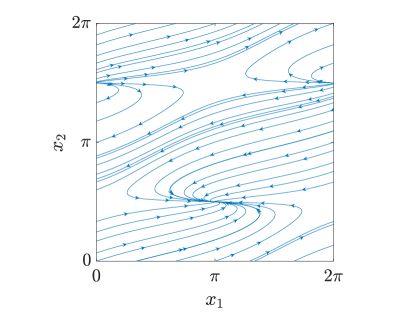
Refer to caption Refer to caption

Figure 7: Two-dimensional advection equation (97). (a) Characteristic curves associated associated with the PDE and (b) and divergence of the velocity field that advects the solution (b). Clearly, the flow depicted in (a) is not volume-preserving.

.

As is well known, the PDE (97) can be reduced to the trivial ODE du/dt=0𝑑𝑢𝑑𝑡0du/dt=0 along the flow generated by the dynamical system (see, e.g., [54])

{dx1dt=sin(x1)+3cos(x2),dx2dt=cos(x2).\left\{\begin{aligned} \displaystyle\frac{dx_{1}}{dt}&=\sin(x_{1})+3\cos(x_{2}),\vspace{0.2cm}\\ \displaystyle\frac{dx_{2}}{dt}&=\cos(x_{2}).\end{aligned}\right. (98)

In Figure 7 we plot the phase portrait we obtained by solving (98) numerically for different initial conditions (x01,x02)Ωsubscript𝑥01subscript𝑥02Ω(x_{01},x_{02})\in\Omega. With the flow {x1(t,x01,x02),x1(t,x01,x02)}subscript𝑥1𝑡subscript𝑥01subscript𝑥02subscript𝑥1𝑡subscript𝑥01subscript𝑥02\{x_{1}(t,x_{01},x_{02}),x_{1}(t,x_{01},x_{02})\} available, we can write the analytical solution to (97) as

u(x1,x2,t)=exp[sin(x01(x1,x2,t)+x02(x1,x2,t))],𝑢subscript𝑥1subscript𝑥2𝑡subscript𝑥01subscript𝑥1subscript𝑥2𝑡subscript𝑥02subscript𝑥1subscript𝑥2𝑡u(x_{1},x_{2},t)=\exp\left[\sin(x_{01}(x_{1},x_{2},t)+x_{02}(x_{1},x_{2},t))\right], (99)

where {x01(x1,x2,t),x02(x1,x2,t)}subscript𝑥01subscript𝑥1subscript𝑥2𝑡subscript𝑥02subscript𝑥1subscript𝑥2𝑡\{x_{01}(x_{1},x_{2},t),x_{02}(x_{1},x_{2},t)\} denotes the inverse flow. The semi-analytical solution (99) is plotted in the first row of Figure 8 at different times. Next, we compute the solution to (97) using the DO-TT method we proposed in Section 4. To this end, we first perform a bi-orthogonal decomposition of the initial condition u(x1,x2,0)𝑢subscript𝑥1subscript𝑥20u(x_{1},x_{2},0) in (97) with threshold set to σ=1013𝜎superscript1013\sigma=10^{-13} (see Section 2.4). This yields 171717 modes (ψi1(1),ψi1(2))i1=117superscriptsubscriptsubscriptsuperscript𝜓1subscript𝑖1subscriptsuperscript𝜓2subscript𝑖1subscript𝑖1117(\psi^{(1)}_{i_{1}},\psi^{(2)}_{i_{1}})_{i_{1}=1}^{17}, each of which is collocated on an evenly-spaced grid with 257257257 nodes in [0,2π]02𝜋[0,2\pi]. The DO-TT system associated with the PDE (97) is

ψj(2)tsubscriptsuperscript𝜓2𝑗𝑡\displaystyle\frac{\partial\psi^{(2)}_{j}}{\partial t} =i1=1r1{sin(x1)ψi1(1)x1ψj(1)ψi1(2)+3ψi1(1)x1ψj(1)ψi1(2)cos(x2)}+cos(x2)ψj(2)x2,absentsuperscriptsubscriptsubscript𝑖11subscript𝑟1delimited-⟨⟩subscript𝑥1subscriptsuperscript𝜓1subscript𝑖1subscript𝑥1subscriptsuperscript𝜓1𝑗subscriptsuperscript𝜓2subscript𝑖13delimited-⟨⟩subscriptsuperscript𝜓1subscript𝑖1subscript𝑥1subscriptsuperscript𝜓1𝑗subscriptsuperscript𝜓2subscript𝑖1subscript𝑥2subscript𝑥2subscriptsuperscript𝜓2𝑗subscript𝑥2\displaystyle=\sum_{i_{1}=1}^{r_{1}}\left\{\langle\sin(x_{1})\frac{\partial\psi^{(1)}_{i_{1}}}{\partial x_{1}}\psi^{(1)}_{j}\rangle\psi^{(2)}_{i_{1}}+3\langle\frac{\partial\psi^{(1)}_{i_{1}}}{\partial x_{1}}\psi^{(1)}_{j}\rangle\psi^{(2)}_{i_{1}}\cos(x_{2})\right\}+\cos(x_{2})\frac{\partial\psi^{(2)}_{j}}{\partial x_{2}}, (100)
p=1r1ψj(2)ψp(2)ψp(1)tsuperscriptsubscript𝑝1subscript𝑟1delimited-⟨⟩subscriptsuperscript𝜓2𝑗subscriptsuperscript𝜓2𝑝subscriptsuperscript𝜓1𝑝𝑡\displaystyle\sum_{p=1}^{r_{1}}\langle\psi^{(2)}_{j}\psi^{(2)}_{p}\rangle\frac{\partial\psi^{(1)}_{p}}{\partial t} =i1=1r1{sin(x1)ψi1(1)x1ψi1(2)ψj(2)+3ψi1(1)x1cos(x2)ψi1(2)ψj(2)+\displaystyle=\sum_{i_{1}=1}^{r_{1}}\left\{\sin(x_{1})\frac{\partial\psi^{(1)}_{i_{1}}}{\partial x_{1}}\langle\psi^{(2)}_{i_{1}}\psi^{(2)}_{j}\rangle+3\frac{\partial\psi^{(1)}_{i_{1}}}{\partial x_{1}}\langle\cos(x_{2})\psi_{i_{1}}^{(2)}\psi_{j}^{(2)}\rangle+\right.
ψi1(1)cos(x2)ψi1(2)x2ψj(2)p=1r1ψp(1)[sin(x1)ψi1(1)x1ψp(1)ψi1(2)ψj(2)\displaystyle\psi_{i_{1}}^{(1)}\langle\cos(x_{2})\frac{\partial\psi^{(2)}_{i_{1}}}{\partial x_{2}}\psi^{(2)}_{j}\rangle-\sum_{p=1}^{r_{1}}\psi^{(1)}_{p}\left[\langle\sin(x_{1})\frac{\partial\psi^{(1)}_{i_{1}}}{\partial x_{1}}\psi^{(1)}_{p}\rangle\langle\psi^{(2)}_{i_{1}}\psi^{(2)}_{j}\rangle\right.
+3ψi1(1)x1ψp(1)cos(x2)ψi1(2)ψj(2)+ψi1(1)ψp(1)cos(x2)ψi1(2)x2ψj(2)]}.\displaystyle\left.\left.+3\langle\frac{\partial\psi^{(1)}_{i_{1}}}{\partial x_{1}}\psi^{(1)}_{p}\rangle\langle\cos(x_{2})\psi_{i_{1}}^{(2)}\psi_{j}^{(2)}\rangle+\langle\psi_{i_{1}}^{(1)}\psi^{(1)}_{p}\rangle\langle\cos(x_{2})\frac{\partial\psi^{(2)}_{i_{1}}}{\partial x_{2}}\psi^{(2)}_{j}\rangle\right]\right\}.

In a Fourier spectral collocation setting [29], the partial derivatives /x1subscript𝑥1\partial/\partial x_{1}, /x2subscript𝑥2\partial/\partial x_{2} and the inner products can be easily represented by one-dimensional spectral differentiation matrices, and one-dimensional Fourier quadrature rules [29]. This allows us to transforms the PDE system (100) into a system of nonlinear ODEs with 2×r1×2562subscript𝑟12562\times r_{1}\times 256 equations. It is worthwhile emphasizing that the DO-TT system (100) is nonlinear even though the PDE (97) is linear. The nonlinearity is related to the fact that we implicitly project the solution back on a tensor manifold with constant rank r1subscript𝑟1r_{1} at each time. As we pointed out in Section 4, projecting on a tensor manifold with constant rank is a nonlinear operation. The system (100) is solved numerically by inverting the matrix Cjk(t)=ψj(2)ψk(2)subscript𝐶𝑗𝑘𝑡delimited-⟨⟩subscriptsuperscript𝜓2𝑗subscriptsuperscript𝜓2𝑘C_{jk}(t)=\langle\psi^{(2)}_{j}\psi^{(2)}_{k}\rangle (assuming it is non-singular) at each time step, and an explicit RK4 scheme with time step Δt=103Δ𝑡superscript103\Delta t=10^{-3}. We ran one simulation with constant rank r1=17subscript𝑟117r_{1}=17, two adaptive simulations using the pseudo-inverse (PI) technique proposed in [4] for addition of modes, and one adaptive simulation using our Algorithm 2 in Section 4.1. In Figure 8 we compare the time snapshots of the constant rank DO-TT solution (r1=17subscript𝑟117r_{1}=17) with the semi-analytical solution (99).

t=0.0𝑡0.0t=0.0                                                  t=0.5𝑡0.5t=0.5                                                  t=1.0𝑡1.0t=1.0

Method of characteristics Refer to caption Refer to caption Refer to caption

DO-TT (rank 17) Refer to caption Refer to caption Refer to caption

Pointwise error Refer to caption Refer to caption Refer to caption

Figure 8: Time snapshots of the solution to the PDE (97) obtained using Method of Characteristics and the proposed Dynamically Orthogonal Tensor Train (DO-TT) method with constant rank (r1=17subscript𝑟117r_{1}=17). We also plot the maximum pointwise error between the two solutions.

In Figure 12 we plot the time-dependent L2(Ω)superscript𝐿2ΩL^{2}(\Omega) errors between various DO-TT simulations and the semi-analytical solution (99). It is seen that the simulation with constant rank has an error slope that increases substantially around t=0.5𝑡0.5t=0.5. This suggests that 171717 DO-TT modes are no longer sufficient to represent the solution (99) for t>0.5𝑡0.5t>0.5. This can also be also seen from the fact that the DO-TT spectrum tends to flatten out in time (Figure 9), suggesting that each of the 171717 modes is picking up more and more energy. To overcome this problem, and therefore control the error growth in time, we implemented the adaptive algorithm for mode addition/removal proposed in [4], and compared it with our Algorithm 2 in Section 4.1 (Algorithm 2). As it is seen in Figure 11, such algorithm can indeed control the temporal growth of the DO-TT spectrum, hence the overall error (see Figure 12). Each time modes are added using our Algorithm 2 (Section 4.1), there is a re-orthogonalization process which can yield a discontinuity in the temporal evolution of each mode (see Figure 11). In practice, the DO-TT system is re-started from a new initial condition after such re-orthogonalization. This does is not affect the solution, nor creates any temporal discontinuity or error jump (see Figure 12).
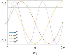
     t=0.0𝑡0.0t=0.0                                            t=0.5𝑡0.5t=0.5                                              t=1.0𝑡1.0t=1.0

Refer to caption Refer to caption Refer to caption

Refer to caption Refer to caption Refer to caption

λi1subscript𝜆subscript𝑖1\lambda_{i_{1}} Refer to caption Refer to caption Refer to caption

Figure 9: First four modes of the constant-rank (r1=17subscript𝑟117r_{1}=17) DO-TT representation of the solution to the PDE (97), and corresponding spectrum. Shown are results at times t=0.0𝑡0.0t=0.0, t=0.5𝑡0.5t=0.5 and t=1.0𝑡1.0t=1.0.

     t=0.0𝑡0.0t=0.0                                            t=0.5𝑡0.5t=0.5                                              t=1.0𝑡1.0t=1.0

Refer to caption Refer to caption Refer to caption

Refer to caption Refer to caption Refer to caption

λi1subscript𝜆subscript𝑖1\lambda_{i_{1}} Refer to caption Refer to caption Refer to caption

Figure 10: First four modes of the adaptive-rank DO-TT representation of the solution to (97), and corresponding spectrum. The adaptive expansion is computed by using our Algorithm 2 in Section 4.1. Shown are results at times t=0.0𝑡0.0t=0.0, t=0.5𝑡0.5t=0.5 and t=1.0𝑡1.0t=1.0. It is seen that the proposed algorithm can control the spectral decay at t=1𝑡1t=1 (compare the spectra in the last row of this Figure with the spectra in Figure 9).

   ψ2(2)subscriptsuperscript𝜓22\psi^{(2)}_{2}                                                                             ψ3(2)subscriptsuperscript𝜓23\psi^{(2)}_{3}

Refer to caption          Refer to caption

Figure 11: Adaptive DO-TT simulation of the PDE (97). Time evolution of the modes ψ2(2)superscriptsubscript𝜓22\psi_{2}^{(2)} and ψ3(2)superscriptsubscript𝜓32\psi_{3}^{(2)} we obtained by using Algorithm 2 in Section 4.1. In particular, here we add one mode at time t=0.5𝑡0.5t=0.5, t=0.55𝑡0.55t=0.55, t=0.6𝑡0.6t=0.6, t=0.65𝑡0.65t=0.65, t=0.7𝑡0.7t=0.7, t=0.75𝑡0.75t=0.75, t=0.8𝑡0.8t=0.8, t=0.825𝑡0.825t=0.825, t=0.85𝑡0.85t=0.85, t=0.9𝑡0.9t=0.9 (10 modes total). When a new mode is added, there is a re-orthogonalization process that can yield a discontinuity in the temporal evolution of each mode. In practice, the DO-TT system is re-started from a new initial condition after such re-orthogonalization takes place. This does not create any temporal discontinuity in the solution, nor any error jump (see Figure 12).
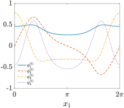
Refer to caption

Figure 12: Two-dimensional hyperbolic PDE (97). Time-dependent L2(Ω)superscript𝐿2ΩL^{2}(\Omega) errors between various DO-TT simulations and the semi-analytical solution (99). In particular, we plot the constant rank solution obtained by setting r1=17subscript𝑟117r_{1}=17 in (100) (dashed line); the DO-TT solution we obtained by adding one extra mode at t=0.5𝑡0.5t=0.5, t=0.55𝑡0.55t=0.55, t=0.6𝑡0.6t=0.6, t=0.65𝑡0.65t=0.65, t=0.7𝑡0.7t=0.7, t=0.75𝑡0.75t=0.75 (6 extra modes total) using the pseudo-inverse (PI) algorithm proposed in [4]; the DO-TT solution we obtained by adding one extra mode at t=0.5𝑡0.5t=0.5, t=0.55𝑡0.55t=0.55, t=0.6𝑡0.6t=0.6, t=0.65𝑡0.65t=0.65, t=0.7𝑡0.7t=0.7, t=0.75𝑡0.75t=0.75, t=0.8𝑡0.8t=0.8, t=0.825𝑡0.825t=0.825, t=0.85𝑡0.85t=0.85, t=0.9𝑡0.9t=0.9 using the pseudo-inverse algorithm (dashed line) and our Algorithm 2 in Section 4.1.

5.1.2 Four-dimensional hyperbolic PDE

Let us consider the following four-dimensional linear hyperbolic PDE

{u(𝒙,t)t=i,j=14cijfj(xj)u(𝒙,t)xiu(𝒙,0)=exp[110sin(x1+x2+x3+x4)]cases𝑢𝒙𝑡𝑡superscriptsubscript𝑖𝑗14subscript𝑐𝑖𝑗subscript𝑓𝑗subscript𝑥𝑗𝑢𝒙𝑡subscript𝑥𝑖otherwise𝑢𝒙0110subscript𝑥1subscript𝑥2subscript𝑥3subscript𝑥4otherwise\begin{cases}\displaystyle\frac{\partial{u(\bm{x},t)}}{\partial t}=\sum_{i,j=1}^{4}c_{ij}f_{j}(x_{j})\frac{\partial u(\bm{x},t)}{\partial x_{i}}\vspace{0.1cm}\\ \displaystyle u(\bm{x},0)=\exp\left[-\frac{1}{10}\sin(x_{1}+x_{2}+x_{3}+x_{4})\right]\end{cases} (101)

in the spatial domain Ω=[0,2π]4Ωsuperscript02𝜋4\Omega=[0,2\pi]^{4}, with periodic boundary conditions. In equation (101) cijsubscript𝑐𝑖𝑗c_{ij} are real numbers and fj(xj)subscript𝑓𝑗subscript𝑥𝑗f_{j}(x_{j}) are real-valued functions. The system of DO-TT evolution equations (94) can be explicitly written for the linear PDE (101). Such system is rather complicated, and therefore not presented here. For numerical demonstration, we set the coefficient matrix cijsubscript𝑐𝑖𝑗c_{ij} as

𝒄=[00.500000.3000010.5000]𝒄matrix00.500000.3000010.5000\bm{c}=\begin{bmatrix}0&0.5&0&0\\ 0&0&-0.3&0\\ 0&0&0&-1\\ 0.5&0&0&0\end{bmatrix}

and consider the following functions

f1(x1)=sin(x1),f2(x2)=cos(2x2),f3(x3)=sin(3x3),f4(x4)=cos(4x4).formulae-sequencesubscript𝑓1subscript𝑥1subscript𝑥1formulae-sequencesubscript𝑓2subscript𝑥22subscript𝑥2formulae-sequencesubscript𝑓3subscript𝑥33subscript𝑥3subscript𝑓4subscript𝑥44subscript𝑥4\displaystyle f_{1}(x_{1})=\sin(x_{1}),\qquad f_{2}(x_{2})=\cos(2x_{2}),\qquad f_{3}(x_{3})=\sin(3x_{3}),\qquad f_{4}(x_{4})=\cos(4x_{4}).

This yields non-trivial dynamics (cijsubscript𝑐𝑖𝑗c_{ij} is not diagonal). We solve the DO-TT system (94) numerically using a Fourier spectral collocation method with 202020 Fourier points in each variable xisubscript𝑥𝑖x_{i}, and RK4 time integration with Δt=103Δ𝑡superscript103\Delta t=10^{-3}. To this end, we first decompose the four-dimensional initial condition in (101) with the bi-orthogonal method we discussed in Section 2.1. Specifically, we consider the space H0(Ω)=L2(Ω)superscript𝐻0Ωsubscript𝐿2ΩH^{0}(\Omega)=L_{2}(\Omega) and set the eigenvalue threshold to σ=1010𝜎superscript1010\sigma=10^{-10}. This yields the following hierarchical ranks

r1=9,r2=[122222222],r3=[122222222022222222]T,formulae-sequencesubscript𝑟19formulae-sequencesubscript𝑟2matrix122222222subscript𝑟3superscriptmatrix122222222022222222𝑇\displaystyle r_{1}=9,\qquad r_{2}=\begin{bmatrix}1&2&2&2&2&2&2&2&2\end{bmatrix},\qquad r_{3}=\begin{bmatrix}1&2&2&2&2&2&2&2&2\\ 0&2&2&2&2&2&2&2&2\end{bmatrix}^{T}, (102)

which we keep constant throughout the simulation. In other words, here we do not perform adaptive addition/removal of DO-TT modes as we did in the previous PDE example (Eqs. (97) and (100)). In Figure 13 we plot the time evolution of a few representative DO-TT modes.
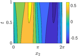
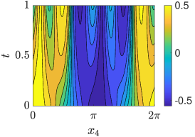
   ψ21(2)superscriptsubscript𝜓212\psi_{21}^{(2)}                                                      ψ211(4)subscriptsuperscript𝜓4211\psi^{(4)}_{211}                                                      ψ311(4)subscriptsuperscript𝜓4311\psi^{(4)}_{311}

Refer to caption Refer to caption Refer to caption

Figure 13: Time evolution of a few representative DO-TT modes generated by the four-dimensional hyperbolic initial/boundary value problem (101).

It is seen that as time evolves the spatial frequency of such modes increases which suggests that the hyperbolic dynamics activate higher spatial frequencies in the spectral representation of the PDE solution. This is shown in Figure 14, where we plot one section of the solution to the initial value problem (101) we obtained with the method of characteristics (benchmark solution), and the solution we obtained with the DO-TT propagator. It is seen that even with the very few hierarchical ranks summarized in (102) we were able to resolve the 4D solution to a reasonable accuracy (see Figure 15(a)).

t=0.0𝑡0.0t=0.0                                                  t=0.5𝑡0.5t=0.5                                                  t=1.0𝑡1.0t=1.0

Method of characteristics Refer to caption Refer to caption Refer to caption

DO-TT Refer to caption Refer to caption Refer to caption

Pointwise error Refer to caption Refer to caption Refer to caption

Figure 14: Time snapshots of a 2D slice (x1=2.9568subscript𝑥12.9568x_{1}=2.9568, x2=2.9568subscript𝑥22.9568x_{2}=2.9568) of the solution to the four-dimensional PDE (101) obtained using method of characteristics (benchmark solution), and the DO-TT propagator with hierarchical ranks (102). We also plot the maximum pointwise error between the two solutions.

    (a)                                                                                       (b)

Refer to caption Refer to caption

Figure 15: Time-dependent L2(Ω)superscript𝐿2ΩL^{2}(\Omega) error of the DO-TT approximation of the solution to the four-dimensional PDE (101) (a), and the fifty-dimensional PDE (103) (b). In (a) we computed the DO-TT error relative to an accurate benchmark solution constructed with the method of characteristics. In (b) we used the analytical solution (108).

5.2 Fifty-dimensional hyperbolic PDE

Let us consider the following fifty-dimensional hyperbolic problem

{u(𝒙,t)t=j=150fj(xj)u(𝒙,t)xju(𝒙,0)=j=150ψ0(j)(xj)cases𝑢𝒙𝑡𝑡superscriptsubscript𝑗150subscript𝑓𝑗subscript𝑥𝑗𝑢𝒙𝑡subscript𝑥𝑗otherwise𝑢𝒙0superscriptsubscriptproduct𝑗150superscriptsubscript𝜓0𝑗subscript𝑥𝑗otherwise\begin{cases}\displaystyle\frac{\partial u(\bm{x},t)}{\partial t}=\sum_{j=1}^{50}f_{j}(x_{j})\frac{\partial u(\bm{x},t)}{\partial x_{j}}\vspace{0.1cm}\\ {u}(\bm{x},0)=\displaystyle\prod_{j=1}^{50}\psi_{0}^{(j)}(x_{j})\end{cases} (103)

subject to periodic boundary conditions in the hyper-cube Ω=[0,2π]50Ωsuperscript02𝜋50\Omega=[0,2\pi]^{50}. It is easy to show that the solution to (103) is rank-one for all t0𝑡0t\geq 0. Correspondingly, we look for a rank-one DO-TT solution of the form

u~=j=150ψ(j)(t).~𝑢superscriptsubscriptproduct𝑗150superscript𝜓𝑗𝑡\tilde{u}=\prod_{j=1}^{50}\psi^{(j)}(t). (104)

By substituting (104) into (103) and imposing DO orthogonality conditions at each level of the binary tree yields the DO-TT propagator

ψ(j)tsuperscript𝜓𝑗𝑡\displaystyle\frac{\partial\psi^{(j)}}{\partial t} =fj(xj)ψ(j)xjfj(xj)ψ(j)ψ(j)xjψ(j),j=1,2,,49formulae-sequenceabsentsubscript𝑓𝑗subscript𝑥𝑗superscript𝜓𝑗subscript𝑥𝑗subscript𝑓𝑗subscript𝑥𝑗superscript𝜓𝑗delimited-⟨⟩superscript𝜓𝑗subscript𝑥𝑗superscript𝜓𝑗𝑗1249\displaystyle=f_{j}(x_{j})\frac{\partial\psi^{(j)}}{\partial x_{j}}-f_{j}(x_{j})\psi^{(j)}\langle\frac{\partial\psi^{(j)}}{\partial x_{j}}\psi^{(j)}\rangle\ ,\qquad j=1,2,\ldots,49 (105)
ψ(50)tsuperscript𝜓50𝑡\displaystyle\frac{\partial\psi^{(50)}}{\partial t} =j=149fj(xj)ψ(j)xjψ(j)ψ(50).absentsuperscriptsubscript𝑗149subscript𝑓𝑗subscript𝑥𝑗delimited-⟨⟩superscript𝜓𝑗subscript𝑥𝑗superscript𝜓𝑗superscript𝜓50\displaystyle=\sum_{j=1}^{49}f_{j}(x_{j})\langle\frac{\partial\psi^{(j)}}{\partial x_{j}}\psi^{(j)}\rangle\psi^{(50)}.

Note that this system is nonlinear. Specifically, the first 49 equations are uncoupled, while the 50th one is coupled with the entire system. We set the coefficients fj(xj)=jsubscript𝑓𝑗subscript𝑥𝑗𝑗f_{j}(x_{j})=j, i.e., constant, and the components of the initial condition as

ψ0(j)(xj)=sin(xj)π,j=1,,49,ψ0(50)(x50)=107(3+sin(x50)),formulae-sequencesuperscriptsubscript𝜓0𝑗subscript𝑥𝑗subscript𝑥𝑗𝜋formulae-sequence𝑗149superscriptsubscript𝜓050subscript𝑥50superscript1073subscript𝑥50\displaystyle\psi_{0}^{(j)}(x_{j})=\frac{\sin(x_{j})}{\sqrt{\pi}},\quad j=1,\ldots,49,\qquad\psi_{0}^{(50)}(x_{50})=10^{7}(3+\sin(x_{50})), (106)

which satisfy the bi-orthogonality condition. The analytical solution to (103) is easily obtained as

u=j=150ψ0(j)(xj+jt).𝑢superscriptsubscriptproduct𝑗150superscriptsubscript𝜓0𝑗subscript𝑥𝑗𝑗𝑡u=\prod_{j=1}^{50}\psi_{0}^{(j)}(x_{j}+jt). (107)

As before, we solved the DO-TT system (105) using a Fourier spectral collocation method with 606060 Fourier points in each variable xjsubscript𝑥𝑗x_{j}, and RK4 time integration with Δt=103Δ𝑡superscript103\Delta t=10^{-3}. The temporal evolution of a few representative DO-TT modes is shown in Figure 16.

ψ(1)superscript𝜓1\psi^{(1)}                                                      ψ(25)superscript𝜓25\psi^{(25)}                                                      ψ(50)superscript𝜓50\psi^{(50)}

Refer to caption Refer to caption Refer to caption

Figure 16: Time evolution of a few representative DO-TT modes solving nonlinear PDE system (105). It is seen that all modes are traveling waves.

The L2(Ω)superscript𝐿2ΩL^{2}(\Omega) error between the analytical solution (107) and the DO-TT approximation (104) can be represented in terms of one-dimensional integrals as follows

uu~L2(Ω)2subscriptsuperscriptnorm𝑢~𝑢2superscript𝐿2Ω\displaystyle\left\|u-\tilde{u}\right\|^{2}_{L^{2}(\Omega)} =Ω(j=150ψ0(j)(xj+jt)j=150ψ(j)(t))2𝑑x1𝑑x50absentsubscriptΩsuperscriptsuperscriptsubscriptproduct𝑗150superscriptsubscript𝜓0𝑗subscript𝑥𝑗𝑗𝑡superscriptsubscriptproduct𝑗150superscript𝜓𝑗𝑡2differential-dsubscript𝑥1differential-dsubscript𝑥50\displaystyle=\int_{\Omega}\left(\prod_{j=1}^{50}\psi_{0}^{(j)}(x_{j}+jt)-\prod_{j=1}^{50}\psi^{(j)}(t)\right)^{2}dx_{1}\cdots dx_{50} (108)
=j=15002πψ0(j)(xj+jt)2𝑑xj+j=15002πψ(j)(t)2𝑑xj2j=15002πψ0(j)(xj+jt)ψ(j)(t)𝑑xj.absentsuperscriptsubscriptproduct𝑗150superscriptsubscript02𝜋superscriptsubscript𝜓0𝑗superscriptsubscript𝑥𝑗𝑗𝑡2differential-dsubscript𝑥𝑗superscriptsubscriptproduct𝑗150superscriptsubscript02𝜋superscript𝜓𝑗superscript𝑡2differential-dsubscript𝑥𝑗2superscriptsubscriptproduct𝑗150superscriptsubscript02𝜋subscriptsuperscript𝜓𝑗0subscript𝑥𝑗𝑗𝑡superscript𝜓𝑗𝑡differential-dsubscript𝑥𝑗\displaystyle=\prod_{j=1}^{50}\int_{0}^{2\pi}\psi_{0}^{(j)}(x_{j}+jt)^{2}dx_{j}+\prod_{j=1}^{50}\int_{0}^{2\pi}\psi^{(j)}(t)^{2}dx_{j}-2\prod_{j=1}^{50}\int_{0}^{2\pi}\psi^{(j)}_{0}(x_{j}+jt)\psi^{(j)}(t)dx_{j}.

This error is plotted in Figure 15(b) versus time. It is seen that the DO-TT propagator in this case is numerically exact.

5.3 Parabolic PDEs

In this Section we study DO-TT solution of constant-coefficients parabolic PDEs in periodic hypercubes. In contrast with the hyperbolic problems discussed in the previous Section, the solution in this case does not increase in rank throughout propagation. Rather, the solution smooths out over time and the rank tends to decrease. This implies that in order for the covariance matrices in the DO-TT system to remain invertible during propagation, a threshold must be set to dynamically remove modes, in particular when their energy becomes very small.

5.3.1 Four-dimensional parabolic PDE

Let us consider the four-dimensional initial value problem

{u(t,𝒙)t=j=142u(𝒙,t)xj2u(𝒙,0)=exp[110sin(x1+x2+x3+x4)]cases𝑢𝑡𝒙𝑡superscriptsubscript𝑗14superscript2𝑢𝒙𝑡superscriptsubscript𝑥𝑗2otherwise𝑢𝒙0110subscript𝑥1subscript𝑥2subscript𝑥3subscript𝑥4otherwise\begin{cases}\displaystyle\frac{\partial u(t,\bm{x})}{\partial t}=\sum_{j=1}^{4}\frac{\partial^{2}u(\bm{x},t)}{\partial x_{j}^{2}}\vspace{0.1cm}\\ \displaystyle{u}(\bm{x},0)=\exp\left[-\frac{1}{10}\sin(x_{1}+x_{2}+x_{3}+x_{4})\right]\end{cases} (109)

in the spatial domain Ω=[0,2π]4Ωsuperscript02𝜋4\Omega=[0,2\pi]^{4}, with periodic boundary conditions. Note that here we set the same initial condition as in the hyperbolic PDE (101). In this case, however, the solution decays to zero because of diffusion. Hence, we expect that the DO-TT solution rank decays in time, instead of increasing. Applying the Fourier transform []delimited-[]\mathcal{F}[\cdot] to (109), yields the linear ODE

{du^(t,𝝎)dt=j=14ωj2u^(t,𝝎)u^(𝝎,0)=[exp(110sin(x1+x2+x3+x4))](𝝎)cases𝑑^𝑢𝑡𝝎𝑑𝑡superscriptsubscript𝑗14superscriptsubscript𝜔𝑗2^𝑢𝑡𝝎otherwise^𝑢𝝎0delimited-[]110subscript𝑥1subscript𝑥2subscript𝑥3subscript𝑥4𝝎otherwise\begin{cases}\displaystyle\frac{d\hat{u}(t,\bm{\omega})}{dt}=-\sum_{j=1}^{4}\omega_{j}^{2}\hat{u}(t,\bm{\omega})\vspace{0.1cm}\\ \displaystyle\hat{u}(\bm{\omega},0)=\mathcal{F}\left[\exp\left(-\frac{1}{10}\sin(x_{1}+x_{2}+x_{3}+x_{4})\right)\right](\bm{\omega})\end{cases} (110)

which can be solved analytically or numerically to obtain a benchmark solution to (109). With such benchmark solution available, we can study the accuracy of the DO-TT propagator. To this end, we first compute the bi-orthogonal decomposition of the initial condition in (109) as we have done in Section 5.1.2, with threshold set to σ=1010𝜎superscript1010\sigma=10^{-10}. This yields the the hierarchical ranks (102), as before. In Figure 17 we plot L2(Ω)superscript𝐿2ΩL^{2}(\Omega) error of the DO-TT approximation of the solution to (109) relative to the benchmark solution obtained via Fourier transform. It is seen that, contrary to hyperbolic problems, diffusion promotes a low-rank structure of the solution.

(a)                                                                                       (b)

Refer to caption Refer to caption

Figure 17: (a) Temporal evolution of the level-1 rank in the DO-TT approximation of the solution to four-dimensional diffusion problem (109). It is seen that that diffusion promotes a low-rank structure of the solution. In (b) we plot L2(Ω)superscript𝐿2ΩL^{2}(\Omega) error of the DO-TT approximation relative to the benchmark solution, which is obtained via Fourier transform.

This means that the energy of the DO-TT modes tends to decrease in time, which implies that the covariance matrix at the left hand side of the DO-TT propagator can become numerically singular in time. To avoid such singularities we introduce a threshold ϵ=1010italic-ϵsuperscript1010\epsilon=10^{-10} on the eigenvalues of the level-1 TT binary tree, i.e., λi1subscript𝜆subscript𝑖1\lambda_{i_{1}}, to determine whether we should decrease the leading rank r1subscript𝑟1r_{1}. Specifically, if λr1<ϵsubscript𝜆subscript𝑟1italic-ϵ\lambda_{r_{1}}<\epsilon then r1=r11subscript𝑟1subscript𝑟11r_{1}=r_{1}-1. For this example, thresholding only the first level is sufficient to avoid singular covariance matrices at all levels of the TT binary tree. In Figure 17 we see that each time we remove one mode we have that the relative error jumps. Note however, that it immediately decays again with a rate that is inversely proportional to the number of the DO-TT modes kept in the series expansion.

5.4 Fifty-dimensional parabolic PDE

The last problem we consider is a fifty-dimensional constant-coefficient diffusion problem with rank-one initial condition

{u(𝒙,t)t=j=1502u(𝒙,t)xj2u(𝒙,t)=j=150ψ0(j)(xj)cases𝑢𝒙𝑡𝑡superscriptsubscript𝑗150superscript2𝑢𝒙𝑡superscriptsubscript𝑥𝑗2otherwise𝑢𝒙𝑡superscriptsubscriptproduct𝑗150superscriptsubscript𝜓0𝑗subscript𝑥𝑗otherwise\begin{cases}\displaystyle\frac{\partial u(\bm{x},t)}{\partial t}=\sum_{j=1}^{50}\frac{\partial^{2}u(\bm{x},t)}{\partial x_{j}^{2}}\vspace{0.1cm}\\ {u}(\bm{x},t)=\displaystyle\prod_{j=1}^{50}\psi_{0}^{(j)}(x_{j})\end{cases} (111)

in the spatial domain Ω=[0,2π]50Ωsuperscript02𝜋50\Omega=[0,2\pi]^{5}0, with periodic boundary conditions. The analytical solution can be obtained by using the method of separation of variables [49] as

u=j=150ψ0(j)e50t.𝑢superscriptsubscriptproduct𝑗150subscriptsuperscript𝜓𝑗0superscript𝑒50𝑡u=\prod_{j=1}^{50}\psi^{(j)}_{0}e^{-50t}. (112)

Hence, it is a rank-one solution. Correspondingly, we look for a rank-one DO-TT solution of the form

u~=j=150ψ(j)(t),~𝑢superscriptsubscriptproduct𝑗150superscript𝜓𝑗𝑡\tilde{u}=\prod_{j=1}^{50}\psi^{(j)}(t)\ , (113)

where the modes ψ(j)(t)superscript𝜓𝑗𝑡\psi^{(j)}(t) satisfy the DO-TT system of evolution equations

ψ(j)tsuperscript𝜓𝑗𝑡\displaystyle\frac{\partial\psi^{(j)}}{\partial t} =2ψ(j)xj2ψ(j)2ψ(j)xj2ψ(j),j=1,2,,49,formulae-sequenceabsentsuperscript2superscript𝜓𝑗superscriptsubscript𝑥𝑗2superscript𝜓𝑗delimited-⟨⟩superscript2superscript𝜓𝑗superscriptsubscript𝑥𝑗2superscript𝜓𝑗𝑗1249\displaystyle=\frac{\partial^{2}\psi^{(j)}}{\partial x_{j}^{2}}-\psi^{(j)}\langle\frac{\partial^{2}\psi^{(j)}}{\partial x_{j}^{2}}\psi^{(j)}\rangle\ ,\qquad j=1,2,\ldots,49\ , (114)
ψ(50)tsuperscript𝜓50𝑡\displaystyle\frac{\partial\psi^{(50)}}{\partial t} =j=1492ψ(j)xj2ψ(j)ψ(50).absentsuperscriptsubscript𝑗149delimited-⟨⟩superscript2superscript𝜓𝑗superscriptsubscript𝑥𝑗2superscript𝜓𝑗superscript𝜓50\displaystyle=\sum_{j=1}^{49}\langle\frac{\partial^{2}\psi^{(j)}}{\partial x_{j}^{2}}\psi^{(j)}\rangle\psi^{(50)}.

We set the initial condition in (111) as

ψ0(j)=sin(xj)π,j=1,,49,ψ0(50)=107sin(x50),formulae-sequencesuperscriptsubscript𝜓0𝑗subscript𝑥𝑗𝜋formulae-sequence𝑗149superscriptsubscript𝜓050superscript107subscript𝑥50\displaystyle\psi_{0}^{(j)}=\frac{\sin(x_{j})}{\sqrt{\pi}},\quad j=1,\ldots,49\ ,\qquad\psi_{0}^{(50)}=10^{7}\sin(x_{50})\ , (115)

which satisfy the orthogonality conditions. As before, we solved the system (114) using Fourier spectral collocation with 60 nodes in each variable xjsubscript𝑥𝑗x_{j} and RK4 time integration with Δt=103Δ𝑡superscript103\Delta t=10^{-3}. In Figure 18 we plot the temporal evolution of a few representative DO-TT modes. As expected, they all decay to zero.
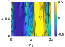
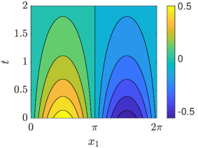
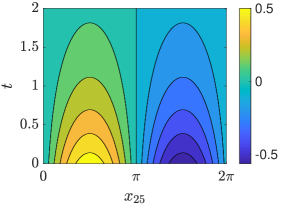
    ψ(1)superscript𝜓1\psi^{(1)}                                                      ψ(25)superscript𝜓25\psi^{(25)}                                                      ψ(50)superscript𝜓50\psi^{(50)}

Refer to caption Refer to caption Refer to caption

Figure 18: Fifty-dimensional diffusion problem (111). Time evolution of a few representative DO-TT modes appearing in the rank-one expansion of solution (113). As expected, all modes decay to zero.

Finally in Figure 19 we plot the time-dependent L2(Ω)superscript𝐿2ΩL^{2}(\Omega) error between the DO-TT solution (113) and the analytical solution (112). Such error can be expressed in terms of one-dimensional integrals as follows

uu~L2(Ω)2=subscriptsuperscriptnorm𝑢~𝑢2superscript𝐿2Ωabsent\displaystyle\left\|u-\tilde{u}\right\|^{2}_{L^{2}(\Omega)}= j=15002πψ0(j)(xj)2𝑑xje100t+j=15002πψ(j)(t)2𝑑xjsuperscriptsubscriptproduct𝑗150superscriptsubscript02𝜋superscriptsubscript𝜓0𝑗superscriptsubscript𝑥𝑗2differential-dsubscript𝑥𝑗superscript𝑒100𝑡limit-fromsuperscriptsubscriptproduct𝑗150superscriptsubscript02𝜋superscript𝜓𝑗superscript𝑡2differential-dsubscript𝑥𝑗\displaystyle\prod_{j=1}^{50}\int_{0}^{2\pi}\psi_{0}^{(j)}(x_{j})^{2}dx_{j}e^{-100t}+\prod_{j=1}^{50}\int_{0}^{2\pi}\psi^{(j)}(t)^{2}dx_{j}- (116)
2j=15002πψ0(j)(xj)ψ(j)(t)𝑑xje50t.2superscriptsubscriptproduct𝑗150superscriptsubscript02𝜋subscriptsuperscript𝜓𝑗0subscript𝑥𝑗superscript𝜓𝑗𝑡differential-dsubscript𝑥𝑗superscript𝑒50𝑡\displaystyle 2\prod_{j=1}^{50}\int_{0}^{2\pi}\psi^{(j)}_{0}(x_{j})\psi^{(j)}(t)dx_{j}e^{-50t}.

Refer to caption

Figure 19: Fifty-dimensional diffusion problem (111). L2(Ω)superscript𝐿2ΩL^{2}(\Omega) error between the DO-TT solution (113) and the analytical solution (112).

6 Summary

In this paper, we presented a new dynamically orthogonal tensor decomposition method to approximate multivariate functions and the solution to high-dimensional time-dependent nonlinear PDEs. The key idea relies on a hierarchical decomposition of the approximation space obtained by splitting the independent variables of the problem into disjoint subsets. This process, which can be conveniently be visualized in terms of binary trees, yields series expansions analogous to the classical tensor-train and hierarchical Tucker tensor formats. By enforcing dynamic orthogonality conditions at each level of binary tree, we obtained evolution equations for the orthogonal modes spanning each of the nested subspaces in the hierarchical decomposition. This allowed us to represent the temporal dynamics of high-dimensional functions, and compute the solution to high-dimensional time-dependent PDEs on a tensor manifold with constant rank. We also proposed a new algorithm for dynamic addition and removal of modes within each subspace, and demonstrated its effectiveness in numerical applications to hyperbolic and parabolic PDEs. The mathematical techniques and algorithms we presented in this paper can be readily applied to more general high-dimensional nonlinear systems and PDEs, such as the finite-dimensional approximation of nonlinear functionals and functional differential equations [63].

Acknowledgements This research was supported by the U.S. Army Research Office grant W911NF1810309.

References

  • [1] N. Aubry. On the hidden beauty of the proper orthogonal decomposition. Theoretical and Computational Fluid Dynamics, 2(5):339–352, 1991.
  • [2] N. Aubry, R. Guyonnet, and R. Lima. Spatiotemporal analysis of complex signals: theory and applications. J. Stat. Phys., 64(3-4):683–739, 1991.
  • [3] N. Aubry and R. Lima. Spatiotemporal and statistical symmetries. J. Stat. Phys., 81(3-4):793–828, 1995.
  • [4] H. Babaee, M. Choi, T. P. Sapsis, and G. E. Karniadakis. A robust bi-orthogonal/dynamically-orthogonal method using the covariance pseudo-inverse with application to stochastic flow problems. J. Comput. Phys., 344:303–319, 2017.
  • [5] M. Bachmayr, R. Schneider, and A. Uschmajew. Tensor networks and hierarchical tensors for the solution of high-dimensional partial differential equations. Foundations of Computational Mathematics, 16(6), 2016.
  • [6] J. Baldeaux and M. Gnewuch. Optimal randomized multilevel algorithms for infinite-dimensional integration on function spaces with ANOVA-type decomposition. SIAM J. Numer. Anal., 52(3):1128–1155, 2014.
  • [7] V. Barthelmann, E. Novak, and K. Ritter. High dimensional polynomial interpolation on sparse grids. Advances in Computational Mechanics, 12:273–288, 2000.
  • [8] R. Bertram and J. E. Rubin. Multi-timescale systems and fast-slow analysis. Math. Biosci., 287:105–121, 2017.
  • [9] A. M. P. Boelens, D. Venturi, and D. M. Tartakovsky. Parallel tensor methods for high-dimensional linear PDEs. J. Comput. Phys., 375:519–539, 2018.
  • [10] H. J. Bungartz and M. Griebel. Sparse grids. Acta Numerica, 13:147–269, 2004.
  • [11] Y. Cao, Z. Chen, and M. Gunzbuger. ANOVA expansions and efficient sampling methods for parameter dependent nonlinear PDEs. Int. J. Numer. Anal. Model., 6:256–273, 2009.
  • [12] Carlo Cercignani. The Boltzmann equation and its applications. Springer, 1988.
  • [13] M. Cheng, T. Y. Hou, and Z. Zhang. A dynamically bi-orthogonal method for time-dependent stochastic partial differential equations i: Derivation and algorithms. J. Comput. Phys., 242:843 – 868, 2013.
  • [14] M. Cheng, T. Y. Hou, and Z. Zhang. A dynamically bi-orthogonal method for time-dependent stochastic partial differential equations I: derivation and algorithms. J. Comput. Phys., 242:843–868, 2013.
  • [15] M. Cheng, T. Y. Hou, and Z. Zhang. A dynamically bi-orthogonal method for time-dependent stochastic partial differential equations II: adaptivity and generalizations. J. Comput. Phys., 242:753–776, 2013.
  • [16] F. Chinesta, R. Keunings, and A. Leygue. The Proper generalized decomposition for advanced numerical simulations. Springer, 2014.
  • [17] A. Chkifa, A. Cohen, and C. Schwab. High-dimensional adaptive sparse polynomial interpolation and applications to parametric PDEs. Found. Comput. Math., 14:601–633, 2014.
  • [18] H. Cho, D. Venturi, and G. E. Karniadakis. Numerical methods for high-dimensional probability density function equation. J. Comput. Phys, 315:817–837, 2016.
  • [19] M. Choi, T.P. Sapsis, and G.E. Karniadakis. On the equivalence of dynamically orthogonal and bi-orthogonal methods: theory and numerical simulations. J. Comput. Phys., 270:1–20, 2014.
  • [20] V. de Silva and L.-H. Lim. Tensor rank and ill-posedness of the best low-rank approximation problem. SIAM J. Matrix Anal. Appl., 30:1084–1127, 2008.
  • [21] J. Dick, F. Y. Kuo, and I. H. Sloan. High-dimensional integration: the quasi-Monte Carlo way. Acta Numerica, 22:133–288, 2013.
  • [22] A. Etter. Parallel ALS algorithm for solving linear systems in the hierarchical Tucker representation. SIAM J. Sci. Comput., 38(4):A2585–A2609, 2016.
  • [23] J. Foo and G. E. Karniadakis. Multi-element probabilistic collocation method in high dimensions. J. Comput. Phys., 229:1536–1557, 2010.
  • [24] L. Grasedyck. Hierarchical singular value decomposition of tensors. SIAM J. Matrix Anal. Appl., 31(4):2029–2054, 2009/10.
  • [25] L. Grasedyck, D. Kressner, and C. Tobler. A literature survey of low-rank tensor approximation techniques. GAMM-Mitt., 36(1):53–78, 2013.
  • [26] L. Grasedyck and C. Löbbert. Distributed hierarchical SVD in the hierarchical Tucker format. Numer. Linear Algebra Appl., 25(6):e2174, 2018.
  • [27] M. Griebel and G. Li. On the decay rate of the singular values of bivariate functions. SIAM J. Numer. Anal., 56(2):974–993, 2019.
  • [28] W. Hackbusch. Tensor spaces and numerical tensor calculus. Springer, 2012.
  • [29] J. S. Hesthaven, S. Gottlieb, and D. Gottlieb. Spectral methods for time-dependent problems. Cambridge University Press, Cambridge, 2007.
  • [30] E. Hopf. Statistical hydromechanics and functional calculus. J. Rat. Mech. Anal., 1(1):87–123, 1952.
  • [31] E. Hopf and E. W. Titt. On certain special solutions of the ϕitalic-ϕ\phi-equation of statistical hydrodynamics. J. Rat. Mech. Anal., 2(3):587–592, 1953.
  • [32] C. Itzykson and J. B. Zuber. Quantum field theory. Dover, 2005. Republication of the work originally published by McGraw-Hill, Inc., NY, 1980.
  • [33] R. V. Jensen. Functional integral approach to classical statistical dynamics. J. Stat. Phys., 25(2):183–210, 1981.
  • [34] B. Jouvet and R. Phythian. Quantum aspects of classical and statistical fields. Phys. Rev. A, 19:1350–1355, 1979.
  • [35] L. Karlsson, D. Kressner, and A. Uschmajew. Parallel algorithms for tensor completion in the CP format. Parallel compting, 57:222–234, 2016.
  • [36] T. Kato. Perturbation theory for linear operators. Classics in Mathematics. Springer-Verlag, Berlin, 1995. Reprint of the 1980 edition.
  • [37] B. N. Khoromskij. Tensor numerical methods for multidimensional PDEs: theoretical analysis and initial applications. In CEMRACS 2013–modelling and simulation of complex systems: stochastic and deterministic approaches, volume 48 of ESAIM Proc. Surveys, pages 1–28. EDP Sci., Les Ulis, 2015.
  • [38] O. Koch and C. Lubich. Dynamical tensor approximation. SIAM J. Matrix Anal. Appl., 31(5):2360–2375, 2010.
  • [39] T. Kolda and B. W. Bader. Tensor decompositions and applications. SIREV, 51:455–500, 2009.
  • [40] D. Kressner and C. Tobler. Algorithm 941: htucker – a Matlab toolbox for tensors in hierarchical Tucker format. ACM Transactions on Mathematical Software, 40(3):1–22, 2014.
  • [41] L. D. Lathauwer, B. D. Moor, and J. Vandewalle. A multilinear singular value decomposition. SIAM J. Matrix Anal. Appl., 21(4):1253–1278, 2000.
  • [42] G. Li and H. Rabitz. Regularized random-sampling high dimensional model representation (RS-HDMR). Journal of Mathematical Chemistry, 43(3):1207–1232, 2008.
  • [43] C. Lubich, B. Vandereycken, and A. Walach. Time integration of rank-constrained Tucker tensors. SIAM J. Numer. Anal., 56(3):1273–1290, 2018.
  • [44] G. Di Marco and L. Pareschi. Numerical methods for kinetic equations. Acta Numerica, 23:369–520, 2014.
  • [45] P. C. Martin, E. D. Siggia, and H. A. Rose. Statistical dynamics of classical systems. Phys. Rev. A, 8:423–437, 1973.
  • [46] A. S. Monin and A. M. Yaglom. Statistical Fluid Mechanics, Volume II: Mechanics of Turbulence. Dover, 2007.
  • [47] A. Narayan and J. Jakeman. Adaptive Leja sparse grid constructions for stochastic collocation and high-dimensional approximation. SIAM J. Sci. Comput., 36(6):A2952–A2983, 2014.
  • [48] I. V. Oseledets. Tensor-train decomposition. SIAM J. Sci. Comput., 33(5):2295––2317, 2011.
  • [49] M. N. Özişik. Heat conduction. John Wiley & Sons, second edition, 1993.
  • [50] R. Phythian. The functional formalism of classical statistical dynamics. J. Phys A: Math. Gen., 10(5):777–788, 1977.
  • [51] M. Raissi and G. E. Karniadakis. Hidden physics models: Machine learning of nonlinear partial differential equations. J. Comput. Phys., 357:125–141, 2018.
  • [52] M. Raissi, P. Perdikaris, and G. E. Karniadakis. Physics-informed neural networks: A deep learning framework for solving forward and inverse problems involving nonlinear partial differential equations. J. Comput. Phys., 378:606–707, 2019.
  • [53] M. Reed and B. Simon. Methods of modern mathematical physics. I. Academic Press, Inc. [Harcourt Brace Jovanovich, Publishers], New York, second edition, 1980. Functional analysis.
  • [54] H.-K. Rhee, R. Aris, and N. R. Amundson. First-order partial differential equations, volume 1: theory and applications of single equations. Dover, 2001.
  • [55] H. Risken. The Fokker-Planck equation: methods of solution and applications. Springer-Verlag, second edition, 1989. Mathematics in science and engineering, vol. 60.
  • [56] T. Rohwedder and A. Uschmajew. On local convergence of alternating schemes for optimization of convex problems in the tensor train format. SIAM J. Numer. Anal., 51(2):1134–1162, 2013.
  • [57] T. P. Sapsis and P. F.J.Lermusiaux. Dynamically orthogonal field equations for continuous stochastic dynamical systems. Phys. D, 238(23-24):2347–2360, 2009.
  • [58] R. Schneider and A. Uschmajew. Approximation rates for the hierarchical tensor format in periodic Sobolev spaces. J. Complexity, 30(2):56–71, 2014.
  • [59] C. Da Silva and F. J. Herrmann. Optimization on the Hierarchical Tucker manifold – applications to tensor completion. Linear Algebra and its Applications, 481:131–173, 2015.
  • [60] A. Uschmajew and B. Vandereycken. The geometry of algorithms using hierarchical tensors. Linear Algebra Appl., 439(1):133–166, 2013.
  • [61] D. Venturi. On proper orthogonal decomposition of randomly perturbed fields with applications to flow past a cylinder and natural convection over a horizontal plate. J. Fluid Mech., 559:215–254, 2006.
  • [62] D. Venturi. A fully symmetric nonlinear biorthogonal decomposition theory for random fields. Phys. D, 240(4-5):415–425, 2011.
  • [63] D. Venturi. The numerical approximation of nonlinear functionals and functional differential equations. Physics Reports, 732:1–102, 2018.
  • [64] D. Venturi, T. P. Sapsis, H. Cho, and G. E. Karniadakis. A computable evolution equation for the joint response-excitation probability density function of stochastic dynamical systems. Proc. R. Soc. A, 468(2139):759–783, 2012.
  • [65] D. Venturi, X. Wan, and G. E. Karniadakis. Stochastic low-dimensional modelling of a random laminar wake past a circular cylinder. J. Fluid Mech., 606:339–367, 2008.
  • [66] Y. Zhu, N. Zabaras, P.-S. Koutsourelakis, and P. Perdikaris. Physics-constrained deep learning for high-dimensional surrogate modeling and uncertainty quantification without labeled data. J. Comput. Phys., 394:56–81, 2019.