Estimating densities with nonlinear support using Fisher-Gaussian kernels


Minerva Mukhopadhyay1, Didong Li211footnotemark: 1, and David B Dunson2,3
Department of Mathematics and Statistics, Indian Institute of Technology, Kanpur1,
Department of Mathematics, Duke University2,
Department of Statistical Science, Duke University3
The authors contributed equally to this paper.

Current tools for multivariate density estimation struggle when the density is concentrated near a nonlinear subspace or manifold. Most approaches require choice of a kernel, with the multivariate Gaussian by far the most commonly used. Although heavy-tailed and skewed extensions have been proposed, such kernels cannot capture curvature in the support of the data. This leads to poor performance unless the sample size is very large relative to the dimension of the data. This article proposes a novel generalization of the Gaussian distribution, which includes an additional curvature parameter. We refer to the proposed class as Fisher-Gaussian (FG) kernels, since they arise by sampling from a von Mises-Fisher density on the sphere and adding Gaussian noise. The FG density has an analytic form, and is amenable to straightforward implementation within Bayesian mixture models using Markov chain Monte Carlo. We provide theory on large support, and illustrate gains relative to competitors in simulated and real data applications.

Key Words: Bayesian, kernel density estimation, manifold learning, Markov chain Monte Carlo, mixture model, spherical data, von Mises-Fisher.

1 Introduction

Density estimation is one of the canonical problems in statistics and machine learning. Even when the focus is not directly on the density of the data, density estimation often is a key component of the analysis, arising in clustering, classification, dimensionality reduction, and robust modeling applications among many others. Our focus is on kernel-based approaches to multivariate density estimation, with an emphasis on mixture models. In the simplest setting, one has observed data 𝐱i=(xi,1,,xi,d),i=1,,nformulae-sequencesubscript𝐱𝑖subscript𝑥𝑖1subscript𝑥𝑖𝑑𝑖1𝑛{\bf x}_{i}=\left(x_{i,1},\ldots,x_{i,d}\right)\textquoteright,\ i=1,\ldots,n, which can be assumed to be independent and identically distributed (i.i.d.) draws from an unknown density f𝑓f that can be expressed as:

f(𝐱)=k=1Mπk𝒦(𝐱;𝜽k),𝑓𝐱superscriptsubscript𝑘1𝑀subscript𝜋𝑘𝒦𝐱subscript𝜽𝑘\displaystyle f({\bf x})=\sum_{k=1}^{M}\pi_{k}\mathcal{K}\left({\bf x};\boldsymbol{\theta}_{k}\right), (1)

where 𝝅=(π1,,πM)𝝅subscript𝜋1subscript𝜋𝑀\boldsymbol{\pi}=\left(\pi_{1},\ldots,\pi_{M}\right)\textquoteright is a vector of probability weights summing to one, M𝑀M is the number of mixture components, and 𝒦(𝐱;𝜽)𝒦𝐱𝜽\mathcal{K}\left({\bf x};\boldsymbol{\theta}\right) is a kernel having parameters 𝜽𝜽\boldsymbol{\theta}.

Model (1) is extremely widely used, forming the foundation of model-based clustering, model-based approaches to density estimation and associated non/semiparametric modeling, and Bayesian nonparametrics. There is an immense literature focused on different approaches for choosing the weights 𝝅𝝅\boldsymbol{\pi} and number of components, see Frühwirth-Schnatter, (2006) and Ghosal and van der Vaart, (2017). It is also well known that the choice of kernel 𝒦(𝐱;𝜽)𝒦𝐱𝜽\mathcal{K}({\bf x};\boldsymbol{\theta}) is very important, not only in applications in which one wants to use the model for clustering and cluster-based inferences (see, e.g., Miller and Dunson, (2018)) but also for accurate density estimation. However, even with this rich literature, the class of kernels that can be used practically in inferences under (1) remains quite restrictive from the perspective of characterizing curvature in the data.

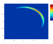
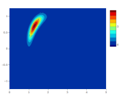
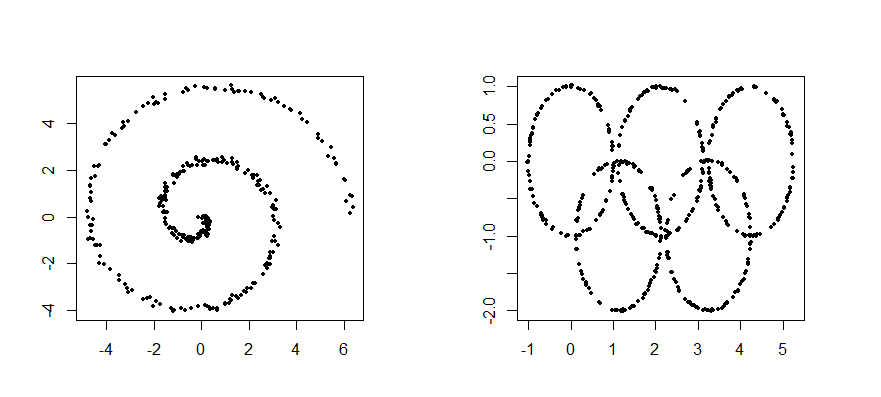
We clarify the problem using two toy examples - the noised spiral and Olympic rings - shown in Figure 1. Both are examples of d=2𝑑2d=2 dimensional data concentrated near a one dimensional curve(s).
Refer to caption
Figure 1: Scatter plot of 300 points from noised spiral (left panel), and 500500500 points from Olympic rings (right panel)

These are common toy examples from the literature on nonlinear dimensionality reduction and manifold learning (Lee and Verleysen, (2007)). We use them as motivation, since even in these simple cases problems arise for usual Gaussian kernels due to their intrinsic linear structure. In general for real world datasets, we will have limited prior knowledge about the support of the data, but in general no reason to suspect that it should be close to linear even locally. Indeed, in application areas ranging from imaging to signal processing to astrophysics, there is often strong reason to suggest substantial curvature in the data.
Refer to caption
Refer to caption
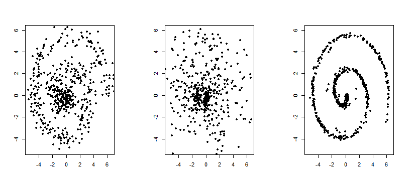
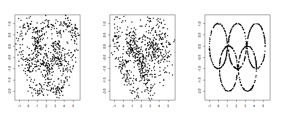
Figure 2: Scatter plot of sample points from predictive densities obtained by KDE (left), DP mixture of Gaussian (middle) and Fisher-Gaussian kernel mixture (right). The first and second rows correspond to the left and right panels from Figure 1

Figure 2 shows results from estimating the density of the data shown in Figure 1 using frequentist kernel density estimation (KDE, see, e.g., Silverman, (1986)) implemented in the ‘ks’ R-package, a Bayesian nonparametric approach relying on Dirichlet process mixtures (DPM, see, e.g., MacEachern and Müller, (1998)) of Gaussian kernels implemented in the ‘dirichletprocess’ R-package, and our proposed approach, which uses (1) within a Bayesian inference approach incorporating a novel class of kernels that accommodate curvature. For easy visualization, we plot new samples from the estimated density in each case. It is clear that the KDE and DPM of Gaussian methods fail to accurately estimate the density. This is due in large part to the fact that the multivariate Gaussian kernel has elliptical contours about a line or plane, leading to challenges in accurately locally approximating the densities of the data shown in Figure 1. The Gaussian kernel provides an accurate local approximation only in a very small region, and hence one needs many kernels and a correspondingly large sample size n𝑛n for good performance.

A natural question is whether this problem can be solved with the various alternative kernels that have been proposed in the literature. In the multivariate case, the most popular extensions have been to inflate the tails using multivariate-t kernels (McLachlan and Peel, (1998), Lee and McLachlan, (2016)) and/or to generalize the Gaussian distribution to allow skewness (Azzalini and Dalla Valle, (1996), Arellano-Valle and Azzalini, (2009)). Motivated by the problem of more robust clustering, there are also methods available for nonparametrically estimating the kernels subject to unimodality (Rodríguez and Walker, (2014)) and log concavity (Hu et al., (2016)) restrictions. Also to improve robustness of clustering, one can use a mixture of mixtures model employing multiple kernels having similar location parameters to characterize the data within a cluster (Malsiner-Walli et al., (2017)). None of these methods address the fundamental problem we focus on, which is how to better characterize curvature in the support.

An alternative strategy would be to abandon kernel-based methods entirely in attempting to characterize the density of f𝑓f more accurately. In this regard, one could potentially use flexible non-linear latent structure models developed in the machine learning literature, ranging from Gaussian process latent variable models (GP-LVMs) (Li and Chen, (2016), Doersch, (2016)) to variational auto-encoders (VAEs) leveraging deep neural networks (Lawrence, (2005)). However, such methods are complex black boxes that fail to produce an analytic expression for the density of the data and sacrifice the simple interpretation of (1) in terms of producing data clusters that each have a known distributional form.

With this motivation, we propose to generalize the Gaussian kernel to accommodate curvature in a simple and analytically tractable manner. In particular, we develop a new class of Fisher-Gaussian (FG) kernels by generating observations from a von Mises-Fisher density on a sphere and adding Gaussian noise. The resulting FG distribution has an analytic form, and includes a curvature parameter, in addition to location and scale parameters. Using this kernel, we propose FG mixture models and implement these models within a Bayesian framework using Markov chain Monte Carlo (MCMC).

Section 2 derives the FG class of kernels and studies basic distributional properties and representations. Section 3 includes these kernels within a Bayesian mixture model, and develops a straightforward MCMC algorithm for posterior computation. Section 4 studies asymptotic properties. Section 5 contains a simulation study. Section 6 applies the methods to several datasets, and Section 7 contains a discussion. Proofs are included in the Appendix.

2 The Fisher-Gaussian kernel

Suppose the observed data, 𝐱1,,𝐱nsubscript𝐱1subscript𝐱𝑛{\bf x}_{1},\ldots,{\bf x}_{n}, are supported around a sphere with center 𝐜𝐜{\bf c} and radius r𝑟r. Due to noise we do not observe points exactly on the sphere. Therefore we model the data as

𝐱i=𝐜+r𝐲i+ϵiwhere ϵiN(𝟎,σ2I),formulae-sequencesubscript𝐱𝑖𝐜𝑟subscript𝐲𝑖subscriptbold-italic-ϵ𝑖similar-towhere subscriptbold-italic-ϵ𝑖𝑁0superscript𝜎2𝐼{\bf x}_{i}={\bf c}+r{\bf y}_{i}+\boldsymbol{\epsilon}_{i}\quad\mbox{where }~{}~{}\boldsymbol{\epsilon}_{i}\sim N\left({\bf 0},\sigma^{2}I\right), (2)

for some unknown noise variance σ2>0superscript𝜎20\sigma^{2}>0. Here 𝐜+r𝐲i𝐜𝑟subscript𝐲𝑖{\bf c}+r{\bf y}_{i} is the part of 𝐱isubscript𝐱𝑖{\bf x}_{i} supported exactly on the sphere with center 𝐜𝐜{\bf c} and radius r𝑟r, and ϵisubscriptbold-italic-ϵ𝑖\boldsymbol{\epsilon}_{i} is a random noise. The random variable 𝐲i=(𝐱i𝐜ϵi)/rsubscript𝐲𝑖subscript𝐱𝑖𝐜subscriptbold-italic-ϵ𝑖𝑟{\bf y}_{i}=\left({\bf x}_{i}-{\bf c}-\boldsymbol{\epsilon}_{i}\right)/r has support on the unit sphere, and is assumed to follow a von-Mises Fisher density as 𝐲ifvMF(𝝁,τ){\bf y}_{i}\sim f_{\mathrm{vMF}}\left(\cdot\mid\boldsymbol{\mu},\tau\right), where 𝝁𝝁\boldsymbol{\mu} is the mean direction, and τ𝜏\tau is a concentration parameter. Higher values of τ𝜏\tau indicate higher concentration of the distribution around 𝝁𝝁\boldsymbol{\mu}. Thus the density of 𝐱𝐱{\bf x} is

f(𝐱)𝑓𝐱\displaystyle f({\bf x}) =d1rdfvMF{1r(𝐱𝐜ϵ)𝝁,τ}ϕσ2(ϵ)𝑑ϵabsentsubscriptsuperscript𝑑1superscript𝑟𝑑subscript𝑓vMFconditional-set1𝑟𝐱𝐜bold-italic-ϵ𝝁𝜏subscriptitalic-ϕsuperscript𝜎2bold-italic-ϵdifferential-dbold-italic-ϵ\displaystyle=\int_{\mathbb{R}^{d}}\frac{1}{r^{d}}f_{\mathrm{vMF}}\left\{\frac{1}{r}\left({\bf x}-{\bf c}-\boldsymbol{\epsilon}\right)\mid\boldsymbol{\mu},\tau\right\}\phi_{\sigma^{2}}\left(\boldsymbol{\epsilon}\right)d\boldsymbol{\epsilon}
=d1rdfvMF{1r(𝐳𝐜)𝝁,τ}ϕσ2(𝐱𝐳)𝑑𝐳,absentsubscriptsuperscript𝑑1superscript𝑟𝑑subscript𝑓vMFconditional-set1𝑟𝐳𝐜𝝁𝜏subscriptitalic-ϕsuperscript𝜎2𝐱𝐳differential-d𝐳\displaystyle\hskip 108.405pt=\int_{\mathbb{R}^{d}}\frac{1}{r^{d}}f_{\mathrm{vMF}}\left\{\frac{1}{r}\left({\bf z}-{\bf c}\right)\mid\boldsymbol{\mu},\tau\right\}\phi_{\sigma^{2}}\left({\bf x}-{\bf z}\right)d\boldsymbol{{\bf z}}, (3)

where ϕσ2()subscriptitalic-ϕsuperscript𝜎2\phi_{\sigma^{2}}(\cdot) is the multivariate normal density with mean 𝟎0{\bf 0} and variance σ2Isuperscript𝜎2𝐼\sigma^{2}I. We refer to (3) as the Fisher-Gaussian (FG) density.

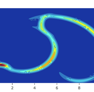
As the definition suggests, the FG density is essentially a Gaussian density concentrated near the circumference of a sphere. The kernel depends on five parameters: 𝐜𝐜{\bf c} and r𝑟r: the center and radius of the sphere along which the kernel is distributed; 𝝁𝝁\boldsymbol{\mu} and τ𝜏\tau: the location on the sphere around which the density has highest concentration and the precision along the sphere; and σ2superscript𝜎2\sigma^{2} controls how far from the sphere data points concentrate. Figure 3 (a)–(b) demonstrate the effect of the different parameters of the kernel. Throughout this paper, we denote the FG kernel as FGσ(𝝆)\mathrm{FG}_{\sigma}\left(\cdot\mid\boldsymbol{\rho}\right) where 𝝆=(𝐜,r,𝝁,τ)𝝆𝐜𝑟𝝁𝜏\boldsymbol{\rho}=\left({\bf c},r,\boldsymbol{\mu},\tau\right).

Refer to caption
Refer to caption
Refer to caption
Figure 3: Fisher-Gaussian kernel for different parameters (a) (left) 𝝁=(1/2,1/2)𝝁1212\boldsymbol{\mu}=\left(1/\sqrt{2},1/\sqrt{2}\right), τ=3𝜏3\tau=3, σ2=.001superscript𝜎2.001\sigma^{2}=.001, 𝐜=𝟎𝐜0{\bf c}={\bf 0}, r=1𝑟1r=1; (b) (middle) 𝝁=(1/2,1/2)𝝁1212\boldsymbol{\mu}=\left(-1/\sqrt{2},1/\sqrt{2}\right), τ=10𝜏10\tau=10, σ2=.01superscript𝜎2.01\sigma^{2}=.01, 𝐜=(2,0)𝐜20{\bf c}=(2,0), r=1𝑟1r=1; (c) (right) A typical example of FG-kernel mixture density.

The FG-kernel has a simple analytic form which makes it theoretically tractable, and easily applicable. By integrating out 𝐳𝐳{\bf z} in (3), the FG kernel can be expressed as follows

FGσ(𝐱𝝆)=Cd(τ)(2πσ2)(d/2)Cd(τ𝝁+r(𝐱𝐜)/σ2)exp{12σ2(𝐱𝐜2+r2)},subscriptFG𝜎conditional𝐱𝝆subscript𝐶𝑑𝜏superscript2𝜋superscript𝜎2𝑑2subscript𝐶𝑑norm𝜏𝝁𝑟𝐱𝐜superscript𝜎212superscript𝜎2superscriptnorm𝐱𝐜2superscript𝑟2\displaystyle\mathrm{FG}_{\sigma}({\bf x}\mid\boldsymbol{\rho})=\frac{C_{d}(\tau)\left(2\pi\sigma^{2}\right)^{-(d/2)}}{C_{d}\left(\|\tau\boldsymbol{\mu}+r({\bf x}-{\bf c})/\sigma^{2}\|\right)}\exp\left\{-\frac{1}{2\sigma^{2}}\left(\|{\bf x}-{\bf c}\|^{2}+r^{2}\right)\right\}, (4)

where Cd(τ)=τd/21(2π)d/2Id/211(τ)subscript𝐶𝑑𝜏superscript𝜏𝑑21superscript2𝜋𝑑2superscriptsubscript𝐼𝑑211𝜏C_{d}(\tau)=\tau^{d/2-1}(2\pi)^{-d/2}I_{d/2-1}^{-1}(\tau) and Iνsubscript𝐼𝜈I_{\nu} denotes the modified Bessel function of the first kind of order ν𝜈\nu. The following lemma proves the above claim.

Lemma 1.
  1. a.

    The density in (3) can be written as in (4).

  2. b.

    Consequently, for any given 𝝆𝝆\boldsymbol{\rho} and σ2superscript𝜎2\sigma^{2}, dFGσ(𝐱𝝆)𝑑𝐱=1subscriptsuperscript𝑑subscriptFG𝜎conditional𝐱𝝆differential-d𝐱1\int_{\mathbb{R}^{d}}\mathrm{FG}_{\sigma}\left({\bf x}\mid\boldsymbol{\rho}\right)d{\bf x}=1.

The FG kernel provides a simple and flexible generalization of the spherical Gaussian density, commonly used in multivariate density estimation, to allow “curved” densities, as illustrated in Figure 3. The curvature can be modified arbitrarily by changing the radius r𝑟r, with smaller r𝑟r providing larger curvature and larger r𝑟r providing densities close to Gaussian. Potentially, one can define a broader class of FG distributions by replacing either or both of the scale parameters τ𝜏\tau and σ2superscript𝜎2\sigma^{2} with positive semidefinite matrices, obtaining a flexible class of curved multivariate distributions. However, we leave this to future work.

3 Mixtures of Fisher-Gaussian Kernels

Although the FG distribution is useful in other settings as a simple but flexible generalization of the spherical Gaussian density, our focus is on using FG kernels in mixture models. Real data often involve nonlinear relationships among variables, and in such cases mixtures of FG kernels are expected to provide more parsimonious density approximations requiring many fewer mixture components to obtain an accurate approximation.

To make the model more parsimonious, we propose a nested modification to (1). We start by letting 𝐱i=𝐳i+ϵisubscript𝐱𝑖subscript𝐳𝑖subscriptbold-italic-ϵ𝑖{\bf x}_{i}={\bf z}_{i}+\boldsymbol{\epsilon}_{i}, as in model (2), with 𝐳isubscript𝐳𝑖{\bf z}_{i} falling exactly on a sphere. The distribution of 𝐳isubscript𝐳𝑖{\bf z}_{i} depends on parameters controlling inter (𝐜𝐜{\bf c} and r𝑟r) and intra-sphere (𝝁𝝁\boldsymbol{\mu} and τ𝜏\tau) characteristics. The parameters (𝐜,r)𝐜𝑟({\bf c},r) control the location and size of the sphere on which 𝐳isubscript𝐳𝑖{\bf z}_{i} lies, whereas (𝝁,τ)𝝁𝜏(\boldsymbol{\mu},\tau) controls the modal point and precision of the distribution of 𝐳isubscript𝐳𝑖{\bf z}_{i} on the sphere. Within a sphere, the distribution can be unimodal or multimodal. Hence, it is natural to consider a model in which one has a collection of spheres, having varying centers and radii, along with a collection of kernels on each of these spheres. Thus, we can represent the distribution of 𝐳isubscript𝐳𝑖{\bf z}_{i} as

1rsi(𝐳i𝐜si)fvMF(𝝁kisi,τkisi),\displaystyle\frac{1}{r_{s_{i}}}\left({\bf z}_{i}-{\bf c}_{s_{i}}\right)\sim f_{\mathrm{vMF}}\left(\cdot\mid\boldsymbol{\mu}_{k_{i}}^{s_{i}},\tau_{k_{i}}^{s_{i}}\right),

where sisubscript𝑠𝑖s_{i} indexes the sphere that 𝐳isubscript𝐳𝑖{\bf z}_{i} lies on, and kisubscript𝑘𝑖k_{i} indexes the kernel within the sphere from which 𝐳isubscript𝐳𝑖{\bf z}_{i} is drawn. The number of spheres, as well as vMF kernels is not known. To keep the representation simple, yet flexible, we let si{1,,}subscript𝑠𝑖1s_{i}\in\{1,\ldots,\infty\} and ki{1,,M}subscript𝑘𝑖1𝑀k_{i}\in\{1,\ldots,M\}. Under the proposed specification, we have P(si=l)=λl𝑃subscript𝑠𝑖𝑙subscript𝜆𝑙P\left(s_{i}=l\right)=\lambda_{l} for l=1,,𝑙1l=1,\ldots,\infty, and P(ki=ksi=l)=πkl𝑃subscript𝑘𝑖conditional𝑘subscript𝑠𝑖𝑙superscriptsubscript𝜋𝑘𝑙P\left(k_{i}=k\mid s_{i}=l\right)=\pi_{k}^{l} for k=1,,M𝑘1𝑀k=1,\ldots,M.

Conditionally on (si,ki)subscript𝑠𝑖subscript𝑘𝑖\left(s_{i},k_{i}\right) but marginalizing out 𝐳isubscript𝐳𝑖{\bf z}_{i}, we have

(𝐱isi=l,ki=k)FGσ(𝐜l,rl,𝝁kl,τkl),\displaystyle\left({\bf x}_{i}\mid s_{i}=l,k_{i}=k\right)\sim\mathrm{FG}_{\sigma}\left(\cdot\mid{\bf c}_{l},r_{l},\boldsymbol{\mu}_{k}^{l},\tau_{k}^{l}\right), (5)

following the FG-kernel described in (4). Further marginalizing out (si,ki)subscript𝑠𝑖subscript𝑘𝑖(s_{i},k_{i}) leads to the simple two-layer FG kernel mixture

𝐱il=1λlk=1MπklFGσ(𝐜l,rl,𝝁kl,τkl).\displaystyle{\bf x}_{i}\sim\sum_{l=1}^{\infty}\lambda_{l}\sum_{k=1}^{M}\pi_{k}^{l}\mathrm{FG}_{\sigma}\left(\cdot\mid{\bf c}_{l},r_{l},\boldsymbol{\mu}_{k}^{l},\tau_{k}^{l}\right). (6)

The proposed representation of 𝐱isubscript𝐱𝑖{\bf x}_{i} provides a very flexible setup accommodating mixtures of multimodal spherical densities, and is suitable to approximate densities concentrated near an arbitrary curved support. A representative density of x𝑥x, characterized as above, is shown in Figure 3 (c).

A Bayesian model is completed with priors for the two levels of mixture weights and the kernel parameters, as described in the next subsection.

3.1 Prior Specifications

For the mixture distribution over spheres, we use a Dirichlet process prior (DP, Ferguson, (1973), Antoniak, (1974)) with concentration parameter α𝛼\alpha and base measure G0=N(𝟎,σc2I)×N+(μr,σr2)subscript𝐺0𝑁0subscriptsuperscript𝜎2𝑐𝐼subscript𝑁subscript𝜇𝑟superscriptsubscript𝜎𝑟2G_{0}=N\left({\bf 0},\sigma^{2}_{c}I\right)\times N_{+}\left(\mu_{r},\sigma_{r}^{2}\right), where σc2,μr,σr2superscriptsubscript𝜎𝑐2subscript𝜇𝑟superscriptsubscript𝜎𝑟2\sigma_{c}^{2},\mu_{r},\sigma_{r}^{2} are positive constants and N+subscript𝑁N_{+} denotes a Gaussian density truncated to (0,).0(0,\infty). The DP prior induces a stick-breaking process (Sethuraman,, 1994) on the probability weights 𝝀=(λ1,λ2,)𝝀subscript𝜆1subscript𝜆2\boldsymbol{\lambda}=\left(\lambda_{1},\lambda_{2},\ldots\right). For the lthsuperscript𝑙𝑡l^{th} sphere, the von-Mises kernel weights 𝝅l=(π1l,,πMl)superscript𝝅𝑙subscriptsuperscript𝜋𝑙1subscriptsuperscript𝜋𝑙𝑀\boldsymbol{\pi}^{l}=\left(\pi^{l}_{1},\ldots,\pi^{l}_{M}\right) follow a Dirichlet prior with parameters a0,,a0subscript𝑎0subscript𝑎0a_{0},\ldots,a_{0} for some fixed constant a0subscript𝑎0a_{0}. For each sphere and each kernel, the parameters of the von-Mises Fisher density, (𝝁ml,τml)subscriptsuperscript𝝁𝑙𝑚subscriptsuperscript𝜏𝑙𝑚\left(\boldsymbol{\mu}^{l}_{m},\tau^{l}_{m}\right), are assigned the conjugate prior proposed in Nuñez Antonio and Gutiérrez-Peña, (2005),

p(𝝁,τ){τd/21Id/21(τ)}aexp(bτ𝝁0𝝁),proportional-to𝑝𝝁𝜏superscriptsuperscript𝜏𝑑21subscript𝐼𝑑21𝜏𝑎𝑏𝜏superscriptsubscript𝝁0𝝁p\left(\boldsymbol{\mu},\tau\right)\propto\left\{\frac{\tau^{d/2-1}}{I_{d/2-1}(\tau)}\right\}^{a}\exp\left(b\tau\boldsymbol{\mu}_{0}^{\prime}\boldsymbol{\mu}\right),

with hyper-parameters 𝝁0subscript𝝁0\boldsymbol{\mu}_{0}, a𝑎a and b𝑏b for some a>b>0𝑎𝑏0a>b>0. Given τ𝜏\tau, the marginal density of 𝝁𝝁\boldsymbol{\mu} follows a von-Mises Fisher density. However, the marginal density of τ𝜏\tau does not have a standard form. The variance of measurement error σ2superscript𝜎2\sigma^{2} is assigned an inverse-gamma prior with parameters aσ,bσ>0subscript𝑎𝜎subscript𝑏𝜎0a_{\sigma},b_{\sigma}>0, where aσsubscript𝑎𝜎a_{\sigma} and bσsubscript𝑏𝜎b_{\sigma} are constants. The choices of the hyperparameters are discussed in Section 5.

3.2 Posterior Computation

Throughout this section we use the following conventions: (i) The sphere and kernel indicators of the ithsuperscript𝑖𝑡i^{th} observation are denoted by sisubscript𝑠𝑖s_{i} and kisubscript𝑘𝑖k_{i}, respectively, and the sphere and kernel indices are denoted by l𝑙l and k𝑘k, l=1,2,𝑙12l=1,2,\ldots, k=1,,M𝑘1𝑀k=1,\ldots,M; (ii) The number of observations in the lthsuperscript𝑙𝑡l^{th} sphere is denoted by nlsuperscript𝑛𝑙n^{l}, and that in the kthsuperscript𝑘𝑡k^{th} kernel of the lthsuperscript𝑙𝑡l^{th} sphere is indicated by nklsubscriptsuperscript𝑛𝑙𝑘n^{l}_{k}; (iii) We let 𝝆kl=(𝐜l,rl,𝝁kl,τkl)superscriptsubscript𝝆𝑘𝑙subscript𝐜𝑙subscript𝑟𝑙superscriptsubscript𝝁𝑘𝑙superscriptsubscript𝜏𝑘𝑙\boldsymbol{\rho}_{k}^{l}=\left({\bf c}_{l},r_{l},\boldsymbol{\mu}_{k}^{l},\tau_{k}^{l}\right) denote the parameters of the kthsuperscript𝑘𝑡k^{th} kernel on the lthsuperscript𝑙𝑡l^{th} sphere.

We develop a Metropolis within Gibbs sampler using the characterization of the density in (3). The sampler is straightforward to implement, involving the following simple updating steps from standard distributions and no need for algorithm tuning.

Step 1

Updates on sphere labels. We follow Neal, (2000, Algorithm 8) to update the sphere labels, s1,,snsubscript𝑠1subscript𝑠𝑛s_{1},\ldots,s_{n}. Excluding the ithsuperscript𝑖𝑡i^{th} observation, suppose there are L𝐿L spheres represented in the data having parameters 𝝆klsuperscriptsubscript𝝆𝑘𝑙\boldsymbol{\rho}_{k}^{l}, πklsuperscriptsubscript𝜋𝑘𝑙\pi_{k}^{l} and σ2superscript𝜎2\sigma^{2} for l=1,,L𝑙1𝐿l=1,\ldots,L and k=1,,M𝑘1𝑀k=1,\ldots,M. Fix a number J𝐽J, and create J𝐽J additional empty sphere labels, L+1,,L+J𝐿1𝐿𝐽L+1,\ldots,L+J. If the ithsuperscript𝑖𝑡i^{th} observation was the only data point allocated to sphere Lsuperscript𝐿L^{\prime} in the last iteration, then attach the corresponding 𝝆kLsuperscriptsubscript𝝆𝑘superscript𝐿\boldsymbol{\rho}_{k}^{L^{\prime}} and πkLsuperscriptsubscript𝜋𝑘superscript𝐿\pi_{k}^{L^{\prime}} to the first empty sphere label, and associate the remaining empty sphere labels with values of 𝝆klsuperscriptsubscript𝝆𝑘𝑙\boldsymbol{\rho}_{k}^{l} and πklsuperscriptsubscript𝜋𝑘𝑙\pi_{k}^{l} generated randomly from the base distribution. We draw a new value of sisubscript𝑠𝑖s_{i} with

P(si=l){nilk=1MπklFGσ(𝐱i𝝆kl)for l=1,,L,αJ1k=1MπklFGσ(𝐱i𝝆kl)for l=L+1,,L+J,proportional-to𝑃subscript𝑠𝑖𝑙casessuperscriptsubscript𝑛𝑖𝑙superscriptsubscript𝑘1𝑀superscriptsubscript𝜋𝑘𝑙subscriptFG𝜎conditionalsubscript𝐱𝑖superscriptsubscript𝝆𝑘𝑙for l=1,,L𝛼superscript𝐽1superscriptsubscript𝑘1𝑀superscriptsubscript𝜋𝑘𝑙subscriptFG𝜎conditionalsubscript𝐱𝑖superscriptsubscript𝝆𝑘𝑙for l=L+1,,L+JP(s_{i}=l)\propto\begin{cases}n_{-i}^{l}\sum_{k=1}^{M}\pi_{k}^{l}\mathrm{FG}_{\sigma}\left({\bf x}_{i}\mid\boldsymbol{\rho}_{k}^{l}\right)&\mbox{for $l=1,\ldots,L$},\\ \alpha J^{-1}\sum_{k=1}^{M}\pi_{k}^{l}\mathrm{FG}_{\sigma}\left({\bf x}_{i}\mid\boldsymbol{\rho}_{k}^{l}\right)&\mbox{for $l=L+1,\ldots,L+J$},\end{cases} (7)

where nil=ji1(sj=l)superscriptsubscript𝑛𝑖𝑙subscript𝑗𝑖1subscript𝑠𝑗𝑙n_{-i}^{l}=\sum_{j\neq i}1\left(s_{j}=l\right) and FGσ(𝐱i𝝆)subscriptFG𝜎conditionalsubscript𝐱𝑖𝝆\mathrm{FG}_{\sigma}\left({\bf x}_{i}\mid\boldsymbol{\rho}\right) is as given in (4).

Step 2

Conditional posteriors of centers and radii. The conditional posterior of the center of the lthsuperscript𝑙𝑡l^{th} sphere 𝐜lsubscript𝐜𝑙{\bf c}_{l} follows a Gaussian density with location parameter 𝝁clsuperscriptsubscript𝝁conditional𝑐𝑙\boldsymbol{\mu}_{c\mid\cdot}^{l} and scale parameter σcl2Isubscriptsuperscript𝜎𝑙2conditional𝑐𝐼\sigma^{l~{}2}_{c\mid\cdot}I, where

𝝁cl=σc×{1σ2i=1nI(si=l)(𝐱irl𝐲i)}andσcl2=(nlσ2+1σc2)1.superscriptsubscript𝝁conditional𝑐𝑙subscript𝜎conditional𝑐1superscript𝜎2superscriptsubscript𝑖1𝑛𝐼subscript𝑠𝑖𝑙subscript𝐱𝑖subscript𝑟𝑙subscript𝐲𝑖andsubscriptsuperscript𝜎𝑙2conditional𝑐superscriptsuperscript𝑛𝑙superscript𝜎21superscriptsubscript𝜎𝑐21\boldsymbol{\mu}_{c\mid\cdot}^{l}=\sigma_{c\mid\cdot}\times\left\{\frac{1}{\sigma^{2}}\sum_{i=1}^{n}I\left(s_{i}=l\right)\left({\bf x}_{i}-r_{l}{\bf y}_{i}\right)\right\}~{}~{}\mbox{and}~{}~{}\sigma^{l~{}2}_{c\mid\cdot}=\left(\frac{n^{l}}{\sigma^{2}}+\frac{1}{\sigma_{c}^{2}}\right)^{-1}.

Similarly, the conditional posterior of the radius of the lthsuperscript𝑙𝑡l^{th} sphere rlsubscript𝑟𝑙r_{l} follows a positive Gaussian density with location parameter μrlsuperscriptsubscript𝜇conditional𝑟𝑙\mu_{r\mid\cdot}^{l} and scale parameter σrl2subscriptsuperscript𝜎𝑙2conditional𝑟\sigma^{l~{}2}_{r\mid\cdot},

μrl=σr|×{μrσr2+1σ2i=1nI(si=l)𝐲i(𝐱i𝐜l)}andσrl2=(nlσ2+1σr2)1.superscriptsubscript𝜇conditional𝑟𝑙subscript𝜎conditional𝑟subscript𝜇𝑟subscriptsuperscript𝜎2𝑟1superscript𝜎2superscriptsubscript𝑖1𝑛𝐼subscript𝑠𝑖𝑙superscriptsubscript𝐲𝑖subscript𝐱𝑖subscript𝐜𝑙andsubscriptsuperscript𝜎𝑙2conditional𝑟superscriptsuperscript𝑛𝑙superscript𝜎21superscriptsubscript𝜎𝑟21\mu_{r\mid\cdot}^{l}=\sigma_{r|\cdot}\times\left\{\frac{\mu_{r}}{\sigma^{2}_{r}}+\frac{1}{\sigma^{2}}\sum_{i=1}^{n}I\left(s_{i}=l\right){\bf y}_{i}^{\prime}\left({\bf x}_{i}-{\bf c}_{l}\right)\right\}~{}~{}\mbox{and}~{}~{}\sigma^{l~{}2}_{r\mid\cdot}=\left(\frac{n^{l}}{\sigma^{2}}+\frac{1}{\sigma_{r}^{2}}\right)^{-1}.

Step 3

Updates on von-Mises Fisher kernel allocations and weights. We first update the kernel allocation kisubscript𝑘𝑖k_{i}, for i=1,,n𝑖1𝑛i=1,\ldots,n, according to

P(ki=ksi=l,𝐲i,𝝁,τ)=πklFGσ(𝐱i𝐜l,rl,𝝁kl,τkl)m=1MπmlFGσ(𝐱i𝐜l,rl,𝝁ml,τml).P(k_{i}=k\mid s_{i}=l,{\bf y}_{i},\boldsymbol{\mu},\tau)=\frac{\pi_{k}^{l}~{}\mathrm{FG}_{\sigma}\left({\bf x}_{i}\mid{\bf c}_{l},r_{l},\boldsymbol{\mu}^{l}_{k},\tau^{l}_{k}\right)}{\sum_{m=1}^{M}\pi_{m}^{l}~{}\mathrm{FG}_{\sigma}\left({\bf x}_{i}\mid{\bf c}_{l},r_{l},\boldsymbol{\mu}^{l}_{m},\tau^{l}_{m}\right)}.

Then, the posterior distribution of (π1l,,πMl)superscriptsubscript𝜋1𝑙superscriptsubscript𝜋𝑀𝑙\left(\pi_{1}^{l},\ldots,\pi_{M}^{l}\right) is Dirichlet with parameters a0+n1l,,a0+nMlsubscript𝑎0subscriptsuperscript𝑛𝑙1subscript𝑎0subscriptsuperscript𝑛𝑙𝑀a_{0}+n^{l}_{1},\ldots,a_{0}+n^{l}_{M}.

Step 4

Update on spherical coordinates. The latent spherical location, 𝐲isubscript𝐲𝑖{\bf y}_{i}, corresponding to the ithsuperscript𝑖𝑡i^{th} observation 𝐱isubscript𝐱𝑖{\bf x}_{i}, is updated from its conditional posterior density, which is a von-Mises Fisher density with parameters 𝝁ysubscript𝝁conditional𝑦\boldsymbol{\mu}_{y\mid\cdot} and τysubscript𝜏conditional𝑦\tau_{y\mid\cdot}, where

𝝁y=τy1{rsiσ2(𝐱i𝐜si)+τkisi𝝁kisi}andτy=rsiσ2(𝐱i𝐜si)+τkisi𝝁kisi.formulae-sequencesubscript𝝁conditional𝑦superscriptsubscript𝜏conditional𝑦1subscript𝑟subscript𝑠𝑖superscript𝜎2subscript𝐱𝑖subscript𝐜subscript𝑠𝑖superscriptsubscript𝜏subscript𝑘𝑖subscript𝑠𝑖superscriptsubscript𝝁subscript𝑘𝑖subscript𝑠𝑖andsubscript𝜏conditional𝑦normsubscript𝑟subscript𝑠𝑖superscript𝜎2subscript𝐱𝑖subscript𝐜subscript𝑠𝑖superscriptsubscript𝜏subscript𝑘𝑖subscript𝑠𝑖superscriptsubscript𝝁subscript𝑘𝑖subscript𝑠𝑖\boldsymbol{\mu}_{y\mid\cdot}=\tau_{y\mid\cdot}^{-1}\left\{\frac{r_{s_{i}}}{\sigma^{2}}\left({\bf x}_{i}-{\bf c}_{s_{i}}\right)+\tau_{k_{i}}^{s_{i}}\boldsymbol{\mu}_{k_{i}}^{s_{i}}\right\}\quad\mbox{and}\quad\tau_{y\mid\cdot}=\left\|\frac{r_{s_{i}}}{\sigma^{2}}\left({\bf x}_{i}-{\bf c}_{s_{i}}\right)+\tau_{k_{i}}^{s_{i}}\boldsymbol{\mu}_{k_{i}}^{s_{i}}\right\|.

Step 5

Update on σ2superscript𝜎2\sigma^{2}. The inverse-gamma prior of σ2superscript𝜎2\sigma^{2} is conjugate yielding an inverse-gamma posterior with parameters aσsubscript𝑎conditional𝜎a_{\sigma\mid\cdot} and bσsubscript𝑏conditional𝜎b_{\sigma\mid\cdot} where

aσ=aσ+nd2andbσ=bσ+12i=1n(𝐱i𝐜sirsi𝐲i)(𝐱i𝐜sirsi𝐲i).formulae-sequencesubscript𝑎conditional𝜎subscript𝑎𝜎𝑛𝑑2andsubscript𝑏conditional𝜎subscript𝑏𝜎12superscriptsubscript𝑖1𝑛superscriptsubscript𝐱𝑖subscript𝐜subscript𝑠𝑖subscript𝑟subscript𝑠𝑖subscript𝐲𝑖subscript𝐱𝑖subscript𝐜subscript𝑠𝑖subscript𝑟subscript𝑠𝑖subscript𝐲𝑖a_{\sigma\mid\cdot}=a_{\sigma}+\displaystyle\frac{nd}{2}\quad\mbox{and}\quad b_{\sigma\mid\cdot}=b_{\sigma}+\displaystyle\frac{1}{2}\displaystyle\sum_{i=1}^{n}\left({\bf x}_{i}-{\bf c}_{s_{i}}-r_{s_{i}}{\bf y}_{i}\right)^{\prime}\left({\bf x}_{i}-{\bf c}_{s_{i}}-r_{s_{i}}{\bf y}_{i}\right).

Step 6

Update on parameters of von-Mises Fisher distributions. Finally, for each sphere, l𝑙l, and each kernel, k𝑘k, the vMF parameters are updated based on the observations associated with that sphere-kernel combination. The conditional prior on 𝝁klsubscriptsuperscript𝝁𝑙𝑘\boldsymbol{\mu}^{l}_{k} given τklsubscriptsuperscript𝜏𝑙𝑘\tau^{l}_{k} is von-Mises Fisher, and is conjugate yielding a vMF posterior with parameters 𝝁0subscript𝝁conditional0\boldsymbol{\mu}_{0\mid\cdot} and τμsubscript𝜏conditional𝜇\tau_{\mu\mid\cdot} where

𝝁0=τμ1𝐰klandτμ=𝐰kl,with𝐰kl=τkl{b𝝁0+i=1nI(si=l,ki=k)𝐲i}.formulae-sequencesubscript𝝁conditional0superscriptsubscript𝜏conditional𝜇1superscriptsubscript𝐰𝑘𝑙andsubscript𝜏conditional𝜇normsubscriptsuperscript𝐰𝑙𝑘withsubscriptsuperscript𝐰𝑙𝑘superscriptsubscript𝜏𝑘𝑙𝑏subscript𝝁0superscriptsubscript𝑖1𝑛𝐼formulae-sequencesubscript𝑠𝑖𝑙subscript𝑘𝑖𝑘subscript𝐲𝑖\boldsymbol{\mu}_{0\mid\cdot}=\tau_{\mu\mid\cdot}^{-1}{\bf w}_{k}^{l}~{}~{}\mbox{and}~{}\tau_{\mu\mid\cdot}=\left\|{\bf w}^{l}_{k}\right\|,~{}~{}\mbox{with}~{}~{}{\bf w}^{l}_{k}=\tau_{k}^{l}\left\{b\boldsymbol{\mu}_{0}+\sum_{i=1}^{n}I\left(s_{i}=l,k_{i}=k\right){\bf y}_{i}\right\}.

The conditional posterior of τklsubscriptsuperscript𝜏𝑙𝑘\tau^{l}_{k} given other parameters is

pkl(τ){τd/21Id/21(τ)}a+nklexp[τ{b𝝁0+iI(si=l,ki=k)𝐲i}𝝁kl].proportional-tosuperscriptsubscript𝑝𝑘𝑙conditional𝜏superscriptsuperscript𝜏𝑑21subscript𝐼𝑑21𝜏𝑎subscriptsuperscript𝑛𝑙𝑘𝜏superscript𝑏subscript𝝁0subscript𝑖𝐼formulae-sequencesubscript𝑠𝑖𝑙subscript𝑘𝑖𝑘subscript𝐲𝑖superscriptsubscript𝝁𝑘𝑙p_{k}^{l}\left(\tau\mid\cdot\right)\propto\left\{\frac{\tau^{d/2-1}}{I_{d/2-1}(\tau)}\right\}^{a+n^{l}_{k}}\exp\left[\tau\left\{b\boldsymbol{\mu}_{0}+\sum_{i}I\left(s_{i}=l,k_{i}=k\right){\bf y}_{i}\right\}^{\prime}\boldsymbol{\mu}_{k}^{l}\right].

We apply a Metropolis-Hastings algorithm with an independence sampler, considering a Gamma(2,ukl)Gamma2subscriptsuperscript𝑢𝑙𝑘\mathrm{Gamma}\left(2,u^{l}_{k}\right) proposal distribution. The details on choice of uklsubscriptsuperscript𝑢𝑙𝑘u^{l}_{k} are given in Section 5.

4 Asymptotic Properties

In this section, we show the Kullback-Leibler (KL) support property of the proposed prior, which implies weak posterior consistency (see Schwartz, (1965)).

Let f0subscript𝑓0f_{0} be the true density function. Under the mixture of FG-kernel approach, the proposed density function f𝑓f is described in (6). For simplicity we show the KL property holds under a restrictive version of our model in which the same vMF parameters are re-used across the different spheres. Under this assumption, we have

fP,σ(𝐱)𝐳ϕσ2(𝐱𝐳){1rdj=1MπjfvMF(𝐳𝐜r|𝐜,r,𝝁j,τj)dP}d𝐳,\displaystyle f_{P,\sigma}({\bf x})\coloneqq\int_{\bf z}\phi_{\sigma^{2}}({\bf x}-{\bf z})\left\{\int\frac{1}{r^{d}}\sum_{j=1}^{M}\pi_{j}f_{\mathrm{vMF}}\left(\frac{{\bf z}-{\bf c}}{r}\,\middle|\,{\bf c},r,\boldsymbol{\mu}_{j},\tau_{j}\right)dP\right\}d{\bf z}, (8)

where the mixing distribution of (𝐜,r,𝝅)𝐜𝑟𝝅({\bf c},r,\boldsymbol{\pi}), P𝑃P, follows a DP prior with base measure N(0,σc2Id)×Nδ(μr,σr2)×Dir(p,,p)𝑁0subscriptsuperscript𝜎2𝑐subscript𝐼𝑑subscript𝑁𝛿subscript𝜇𝑟subscriptsuperscript𝜎2𝑟Dir𝑝𝑝N\left(0,\sigma^{2}_{c}I_{d}\right)\times N_{\delta}\left(\mu_{r},\sigma^{2}_{r}\right)\times\mathrm{Dir}\left(p,\ldots,p\right). Here {𝝁1,,𝝁M}subscript𝝁1subscript𝝁𝑀\{\boldsymbol{\mu}_{1},\ldots,\boldsymbol{\mu}_{M}\} and {τ1,,τM}subscript𝜏1subscript𝜏𝑀\{\tau_{1},\ldots,\tau_{M}\} are prefixed quantities. The hyperparameters σc2superscriptsubscript𝜎𝑐2\sigma_{c}^{2}, μrsubscript𝜇𝑟\mu_{r}, δ𝛿\delta and σr2superscriptsubscript𝜎𝑟2\sigma_{r}^{2} are assumed to be elicited a priori.

First, we state a lemma which makes the mixture density in (6) more theoretically tractable.

Lemma 2.

For any 𝛒=(𝐜,r,𝛍,τ)𝛒𝐜𝑟𝛍𝜏\boldsymbol{\rho}=({\bf c},r,\boldsymbol{\mu},\tau) and σ𝜎\sigma, let the FG kernel be as in (4), then the following holds:

  1. a.

    For d>2𝑑2d>2, (2πσ2)d/2exp{12σ2(𝐱𝐜+r)2}FGσ(𝐱𝝆)superscript2𝜋superscript𝜎2𝑑212superscript𝜎2superscriptnorm𝐱𝐜𝑟2subscriptFG𝜎conditional𝐱𝝆\displaystyle(2\pi\sigma^{2})^{-d/2}\exp\left\{-\displaystyle\frac{1}{2\sigma^{2}}\left(\|{\bf x}-{\bf c}\|+r\right)^{2}\right\}\leq\mathrm{FG}_{\sigma}\left({\bf x}\mid\boldsymbol{\rho}\right)

    2(2πσ2)d/2exp{12σ2(𝐱𝐜r)2}.absent2superscript2𝜋superscript𝜎2𝑑212superscript𝜎2superscriptnorm𝐱𝐜𝑟2\leq 2(2\pi\sigma^{2})^{-d/2}\exp\left\{-\displaystyle\frac{1}{2\sigma^{2}}\left(\displaystyle\|{\bf x}-{\bf c}\|-r\right)^{2}\right\}.

  2. b.

    For d=2𝑑2d=2, the above inequality holds with left and right hand sides multiplied by exp(2τ)2𝜏\exp(-2\tau) and exp(2τ)2𝜏\exp(2\tau), respectively.

Let the true density be f0subscript𝑓0f_{0}, and KL(f0,f)=f0log(f0/f)𝐾𝐿subscript𝑓0𝑓subscript𝑓0subscript𝑓0𝑓KL\left(f_{0},f\right)=\int f_{0}\log\left(f_{0}/f\right) be the KL divergence between f0subscript𝑓0f_{0} and any density f𝑓f. Let the KL neighborhood of f0subscript𝑓0f_{0} of size ε𝜀\varepsilon be 𝒦ε(f0)={f:KL(f0,f)<ε}subscript𝒦𝜀subscript𝑓0conditional-set𝑓𝐾𝐿subscript𝑓0𝑓𝜀\mathcal{K}_{\varepsilon}(f_{0})=\left\{f:KL\left(f_{0},f\right)<\varepsilon\right\}. We say that f0subscript𝑓0f_{0} is in KL support of ΠΠ\Pi, written as f0KL(Π)subscript𝑓0𝐾𝐿Πf_{0}\in KL\left(\Pi\right), if Π{𝒦ε(f0)}>0Πsubscript𝒦𝜀subscript𝑓00\Pi\left\{\mathcal{K}_{\varepsilon}\left(f_{0}\right)\right\}>0, for every ε>0𝜀0\varepsilon>0.

Next we consider the assumptions under which our results hold.

  1. A.

    The true density f0(𝐱)<M0subscript𝑓0𝐱subscript𝑀0f_{0}({\bf x})<M_{0} for some constant M0>0subscript𝑀00M_{0}>0 for all 𝐱d𝐱superscript𝑑{\bf x}\in\mathbb{R}^{d}.

  2. B.

    The true density f0subscript𝑓0f_{0} satisfies: |f0(𝐱+𝐲)f0(𝐱)|L(𝐱)exp(s𝐲2)𝐲r0subscript𝑓0𝐱𝐲subscript𝑓0𝐱𝐿𝐱𝑠superscriptnorm𝐲2superscriptnorm𝐲subscript𝑟0|f_{0}({\bf x}+{\bf y})-f_{0}({\bf x})|\leq L({\bf x})\exp\left(s\|{\bf y}\|^{2}\right)\|{\bf y}\|^{r_{0}}, for any 𝐱,𝐲d𝐱𝐲superscript𝑑{\bf x},{\bf y}\in\mathbb{R}^{d}, some s,r00𝑠subscript𝑟00s,r_{0}\geq 0, and a non-negative function L𝐿L in dsuperscript𝑑\mathbb{R}^{d} such that L(𝐱)<Mf0(𝐱)𝐿𝐱superscript𝑀subscript𝑓0𝐱L({\bf x})<M^{\prime}f_{0}({\bf x}), for some large constant Msuperscript𝑀M^{\prime}.

  3. C.

    The qthsuperscript𝑞𝑡q^{th} order moments of 𝐱𝐱{\bf x} are finite, for some q>2𝑞2q>2.

  4. D.

    There exists a fixed point 𝐱0subscript𝐱0{\bf x}_{0} and some fixed δ>0𝛿0\delta>0 such that inf𝐱𝐱0<δf0(𝐱)=ϕδ>0subscriptinfimumnorm𝐱subscript𝐱0𝛿subscript𝑓0𝐱subscriptitalic-ϕ𝛿0\inf_{\|{\bf x}-{\bf x}_{0}\|<\delta}f_{0}({\bf x})=\phi_{\delta}>0.

Assumption A is common in the literature (see, for e.g., Wu and Ghosal, (2008)). Assumption B is weaker than the usual Hölder continuity with α=r0𝛼subscript𝑟0\alpha=r_{0}. For r0<1subscript𝑟01r_{0}<1, f0subscript𝑓0f_{0} satisfying assumption B belongs to a locally r0subscript𝑟0r_{0}-Hölder class with envelope L𝐿L (see Shen et al., (2013)). Assumptions C and D are weak conditions.

Theorem 1.

Suppose the true density f0subscript𝑓0f_{0} satisfies assumptions A-D, and the prior ΠΠ\Pi is as given in (8). Then Π{𝒦ε(f0)}>0Πsubscript𝒦𝜀subscript𝑓00\Pi\left\{\mathcal{K}_{\varepsilon}(f_{0})\right\}>0 for any ε>0𝜀0\varepsilon>0.

Remark 1.

In Theorem 1, we consider the mixing distribution of (𝐜,r,𝛑)𝐜𝑟𝛑({\bf c},r,\boldsymbol{\pi}) is P𝑃P, PDPsimilar-to𝑃𝐷𝑃P\sim DP, and (𝛍,τ)𝛍𝜏(\boldsymbol{\mu},\tau) varies on a fixed set. One can trivially extend Theorem 1 to the case where the mixing distribution of (𝐜,r,𝛑,𝛍1,,𝛍M,τ1,,τM)𝐜𝑟𝛑subscript𝛍1subscript𝛍𝑀subscript𝜏1subscript𝜏𝑀({\bf c},r,\boldsymbol{\pi},\boldsymbol{\mu}_{1},\cdots,\boldsymbol{\mu}_{M},\tau_{1},\cdots,\tau_{M}) is P𝑃P, if τ𝜏\tau is restricted to a compact set [0,τmax]0subscript𝜏[0,\tau_{\max}].

5 Simulation Experiments

In this section we carry out a variety of simulation experiments to validate our method. Our focus is on datasets which are concentrated near a manifold. We compare our method with frequentist kernel density estimation (KDE) and Dirichlet process mixtures of Gaussians (DPMG).

Our method: The algorithm is described in Section 3.2. We keep the choices of precision parameter α𝛼\alpha, and number of empty spheres J𝐽J fixed, and consider two choices of α/J𝛼𝐽\alpha/J, {1,2}12\{1,2\}. The number of von-Mises Fisher (vMF) kernels within each sphere is set to 5,105105,10 or 151515 based on the complexity of the data. The parameter a0subscript𝑎0a_{0} in the prior for the vMF kernel weights 𝝅𝝅\boldsymbol{\pi} is set to 111. The hyperparameters of the inverse-gamma prior of σ2superscript𝜎2\sigma^{2} are set to rate=1rate1\mathrm{rate}=1 and scale=0.01scale0.01\mathrm{scale}=0.01 to make the prior weakly informative. The hyperparameters of the centers and radii are set to σc2=1superscriptsubscript𝜎𝑐21\sigma_{c}^{2}=1, μr=1subscript𝜇𝑟1\mu_{r}=1 and σr=5subscript𝜎𝑟5\sigma_{r}=5. The 𝝁jsubscript𝝁𝑗\boldsymbol{\mu}_{j}s are given a vMF prior with parameters 𝝁0=(1/d,,1/d)subscript𝝁01𝑑1𝑑\boldsymbol{\mu}_{0}=\left(1/\sqrt{d},\ldots,1/\sqrt{d}\right) and a=1𝑎1a=1 with b=0.1𝑏0.1b=0.1. A small value of b𝑏b makes the prior less informative. For the independence sampler applied to update τmlsubscriptsuperscript𝜏𝑙𝑚\tau^{l}_{m}, we use a gamma proposal distribution with shape 222 and rate 2/τ^ml2subscriptsuperscript^𝜏𝑙𝑚2/\hat{\tau}^{l}_{m}. Here τ^mlsubscriptsuperscript^𝜏𝑙𝑚\hat{\tau}^{l}_{m} is an approximation to the maximum likelihood (ML) estimate of τmlsubscriptsuperscript𝜏𝑙𝑚\tau^{l}_{m}, τ^ml=t¯(dt¯)/(1t¯2)subscriptsuperscript^𝜏𝑙𝑚¯𝑡𝑑¯𝑡1superscript¯𝑡2\hat{\tau}^{l}_{m}=\bar{t}\left(d-\bar{t}\right)/\left(1-\bar{t}^{2}\right), where t¯=j𝐲j,ml/nml¯𝑡normsubscript𝑗subscriptsuperscript𝐲𝑙𝑗𝑚subscriptsuperscript𝑛𝑙𝑚\bar{t}=\|\sum_{j}{\bf y}^{l}_{j,m}\|/n^{l}_{m} (see Sra, (2012) for details on ML estimation of vMF parameters). Here 𝐲j,mlsuperscriptsubscript𝐲𝑗𝑚𝑙{\bf y}_{j,m}^{l} denotes the latent spherical coordinates of the jthsuperscript𝑗𝑡j^{th} observation belonging to the lthsuperscript𝑙𝑡l^{th} sphere and mthsuperscript𝑚𝑡m^{th} kernel. This proposal provides acceptance rates between 20%percent2020\%-40%percent4040\% in our experiments.

Other methods: For comparison we implement DMPG using the ‘DirichletProcessMvnormal’ function in the ‘dirichletprocess’ R-package with all default settings. Multivariate Gaussian kernels are used, with the base measure of the DP corresponding to a multivariate normal-inverse Wishart distribution and with the concentration parameter α𝛼\alpha given a gamma prior. Algorithm 8 in Neal, (2000) is used for sampling. For kernel density estimation (KDE) we use the ‘kde’ function with default settings in the ‘ks’ R-package. This corresponds to using multivariate Gaussian kernels with covariance/bandwidth matrix H𝐻H. By default ‘ks’ selects the bandwidth H𝐻H by direct plug-in methodology, as described in Wand and Jones, (1994) and Chacón and Duong, (2010) for univariate and multivariate cases, respectively. Most of the packages including ‘ks’ do not allow data of dimension greater than 6 (see, for e.g., Deng and Wickham, (2011)). Thus for cases with dimension greater than 6, we use the ‘kdevine’ package. This package estimates marginal densities using KDE, and then uses the VINE copula to obtain the multivariate joint density estimate.

We split the validation into two categories: density estimation and density-based classification. Below we briefly describe the measures used to assess performance.

(i) Histogram estimate. We generate n𝑛n samples, say 𝐳1,,𝐳nsubscript𝐳1subscript𝐳𝑛{\bf z}_{1},\ldots,{\bf z}_{n}, from the predictive distribution, n𝑛n being the training size; and choose N𝑁N points, 𝐱1,,𝐱Nsubscript𝐱1subscript𝐱𝑁{\bf x}_{1},\ldots,{\bf x}_{N}, randomly with replacement from the training data. Fix a neighborhood size δ𝛿\delta. Let Wj,δz=i=1nI(𝐳i𝐱j<δ)superscriptsubscript𝑊𝑗𝛿𝑧superscriptsubscript𝑖1𝑛𝐼normsubscript𝐳𝑖subscript𝐱𝑗𝛿W_{j,\delta}^{z}=\sum_{i=1}^{n}I(\|{\bf z}_{i}-{\bf x}_{j}\|<\delta) be the number of predictive points and Wj,δx=i=1nI(𝐱i𝐱j<δ)superscriptsubscript𝑊𝑗𝛿𝑥superscriptsubscript𝑖1𝑛𝐼normsubscript𝐱𝑖subscript𝐱𝑗𝛿W_{j,\delta}^{x}=\sum_{i=1}^{n}I(\|{\bf x}_{i}-{\bf x}_{j}\|<\delta) be the number of training points in the δ𝛿\delta-neighborhood of 𝐱jsubscript𝐱𝑗{\bf x}_{j}, j=1,,N𝑗1𝑁j=1,\ldots,N. Then the histogram estimate is the mean absolute difference MADδ=j=1N|Wj,δzWj,δx|/NsubscriptMAD𝛿superscriptsubscript𝑗1𝑁superscriptsubscript𝑊𝑗𝛿𝑧superscriptsubscript𝑊𝑗𝛿𝑥𝑁\mathrm{MAD}_{\delta}=\sum_{j=1}^{N}|W_{j,\delta}^{z}-W_{j,\delta}^{x}|/N.

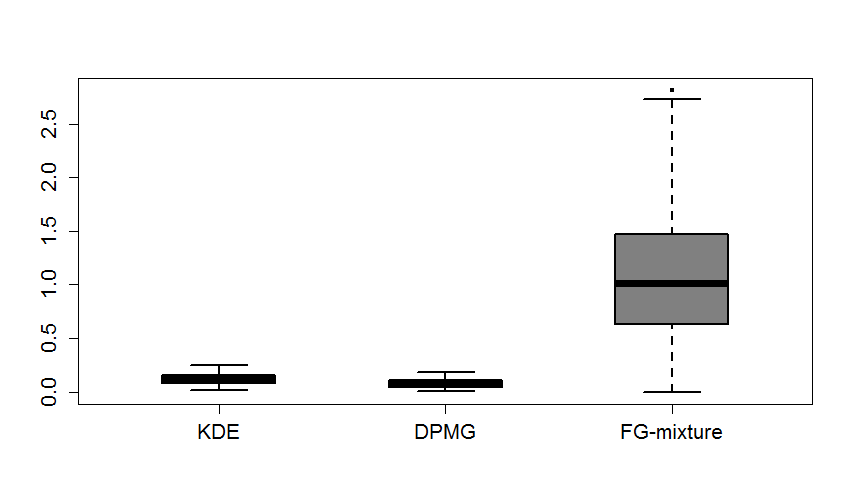
(ii) Likelihood estimate: Splitting the data into training and test sets, we estimate the density f𝑓f using the training set. We find the predictive likelihood of each test point 𝐱𝐱{\bf x}, f^(𝐱)^𝑓𝐱\hat{f}({\bf x}). Out-of-sample goodness of fit is summarized via the estimated log-likelihood, jlogf^(𝐱j)subscript𝑗^𝑓subscript𝐱𝑗\sum_{j}\log\hat{f}({\bf x}_{j}), or boxplots of f^(𝐱j)^𝑓subscript𝐱𝑗\hat{f}({\bf x}_{j}).

(iii) Classification Accuracy. Using the training data, we separately estimate the density of the features within each class. Letting f^j(𝐱)subscript^𝑓𝑗𝐱\hat{f}_{j}({\bf x}) denote the density within class j𝑗j, we assign the test data 𝐱superscript𝐱{\bf x}^{*} to the class having the highest f^j(𝐱)subscript^𝑓𝑗superscript𝐱\hat{f}_{j}\left({\bf x}^{*}\right). We then report the classification accuracy as the proportion of correct classifications in the test data.

Below we consider three density estimation examples along with a classification example.

Table 1: MADδ for different choices of δ𝛿\delta for 3 competing methods in Euler Spiral dataset
δ𝛿\delta KDE DPMG FG-mixture
0.005 0.928 0.964 0.924
0.010 2.816 3.242 1.924
0.015 4.512 5.624 2.428
0.020 5.836 7.628 2.930
0.025 6.886 9.906 3.646
0.030 7.714 11.524 4.118
0.035 8.202 13.084 4.660
Table 2: MADδ for different choices of δ𝛿\delta for 3 competing methods in ‘Olympic rings’ dataset
δ𝛿\delta KDE DPMG FG-mixture
0.025 2.102 2.242 1.646
0.050 4.256 4.782 2.688
0.075 6.014 6.858 3.526
0.100 6.838 8.392 4.118
0.125 7.316 9.906 4.738
0.150 8.072 11.086 5.350
0.175 8.850 13.122 5.278

Euler Spiral

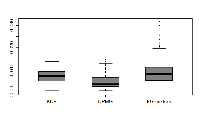
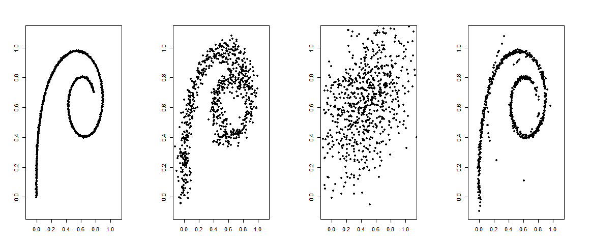
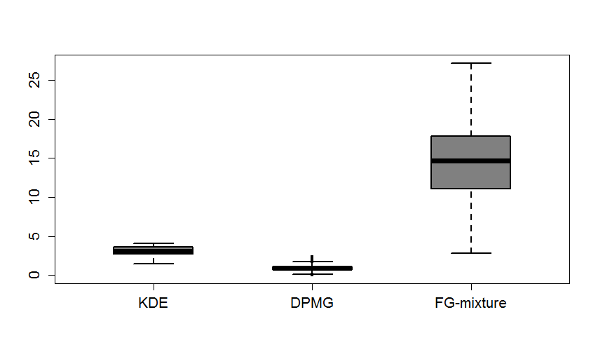
An Euler spiral is a curve whose curvature changes linearly with its curve length. We consider a sample of size 500500500 from the Euler spiral, and add a Gaussian noise of variance 0.0012Isuperscript0.0012𝐼0.001^{2}I. The mean absolute differences MADδ for N=2000𝑁2000N=2000 and different values of δ𝛿\delta are given in Table 2. Box-plots of estimated likelihoods of 300300300 test points are given in Figure 4. A Scatter plot of an Euler spiral data and that of 500500500 predictive points from each method are shown in Figure 5.
Refer to caption
Refer to caption
Figure 4: Row-wise: (i) Scatter plot of the Euler spiral dataset (first column) and 500500500 sample points from predictive densities of KDE (second column), DPMG (third column) and FG-mixture (last column). (ii) Scatter plot of the Torus dataset (first column) and 150015001500 sample points from predictive density of KDE (second column), DPMG (third column) and FG-mixture (last column).

Olympic Rings

We generate 150015001500 datapoints from 5 circles forming Olympic rings. The five circles have centers at (0,0)00(0,0), (2.125,0)2.1250(2.125,0), (4.25,0)4.250(4.25,0), (1.125,1)1.1251(1.125,-1) and (3.25,1)3.251(3.25,-1), respectively, and radii 111. We generate i×100𝑖100i\times 100 points from the ithsuperscript𝑖𝑡i^{th} circle, and add a Gaussian noise component with sd 0.010.010.01 for each component. The values of MADδ for N=2000𝑁2000N=2000 and different values of δ𝛿\delta are given in Table 2, and box-plots of estimated likelihoods are shown in Figure 5.

Torus

A torus (or torus of revolution) is a surface of revolution generated by revolving a circle in three-dimensional space about an axis coplanar with the circle. The axis of revolution does not touch the circle. We generate a dataset of n=1500𝑛1500n=1500 points on a torus using the ‘torus’ function in the ‘geozoo’ R-package. The radius of the larger circle is set to 333, that of the smaller circle is set to 111, and a Gaussian noise with variance 0.10.10.1 is added. The values of MADδ for N=1000𝑁1000N=1000 and different values of δ𝛿\delta are given in Table 4, figures of the Torus dataset and 150015001500 predictive points are shown in Figure 4, and box-plots of estimated likelihoods are in Figure 5.
Refer to caption
Refer to caption
Refer to caption
Figure 5: Box-plot of likelihood of test samples for three competing methods for Euler spiral data (left), Olympic rings data (middle) and Torus dataset (right panel)

Two-Spiral

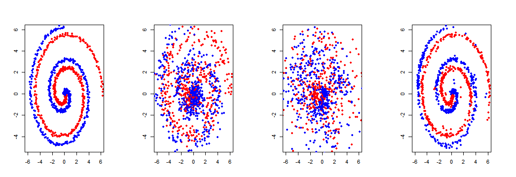
The last example is that of two spirals with varying curvature. The spirals intersect only at the center at the point of maximum curvature. As the curves move outward, the curvature of the spirals decreases simultaneously. The classification accuracies for different training test splits are given in Table 4, and the scatter plot of the actual dataset and 750750750 predictive points from each spiral are shown in Figure 6.
Refer to caption
Figure 6: Scatter plot of the ‘two spirals’ dataset (first column) and 750750750 predictive sample points from each spiral of KDE (second column), DPMG (third column) and FG-mixture (last column).
Table 3: The MADδ for different choices of δ𝛿\delta for the ‘Torus’ dataset
δ𝛿\delta KDE DPMG FG-mixture
0.1 0.121 0.096 0.117
0.2 0.626 0.552 0.625
0.3 1.255 1.381 1.204
0.4 2.127 2.653 1.982
0.5 2.829 3.991 2.611
0.6 3.703 5.754 3.121
0.7 5.515 11.071 5.340
Table 4: The accuracy for different training test split of the two-spiral dataset
Training Test Classification accuracy
size size KDE DPMG FG-mixture
50 100 0.655 0.550 0.945
100 100 0.695 0.610 0.980
150 100 0.835 0.580 0.980
200 100 0.940 0.645 0.985
250 100 0.975 0.695 0.980
300 100 0.955 0.655 0.990

The simulation results show almost uniformly better performance for the FG-mixture approach, with gains very dramatic in some cases.

6 Applications

In this section, we consider three datasets, Galaxy, Gesture Phase and Balance scale, for classification, and two datasets, User knowledge modeling and Balance scale, for density estimation. The results are given below.

Galaxy dataset

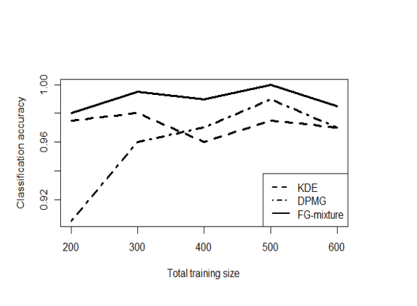
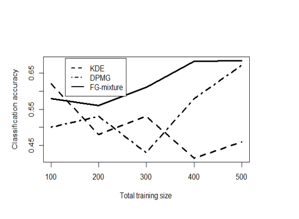
is available at https://data.galaxyzoo.org/. In the original Galaxy Zoo project (see Lintott et al., (2008) for details), volunteers classified images of Sloan Digital Sky Survey galaxies as belonging to one of six categories. We consider the first dataset (Table 2), where the galaxies are classified as spiral, elliptical or merger (i.e., uncertain). This dataset has information on 10,000 galaxies, among which 2888 are spiral and 931 are elliptical. Among these samples we consider 100100100 spiral and 100100100 elliptical galaxies at random as the test set, and vary the size of the training set. We consider 5 predictors PELsubscriptPEL\mathrm{P_{EL}}, PCWsubscriptPCW\mathrm{P_{CW}}, PEDGEsubscriptPEDGE\mathrm{P_{EDGE}}, PDKsubscriptPDK\mathrm{P_{DK}}, PMGsubscriptPMG\mathrm{P_{MG}} for classification. The classification accuracy is given in Figure 7, showing that it is improved significantly using FG mixtures.
Refer to caption
Refer to caption
Figure 7: Classification accuracies of different methods for the Galaxy (left panel) and Balance scale data (right panel). The training and test sizes for Galaxy data are (100,100)100100(100,100), (150,100)150100(150,100), (200,100)200100(200,100), (250,100)250100(250,100) and (300,100)300100(300,100); and those for Balance scale data are (50,100)50100(50,100), (100,100)100100(100,100), (150,100)150100(150,100), (200,88)20088(200,88) and (250,38)25038(250,38) from each population.

Gesture Phase dataset

is available at the UCI machine learning repository. It is composed of features extracted from 7 videos with people gesticulating, aimed at studying gesture phases. We use the processed table a1_va3, which has 323232 attributes, and 555 labels, viz., D, S, H, P, R. Among these 555 labels we discard H as it has fewer instances, and compare each pair of labels D, S, P and R. The results are shown in Table 5.

Table 5: Classification accuracies of the competing methods for the Gesture Phase data
D against P Classification Accuracy D against S Classification Accuracy
Train size * Test size * KDE DPMG FG-mixture Train size * Test size * KDE DPMG FG-mixture
50 100 ** 0.490 0.585 100 100 0.475 0.690 0.700
100 63 0.508 0.603 0.706 200 100 0.495 0.740 0.700
D against R Classification Accuracy P against S Classification Accuracy
50 100 ** 0.455 0.655 50 100 ** 0.505 0.590
100 91 0.500 0.725 0.736 100 63 0.500 0.548 0.579
P against R Classification Accuracy S against R Classification Accuracy
50 100 ** 0.530 0.585 50 100 0.495 0.475 0.550
100 63 0.516 0.627 0.635 100 91 0.532 0.595 0.611
  • *

    Train size and Test size refer to the training and test sizes of each population.

  • **

    KDE estimates of density for all the test samples are zero under both the populations.

Balance scale dataset

is generated to model psychological experimental results by Klahr and Siegler, (1978), and is obtained from the UCI repository. Each example is classified as having the balance scale tip to the right, left, or balanced. The predictors are left-weight, left-balance, right-weight and right-balance. There are 288 instances of each of left and right tipped balance scales, and we consider classification between left and right tipped balance scales. The classification accuracies are given in Figure 7.

We further use Balance scale data for density estimation. Towards that we consider training samples of various sizes from the unlabeled population, and a test data of size 100. The sum of estimated log-likelihoods of the test data is provided in Table 7.

Table 6: Sum of log-likelihoods of test samples for competing methods in Balance scale data
Training size Test size KDE DPMG FG-mixture
50 100 -645.20 -611.72 -574.93
100 100 -625.78 -571.38 -549.56
150 100 -621.60 -574.87 -550.17
200 100 -605.33 -567.37 -551.23
Table 7: Sum of log-likelihoods of test samples for competing methods in User knowledge modeling data
Training size Test size KDE DPMG FG-mixture
50 100 -230.90 -27.94 -25.69
100 100 -805.63 -713.39 -712.81
150 100 -48.30 7.36 37.21
200 58 11.88 7.46 14.30

User knowledge modeling dataset

is about the students’ knowledge status on the subject of Electrical DC Machines, and the data are obtained from the UCI repository. There are 5 attributes measuring the study time, repetition of different aspects and knowledge level, and 258 instances. The sum of estimated log likelihoods of test samples for varying training-test splits are given in Table 7

From these applications it is evident that FG mixtures clearly improve performance in both density estimation and classification, particularly in smaller samples. Also some of the improvements are quite dramatic.

7 Discussion

The main contribution of this article has been to introduce a simple generalization of the Gaussian distribution to allow the density to be concentrated near a curved support. The resulting Fisher-Gaussian distribution has a simple analytic form, and we have demonstrated that it can lead to dramatically better performance in density estimation when used in place of usual Gaussian kernels. This is particularly true when the data are concentrated near a non-linear subspace or manifold and when there are non-linear relationships among the variables being modeled, as is very commonly the case in applications. There have been many different multivariate distributions proposed in the literature, motivated largely by limitations of the multivariate Gaussian distribution in terms of symmetry and light tails, but essentially no consideration of the curved support problem. Multivariate distributions that can characterize data concentrated near a curved support tend to have a very complex form that is not analytically tractable, and hence there are considerable computational and interpretability hurdles in their implementation.

There are a number of interesting directions for future research. Natural extensions include generalizing the Fisher-Gaussian distribution to accommodate a more flexible covariance structure. One possibility is to include an arbitrary covariance in the Gaussian residual density instead of focusing on the spherical covariance case. Another is to use a more flexible generalization of the von Mises-Fisher density on the sphere; several such generalizations are available in the literature (Bingham, (1974),Kent, (1982)). We have made initial attempts along these directions and have thus far been unable to obtain an analytically tractable form for the density of the data 𝐱isubscript𝐱𝑖{\bf x}_{i} marginalizing out the coordinates on the sphere 𝐲isubscript𝐲𝑖{\bf y}_{i}. It is possible to conduct computation without such a closed form, but it will be unwieldy.

Another direction is to start with a density on a more flexible non-linear manifold than the sphere before adding Gaussian noise. Possibilities include an ellipse, quadratic surface or hyperbolic space. Unfortunately, it is not so straightforward to define tractable densities on such spaces, and it seems daunting to maintain analytic tractability in doing so. One promising direction is to start with a Gaussian on a tangent plane to a manifold and then apply the exponential map to induce a density on the target manifold. For a number of manifolds, it becomes possible to define the Jacobian and obtain a tractable form for the density on the manifold. For certain cases, it may also be possible to add Gaussian noise and marginalize out the coordinates on the manifold, as we did for the FG distribution. Otherwise, one can always rely on data augmentation algorithms for computation.

As a final fascinating direction, it will be interesting to develop theory directly justifying the use of ‘curved support’ kernels in density estimation. We have focused on showing weak posterior consistency but it would be appealing to show that a faster rate of posterior concentration can be obtained by using FG kernels instead of spherical Gaussian kernels, at least when the true density is concentrated near a non-linear manifold with sufficiently large curvature.

Acknowledgements
This research was partially supported by grant N00014-14-1-0245/N00014-16-1-2147 of the United States Office of Naval Research (ONR) and 5R01ES027498-02 of the United States National Institutes of Health (NIH).

8 Appendix

Proof of Lemma 1

Proof of part (a)..

Observe that

1rddϕσ2(𝐱𝐳)fvMF(𝐳𝐜r|𝐜,r,𝝁,τ)d𝐳\displaystyle\frac{1}{r^{d}}\int_{\mathbb{R}^{d}}\phi_{\sigma^{2}}({\bf x}-{\bf z})f_{\mathrm{vMF}}\left(\frac{{\bf z}-{\bf c}}{r}\,\middle|\,{\bf c},r,\boldsymbol{\mu},\tau\right)d{\bf z}
=1rdCd(τ)(2πσ2)d/2𝐳𝐜=rexp{12σ2𝐱𝐳2+τ(𝐳𝐜r)𝝁}𝑑𝐳absent1superscript𝑟𝑑subscript𝐶𝑑𝜏superscript2𝜋superscript𝜎2𝑑2subscriptnorm𝐳𝐜𝑟12superscript𝜎2superscriptnorm𝐱𝐳2𝜏superscript𝐳𝐜𝑟𝝁differential-d𝐳\displaystyle=\frac{1}{r^{d}}C_{d}(\tau)\left(2\pi\sigma^{2}\right)^{-d/2}\int_{\|{\bf z}-{\bf c}\|=r}\exp\left\{-\frac{1}{2\sigma^{2}}\|{\bf x}-{\bf z}\|^{2}+\tau\left(\frac{{\bf z}-{\bf c}}{r}\right)^{\prime}\boldsymbol{\mu}\right\}d{\bf z}
=1rd[Cd(τ)(2πσ2)d/2𝐳𝐜=rexp{12σ2(𝐱𝐜2+r2)\displaystyle=\frac{1}{r^{d}}\left[C_{d}(\tau)\left(2\pi\sigma^{2}\right)^{-d/2}\int_{\|{\bf z}-{\bf c}\|=r}\exp\left\{-\frac{1}{2\sigma^{2}}\left(\|{\bf x}-{\bf c}\|^{2}+r^{2}\right)\right.\right.
+(𝐳𝐜r)(τ𝝁+r(𝐱𝐜)2σ2)}d𝐳]\displaystyle\hskip 234.87749pt\left.\left.+\left(\frac{{\bf z}-{\bf c}}{r}\right)^{\prime}\left(\tau\boldsymbol{\mu}+\frac{r({\bf x}-{\bf c})}{2\sigma^{2}}\right)\right\}d{\bf z}\right]
=Cd(τ)(2πσ2)d/2𝐰=1exp{1σ2(𝐱𝐜2+r2)+𝐰(τ𝝁+r(𝐱𝐜)2σ2)}𝑑𝐰absentsubscript𝐶𝑑𝜏superscript2𝜋superscript𝜎2𝑑2subscriptnorm𝐰11superscript𝜎2superscriptnorm𝐱𝐜2superscript𝑟2superscript𝐰𝜏𝝁𝑟𝐱𝐜2superscript𝜎2differential-d𝐰\displaystyle=C_{d}(\tau)\left(2\pi\sigma^{2}\right)^{-d/2}\int_{\|{\bf w}\|=1}\exp\left\{-\frac{1}{\sigma^{2}}\left(\|{\bf x}-{\bf c}\|^{2}+r^{2}\right)+{\bf w}^{\prime}\left(\tau\boldsymbol{\mu}+\frac{r({\bf x}-{\bf c})}{2\sigma^{2}}\right)\right\}d{\bf w}
=Cd(τ)(2πσ2)(d/2)Cd(τμ+r(𝐱𝐜)/σ2)exp{12σ2(𝐱𝐜2+r2)}.absentsubscript𝐶𝑑𝜏superscript2𝜋superscript𝜎2𝑑2subscript𝐶𝑑norm𝜏𝜇𝑟𝐱𝐜superscript𝜎212superscript𝜎2superscriptnorm𝐱𝐜2superscript𝑟2\displaystyle=\frac{C_{d}(\tau)\left(2\pi\sigma^{2}\right)^{-(d/2)}}{C_{d}\left(\|\tau\mu+r({\bf x}-{\bf c})/\sigma^{2}\|\right)}\exp\left\{-\frac{1}{2\sigma^{2}}\left(\|{\bf x}-{\bf c}\|^{2}+r^{2}\right)\right\}.\hskip 144.54pt

Proof of part (b). Given 𝝆=(𝐜,r,𝝁,τ)𝝆𝐜𝑟𝝁𝜏\boldsymbol{\rho}=({\bf c},r,\boldsymbol{\mu},\tau) we can write

dFGσ(𝐱|𝝆)d𝐱=dd1rdϕσ(𝐱𝐳)fvMF(𝐳𝐜r|𝝁,τ)d𝐳d𝐱.\int_{\mathbb{R}^{d}}\mathrm{FG}_{\sigma}({\bf x}|\boldsymbol{\rho})d{\bf x}=\int_{\mathbb{R}^{d}}\int_{\mathbb{R}^{d}}\frac{1}{r^{d}}\phi_{\sigma}({\bf x}-{\bf z})f_{\mathrm{vMF}}\left(\frac{{\bf z}-{\bf c}}{r}\,\middle|\,\boldsymbol{\mu},\tau\right)d{\bf z}d{\bf x}.

Next we interchange the integrals of 𝐱𝐱{\bf x} and 𝐳𝐳{\bf z} as the integrand is non-negative and the integral is finite. After the changing the integral we get:

d1rdfvMF(𝐳𝐜r|𝝁,τ){dϕσ(𝐱𝐳)d𝐱}d𝐳=d1rdfvMF(𝐳𝐜r|𝝁,τ)d𝐳=1.\int_{\mathbb{R}^{d}}\frac{1}{r^{d}}f_{\mathrm{vMF}}\left(\frac{{\bf z}-{\bf c}}{r}\,\middle|\,\boldsymbol{\mu},\tau\right)\left\{\int_{\mathbb{R}^{d}}\phi_{\sigma}({\bf x}-{\bf z})d{\bf x}\right\}d{\bf z}=\int_{\mathbb{R}^{d}}\frac{1}{r^{d}}f_{\mathrm{vMF}}\left(\frac{{\bf z}-{\bf c}}{r}\,\middle|\,\boldsymbol{\mu},\tau\right)d{\bf z}=1.

Proof of Lemma 2

Proof.

Let r(𝐱𝐜)/σ2=𝐰𝑟𝐱𝐜superscript𝜎2𝐰r({\bf x}-{\bf c})/\sigma^{2}={\bf w}. Note that

Cd(τ)Cd(τ𝝁+𝐰)=τ𝝁+𝐰(d/21)Id/21(τ𝝁+𝐰)(τ)(d/21)Id/21(τ).subscript𝐶𝑑𝜏subscript𝐶𝑑norm𝜏𝝁𝐰superscriptnorm𝜏𝝁𝐰𝑑21subscript𝐼𝑑21𝜏𝝁𝐰superscript𝜏𝑑21subscript𝐼𝑑21𝜏\frac{C_{d}(\tau)}{C_{d}\left(\left\|\tau\boldsymbol{\mu}+{\bf w}\right\|\right)}=\frac{\|\tau\boldsymbol{\mu}+{\bf w}\|^{-(d/2-1)}I_{d/2-1}(\tau\boldsymbol{\mu}+{\bf w})}{(\tau)^{-(d/2-1)}I_{d/2-1}(\tau)}.

By (Baricz,, 2010, Equation (2.2)), for d>2𝑑2d>2,

exp{|τ𝝁+𝐰τ|}(τ𝝁+𝐰)(d/21)Id/21(τ𝝁+𝐰)(τ)(d/21)Id/21(τ)exp(|τ𝝁+𝐰τ|).norm𝜏𝝁𝐰𝜏superscript𝜏𝝁𝐰𝑑21subscript𝐼𝑑21𝜏𝝁𝐰superscript𝜏𝑑21subscript𝐼𝑑21𝜏norm𝜏𝝁𝐰𝜏\exp\left\{-\left|\|\tau\boldsymbol{\mu}+{\bf w}\|-\tau\right|\right\}\leq\frac{(\tau\boldsymbol{\mu}+{\bf w})^{-(d/2-1)}I_{d/2-1}(\tau\boldsymbol{\mu}+{\bf w})}{(\tau)^{-(d/2-1)}I_{d/2-1}(\tau)}\leq\exp\left(\left|\|\tau\boldsymbol{\mu}+{\bf w}\|-\tau\right|\right).

Next, observe that

|τ𝐰|τ𝜏norm𝐰𝜏\displaystyle\left|\tau-\|{\bf w}\|\right|-\tau |τ𝝁+𝐰τ|absentnorm𝜏𝝁𝐰𝜏\displaystyle\leq\left|\|\tau\boldsymbol{\mu}+{\bf w}\|-\tau\right| 𝐰whenτ𝝁+𝐰>τ,formulae-sequenceabsentnorm𝐰whennorm𝜏𝝁𝐰𝜏\displaystyle\leq\|{\bf w}\|\qquad\mbox{when}\quad\|\tau\boldsymbol{\mu}+{\bf w}\|>\tau,
𝐰norm𝐰\displaystyle-\|{\bf w}\| |τ𝝁+𝐰τ|absentnorm𝜏𝝁𝐰𝜏\displaystyle\leq\left|\|\tau\boldsymbol{\mu}+{\bf w}\|-\tau\right| τ|τ𝐰|whenτ𝝁+𝐰τ,formulae-sequenceabsent𝜏𝜏norm𝐰whennorm𝜏𝝁𝐰𝜏\displaystyle\leq\tau-\left|\tau-\|{\bf w}\|\right|\qquad\mbox{when}\quad\|\tau\boldsymbol{\mu}+{\bf w}\|\leq\tau,

as 𝝁=1norm𝝁1\|\boldsymbol{\mu}\|=1 and |𝐚𝐛|𝐚+𝐛𝐚+𝐛norm𝐚norm𝐛norm𝐚𝐛norm𝐚norm𝐛|\|{\bf a}\|-\|{\bf b}\||\leq\|{\bf a}+{\bf b}\|\leq\|{\bf a}\|+\|{\bf b}\|. This reduces to

𝐰norm𝐰\displaystyle-\|{\bf w}\| |τ𝝁+𝐰τ|absentnorm𝜏𝝁𝐰𝜏\displaystyle\leq\left|\|\tau\boldsymbol{\mu}+{\bf w}\|-\tau\right| 𝐰when𝐰τ<τ𝝁+𝐰formulae-sequenceabsentnorm𝐰whennorm𝐰𝜏norm𝜏𝝁𝐰\displaystyle\leq\|{\bf w}\|\qquad\mbox{when}\quad\|{\bf w}\|\leq\tau<\|\tau\boldsymbol{\mu}+{\bf w}\|
orτmax{𝐰,τ𝝁+𝐰},or𝜏norm𝐰norm𝜏𝝁𝐰\displaystyle\qquad\qquad\mbox{or}\quad\tau\geq\max\left\{\|{\bf w}\|,\|\tau\boldsymbol{\mu}+{\bf w}\|\right\},
𝐰2τnorm𝐰2𝜏\displaystyle\|{\bf w}\|-2\tau |τ𝝁+𝐰τ|absentnorm𝜏𝝁𝐰𝜏\displaystyle\leq\left|\|\tau\boldsymbol{\mu}+{\bf w}\|-\tau\right| 𝐰whenτ<min{𝐰,τ𝝁+𝐰},formulae-sequenceabsentnorm𝐰when𝜏norm𝐰norm𝜏𝝁𝐰\displaystyle\leq\|{\bf w}\|\qquad\mbox{when}\quad\tau<\min\left\{\|{\bf w}\|,\|\tau\boldsymbol{\mu}+{\bf w}\|\right\},
𝐰norm𝐰\displaystyle-\|{\bf w}\| |τ𝝁+𝐰τ|absentnorm𝜏𝝁𝐰𝜏\displaystyle\leq\left|\|\tau\boldsymbol{\mu}+{\bf w}\|-\tau\right| 2τ𝐰whenτ𝝁+𝐰τ𝐰.formulae-sequenceabsent2𝜏norm𝐰whennorm𝜏𝝁𝐰𝜏norm𝐰\displaystyle\leq 2\tau-\|{\bf w}\|\qquad\mbox{when}\quad\|\tau\boldsymbol{\mu}+{\bf w}\|\leq\tau\leq\|{\bf w}\|.

Finally, when τ<𝐰𝜏norm𝐰\tau<\|{\bf w}\| then 𝐰2τ𝐰norm𝐰2𝜏norm𝐰\|{\bf w}\|-2\tau\geq-\|{\bf w}\|, and when 2τ𝐰<𝐰2𝜏norm𝐰norm𝐰2\tau-\|{\bf w}\|<\|{\bf w}\|. Thus, 𝐰|τ𝝁+𝐰τ|𝐰norm𝐰norm𝜏𝝁𝐰𝜏norm𝐰-\|{\bf w}\|\leq\left|\|\tau\boldsymbol{\mu}+{\bf w}\|-\tau\right|\leq\|{\bf w}\| for all choices of τ𝜏\tau and 𝐰𝐰{\bf w}. The result for d>2𝑑2d>2 immediately follows by inserting the above inequality in the kernel.

For d=2𝑑2d=2, i.e., (d/21)=0𝑑210(d/2-1)=0, observe that for x0𝑥0x\geq 0, I0(x)=1π0πexp(xcosθ)𝑑θexI0(x)exsubscript𝐼0𝑥1𝜋superscriptsubscript0𝜋𝑥cos𝜃differential-d𝜃superscript𝑒𝑥subscript𝐼0𝑥superscript𝑒𝑥I_{0}(x)=\frac{1}{\pi}\int_{0}^{\pi}\exp\left(x\mathrm{cos}\theta\right)d\theta\implies e^{-x}\leq I_{0}(x)\leq e^{x}. Therefore,

exp(2τw)exp(τ𝝁+𝐰τ)2𝜏norm𝑤norm𝜏𝝁𝐰𝜏\displaystyle\exp\left(-2\tau-\|w\|\right)\leq\exp\left(-\|\tau\boldsymbol{\mu}+{\bf w}\|-\tau\right) \displaystyle\leq (τ𝝁+𝐰)(d/21)Id/21(τ𝝁+𝐰)(τ)(d/21)Id/21(τ)superscript𝜏𝝁𝐰𝑑21subscript𝐼𝑑21𝜏𝝁𝐰superscript𝜏𝑑21subscript𝐼𝑑21𝜏\displaystyle\displaystyle\frac{(\tau\boldsymbol{\mu}+{\bf w})^{-(d/2-1)}I_{d/2-1}(\tau\boldsymbol{\mu}+{\bf w})}{(\tau)^{-(d/2-1)}I_{d/2-1}(\tau)}
\displaystyle\leq exp(τ𝝁+𝐰+τ)exp(2τ+𝐰).norm𝜏𝝁𝐰𝜏2𝜏norm𝐰\displaystyle\exp\left(\|\tau\boldsymbol{\mu}+{\bf w}\|+\tau\right)\leq\exp\left(2\tau+\|{\bf w}\|\right).

This completes the proof for d=2𝑑2d=2. ∎

8.1 Proof of Theorem 1

Proof.

The proof uses ideas of similar proofs from Wu and Ghosal, (2008). The proof is done in three parts shown in the following lemma, which is same as Theorem 1 in Wu and Ghosal, (2008).

Lemma 3.

Let σ2Ssuperscript𝜎2𝑆\sigma^{2}\in S, 𝛉Θ𝛉Θ\boldsymbol{\theta}\in\Theta, P𝑃P be the mixing distribution on ΘΘ\Theta, i.e., fP,σ2()=FGσ(Θ)dP(Θ)f_{P,\sigma^{2}}(\cdot)=\int\mathrm{FG}_{\sigma}(\cdot\mid\Theta)dP(\Theta) where FGσ(Θ)\mathrm{FG}_{\sigma}(\cdot\mid\Theta) is as described in (4). Further, let (Θ)Θ\mathcal{M}\left(\Theta\right) be the space of probability measures on ΘΘ\Theta. Suppose there exists Pεsubscript𝑃𝜀P_{\varepsilon}, σε2subscriptsuperscript𝜎2𝜀\sigma^{2}_{\varepsilon}, S+𝑆superscriptS\in\mathbb{R}^{+} and 𝒲(Θ)𝒲Θ\mathcal{W}\in\mathcal{M}\left(\Theta\right), such that p(𝒲)>0𝑝𝒲0p(\mathcal{W})>0 and p(S)>0𝑝𝑆0p(S)>0, where p𝑝p denotes the prior distribution, and the followings hold:

  1. I.

    df0(𝐱)logf0(𝐱)fPε,σε2(𝐱)d𝐱<εsubscriptsuperscript𝑑subscript𝑓0𝐱subscript𝑓0𝐱subscript𝑓subscript𝑃𝜀superscriptsubscript𝜎𝜀2𝐱𝑑𝐱𝜀\displaystyle\int_{\mathbb{R}^{d}}f_{0}({\bf x})\log\displaystyle\frac{f_{0}({\bf x})}{f_{P_{\varepsilon},\sigma_{\varepsilon}^{2}}({\bf x})}d{\bf x}<\varepsilon,

  2. II.

    df0(𝐱)logfPε,σε2(𝐱)fPε,σ2(𝐱)d𝐱<εsubscriptsuperscript𝑑subscript𝑓0𝐱subscript𝑓subscript𝑃𝜀superscriptsubscript𝜎𝜀2𝐱subscript𝑓subscript𝑃𝜀superscript𝜎2𝐱𝑑𝐱𝜀\displaystyle\int_{\mathbb{R}^{d}}f_{0}({\bf x})\log\displaystyle\frac{f_{P_{\varepsilon},\sigma_{\varepsilon}^{2}}({\bf x})}{f_{P_{\varepsilon},\sigma^{2}}({\bf x})}d{\bf x}<\varepsilon for every σ2Ssuperscript𝜎2𝑆\sigma^{2}\in S,

  3. III.

    df0logfPε,σ2(𝐱)fP,σ2(𝐱)d𝐱<εsubscriptsuperscript𝑑subscript𝑓0subscript𝑓subscript𝑃𝜀superscript𝜎2𝐱subscript𝑓𝑃superscript𝜎2𝐱𝑑𝐱𝜀\displaystyle\int_{\mathbb{R}^{d}}f_{0}\log\displaystyle\frac{f_{P_{\varepsilon},\sigma^{2}}({\bf x})}{f_{P,\sigma^{2}}({\bf x})}d{\bf x}<\varepsilon for every P𝒲𝑃𝒲P\in\mathcal{W} and σ2Ssuperscript𝜎2𝑆\sigma^{2}\in S,

then f0KL(Π)subscript𝑓0𝐾𝐿Πf_{0}\in KL\left(\Pi\right), where KL(Π)𝐾𝐿ΠKL(\Pi) is as described in Section 4.

The proof is same as the proof of (Wu and Ghosal,, 2008, Theorem 1), as σ2superscript𝜎2\sigma^{2} is independent of P𝑃P.

The proof of Theorem 1 relies on showing that the above conditions hold for our proposed prior. Without loss of generality we assume that the fixed point 𝐱0subscript𝐱0{\bf x}_{0} in assumption C is 𝟎0{\bf 0}.

Showing condition (I) holds: We choose Pεsubscript𝑃𝜀P_{\varepsilon} and σε2superscriptsubscript𝜎𝜀2\sigma_{\varepsilon}^{2} as follows. For any ε>0𝜀0\varepsilon>0 we fix an mεsubscript𝑚𝜀m_{\varepsilon} such that

fε(𝐜)={tmf0(𝐜)𝐜<mε,0otherwise,subscript𝑓𝜀𝐜casessubscript𝑡𝑚subscript𝑓0𝐜norm𝐜subscript𝑚𝜀0otherwise,\displaystyle f_{\varepsilon}({\bf c})=\begin{cases}t_{m}f_{0}({\bf c})&\|{\bf c}\|<m_{\varepsilon},\\ 0&\mbox{otherwise,}\end{cases}

where tm1=𝐜<mεf0(𝐜)𝑑csuperscriptsubscript𝑡𝑚1subscriptnorm𝐜subscript𝑚𝜀subscript𝑓0𝐜differential-d𝑐t_{m}^{-1}=\int_{\|{\bf c}\|<m_{\varepsilon}}f_{0}({\bf c})dc, and r=mεη𝑟superscriptsubscript𝑚𝜀𝜂r=m_{\varepsilon}^{-\eta} for some η>0𝜂0\eta>0 with probability 1. The weight 𝝅ε=𝝅0subscript𝝅𝜀subscript𝝅0\boldsymbol{\pi}_{\varepsilon}=\boldsymbol{\pi}_{0} for any 𝝅0ΔMsubscript𝝅0subscriptΔ𝑀\boldsymbol{\pi}_{0}\in\Delta_{M}, ΔMsubscriptΔ𝑀\Delta_{M} being the M𝑀M-dimensional simplex, with probability 1. Let Fεsubscript𝐹𝜀F_{\varepsilon} be the probability measure corresponding to fεsubscript𝑓𝜀f_{\varepsilon}, then Pε=Fε×δ(mεη)subscript𝑃𝜀subscript𝐹𝜀𝛿superscriptsubscript𝑚𝜀𝜂P_{\varepsilon}=F_{\varepsilon}\times\delta\left(m_{\varepsilon}^{-\eta}\right), where δ𝛿\delta denotes the degenerate distribution. Also let σε=rε=mεηsubscript𝜎𝜀subscript𝑟𝜀superscriptsubscript𝑚𝜀𝜂\sigma_{\varepsilon}=r_{\varepsilon}=m_{\varepsilon}^{-\eta}, with probability 1. Here (mε,η)subscript𝑚𝜀𝜂(m_{\varepsilon},\eta) is such that E(𝐱2(η+1))<𝐸superscriptnorm𝐱2𝜂1E\left(\|{\bf x}\|^{2(\eta+1)}\right)<\infty (see assumption C), and mε2η>4ssuperscriptsubscript𝑚𝜀2𝜂4𝑠m_{\varepsilon}^{2\eta}>4s, where s𝑠s is as in assumption B.

Therefore, fεsubscript𝑓𝜀f_{\varepsilon} is as follows:

fε(𝐱)=𝐜<mεj=1Mπ0,jtmCd(τj)(2πσε2)(d/2)Cd(τj𝝁j+rε(𝐱𝐜)/σε2)exp{12(𝐱𝐜2σε2+1)}f0(𝐜)d𝐜.subscript𝑓𝜀𝐱subscriptnorm𝐜subscript𝑚𝜀superscriptsubscript𝑗1𝑀subscript𝜋0𝑗subscript𝑡𝑚subscript𝐶𝑑subscript𝜏𝑗superscript2𝜋superscriptsubscript𝜎𝜀2𝑑2subscript𝐶𝑑normsubscript𝜏𝑗subscript𝝁𝑗subscript𝑟𝜀𝐱𝐜superscriptsubscript𝜎𝜀212superscriptnorm𝐱𝐜2superscriptsubscript𝜎𝜀21subscript𝑓0𝐜𝑑𝐜\displaystyle f_{\varepsilon}({\bf x})=\int_{\|{\bf c}\|<m_{\varepsilon}}\sum_{j=1}^{M}\pi_{0,j}\frac{t_{m}C_{d}(\tau_{j})\left(2\pi\sigma_{\varepsilon}^{2}\right)^{-(d/2)}}{C_{d}\left(\|\tau_{j}\boldsymbol{\mu}_{j}+r_{\varepsilon}({\bf x}-{\bf c})/\sigma_{\varepsilon}^{2}\|\right)}\exp\left\{-\frac{1}{2}\left(\frac{\|{\bf x}-{\bf c}\|^{2}}{\sigma_{\varepsilon}^{2}}+1\right)\right\}f_{0}({\bf c})d{\bf c}.

Next taking a transformation (𝐜𝐱)/σε=𝐰𝐜𝐱subscript𝜎𝜀𝐰({\bf c}-{\bf x})/\sigma_{\varepsilon}={\bf w}, we get fε(𝐱)subscript𝑓𝜀𝐱f_{\varepsilon}({\bf x}) as follows

dI(𝐱+σε𝐰<mε)j=1Mπ0,jtmCd(τj)(2π)(d/2)Cd(τj𝝁j+𝐰)exp{12(𝐰2+1)}f0(𝐱+σε𝐰)d𝐰,subscriptsuperscript𝑑𝐼norm𝐱subscript𝜎𝜀𝐰subscript𝑚𝜀superscriptsubscript𝑗1𝑀subscript𝜋0𝑗subscript𝑡𝑚subscript𝐶𝑑subscript𝜏𝑗superscript2𝜋𝑑2subscript𝐶𝑑normsubscript𝜏𝑗subscript𝝁𝑗𝐰12superscriptnorm𝐰21subscript𝑓0𝐱subscript𝜎𝜀𝐰𝑑𝐰\int_{\mathbb{R}^{d}}I\left(\|{\bf x}+\sigma_{\varepsilon}{\bf w}\|<m_{\varepsilon}\right)\sum_{j=1}^{M}\pi_{0,j}\frac{t_{m}C_{d}(\tau_{j})\left(2\pi\right)^{-(d/2)}}{C_{d}\left(\|\tau_{j}\boldsymbol{\mu}_{j}+{\bf w}\|\right)}\exp\left\{-\frac{1}{2}\left(\|{\bf w}\|^{2}+1\right)\right\}f_{0}({\bf x}+\sigma_{\varepsilon}{\bf w})d{\bf w},

where I()𝐼I(\cdot) is the indicator function. Observe that, as mεsubscript𝑚𝜀m_{\varepsilon}\rightarrow\infty, tm1subscript𝑡𝑚1t_{m}\rightarrow 1 and the integrand above converges to jπ0,jh1(𝐰,(𝟎,1),(𝝁j,τj))f0(𝐱)subscript𝑗subscript𝜋0𝑗subscript1𝐰01subscript𝝁𝑗subscript𝜏𝑗subscript𝑓0𝐱\sum_{j}\pi_{0,j}h_{1}\left({\bf w},({\bf 0},1),(\boldsymbol{\mu}_{j},\tau_{j})\right)f_{0}({\bf x}).

Observe that tmt1subscript𝑡𝑚subscript𝑡1t_{m}\leq t_{1} for m>1𝑚1m>1, and by Lemma 2 the above integrand is no bigger than

t1(2π)(d/2)exp{12(𝐰1)2}f0(𝐱+σε𝐰)M1t1(2π)(d/2)exp{12(𝐰1)2},subscript𝑡1superscript2𝜋𝑑212superscriptnorm𝐰12subscript𝑓0𝐱subscript𝜎𝜀𝐰subscript𝑀1subscript𝑡1superscript2𝜋𝑑212superscriptnorm𝐰12\displaystyle t_{1}\left(2\pi\right)^{-(d/2)}\exp\left\{-\frac{1}{2}\left(\|{\bf w}\|-1\right)^{2}\right\}f_{0}({\bf x}+\sigma_{\varepsilon}{\bf w})\leq M_{1}t_{1}\left(2\pi\right)^{-(d/2)}\exp\left\{-\frac{1}{2}\left(\|{\bf w}\|-1\right)^{2}\right\}, (9)

for d>2𝑑2d>2 and a suitable constant M1>0subscript𝑀10M_{1}>0 due to assumption A. The last term is 𝐰𝐰{\bf w}-integrable. Using polar transformation one can show that the above integral is equal to M1t12(d3)/2π1/2/Γ(d/2)subscript𝑀1subscript𝑡1superscript2𝑑32superscript𝜋12Γ𝑑2M_{1}t_{1}2^{-(d-3)/2}\pi^{-1/2}/\Gamma(d/2). For d=2𝑑2d=2, the above integrand is the same as (9) with a multiplier jπ0,jexp(2τj)exp(2τmax)subscript𝑗subscript𝜋0𝑗2subscript𝜏𝑗2subscript𝜏\sum_{j}\pi_{0,j}\exp\left(2\tau_{j}\right)\leq\exp\left(2\tau_{\max}\right), and therefore 𝐰𝐰{\bf w}-integrable. Here τmax=max{τ1,,τM}subscript𝜏subscript𝜏1subscript𝜏𝑀\tau_{\max}=\max\{\tau_{1},\ldots,\tau_{M}\}. Therefore by the dominated convergence theorem (DCT), fε(𝐱)f0(𝐱)subscript𝑓𝜀𝐱subscript𝑓0𝐱f_{\varepsilon}({\bf x})\rightarrow f_{0}({\bf x}), as mεsubscript𝑚𝜀m_{\varepsilon}\rightarrow\infty.

Next we show that |f0(𝐱)log(f0(𝐱)/fε(𝐱))|subscript𝑓0𝐱subscript𝑓0𝐱subscript𝑓𝜀𝐱\left|f_{0}({\bf x})\log\left(f_{0}({\bf x})/f_{\varepsilon}({\bf x})\right)\right| is bounded by an integrable function so that the DCT can be applied to the integrand in (I). Observe that

fε(𝐱)f0(𝐱)subscript𝑓𝜀𝐱subscript𝑓0𝐱\displaystyle\frac{f_{\varepsilon}({\bf x})}{f_{0}({\bf x})} =𝐜<mεj=1Mπ0,jtmCd(τj)(2πσε2)(d/2)f0(𝐱)Cd(τj𝝁j+rε(𝐱𝐜)/σε2)exp{12(𝐱𝐜2σε2+1)}f0(𝐜)d𝐜absentsubscriptnorm𝐜subscript𝑚𝜀superscriptsubscript𝑗1𝑀subscript𝜋0𝑗subscript𝑡𝑚subscript𝐶𝑑subscript𝜏𝑗superscript2𝜋superscriptsubscript𝜎𝜀2𝑑2subscript𝑓0𝐱subscript𝐶𝑑normsubscript𝜏𝑗subscript𝝁𝑗subscript𝑟𝜀𝐱𝐜superscriptsubscript𝜎𝜀212superscriptnorm𝐱𝐜2superscriptsubscript𝜎𝜀21subscript𝑓0𝐜𝑑𝐜\displaystyle=\int_{\|{\bf c}\|<m_{\varepsilon}}\sum_{j=1}^{M}\pi_{0,j}\frac{t_{m}C_{d}(\tau_{j})\left(2\pi\sigma_{\varepsilon}^{2}\right)^{-(d/2)}}{f_{0}({\bf x})C_{d}\left(\|\tau_{j}\boldsymbol{\mu}_{j}+r_{\varepsilon}({\bf x}-{\bf c})/\sigma_{\varepsilon}^{2}\|\right)}\exp\left\{-\frac{1}{2}\left(\frac{\|{\bf x}-{\bf c}\|^{2}}{\sigma_{\varepsilon}^{2}}+1\right)\right\}f_{0}({\bf c})d{\bf c}
dj=1Mπ0,jexp(2τj)tm(2πσε2)(d/2)f0(𝐱)exp{12(𝐱𝐜σε1)2}f0(𝐜)d𝐜absentsubscriptsuperscript𝑑superscriptsubscript𝑗1𝑀subscript𝜋0𝑗2subscript𝜏𝑗subscript𝑡𝑚superscript2𝜋superscriptsubscript𝜎𝜀2𝑑2subscript𝑓0𝐱12superscriptnorm𝐱𝐜subscript𝜎𝜀12subscript𝑓0𝐜𝑑𝐜\displaystyle\leq\int_{\mathbb{R}^{d}}\sum_{j=1}^{M}\pi_{0,j}\frac{\exp\left(2\tau_{j}\right)t_{m}\left(2\pi\sigma_{\varepsilon}^{2}\right)^{-(d/2)}}{f_{0}({\bf x})}\exp\left\{-\frac{1}{2}\left(\frac{\|{\bf x}-{\bf c}\|}{\sigma_{\varepsilon}}-1\right)^{2}\right\}f_{0}({\bf c})d{\bf c}
dexp(τmax)tm(2π)(d/2)f0(𝐱)exp{12(𝐰1)2}f0(𝐱+σε𝐰)𝑑𝐰absentsubscriptsuperscript𝑑subscript𝜏subscript𝑡𝑚superscript2𝜋𝑑2subscript𝑓0𝐱12superscriptnorm𝐰12subscript𝑓0𝐱subscript𝜎𝜀𝐰differential-d𝐰\displaystyle\leq\int_{\mathbb{R}^{d}}\frac{\exp\left(\tau_{\max}\right)t_{m}\left(2\pi\right)^{-(d/2)}}{f_{0}({\bf x})}\exp\left\{-\frac{1}{2}\left(\left\|{\bf w}\right\|-1\right)^{2}\right\}f_{0}({\bf x}+\sigma_{\varepsilon}{\bf w})d{\bf w}\qquad
dexp(2τmax)tm(2π)(d/2)f0(𝐱)exp{12(𝐰1)2}absentsubscriptsuperscript𝑑2subscript𝜏subscript𝑡𝑚superscript2𝜋𝑑2subscript𝑓0𝐱12superscriptnorm𝐰12\displaystyle\leq\int_{\mathbb{R}^{d}}\frac{\exp\left(2\tau_{\max}\right)t_{m}\left(2\pi\right)^{-(d/2)}}{f_{0}({\bf x})}\exp\left\{-\frac{1}{2}\left(\left\|{\bf w}\right\|-1\right)^{2}\right\}
{f0(𝐱)+σεr0𝐰r0L(𝐱)exp(sσε2𝐰2)}d𝐰,subscript𝑓0𝐱superscriptsubscript𝜎𝜀subscript𝑟0superscriptnorm𝐰subscript𝑟0𝐿𝐱𝑠superscriptsubscript𝜎𝜀2superscriptnorm𝐰2𝑑𝐰\displaystyle\hskip 162.6075pt\left\{f_{0}({\bf x})+\sigma_{\varepsilon}^{r_{0}}\|{\bf w}\|^{r_{0}}L({\bf x})\exp\left(s\sigma_{\varepsilon}^{2}\|{\bf w}\|^{2}\right)\right\}d{\bf w}, (10)

where the inequality in the second line holds by Lemma 2, and that in the last line by assumption B. Without loss of generality assume that mε>Msubscript𝑚𝜀superscript𝑀m_{\varepsilon}>M^{*} for some Msuperscript𝑀M^{*} such that exp{2τmax}tm<t02subscript𝜏subscript𝑡𝑚subscript𝑡0\exp\{2\tau_{\max}\}t_{m}<t_{0} for some positive constant t0subscript𝑡0t_{0}. Therefore the above integral reduces to

fε(𝐱)f0(𝐱)t0(2π)(d/2)[dexp{12(𝐰1)2}d𝐰\displaystyle\frac{f_{\varepsilon}({\bf x})}{f_{0}({\bf x})}\leq t_{0}\left(2\pi\right)^{-(d/2)}\left[\int_{\mathbb{R}^{d}}\exp\left\{-\frac{1}{2}\left(\left\|{\bf w}\right\|-1\right)^{2}\right\}d{\bf w}\right.
+L(𝐱)f0(𝐱)d(σε𝐰)r0exp{12(𝐰1)2+sσε2𝐰2}d𝐰].\displaystyle\hskip 72.26999pt\left.+\frac{L({\bf x})}{f_{0}({\bf x})}\int_{\mathbb{R}^{d}}\left(\sigma_{\varepsilon}\|{\bf w}\|\right)^{r_{0}}\exp\left\{-\frac{1}{2}\left(\left\|{\bf w}\right\|-1\right)^{2}+s\sigma_{\varepsilon}^{2}\|{\bf w}\|^{2}\right\}d{\bf w}\right].

Observe that both the integrals are finite as long as sσε2<1/3𝑠superscriptsubscript𝜎𝜀213s\sigma_{\varepsilon}^{2}<1/3 (i.e., s<m2η/3)s<m^{2\eta}/3). To see this, observe that σε<1subscript𝜎𝜀1\sigma_{\varepsilon}<1, and sσε2ξ<1/3𝑠superscriptsubscript𝜎𝜀2𝜉13s\sigma_{\varepsilon}^{2}\eqqcolon\xi<1/3. Hence the second integral is no bigger than

d𝐰rexp{2ξ12(𝐰112ξ)212(1112ξ)}𝑑𝐰subscriptsuperscript𝑑superscriptnorm𝐰𝑟2𝜉12superscriptnorm𝐰112𝜉2121112𝜉differential-d𝐰\displaystyle\int_{\mathbb{R}^{d}}\|{\bf w}\|^{r}\exp\left\{\frac{2\xi-1}{2}\left(\left\|{\bf w}\right\|-\frac{1}{1-2\xi}\right)^{2}-\frac{1}{2}\left(1-\frac{1}{1-2\xi}\right)\right\}d{\bf w}
<exp(14)d𝐰rexp{2ξ12(𝐰112ξ)2}𝑑𝐰.absent14subscriptsuperscript𝑑superscriptnorm𝐰𝑟2𝜉12superscriptnorm𝐰112𝜉2differential-d𝐰\displaystyle\hskip 72.26999pt<\exp\left(\frac{1}{4}\right)\int_{\mathbb{R}^{d}}\|{\bf w}\|^{r}\exp\left\{\frac{2\xi-1}{2}\left(\left\|{\bf w}\right\|-\frac{1}{1-2\xi}\right)^{2}\right\}d{\bf w}.

Now it is easy to see that the above integral is finite for ξ<1/3𝜉13\xi<1/3. In particular, one can use polar transformation to evaluate the same. Similarly one can also show that the first integral is also finite. Therefore

df0(𝐱)logfε(𝐱)f0(𝐱)d𝐱subscriptsuperscript𝑑subscript𝑓0𝐱subscript𝑓𝜀𝐱subscript𝑓0𝐱𝑑𝐱\displaystyle\int_{\mathbb{R}^{d}}f_{0}({\bf x})\log\frac{f_{\varepsilon}({\bf x})}{f_{0}({\bf x})}d{\bf x} \displaystyle\leq df0(𝐱)log{M0+M1L(𝐱)f0(𝐱)}𝑑𝐱subscriptsuperscript𝑑subscript𝑓0𝐱subscript𝑀0subscript𝑀1𝐿𝐱subscript𝑓0𝐱differential-d𝐱\displaystyle\int_{\mathbb{R}^{d}}f_{0}({\bf x})\log\left\{M_{0}+M_{1}\frac{L({\bf x})}{f_{0}({\bf x})}\right\}d{\bf x} (11)
\displaystyle\leq logM0+M1M0E0{L(𝐱)f0(𝐱)}<,subscript𝑀0subscript𝑀1subscript𝑀0subscript𝐸0𝐿𝐱subscript𝑓0𝐱\displaystyle\log M_{0}+\frac{M_{1}}{M_{0}}E_{0}\left\{\frac{L({\bf x})}{f_{0}({\bf x})}\right\}<\infty,

as log(1+u)<u1𝑢𝑢\log(1+u)<u and E0{L(𝐱)/f0(𝐱)}<subscript𝐸0𝐿𝐱subscript𝑓0𝐱E_{0}\left\{L({\bf x})/f_{0}({\bf x})\right\}<\infty, i.e., L𝐿L is integrable by assumption B.

Next we find a lower-bound g(𝐱)𝑔𝐱g({\bf x}) of fε(𝐱)subscript𝑓𝜀𝐱f_{\varepsilon}({\bf x}). Towards that from Baricz, (2010), yνIν(y)superscript𝑦𝜈subscript𝐼𝜈𝑦y^{-\nu}I_{\nu}(y) is a strictly increasing function over (0,)0(0,\infty), and therefore yνIν1(y)superscript𝑦𝜈subscriptsuperscript𝐼1𝜈𝑦y^{\nu}I^{-1}_{\nu}(y) is strictly decreasing over (0,)0(0,\infty). Therefore Cd(τ0)/Cd(τ)>1subscript𝐶𝑑subscript𝜏0subscript𝐶𝑑𝜏1C_{d}(\tau_{0})/C_{d}(\tau)>1 for any (τ,τ0)𝜏subscript𝜏0(\tau,\tau_{0}) such that τ>τ0𝜏subscript𝜏0\tau>\tau_{0}. For τ<τ0𝜏subscript𝜏0\tau<\tau_{0}, from Baricz, (2010, Equation (2.2)) we have Cd(τ0)/Cd(τ)>exp(ττ0)>exp(τ0)subscript𝐶𝑑subscript𝜏0subscript𝐶𝑑𝜏𝜏subscript𝜏0subscript𝜏0C_{d}(\tau_{0})/C_{d}(\tau)>\exp\left(\tau-\tau_{0}\right)>\exp\left(-\tau_{0}\right). Therefore,

fε(𝐱)exp(τmin0.5)(2πσε2)d/2𝐜<mεtmexp{12σε2(𝐱+𝐜)2}f0(𝐜)𝑑𝐜.subscript𝑓𝜀𝐱subscript𝜏0.5superscript2𝜋superscriptsubscript𝜎𝜀2𝑑2subscriptnorm𝐜subscript𝑚𝜀subscript𝑡𝑚12superscriptsubscript𝜎𝜀2superscriptnorm𝐱norm𝐜2subscript𝑓0𝐜differential-d𝐜f_{\varepsilon}({\bf x})\geq\exp\left(-\tau_{\min}-0.5\right)(2\pi\sigma_{\varepsilon}^{2})^{-d/2}\int_{\|{\bf c}\|<m_{\varepsilon}}t_{m}\exp\left\{-\frac{1}{2\sigma_{\varepsilon}^{2}}\left(\|{\bf x}\|+\|{\bf c}\|\right)^{2}\right\}f_{0}({\bf c})d{\bf c}.

Now let 𝐱mε/2norm𝐱subscript𝑚𝜀2\|{\bf x}\|\geq m_{\varepsilon}/2. Then the above expression is no less than

fε(𝐱)subscript𝑓𝜀𝐱\displaystyle f_{\varepsilon}({\bf x}) exp(τmin0.5)(2πσε2)d/2exp(92σε2𝐱2)tm𝐜<mεf0(𝐜)𝑑𝐜absentsubscript𝜏0.5superscript2𝜋superscriptsubscript𝜎𝜀2𝑑292superscriptsubscript𝜎𝜀2superscriptnorm𝐱2subscript𝑡𝑚subscriptnorm𝐜subscript𝑚𝜀subscript𝑓0𝐜differential-d𝐜\displaystyle\geq\exp\left(-\tau_{\min}-0.5\right)(2\pi\sigma_{\varepsilon}^{2})^{-d/2}\exp\left(-\frac{9}{2\sigma_{\varepsilon}^{2}}\|{\bf x}\|^{2}\right)t_{m}\int_{\|{\bf c}\|<m_{\varepsilon}}f_{0}({\bf c})d{\bf c}
=exp(τmin0.5)(2πσε2)d/2exp(92σε2𝐱2)g(mε).absentsubscript𝜏0.5superscript2𝜋superscriptsubscript𝜎𝜀2𝑑292superscriptsubscript𝜎𝜀2superscriptnorm𝐱2𝑔subscript𝑚𝜀\displaystyle=\exp\left(-\tau_{\min}-0.5\right)(2\pi\sigma_{\varepsilon}^{2})^{-d/2}\exp\left(-\frac{9}{2\sigma_{\varepsilon}^{2}}\|{\bf x}\|^{2}\right)\eqqcolon g(m_{\varepsilon}).

Note that g(mε)𝑔subscript𝑚𝜀g(m_{\varepsilon}) is a decreasing function of mεsubscript𝑚𝜀m_{\varepsilon} for sufficiently large mεsubscript𝑚𝜀m_{\varepsilon}. When mεsubscript𝑚𝜀m_{\varepsilon} is large, then g(mε)g(2𝐱)𝑔subscript𝑚𝜀𝑔2norm𝐱g(m_{\varepsilon})\leq g(2\|{\bf x}\|), i.e., the above expression is no less than

(2π)d/2(2𝐱)dηexp{9×22η1𝐱2(η+1)(τmin+12)}=K1𝐱dηexp{K2𝐱2(η+1)},superscript2𝜋𝑑2superscript2norm𝐱𝑑𝜂9superscript22𝜂1superscriptnorm𝐱2𝜂1subscript𝜏12subscript𝐾1superscriptnorm𝐱𝑑𝜂subscript𝐾2superscriptnorm𝐱2𝜂1\displaystyle(2\pi)^{-d/2}(2\|{\bf x}\|)^{d\eta}\exp\left\{-9\times 2^{2\eta-1}\|{\bf x}\|^{2(\eta+1)}-\left(\tau_{\min}+\frac{1}{2}\right)\right\}=K_{1}\|{\bf x}\|^{d\eta}\exp\left\{-K_{2}\|{\bf x}\|^{2(\eta+1)}\right\},

for some suitable constants K1subscript𝐾1K_{1} and K2subscript𝐾2K_{2}.

Let 𝐱<mε/2norm𝐱subscript𝑚𝜀2\|{\bf x}\|<m_{\varepsilon}/2, 0<δ<mε/30𝛿subscript𝑚𝜀30<\delta<m_{\varepsilon}/3 fixed, and ϕm(𝐱)=inf𝐭𝐱<δσεf0(𝐭)subscriptitalic-ϕ𝑚𝐱subscriptinfimumnorm𝐭𝐱𝛿subscript𝜎𝜀subscript𝑓0𝐭\phi_{m}({\bf x})=\inf_{\|{\bf t}-{\bf x}\|<\delta\sigma_{\varepsilon}}f_{0}({\bf t}), then {𝐜:𝐜<mε}{𝐜𝐱δσε2}={𝐜:𝐜𝐱δσε2}conditional-set𝐜norm𝐜subscript𝑚𝜀norm𝐜𝐱𝛿subscriptsuperscript𝜎2𝜀conditional-set𝐜norm𝐜𝐱𝛿subscriptsuperscript𝜎2𝜀\{{\bf c}:\|{\bf c}\|<m_{\varepsilon}\}\cap\{\|{\bf c}-{\bf x}\|\leq\delta\sigma^{2}_{\varepsilon}\}=\{{\bf c}:\|{\bf c}-{\bf x}\|\leq\delta\sigma^{2}_{\varepsilon}\} for some small enough δ>0𝛿0\delta>0 and

fε(𝐱)subscript𝑓𝜀𝐱\displaystyle f_{\varepsilon}({\bf x}) 𝐜𝐱δσε2tmexp(τmin0.5)(2πσε2)d/2exp{12(𝐱𝐜2σε2+1)}f0(𝐜)𝑑𝐜absentsubscriptnorm𝐜𝐱𝛿subscriptsuperscript𝜎2𝜀subscript𝑡𝑚subscript𝜏0.5superscript2𝜋superscriptsubscript𝜎𝜀2𝑑212superscriptnorm𝐱𝐜2superscriptsubscript𝜎𝜀21subscript𝑓0𝐜differential-d𝐜\displaystyle\geq\int_{\|{\bf c}-{\bf x}\|\leq\delta\sigma^{2}_{\varepsilon}}t_{m}\exp\left(-\tau_{\min}-0.5\right)(2\pi\sigma_{\varepsilon}^{2})^{-d/2}\exp\left\{-\frac{1}{2}\left(\frac{\|{\bf x}-{\bf c}\|^{2}}{\sigma_{\varepsilon}^{2}}+1\right)\right\}f_{0}({\bf c})d{\bf c}
tmexp{(τmin+1)}(2πσε2)d/2𝐜𝐱δσε2exp(𝐱𝐜22σε2)f0(𝐜𝐱σεσε+𝐱)𝑑𝐜absentsubscript𝑡𝑚subscript𝜏1superscript2𝜋superscriptsubscript𝜎𝜀2𝑑2subscriptnorm𝐜𝐱𝛿subscriptsuperscript𝜎2𝜀superscriptnorm𝐱𝐜22superscriptsubscript𝜎𝜀2subscript𝑓0𝐜𝐱subscript𝜎𝜀subscript𝜎𝜀𝐱differential-d𝐜\displaystyle\geq t_{m}\exp\left\{-(\tau_{\min}+1)\right\}(2\pi\sigma_{\varepsilon}^{2})^{-d/2}\int_{\|{\bf c}-{\bf x}\|\leq\delta\sigma^{2}_{\varepsilon}}\exp\left(-\frac{\|{\bf x}-{\bf c}\|^{2}}{2\sigma_{\varepsilon}^{2}}\right)f_{0}\left(\frac{{\bf c}-{\bf x}}{\sigma_{\varepsilon}}\sigma_{\varepsilon}+{\bf x}\right)d{\bf c}
tmexp{(τmin+1)}(2π)d/2𝐰δexp(𝐰22)f0(𝐰σε+𝐱)𝑑𝐰absentsubscript𝑡𝑚subscript𝜏1superscript2𝜋𝑑2subscriptnorm𝐰𝛿superscriptnorm𝐰22subscript𝑓0𝐰subscript𝜎𝜀𝐱differential-d𝐰\displaystyle\geq t_{m}\exp\left\{-(\tau_{\min}+1)\right\}(2\pi)^{-d/2}\int_{\|{\bf w}\|\leq\delta}\exp\left(-\frac{\|{\bf w}\|^{2}}{2}\right)f_{0}({\bf w}\sigma_{\varepsilon}+{\bf x})d{\bf w}
tmexp{(τmin+1)}(2π)d/2𝐰δexp(𝐰22)absentsubscript𝑡𝑚subscript𝜏1superscript2𝜋𝑑2subscriptnorm𝐰𝛿superscriptnorm𝐰22\displaystyle\geq t_{m}\exp\left\{-(\tau_{\min}+1)\right\}(2\pi)^{-d/2}\int_{\|{\bf w}\|\leq\delta}\exp\left(-\frac{\|{\bf w}\|^{2}}{2}\right)
{f0(𝐱)L(𝐱)exp(sσε2𝐰2)𝐰σεr0}d𝐰subscript𝑓0𝐱𝐿𝐱𝑠superscriptsubscript𝜎𝜀2superscriptnorm𝐰2superscriptnorm𝐰subscript𝜎𝜀subscript𝑟0𝑑𝐰\displaystyle\hskip 162.6075pt\left\{f_{0}({\bf x})-L({\bf x})\exp\left(s\sigma_{\varepsilon}^{2}\|{\bf w}\|^{2}\right)\|{\bf w}\sigma_{\varepsilon}\|^{r_{0}}\right\}d{\bf w}
tmexp{(τmin+1)}[f0(𝐱)P{𝐰δ𝐰N(𝟎,I)}\displaystyle\geq t_{m}\exp\left\{-(\tau_{\min}+1)\right\}\left[f_{0}({\bf x})P\left\{\|{\bf w}\|\leq\delta\mid{\bf w}\sim N({\bf 0},I)\right\}\right.
L(𝐱)σεr0(12sσε2)(r0+d)/2𝐮<δ12sσε2𝐮r0ϕ(𝐮)d𝐮].\displaystyle\hskip 90.3375pt\left.-L({\bf x})\sigma_{\varepsilon}^{r_{0}}(1-2s\sigma_{\varepsilon}^{2})^{-(r_{0}+d)/2}\int_{\|{\bf u}\|<\delta\sqrt{1-2s\sigma_{\varepsilon}^{2}}}\|{\bf u}\|^{r_{0}}\phi({\bf u})d{\bf u}\right].

We bound the last term inside the bracket by

L(𝐱)(δσε)r0(12sσε2)(r0+d)/2(12sσε2)r0/2P{𝐰<δ12sσε2𝐰N(𝟎,I)}.𝐿𝐱superscript𝛿subscript𝜎𝜀subscript𝑟0superscript12𝑠superscriptsubscript𝜎𝜀2subscript𝑟0𝑑2superscript12𝑠superscriptsubscript𝜎𝜀2subscript𝑟02𝑃similar-tonorm𝐰bra𝛿12𝑠superscriptsubscript𝜎𝜀2𝐰𝑁0𝐼L({\bf x})\frac{\left(\delta\sigma_{\varepsilon}\right)^{r_{0}}}{(1-2s\sigma_{\varepsilon}^{2})^{(r_{0}+d)/2}}\left(1-2s\sigma_{\varepsilon}^{2}\right)^{r_{0}/2}P\left\{\|{\bf w}\|<\delta\sqrt{1-2s\sigma_{\varepsilon}^{2}}\mid{\bf w}\sim N({\bf 0},I)\right\}.

Let σεsubscript𝜎𝜀\sigma_{\varepsilon} be sufficiently small (i.e., mεsubscript𝑚𝜀m_{\varepsilon} be sufficiently large) such that 0<sσε2<1/40𝑠superscriptsubscript𝜎𝜀2140<s\sigma_{\varepsilon}^{2}<1/4, which implies that 1/2<12sσε2<11212𝑠superscriptsubscript𝜎𝜀211/2<1-2s\sigma_{\varepsilon}^{2}<1. Then the above term is no bigger than

L(𝐱)2d/2(δσε)r0P(𝐰<δ12sσε2𝐰N(𝟎,I)).𝐿𝐱superscript2𝑑2superscript𝛿subscript𝜎𝜀subscript𝑟0𝑃similar-tonorm𝐰bra𝛿12𝑠superscriptsubscript𝜎𝜀2𝐰𝑁0𝐼L({\bf x})2^{d/2}\left(\delta\sigma_{\varepsilon}\right)^{r_{0}}P\left(\|{\bf w}\|<\delta\sqrt{1-2s\sigma_{\varepsilon}^{2}}\mid{\bf w}\sim N({\bf 0},I)\right).

Combining the above, noting that tm1subscript𝑡𝑚1t_{m}\geq 1 and by assumption B. we get:

fε(𝐱)exp{(τmin+1)}f0(𝐱)[P{𝐰δ𝐰N(𝟎,I)}M2d/2(δσε)r0\displaystyle f_{\varepsilon}({\bf x})\geq\exp\left\{-(\tau_{\min}+1)\right\}f_{0}({\bf x})\left[P\left\{\|{\bf w}\|\leq\delta\mid{\bf w}\sim N({\bf 0},I)\right\}-M2^{d/2}\left(\delta\sigma_{\varepsilon}\right)^{r_{0}}\right.
P{𝐰<δ12sσε2𝐰N(𝟎,I)}]Kf0(𝐱),\displaystyle\qquad\left.P\left\{\|{\bf w}\|<\delta\sqrt{1-2s\sigma_{\varepsilon}^{2}}\mid{\bf w}\sim N({\bf 0},I)\right\}\right]\geq K^{*}f_{0}({\bf x}),

for some suitable constant 0<K<10superscript𝐾10<K^{*}<1. The last inequality is true of we take mεsubscript𝑚𝜀m_{\varepsilon} large enough and δ𝛿\delta small enough. Therefore

fε(𝐱){Kf0(𝐱)𝐱<R,Kf0(𝐱){K1𝐱dηexp(K2𝐱2(η+1))}𝐱R,subscript𝑓𝜀𝐱casessuperscript𝐾subscript𝑓0𝐱norm𝐱𝑅superscript𝐾subscript𝑓0𝐱subscript𝐾1superscriptnorm𝐱𝑑𝜂subscript𝐾2superscriptnorm𝐱2𝜂1norm𝐱𝑅f_{\varepsilon}({\bf x})\geq\begin{cases}K^{*}f_{0}({\bf x})&\|{\bf x}\|<R,\\ K^{*}f_{0}({\bf x})\wedge\left\{K_{1}\|{\bf x}\|^{d\eta}\exp\left(-K_{2}\|{\bf x}\|^{2(\eta+1)}\right)\right\}&\|{\bf x}\|\geq R,\end{cases}

for any R<mε/2𝑅subscript𝑚𝜀2R<m_{\varepsilon}/2. Consequently,

logf0(𝐱)fε(𝐱)ξ(𝐱){logK𝐱<R,logK{logf0(𝐱)K1𝐱dηexp(K2𝐱2(η+1))}𝐱R.subscript𝑓0𝐱subscript𝑓𝜀𝐱𝜉𝐱casessuperscript𝐾norm𝐱𝑅superscript𝐾subscript𝑓0𝐱subscript𝐾1superscriptnorm𝐱𝑑𝜂subscript𝐾2superscriptnorm𝐱2𝜂1norm𝐱𝑅\log\frac{f_{0}({\bf x})}{f_{\varepsilon}({\bf x})}\leq\xi({\bf x})\coloneqq\begin{cases}-\log K^{*}&\|{\bf x}\|<R,\\ -\log K^{*}\vee\left\{\log\frac{\displaystyle f_{0}({\bf x})}{\displaystyle K_{1}\|{\bf x}\|^{d\eta}\displaystyle\exp\left(-K_{2}\|{\bf x}\|^{2(\eta+1)}\right)}\right\}&\|{\bf x}\|\geq R.\end{cases}

Recalling that 1/K11superscript𝐾11/K^{*}\geq 1, we have

df0(𝐱)ξ(𝐱)𝑑𝐱logK+Af0(x)logf0(𝐱)K1𝐱dηexp(K2𝐱2(η+1))d𝐱,subscriptsuperscript𝑑subscript𝑓0𝐱𝜉𝐱differential-d𝐱superscript𝐾subscript𝐴subscript𝑓0𝑥subscript𝑓0𝐱subscript𝐾1superscriptnorm𝐱𝑑𝜂subscript𝐾2superscriptnorm𝐱2𝜂1𝑑𝐱\displaystyle\int_{\mathbb{R}^{d}}f_{0}({\bf x})\xi({\bf x})d{\bf x}\leq-\log K^{*}+\int_{A}f_{0}(x)\log\frac{f_{0}({\bf x})}{K_{1}\|{\bf x}\|^{d\eta}\exp\left(-K_{2}\|{\bf x}\|^{2(\eta+1)}\right)}d{\bf x}, (12)

where A{𝐱:𝐱R,andf0(𝐱)K1𝐱dηexp(K2𝐱2(η+1))}𝐴conditional-set𝐱formulae-sequencenorm𝐱𝑅andsubscript𝑓0𝐱subscript𝐾1superscriptnorm𝐱𝑑𝜂subscript𝐾2superscriptnorm𝐱2𝜂1A\coloneqq\left\{{\bf x}:\|{\bf x}\|\geq R,~{}~{}\mbox{and}~{}~{}f_{0}({\bf x})\geq K_{1}\|{\bf x}\|^{d\eta}\exp\left(-K_{2}\|{\bf x}\|^{2(\eta+1)}\right)\right\}. To see that the second term above is finite, observe that as f0(𝐱)K1𝐱dηexp(K2𝐱2(η+1))0subscript𝑓0𝐱subscript𝐾1superscriptnorm𝐱𝑑𝜂subscript𝐾2superscriptnorm𝐱2𝜂10f_{0}({\bf x})\geq K_{1}\|{\bf x}\|^{d\eta}\exp\left(-K_{2}\|{\bf x}\|^{2(\eta+1)}\right)\geq 0 for all 𝐱𝐱{\bf x} in A𝐴A, therefore

f0(𝐱)logf0(𝐱)f0(𝐱)log{K1𝐱dηexp(K2𝐱2(η+1))}for all 𝐱 in A,subscript𝑓0𝐱subscript𝑓0𝐱subscript𝑓0𝐱subscript𝐾1superscriptnorm𝐱𝑑𝜂subscript𝐾2superscriptnorm𝐱2𝜂1for all 𝐱 in A,\displaystyle f_{0}({\bf x})\log f_{0}({\bf x})\geq f_{0}({\bf x})\log\left\{K_{1}\|{\bf x}\|^{d\eta}\exp\left(-K_{2}\|{\bf x}\|^{2(\eta+1)}\right)\right\}\quad\mbox{for all ${\bf x}$ in $A$,}
Af0(𝐱)logf0(𝐱)𝑑𝐱Af0(𝐱)log{K1𝐱dηexp(K2𝐱2(η+1))}𝑑𝐱.absentsubscript𝐴subscript𝑓0𝐱subscript𝑓0𝐱differential-d𝐱subscript𝐴subscript𝑓0𝐱subscript𝐾1superscriptnorm𝐱𝑑𝜂subscript𝐾2superscriptnorm𝐱2𝜂1differential-d𝐱\displaystyle\implies\int_{A}f_{0}({\bf x})\log f_{0}({\bf x})d{\bf x}\geq\int_{A}f_{0}({\bf x})\log\left\{K_{1}\|{\bf x}\|^{d\eta}\exp\left(-K_{2}\|{\bf x}\|^{2(\eta+1)}\right)\right\}d{\bf x}. (13)

If we show that the RHS of (13) has a lower-bound and the LHS of (13) has an upper-bound then the second term of (12) is also finite. Towards that,

Af0(𝐱)log{K1𝐱dηexp(K2𝐱2(η+1))}𝑑𝐱subscript𝐴subscript𝑓0𝐱subscript𝐾1superscriptnorm𝐱𝑑𝜂subscript𝐾2superscriptnorm𝐱2𝜂1differential-d𝐱\displaystyle\int_{A}f_{0}({\bf x})\log\left\{K_{1}\|{\bf x}\|^{d\eta}\exp\left(-K_{2}\|{\bf x}\|^{2(\eta+1)}\right)\right\}d{\bf x}
=dηAlog(K3𝐱)f0(𝐱)𝑑𝐱K2𝐱A𝐱2(η+1)f0(𝐱)𝑑𝐱absent𝑑𝜂subscript𝐴subscript𝐾3norm𝐱subscript𝑓0𝐱differential-d𝐱subscript𝐾2subscript𝐱𝐴superscriptnorm𝐱2𝜂1subscript𝑓0𝐱differential-d𝐱\displaystyle=d\eta\int_{A}\log(K_{3}\|{\bf x}\|)f_{0}({\bf x})d{\bf x}-K_{2}\int_{{\bf x}\in A}\|{\bf x}\|^{2(\eta+1)}f_{0}({\bf x})d{\bf x}
dηlog(K3R)Af0(𝐱)𝑑𝐱K2E(𝐱2(η+1))Cabsent𝑑𝜂subscript𝐾3𝑅subscript𝐴subscript𝑓0𝐱differential-d𝐱subscript𝐾2𝐸superscriptnorm𝐱2𝜂1𝐶\displaystyle\geq d\eta\log(K_{3}R)\int_{A}f_{0}({\bf x})d{\bf x}-K_{2}E\left(\|{\bf x}\|^{2(\eta+1)}\right)\geq-C

for some constant C>0𝐶0C>0, K3=K1/dηsubscript𝐾3subscript𝐾1𝑑𝜂K_{3}=K_{1}/d\eta as E(𝐱2(η+1))<𝐸superscriptnorm𝐱2𝜂1E\left(\|{\bf x}\|^{2(\eta+1)}\right)<\infty, and 𝐱Rnorm𝐱𝑅\|{\bf x}\|\geq R in A𝐴A. Again f0(𝐱)log(f0)𝑑𝐱<logMsubscript𝑓0𝐱subscript𝑓0differential-d𝐱𝑀\int f_{0}({\bf x})\log(f_{0})d{\bf x}<\log M as f0(𝐱)<Msubscript𝑓0𝐱𝑀f_{0}({\bf x})<M for all 𝐱d𝐱superscript𝑑{\bf x}\in\mathbb{R}^{d}. Thus (12) is finite.

As |a|=max{a,a}𝑎𝑎𝑎|a|=\max\{a,-a\}, from (11) and the above arguments f0log(f0/fε)|f0log(f0/fε)|subscript𝑓0subscript𝑓0subscript𝑓𝜀subscript𝑓0subscript𝑓0subscript𝑓𝜀f_{0}\log(f_{0}/f_{\varepsilon})\leq|f_{0}\log(f_{0}/f_{\varepsilon})| and |f0log(f0/fε)|subscript𝑓0subscript𝑓0subscript𝑓𝜀\int|f_{0}\log(f_{0}/f_{\varepsilon})| is finite, and therefore the DCT holds. Thus (I) is satisfied.

Showing condition (II) holds: The proof follows in 4 steps:

  1. i.

    We will first show that hσ{𝐱,(𝐜,r)}hσε{𝐱,(𝐜,r)}subscript𝜎𝐱𝐜𝑟subscriptsubscript𝜎𝜀𝐱𝐜𝑟h_{\sigma}\left\{{\bf x},({\bf c},r)\right\}\rightarrow h_{\sigma_{\varepsilon}}\left\{{\bf x},({\bf c},r)\right\} for any given 𝐱𝐱{\bf x} and (𝐜,r)superscriptsuperscript𝐜𝑟({\bf c}^{\prime},r)^{\prime}, as σσε𝜎subscript𝜎𝜀\sigma\rightarrow\sigma_{\varepsilon}.

  2. ii.

    We use the DCT to show that fPε,σfPε,σεsubscript𝑓subscript𝑃𝜀𝜎subscript𝑓subscript𝑃𝜀subscript𝜎𝜀f_{P_{\varepsilon},\sigma}\rightarrow f_{P_{\varepsilon},\sigma_{\varepsilon}} for σ𝜎\sigma in the neighborhood of σεsubscript𝜎𝜀\sigma_{\varepsilon}, σN(σε)𝜎𝑁subscript𝜎𝜀\sigma\in N(\sigma_{\varepsilon}), by choosing an appropriate dominating function.

  3. iii.

    Then we apply (i) to show that df0(𝐱)logfPε,σε(𝐱)fPε,σ(𝐱)d𝐱0subscriptsuperscript𝑑subscript𝑓0𝐱subscript𝑓subscript𝑃𝜀subscript𝜎𝜀𝐱subscript𝑓subscript𝑃𝜀𝜎𝐱𝑑𝐱0\displaystyle\int_{\mathbb{R}^{d}}f_{0}({\bf x})\log\displaystyle\frac{f_{P_{\varepsilon},\sigma_{\varepsilon}}({\bf x})}{f_{P_{\varepsilon},\sigma}({\bf x})}d{\bf x}\rightarrow 0 using DCT as σσε𝜎subscript𝜎𝜀\sigma\rightarrow\sigma_{\varepsilon}, by finding an appropriate dominating function on 𝜽D𝜽𝐷\boldsymbol{\theta}\in D where {(𝐜,r,𝝅0):𝐜<mε,r=mεη}Dconditional-set𝐜𝑟subscript𝝅0formulae-sequencenorm𝐜subscript𝑚𝜀𝑟superscriptsubscript𝑚𝜀𝜂𝐷\{({\bf c},r,\boldsymbol{\pi}_{0}):\|{\bf c}\|<m_{\varepsilon},r=m_{\varepsilon}^{-\eta}\}\subseteq D.

  4. iv.

    The proof is completed by taking S={σ:|σσε|<δ}N(σε)𝑆conditional-set𝜎𝜎subscript𝜎𝜀𝛿𝑁subscript𝜎𝜀S=\{\sigma:|\sigma-\sigma_{\varepsilon}|<\delta\}\cap N(\sigma_{\varepsilon}), showing that π(S)>0𝜋𝑆0\pi(S)>0.

The proof of (i) follows from the fact that hσ{𝐱,(𝐜,r)}subscript𝜎𝐱𝐜𝑟h_{\sigma}\left\{{\bf x},({\bf c},r)\right\} is a (pointwise) continuous function of σ𝜎\sigma on (0,)0(0,\infty) given 𝐱𝐱{\bf x} and (𝐜,r)𝐜𝑟({\bf c},r). To see this observe that σdsuperscript𝜎𝑑\sigma^{-d}, exp{(𝐱𝐜2+r2)/(2σ2)}superscriptnorm𝐱𝐜2superscript𝑟22superscript𝜎2\exp\left\{-\left(\|{\bf x}-{\bf c}\|^{2}+r^{2}\right)/\left(2\sigma^{2}\right)\right\} and τ𝝁0+r(𝐱𝐜)/σ2norm𝜏subscript𝝁0𝑟𝐱𝐜superscript𝜎2\|\tau\boldsymbol{\mu}_{0}+r({\bf x}-{\bf c})/\sigma^{2}\| are continuous in (0,)0(0,\infty). Further, for any fixed τ{τ1,,τM}𝜏subscript𝜏1subscript𝜏𝑀\tau\in\{\tau_{1},\ldots,\tau_{M}\}, Cd1(τ)Cd1(τmax)(2π)d/2m=0(τmax/2)2m/{m!Γ(d/2+m)}superscriptsubscript𝐶𝑑1𝜏superscriptsubscript𝐶𝑑1subscript𝜏superscript2𝜋𝑑2superscriptsubscript𝑚0superscriptsubscript𝜏22𝑚𝑚Γ𝑑2𝑚C_{d}^{-1}(\tau)\leq C_{d}^{-1}(\tau_{\max})\approx(2\pi)^{d/2}\sum_{m=0}^{\infty}(\tau_{\max}/2)^{2m}/\left\{m!\Gamma(d/2+m)\right\} is finite. These together with the facts that product and convolution of continuous functions are continuous, shows that hσ{𝐱,(𝐜,r)}hσε{𝐱,(𝐜,r)}subscript𝜎𝐱𝐜𝑟subscriptsubscript𝜎𝜀𝐱𝐜𝑟h_{\sigma}\left\{{\bf x},({\bf c},r)\right\}\rightarrow h_{\sigma_{\varepsilon}}\left\{{\bf x},({\bf c},r)\right\} as σσε𝜎subscript𝜎𝜀\sigma\rightarrow\sigma_{\varepsilon} pointwise.

To show (ii) we first fix a neighborhood of σεsubscript𝜎𝜀\sigma_{\varepsilon}. Recall that σε=mεηsubscript𝜎𝜀superscriptsubscript𝑚𝜀𝜂\sigma_{\varepsilon}=m_{\varepsilon}^{-\eta}. We fix the neighborhood as N(σε)=(σ¯,σ¯)𝑁subscript𝜎𝜀¯𝜎¯𝜎N(\sigma_{\varepsilon})=(\underline{\sigma},\bar{\sigma}), such that σ¯<σε<σ¯¯𝜎subscript𝜎𝜀¯𝜎\underline{\sigma}<\sigma_{\varepsilon}<\bar{\sigma}. Next we define gσ{𝐱,(𝐜,r)}=(2πσ2)d/2exp{(𝐱𝐜r)2/(2σ2)}subscript𝑔𝜎𝐱𝐜𝑟superscript2𝜋superscript𝜎2𝑑2superscriptnorm𝐱𝐜𝑟22superscript𝜎2g_{\sigma}\left\{{\bf x},({\bf c},r)\right\}=(2\pi\sigma^{2})^{-d/2}\exp\left\{-\left(\|{\bf x}-{\bf c}\|-r\right)^{2}/(2\sigma^{2})\right\}. Note that gσ{𝐱,(𝐜,r)}subscript𝑔𝜎𝐱𝐜𝑟g_{\sigma}\left\{{\bf x},({\bf c},r)\right\} is an increasing function of σ𝜎\sigma if σ<|𝐱𝐜r|/d𝜎norm𝐱𝐜𝑟𝑑\sigma<\left|\|{\bf x}-{\bf c}\|-r\right|/\sqrt{d}. To see this consider the following:

gσ{𝐱,(𝐜,r)}σ=(2π)d/2σ(d+1){(𝐱𝐜r)2σ2d}exp{(𝐱𝐜r)22σ2}.subscript𝑔𝜎𝐱𝐜𝑟𝜎superscript2𝜋𝑑2superscript𝜎𝑑1superscriptnorm𝐱𝐜𝑟2superscript𝜎2𝑑superscriptnorm𝐱𝐜𝑟22superscript𝜎2\frac{\partial g_{\sigma}\left\{{\bf x},({\bf c},r)\right\}}{\partial\sigma}=(2\pi)^{-d/2}\sigma^{-(d+1)}\left\{\frac{(\|{\bf x}-{\bf c}\|-r)^{2}}{\sigma^{2}}-d\right\}\exp\left\{-\frac{\left(\|{\bf x}-{\bf c}\|-r\right)^{2}}{2\sigma^{2}}\right\}.

Let A={(𝐜,r):|𝐱𝐜r|>dσ¯}𝐴conditional-set𝐜𝑟norm𝐱𝐜𝑟𝑑¯𝜎A=\{({\bf c},r):|\|{\bf x}-{\bf c}\|-r|>\sqrt{d}\bar{\sigma}\}, then hσ{𝐱,(𝐜,r)}e2τmaxgσ¯{𝐱,(𝐜,r)}subscript𝜎𝐱𝐜𝑟superscript𝑒2subscript𝜏subscript𝑔¯𝜎𝐱𝐜𝑟h_{\sigma}\left\{{\bf x},({\bf c},r)\right\}\leq e^{2\tau_{\max}}g_{\bar{\sigma}}\left\{{\bf x},({\bf c},r)\right\} for (𝐜,r)A𝐜𝑟𝐴({\bf c},r)\in A by Lemma 2. For Ac={(𝐜,r):|𝐱𝐜r|<dσ¯}superscript𝐴𝑐conditional-set𝐜𝑟norm𝐱𝐜𝑟𝑑¯𝜎A^{c}=\{({\bf c},r):|\|{\bf x}-{\bf c}\|-r|<\sqrt{d}\bar{\sigma}\} we bound the kernel hσ{𝐱,(𝐜,r)}subscript𝜎𝐱𝐜𝑟h_{\sigma}\left\{{\bf x},({\bf c},r)\right\} by gσ¯{𝐱,(𝐜,r)}=(2πσ¯2)d/2exp{(𝐱𝐜r)2/(2σ¯2)}subscript𝑔¯𝜎𝐱𝐜𝑟superscript2𝜋superscript¯𝜎2𝑑2superscriptnorm𝐱𝐜𝑟22superscript¯𝜎2g_{\underline{\sigma}}\left\{{\bf x},({\bf c},r)\right\}=(2\pi\underline{\sigma}^{2})^{-d/2}\exp\left\{-\left(\|{\bf x}-{\bf c}\|-r\right)^{2}/(2\bar{\sigma}^{2})\right\}. Now it is easy to see that gσ¯{𝐱,(𝐜,r)}subscript𝑔¯𝜎𝐱𝐜𝑟g_{\underline{\sigma}}\left\{{\bf x},({\bf c},r)\right\} and gσ¯{𝐱,(𝐜,r)}subscript𝑔¯𝜎𝐱𝐜𝑟g_{\bar{\sigma}}\left\{{\bf x},({\bf c},r)\right\} are P𝐜,rsubscript𝑃𝐜𝑟P_{{\bf c},r}-integrable and g(𝐱,𝜽)=max[g{𝐱,(𝐜,r)},gσ¯{𝐱,(𝐜,r)}]<C0𝑔𝐱𝜽superscript𝑔𝐱𝐜𝑟subscript𝑔¯𝜎𝐱𝐜𝑟subscript𝐶0g({\bf x},\boldsymbol{\theta})=\max\left[g^{\prime}\left\{{\bf x},({\bf c},r)\right\},g_{\bar{\sigma}}\left\{{\bf x},({\bf c},r)\right\}\right]<C_{0}, for some appropriate constant C0subscript𝐶0C_{0}, depending on (σ¯,σ¯)¯𝜎¯𝜎(\underline{\sigma},\bar{\sigma}). Thus (ii) holds.

Define D={(𝐜,r,𝝅):c<R,r¯<r<r¯;𝝅ΔM}𝐷conditional-set𝐜𝑟𝝅formulae-sequenceformulae-sequencenorm𝑐𝑅¯𝑟𝑟¯𝑟𝝅subscriptΔ𝑀D=\{({\bf c},r,\boldsymbol{\pi}):\|c\|<R,\underline{r}<r<\bar{r};\boldsymbol{\pi}\in\Delta_{M}\}. To prove (iii) we will show that for any σN(σε)𝜎𝑁subscript𝜎𝜀\sigma\in N(\sigma_{\varepsilon}):

df0(𝐱)|log{sup𝜽Djπj(𝐜,r)hσ(𝐱,𝜽)}|𝑑𝐱<subscriptsuperscript𝑑subscript𝑓0𝐱subscriptsupremum𝜽𝐷subscript𝑗superscriptsubscript𝜋𝑗𝐜𝑟subscript𝜎𝐱𝜽differential-d𝐱\displaystyle\int_{\mathbb{R}^{d}}f_{0}({\bf x})\left|\log\left\{\sup_{\boldsymbol{\theta}\in D}\sum_{j}\pi_{j}^{({\bf c},r)}h_{\sigma}({\bf x},\boldsymbol{\theta})\right\}\right|d{\bf x}<\infty\quad
anddf0(𝐱)|log{inf𝜽Djπj(𝐜,r)hσ(𝐱,𝜽)}|𝑑𝐱<.andsubscriptsuperscript𝑑subscript𝑓0𝐱subscriptinfimum𝜽𝐷subscript𝑗superscriptsubscript𝜋𝑗𝐜𝑟subscript𝜎𝐱𝜽differential-d𝐱\displaystyle\mathrm{and}\quad\int_{\mathbb{R}^{d}}f_{0}({\bf x})\left|\log\left\{\inf_{\boldsymbol{\theta}\in D}\sum_{j}\pi_{j}^{({\bf c},r)}h_{\sigma}({\bf x},\boldsymbol{\theta})\right\}\right|d{\bf x}<\infty.

For any σN(σε)𝜎𝑁subscript𝜎𝜀\sigma\in N(\sigma_{\varepsilon}), and by Lemma 2

|logsup𝜽Djπj(𝐜,r)hσ(𝐱,𝜽)|df0|log{sup𝜽Djπj(𝐜,r)hσ(𝐱,𝜽)}|𝑑𝐱.subscriptsupremum𝜽𝐷subscript𝑗superscriptsubscript𝜋𝑗𝐜𝑟subscript𝜎𝐱𝜽subscriptsuperscript𝑑subscript𝑓0subscriptsupremum𝜽𝐷subscript𝑗superscriptsubscript𝜋𝑗𝐜𝑟subscript𝜎𝐱𝜽differential-d𝐱\displaystyle\left|\log\sup_{\boldsymbol{\theta}\in D}\sum_{j}\pi_{j}^{({\bf c},r)}h_{\sigma}({\bf x},\boldsymbol{\theta})\right|\leq\int_{\mathbb{R}^{d}}f_{0}\left|\log\left\{\sup_{\boldsymbol{\theta}\in D}\sum_{j}\pi_{j}^{({\bf c},r)}h_{\sigma}({\bf x},\boldsymbol{\theta})\right\}\right|d{\bf x}.

Now sup𝜽Djπj(𝐜,r)hσ(𝐱,𝜽)sup𝝅ΔMjπj(𝐜,r)sup(𝐜,r)Dhσ(𝐱,𝜽)subscriptsupremum𝜽𝐷subscript𝑗superscriptsubscript𝜋𝑗𝐜𝑟subscript𝜎𝐱𝜽subscriptsupremum𝝅subscriptΔ𝑀subscript𝑗superscriptsubscript𝜋𝑗𝐜𝑟subscriptsupremum𝐜𝑟𝐷subscript𝜎𝐱𝜽\sup_{\boldsymbol{\theta}\in D}\sum_{j}\pi_{j}^{({\bf c},r)}h_{\sigma}({\bf x},\boldsymbol{\theta})\leq\sup_{\boldsymbol{\pi}\in\Delta_{M}}\sum_{j}\pi_{j}^{({\bf c},r)}\sup_{({\bf c},r)\in D}h_{\sigma}({\bf x},\boldsymbol{\theta}). Note that sup(𝐜,r)Dhσ(𝐱,𝜽)subscriptsupremum𝐜𝑟𝐷subscript𝜎𝐱𝜽\sup_{({\bf c},r)\in D}h_{\sigma}({\bf x},\boldsymbol{\theta}) is no bigger than

exp{|2τmaxd2log(2πσ2)12σ2inf𝜽D(𝐱𝐜r)2|}exp{2τmax+d2log(2πσ2)}.2subscript𝜏𝑑22𝜋superscript𝜎212superscript𝜎2subscriptinfimum𝜽𝐷superscriptnorm𝐱𝐜𝑟22subscript𝜏𝑑22𝜋superscript𝜎2\displaystyle\exp\left\{\left|2\tau_{\max}-\frac{d}{2}\log\left(2\pi\sigma^{2}\right)-\frac{1}{2\sigma^{2}}\inf_{\boldsymbol{\theta}\in D}\left(\|{\bf x}-{\bf c}\|-r\right)^{2}\right|\right\}\leq\exp\left\{2\tau_{\max}+\frac{d}{2}\log\left(2\pi\sigma^{2}\right)\right\}.

and therefore

logsup𝝅ΔMjπj(𝐜,r)sup(𝐜,r)Dhσ(𝐱,𝜽)2τmax+d2log(2πσ2),subscriptsupremum𝝅subscriptΔ𝑀subscript𝑗superscriptsubscript𝜋𝑗𝐜𝑟subscriptsupremum𝐜𝑟𝐷subscript𝜎𝐱𝜽2subscript𝜏𝑑22𝜋superscript𝜎2\log\sup_{\boldsymbol{\pi}\in\Delta_{M}}\sum_{j}\pi_{j}^{({\bf c},r)}\sup_{({\bf c},r)\in D}h_{\sigma}({\bf x},\boldsymbol{\theta})\leq 2\tau_{\max}+\frac{d}{2}\log\left(2\pi\sigma^{2}\right),

which is f0subscript𝑓0f_{0}-integrable. Similarly |loginf𝜽Djπjhσ(𝐱,𝜽)|subscriptinfimum𝜽𝐷subscript𝑗subscript𝜋𝑗subscript𝜎𝐱𝜽\left|\log\inf_{\boldsymbol{\theta}\in D}\sum_{j}\pi_{j}h_{\sigma}({\bf x},\boldsymbol{\theta})\right| is no bigger than

|loginf𝝅ΔMjπj(𝐜,r)exp{inf(𝐜,r)Dloghσ(𝐱,𝜽)}|subscriptinfimum𝝅subscriptΔ𝑀subscript𝑗superscriptsubscript𝜋𝑗𝐜𝑟subscriptinfimum𝐜𝑟𝐷subscript𝜎𝐱𝜽\displaystyle\left|\log\inf_{\boldsymbol{\pi}\in\Delta_{M}}\sum_{j}\pi_{j}^{({\bf c},r)}\exp\left\{\inf_{({\bf c},r)\in D}\log h_{\sigma}({\bf x},\boldsymbol{\theta})\right\}\right|
|loginf𝝅ΔMjπj(𝐜,r)exp{2τmind2log(2πσ2)12σ2sup𝜽D(𝐱𝐜+r)2}|absentsubscriptinfimum𝝅subscriptΔ𝑀subscript𝑗superscriptsubscript𝜋𝑗𝐜𝑟2subscript𝜏𝑑22𝜋superscript𝜎212superscript𝜎2subscriptsupremum𝜽𝐷superscriptnorm𝐱𝐜𝑟2\displaystyle\leq\left|\log\inf_{\boldsymbol{\pi}\in\Delta_{M}}\sum_{j}\pi_{j}^{({\bf c},r)}\exp\left\{-2\tau_{\min}-\frac{d}{2}\log\left(2\pi\sigma^{2}\right)-\frac{1}{2\sigma^{2}}\sup_{\boldsymbol{\theta}\in D}\left(\|{\bf x}-{\bf c}\|+r\right)^{2}\right\}\right|
|loginf𝝅ΔMjπj(𝐜,r)exp[2τmind2log(2πσ2)\displaystyle\leq\left|\log\inf_{\boldsymbol{\pi}\in\Delta_{M}}\sum_{j}\pi_{j}^{({\bf c},r)}\exp\left[-2\tau_{\min}-\frac{d}{2}\log\left(2\pi\sigma^{2}\right)\right.\right.
12σ2{𝐱2+R2+r¯2+2r¯(𝐱+R)}]|\displaystyle\hskip 90.3375pt\left.\left.-\frac{1}{2\sigma^{2}}\left\{\|{\bf x}\|^{2}+R^{2}+\bar{r}^{2}+2\bar{r}(\|{\bf x}\|+R)\right\}\right]\right|
=|2τmind2log(2πσ2)12σ2{𝐱2+R2+r¯2+2r¯(𝐱+R)}|.absent2subscript𝜏𝑑22𝜋superscript𝜎212superscript𝜎2superscriptnorm𝐱2superscript𝑅2superscript¯𝑟22¯𝑟norm𝐱𝑅\displaystyle=\left|-2\tau_{\min}-\frac{d}{2}\log\left(2\pi\sigma^{2}\right)-\frac{1}{2\sigma^{2}}\left\{\|{\bf x}\|^{2}+R^{2}+\bar{r}^{2}+2\bar{r}(\|{\bf x}\|+R)\right\}\right|. (14)

The last expression is also f0subscript𝑓0f_{0}-integrable as E0(𝐱2)<subscript𝐸0superscriptnorm𝐱2E_{0}\left(\|{\bf x}\|^{2}\right)<\infty. Thus we dominate

|logfPε,σεfPε,σ|max{|logsup𝜽Djπjhσε(𝐱,𝜽)inf𝜽Djπjhσ(𝐱,𝜽)|,|logsup𝜽Djπjhσ(𝐱,𝜽)inf𝜽Djπjhσε(𝐱,𝜽)|}subscript𝑓subscript𝑃𝜀subscript𝜎𝜀subscript𝑓subscript𝑃𝜀𝜎subscriptsupremum𝜽𝐷subscript𝑗subscript𝜋𝑗subscriptsubscript𝜎𝜀𝐱𝜽subscriptinfimum𝜽𝐷subscript𝑗subscript𝜋𝑗subscript𝜎𝐱𝜽subscriptsupremum𝜽𝐷subscript𝑗subscript𝜋𝑗subscript𝜎𝐱𝜽subscriptinfimum𝜽𝐷subscript𝑗subscript𝜋𝑗subscriptsubscript𝜎𝜀𝐱𝜽\displaystyle\left|\log\frac{f_{P_{\varepsilon}},\sigma_{\varepsilon}}{f_{P_{\varepsilon}},\sigma}\right|\leq\max\left\{\left|\log\frac{\sup_{\boldsymbol{\theta}\in D}\sum_{j}\pi_{j}h_{\sigma_{\varepsilon}}({\bf x},\boldsymbol{\theta})}{\inf_{\boldsymbol{\theta}\in D}\sum_{j}\pi_{j}h_{\sigma}({\bf x},\boldsymbol{\theta})}\right|,\left|\log\frac{\sup_{\boldsymbol{\theta}\in D}\sum_{j}\pi_{j}h_{\sigma}({\bf x},\boldsymbol{\theta})}{\inf_{\boldsymbol{\theta}\in D}\sum_{j}\pi_{j}h_{\sigma_{\varepsilon}}({\bf x},\boldsymbol{\theta})}\right|\right\}
dlog(σσεσεσ)+12(σ2σε2){𝐱2+R2+r¯2+2Rr¯(𝐱+R)},absent𝑑𝜎subscript𝜎𝜀subscript𝜎𝜀𝜎12superscript𝜎2superscriptsubscript𝜎𝜀2superscriptnorm𝐱2superscript𝑅2superscript¯𝑟22𝑅¯𝑟norm𝐱𝑅\displaystyle\leq d\log\left(\frac{\sigma}{\sigma_{\varepsilon}}\vee\frac{\sigma_{\varepsilon}}{\sigma}\right)+\frac{1}{2(\sigma^{2}\wedge\sigma_{\varepsilon}^{2})}\left\{\|{\bf x}\|^{2}+R^{2}+\bar{r}^{2}+2R\bar{r}(\|{\bf x}\|+R)\right\},

which is f0subscript𝑓0f_{0}-integrable for σN(σε)𝜎𝑁subscript𝜎𝜀\sigma\in N(\sigma_{\varepsilon}). Therefore by the DCT

df0(𝐱)log{fPε,σε(𝐱)/fPε,σ(𝐱)}𝑑𝐱0.subscriptsuperscript𝑑subscript𝑓0𝐱subscript𝑓subscript𝑃𝜀subscript𝜎𝜀𝐱subscript𝑓subscript𝑃𝜀𝜎𝐱differential-d𝐱0\int_{\mathbb{R}^{d}}f_{0}({\bf x})\log\left\{f_{P_{\varepsilon},\sigma_{\varepsilon}}({\bf x})/f_{P_{\varepsilon},\sigma}({\bf x})\right\}d{\bf x}\rightarrow 0.

Therefore, for any given ε>0𝜀0\varepsilon>0, there exists δ>0𝛿0\delta>0 such that

df0(𝐱)log{fPε,σε(𝐱)/fPε,σ(𝐱)}𝑑𝐱<εsubscriptsuperscript𝑑subscript𝑓0𝐱subscript𝑓subscript𝑃𝜀subscript𝜎𝜀𝐱subscript𝑓subscript𝑃𝜀𝜎𝐱differential-d𝐱𝜀\int_{\mathbb{R}^{d}}f_{0}({\bf x})\log\left\{f_{P_{\varepsilon},\sigma_{\varepsilon}}({\bf x})/f_{P_{\varepsilon},\sigma}({\bf x})\right\}d{\bf x}<\varepsilon

whenever |σσε|<δ𝜎subscript𝜎𝜀𝛿|\sigma-\sigma_{\varepsilon}|<\delta. Thus we choose S={σ:σ¯,σ¯}{σ:σεδ,σε+δ}={σ:σ¯,σ¯}𝑆conditional-set𝜎¯𝜎¯𝜎conditional-set𝜎subscript𝜎𝜀𝛿subscript𝜎𝜀𝛿conditional-set𝜎superscript¯𝜎superscript¯𝜎S=\left\{\sigma:\underline{\sigma},\bar{\sigma}\right\}\cap\left\{\sigma:\sigma_{\varepsilon}-\delta,\sigma_{\varepsilon}+\delta\right\}=\left\{\sigma:\underline{\sigma}^{*},\bar{\sigma}^{*}\right\}, say. The proof of (II) is complete noticing that π(S)>0𝜋𝑆0\pi(S)>0, S𝑆S is nonempty (it contains a neighborhood of σεsubscript𝜎𝜀\sigma_{\varepsilon}) as σ2superscript𝜎2\sigma^{2} follows an inverse-gamma prior.

Showing condition (III) holds: To check the last condition we apply the following Lemma 3 of Wu and Ghosal, (2008), which states that (III) holds if the following three conditions hold:

  1. i.

    For any σS𝜎𝑆\sigma\in S, d|logfPε,σ(𝐱)inf𝜽Djπj(𝐜,r)hσ(𝐱,𝜽)|f0(𝐱)𝑑𝐱<subscriptsuperscript𝑑subscript𝑓subscript𝑃𝜀𝜎𝐱subscriptinfimum𝜽𝐷subscript𝑗superscriptsubscript𝜋𝑗𝐜𝑟subscript𝜎𝐱𝜽subscript𝑓0𝐱differential-d𝐱\displaystyle{\int_{\mathbb{R}^{d}}\left|\log\frac{f_{P_{\varepsilon},\sigma}({\bf x})}{\inf_{\boldsymbol{\theta}\in D}\sum_{j}\pi_{j}^{({\bf c},r)}h_{\sigma}({\bf x},\boldsymbol{\theta})}\right|f_{0}({\bf x})d{\bf x}<\infty}.

  2. ii.

    Define cinf𝐱Cinf𝜽Djπj(𝐜,r)hσ(𝐱,𝜽)superscript𝑐subscriptinfimum𝐱𝐶subscriptinfimum𝜽𝐷subscript𝑗superscriptsubscript𝜋𝑗𝐜𝑟subscript𝜎𝐱𝜽c^{*}\coloneqq\inf_{{\bf x}\in C}\inf_{\boldsymbol{\theta}\in D}\sum_{j}\pi_{j}^{({\bf c},r)}h_{\sigma}({\bf x},\boldsymbol{\theta}) then c>0superscript𝑐0c^{*}>0, for any compact C𝒳𝐶𝒳C\in\mathcal{X}.

  3. iii.

    For any ϕSitalic-ϕ𝑆\phi\in S and compact C𝒳𝐶𝒳C\in\mathcal{X}, there exists E𝐸E containing D𝐷D in its interior such that the family of maps {𝜽jπj(𝐜,r)hσ(𝐱,𝜽),𝐱C}formulae-sequencemaps-to𝜽subscript𝑗superscriptsubscript𝜋𝑗𝐜𝑟subscript𝜎𝐱𝜽𝐱𝐶\{\boldsymbol{\theta}\mapsto\sum_{j}\pi_{j}^{({\bf c},r)}h_{\sigma}({\bf x},\boldsymbol{\theta}),{\bf x}\in C\} is uniformly equicontinuous on EΘ𝐸ΘE\subset\Theta, and sup{jπj(𝐜,r)hσ(𝐱,𝜽):𝐱C,θEc}<kε/4supremumconditional-setsubscript𝑗superscriptsubscript𝜋𝑗𝐜𝑟subscript𝜎𝐱𝜽formulae-sequence𝐱𝐶𝜃superscript𝐸𝑐𝑘𝜀4\sup\left\{\sum_{j}\pi_{j}^{({\bf c},r)}h_{\sigma}({\bf x},\boldsymbol{\theta}):{\bf x}\in C,\theta\in E^{c}\right\}<k\varepsilon/4, for some k>0𝑘0k>0.

To check i., we show that

df0(𝐱)|logfPε,σ(𝐱)|𝑑𝐱<subscriptsuperscript𝑑subscript𝑓0𝐱subscript𝑓subscript𝑃𝜀𝜎𝐱differential-d𝐱\int_{\mathbb{R}^{d}}f_{0}({\bf x})\left|\log f_{P_{\varepsilon},\sigma}({\bf x})\right|d{\bf x}<\infty

and

df0(𝐱)|loginfθDjπj(𝐜,r)hσ(𝐱,𝜽)|𝑑𝐱<.subscriptsuperscript𝑑subscript𝑓0𝐱subscriptinfimum𝜃𝐷subscript𝑗superscriptsubscript𝜋𝑗𝐜𝑟subscript𝜎𝐱𝜽differential-d𝐱\int_{\mathbb{R}^{d}}f_{0}({\bf x})\left|\log\inf_{\theta\in D}\sum_{j}\pi_{j}^{({\bf c},r)}h_{\sigma}({\bf x},\boldsymbol{\theta})\right|d{\bf x}<\infty.

The second part is already shown in the proof of condition (II). To see the first inequality, we proceed in a similar way as in the proof of (I). Observe that for fixed σS𝜎𝑆\sigma\in S

fPε,σ(𝐱)subscript𝑓subscript𝑃𝜀𝜎𝐱\displaystyle f_{P_{\varepsilon},\sigma}({\bf x}) =tm𝐜<mεjπ0,jCσCd(τm)Cd(𝝁mτm+mεησ2(𝐱𝐜))absentsubscript𝑡𝑚subscriptnorm𝐜subscript𝑚𝜀subscript𝑗subscript𝜋0𝑗subscript𝐶𝜎subscript𝐶𝑑subscript𝜏𝑚subscript𝐶𝑑normsubscript𝝁𝑚subscript𝜏𝑚superscriptsubscript𝑚𝜀𝜂superscript𝜎2𝐱𝐜\displaystyle=t_{m}\int_{\|{\bf c}\|<m_{\varepsilon}}\sum_{j}\pi_{0,j}\frac{C_{\sigma}C_{d}(\tau_{m})}{C_{d}\left(\|\boldsymbol{\mu}_{m}\tau_{m}+m_{\varepsilon}^{-\eta}\sigma^{-2}({\bf x}-{\bf c})\|\right)}
exp{12σ2(𝐱𝐜2+mε2η)}f0(𝐜)d𝐜12superscript𝜎2superscriptnorm𝐱𝐜2superscriptsubscript𝑚𝜀2𝜂subscript𝑓0𝐜𝑑𝐜\displaystyle\hskip 180.67499pt\exp\left\{-\frac{1}{2\sigma^{2}}\left(\|{\bf x}-{\bf c}\|^{2}+m_{\varepsilon}^{-2\eta}\right)\right\}f_{0}({\bf c})d{\bf c}
tm𝐜<mεjπ0,jCσe2τmexp{12σ2(𝐱𝐜mεη)2}f0(𝐜)d𝐜[by Lemma 2]absentsubscript𝑡𝑚subscriptnorm𝐜subscript𝑚𝜀subscript𝑗subscript𝜋0𝑗subscript𝐶𝜎superscript𝑒2subscript𝜏𝑚12superscript𝜎2superscriptnorm𝐱𝐜superscriptsubscript𝑚𝜀𝜂2subscript𝑓0𝐜𝑑𝐜[by Lemma 2]\displaystyle\leq t_{m}\int_{\|{\bf c}\|<m_{\varepsilon}}\sum_{j}\pi_{0,j}C_{\sigma}e^{2\tau_{m}}\exp\left\{-\frac{1}{2\sigma^{2}}\left(\|{\bf x}-{\bf c}\|-m_{\varepsilon}^{-\eta}\right)^{2}\right\}f_{0}({\bf c})d{\bf c}\quad\mbox{[by Lemma \ref{lm:3}]}
tme2τminCσ𝐜<mεjπ0,jf0(𝐜)d𝐜=e2τmaxCσ,absentsubscript𝑡𝑚superscript𝑒2subscript𝜏subscript𝐶𝜎subscriptnorm𝐜subscript𝑚𝜀subscript𝑗subscript𝜋0𝑗subscript𝑓0𝐜𝑑𝐜superscript𝑒2subscript𝜏subscript𝐶𝜎\displaystyle\leq t_{m}e^{2\tau_{\min}}C_{\sigma}\int_{\|{\bf c}\|<m_{\varepsilon}}\sum_{j}\pi_{0,j}f_{0}({\bf c})d{\bf c}=e^{2\tau_{\max}}C_{\sigma},

where Cσ=(2πσ2)d/2subscript𝐶𝜎superscript2𝜋superscript𝜎2𝑑2C_{\sigma}=(2\pi\sigma^{2})^{-d/2}. Again observe that

fPε,σ(𝐱)tm𝐜<mεe2τminCσjπ0,jexp{12σ2(𝐱𝐜+mεη)2}f0(𝐜)d𝐜subscript𝑓subscript𝑃𝜀𝜎𝐱subscript𝑡𝑚subscriptnorm𝐜subscript𝑚𝜀superscript𝑒2subscript𝜏subscript𝐶𝜎subscript𝑗subscript𝜋0𝑗12superscript𝜎2superscriptnorm𝐱𝐜superscriptsubscript𝑚𝜀𝜂2subscript𝑓0𝐜𝑑𝐜\displaystyle f_{P_{\varepsilon},\sigma}({\bf x})\geq t_{m}\int_{\|{\bf c}\|<m_{\varepsilon}}e^{-2\tau_{\min}}C_{\sigma}\sum_{j}\pi_{0,j}\exp\left\{-\frac{1}{2\sigma^{2}}\left(\|{\bf x}-{\bf c}\|+m_{\varepsilon}^{-\eta}\right)^{2}\right\}f_{0}({\bf c})d{\bf c}

by Lemma 2. Next note that for θD𝜃𝐷\theta\in D, r¯mεηr¯¯𝑟subscriptsuperscript𝑚𝜂𝜀¯𝑟\underline{r}\leq m^{-\eta}_{\varepsilon}\leq\bar{r}. Therefore,

fPε,σ(𝐱)e2τminCσtmexp{1σ2(𝐱2+r¯2)}𝐜<mεexp{1σ2𝐜2}f0(𝐜)𝑑𝐜.subscript𝑓subscript𝑃𝜀𝜎𝐱superscript𝑒2subscript𝜏subscript𝐶𝜎subscript𝑡𝑚1superscript𝜎2superscriptnorm𝐱2superscript¯𝑟2subscriptnorm𝐜subscript𝑚𝜀1superscript𝜎2superscriptnorm𝐜2subscript𝑓0𝐜differential-d𝐜\displaystyle f_{P_{\varepsilon},\sigma}({\bf x})\geq e^{-2\tau_{\min}}C_{\sigma}t_{m}\exp\left\{-\frac{1}{\sigma^{2}}\left(\|{\bf x}\|^{2}+\underline{r}^{2}\right)\right\}\int_{\|{\bf c}\|<m_{\varepsilon}}\exp\left\{-\frac{1}{\sigma^{2}}\|{\bf c}\|^{2}\right\}f_{0}({\bf c})d{\bf c}.

By assumption D, there exists some δ>0𝛿0\delta>0 such that inf𝐱<δf0(𝐱)=ϕδ>0subscriptinfimumnorm𝐱𝛿subscript𝑓0𝐱subscriptitalic-ϕ𝛿0\inf_{\|{\bf x}\|<\delta}f_{0}({\bf x})=\phi_{\delta}>0. Further recall that tm1subscript𝑡𝑚1t_{m}\geq 1, therefore

fPε,σ(𝐱)subscript𝑓subscript𝑃𝜀𝜎𝐱\displaystyle f_{P_{\varepsilon},\sigma}({\bf x}) e2τminCσϕδexp{1σ2(𝐱2+r¯2)}𝐜<δexp{1σ2𝐜2}𝑑𝐜absentsuperscript𝑒2subscript𝜏subscript𝐶𝜎subscriptitalic-ϕ𝛿1superscript𝜎2superscriptnorm𝐱2superscript¯𝑟2subscriptnorm𝐜𝛿1superscript𝜎2superscriptnorm𝐜2differential-d𝐜\displaystyle\geq e^{-2\tau_{\min}}C_{\sigma}\phi_{\delta}\exp\left\{-\frac{1}{\sigma^{2}}\left(\|{\bf x}\|^{2}+\underline{r}^{2}\right)\right\}\int_{\|{\bf c}\|<\delta}\exp\left\{-\frac{1}{\sigma^{2}}\|{\bf c}\|^{2}\right\}d{\bf c}
e2τminCσϕδexp{1σ2(𝐱2+r¯2)}P{𝐜<δ|𝐜N(𝟎,I)}.absentsuperscript𝑒2subscript𝜏subscript𝐶𝜎subscriptitalic-ϕ𝛿1superscript𝜎2superscriptnorm𝐱2superscript¯𝑟2𝑃similar-tonorm𝐜bra𝛿𝐜𝑁0𝐼\displaystyle\geq e^{-2\tau_{\min}}C_{\sigma}\phi_{\delta}\exp\left\{-\frac{1}{\sigma^{2}}\left(\|{\bf x}\|^{2}+\underline{r}^{2}\right)\right\}P\left\{\|{\bf c}\|<\delta~{}\left|~{}{\bf c}\sim N({\bf 0},I)\right.\right\}.

For the chosen fixed δ>0𝛿0\delta>0 in assumption D, the last term is positive. Therefore (i) follows noting that E0(𝐱2)<subscript𝐸0superscriptnorm𝐱2E_{0}\left(\|{\bf x}\|^{2}\right)<\infty.

From (14) we get:

g(𝐱)=infθDjπj(𝐜,r)hσ(𝐱,θ)e2τmin(2πσ2)d/2exp{12σ2(𝐱2+R+r¯2+2r¯R+2r¯𝐱)}.𝑔𝐱subscriptinfimum𝜃𝐷subscript𝑗superscriptsubscript𝜋𝑗𝐜𝑟subscript𝜎𝐱𝜃superscript𝑒2subscript𝜏superscript2𝜋superscript𝜎2𝑑212superscript𝜎2superscriptnorm𝐱2𝑅superscript¯𝑟22¯𝑟𝑅2¯𝑟norm𝐱\displaystyle g({\bf x})=\inf_{\theta\in D}\sum_{j}\pi_{j}^{({\bf c},r)}h_{\sigma}({\bf x},\theta)\geq e^{-2\tau_{\min}}\left(2\pi\sigma^{2}\right)^{d/2}\exp\left\{-\frac{1}{2\sigma^{2}}\left(\|{\bf x}\|^{2}+R+\bar{r}^{2}+2\bar{r}R+2\bar{r}\|{\bf x}\|\right)\right\}.

Note that g(𝐱)𝑔𝐱g({\bf x}) is positive, bounded and continuous on 𝐱C𝐱𝐶{\bf x}\in C, where C𝐶C is any compact set. Hence (ii) holds.

It remains to show that (iii) is satisfied. Let C𝒳𝐶𝒳C\in\mathcal{X} be a given compact set. We need to show that hσ(𝐱,𝜽)subscript𝜎𝐱𝜽h_{\sigma}({\bf x},\boldsymbol{\theta}) is uniformly equicontinuous as a family of functions of 𝜽=(𝐜,r)𝜽𝐜𝑟\boldsymbol{\theta}=({\bf c},r) on a set ED𝐷𝐸E\supset D. We choose E={(𝐜,r,𝝅):𝐜<a;r<r¯;𝝅ΔM}𝐸conditional-set𝐜𝑟𝝅formulae-sequencenorm𝐜𝑎formulae-sequence𝑟superscript¯𝑟𝝅subscriptΔ𝑀E=\{({\bf c},r,\boldsymbol{\pi}):\|{\bf c}\|<a;~{}r<\bar{r}^{*};~{}\boldsymbol{\pi}\in\Delta_{M}\} where 0<r¯<r¯<0¯𝑟superscript¯𝑟0<\bar{r}<\bar{r}^{*}<\infty, a>R𝑎𝑅a>R. Clearly, E𝐸E contains D𝐷D and is compact. By the definition equicontinuouity, for all 𝜽1=(𝐜1,r1,𝝅1),𝜽2=(𝐜2,r2,𝝅2)Eformulae-sequencesubscript𝜽1subscript𝐜1subscript𝑟1subscript𝝅1subscript𝜽2subscript𝐜2subscript𝑟2subscript𝝅2𝐸\boldsymbol{\theta}_{1}=({\bf c}_{1},r_{1},\boldsymbol{\pi}_{1}),\boldsymbol{\theta}_{2}=({\bf c}_{2},r_{2},\boldsymbol{\pi}_{2})\in E with (𝐜1,r1,𝝅1)(𝐜2,r2,𝝅2)<δϵnormsubscript𝐜1subscript𝑟1subscript𝝅1subscript𝐜2subscript𝑟2subscript𝝅2subscript𝛿italic-ϵ\|({\bf c}_{1},r_{1},\boldsymbol{\pi}_{1})-({\bf c}_{2},r_{2},\boldsymbol{\pi}_{2})\|<\delta_{\epsilon}, we have |jπ1,j(𝐜1,r1)hσ(𝐱,𝜽1)jπ2,j(𝐜2,r2)hσ(𝐱,𝜽2)|<ϵsubscript𝑗superscriptsubscript𝜋1𝑗subscript𝐜1subscript𝑟1subscript𝜎𝐱subscript𝜽1subscript𝑗superscriptsubscript𝜋2𝑗subscript𝐜2subscript𝑟2subscript𝜎𝐱subscript𝜽2italic-ϵ\left|\sum_{j}\pi_{1,j}^{({\bf c}_{1},r_{1})}h_{\sigma}({\bf x},\boldsymbol{\theta}_{1})-\sum_{j}\pi_{2,j}^{({\bf c}_{2},r_{2})}h_{\sigma}({\bf x},\boldsymbol{\theta}_{2})\right|<\epsilon.

For any 𝜽1,𝜽2subscript𝜽1subscript𝜽2\boldsymbol{\theta}_{1},\boldsymbol{\theta}_{2},

|jπ1,j(𝐜1,r1)hσ(𝐱,𝜽1)jπ2,j(𝐜2,r2)hσ(𝐱,𝜽2)|subscript𝑗superscriptsubscript𝜋1𝑗subscript𝐜1subscript𝑟1subscript𝜎𝐱subscript𝜽1subscript𝑗superscriptsubscript𝜋2𝑗subscript𝐜2subscript𝑟2subscript𝜎𝐱subscript𝜽2\displaystyle\left|\sum_{j}\pi_{1,j}^{({\bf c}_{1},r_{1})}h_{\sigma}({\bf x},\boldsymbol{\theta}_{1})-\sum_{j}\pi_{2,j}^{({\bf c}_{2},r_{2})}h_{\sigma}({\bf x},\boldsymbol{\theta}_{2})\right|
jπ1,j(𝐜1,r1)|hσ(𝐱,𝜽1)hσ(𝐱,𝜽2)|+|j(π1,j(𝐜1,r1)π2,j(𝐜2,r2))hσ(𝐱,𝜽2)|.absentsubscript𝑗superscriptsubscript𝜋1𝑗subscript𝐜1subscript𝑟1subscript𝜎𝐱subscript𝜽1subscript𝜎𝐱subscript𝜽2subscript𝑗superscriptsubscript𝜋1𝑗subscript𝐜1subscript𝑟1superscriptsubscript𝜋2𝑗subscript𝐜2subscript𝑟2subscript𝜎𝐱subscript𝜽2\displaystyle\leq\sum_{j}\pi_{1,j}^{({\bf c}_{1},r_{1})}\left|h_{\sigma}({\bf x},\boldsymbol{\theta}_{1})-h_{\sigma}({\bf x},\boldsymbol{\theta}_{2})\right|+\left|\sum_{j}\left(\pi_{1,j}^{({\bf c}_{1},r_{1})}-\pi_{2,j}^{({\bf c}_{2},r_{2})}\right)h_{\sigma}({\bf x},\boldsymbol{\theta}_{2})\right|.

Thus it is enough to show that |hσ(𝐱,𝜽1)hσ(𝐱,𝜽2)|ϵ1/Msubscript𝜎𝐱subscript𝜽1subscript𝜎𝐱subscript𝜽2subscriptitalic-ϵ1𝑀\left|h_{\sigma}({\bf x},\boldsymbol{\theta}_{1})-h_{\sigma}({\bf x},\boldsymbol{\theta}_{2})\right|\leq\epsilon_{1}/M for some appropriate ϵ1<ϵsubscriptitalic-ϵ1italic-ϵ\epsilon_{1}<\epsilon and hσ(𝐱,𝜽2)subscript𝜎𝐱subscript𝜽2h_{\sigma}({\bf x},\boldsymbol{\theta}_{2}) is bounded for 𝐱C𝐱𝐶{\bf x}\in C and 𝜽E𝜽𝐸\boldsymbol{\theta}\in E. For the first part, we will show that the ratio hσ(𝐱,𝜽1)/hσ(𝐱,𝜽2)/subscript𝜎𝐱subscript𝜽1subscript𝜎𝐱subscript𝜽2h_{\sigma}({\bf x},\boldsymbol{\theta}_{1})\left/h_{\sigma}({\bf x},\boldsymbol{\theta}_{2})\right. goes to 111 uniformly, as

hσ(𝐱,𝜽1)hσ(𝐱,𝜽2)Cd(τm𝝁m+r2(𝐱𝐜2)/σ2)Cd(τm𝝁m+r1(𝐱𝐜1)/σ2)exp[1σ2{𝐱𝐜12𝐱𝐜22+(r12r22)}].subscript𝜎𝐱subscript𝜽1subscript𝜎𝐱subscript𝜽2subscript𝐶𝑑normsubscript𝜏𝑚subscript𝝁𝑚subscript𝑟2𝐱subscript𝐜2superscript𝜎2subscript𝐶𝑑normsubscript𝜏𝑚subscript𝝁𝑚subscript𝑟1𝐱subscript𝐜1superscript𝜎21superscript𝜎2superscriptnorm𝐱subscript𝐜12superscriptnorm𝐱subscript𝐜22superscriptsubscript𝑟12superscriptsubscript𝑟22\displaystyle\frac{h_{\sigma}({\bf x},\boldsymbol{\theta}_{1})}{h_{\sigma}({\bf x},\boldsymbol{\theta}_{2})}\leq\frac{C_{d}\left(\|\tau_{m}\boldsymbol{\mu}_{m}+r_{2}({\bf x}-{\bf c}_{2})/\sigma^{2}\|\right)}{C_{d}\left(\|\tau_{m}\boldsymbol{\mu}_{m}+r_{1}({\bf x}-{\bf c}_{1})/\sigma^{2}\|\right)}\exp\left[-\frac{1}{\sigma^{2}}\left\{\|{\bf x}-{\bf c}_{1}\|^{2}-\|{\bf x}-{\bf c}_{2}\|^{2}+\left(r_{1}^{2}-r_{2}^{2}\right)\right\}\right].

Now

|𝐱𝐜12𝐱𝐜22|=2|𝐱𝐜(𝐜1𝐜2)(𝐱𝐜)𝐱𝐜|2(𝐱+𝐜)𝐜1𝐜2Mδϵsuperscriptnorm𝐱subscript𝐜12superscriptnorm𝐱subscript𝐜222norm𝐱superscript𝐜superscriptsubscript𝐜1subscript𝐜2𝐱superscript𝐜norm𝐱superscript𝐜2norm𝐱normsuperscript𝐜normsubscript𝐜1subscript𝐜2𝑀subscript𝛿italic-ϵ\displaystyle\left|\|{\bf x}-{\bf c}_{1}\|^{2}-\|{\bf x}-{\bf c}_{2}\|^{2}\right|=2\left|\|{\bf x}-{\bf c}^{*}\|({\bf c}_{1}-{\bf c}_{2})^{\prime}\frac{({\bf x}-{\bf c}^{*})}{\|{\bf x}-{\bf c}^{*}\|}\right|\leq 2(\|{\bf x}\|+\|{\bf c}^{*}\|)\|{\bf c}_{1}-{\bf c}_{2}\|\leq M\delta_{\epsilon}

by the multivariate mean value theorem where 𝐜=t𝐜1+(1t)𝐜2superscript𝐜𝑡subscript𝐜11𝑡subscript𝐜2{\bf c}^{*}=t{\bf c}_{1}+(1-t){\bf c}_{2}, 0<t<10𝑡10<t<1. The constant M𝑀M depends on the upper bound of 𝐱norm𝐱\|{\bf x}\| and a𝑎a only. Similarly, |r12r22|=(r1+r2)|r1r2|<2r¯δϵsuperscriptsubscript𝑟12superscriptsubscript𝑟22subscript𝑟1subscript𝑟2subscript𝑟1subscript𝑟22superscript¯𝑟subscript𝛿italic-ϵ\left|r_{1}^{2}-r_{2}^{2}\right|=(r_{1}+r_{2})|r_{1}-r_{2}|<2\bar{r}^{*}\delta_{\epsilon}.

Let νd/21𝜈𝑑21\nu\coloneqq d/2-1 and observe that

Cd(τm𝝁m+r2(𝐱𝐜2)/σ2)Cd(τm𝝁m+r1(𝐱𝐜1)/σ2)=τm𝝁m+r1(𝐱𝐜1)/σ2νIν(τm𝝁m+r1(𝐱𝐜1)/σ2)τm𝝁m+r2(𝐱𝐜2)/σ2νIν(τm𝝁m+r2(𝐱𝐜2)/σ2).subscript𝐶𝑑normsubscript𝜏𝑚subscript𝝁𝑚subscript𝑟2𝐱subscript𝐜2superscript𝜎2subscript𝐶𝑑normsubscript𝜏𝑚subscript𝝁𝑚subscript𝑟1𝐱subscript𝐜1superscript𝜎2superscriptnormsubscript𝜏𝑚subscript𝝁𝑚subscript𝑟1𝐱subscript𝐜1superscript𝜎2𝜈subscript𝐼𝜈normsubscript𝜏𝑚subscript𝝁𝑚subscript𝑟1𝐱subscript𝐜1superscript𝜎2superscriptnormsubscript𝜏𝑚subscript𝝁𝑚subscript𝑟2𝐱subscript𝐜2superscript𝜎2𝜈subscript𝐼𝜈normsubscript𝜏𝑚subscript𝝁𝑚subscript𝑟2𝐱subscript𝐜2superscript𝜎2\displaystyle\frac{C_{d}\left(\|\tau_{m}\boldsymbol{\mu}_{m}+r_{2}({\bf x}-{\bf c}_{2})/\sigma^{2}\|\right)}{C_{d}\left(\|\tau_{m}\boldsymbol{\mu}_{m}+r_{1}({\bf x}-{\bf c}_{1})/\sigma^{2}\|\right)}=\frac{\|\tau_{m}\boldsymbol{\mu}_{m}+r_{1}({\bf x}-{\bf c}_{1})/\sigma^{2}\|^{-\nu}I_{\nu}\left(\|\tau_{m}\boldsymbol{\mu}_{m}+r_{1}({\bf x}-{\bf c}_{1})/\sigma^{2}\|\right)}{\|\tau_{m}\boldsymbol{\mu}_{m}+r_{2}({\bf x}-{\bf c}_{2})/\sigma^{2}\|^{-\nu}I_{\nu}\left(\|\tau_{m}\boldsymbol{\mu}_{m}+r_{2}({\bf x}-{\bf c}_{2})/\sigma^{2}\|\right)}.

Note that Cd1(τ)superscriptsubscript𝐶𝑑1𝜏C_{d}^{-1}(\tau) is a continuous, strictly increasing function of τ𝜏\tau (see Baricz, (2010)). Further,

τm𝝁m+r1(𝐱𝐜1)/σ2normsubscript𝜏𝑚subscript𝝁𝑚subscript𝑟1𝐱subscript𝐜1superscript𝜎2\displaystyle\|\tau_{m}\boldsymbol{\mu}_{m}+r_{1}({\bf x}-{\bf c}_{1})/\sigma^{2}\| τm𝝁m+r2(𝐱𝐜2)/σ2+r2𝐜1𝐜2+|r1r2|𝐱𝐜1absentnormsubscript𝜏𝑚subscript𝝁𝑚subscript𝑟2𝐱subscript𝐜2superscript𝜎2subscript𝑟2normsubscript𝐜1subscript𝐜2subscript𝑟1subscript𝑟2norm𝐱subscript𝐜1\displaystyle\leq\|\tau_{m}\boldsymbol{\mu}_{m}+r_{2}({\bf x}-{\bf c}_{2})/\sigma^{2}\|+r_{2}\|{\bf c}_{1}-{\bf c}_{2}\|+|r_{1}-r_{2}|\|{\bf x}-{\bf c}_{1}\|
τm𝝁m+r2(𝐱𝐜2)/σ2+δϵr2+δϵ𝐱𝐜1=g(𝐜1,𝐜2,r2).absentnormsubscript𝜏𝑚subscript𝝁𝑚subscript𝑟2𝐱subscript𝐜2superscript𝜎2subscript𝛿italic-ϵsubscript𝑟2subscript𝛿italic-ϵnorm𝐱subscript𝐜1𝑔subscript𝐜1subscript𝐜2subscript𝑟2\displaystyle\leq\|\tau_{m}\boldsymbol{\mu}_{m}+r_{2}({\bf x}-{\bf c}_{2})/\sigma^{2}\|+\delta_{\epsilon}r_{2}+\delta_{\epsilon}\|{\bf x}-{\bf c}_{1}\|=g({\bf c}_{1},{\bf c}_{2},r_{2}).

Next note that g()𝑔g(\cdot) is a continuous function on a compact set, and hence the image of g()𝑔g(\cdot) is compact. Thus, Cd()subscript𝐶𝑑C_{d}(\cdot) is uniformly continuous on the image of g()𝑔g(\cdot), and we can write

Cd(τm𝝁m+r2(𝐱𝐜2)/σ2)Cd(τm𝝁m+r1(𝐱𝐜1)/σ2)=1+ξδ,subscript𝐶𝑑normsubscript𝜏𝑚subscript𝝁𝑚subscript𝑟2𝐱subscript𝐜2superscript𝜎2subscript𝐶𝑑normsubscript𝜏𝑚subscript𝝁𝑚subscript𝑟1𝐱subscript𝐜1superscript𝜎21subscript𝜉𝛿\frac{C_{d}(\|\tau_{m}\boldsymbol{\mu}_{m}+r_{2}({\bf x}-{\bf c}_{2})/\sigma^{2}\|)}{C_{d}(\|\tau_{m}\boldsymbol{\mu}_{m}+r_{1}({\bf x}-{\bf c}_{1})/\sigma^{2}\|)}=1+\xi_{\delta},

where ξδ0subscript𝜉𝛿0\xi_{\delta}\rightarrow 0 as δϵ0subscript𝛿italic-ϵ0\delta_{\epsilon}\rightarrow 0. Therefore, hσ(𝐱,𝜽1)/hσ(𝐱,𝜽2)exp(Mδϵ)subscript𝜎𝐱subscript𝜽1subscript𝜎𝐱subscript𝜽2superscript𝑀subscript𝛿italic-ϵh_{\sigma}({\bf x},\boldsymbol{\theta}_{1})/h_{\sigma}({\bf x},\boldsymbol{\theta}_{2})\leq\exp\left(M^{*}\delta_{\epsilon}\right) for some suitable constant Msuperscript𝑀M^{*}. Similarly, it can be shown that hσ(𝐱,𝜽1)/hσ(𝐱,𝜽2)exp(Mδϵ)subscript𝜎𝐱subscript𝜽1subscript𝜎𝐱subscript𝜽2superscript𝑀subscript𝛿italic-ϵh_{\sigma}({\bf x},\boldsymbol{\theta}_{1})/h_{\sigma}({\bf x},\boldsymbol{\theta}_{2})\geq\exp\left(-M^{*}\delta_{\epsilon}\right). Hence the above uniformly converges to 1 as δϵ0subscript𝛿italic-ϵ0\delta_{\epsilon}\rightarrow 0.

Again, from Lemma 2  exp(U/σ2)(2πσ2)d/2hσ(𝐱,𝜽2)exp(U/σ2),𝑈superscript𝜎2superscript2𝜋superscript𝜎2𝑑2subscript𝜎𝐱subscript𝜽2𝑈superscript𝜎2\exp\left(-U/\sigma^{2}\right)\leq\left(2\pi\sigma^{2}\right)^{d/2}h_{\sigma}({\bf x},\boldsymbol{\theta}_{2})\leq\exp\left(U/\sigma^{2}\right),  where U=(𝐱2+a2+r¯2+2τm)𝑈superscriptnorm𝐱2superscript𝑎2superscript¯𝑟absent22subscript𝜏𝑚U=\left(\|{\bf x}\|^{2}+a^{2}+\bar{r}^{*2}+2\tau_{m}\right). Hence hσ(𝐱,𝜽2)subscript𝜎𝐱subscript𝜽2h_{\sigma}({\bf x},\boldsymbol{\theta}_{2}) is bounded away from zero and bounded above in 𝐱C𝐱𝐶{\bf x}\in C and 𝜽2Esubscript𝜽2𝐸\boldsymbol{\theta}_{2}\in E. This completes the proof of equicontinuouity.

The proof is complete if we show that sup{jπj(𝐜,r)hσ(𝐱,𝜽):𝐱C,𝜽Ec}<kε/4supremumconditional-setsubscript𝑗superscriptsubscript𝜋𝑗𝐜𝑟subscript𝜎𝐱𝜽formulae-sequence𝐱𝐶𝜽superscript𝐸𝑐𝑘𝜀4\sup\left\{\sum_{j}\pi_{j}^{({\bf c},r)}h_{\sigma}({\bf x},\boldsymbol{\theta}):{\bf x}\in C,\boldsymbol{\theta}\in E^{c}\right\}<k\varepsilon/4. For that we just show sup{hσ(𝐱,𝜽):𝐱C,F}<kε/4supremumconditional-setsubscript𝜎𝐱𝜽𝐱𝐶𝐹𝑘𝜀4\sup\left\{h_{\sigma}({\bf x},\boldsymbol{\theta}):{\bf x}\in C,F\right\}<k\varepsilon/4, where F={(𝐜,r):c>a;orr>r¯}𝐹conditional-set𝐜𝑟formulae-sequencenorm𝑐𝑎or𝑟superscript¯𝑟F=\{({\bf c},r):\|c\|>a;~{}\mbox{or}~{}r>\bar{r}^{*}\}. As under E𝐸E, 𝝅𝝅\boldsymbol{\pi} is any point in ΔMsubscriptΔ𝑀\Delta_{M}, Ec=(F{ϕ})superscript𝐸𝑐𝐹italic-ϕE^{c}=\left(F\cup\{\phi\}\right) and the result follows.

Let 𝐱<mnorm𝐱superscript𝑚\|{\bf x}\|<m^{*} if 𝐱C𝐱𝐶{\bf x}\in C. Also, we can choose a𝑎a such that whenever 𝐜>anorm𝐜𝑎\|{\bf c}\|>a then 𝐱𝐜Mεnorm𝐱𝐜subscript𝑀𝜀\|{\bf x}-{\bf c}\|\geq M_{\varepsilon}. We split the space {(𝐱,𝜽):𝐱C;(𝐜,r)F}conditional-set𝐱𝜽formulae-sequence𝐱𝐶𝐜𝑟𝐹\{({\bf x},\boldsymbol{\theta}):{\bf x}\in C;({\bf c},r)\in F\} into two parts:

A={(𝐱,𝜽):(𝐜,r)Fand(𝐱𝐜r)2>2σ2log(Cσkε/4)};𝐴conditional-set𝐱𝜽formulae-sequence𝐜𝑟𝐹andsuperscriptnorm𝐱𝐜𝑟22superscript𝜎2subscript𝐶𝜎𝑘𝜀4\displaystyle A=\{({\bf x},\boldsymbol{\theta}):\left({\bf c},r\right)\in F\quad\mbox{and}\quad\left(\|{\bf x}-{\bf c}\|-r\right)^{2}>-2\sigma^{2}\log\left(C_{\sigma}k\varepsilon/4\right)\};
B={(𝐱,𝜽):(𝐜,r)Fand(𝐱𝐜r)22σ2log(Cσkε/4)}.𝐵conditional-set𝐱𝜽formulae-sequence𝐜𝑟𝐹andsuperscriptnorm𝐱𝐜𝑟22superscript𝜎2subscript𝐶𝜎𝑘𝜀4\displaystyle B=\{({\bf x},\boldsymbol{\theta}):\left({\bf c},r\right)\in F\quad\mbox{and}\quad\left(\|{\bf x}-{\bf c}\|-r\right)^{2}\leq-2\sigma^{2}\log\left(C_{\sigma}k\varepsilon/4\right)\}.

Here Cσ=e2τmax(2πσ)d/2subscript𝐶𝜎superscript𝑒2subscript𝜏superscript2𝜋𝜎𝑑2C_{\sigma}=e^{-2\tau_{\max}}(2\pi\sigma)^{d/2}. Further we consider ε𝜀\varepsilon to be small enough so that Cσkε<1subscript𝐶𝜎𝑘𝜀1C_{\sigma}k\varepsilon<1. Observe that

sup(𝐱,𝜽)Ahσ(𝐱,𝜽)e2τmax(2πσ)d/2exp{12σ2inf(𝐱,𝜽)A(𝐱𝐜r)2}<kε/4.subscriptsupremum𝐱𝜽𝐴subscript𝜎𝐱𝜽superscript𝑒2subscript𝜏superscript2𝜋𝜎𝑑212superscript𝜎2subscriptinfimum𝐱𝜽𝐴superscriptnorm𝐱𝐜𝑟2𝑘𝜀4\sup_{({\bf x},\boldsymbol{\theta})\in A}h_{\sigma}({\bf x},\boldsymbol{\theta})\leq\frac{e^{2\tau_{\max}}}{(2\pi\sigma)^{d/2}}\exp\left\{-\frac{1}{2\sigma^{2}}\inf_{({\bf x},\boldsymbol{\theta})\in A}\left(\|{\bf x}-{\bf c}\|-r\right)^{2}\right\}<k\varepsilon/4.

For B𝐵B, first note that when 𝜽Ec𝜽superscript𝐸𝑐\boldsymbol{\theta}\in E^{c}, either 𝐜>anorm𝐜𝑎\|{\bf c}\|>a or r>r¯𝑟superscript¯𝑟r>\bar{r}^{*}, or both happen. Let τmτm𝝁m+r(𝐱𝐜)/σ2subscript𝜏𝑚normsubscript𝜏𝑚subscript𝝁𝑚𝑟𝐱𝐜superscript𝜎2\tau_{m}\geq\|\tau_{m}\boldsymbol{\mu}_{m}+r({\bf x}-{\bf c})/\sigma^{2}\|. Note that Cd1(τm)superscriptsubscript𝐶𝑑1subscript𝜏𝑚C_{d}^{-1}(\tau_{m}) is a strictly increasing function of τmsubscript𝜏𝑚\tau_{m}. Therefore, Cd1(τm)Cd1(τm𝝁m+r(𝐱𝐜)/σ2),superscriptsubscript𝐶𝑑1subscript𝜏𝑚superscriptsubscript𝐶𝑑1normsubscript𝜏𝑚subscript𝝁𝑚𝑟𝐱𝐜superscript𝜎2C_{d}^{-1}(\tau_{m})\geq C_{d}^{-1}\left(\|\tau_{m}\boldsymbol{\mu}_{m}+r({\bf x}-{\bf c})/\sigma^{2}\|\right), implying Cd(τm)/Cd(τm𝝁m+r(𝐱𝐜)/σ2)1.subscript𝐶𝑑subscript𝜏𝑚subscript𝐶𝑑normsubscript𝜏𝑚subscript𝝁𝑚𝑟𝐱𝐜superscript𝜎21C_{d}(\tau_{m})/C_{d}\left(\|\tau_{m}\boldsymbol{\mu}_{m}+r({\bf x}-{\bf c})/\sigma^{2}\|\right)\leq 1. Further, as (𝐜,r)F𝐜𝑟𝐹\left({\bf c},r\right)\in F, for fixed σ2superscript𝜎2\sigma^{2} and suitable choices of a𝑎a and r¯superscript¯𝑟\bar{r}^{*}, (𝐱𝐜2+r2)/2σ2>log(Cσkε)superscriptnorm𝐱𝐜2superscript𝑟22superscript𝜎2subscript𝐶𝜎𝑘𝜀\left(\|{\bf x}-{\bf c}\|^{2}+r^{2}\right)/2\sigma^{2}>-\log\left(C_{\sigma}k\varepsilon\right), sup(𝐱,𝜽)Ahσ(𝐱,𝜽)kεsubscriptsupremum𝐱𝜽𝐴subscript𝜎𝐱𝜽𝑘𝜀\sup_{({\bf x},\boldsymbol{\theta})\in A}h_{\sigma}({\bf x},\boldsymbol{\theta})\leq k\varepsilon.

Next consider τm𝝁m+r(𝐱𝐜)/σ2>τmnormsubscript𝜏𝑚subscript𝝁𝑚𝑟𝐱𝐜superscript𝜎2subscript𝜏𝑚\|\tau_{m}\boldsymbol{\mu}_{m}+r({\bf x}-{\bf c})/\sigma^{2}\|>\tau_{m}. By Baricz, (2010, Equation (2.10)) for 0<τm<τm𝝁m+r(𝐱𝐜)/σ20subscript𝜏𝑚normsubscript𝜏𝑚subscript𝝁𝑚𝑟𝐱𝐜superscript𝜎20<\tau_{m}<\|\tau_{m}\boldsymbol{\mu}_{m}+r({\bf x}-{\bf c})/\sigma^{2}\|,

Cd(τm)Cd(τm𝝁m+r(𝐱𝐜)/σ2)=τmd/21Id/21(τm𝝁m+r(𝐱𝐜)/σ2)τm𝝁m+r(𝐱𝐜)/σ2d/21Id/21(τm)subscript𝐶𝑑subscript𝜏𝑚subscript𝐶𝑑normsubscript𝜏𝑚subscript𝝁𝑚𝑟𝐱𝐜superscript𝜎2superscriptsubscript𝜏𝑚𝑑21subscript𝐼𝑑21normsubscript𝜏𝑚subscript𝝁𝑚𝑟𝐱𝐜superscript𝜎2superscriptnormsubscript𝜏𝑚subscript𝝁𝑚𝑟𝐱𝐜superscript𝜎2𝑑21subscript𝐼𝑑21subscript𝜏𝑚\displaystyle\frac{C_{d}(\tau_{m})}{C_{d}(\|\tau_{m}\boldsymbol{\mu}_{m}+r({\bf x}-{\bf c})/\sigma^{2}\|)}=\frac{\tau_{m}^{d/2-1}I_{d/2-1}\left(\|\tau_{m}\boldsymbol{\mu}_{m}+r({\bf x}-{\bf c})/\sigma^{2}\|\right)}{\|\tau_{m}\boldsymbol{\mu}_{m}+r({\bf x}-{\bf c})/\sigma^{2}\|^{d/2-1}I_{d/2-1}(\tau_{m})}\hskip 72.26999pt
<(τm+d/21τm𝝁m+r(𝐱𝐜)/σ2+d/21)d/21exp{τm𝝁m+r(𝐱𝐜)/σ2τm}.absentsuperscriptsubscript𝜏𝑚𝑑21normsubscript𝜏𝑚subscript𝝁𝑚𝑟𝐱𝐜superscript𝜎2𝑑21𝑑21normsubscript𝜏𝑚subscript𝝁𝑚𝑟𝐱𝐜superscript𝜎2subscript𝜏𝑚\displaystyle\hskip 50.58878pt<\left(\frac{\tau_{m}+d/2-1}{\|\tau_{m}\boldsymbol{\mu}_{m}+r({\bf x}-{\bf c})/\sigma^{2}\|+d/2-1}\right)^{d/2-1}\exp\left\{\|\tau_{m}\boldsymbol{\mu}_{m}+r({\bf x}-{\bf c})/\sigma^{2}\|-\tau_{m}\right\}.

Therefore, sup(𝐱,𝜽)Bhσ(𝐱,𝜽)subscriptsupremum𝐱𝜽𝐵subscript𝜎𝐱𝜽\sup_{({\bf x},\boldsymbol{\theta})\in B}h_{\sigma}({\bf x},\boldsymbol{\theta}) is no bigger than

(τm+d/21)d/2Cσexp(2τm)sup(𝐱,𝜽)B{τm𝝁m+r(𝐱𝐜)/σ2+d/21}(d/21)superscriptsubscript𝜏𝑚𝑑21𝑑2subscript𝐶𝜎2subscript𝜏𝑚subscriptsupremum𝐱𝜽𝐵superscriptnormsubscript𝜏𝑚subscript𝝁𝑚𝑟𝐱𝐜superscript𝜎2𝑑21𝑑21\displaystyle\frac{(\tau_{m}+d/2-1)^{d/2}}{C_{\sigma}\exp(2\tau_{m})}\sup_{({\bf x},\boldsymbol{\theta})\in B}\left\{\|\tau_{m}\boldsymbol{\mu}_{m}+r({\bf x}-{\bf c})/\sigma^{2}\|+d/2-1\right\}^{-(d/2-1)}
exp{12σ2inf(𝐱,𝜽)B(𝐱𝐜r)2}12superscript𝜎2subscriptinfimum𝐱𝜽𝐵superscriptnorm𝐱𝐜𝑟2\displaystyle\hskip 216.81pt\exp\left\{-\frac{1}{2\sigma^{2}}\inf_{({\bf x},\boldsymbol{\theta})\in B}(\|{\bf x}-{\bf c}\|-r)^{2}\right\}
(τm+d/21)d/2Cσexp(2τm)sup(𝐱,𝜽)B{τm𝝁m+r(𝐱𝐜)/σ2+d/21}(d/21).absentsuperscriptsubscript𝜏𝑚𝑑21𝑑2subscript𝐶𝜎2subscript𝜏𝑚subscriptsupremum𝐱𝜽𝐵superscriptnormsubscript𝜏𝑚subscript𝝁𝑚𝑟𝐱𝐜superscript𝜎2𝑑21𝑑21\displaystyle\leq\frac{(\tau_{m}+d/2-1)^{d/2}}{C_{\sigma}\exp(2\tau_{m})}\sup_{({\bf x},\boldsymbol{\theta})\in B}\left\{\|\tau_{m}\boldsymbol{\mu}_{m}+r({\bf x}-{\bf c})/\sigma^{2}\|+d/2-1\right\}^{-(d/2-1)}.

For sufficiently large Mεsubscript𝑀𝜀M_{\varepsilon} and r¯superscript¯𝑟\bar{r}^{*} we can write the bracketed portion in the last expression as τm𝝁m+r(𝐱𝐜)/σ2+d/21cr𝐱𝐜/σ2normsubscript𝜏𝑚subscript𝝁𝑚𝑟𝐱𝐜superscript𝜎2𝑑21superscript𝑐𝑟norm𝐱𝐜superscript𝜎2\|\tau_{m}\boldsymbol{\mu}_{m}+r({\bf x}-{\bf c})/\sigma^{2}\|+d/2-1\geq c^{*}r\|{\bf x}-{\bf c}\|/\sigma^{2}, for some suitable constant csuperscript𝑐c^{*}. Note that under B𝐵B, (r𝐱𝐜)2<2σ2log(Cσkε)=δεsuperscript𝑟norm𝐱𝐜22superscript𝜎2subscript𝐶𝜎𝑘𝜀subscript𝛿𝜀\left(r-\|{\bf x}-{\bf c}\|\right)^{2}<-2\sigma^{2}\log\left(C_{\sigma}k\varepsilon\right)=\delta_{\varepsilon}, say, implying r𝐱𝐜>(r2+𝐱𝐜2δε)/2𝑟norm𝐱𝐜superscript𝑟2superscriptnorm𝐱𝐜2subscript𝛿𝜀2r\|{\bf x}-{\bf c}\|>\left(r^{2}+\|{\bf x}-{\bf c}\|^{2}-\delta_{\varepsilon}\right)/2. Therefore, we can expand E𝐸E by choosing a𝑎a and r¯superscript¯𝑟\bar{r}^{*} such that the last expression is less than kε𝑘𝜀k\varepsilon for d>2𝑑2d>2.

Finally consider the case with d=2𝑑2d=2. Fix a small ϵ=1/4italic-ϵ14\epsilon=1/4. By (Baricz,, 2010, Theorem 2.2) I0(τ)/I0.5+ϵ(τ)subscript𝐼0𝜏subscript𝐼0.5italic-ϵ𝜏I_{0}(\tau)/I_{-0.5+\epsilon}(\tau) is a strictly decreasing function of x𝑥x. So for any τ>1𝜏1\tau>1,

I0(τ)I0.5+ϵ(τ)<I0(1)I0.5+ϵ(1)1.26611.3178=cI0(τ)cI0.5+ϵ(τ).subscript𝐼0𝜏subscript𝐼0.5italic-ϵ𝜏subscript𝐼01subscript𝐼0.5italic-ϵ11.26611.3178superscript𝑐subscript𝐼0𝜏superscript𝑐subscript𝐼0.5italic-ϵ𝜏\displaystyle\frac{I_{0}(\tau)}{I_{-0.5+\epsilon}(\tau)}<\frac{I_{0}(1)}{I_{-0.5+\epsilon}(1)}\approx\frac{1.2661}{1.3178}=c^{*}~{}~{}\implies I_{0}(\tau)\leq c^{*}I_{-0.5+\epsilon}(\tau).

Therefore, for d=2𝑑2d=2,

Cd(τm)Cd(τm𝝁m+r(𝐱𝐜)/σ2)subscript𝐶𝑑subscript𝜏𝑚subscript𝐶𝑑normsubscript𝜏𝑚subscript𝝁𝑚𝑟𝐱𝐜superscript𝜎2\displaystyle\frac{C_{d}(\tau_{m})}{C_{d}\left(\|\tau_{m}\boldsymbol{\mu}_{m}+r({\bf x}-{\bf c})/\sigma^{2}\|\right)} =\displaystyle= I0(τm𝝁m+r(𝐱𝐜)/σ2)I0(τm)subscript𝐼0normsubscript𝜏𝑚subscript𝝁𝑚𝑟𝐱𝐜superscript𝜎2subscript𝐼0subscript𝜏𝑚\displaystyle\frac{I_{0}\left(\|\tau_{m}\boldsymbol{\mu}_{m}+r({\bf x}-{\bf c})/\sigma^{2}\|\right)}{I_{0}(\tau_{m})}
\displaystyle\leq MI0.5+ϵ(τm𝝁m+r(𝐱𝐜)/σ2)I0.5+ϵ(τm),𝑀subscript𝐼0.5italic-ϵnormsubscript𝜏𝑚subscript𝝁𝑚𝑟𝐱𝐜superscript𝜎2subscript𝐼0.5italic-ϵsubscript𝜏𝑚\displaystyle M\frac{I_{-0.5+\epsilon}\left(\|\tau_{m}\boldsymbol{\mu}_{m}+r({\bf x}-{\bf c})/\sigma^{2}\|\right)}{I_{-0.5+\epsilon}(\tau_{m})},

where M=cI0.5+ϵ(τm)/I0(τm)>0𝑀superscript𝑐subscript𝐼0.5italic-ϵsubscript𝜏𝑚subscript𝐼0subscript𝜏𝑚0M=c^{*}I_{-0.5+\epsilon}(\tau_{m})/I_{0}(\tau_{m})>0 as without loss of generality for (𝐜,r)B𝐜𝑟𝐵({\bf c},r)\in B, we can assume that τm𝝁m+r(𝐱𝐜)/σ2>1normsubscript𝜏𝑚subscript𝝁𝑚𝑟𝐱𝐜superscript𝜎21\|\tau_{m}\boldsymbol{\mu}_{m}+r({\bf x}-{\bf c})/\sigma^{2}\|>1. Next by Joshi and  , (1991), as τm𝝁m+r(𝐱𝐜)/σ2>τmnormsubscript𝜏𝑚subscript𝝁𝑚𝑟𝐱𝐜superscript𝜎2subscript𝜏𝑚\|\tau_{m}\boldsymbol{\mu}_{m}+r({\bf x}-{\bf c})/\sigma^{2}\|>\tau_{m}, I0.5+ϵ{τm𝝁m+r(𝐱𝐜)/σ2}/I0.5+ϵ(τm)subscript𝐼0.5italic-ϵnormsubscript𝜏𝑚subscript𝝁𝑚𝑟𝐱𝐜superscript𝜎2subscript𝐼0.5italic-ϵsubscript𝜏𝑚I_{-0.5+\epsilon}\left\{\|\tau_{m}\boldsymbol{\mu}_{m}+r({\bf x}-{\bf c})/\sigma^{2}\|\right\}/I_{-0.5+\epsilon}(\tau_{m}) is no bigger than

{τmτm𝝁m+r(𝐱𝐜)/σ2}0.5ϵexp(τm𝝁m+r(𝐱𝐜)/σ2τm)superscriptsubscript𝜏𝑚normsubscript𝜏𝑚subscript𝝁𝑚𝑟𝐱𝐜superscript𝜎20.5italic-ϵnormsubscript𝜏𝑚subscript𝝁𝑚𝑟𝐱𝐜superscript𝜎2subscript𝜏𝑚\displaystyle\left\{\frac{\tau_{m}}{\|\tau_{m}\boldsymbol{\mu}_{m}+r({\bf x}-{\bf c})/\sigma^{2}\|}\right\}^{0.5-\epsilon}\exp\left(\|\tau_{m}\boldsymbol{\mu}_{m}+r({\bf x}-{\bf c})/\sigma^{2}\|-\tau_{m}\right)
{τmτm𝝁m+r(𝐱𝐜)/σ2}0.5ϵexp(rσ2𝐱𝐜).absentsuperscriptsubscript𝜏𝑚normsubscript𝜏𝑚subscript𝝁𝑚𝑟𝐱𝐜superscript𝜎20.5italic-ϵ𝑟superscript𝜎2norm𝐱𝐜\displaystyle\leq\left\{\frac{\tau_{m}}{\|\tau_{m}\boldsymbol{\mu}_{m}+r({\bf x}-{\bf c})/\sigma^{2}\|}\right\}^{0.5-\epsilon}\exp\left(\frac{r}{\sigma^{2}}\|{\bf x}-{\bf c}\|\right).

Thus sup(𝐱,𝜽)Bhσ(𝐱,𝜽)subscriptsupremum𝐱𝜽𝐵subscript𝜎𝐱𝜽\sup_{({\bf x},\boldsymbol{\theta})\in B}h_{\sigma}({\bf x},\boldsymbol{\theta}) is no bigger than

Msup(𝐱,𝜽)B{τmτm𝝁m+r(𝐱𝐜)/σ2}0.5ϵexp{12σ2inf(𝐱,𝜽)B(𝐱𝐜r)2}superscript𝑀subscriptsupremum𝐱𝜽𝐵superscriptsubscript𝜏𝑚normsubscript𝜏𝑚subscript𝝁𝑚𝑟𝐱𝐜superscript𝜎20.5italic-ϵ12superscript𝜎2subscriptinfimum𝐱𝜽𝐵superscriptnorm𝐱𝐜𝑟2\displaystyle M^{*}\sup_{({\bf x},\boldsymbol{\theta})\in B}\left\{\frac{\tau_{m}}{\|\tau_{m}\boldsymbol{\mu}_{m}+r({\bf x}-{\bf c})/\sigma^{2}\|}\right\}^{0.5-\epsilon}\exp\left\{-\frac{1}{2\sigma^{2}}\inf_{({\bf x},\boldsymbol{\theta})\in B}(\|{\bf x}-{\bf c}\|-r)^{2}\right\}
Msup(𝐱,𝜽)B{τmτm𝝁m+r(𝐱𝐜)/σ2}0.5ϵ,absentsuperscript𝑀subscriptsupremum𝐱𝜽𝐵superscriptsubscript𝜏𝑚normsubscript𝜏𝑚subscript𝝁𝑚𝑟𝐱𝐜superscript𝜎20.5italic-ϵ\displaystyle\leq M^{*}\sup_{({\bf x},\boldsymbol{\theta})\in B}\left\{\frac{\tau_{m}}{\|\tau_{m}\boldsymbol{\mu}_{m}+r({\bf x}-{\bf c})/\sigma^{2}\|}\right\}^{0.5-\epsilon},

for an appropriate constant Msuperscript𝑀M^{*}. As ϵ=1/4italic-ϵ14\epsilon=1/4, we can enlarge E𝐸E to show that last expression is less than kε/4𝑘𝜀4k\varepsilon/4 for all τmsubscript𝜏𝑚\tau_{m}, m=1,,M𝑚1𝑀m=1,\ldots,M. This completes the proof. ∎

References

  • Antoniak, (1974) Antoniak, C. E. (1974). Mixtures of Dirichlet processes with applications to Bayesian nonparametric problems. The Annals of Statististics, 2:1152–1174.
  • Arellano-Valle and Azzalini, (2009) Arellano-Valle, R. B. and Azzalini, A. (2009). Corrigendum to: “The centred parametrization for the multivariate skew-normal distribution” [J. Multivariate Anal. 99 (2008) 1362–1382] [mr2424355]. Journal of Multivariate Analysis, 100(4):816.
  • Azzalini and Dalla Valle, (1996) Azzalini, A. and Dalla Valle, A. (1996). The multivariate skew-normal distribution. Biometrika, 83(4):715–726.
  • Baricz, (2010) Baricz, Á. (2010). Bounds for modified Bessel functions of the first and second kinds. Proceedings of the Edinburgh Mathematical Society, 53(3):575–599.
  • Bingham, (1974) Bingham, C. (1974). An antipodally symmetric distribution on the sphere. The Annals of Statistics, 2:1201–1225.
  • Chacón and Duong, (2010) Chacón, J. E. and Duong, T. (2010). Multivariate plug-in bandwidth selection with unconstrained pilot bandwidth matrices. Test, 19(2):375–398.
  • Deng and Wickham, (2011) Deng, H. and Wickham, H. (2011). Density estimation in R. Electronic Publication.
  • Doersch, (2016) Doersch, C. (2016). Tutorial on variational autoencoders. arXiv:1606.05908.
  • Ferguson, (1973) Ferguson, T. S. (1973). A Bayesian analysis of some nonparametric problems. The Annals of Statistics, 1:209–230.
  • Frühwirth-Schnatter, (2006) Frühwirth-Schnatter, S. (2006). Finite Mixture and Markov Switching Models. Springer Science & Business Media.
  • Ghosal and van der Vaart, (2017) Ghosal, S. and van der Vaart, A. (2017). Fundamentals of Nonparametric Bayesian Inference, volume 44. Cambridge University Press.
  • Hu et al., (2016) Hu, H., Wu, Y., and Yao, W. (2016). Maximum likelihood estimation of the mixture of log-concave densities. Computational Statistics & Data Analysis, 101:137–147.
  • Joshi and  , (1991) Joshi, C. M. and  , S. K. B. (1991). Some inequalities of Bessel and modified Bessel functions. Journal of the Australian Mathematical Society. Series A. Pure Mathematics and Statistics, 50(2):333–342.
  • Kent, (1982) Kent, J. T. (1982). The Fisher-Bingham distribution on the sphere. Journal of the Royal Statistical Society: Series B (Methodological), 44(1):71–80.
  • Klahr and Siegler, (1978) Klahr, D. and Siegler, R. S. (1978). The representation of children’s knowledge. Advances in Child Development and Behavior, 12:61–116.
  • Lawrence, (2005) Lawrence, N. (2005). Probabilistic non-linear principal component analysis with Gaussian process latent variable models. Journal of Machine Learning Research, 6(Nov):1783–1816.
  • Lee and Verleysen, (2007) Lee, J. A. and Verleysen, M. (2007). Nonlinear Dimensionality Reduction. Springer Science & Business Media.
  • Lee and McLachlan, (2016) Lee, S. X. and McLachlan, G. J. (2016). Finite mixtures of canonical fundamental skew t𝑡t-distributions. Statistics and Computing, 26(3):573–589.
  • Li and Chen, (2016) Li, P. and Chen, S. (2016). A review on Gaussian process latent variable models. CAAI Transactions on Intelligence Technology, 1(4):366–376.
  • Lintott et al., (2008) Lintott, C. J., Schawinski, K., Slosar, A., Land, K., Bamford, S., Thomas, D., Raddick, M. J., Nichol, R. C., Szalay, A., Andreescu, D., et al. (2008). Galaxy zoo: morphologies derived from visual inspection of galaxies from the sloan digital sky survey. Monthly Notices of the Royal Astronomical Society, 389(3):1179–1189.
  • MacEachern and Müller, (1998) MacEachern, S. N. and Müller, P. (1998). Estimating mixture of dirichlet process models. Journal of Computational and Graphical Statistics, 7(2):223–238.
  • Malsiner-Walli et al., (2017) Malsiner-Walli, G., Frühwirth-Schnatter, S., and Grün, B. (2017). Identifying mixtures of mixtures using Bayesian estimation. Journal of Computational and Graphical Statistics, 26(2):285–295.
  • McLachlan and Peel, (1998) McLachlan, G. J. and Peel, D. (1998). Robust cluster analysis via mixtures of multivariate t𝑡t-distributions. In Advances in Pattern Recognition (Sydney, 1998), volume 1451 of Lecture Notes in Computer Science, pages 658–666. Springer, Berlin.
  • Miller and Dunson, (2018) Miller, J. W. and Dunson, D. B. (2018). Robust Bayesian inference via coarsening. Journal of the American Statistical Association, pages 1–13.
  • Neal, (2000) Neal, R. M. (2000). Markov chain sampling methods for Dirichlet process mixture models. Journal of Computational and Graphical Statistics, 9(2):249–265.
  • Nuñez Antonio and Gutiérrez-Peña, (2005) Nuñez Antonio, G. and Gutiérrez-Peña, E. (2005). A Bayesian analysis of directional data using the von Mises-Fisher distribution. Communications in Statistics. Simulation and Computation, 34(4):989–999.
  • Rodríguez and Walker, (2014) Rodríguez, C. E. and Walker, S. G. (2014). Univariate Bayesian nonparametric mixture modeling with unimodal kernels. Statistics and Computing, 24(1):35–49.
  • Schwartz, (1965) Schwartz, L. (1965). On Bayes procedures. Zeitschrift für Wahrscheinlichkeitstheorie und verwandte Gebiete, 4(1):10–26.
  • Sethuraman, (1994) Sethuraman, J. (1994). A constructive definition of Dirichlet priors. Statistica Sinica, 4(2):639–650.
  • Shen et al., (2013) Shen, W., Tokdar, S. T., and Ghosal, S. (2013). Adaptive Bayesian multivariate density estimation with Dirichlet mixtures. Biometrika, 100(3):623–640.
  • Silverman, (1986) Silverman, B. W. (1986). Density estimation for statistics and data analysis. Monographs on Statistics and Applied Probability. Chapman & Hall, London.
  • Sra, (2012) Sra, S. (2012). A short note on parameter approximation for von Mises-Fisher distributions: and a fast implementation of Is(x)subscript𝐼𝑠𝑥{I}_{s}(x). Computational Statistics, 27(1):177–190.
  • Wand and Jones, (1994) Wand, M. P. and Jones, M. C. (1994). Multivariate plug-in bandwidth selection. Computational Statistics, 9(2):97–116.
  • Wu and Ghosal, (2008) Wu, Y. and Ghosal, S. (2008). Kullback Leibler property of kernel mixture priors in Bayesian density estimation. Electronic Journal of Statistics, 2:298–331.