Rotational and rotational-vibrational Raman spectroscopy of air to characterize astronomical spectrographs

Abstract

Raman scattering enables unforeseen uses for the laser guide-star system of the Very Large Telescope. Here, we present the observation of one up-link sodium laser beam acquired with the ESPRESSO spectrograph at a resolution $\lambda/\Delta\lambda\sim 140^{\prime}000$. In 900 s on-source, we detect the pure rotational Raman lines of ¹⁶O₂, ¹⁴N₂, and ¹⁴N¹⁵N (tentatively) up to rotational quantum numbers $J$ of 27, 24, and 9, respectively. We detect the ¹⁶O₂ fine-structure lines induced by the interaction of the electronic spin S and end-over-end rotational angular momentum N in the electronic ground state of this molecule up to $N=9$. The same spectrum also reveals the $\nu_{1\leftarrow 0}$ rotational-vibrational Q-branch for ¹⁶O₂ and ¹⁴N₂. These observations demonstrate the potential of using laser guide-star systems as accurate calibration sources for characterizing new astronomical spectrographs.

I Introduction

The 4 Laser Guide Star Facility (4LGSF; Bonaccini Calia et al., 2014a) has been in operation on Unit Telescope 4 (UT4) of the Very Large Telescope (VLT) in Chile’s Atacama desert since mid-2016. It is comprised of four 22 W continuous wave lasers, and forms an integral part of UT4’s Adaptive Optics Facility (AOF; Arsenault et al., 2013). Its lasers are used to excite sodium atoms in the mesosphere, primarily located in a layer several kilometers thick at an altitude of $\sim$90 km (Moussaoui et al., 2010; Neichel et al., 2013; Pfrommer and Hickson, 2014). The four lasers each emit 18 W at 5891.59120 Å to excite the D₂a sodium transition, 2 W at 5891.57137 Å to re-pump (via the D₂b line) sodium atoms “lost” to the 3${}^{2}S_{1/2}$ F=1 state (with F the total atomic angular momentum quantum number; see Holzlöhner et al., 2010), and 2 W at 5891.61103 Å that are not usable for adaptive optics (AO) purposes. The spectral stability of the lasers, of the order of $\pm$3 MHz$\equiv$3.5 fm over hours, is achieved by using a solid-state high-resolution wavelength meter. The absolute accuracy of the lasers ($<$10 MHz$\equiv$11.6 fm at the 3$\sigma$ level) is achieved via periodic calibrations of the wavelength meter against a stabilized Helium-Neon reference laser (Friedenauer et al., 2012; Enderlein et al., 2014; Lewis et al., 2014). The resulting four wavefront reference sources created in the mesosphere are exploited by the AO modules GALACSI (Stuik et al., 2006; La Penna et al., 2016) and GRAAL (Paufique et al., 2010) that are coupled to the astronomical instruments MUSE (Bacon et al., 2010) and HAWK-I (Kissler-Patig et al., 2008; Siebenmorgen et al., 2011), respectively.

The 4LGSF was designed to work in concert with the other components of the AOF to enhance the image quality achieved by instruments on UT4. The MUSE observations of the inelastic Raman scattering of laser photons by air molecules above UT4 (Vogt et al., 2017) have, however, opened unforeseen avenues for experimentation with the 4LGSF system in a stand-alone mode. For example, Telescope and Instrument Operators can easily vary the size of the square asterism of laser guide-stars by using the Laser Pointing Camera (Bonaccini Calia et al., 2014b), without the need to interact with any of the other AOF components or UT4 instruments. This capability was used to monitor the flux of laser lines present in MUSE AO observations over a 27-months period, which revealed dust particles on the primary and tertiary telescope mirrors to be an important secondary scattering source for the laser photons (Vogt et al., 2018). Here, we discuss another stand-alone use-case for the 4LGSF, and laser guide-star systems in general: that of an accurate wavelength calibration source for astronomical spectrographs.

The Echelle SPectrograph for Rocky Exoplanets and Stable Spectroscopic Observations (ESPRESSO; Pepe et al., 2010, 2013) is an ultra-stable fibre-fed high-resolution spectrograph installed in the Coudé facility of the VLT. The instrument delivers a spectral resolution $\lambda/\Delta\lambda$ of $\sim$140’000 (single UT, “HR” mode), $\sim$190’000 (single UT, “UHR” mode), or $\sim$70’000 (four UTs, “MR” mode). The spectrograph itself is temperature-stabilized at the mK level in a 10^-5 hPa vacuum. Astronomical observations can be wavelength-calibrated with a Th-Ar hollow-cathode lamp (that can be aided by a white-light Fabry-Pérot), or a dedicated Laser Frequency Comb (Lo Curto et al., 2012). In particular, the existence of two parallel fibers allows to acquire scientific observations (in fibre “A”) with a simultaneous wavelength calibration exposure (in fibre “B”) to track internal radial velocity drifts over time. The overall instrument design is driven by the goal precision of 10 cm s^-1 over 10 years for radial-velocity measurements in a single UT mode. The goal wavelength accuracy of ESPRESSO, on the other hand, is 10 m s^-1.

As with all new systems at the VLT, ESPRESSO underwent a series of commissioning observations to characterize its performances as-built, following its installation at the Coudé focus, and prior to being offered to the general community. Characterizing the wavelength calibration accuracy of the spectrograph is evidently one of the high-priority goals for this activity. Ideally, this should be achieved by means of external reference sources that fully mimic real observations, and allow to characterize the entire telescope(s), Coudé train, and instrument assembly. The 4LGSF, and the associated Raman scattering of its laser photons by air molecules, provides the ideal means to do so. In this Letter, we present the first ESPRESSO observation of one 4LGSF up-link laser beam acquired during the commissioning phase of the instrument. Throughout the text, all quoted wavelengths are in vacuum.

II Observations and data reduction

The ESPRESSO spectrum presented in this article was acquired during commissioning activities on the night of February 2, 2018. The observations were performed from UT4, with the 4LGSF system operated in stand-alone mode, in parallel to ESPRESSO which was entirely oblivious to it. The telescope was preset to place the ESPRESSO fibre A on an empty sky field, with no entries in the USNO-B1 catalogue (which is complete down to V=21 mag; Monet et al., 2003). Upon the end of the acquisition sequence, one 22 W laser guide-star was placed manually in the center of the VLT field-of-view using the Laser Pointing Camera (LPC; see Fig. 1). Manual offsets were then applied to the jitter-loop mirror of the laser launch telescope to bring the up-link beam – clearly visible in the ESPRESSO Technical CCD of Front-End 4 for Field Acquisition (Duhoux et al., 2014) – into the field-of-view of the ESPRESSO fiber. The propagation of the other three laser guide-stars was stopped. The spectrum presented here corresponds to a single 900 s exposure, acquired in the HR21 mode ($\lambda/\Delta\lambda\sim 140^{\prime}000$, 1^′′ fibre diameter on-sky, $2\times 1$ pixel binning along the “spatial” direction). The observation was performed at an airmass of 1.01 (equivalent to a telescope altitude of 81.7 deg at the start), with 16 mm of precipitable water vapor (which is a very high value for Cerro Paranal which has a median of $\sim$2.4 mm; Kerber et al., 2012, 2014), a relative ambient humidity of 38%, an ambient pressure of 742.4 hPa, and a ground temperature of 13.5 ^∘C. The exact beam altitude probed is formally unknown: from our experience with MUSE (see the Appendix in Vogt et al., 2017), we estimate it to be $15\pm 8$ km above ground. Given the perspective and the continuous-wave nature of the 4LGSF lasers, one has to note that a range of several km is being sampled by the ESPRESSO fiber. Since the laser beam was not located at infinity, the secondary mirror of UT4 was offset by +4 mm to bring the beam into better focus, and thus increase the observed beam surface brightness.

The data were reduced using the ESPRESSO pipeline v1.1.4. The wavelength calibration was derived from reference exposures (in fiber A) obtained with the Laser Frequency Comb during the daily instrument calibrations.

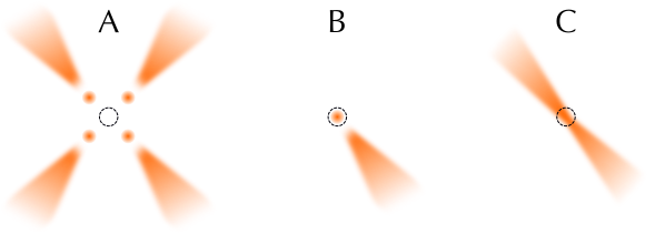
Figure 1: Diagram (not to scale) of the manual acquisition steps for the ESPRESSO observations described in this article. A: all 4LGSF lasers are propagating. The 4 laser guide-stars (orange dots) are positioned to a nominal square asterism using the LPC. From the instrument perspective, the up-link laser beams (visible up to $\sim$35 km of altitude) are located on the outside of the laser guide-stars (located at $\sim$90 km of altitude). B: using the LPC, a single laser guide-star is placed in centerfield. The propagation is stopped for all other laser guide-stars. C: the up-link beam is brought over the ESPRESSO fiber (black circle) using manual offsets applied to the jitter-loop mirror of the laser launch telescope. The focus of the telescope is adjusted to bring the beam better into focus at the location of the fiber.

III Results

We present in Fig. 2 and 3 a subset of the ESPRESSO spectrum of one up-link laser beam from the 4LGSF. Fig. 2 contains an overall view of the pure rotational Raman lines and the $\nu_{1\leftarrow 0}$ rotational-vibrational (ro-vibrational) Raman lines for ¹⁶O₂ and ¹⁴N₂, readily visible as a resolved forest of lines. In Fig. 3, we present a detailed view of the spectral regions located within $\pm$70 Å from the main laser line. To identify the specific origin of each line in the spectrum, we first compare it with the analytical predictions of the rotational and ro-vibrational Raman lines for homonuclear diatomic molecules treated as non-rigid singlet rotators (see the Supplemental Material for the full analytical derivation, which includes Refs. Herzberg, 1950; Shimauchi et al., 1995; Orlov et al., 1997; Bendtsen, 2001; Huber and Herzberg, 1979). We unambiguously detect pure rotational lines up to a molecular rotational quantum number $J=27$ for ¹⁶O₂ and $J=24$ for ¹⁴N₂. The lines in the $\nu_{1\leftarrow 0}$ ro-vibrational Q-branch of ¹⁴N₂ and ¹⁶O₂ are resolved from $J\gtrsim 4$, and unambiguously detected up to $J\sim 18$. For ¹⁶O₂, only lines associated with odd values of $J$ are detected, as expected from the selection rules imposed by quantum mechanics for homonuclear diatomic molecules with zero nuclear spin (Herzberg, 1950).

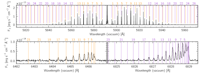
Figure 2: ESPRESSO view of the pure rotational Raman lines (top), and $Q$ branch of the ro-vibrational Raman lines of ¹⁶O₂ (bottom left) and ¹⁴N₂ (bottom right), associated with one 4LGSF up-link laser beam. Orange (for ¹⁶O₂) and purple (for ¹⁴N₂) lines mark the theoretical position of each Raman line derived with the model of non-rigid singlet diatomic rotators (see the Supplemental Material for details). Colored integers denote the rotational quantum number $J$ associated with the different analytical wavelength predictions. The CCD did saturate within $\pm$0.2 Å of the main laser line.

We also detect the pure rotational Raman lines from ¹⁴N¹⁵N (tentatively) up to $J=9$. These lines are detected with a signal-to-noise ratio $\cong 2\pm 1$: insufficient to formally rule out ¹⁴N₂⁺ as the molecule responsible, from the theoretical line wavelengths alone (see the Supplemental Material for details). To try to discriminate between ¹⁴N¹⁵N and ¹⁴N${}_{2}^{+}$, we assembled a simple model of two Gaussian lines with their dispersion tied, to individually fit each of the tentative ¹⁴N¹⁵N lines alongside the nearest ¹⁴N₂ line (i.e. associated to the same $J$-value). From a Markov-Chain Monte-Carlo sampling of the individual posterior distribution of each of the clearest 14 line pairs, assuming a least-square likelihood and flat priors with a lower bound of 0 for the line intensities and dispersion, we find no evidence for an alternating intensity pattern between lines associated with even and odd $J$ values, as one would expect from ¹⁴N⁺. On the other hand, we derive an overall line intensity ratio of 0.5${}^{+0.6}_{-0.3}$% (68% confidence level) with respect to the nearest ¹⁴N₂ lines, consistent with the atmospheric abundance ratio of ¹⁴N¹⁵N to ¹⁴N₂ (Junk and Svec, 1958). Clearly, deeper observations are necessary to confirm this identification.

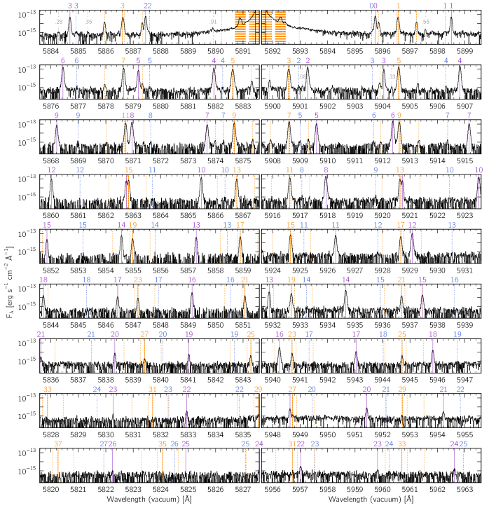
Figure 3: ESPRESSO spectrum of one 4LGSF up-link laser beam, focusing on the spectral regions containing pure rotational Raman lines. Each panel is 8 Å wide. For a given row, the left and right panels are equidistant from the main laser line at 5891.5912 Å (which is saturated). Pure rotational Raman lines, associated with the Stokes (right column) and anti-Stokes (left column) branches, are detected up to $J=27$ for ¹⁶O₂, $J=24$ for ¹⁴N₂, and $J=9$ for ¹⁴N¹⁵N. Solid orange, solid purple, and dash-dotted blue vertical lines mark the theoretical position of the pure rotational Raman lines of ¹⁶O₂, ¹⁴N₂, and ¹⁴N¹⁵N (respectively), when treated as non-rigid singlet diatomic rotators. The molecular rotational quantum number $J$ associated with each of these lines is indicated above them (only the ¹⁴N₂ $J=11$ anti-Stokes and $J=9,19$ Stokes lines are not tagged because of crowding). Dashed orange vertical lines, derived using a numerical model of ¹⁶O₂ accounting for the non-zero electronic spin of its ground state, highlight the fine-splitting of the pure rotational lines for this molecule. The nature of 6 lines (tagged with dotted grey vertical lines and the first two decimals of their wavelength in the top panels) remains unknown at this time.

Altogether, the analytical predictions account for most of the rotational and all of the ro-vibrational lines visible in the ESPRESSO spectrum, but fail to explain a series of fainter lines in the vicinity of the main laser line. We link the majority of these fainter lines to the existence of a non-zero electronic spin in the ground state ${}^{3}\Sigma_{g}^{-}$ of ¹⁶O₂. It is the interaction between this electronic spin and the molecular rotation that leads to the fine-splitting of the pure rotational Raman lines of ¹⁶O₂. From an exhaustive numerical modeling of this effect (see the Supplemental Material for details, which includes Refs. Yu et al., 2014, 2012; Drouin et al., 2012, 2013), we can successfully identify side-lines up to $N=9$ (where $N$ denotes the end-over-end rotation). We are left with 6 lines of (yet) unknown origin, all located within 13 Å from the main laser line (see Fig. 3).

IV Discussion

Up until now, the majority of observations of the up-link beams from laser guide-star systems at astronomical observatories would have resulted from the un-intentional collision between neighboring telescopes: an observational nuisance against which dedicated coordination tools were promptly developed (Summers et al., 2003, 2006; Amico et al., 2010, 2015). The fact remains, however, that propagating a laser beam through the atmosphere entails a range of physical phenomena, some of which are unrelated to the creation of artificial reference wavefront sources in support of AO systems. Raman scattering, in particular, implies that initially-monochromatic up-link laser beams possess a rich spectral signature, with numerous lines located several tens (for pure rotational Raman lines) up to several hundreds (for ro-vibrational Raman lines) of Å away from the main laser line. This may drive specific design choices for the next generation of optical AO instruments relying on laser guide-star systems. Under specific circumstances, for example with an on-axis laser guide-star system, pure rotational Raman lines more than one order of magnitude brighter than sky lines may potentially be found $\geq$50 Å away from the main laser line, as illustrated in Fig. 2. This might require the use of notch filters with a specific spectral width, should a cost-benefit analysis (balancing the scientific benefit(s) of increased wavelength coverage with the spectral contamination of rotational Raman lines) warrant it.

The inelastic Raman scattering of laser photons provides an ideal means to characterize the new ESPRESSO spectrograph at the VLT, and validate the wavelength solution of its data product over a spectral range of $\sim$1000 Å. The possible presence of wind along the line-of-sight (and thus the spectral shifting of the signal over time) implies that the Raman lines are not suitable to characterize the goal precision of 10 cm s^-1 over 10 years for radial velocity measurements with ESPRESSO. We find, however, that the accuracy with which the Raman lines ($<$5 fm for the case of ¹⁶O₂; see the Supplemental Material for details) and the exciting laser wavelength ($<$11.6 fm at the 3$\sigma$ level) are known is ideally matched to the target accuracy of ESPRESSO of 10 m s${}^{-1}\equiv$20 fm at the 4LGSF laser wavelength. The 4LGSF lasers have a spectral full-width at half maximum $\lesssim$5 MHz$\equiv$6 fm, so that the full-width at half maximum of the observed Raman lines is actually dominated by thermal broadening (of the order of 2.3 GHz for ¹⁴N₂ and 2.1 GHz for ¹⁶O₂ at 273 K). We find that measuring line-centroid values with an accuracy $<$10 fm requires peak-to-noise values larger than $\sim$200. This was achieved, for the pure-rotational Raman lines of ¹⁴N₂ and ¹⁶O₂ in the ESPRESSO spectrum presented in Fig. 3, up to $J\sim 15$ for both molecules.

The presence of wind shifts along the line of sight during such an observation can be easily minimized by pointing the telescope, on a quiet night, at a low airmass and at 90 deg from the dominant wind direction at high altitude. Doing so will restrict the spectral offsets caused by wind shifts to those associated with vertical motions, which can be expected to be less than 1 m s${}^{-1}\equiv$2 fm (Masciadri et al., 1999). We voluntarily do not present here the formal characterization of the spectral accuracy of ESPRESSO. It will be discussed by the instrument Consortium in a separate publication, together with the required modeling of the instrument line-spread-function which falls outside of the scope of this article.

The growing number of laser guide-star systems in operation (d’Orgeville and Fetzer, 2016) implies that the physics of Raman scattering is readily accessible to many professional astronomical telescopes world-wide: either directly, or via voluntary laser collisions with neighboring facilities (at sites hosting multiple observatories). As the power of new generations of laser guide-star systems increases, so does the flux of the associated Raman lines, which reduces the amount of time required to acquire spectra with sufficient signal-to-noise for an accurate instrumental characterization. The molecular physics potentially accessible via Raman scattering is undeniably very rich, as evidenced by its extensive use for atmospheric studies (Leonard, 1967; Cooney, 1968; Melfi et al., 1969; Melfi, 1972; Cooney, 1972; Keckhut et al., 1990; Whiteman et al., 1992; Heaps and Burris, 1996; Behrendt et al., 2002; Wandinger, 2005). For astronomers, the ¹⁴N₂ and ¹⁶O₂ molecules are undoubtedly the best molecules to focus on. As the prime constituents of Earth’s atmosphere, these homonuclear diatomic molecules will provide the strongest Raman signal, which is nowadays very well characterized. In essence, our ESPRESSO observation of one 4LGSF up-link laser beam paints the picture of a future in which laser guide-star systems at astronomical observatories will not only be thought of as mere sub-components of complex adaptive optics systems, but also as bright, flexible, and accurate calibration sources for characterizing new generations of astronomical spectrographs.

Appendix A Supplementary Material

Appendix B Rotational and ro-vibrational Raman line wavelengths for non-rigid singlet diatomic rotators

The vibro-rotational energy of a molecule, $E_{n}(J)$, for given vibrational quantum number $n$ and rotational quantum number $J$, can be expressed as:

$$E_{n}(J)=G_{n}+F_{n}(J),$$ (1)

with $G_{n}$ the vibrational component, and $F_{n}(J)$ the rotational component. Following Herzberg (1950), for diatomic molecules like ¹⁴N₂ with a ${}^{1}\Sigma$ electronic ground state or ¹⁶O₂ with a non-singlet electronic state but unresolved line splitting structure:

$$G_{n}\cong\omega_{e}(n+\frac{1}{2})-\omega_{e}X_{e}(n+\frac{1}{2})^{2}+\omega_{e}Y_{e}(n+\frac{1}{2})^{3}+\omega_{e}Z_{e}(n+\frac{1}{2})^{4},$$ (2)

and

$$F_{n}(J)\cong B_{n}J(J+1)-D_{n}J^{2}(J+1)^{2},$$ (3)

where

$$B_{n} \cong B_{e}-\alpha_{e}(n+\frac{1}{2})+\gamma_{e}(n+\frac{1}{2})^{2}$$ (4)

$$D_{n} \cong D_{e}+\beta_{e}(n+\frac{1}{2})$$ (5)

The adopted form of $F_{n}(J)$ assumes that molecules are non-rigid rotators, and includes the vibrational stretching of the molecular bond driven by rotation. The parameters $\omega_{e}$, $\omega_{e}X_{e}$, $\omega_{e}Y_{e}$, $\omega_{e}Z_{e}$, $B_{e}$, $\alpha_{e}$, $\gamma_{e}$, $D_{e}$ and $\beta_{e}$ are molecular constants typically expressed in cm^-1 (see Table 1). We adopt the values of Shimauchi et al. (1995) for ¹⁶O₂, Orlov et al. (1997) for ¹⁴N₂, Bendtsen (2001) for ¹⁴N¹⁵N, and Huber and Herzberg (1979) for ¹⁴N${}_{2}^{+}$.

Table 1: Molecular parameters adopted in our analytical model of non-rigid singlet diatomic rotators.

	$\omega_{e}$	$\omega_{e}X_{e}$	$\omega_{e}Y_{e}$	$\omega_{e}Z_{e}$	$B_{e}$	$\alpha_{e}$	$\gamma_{e}$	$D_{e}$	$\beta_{e}$
	[cm-1]	[cm-1]	[10-2 cm-1]	[10-3 cm-1]	[cm-1]	[10-2 cm-1]	[10-5 cm-1]	[10-6 cm-1]	[10-8 cm-1]
16O2	1580.161a	11.95127a	4.58489a	-1.87265a	1.44562a	1.59305a	0	4.839b	0
14N2	2358.54024c	14.30577c	-0.50668c	-0.1095c	1.9982399c	1.731281c	-2.8520c	5.7376c	1.02171c
14N15N	-	-	-	-	1.93184882d	1.646624d	-2.22d	5.3477d	1.06d
14N2+	-	-	-	-	1.93176b	1.881b	0	6.10b	0

The frequency shift of pure rotational Raman lines (with respect to the exciting frequency) associated with the elastic scattering of photons by non-rigid singlet diatomic molecules in their ground vibrational state ($n=0$), separated in the Stokes and anti-Stokes branches, can thus be expressed as:

$$\Delta\nu_{0}|_{\text{Stokes}}(J) = E_{0}(J+2)-E_{0}(J)$$

$$= (4B_{0}-6D_{0})(J+\frac{3}{2})-8D_{0}(J+\frac{3}{2})^{3}$$

for $J=0,1,\ldots$, and:

$$\Delta\nu_{0}|_{\text{anti-Stokes}}(J) = E_{0}(J-2)-E_{0}(J)$$

$$= (4B_{0}-6D_{0})(J-\frac{1}{2})-8D_{0}(J-\frac{1}{2})^{3}$$

for $J=1,2,\ldots$. The frequency shift (with respect to the exciting frequency) associated with the ro-vibrational Raman lines, separated in the $Q$, $S$ and $O$ branches, can be expressed as:

$$\Delta\nu_{1\leftarrow 0}|_{\text{Q}}(J) = E_{1}(J)-E_{0}(J)\text{ for }J=0,1,\ldots$$ (8)

$$\Delta\nu_{1\leftarrow 0}|_{\text{S}}(J) = E_{1}(J+2)-E_{0}(J)\text{ for }J=0,1,\ldots$$

$$\Delta\nu_{1\leftarrow 0}|_{\text{O}}(J) = E_{1}(J-2)-E_{0}(J)\text{ for }J=2,3,\ldots$$

For ¹⁶O₂, only odd values of $J$ are allowed. In our notation, the Raman shift of a given diatomic molecule, a notion often employed in the literature, corresponds to:

$$\Delta\nu_{1\leftarrow 0}|_{\text{Q}}(J=0) = G_{1}-G_{0}$$

$$= \omega_{e}-2\omega_{e}X_{e}+\frac{13}{4}\omega_{e}Y_{e}+5\omega_{e}Z_{e},$$

corresponding to 2329.913 cm^-1 for ¹⁴N₂ and 1556.398 cm^-1 for ¹⁶O₂, given the molecular constants of Table 1.

Appendix C Pure rotational Raman line wavelengths of ¹⁶O₂

The spectral resolution of ESPRESSO is such that the pure rotational fine-structure lines of ¹⁶O₂ are resolved in the 4LGSF up-link laser beam spectrum presented in the main article. To compute the theoretical wavelength of these lines, ¹⁶O₂ cannot be simply treated as a non-rigid singlet diatomic rotator, given the fact that this molecule has a ${}^{3}\Sigma$ electronic ground state. Due to the interaction of the electronic spin S$=1$ and end-over-end rotational angular momentum N, the rotational levels of ¹⁶O₂ are split into three fine-structure components, corresponding to the three ways of combining S and N vectorially to form the total angular momentum J. Each of these fine-structure levels is labelled with quantum numbers $N$ and $J$, with $J=N-1$, $N$, and $N+1$. Once again, the nuclear spin statistics of ¹⁶O₂ only allows odd values of $N$.

Yu et al. (2014) published the energies for all the fine-structure levels of ¹⁶O₂. To identify the associated lines in the spectrum acquired with ESPRESSO, we computed the pure rotational Raman shifts directly from these energy levels, with the following selection rules:

$$\Delta N=0,\pm 2\qquad\Delta J=0,\pm 1,\pm 2$$ (10)

The derived Raman shifts and predicted wavelengths for the pure rotational Raman lines of ¹⁶O₂ are presented in Table LABEL:table:params_SYu. Each rotational transition is labelled as ${}^{\Delta N}\Delta J(J,N)$, with the usual conventions that $Q\equiv(\Delta=0)$, $R\equiv(\Delta=+1)$, $P\equiv(\Delta=-1)$, $S\equiv(\Delta=+2)$ and $O\equiv(\Delta=-2)$. The strongest rotational transitions occur for $\Delta N=\Delta J$, while for $\Delta N=\Delta J\pm 1$ and $\Delta N=\Delta J\pm 2$, the transitions scale as $N^{-1}$ and $N^{-3}$, respectively. One should note that the derived rotational Raman shifts have an accuracy $<$0.0001 cm${}^{-1}\equiv 4$ fm at the 4LGSF laser wavelength, resulting from an extensive Hamiltonian model that was used to simultaneously fit the microwave, THz, infrared, visible and ultraviolet transitions of all six oxygen isotopologues (Yu et al., 2012; Drouin et al., 2012, 2013). In Table LABEL:table:params_SYu, wavelengths are purposely rounded to two digits (equivalent to a pm level) for simplicity. Readers interested in more precise values should derive them from the associated Raman shift $\Delta\nu$ via:

$$\lambda_{\text{Stokes}} = c\cdot\left(\frac{c}{\lambda_{\text{laser}}}-\Delta\nu\right)^{-1},\text{ and}$$ (11)

$$\lambda_{\text{anti-Stokes}} = c\cdot\left(\frac{c}{\lambda_{\text{laser}}}+\Delta\nu\right)^{-1},$$ (12)

with $c$ the speed of light.

In the ESPRESSO spectrum presented in the main article, the transitions in the immediate vicinity of the laser wavelength belong to the $\Delta N=0$, $\Delta J=\pm 2,$ transitions, i.e. the ^QO and ${}^{Q}S$ branches. The line at 5892.28 Å is a blend of all ${}^{Q}R$ and ${}^{Q}P$ transitions together with the ${}^{Q}S(0,1)$ line. The line at 5895.86 Å is ${}^{S}R(1,1)$. The line at 5896.55 Å is a blend of ${}^{S}S(1,1)$, ${}^{S}S(2,1)$ and the very weak ${}^{S}Q(2,1)$. The line at 5897.23 Å is a blend of ${}^{S}S(0,1)$ and ${}^{S}R(2,1)$. For $N\geq 3$, the line structure consists of a strong center line with a weak satellite line at each end. The strong center lines are from the blend of the three ${}^{S}S(J,N)$ lines and the very weak ${}^{S}Q(N+1,N)$ line. The weak satellites are from ${}^{S}R(N,N)$ and ${}^{S}R(N+1,N)$, respectively. Their intensities relative to the center line decrease very rapidly with $N$: in 900 s on-source with ESPRESSO, we detected the weak satellite lines up to $N=9$.

Table 2: Theoretical ¹⁶O₂ pure rotational Raman shifts and associated Stokes and anti-Stokes line wavelengths, computed from the energies of the molecule’s fine-structure levels derived by Yu et al. (2014), for the main exciting wavelength of the 4LGSF lasers.

(
${}^{\Delta N}\Delta J$ (	$J$ ,	$N$ )	$\Delta\nu$	anti-Stokes	Stokes
			[cm-1]	[Å]	[Å]
${}^{Q}S$ (	4 ,	5 )	0.0239	5891.58	5891.60
${}^{Q}O$ (	8 ,	7 )	0.0424	5891.58	5891.61
${}^{Q}O$ (	10 ,	9 )	0.0943	5891.56	5891.62
${}^{Q}S$ (	2 ,	3 )	0.1347	5891.54	5891.64
${}^{Q}O$ (	12 ,	11 )	0.1397	5891.54	5891.64
${}^{Q}O$ (	14 ,	13 )	0.1816	5891.53	5891.65
${}^{Q}O$ (	16 ,	15 )	0.2213	5891.51	5891.67
${}^{Q}O$ (	18 ,	17 )	0.2597	5891.50	5891.68
${}^{Q}O$ (	20 ,	19 )	0.2971	5891.49	5891.69
${}^{Q}O$ (	22 ,	21 )	0.3338	5891.48	5891.71
${}^{Q}O$ (	24 ,	23 )	0.3701	5891.46	5891.72
${}^{Q}O$ (	26 ,	25 )	0.4059	5891.45	5891.73
${}^{Q}O$ (	28 ,	27 )	0.4415	5891.44	5891.74
${}^{Q}O$ (	30 ,	29 )	0.4768	5891.43	5891.76
${}^{Q}O$ (	32 ,	31 )	0.5120	5891.41	5891.77
${}^{Q}O$ (	34 ,	33 )	0.5470	5891.40	5891.78
${}^{Q}O$ (	36 ,	35 )	0.5818	5891.39	5891.79
${}^{Q}O$ (	38 ,	37 )	0.6166	5891.38	5891.81
${}^{Q}O$ (	40 ,	39 )	0.6513	5891.36	5891.82
${}^{Q}O$ (	42 ,	41 )	0.6860	5891.35	5891.83
${}^{Q}O$ (	44 ,	43 )	0.7206	5891.34	5891.84
${}^{Q}O$ (	46 ,	45 )	0.7551	5891.33	5891.85
${}^{Q}O$ (	48 ,	47 )	0.7896	5891.32	5891.86
${}^{Q}O$ (	50 ,	49 )	0.8241	5891.31	5891.88
${}^{Q}O$ (	52 ,	51 )	0.8586	5891.29	5891.89
${}^{Q}O$ (	54 ,	53 )	0.8930	5891.28	5891.90
${}^{Q}O$ (	56 ,	55 )	0.9274	5891.27	5891.91
${}^{Q}O$ (	58 ,	57 )	0.9619	5891.26	5891.93
${}^{Q}O$ (	60 ,	59 )	0.9963	5891.24	5891.94
${}^{Q}O$ (	62 ,	61 )	1.0307	5891.23	5891.95
${}^{Q}O$ (	64 ,	63 )	1.0652	5891.22	5891.96
${}^{Q}R$ (	64 ,	65 )	1.4478	5891.09	5892.09
${}^{Q}R$ (	62 ,	63 )	1.4645	5891.08	5892.10
${}^{Q}R$ (	60 ,	61 )	1.4812	5891.08	5892.10
${}^{Q}R$ (	58 ,	59 )	1.4980	5891.07	5892.11
${}^{Q}R$ (	56 ,	57 )	1.5147	5891.06	5892.12
${}^{Q}R$ (	54 ,	55 )	1.5315	5891.06	5892.12
${}^{Q}R$ (	52 ,	53 )	1.5482	5891.05	5892.13
${}^{Q}R$ (	50 ,	51 )	1.5651	5891.05	5892.13
${}^{Q}R$ (	48 ,	49 )	1.5819	5891.04	5892.14
${}^{Q}R$ (	46 ,	47 )	1.5988	5891.04	5892.15
${}^{Q}R$ (	44 ,	45 )	1.6156	5891.03	5892.15
${}^{Q}R$ (	42 ,	43 )	1.6326	5891.02	5892.16
${}^{Q}R$ (	40 ,	41 )	1.6496	5891.02	5892.16
${}^{Q}R$ (	38 ,	39 )	1.6666	5891.01	5892.17
${}^{Q}R$ (	36 ,	37 )	1.6836	5891.01	5892.18
${}^{Q}R$ (	34 ,	35 )	1.7008	5891.00	5892.18
${}^{Q}R$ (	32 ,	33 )	1.7180	5890.99	5892.19
${}^{Q}R$ (	30 ,	31 )	1.7352	5890.99	5892.19
${}^{Q}R$ (	28 ,	29 )	1.7526	5890.98	5892.20
${}^{Q}R$ (	26 ,	27 )	1.7701	5890.98	5892.21
${}^{Q}R$ (	24 ,	25 )	1.7878	5890.97	5892.21
${}^{Q}R$ (	22 ,	23 )	1.8056	5890.96	5892.22
${}^{Q}R$ (	20 ,	21 )	1.8236	5890.96	5892.22
${}^{Q}R$ (	18 ,	19 )	1.8420	5890.95	5892.23
${}^{Q}R$ (	16 ,	17 )	1.8607	5890.94	5892.24
${}^{Q}P$ (	2 ,	1 )	1.8768	5890.94	5892.24
${}^{Q}R$ (	14 ,	15 )	1.8801	5890.94	5892.24
${}^{Q}R$ (	12 ,	13 )	1.9003	5890.93	5892.25
${}^{Q}R$ (	10 ,	11 )	1.9217	5890.92	5892.26
${}^{Q}R$ (	8 ,	9 )	1.9455	5890.92	5892.27
${}^{Q}P$ (	4 ,	3 )	1.9496	5890.91	5892.27
${}^{Q}R$ (	6 ,	7 )	1.9735	5890.91	5892.28
${}^{Q}P$ (	6 ,	5 )	1.9877	5890.90	5892.28
${}^{Q}R$ (	4 ,	5 )	2.0116	5890.89	5892.29
${}^{Q}P$ (	8 ,	7 )	2.0159	5890.89	5892.29
${}^{Q}P$ (	10 ,	9 )	2.0398	5890.88	5892.30
${}^{Q}P$ (	12 ,	11 )	2.0614	5890.88	5892.31
${}^{Q}P$ (	14 ,	13 )	2.0818	5890.87	5892.31
${}^{Q}S$ (	0 ,	1 )	2.0843	5890.87	5892.31
${}^{Q}R$ (	2 ,	3 )	2.0843	5890.87	5892.31
${}^{Q}P$ (	16 ,	15 )	2.1014	5890.86	5892.32
${}^{Q}P$ (	18 ,	17 )	2.1204	5890.85	5892.33
${}^{Q}P$ (	20 ,	19 )	2.1391	5890.85	5892.33
${}^{Q}P$ (	22 ,	21 )	2.1575	5890.84	5892.34
${}^{Q}P$ (	24 ,	23 )	2.1756	5890.84	5892.35
${}^{Q}P$ (	26 ,	25 )	2.1937	5890.83	5892.35
${}^{Q}P$ (	28 ,	27 )	2.2116	5890.82	5892.36
${}^{Q}P$ (	30 ,	29 )	2.2294	5890.82	5892.36
${}^{Q}P$ (	32 ,	31 )	2.2472	5890.81	5892.37
${}^{Q}P$ (	34 ,	33 )	2.2649	5890.81	5892.38
${}^{Q}P$ (	36 ,	35 )	2.2826	5890.80	5892.38
${}^{Q}P$ (	38 ,	37 )	2.3003	5890.79	5892.39
${}^{Q}P$ (	40 ,	39 )	2.3179	5890.79	5892.40
${}^{Q}P$ (	42 ,	41 )	2.3355	5890.78	5892.40
${}^{Q}P$ (	44 ,	43 )	2.3531	5890.77	5892.41
${}^{Q}P$ (	46 ,	45 )	2.3708	5890.77	5892.41
${}^{Q}P$ (	48 ,	47 )	2.3884	5890.76	5892.42
${}^{Q}P$ (	50 ,	49 )	2.4060	5890.76	5892.43
${}^{Q}P$ (	52 ,	51 )	2.4236	5890.75	5892.43
${}^{Q}P$ (	54 ,	53 )	2.4413	5890.74	5892.44
${}^{Q}P$ (	56 ,	55 )	2.4589	5890.74	5892.44
${}^{Q}P$ (	58 ,	57 )	2.4766	5890.73	5892.45
${}^{Q}P$ (	60 ,	59 )	2.4943	5890.73	5892.46
${}^{Q}P$ (	62 ,	61 )	2.5120	5890.72	5892.46
${}^{Q}P$ (	64 ,	63 )	2.5297	5890.71	5892.47
${}^{Q}R$ (	0 ,	1 )	3.9611	5890.22	5892.97
${}^{S}R$ (	1 ,	1 )	12.2918	5887.33	5895.86
${}^{S}Q$ (	2 ,	1 )	14.1686	5886.68	5896.51
${}^{S}S$ (	2 ,	1 )	14.3033	5886.63	5896.56
${}^{S}S$ (	1 ,	1 )	14.3761	5886.60	5896.59
${}^{S}S$ (	0 ,	1 )	16.2529	5885.95	5897.24
${}^{S}R$ (	2 ,	1 )	16.2529	5885.95	5897.24
${}^{S}R$ (	3 ,	3 )	23.8629	5883.32	5899.89
${}^{S}Q$ (	4 ,	3 )	25.8125	5882.65	5900.56
${}^{S}S$ (	4 ,	3 )	25.8364	5882.64	5900.57
${}^{S}S$ (	3 ,	3 )	25.8745	5882.62	5900.59
${}^{S}S$ (	2 ,	3 )	25.9473	5882.60	5900.61
${}^{S}R$ (	4 ,	3 )	27.8241	5881.95	5901.27
${}^{S}R$ (	5 ,	5 )	35.3953	5879.33	5903.90
${}^{S}S$ (	6 ,	5 )	37.3406	5878.66	5904.58
${}^{S}S$ (	5 ,	5 )	37.3688	5878.65	5904.59
${}^{S}Q$ (	6 ,	5 )	37.3830	5878.64	5904.60
${}^{S}S$ (	4 ,	5 )	37.4069	5878.64	5904.60
${}^{S}R$ (	6 ,	5 )	39.3565	5877.96	5905.28
${}^{S}R$ (	7 ,	7 )	46.9115	5875.35	5907.92
${}^{S}S$ (	8 ,	7 )	48.8331	5874.69	5908.59
${}^{S}S$ (	7 ,	7 )	48.8570	5874.68	5908.60
${}^{S}S$ (	6 ,	7 )	48.8850	5874.67	5908.61
${}^{S}Q$ (	8 ,	7 )	48.9274	5874.66	5908.62
${}^{S}R$ (	8 ,	7 )	50.8729	5873.98	5909.30
${}^{S}R$ (	9 ,	9 )	58.4156	5871.38	5911.94
${}^{S}S$ (	10 ,	9 )	60.3156	5870.73	5912.60
${}^{S}S$ (	9 ,	9 )	60.3373	5870.72	5912.61
${}^{S}S$ (	8 ,	9 )	60.3610	5870.71	5912.62
${}^{S}Q$ (	10 ,	9 )	60.4553	5870.68	5912.65
${}^{S}R$ (	10 ,	9 )	62.3771	5870.02	5913.32
${}^{S}R$ (	11 ,	11 )	69.9076	5867.43	5915.96
${}^{S}S$ (	12 ,	11 )	71.7875	5866.78	5916.61
${}^{S}S$ (	11 ,	11 )	71.8079	5866.77	5916.62
${}^{S}S$ (	10 ,	11 )	71.8294	5866.76	5916.63
${}^{S}Q$ (	12 ,	11 )	71.9690	5866.72	5916.68
${}^{S}R$ (	12 ,	11 )	73.8693	5866.06	5917.34
${}^{S}R$ (	13 ,	13 )	81.3867	5863.48	5919.98
${}^{S}S$ (	14 ,	13 )	83.2472	5862.84	5920.63
${}^{S}S$ (	13 ,	13 )	83.2668	5862.83	5920.64
${}^{S}S$ (	12 ,	13 )	83.2870	5862.82	5920.64
${}^{S}Q$ (	14 ,	13 )	83.4685	5862.76	5920.71
${}^{S}R$ (	14 ,	13 )	85.3486	5862.11	5921.37
${}^{S}R$ (	15 ,	15 )	92.8515	5859.54	5924.00
${}^{S}S$ (	16 ,	15 )	94.6932	5858.90	5924.64
${}^{S}S$ (	15 ,	15 )	94.7123	5858.90	5924.65
${}^{S}S$ (	14 ,	15 )	94.7316	5858.89	5924.66
${}^{S}Q$ (	16 ,	15 )	94.9529	5858.81	5924.73
${}^{S}R$ (	16 ,	15 )	96.8137	5858.18	5925.39
${}^{S}R$ (	17 ,	17 )	104.3004	5855.61	5928.02
${}^{S}S$ (	18 ,	17 )	106.1237	5854.98	5928.66
${}^{S}S$ (	17 ,	17 )	106.1424	5854.98	5928.67
${}^{S}S$ (	16 ,	17 )	106.1612	5854.97	5928.67
${}^{S}Q$ (	18 ,	17 )	106.4208	5854.88	5928.76
${}^{S}R$ (	18 ,	17 )	108.2628	5854.25	5929.41
${}^{S}R$ (	19 ,	19 )	115.7317	5851.69	5932.04
${}^{S}S$ (	20 ,	19 )	117.5370	5851.07	5932.67
${}^{S}S$ (	19 ,	19 )	117.5553	5851.07	5932.68
${}^{S}S$ (	18 ,	19 )	117.5737	5851.06	5932.69
${}^{S}Q$ (	20 ,	19 )	117.8708	5850.96	5932.79
${}^{S}R$ (	20 ,	19 )	119.6944	5850.34	5933.43
${}^{S}R$ (	21 ,	21 )	127.1436	5847.79	5936.06
${}^{S}S$ (	22 ,	21 )	128.9310	5847.18	5936.69
${}^{S}S$ (	21 ,	21 )	128.9492	5847.17	5936.69
${}^{S}S$ (	20 ,	21 )	128.9673	5847.16	5936.70
${}^{S}Q$ (	22 ,	21 )	129.3011	5847.05	5936.82
${}^{S}R$ (	22 ,	21 )	131.1067	5846.43	5937.45
${}^{S}R$ (	23 ,	23 )	138.5344	5843.89	5940.07
${}^{S}S$ (	24 ,	23 )	140.3042	5843.29	5940.70
${}^{S}S$ (	23 ,	23 )	140.3222	5843.28	5940.70
${}^{S}S$ (	22 ,	23 )	140.3400	5843.28	5940.71
${}^{S}Q$ (	24 ,	23 )	140.7101	5843.15	5940.84
${}^{S}R$ (	24 ,	23 )	142.4978	5842.54	5941.47
${}^{S}R$ (	25 ,	25 )	149.9023	5840.01	5944.09
${}^{S}S$ (	26 ,	25 )	151.6545	5839.42	5944.71
${}^{S}S$ (	25 ,	25 )	151.6724	5839.41	5944.71
${}^{S}S$ (	24 ,	25 )	151.6900	5839.40	5944.72
${}^{S}Q$ (	26 ,	25 )	152.0959	5839.27	5944.86
${}^{S}R$ (	26 ,	25 )	153.8661	5838.66	5945.49
${}^{S}R$ (	27 ,	27 )	161.2453	5836.15	5948.10
${}^{S}S$ (	28 ,	27 )	162.9801	5835.56	5948.71
${}^{S}S$ (	27 ,	27 )	162.9980	5835.55	5948.72
${}^{S}S$ (	26 ,	27 )	163.0155	5835.55	5948.72
${}^{S}Q$ (	28 ,	27 )	163.4569	5835.40	5948.88
${}^{S}R$ (	28 ,	27 )	165.2096	5834.80	5949.50
${}^{S}R$ (	29 ,	29 )	172.5618	5832.30	5952.10
${}^{S}S$ (	30 ,	29 )	174.2793	5831.71	5952.71
${}^{S}S$ (	29 ,	29 )	174.2971	5831.71	5952.72
${}^{S}S$ (	28 ,	29 )	174.3144	5831.70	5952.73
${}^{S}Q$ (	30 ,	29 )	174.7913	5831.54	5952.89
${}^{S}R$ (	30 ,	29 )	176.5265	5830.95	5953.51
${}^{S}R$ (	31 ,	31 )	183.8498	5828.46	5956.11
${}^{S}S$ (	32 ,	31 )	185.5501	5827.88	5956.71
${}^{S}S$ (	31 ,	31 )	185.5678	5827.88	5956.72
${}^{S}S$ (	30 ,	31 )	185.5851	5827.87	5956.72
${}^{S}Q$ (	32 ,	31 )	186.0971	5827.70	5956.90
${}^{S}R$ (	32 ,	31 )	187.8150	5827.11	5957.51
${}^{S}R$ (	33 ,	33 )	195.1076	5824.64	5960.10
${}^{S}S$ (	34 ,	33 )	196.7907	5824.07	5960.70
${}^{S}S$ (	33 ,	33 )	196.8084	5824.06	5960.71
${}^{S}S$ (	32 ,	33 )	196.8256	5824.05	5960.71
${}^{S}Q$ (	34 ,	33 )	197.3725	5823.87	5960.91
${}^{S}R$ (	34 ,	33 )	199.0733	5823.29	5961.51
${}^{S}R$ (	35 ,	35 )	206.3332	5820.83	5964.09
${}^{S}S$ (	36 ,	35 )	207.9992	5820.27	5964.69
${}^{S}S$ (	35 ,	35 )	208.0168	5820.26	5964.69
${}^{S}S$ (	34 ,	35 )	208.0340	5820.26	5964.70
${}^{S}Q$ (	36 ,	35 )	208.6158	5820.06	5964.90
${}^{S}R$ (	36 ,	35 )	210.2995	5819.49	5965.50
${}^{S}R$ (	37 ,	37 )	217.5248	5817.04	5968.08
${}^{S}S$ (	38 ,	37 )	219.1738	5816.48	5968.66
${}^{S}S$ (	37 ,	37 )	219.1914	5816.48	5968.67
${}^{S}S$ (	36 ,	37 )	219.2085	5816.47	5968.68
${}^{S}Q$ (	38 ,	37 )	219.8251	5816.26	5968.90
${}^{S}R$ (	38 ,	37 )	221.4917	5815.70	5969.49
${}^{S}R$ (	39 ,	39 )	228.6807	5813.27	5972.05
${}^{S}S$ (	40 ,	39 )	230.3126	5812.72	5972.63
${}^{S}S$ (	39 ,	39 )	230.3302	5812.71	5972.64
${}^{S}S$ (	38 ,	39 )	230.3472	5812.71	5972.65
${}^{S}Q$ (	40 ,	39 )	230.9986	5812.49	5972.88
${}^{S}R$ (	40 ,	39 )	232.6481	5811.93	5973.47

Table 2: continued.

References

- Bonaccini Calia et al. (2014a) D. Bonaccini Calia, W. Hackenberg, R. Holzlöhner, S. Lewis, and T. Pfrommer, “The Four-Laser Guide Star Facility: Design considerations and system implementation,” Advanced Optical Technologies 3, 345–361 (2014a).
- Arsenault et al. (2013) R. Arsenault, P.-Y. Madec, J. Paufique, P. La Penna, S. Stroebele, E. Vernet, J.-F. Pirard, W. Hackenberg, H. Kuntschner, J. Kolb, et al., “The ESO Adaptive Optics Facility under Test,” in Proceedings of the Third AO4ELT Conference (2013) p. 118.
- Moussaoui et al. (2010) N. Moussaoui, B. R. Clemesha, R. Holzlöhner, D. M. Simonich, D. Bonaccini Calia, W. Hackenberg, and P. P. Batista, “Statistics of the sodium layer parameters at low geographic latitude and its impact on adaptive-optics sodium laser guide star characteristics,” Astron. Astrophys. 511, A31 (2010).
- Neichel et al. (2013) B. Neichel, C. D’Orgeville, J. Callingham, F. Rigaut, C. Winge, and G. Trancho, “Characterization of the sodium layer at Cerro Pachón, and impact on laser guide star performance,” Mon. Not. R. Astron. Soc. 429, 3522–3532 (2013).
- Pfrommer and Hickson (2014) T. Pfrommer and P. Hickson, “High resolution mesospheric sodium properties for adaptive optics applications,” Astron. Astrophys. 565, A102 (2014).
- Holzlöhner et al. (2010) R. Holzlöhner, S. M. Rochester, D. Bonaccini Calia, D. Budker, J. M. Higbie, and W. Hackenberg, “Optimization of cw sodium laser guide star efficiency,” Astron. Astrophys. 510, A20 (2010).
- Friedenauer et al. (2012) A. Friedenauer, V. Karpov, D. Wei, M. Hager, B. Ernstberger, W. R. L. Clements, and W. G. Kaenders, “RFA-based 589-nm guide star lasers for ESO VLT: A paradigm shift in performance, operational simplicity, reliability, and maintenance,” in Adaptive Optics Systems III, Procspie, Vol. 8447 (2012) p. 84470F.
- Enderlein et al. (2014) M. Enderlein, A. Friedenauer, R. Schwerdt, P. Rehme, D. Wei, V. Karpov, B. Ernstberger, P. Leisching, W. R. L. Clements, and W. G. Kaenders, “Series production of next-generation guide-star lasers at TOPTICA and MPBC,” in Adaptive Optics Systems IV, Procspie, Vol. 9148 (2014) p. 914807.
- Lewis et al. (2014) S. Lewis, D. B. Calia, B. Buzzoni, P. Duhoux, G. Fischer, I. Guidolin, A. Haimerl, W. Hackenberg, R. Hinterschuster, R. Holzlöhner, et al., “Laser Guide Star Facility Upgrade,” The Messenger 155, 6–11 (2014).
- Stuik et al. (2006) R. Stuik, R. Bacon, R. Conzelmann, B. Delabre, E. Fedrigo, N. Hubin, M. Le Louarn, and S. Ströbele, “GALACSI - The ground layer adaptive optics system for MUSE,” New Astronomy Reviews 49, 618–624 (2006).
- La Penna et al. (2016) P. La Penna, E. Aller Carpentier, J. Argomedo, R. Arsenault, R. D. Conzelmann, B. Delabre, R. Donaldson, F. Gago, P. Gutierrez-Cheetam, N. Hubin, et al., “AOF: Standalone test results of GALACSI,” in Society of Photo-Optical Instrumentation Engineers (SPIE) Conference Series, Procspie, Vol. 9909 (2016) p. 99092Z.
- Paufique et al. (2010) J. Paufique, A. Bruton, A. Glindemann, A. Jost, J. Kolb, L. Jochum, M. Le Louarn, M. Kiekebusch, N. Hubin, P.-Y. Madec, et al., “GRAAL: A seeing enhancer for the NIR wide-field imager Hawk-I,” in Adaptive Optics Systems II, Procspie, Vol. 7736 (2010) p. 77361P.
- Bacon et al. (2010) R. Bacon, M. Accardo, L. Adjali, H. Anwand, S. Bauer, I. Biswas, J. Blaizot, D. Boudon, S. Brau-Nogue, J. Brinchmann, et al., “The MUSE second-generation VLT instrument,” in Ground-Based and Airborne Instrumentation for Astronomy III, Procspie, Vol. 7735 (2010) p. 773508.
- Kissler-Patig et al. (2008) M. Kissler-Patig, J.-F. Pirard, M. Casali, A. Moorwood, N. Ageorges, C. Alves de Oliveira, P. Baksai, L. R. Bedin, E. Bendek, P. Biereichel, et al., “HAWK-I: The high-acuity wide-field K-band imager for the ESO Very Large Telescope,” Astron. Astrophys. 491, 941–950 (2008).
- Siebenmorgen et al. (2011) R. Siebenmorgen, G. Carraro, E. Valenti, M. Petr-Gotzens, G. Brammer, E. Garcia, and M. Casali, “The Science Impact of HAWK-I,” The Messenger 144, 9–12 (2011).
- Vogt et al. (2017) F. P. A. Vogt, D. Bonaccini Calia, W. Hackenberg, C. Opitom, M. Comin, L. Schmidtobreik, J. Smoker, I. Blanchard, M. Espinoza Contreras, I. Aranda, et al., “Detection and Implications of Laser-Induced Raman Scattering at Astronomical Observatories,” Physical Review X 7, 021044 (2017).
- Bonaccini Calia et al. (2014b) D. Bonaccini Calia, M. Centrone, F. Pedichini, A. Ricciardi, A. Cerruto, and F. Ambrosino, “Laser guide star pointing camera for ESO LGS Facilities,” in Adaptive Optics Systems IV, Procspie, Vol. 9148 (2014) p. 91483P.
- Vogt et al. (2018) F. P. A. Vogt, J. Luis Álvarez, D. Bonaccini Calia, W. Hackenberg, P. Bourget, I. Aranda, C. Bellhouse, I. Blanchard, S. Cerda, C. Cid, et al., “Raman-scattered laser guide-star photons to monitor the scatter of astronomical telescope mirrors,” Astron. Astrophys. 618, L7 (2018).
- Pepe et al. (2010) F. A. Pepe, S. Cristiani, R. Rebolo Lopez, N. C. Santos, A. Amorim, G. Avila, W. Benz, P. Bonifacio, A. Cabral, P. Carvas, et al., “ESPRESSO: The Echelle spectrograph for rocky exoplanets and stable spectroscopic observations,” in Ground-Based and Airborne Instrumentation for Astronomy III, Procspie, Vol. 7735 (2010) p. 77350F.
- Pepe et al. (2013) F. Pepe, S. Cristiani, R. Rebolo, N. C. Santos, H. Dekker, D. Mégevand, F. M. Zerbi, A. Cabral, P. Molaro, P. Di Marcantonio, et al., “ESPRESSO — An Echelle SPectrograph for Rocky Exoplanets Search and Stable Spectroscopic Observations,” The Messenger 153, 6–16 (2013).
- Lo Curto et al. (2012) G. Lo Curto, L. Pasquini, A. Manescau, R. Holzwarth, T. Steinmetz, T. Wilken, R. Probst, T. Udem, T. W. Hänsch, J. González Hernández, et al., “Astronomical Spectrograph Calibration at the Exo-Earth Detection Limit,” The Messenger 149, 2–6 (2012).
- Monet et al. (2003) D. G. Monet, S. E. Levine, B. Canzian, H. D. Ables, A. R. Bird, C. C. Dahn, H. H. Guetter, H. C. Harris, A. A. Henden, S. K. Leggett, et al., “The USNO-B Catalog,” A.J. 125, 984–993 (2003).
- Duhoux et al. (2014) P. Duhoux, J. Knudstrup, P. Lilley, P. Di Marcantonio, R. Cirami, and M. Mannetta, “VLT instruments: Industrial solutions for non-scientific detector systems,” in Software and Cyberinfrastructure for Astronomy III, Procspie, Vol. 9152 (2014) p. 91520I.
- Kerber et al. (2012) F. Kerber, T. Rose, A. Chacón, O. Cuevas, H. Czekala, R. Hanuschik, Y. Momany, J. Navarrete, R. R. Querel, A. Smette, et al., “A water vapour monitor at Paranal Observatory,” in Ground-Based and Airborne Instrumentation for Astronomy IV, Procspie, Vol. 8446 (2012) p. 84463N.
- Kerber et al. (2014) F. Kerber, R. R. Querel, R. Rondanelli, R. Hanuschik, M. van den Ancker, O. Cuevas, A. Smette, J. Smoker, T. Rose, and H. Czekala, “An episode of extremely low precipitable water vapour over Paranal observatory,” Mon. Not. R. Astron. Soc. 439, 247–255 (2014).
- Herzberg (1950) G. Herzberg, Molecular Spectra and Molecular Structure. Vol.1: Spectra of Diatomic Molecules, 2nd ed. (Van Nostrand Reinhold, New York, 1950).
- Shimauchi et al. (1995) M. Shimauchi, T. Miura, and H. Takuma, “Determination of Molecular Constnts of the X3g- State of O2,” Japanese Journal of Applied Physics 34, L1689 (1995).
- Orlov et al. (1997) M. L. Orlov, J. F. Ogilvie, and J. W. Nibler, “High-Resolution Coherent Raman Spectra of Vibrationally Excited14N2and15N2,” Journal of Molecular Spectroscopy 185, 128–141 (1997).
- Bendtsen (2001) J. Bendtsen, “High-resolution Fourier transform Raman spectra of the fundamental bands of 14N15N and 15N2,” Journal of Raman Spectroscopy 32, 989–995 (2001).
- Huber and Herzberg (1979) K.-P. Huber and G. Herzberg, Molecular Spectra and Molecular Structure. Vol.4: Constants of Diatomic Molecules (Van Nostrand Reinhold, New York, 1979).
- Junk and Svec (1958) G. Junk and H. J. Svec, “The absolute abundance of the nitrogen isotopes in the atmosphere and compressed gas from various sources,” Geochimica et Cosmochimica Acta 14, 234–243 (1958).
- Yu et al. (2014) S. Yu, B. J. Drouin, and C. E. Miller, “High resolution spectral analysis of oxygen. IV. Energy levels, partition sums, band constants, RKR potentials, Franck-Condon factors involving the X3g-, a1g and b1g+ states,” The Journal of Chemical Physics 141, 174302 (2014).
- Yu et al. (2012) S. Yu, C. E. Miller, B. J. Drouin, and H. S. P. Müller, “High resolution spectral analysis of oxygen. I. Isotopically invariant Dunham fit for the X3g-, a1g, b1g+ states,” The Journal of Chemical Physics 137, 024304 (2012).
- Drouin et al. (2012) B. J. Drouin, H. Gupta, S. Yu, C. E. Miller, and H. S. P. Müller, “High resolution spectral analysis of oxygen. II. Rotational spectra of a1g O2 isotopologues,” The Journal of Chemical Physics 137, 024305 (2012).
- Drouin et al. (2013) B. J. Drouin, S. Yu, B. M. Elliott, T. J. Crawford, and C. E. Miller, “High resolution spectral analysis of oxygen. III. Laboratory investigation of the airglow bands,” The Journal of Chemical Physics 139, 144301 (2013).
- Summers et al. (2003) D. Summers, B. Gregory, P. J. Stomski, Jr., A. Brighton, R. J. Wainscoat, P. L. Wizinowich, W. Gaessler, J. Sebag, C. Boyer, T. Vermeulen, et al., “Implementation of a laser traffic control system supporting laser guide star adaptive optics on Mauna Kea,” in Adaptive Optical System Technologies II, Procspie, Vol. 4839 (2003) pp. 440–451.
- Summers et al. (2006) D. Summers, N. Apostolakos, R. Rutten, and G. Talbot, “Second generation laser traffic control: Algorithm changes supporting Mauna Kea, La Palma, and future multi-telescope laser sites,” in Society of Photo-Optical Instrumentation Engineers (SPIE) Conference Series, Procspie, Vol. 6272 (2006) p. 627244.
- Amico et al. (2010) P. Amico, R. D. Campbell, and J. C. Christou, “Laser operations at the 8-10m class telescopes Gemini, Keck, and the VLT: Lessons learned, old and new challenges,” in Observatory Operations: Strategies, Processes, and Systems III, Procspie, Vol. 7737 (2010) p. 77370A.
- Amico et al. (2015) P. Amico, P. Santos, D. Summers, P. Duhoux, R. Arsenault, T. Bierwirth, H. Kuntschner, P.-Y. Madec, M. Prümm, and M. Rejkuba, “The First Component of the Adaptive Optics Facility Enters Operations: The Laser Traffic Control System on Paranal,” The Messenger 162, 19–23 (2015).
- Masciadri et al. (1999) E. Masciadri, J. Vernin, and P. Bougeault, “3D mapping of optical turbulence using an atmospheric numerical model. I. A useful tool for the ground-based astronomy,” Astron. Astrophys.Supplement Series 137, 185–202 (1999).
- d’Orgeville and Fetzer (2016) C. d’Orgeville and G. J. Fetzer, “Four generations of sodium guide star lasers for adaptive optics in astronomy and space situational awareness,” in Adaptive Optics Systems V, Procspie, Vol. 9909 (2016) pp. 99090R–99090R–18.
- Leonard (1967) D. A. Leonard, “Observation of Raman Scattering from the Atmosphere using a Pulsed Nitrogen Ultraviolet Laser,” Nature 216, 142–143 (1967).
- Cooney (1968) J. Cooney, “Measurements on the Raman component of laser atmospheric backscatter,” Applied Physics Letters 12, 40–42 (1968).
- Melfi et al. (1969) S. H. Melfi, J. Lawrence, and M. McCormick, “Observation of Raman scattering by water vapor in the atmosphere,” Applied Physics Letters 15, 295–297 (1969).
- Melfi (1972) S. H. Melfi, “Remote measurements of the atmosphere using Raman scattering,” Applied Optics 11, 1605 (1972).
- Cooney (1972) J. Cooney, “Measurement of Atmospheric Temperature Profiles by Raman Backscatter,” Journal of Applied Meteorology 11, 108–112 (1972).
- Keckhut et al. (1990) P. Keckhut, M. L. Chanin, and A. Hauchecorne, “Stratosphere temperature measurement using Raman lidar,” Applied Optics 29, 5182–5186 (1990).
- Whiteman et al. (1992) D. N. Whiteman, S. H. Melfi, and R. A. Ferrare, “Raman lidar system for the measurement of water vapor and aerosols in the Earth’s atmosphere,” Applied Optics 31, 3068 (1992).
- Heaps and Burris (1996) W. S. Heaps and J. Burris, “Airborne Raman lidar,” Applied Optics 35, 7128–7135 (1996).
- Behrendt et al. (2002) A. Behrendt, T. Nakamura, M. Onishi, R. Baumgart, and T. Tsuda, “Combined Raman lidar for the measurement of atmospheric temperature, water vapor, particle extinction coefficient, and particle backscatter coefficient,” Applied Optics 41, 7657 (2002).
- Wandinger (2005) U. Wandinger, “Raman Lidar,” in Lidar: Range-Resolved Optical Remote Sensing of the Atmosphere, Springer Series in Optical Sciences, edited by C. Weitkamp (Springer New York, New York, NY, 2005) pp. 241–271.
- Hunter (2007) J. D. Hunter, “Matplotlib: A 2D Graphics Environment,” Computing in Science and Engineering 9, 90–95 (2007).
- Astropy Collaboration et al. (2013) Astropy Collaboration, T. P. Robitaille, E. J. Tollerud, P. Greenfield, M. Droettboom, E. Bray, T. Aldcroft, M. Davis, A. Ginsburg, A. M. Price-Whelan, et al., “Astropy: A community Python package for astronomy,” Astron. Astrophys. 558, A33 (2013).
- Astropy Collaboration et al. (2018) Astropy Collaboration, A. M. Price-Whelan, B. M. Sipőcz, H. M. Günther, P. L. Lim, S. M. Crawford, S. Conseil, D. L. Shupe, M. W. Craig, N. Dencheva, et al., “The Astropy Project: Building an Open-science Project and Status of the v2.0 Core Package,” A.J. 156, 123 (2018).
- Robitaille and Bressert (2012) T. Robitaille and E. Bressert, “APLpy: Astronomical Plotting Library in Python,” Astrophysics Source Code Library , ascl:1208.017 (2012).
- Vogt (2018a) F. P. A. Vogt, “Fcmaker: Creating ESO-compliant finding charts for Observing Blocks on p2,” Astrophysics Source Code Library , ascl:1806.027 (2018a).
- Vogt (2018b) F. P. A. Vogt, “Fcmaker: Automating the creation of ESO-compliant finding charts for Observing Blocks on p2,” Astronomy and Computing 25, 81–88 (2018b).
- Ginsburg et al. (2017) A. Ginsburg, M. Parikh, J. Woillez, A. Groener, S. Liedtke, B. Sipocz, T. Robitaille, C. Deil, B. Svoboda, E. Tollerud, et al., “Astroquery: Access to online data resources,” Astrophysics Source Code Library , ascl:1708.004 (2017).
- Morris et al. (2018) B. M. Morris, E. Tollerud, B. Sipőcz, C. Deil, S. T. Douglas, J. Berlanga Medina, K. Vyhmeister, T. R. Smith, S. Littlefair, A. M. Price-Whelan, et al., “Astroplan: An Open Source Observation Planning Package in Python,” A.J. 155, 128 (2018).
- Foreman-Mackey et al. (2013) D. Foreman-Mackey, D. W. Hogg, D. Lang, and J. Goodman, “Emcee: The MCMC Hammer,” Publ. Astron. Soc. Pac. 125, 306 (2013).
- Bonnarel et al. (2000) F. Bonnarel, P. Fernique, O. Bienaymé, D. Egret, F. Genova, M. Louys, F. Ochsenbein, M. Wenger, and J. G. Bartlett, “The ALADIN interactive sky atlas. A reference tool for identification of astronomical sources,” Astron. Astrophys.Supplement Series 143, 33–40 (2000).
- Joye and Mandel (2003) W. A. Joye and E. Mandel, “New Features of SAOImage DS9,” in Astronomical Data Analysis Software and Systems XII ASP Conference Series, Vol. 295 (2003) p. 489.