Flavor changing neutral current decays $t\to cX$ ($X=\gamma,\,g,\,Z,\,H$) and $t\to c\bar{\ell}\ell$ ($\ell=\mu,\,\tau$) via scalar leptoquarks

Abstract

The flavor changing neutral current decays $t\to cX$ ($X=\gamma,\,g,\,Z,\,H$) and $t\to c\bar{\ell}\ell$ ($\ell=\mu,\,\tau$) are studied in a renormalizable scalar leptoquark (LQ) model with no proton decay, where a scalar $SU(2)$ doublet with hypercharge $Y=7/6$ is added to the standard model, yielding a non-chiral LQ $\Omega_{5/3}$. Analytical results for the one-loop (tree-level) contributions of a scalar LQ to the $f_{i}\to f_{j}X$ ($f_{i}\to f_{j}\bar{f}_{m}f_{l}$) decays, with $f_{a}=q_{a},\ell_{a}$, are presented. We consider the scenario where $\Omega_{5/3}$ couples to the fermions of the second and third families, with its right- and left-handed couplings obeying $\lambda_{R}^{\ell u_{i}}/\lambda_{L}^{\ell u_{i}}=O(\epsilon)$, where $\epsilon$ parametrizes the relative size between these couplings. The allowed parameter space is then found via the current constraints on the muon $(g-2)$, the $\tau\to\mu\gamma$ decay, the LHC Higgs boson data, and the direct LQ searches at the LHC. For $m_{\Omega_{5/3}}=1$ TeV and $\epsilon=10^{-3}$, we find that the $t\to cX$ branching ratios are of similar size and can be as large as $10^{-8}$ in a tiny area of the parameter space, whereas ${\rm Br}(t\to c\bar{\tau}\tau)$ [${\rm Br}(t\to c\bar{\mu}\mu)$] can be up to $10^{-6}$ ($10^{-7}$).

1 Introduction

The conjecture that lepton number is the fourth color quantum number was put forward long ago in the context of an $SU(4)_{R}\times SU(4)_{L}\times SU(4^{\prime})$ theory Pati:1973uk ; Pati:1974yy , which requires the presence of new gauge and scalar bosons carrying both lepton and baryon number. Such particles, dubbed leptoquarks (LQs) since transform leptons into quarks and vice versa, appear naturally in grand unified theories Georgi:1974sy ; Fritzsch:1974nn ; Ramond:1976jg ; Senjanovic:1982ex ; Frampton:1989fu , but they are also predicted in other well motivated theories, such as technicolor Ellis:1980hz ; Farhi:1980xs ; Hill:2002ap , models with composite fermions Schrempp:1984nj ; Buchmuller:1985nn ; Gripaios:2009dq , superstring-inspired ${\rm E}_{6}$ models Witten:1985xc ; Hewett:1988xc , models with extended scalar sectors Davies:1990sc ; Arnold:2013cva , etc. However, LQs with lepton and baryon number violating interactions can give rise to dangerous effects such as large lepton flavor violating interactions (LFV) or tree-level-induced proton decay. The latter implies that, unless an extra symmetry is invoked to forbid diquark couplings, LQ masses must be as heavy as the Planck scale, thereby rendering unobservable effects on low energy processes. Therefore, only those theories with renormalizable lepton and baryon number conserving LQ interactions are phenomenologically appealing. LQ phenomenology and low-energy constraints on the parameter space of the most representative LQ models have been widely discussed (see Davidson:1993qk for instance). For a more up-to-date review on LQ physics we refer the reader to Ref. Dorsner:2016wpm . It turns out that vector LQ masses and couplings are tightly constrained by experimental data, therefore the study of scalar LQs has been favored in the literature. In this work we are interested in a simple renormalizable LQ model with no proton decay where the presence of relatively light scalar LQs can still be compatible with low energy constraints from experimental data Dorsner:2009cu ; Arnold:2013cva ; Cheung:2015yga . In such a model, scalar LQs are introduced in the standard model (SM) via a doublet of $SU(2)$.

In the SM flavor changing neutral currents (FCNCs) can arise up to the one-loop level or higher orders of perturbation theory, but are additionally suppressed by the so-called Glashow–Iliopoulos–Maiani (GIM) mechanism. On the other hand, the SM forbids LFV effects at any order, though experimental evidences hint that neutrinos are massive, thereby implying that LFV effects should be present in nature indeed. No evidences of large FCNCs transitions have yet been experimentally observed, so the search for this class of effects is a must in the physics program of any particle collider. While FCNC transition between fermions of the second and first family are considerably constrained by experimental data, transitions involving the fermions of the third and second generation have no such strong restrictions. In this regard, FCNC top quark transitions stand out among the most widely studied processes at the CERN LHC. This stems from the fact that in spite of having negligible rates in the SM, they can have a considerable enhancement in beyond the SM theories and could be at the reach of detection.

The scalar particle discovered at the LHC in 2012 seems to be consistent with the SM Higgs boson, but several of its properties remain to be tested more accurately, such as its couplings to light fermions. The LHC also offers great potential to search for some exotic Higgs decay channels that are highly suppressed or forbidden in the SM. Along these lines, there has been considerably interest in the study of the LFV Higgs boson decay $H\to\bar{\ell}_{i}\ell_{j}$, which was first studied in DiazCruz:1999xe ; Han:2000jz and has been the focus of great attention recently. Although an apparent excess of the $H\to\tau\mu$ branching ratio, with a significance of $2.4\,\sigma$, was observed at the LHC Run 1 Khachatryan:2015kon , it was not confirmed in Run-2 data. The LFV Higgs boson decay $H\to\bar{\ell}_{i}\ell_{j}$ has been widely studied in several extension models. In particular, in the LQ model of Ref. Cheung:2015yga , the $H\to\tau\mu$ rate is predicted to be at the reach of experimental detection in some regions of the allowed parameter space. On the other hand, in the quark sector, apart from the FCNC Higgs boson decay into light quarks $H\to qq^{\prime}$, the FCNC top quark decay $t\to cH$ has also been widely studied along with other decays such as $t\to c\gamma$, $t\to cZ$ and $t\to cg$.

At hadron colliders, the dominant top quark production mechanisms are gluon fusion and quark annihilation. The former is the main top quark production process at the LHC (about 90 % at $\sqrt{s}=$14 TeV), with a small percentage due to quark annihilation. The millions of yearly top quark events at the LHC would allow experimentalist to search for its FCNCs decays such as $t\to cX$ ($V=\gamma,\,Z,\,H$), whose rates are negligibly small in the SM Eilam:1990zc ; DiazCruz:1989ub ; Mele:1998ag :

$${\rm Br}^{\rm SM}(t\to cg) =10^{-8},$$ (1)

$${\rm Br}^{\rm SM}(t\to c\gamma) =10^{-10},$$ (2)

$${\rm Br}^{\rm SM}(t\to cZ) =10^{-13},$$ (3)

$${\rm Br}^{\rm SM}(t\to cH) =10^{-13}.$$ (4)

These rates however can be several orders of magnitude larger in several SM extensions, such as two-Higgs doublet models Eilam:1990zc ; Diaz:2001vj , supersymmetric models Couture:1994rr ; Li:1993mg ; Lopez:1997xv ; Yang:1997dk , left-right supersymmetric models Frank:2005vd , extra dimensions GonzalezSprinberg:2007zz , models with an extra neutral gauge boson CorderoCid:2005kp , 331 models Cortes-Maldonado:2013rca , etc. Therefore, any experimental evidence of these FCNCs top quark and Higgs boson decay channels may shed light on the underlying fundamental theory of particle interactions.

In this work we focus on the study of the FCNC decays $t\to cX$ ($X=\gamma,\,g,\,Z,\,H$) in a simple renormalizable scalar LQ model in which there is no proton decay induced via tree-level LQ exchange, where these processes arise at one-loop level at the lowest order of perturbation theory. As a by-product, we present the exact results for the one-loop LQ scalar contribution to the $H\to\bar{f}_{j}f_{i}$ decay width, which follows easily from the $f_{i}\to f_{j}H$ decay width by crossing symmetry. For completeness, we also consider in our study the tree-level FCNC decay $t\to c\bar{\ell}\ell$ ($\ell=\mu,\,\tau$), which in fact can have larger branching ratios than those of the one-loop induced decays.

The rest of this presentation is as follows. In Sec. 2 we briefly discuss the framework of the LQ model we are interested in. Sec. 3 is devoted to present the general calculation of the FCNC decay amplitudes and decay widths. For the one-loop induced decays we express the amplitudes in terms of both Passarino-Veltman scalar functions and Feynman parameter integrals. We present a discussion on the constraints on the LQ couplings from experimental data in Sec. 5, followed by the numerical analysis of the FCNCs Higgs boson transitions in Sec. 6. The conclusions and outlook are presented in Sec. 7. Finally, a few lengthy formulas for the loop integrals are presented in the Appendices.

2 A simple scalar LQ model

Rather than considering a specific theory, a convenient strategy to study the LQ phenomenology is via a model-independent approach through an effective lagrangian. One can thus focus on the low energy LQ interactions and, without loss of generality, disregard the complex framework of the ultraviolet completion, which is not relevant for the phenomenology below the TeV scale. The most general dimension-four $SU(3)_{c}\times SU(2)_{L}\times U(1)_{Y}$-invariant effective interactions of scalar and vector LQs, respecting both lepton and baryon number was first presented in Buchmuller:1986zs and has been analyzed recently in Dorsner:2016wpm . In this work we consider a simple renormalizable LQ model in which it is not necessary to invoke an extra symmetry to forbid the proton decay. A single $SU(2)$ doublet with hypercharge $7/6$ is added to the SM, giving rise to two LQs with electric charges $5/3e$ and $2/3e$. The former one is a non-chiral LQ that couples to up quarks and charged leptons, thereby giving rise to FCNC top quark and Higgs boson decays at the one-loop level, but also to the $t\to c\bar{\ell}\ell$ decay at the tree-level. The phenomenology of this model was studied in Arnold:2013cva and bounds on its couplings to a lepton-quark pairs from the experimental constraints on the muon anomalous magnetic dipole moment and the LFV tau decay $\tau\to\mu\gamma$ were obtained in Bolanos:2013tda . We first start by discussing the corresponding LQ couplings to quarks and leptons and afterwards we discuss the remaining interactions.

In the model we are interested in, a scalar LQ representation $R_{2}$ with $SU(3)\times SU(2)\times U(1)$ quantum numbers $(3,2,7/6)$ is introduced. This LQ doublet has the following renormalizable zero-fermion-number interactions Buchmuller:1986zs

$${\cal L}_{F=0}=h^{ij}_{2L}R_{2}^{T}\bar{u}^{i}_{R}i\tau_{2}L^{j}_{L}+h^{ij}_{2R}\bar{Q}^{i}_{L}e^{j}_{R}R_{2}+{\rm H.c.},$$ (5)

where ${L_{L}^{i}}$ and ${Q_{L}^{i}}$ are $SU(2)_{L}$ left-handed lepton and quark doublets, whereas $e^{i}_{R}$ and $q^{i}_{R}$ are singlets, with $i$ and $j$ being generation indices.

After rotating to the LQ mass eigenstates $\Omega_{5/3}$ and $\Omega_{2/3}$, where the subscript denotes the electric charge in units of $e$, we obtain the following interaction Lagrangian

$${\cal L}_{F=0}=\bar{e}^{i}\left(\lambda_{L}^{ij}P_{L}+\lambda_{R}^{ij}P_{R}\right)u^{j}\Omega_{5/3}^{*}+\bar{e}^{i}\eta_{R}^{ij}P_{R}d^{j}\Omega_{2/3}^{*}+{\rm H.c.},$$ (6)

where $P_{L,R}$ are the chiral projection operators. We are interested in the effects of the non-chiral LQ $\Omega_{5/3}$ on the FCNC decays of the top quark and the Higgs boson. Since there are stringent constraints on the LQ couplings to the fermions of the two first families, in our study below we will consider that $\Omega_{5/3}$ only couples to the second and third generation fermions.

Apart from the LQ interaction to up quarks and charged lepton pairs, which follow easily from the above expression, for our calculation we also need the LQ couplings to both the photon and the $Z$ gauge boson, which are extracted from the LQ kinetic terms:

$${\cal L}_{S}=\frac{1}{2}(D_{\mu}R_{2})^{\dagger}D_{\mu}R_{2},$$ (7)

where the $SU(2)_{L}\times U(1)_{Y}$ covariant derivative is given by

$$D_{\mu}R_{2}=\left(\partial_{\mu}+ig\frac{\tau^{i}}{2}W^{i}+ig^{\prime}\frac{7}{6}B^{\mu}\right)R_{2}.$$ (8)

Therefore, in the mass eigenstate basis we have

$${\cal L}_{S} \supset i\frac{5e}{3}\Omega_{5/3}\overleftrightarrow{\partial_{\mu}}\Omega_{5/3}^{*}A^{\mu}-\frac{ig}{c_{W}}g_{Z\Omega_{5/3}\Omega_{5/3}}{\Omega_{5/3}}\overleftrightarrow{\partial_{\mu}}\Omega_{5/3}^{*}Z^{\mu}$$ (9)

$$+ {\rm H.c.},$$

where $g_{Z\Omega_{5/3}\Omega_{5/3}}=1/2-5/3s_{W}^{2}$.

Finally, we consider the following renormalizable effective LQ interactions to the SM Higgs doublet $\Phi$

$$\mathcal{L}=\left(M_{R_{2}}^{2}+\lambda_{R_{2}}\Phi^{\dagger}\Phi\right)\left(R_{2}^{\dagger}R_{2}\right),$$ (10)

where $M_{R_{2}}$ is the LQ mass. From here we obtain the Higgs boson coupling to $\Omega_{5/3}$:

$${\mathcal{L}}\supset\lambda_{\Omega_{5/3}}vH\Omega_{5/3}^{*}\Omega_{5/3}.$$ (11)

For easy reference, we also present the SM Feynman rules for the interaction of the photon and the $Z$ gauge boson with a fermion-antifermion pair:

$$\bar{f}fA_{\mu} :-ieQ_{f}\gamma_{\mu},$$ (12)

$$\bar{f}fZ_{\mu} :-i\frac{g}{2c_{W}}\gamma_{\mu}(g^{f}_{L}P_{L}+g^{f}_{R}P_{R})$$ (13)

where $g_{L}^{f}=2T^{3}_{f}-2Q_{f}s_{W}^{2}$ and $g_{R}^{f}=-2Q_{f}s_{W}^{2}$, with $T^{3}_{f}=1/2(-1/2)$ for up (down) fermions and $Q_{f}$ the fermion charge in units of that of the positron.

The corresponding Feynman rules follow straightforwardly from the above Lagrangians and are shown in Fig. 1. Below we present the calculation of the FCNC $t\to cX$ and $t\to c\bar{\ell}\ell$ decays.

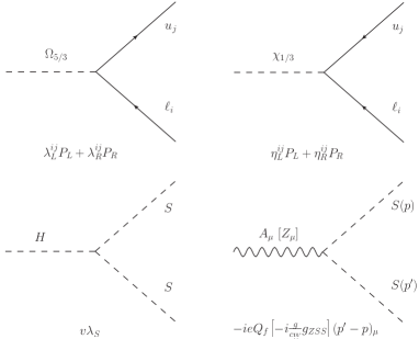
Figure 1: Feynman rules necessary for the calculation of the contribution of the scalar LQ $\Omega_{5/3}$ to the $t\to cX$ ($X=\gamma,\,Z,\,H$) decays. For completeness we also include the Feynman rules for the LQ singlet $\chi_{1/3}$ of the model discussed in Cheung:2015yga as our results are also valid for its contribution, thus $S$ stands for $\Omega_{5/3}$ and $\chi_{1/3}$, with $g_{ZSS}=\frac{1}{2}-\frac{10}{3}s_{W}^{2}\;(-\frac{2}{3}s_{W}^{2})$ for $S=\Omega_{5/3}$ ($\chi_{1/3}$).

3 LQ contribution to the FCNC $t\to cX$ decays

We now discuss the calculation of the FCNC $t\to cX$ decays, which in our scalar LQ model proceed at the one-loop level at the lowest order of perturbation theory. For the sake of completeness we present the most general expressions for the $f_{i}\to f_{j}X$ decays with $X=\gamma,\,Z,\,H$ and $f_{i,j}$ quarks or leptons. From our result for the $q_{i}\to q_{j}\gamma$ decay, that for the $q_{i}\to q_{j}g$ decay will follow easily as discussed below.

For the calculation of the loop integrals, we use both the Feynman parameter technique and the Passarino-Veltman reduction scheme, which allows one to cross-check the results. For the algebra we used the Mathematica software routines along with the FeynCalc package Shtabovenko:2016sxi . It is worth mentioning that our results are also valid for the contribution of the LQ singlet $\chi_{1/3}$ of the model of Ref. Cheung:2015yga , where the LQ contribution to the $H\to\mu\tau$ was discussed. The Feynman rules for such a LQ are of Majorana-like type (there are two fermion-flow arrows clashing into a vertex as shown in Fig. 1) and they require a special treatment. We have followed the approach of Ref. Moore:1984eg and found that the results for the contribution of LQ $\Omega_{5/3}$ to the $f_{i}\to f_{j}X$ decays are also valid for the contributions of LQ $\chi_{1/3}$ after replacing the respective coupling constants. A similar result was found for the contribution of single and doubly charged scalars to the muon anomalous MDM Moore:1984eg .

3.1 $f_{i}\to f_{j}V$ ($V=\gamma,\,Z$) decays

This decay proceeds at the lowest order via the Feynman diagrams of Fig. 2, where the internal fermion is a lepton (quark) provided that the external fermions are quarks (leptons).

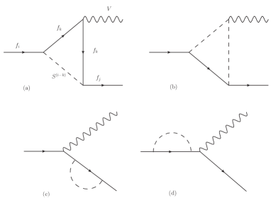
Figure 2: LQ contribution to the decay $f_{i}\to f_{j}V$ ($V=\gamma,Z$) , where $f_{i}$ and $f_{j}$ are charged leptons (quarks) and $f_{k}$ is a quark (lepton). Here $Q_{i-k}$ is the LQ charge in units of $e$. Analogue diagrams give rise to the $f_{i}\to f_{j}H$ decay with the $V$ gauge boson replaced by the Higgs boson. As far as the $q_{i}\to q_{j}g$ decay is concerned, there is only contribution from diagrams b) to d) as the internal fermion is a lepton.

The ultraviolet divergences cancel out when summing over all the partial amplitudes. The most general invariant amplitude can be written as

$${\cal M}(f_{i}\to f_{j}V) = \bar{f}_{j}\Big{(}\frac{iL^{V}}{m_{i}}\,\sigma_{\mu\nu}P_{L}q^{\nu}+\frac{iR^{V}}{m_{i}}\,\sigma_{\mu\nu}P_{R}q^{\nu}$$ (14)

$$+ L^{{}^{\prime}V}\,\gamma^{\mu}P_{L}+R^{{}^{\prime}V}\,\gamma^{\mu}P_{R}\Big{)}f_{i}\epsilon(q)^{\mu},$$

where the monopole terms $L^{{}^{\prime}\gamma}$ and $R^{{}^{\prime}\gamma}$ vanish for the $f_{i}\to f_{j}\gamma$ decay due to gauge invariance: the bubble diagrams only give contributions to the monopole terms, which are canceled out by those arising from the triangle diagrams. The corresponding $L^{V}$, $R^{V}$, $L^{{}^{\prime}Z}$, and $R^{{}^{\prime}Z}$ form factors are presented in terms of Passarino-Veltman scalar functions in A.

After averaging (summing) over polarizations of the initial (final) fermion and gauge boson, we use the respective two-body decay width formula, which reduces to

$$\Gamma(f_{i}\to f_{j}V) =\frac{\lambda^{1/2}(m_{i}^{2},m_{V}^{2},m_{j}^{2})}{32\pi m_{i}^{3}}\Bigg{(}f_{ij}\left(|L^{V}|^{2}+|R^{V}|^{2}\right)$$

$$+g_{ij}\left(|L^{{}^{\prime}V}|^{2}+|R^{{}^{\prime}V}|^{2}\right)$$

$$+3\left(m_{j}^{2}-m_{i}^{2}+m_{V}^{2}\right)\left(L^{{}^{\prime}V}R^{V*}+L^{V}R^{{}^{\prime}V*}\right)$$

$$+\frac{3m_{j}}{m_{i}}\left(m_{i}^{2}-m_{j}^{2}+m_{V}^{2}\right)\left(L^{V}L^{{}^{\prime}V*}+R^{V}R^{{}^{\prime}V*}\right)$$

$$-\frac{3m_{j}m_{V}^{2}}{m_{i}}{\rm Re}\left(L^{V}R^{V*}\right)$$

$$-12m_{i}m_{j}{\rm Re}\left(L^{{}^{\prime}V}R^{{}^{\prime}V*}\right)\Bigg{)},$$ (15)

with $f_{ij}=\frac{1}{m_{i}^{2}}\left(2\left(m_{i}^{2}-m_{j}^{2}\right)^{2}-\left(m_{i}^{2}+m_{j}^{2}\right)m_{V}^{2}-m_{V}^{4}\right)$ and $g_{ij}=\frac{1}{m_{V}^{2}}\left(\left(m_{i}^{2}-m_{j}^{2}\right)^{2}+\left(m_{i}^{2}+m_{j}^{2})\right)m_{V}^{2}-2m_{V}^{4}\right)$. The so-called triangle function is given by

$$\lambda(x,y,z)=x^{2}+y^{2}+z^{2}-2(xy+xz+yz).$$ (16)

For the $f_{i}\to f_{j}\gamma$ decay, Eq. (3.1) reduces to

$$\Gamma(f_{i}\to f_{j}\gamma) =\frac{m_{i}}{16\pi}\left(1-\left(\frac{m_{j}}{m_{i}}\right)^{2}\right)^{3}\left(|L^{\gamma}|^{2}+|R^{\gamma}|^{2}\right).$$ (17)

3.2 $q_{i}\to q_{j}g$ decay

This one-loop FCNC process is induced by Feynman diagrams similar to those shown in Fig. 2, except that there is no contribution from Feynman diagram of type a) as the internal fermion is a lepton. The Feynman rules necessary for the calculation are presented in Fig. 3.

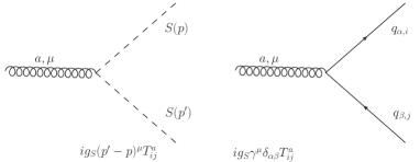
Figure 3: Feynman rules that are required for the calculation of the contribution of a scalar LQ to the $t\to cg$ decay. Here $T^{a}$ are the $SU(3)_{c}$ generators in the fundamental representation.

The $q_{i}\to q_{j}g$ amplitude can be written as

$${\cal M}(q_{i}\to q_{j}g) =\bar{q}_{j}T^{a}\Big{(}\frac{iL^{g}}{m_{i}}\,\sigma_{\mu\nu}P_{L}q^{\nu}+\frac{iR^{g}}{m_{i}}\,\sigma_{\mu\nu}P_{R}q^{\nu}\Big{)}q_{i}$$

$$\times\epsilon(q)_{\mu},$$ (18)

where the $L^{g}$ and $R^{g}$ coefficients can be obtained from Eqs. (A.1.1) and (A.2.1) of A once the replacements $Q_{k}\to 0$, $Q_{S}\to 1$, and $N_{c}e\to g_{s}$ are done. After averaging (summing) over initial (final) polarizations and colors, we obtain the average square amplitude and thereby the corresponding decay width, which has the same form of Eq. (17), though we must multiply the right-hand side by the color factor $C_{F}=4/3$.

3.3 $f_{i}\to f_{j}H$ decay

We now present the invariant amplitude for the LQ contribution to the $f_{i}\to f_{j}H$ decay, which is induced at the one-loop level by Feynman diagrams analogue to those shown in Fig. 2, but with the gauge boson $V$ replaced by the Higgs boson $H$. We have found that while the amplitude of Feynman diagram (d) is ultraviolet finite, that of Feyman diagram (a) has ultraviolet divergences, but they are canceled out by those arising from the bubble diagrams (b) and (c). After some algebra, the invariant amplitude can be cast in the form

$${\cal M}(f_{i}\to f_{j}H)=\bar{f}_{j}\left(F_{L}P_{L}+F_{R}P_{R}\right)f_{i},$$ (19)

where the $F_{L}$ and $F_{R}$ form factors are presented in B in terms of Passarino-Veltman scalar functions and Feynman parameter integrals.

After summing (averaging) over the polarizations of the final (initial) fermion, we plug the average squared amplitude into the two-body decay width formula to obtain

$$\Gamma(f_{i}\to f_{j}H) =\frac{\lambda^{1/2}(m_{i}^{2},m_{H}^{2},m_{j}^{2})}{8m_{i}^{3}\pi}\Big{(}\left(|F_{L}|^{2}+|F_{R}|^{2}\right)p_{i}\cdot p_{j}$$

$$+2m_{i}m_{j}{\rm Re}\left(F_{L}F_{R}^{*}\right)\Big{)},$$ (20)

with $p_{i}\cdot p_{j}=(m_{i}^{2}+m_{j}^{2}-m_{H}^{2})/2$.

3.4 $H\to\bar{f}_{j}f_{i}$ decay

As a by-product we present the $H\to\bar{f}_{j}f_{i}$ decay width, which follows straightforwardly from the above results by crossing symmetry. Although the scalar LQ contribution to the LFV decay $H\to\tau\mu$ has been already presented in the zero lepton mass approximation Cheung:2015yga ; Kim:2018oih ; Cai:2017wry ; Bauer:2015knc , we now present the exact one-loop calculation for the $H\to\bar{f}_{j}f_{i}$ decay width. It reads

$$\Gamma(H\to f_{i}f_{j}) =\frac{\lambda^{1/2}(m_{H}^{2},m_{i}^{2},m_{j}^{2})}{16\pi m_{H}^{3}}\Big{(}\left(|F_{L}|^{2}+|F_{R}|^{2}\right)p_{i}\cdot p_{j}$$

$$-2m_{i}m_{j}{\rm Re}(F_{L}F_{R}^{*})\Big{)},$$ (21)

where $\Gamma(H\to f_{i}f_{j})=\Gamma(H\to\bar{f}_{i}f_{j})+\Gamma(H\to\bar{f}_{j}f_{i})$. Also $p_{j}\cdot p_{j}=(m_{H}^{2}-(m_{i}^{2}+m_{j}^{2}))/2$, and the $F_{L}$ and $F_{R}$ form factors are the same as those presented in B for the $f_{i}\to f_{j}H$ decay as discussed in C.

4 Three-body tree-level decay $f_{i}\to f_{j}{\bar{f}}_{m}f_{l}$

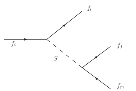
Figure 4: Feynman diagram for the tree-level FCNC decay $f_{i}\to f_{j}{\bar{f}}_{m}f_{l}$ induced by a scalar LQ. Here $f_{l}$ and $f_{m}$ are leptons (quarks) if $f_{i}$ and $f_{j}$ are quarks (leptons).

Finally we discuss the calculation of the three-body decay $t\to c\bar{\ell}\ell$. Following our calculation approach, we consider the general decay $f_{i}\to f_{j}{\bar{f}}_{m}f_{l}$, where $f_{l}$ and $f_{m}$ are leptons (quarks) if $f_{i}$ and $f_{j}$ are quarks (leptons). This process is induced by a scalar LQ at the tree-level via the Feynman diagram of Fig. 4. We denote the four-momentum of fermion $f_{a}$ ($a=i,j,l,m$) by $p_{a}$. The corresponding decay width can be written as

$$\Gamma(f_{i}\to f_{j}\bar{f}_{m}f_{l})=\frac{m_{i}}{256\pi^{3}}\int_{x_{ji}}^{x_{jf}}\int_{x_{li}}^{x_{lf}}|\mathcal{\overline{M}}|^{2}dx_{j}dx_{l}.$$ (22)

In the center-of-mass frame of the decaying fermion, the scaled variables $x_{a}$ ($a=j,l,m$) are given as $x_{a}=2E_{a}/m_{a}$. From energy conservation, these variables obey $x_{j}+x_{l}+x_{m}=2$. The kinematic limits in Eq. (22) are in turn

$$x_{jf} = 2\sqrt{\mu_{j}},$$ (23)

$$x_{ji} = 1+\mu_{j}-\mu_{l}-\mu_{m}-2\sqrt{\mu_{l}\mu_{m}},$$ (24)

$$x_{li,lf} = \frac{1}{2(1-x_{j}+\mu_{j})}\Bigl{[}(2-x_{j})(1+\mu_{j}+\mu_{l}-\mu_{m}-x_{j})$$ (25)

$$\mp \sqrt{x_{j}^{2}-4\mu_{j}}\lambda^{1/2}(1+\mu_{j}-x_{i},\mu_{l},\mu_{m})\Bigr{]},$$

where $\mu_{a}=m_{a}^{2}/m_{i}^{2}$ $(a=j,l,m)$.

The square average amplitude can be expressed as

$$|\mathcal{\overline{M}}|^{2} = \frac{2(p_{j}\cdot p_{m}(|\lambda^{jm}_{L}|^{2}+|\lambda^{jm}_{R}|^{2})-2m_{m}m_{j}\lambda^{jm}_{L}\lambda^{jm}_{R})}{(m_{m}^{2}+m_{j}^{2}-m_{S}^{2}-2p_{j}\cdot p_{m})^{2}}$$ (26)

$$\times \Bigl{(}(m_{l}^{2}+p_{l}\cdot p_{m}+p_{j}\cdot p_{l})(|\lambda^{il}_{L}|^{2}+|\lambda^{il}_{R}|^{2})$$

$$+ 2m_{i}m_{l}\lambda^{il}_{L}\lambda^{il}_{R}\Bigr{)},$$

where the scalar products can be written as

$$p_{l}\cdot p_{m} = \frac{m_{i}^{2}}{2}(1+\mu_{j}-\mu_{l}-\mu_{m}-x_{j}),$$ (27)

$$p_{j}\cdot p_{m} = \frac{m_{i}^{2}}{2}(1-\mu_{j}+\mu_{l}-\mu_{m}-x_{l}),$$ (28)

$$p_{j}\cdot p_{l} = \frac{m_{i}^{2}}{2}(1-\mu_{j}+\mu_{m}-\mu_{l}-x_{m}).$$ (29)

The integration of Eq. (22) can be performed numerically.

5 Constraints on the parameter space of the scalar LQ models

We now consider the LQ model introduced above and present an analysis of the constraints on the LQ couplings to SM fermions and the Higgs boson. While the LQ couplings to fermions can be obtained from the muon anomalous MDM and LFV tau decays, the LQ coupling to a Higgs boson pair can be extracted from the constraint on the $H\gamma\gamma$ and $Hgg$ couplings obtained by the ATLAS and CMS collaborations Khachatryan:2016vau .

5.1 Constraints on scalar LQ masses

The phenomenology of the scalar LQ doublet $R_{2}$ has been long studied in the literature Shanker:1982nd ; Davidson:1993qk ; Mizukoshi:1994zy ; Arnold:2013cva ; Dorsner:2013tla ; Bolanos:2013tda , and constraints on their mass and couplings have been derived from the $Z\to b\bar{b}$ decay, the muon anomalous MDM, and LFV decays. Since low energy physics strongly constrains the LQ couplings to the first-generation fermions, it is usually assumed that the only non-negligible couplings are those to the fermions of the second and third generations. The most stringent current constraint on the mass of the scalar LQ doublet $R_{2}$ masses is $m_{\Omega_{2/3}}\gtrapprox 1$ TeV, which was obtained by the ATLAS Aaboud:2019bye and CMS Sirunyan:2018vhk collaborations from the LHC data at $\sqrt{s}=13$ TeV under the assumption that $\Omega_{2/3}$ is a third-generation LQ that decays mainly as $\Omega_{2/3}\to\bar{\tau}b$, though such a bound relaxes up to 800 GeV when it is assumed that $\Omega_{2/3}$ decays into both the $\bar{\tau}b$ and $t\nu_{\tau}$ channels. Also, the LQ search via pair production Sirunyan:2018ryt gives a very stringent upper bound of $1500$ GeV on the mass of second-generation LQs, which we do not consider here as we are interested in a LQ that couples to both second and third-generation fermions. We will then assume the less stringent bound $m_{\Omega_{5/3}}\geq 800$ GeV in our analysis below since $m_{\Omega_{2/3}}$ and $m_{\Omega_{5/3}}$ are mass degenerate, cf. Eq. (10). In fact, a non-degenerate scalar LQ doublet could give dangerous contributions to the oblique parameters Keith:1997fv ,

5.2 Constraints from the LHC data on the Higgs boson

LHC data indicate that the 125 GeV Higgs boson couplings are compatible with those predicted by the SM, which provides a useful approach to constrain the parameter space of SM extension models by means of the so-called Higgs boson coupling modifiers, which are defined as

$$\kappa_{i}^{2}=\frac{\Gamma(H\to i)}{\Gamma^{\rm SM}(H\to i)},$$ (30)

where $\Gamma^{\rm SM}(H\to i)$ is the SM Higgs boson decay width and $\Gamma(H\to i)$ is the one including new physics effects. Bounds on the Higgs boson coupling modifiers were obtained by fitting the combined data of the ATLAS and CMS collaborations Khachatryan:2016vau . Since LQs contribute at the one-loop level to the $H\to\gamma\gamma$ and $H\to gg$ decays, to constrain the LQ couplings to a Higgs boson pair $H\Omega_{5/3}\Omega_{5/3}$, we use $\kappa_{\gamma}$ and $\kappa_{g}$, which are given as Dorsner:2016wpm

$$\kappa_{\gamma}\simeq\dfrac{\left|F_{1}\left(\tau_{W}\right)+\frac{4}{3}F_{1/2}\left(\tau_{t}\right)+\sum\limits_{i}\dfrac{3Q_{S_{i}}^{2}\lambda_{S_{i}}\upsilon^{2}}{2m_{S_{i}}^{2}}F_{0}(\tau_{S_{i}})\right|}{\left|F_{1}\left(\tau_{W}\right)+\frac{4}{3}F_{1/2}\left(\tau_{t}\right)\right|},$$ (31)

and

$$\kappa_{g}\simeq\dfrac{\left|\frac{1}{2}F_{1/2}\left(\tau_{t}\right)+\sum\limits_{i}\dfrac{\lambda_{S_{i}}\upsilon^{2}}{4m_{S_{i}}^{2}}F_{0}\left(\tau_{S_{i}}\right)\right|}{\left|\frac{1}{2}F_{1/2}\left(\tau_{t}\right)\right|},$$ (32)

where the sum is over the LQs $S_{i}$, $\tau_{a}=4m_{H}^{2}/m_{a}^{2}$, and the $F_{s}(\tau_{a})$ function is given by

$$F_{s}(\tau)=\left\{\begin{array}[]{lcl}-2\tau(1+(1-\tau)f(\tau))&&\quad s=1/2,\\ \\ 2+3\tau+3\tau(2-\tau)f(\tau)&&\quad s=1,\\ \\ \tau(1-\tau f(\tau)))&&\quad s=0,\end{array}\right.$$ (33)

where

$$f(x)=\left\{\begin{array}[]{cr}\left[\arcsin\left(\frac{1}{\sqrt{x}}\right)\right]^{2}&x\geq 1,\\ -\frac{1}{4}\left[\log\left(\frac{1+\sqrt{1-x}}{1-\sqrt{1-x}}\right)-i\pi\right]^{2}&x<1.\end{array}\right.$$ (34)

Although in our model FCNCs top quark decays receive contribution from $\Omega_{5/3}$ only, $\Omega_{2/3}$ also contribute to the decays $H\to\gamma\gamma$ and $H\to gg$. As already mentioned, these LQs are mass degenerate: $m_{\Omega_{5/3}}=m_{\Omega_{2/3}}$. We show in the left plot of Fig. 5 the area allowed by the experimental constraints on $\kappa_{\gamma}$ and $\kappa_{g}$ in the $\lambda_{\Omega_{5/3}}$ vs $\lambda_{\Omega_{2/3}}$ plane for two values of $m_{\Omega_{5/3}}$. In general, values of the order of $O(10)$ are allowed for either $\lambda_{\Omega_{2/3}}$ or $\lambda_{\Omega_{5/3}}$, with the largest allowed values obtained for either large $m_{\Omega_{5/3}}$ or $\lambda_{\Omega_{2/3}}=-\lambda_{\Omega_{5/3}}$. We also show the allowed area in the $m_{\Omega_{5/3}}$ vs $\lambda_{\Omega_{5/3}}$ plane in several $\lambda_{\Omega_{2/3}}$ scenarios. We observe that for a particular $m_{\Omega_{5/3}}$ value, the strongest constraints are obtained when $\lambda_{\Omega_{2/3}}=\lambda_{\Omega_{5/3}}$, whereas the less stringent constraints are obtained when $\lambda_{\Omega_{2/3}}=-\lambda_{\Omega_{5/3}}$.

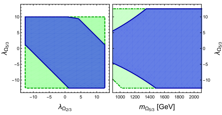
Figure 5: Allowed regions with 95 % C.L. of the parameter space of our LQ model from the experimental bounds on the Higgs boson multipliers $\kappa_{\gamma}$ and $\kappa_{g}$ for $m_{\Omega_{2/3}}=m_{\Omega_{5/3}}$. The left plot shows the allowed region in the $\lambda_{\Omega_{5/3}}$ vs $\lambda_{\Omega_{2/3}}$ plane for three values of $m_{\Omega_{5/3}}$: 1000 GeV (solid-line boundary), and 1500 GeV (dashed-line boundary). The right plot shows the allowed area in the $\lambda_{\Omega_{5/3}}$ vs $m_{\Omega_{5/3}}$ plane in the following scenarios of $\lambda_{\Omega_{2/3}}$: $\lambda_{\Omega_{2/3}}=\lambda_{\Omega_{5/3}}$ (solid-line boundary) and $\lambda_{\Omega_{2/3}}=-\lambda_{\Omega_{5/3}}$ (dot-dashed-line boundary). The vertical and horizontal lines correspond to the bounds from perturbativity $|\lambda_{\Omega_{2/3,\,5/3}}|\leq 4\pi$.

In summary the $\kappa_{\gamma}$ and $\kappa_{g}$ constraints are satisfied for $\lambda_{\Omega_{5/3}}$ of the order of $O(10)$, with the largest values allowed for a heavy LQ. In our analysis below we will use however the conservative value $\lambda_{\Omega_{5/3}}\simeq 1$ as a very large value would violate the perturbativity of the LQ coupling.

5.3 Constraints from the muon anomalous magnetic moment and the LFV decay $\tau\to\mu\gamma$

The experimental bounds on the muon anomalous magnetic dipole moment (MDM) $a_{\mu}$ and the LFV tau decays provide an useful tool to constrain LFV effects Tanabashi:2018oca . In particular, $a_{\mu}$ can be useful to constrain the LQ couplings $\lambda^{\mu u_{i}}_{L,R}$ ($u_{i}=c,t$), whereas the decay $\tau\to\mu\gamma$ allow us to constrain the $\lambda^{\tau u_{i}}_{L,R}$ ones.

5.3.1 Muon anomalous magnetic dipole moment

Currently there is a discrepancy between the experimental and theoretical values of the muon anomalous MDM $\Delta a_{\mu}=a_{\mu}^{\rm Theo.}-a_{\mu}^{\rm Exp.}=268\,(63)\,(43)\times 10^{-11}$ Tanabashi:2018oca . We assume that this discrepancy is due to the LQ contribution, though such a puzzle could be settled in the future once new experimental measurements and more accurate evaluations of the hadronic contributions were available.

The contribution of scalar LQs $\Omega_{5/3}$ to the muon anomalous magnetic dipole moment $a_{\mu}^{\rm LQ}$ arises at the one-loop level from the triangle diagrams of Fig. 2 with $f_{j}=f_{i}=\mu$ and $f_{k}=u_{k}$. It can be written as Bolanos:2013tda

$$a_{\mu}^{\rm LQ} =-\sum_{u_{k}=c,\,t}\frac{3\,\sqrt{x_{\mu}}}{32\pi^{2}}\Bigg{(}\sqrt{x_{\mu}}\left(\left|\lambda^{\mu u_{k}}_{L}\right|^{2}+\left|\lambda^{\mu u_{k}}_{R}\right|^{2}\right)F\left(x_{\mu},x_{u_{k}}\right)$$

$$+2\,\sqrt{x_{u_{k}}}\,{\rm Re}\left(\lambda^{\mu u_{k}}_{L}{\lambda^{\mu u_{k}}_{R}}^{*}\right)G\left(x_{\mu},x_{u_{k}}\right)\Bigg{)},$$ (35)

where $x_{a}=m_{a}^{2}/m^{2}_{\Omega_{5/3}}$. The $F(x,y)$ and $G(x,y)$ functions are presented in D in terms of Feynman parameter integrals and Passarino-Veltman scalar functions. Since $x_{\mu}\ll x_{u_{k}}$, we have the following approximate expression

$$a_{\mu}^{\rm LQ} \simeq-\sum_{u_{k}=c,\,t}\frac{3\,\sqrt{x_{\mu}}\sqrt{x_{u_{k}}}}{16\pi^{2}}\,{\rm Re}\left(\lambda^{\mu u_{k}}_{L}{\lambda^{\mu u_{k}}_{R}}^{*}\right)G\left(x_{\mu},x_{u_{k}}\right),$$ (36)

Since $\Omega_{2/3}$ is a chiral LQ, its contribution to $a_{\mu}$ is proportional to the muon mass and is thus subdominant. We now consider that the $\Delta a_{\mu}$ discrepancy is due to the LQ contribution $a_{\mu}^{\rm LQ}$ and show in Fig. 6 the allowed area in the ${\rm Re}\left(\lambda_{L}^{\mu c}\lambda_{R}^{\mu c}\right)$ vs ${\rm Re}\left(\lambda_{L}^{\mu t}\lambda_{R}^{\mu t}\right)$ plane for three values of $m_{\Omega_{5/3}}$. We note that a positive contribution from LQs to $a_{\mu}$ is required to explain the discrepancy, therefore there are three possible scenarios:

1. ${\rm Re}\left(\lambda_{L}^{\mu c}\lambda_{R}^{\mu c}\right)$ and ${\rm Re}\left(\lambda_{L}^{\mu t}\lambda_{R}^{\mu t}\right)<0$.

2. ${\rm Re}\left(\lambda_{L}^{\mu c}\lambda_{R}^{\mu c}\right)<0$ and ${\rm Re}\left(\lambda_{L}^{\mu t}\lambda_{R}^{\mu t}\right)>0$.

3. ${\rm Re}\left(\lambda_{L}^{\mu c}\lambda_{R}^{\mu c}\right)>0$ and ${\rm Re}\left(\lambda_{L}^{\mu t}\lambda_{R}^{\mu t}\right)<0$.

In the first scenario (left plot of Fig. 6) we observe that while ${\rm Re}\left(\lambda_{L}^{\mu c}\lambda_{R}^{\mu c}\right)$ can range between $10^{-4}$ and $10^{-3}$ for negligible ${\rm Re}\left(\lambda_{L}^{\mu c}\lambda_{R}^{\mu c}\right)$, the latter can range between $10^{-3}$ and $10^{-2}$ for negligible ${\rm Re}\left(\lambda_{L}^{\mu t}\lambda_{R}^{\mu t}\right)$, with the largest allowed values corresponding to heavy $m_{\Omega_{5/3}}$. On the other hand, more large values of the LQ couplings are allowed when ${\rm Re}\left(\lambda_{L}^{\mu c}\lambda_{R}^{\mu c}\right)$ and ${\rm Re}\left(\lambda_{L}^{\mu t}\lambda_{R}^{\mu t}\right)$ are of opposite sign (right plot) as there is a cancellation between the contributions of the $c$ and $t$ quarks. In particular, there is a very narrow band where ${\rm Re}\left(\lambda_{L}^{\mu c}\lambda_{R}^{\mu c}\right)\simeq O(10)$ and ${\rm Re}\left(\lambda_{L}^{\mu t}\lambda_{R}^{\mu t}\right)\simeq O(1)$.

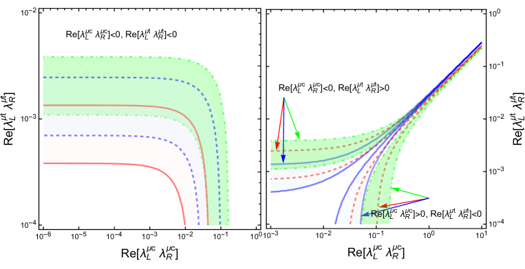
Figure 6: Allowed regions with 95 % C.L. of the parameter space of our LQ model assuming that the contributions of LQ $\Omega_{5/3}$ along with the $c$ and $t$ quarks are responsible for the muon anomalous MDM discrepancy $\Delta a_{\mu}$. We show the allowed region in the ${\rm Re}\left(\lambda_{L}^{\mu c}\lambda_{R}^{\mu c}\right)$ vs ${\rm Re}\left(\lambda_{L}^{\mu t}\lambda_{R}^{\mu t}\right)$ plane for two values of $m_{\Omega_{5/3}}$: 1000 GeV (solid-line boundary), 1500 GeV (dashed-line boundary), and 2000 GeV (dot-dashed-line boundary). In the left plot we assume that both ${\rm Re}\left(\lambda_{L}^{\mu c}\lambda_{R}^{\mu c}\right)<0$ and ${\rm Re}\left(\lambda_{L}^{\mu t}\lambda_{R}^{\mu t}\right)<0$, whereas in the right plot we consider that they are of opposite sign.

5.3.2 Decay $\tau\to\mu\gamma$

The LQ couplings $\lambda_{L,R}^{\tau u_{i}}$ and $\lambda_{L,R}^{\mu u_{i}}$ can be constrained by the experimental bound on the LFV tau decay $\tau\to\mu\gamma$, which can receive the contributions of loops with $\Omega_{5/3}$ accompanied by the up quarks. Such contributions follow straightforwardly from our result for the $f_{i}\to f_{j}\gamma$ decay width given in Eq. (3.1) after the proper replacements are made. The result is in agreement with previous calculations of the $\ell_{i}\to\ell_{j}\gamma$ decay width Bolanos:2013tda .

If the LQ couples to both the $c$ and $t$ quarks, the $\tau\to\mu\gamma$ decay width acquires the form

$$\Gamma(\tau\to\mu\gamma) \sim\Big{\|}\sum_{u_{i}=c,t}\left(\alpha_{LL}^{\mu u_{i}}\lambda_{L}^{\mu u_{i}}\lambda_{L}^{\tau u_{i}}+\alpha_{RR}^{\mu u_{i}}\lambda_{R}^{\mu u_{i}}\lambda_{R}^{\tau u_{i}}\right.$$

$$+\left.\alpha_{LR}^{\mu u_{i}}\lambda_{L}^{\mu u_{i}}\lambda_{R}^{\tau u_{i}}\right)\Big{\|}^{2}+\left(L\leftrightarrow R\right),$$ (37)

where $\alpha_{LL}^{\mu u_{i}}$, etc. stand for the loop integrals. To simplify our analysis we assume the scenario where $\lambda_{R}^{\ell u_{i}}/\lambda_{L}^{\ell u_{i}}=O(\epsilon)$ ($\ell=\mu,\,\tau$), with $\epsilon=10^{-3}$(predominantly left-handed couplings), $10^{-1}$ (small right handed-couplings), and 1 (purely scalar couplings). We do not analyze the case when $\epsilon>1$ as a similar situation is observed as in the $\epsilon<1$ case but with $\lambda_{L}^{\ell u_{i}}$ replaced by $\lambda_{R}^{\ell u_{i}}$. Thus the parameter $\epsilon$ is a measure of the relative size between the right and left-handed LQ couplings. Under this assumption, the $\tau\to\mu\gamma$ decay width becomes a function of the products $\lambda_{L}^{\mu c}\lambda_{L}^{\tau c}$ and $\lambda_{L}^{\mu t}\lambda_{L}^{\tau t}$. We thus show in Fig. 7 the allowed area in the $\lambda_{L}^{\mu c}\lambda_{L}^{\tau c}$ vs $\lambda_{L}^{\mu t}\lambda_{L}^{\tau t}$ plane for three values of $m_{\Omega_{5/3}}$. We observe that for $m_{\Omega_{5/3}}=1000$ GeV the largest allowed area is obtained in the scenario with $\epsilon=10^{-3}$, which allow $\lambda_{L}^{\mu u_{i}}\lambda_{L}^{\tau u_{i}}$ values as large as $O(10^{-1})$, whereas the smallest area is obtained when $\epsilon=1$, which allows $\lambda_{L}^{\mu u_{i}}\lambda_{L}^{\tau u_{i}}$ values of the order of $O(10^{-4})$. Such bounds are slightly relaxed when $m_{\Omega_{5/3}}$ increases up to 2 TeV.

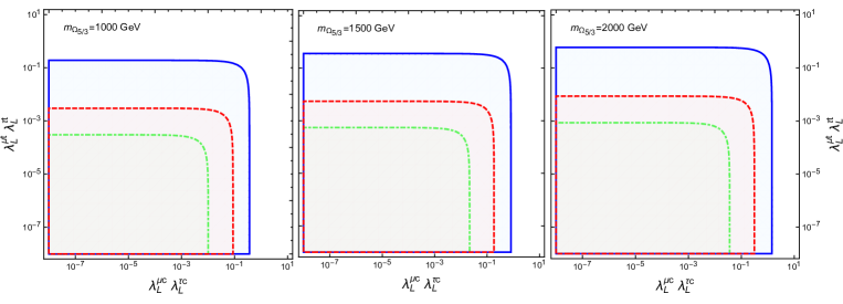
Figure 7: Allowed area with 95% C.L. in the $\lambda_{L}^{\mu c}\lambda_{L}^{\tau c}$ vs $\lambda_{L}^{\mu t}\lambda_{L}^{\tau t}$ plane from the experimental bound on the $\tau\to\mu\gamma$ decay for three values of $m_{\Omega_{5/3}}$ in the scenario with $\lambda_{R}^{\ell u_{i}}/\lambda_{L}^{\ell u_{i}}=O(\epsilon)$, for $\epsilon=10^{-3}$ (solid-line boundary), $\epsilon=0.1$ (dashed-line boundary), and $\epsilon=1$ (dot-dashed-line boundary).

As far as constraints on the $|\lambda_{L,R}^{\ell u_{i}}|$ couplings from direct LQ searches at the LHC via the Drell-Yan process Sirunyan:2018exx , single production Khachatryan:2015qda , and pair production Sirunyan:2018ryt , an up-to-date discussion is presented in Ref. Schmaltz:2018nls . A restricted scenario (minimal LQ model) is considered where each LQ is allowed to couple to just one lepton-quark pair. In particular, a 95% C.L. limit on $|\lambda^{\mu c}|$ of the order of $O(1)$ is obtained for a LQ with a mass above the 1 TeV level from the Drell-Yan process Sirunyan:2018exx , whereas the bounds obtained from the LHC Run 1 and Run 2 data on single production Khachatryan:2015qda yield less stringent bounds. Although such limit could be relaxed in a more general scenario where the LQ is allowed to couple to more than one fermion pair, below we assume a conservative scenario and consider the bound $|\lambda^{\mu c}|\leq O(1)$, whereas for the remaining couplings we impose the $|\lambda_{L,R}^{\mu t}|,\,|\lambda_{L,R}^{\tau u_{i}}|<4\pi$ bound to avoid the breakdown of perturbativity.

We are interested in the region of the parameter space where the largest $t\to cX$ and $t\to c\bar{\ell}\ell$ branching ratios can be reached, which is the area where either $\lambda_{L}^{\tau t}\lambda_{L}^{\tau c}$ or $\lambda_{L}^{\mu t}\lambda_{L}^{\mu c}$ reaches their largest allowed values. Again we consider the scenario with $\lambda_{R}^{\ell u_{i}}/\lambda_{L}^{\ell u_{i}}=O(\epsilon)$, with four $\epsilon$ values, and perform a scan of $(\lambda_{L}^{\mu c},\,\lambda_{L}^{\mu t},\,\lambda_{L}^{\tau c},\,\lambda_{L}^{\tau t})$ points consistent with both the $\Delta a_{\mu}$ discrepancy (Fig. 6) and the constraint on the $\tau\to\mu\gamma$ decay (Fig. 7) for two values of $m_{\Omega_{5/3}}$: we consider a large mass splitting to observe how the LQ couplings get constrained by the experimental data. As already discussed, we also impose the bound $|\lambda_{L,R}^{\mu c}|\leq O(1)$ from the direct LQ search at the LHC and, to avoid perturbativity violation, we impose the extra constraint $|\lambda_{L,R}^{\mu t}|,\,|\lambda_{L,R}^{\tau u_{i}}|<4\pi$. The corresponding allowed areas in the $\lambda_{L}^{\mu t}\lambda_{L}^{\mu c}$ vs $\lambda_{L}^{\tau t}\lambda_{L}^{\tau c}$ plane are shown in Fig. 8. We observe that, for $m_{\Omega_{5/3}}=1000$ GeV, the scenario with $\epsilon=10^{-3}$ (top left plot) allows values of $\lambda_{L}^{\tau c}\lambda_{L}^{\tau t}$ as large as $O(1)$ for $\lambda_{L}^{\mu t}\lambda_{L}^{\mu c}$ of the order of $10^{-1}$, but values of the order of the order of $O(1)$ are allowed for $\lambda_{L}^{\mu c}\lambda_{L}^{\mu t}$ for $\lambda_{L}^{taut}\lambda_{L}^{\tau c}$ of the order of $10^{-2}$. For fixed $\epsilon$, the allowed area expands slightly when the LQ mass increases, which is expected as the loop functions become suppressed for large LQ mass, thereby allowing larger couplings. On the other hand, for fixed $m_{\Omega_{5/3}}$ GeV, the allowed areas shrink significantly in the $\lambda_{L}^{\mu t}\lambda_{L}^{\mu c}$ direction and slightly in the $\lambda_{L}^{\tau t}\lambda_{L}^{\tau c}$ direction as $\epsilon$ increases. For instance, in the scenario when $\epsilon=1$ (bottom right plot), the largest allowed $\lambda_{L}^{\mu t}\lambda_{L}^{\mu c}$ values for $m_{\Omega_{5/3}}=1000$ GeV are of the order of $O(10^{-3})$ for small $\lambda_{L}^{\tau t}\lambda_{L}^{\tau c}$, whereas the latter can be as large as $O(10^{-1})$ for very small $\lambda_{L}^{\mu t}\lambda_{L}^{\mu c}$. We conclude that the scenario with predominantly dominant left-handed couplings ($\epsilon=10^{-3}$) is the one that allows the largest values of the LQ couplings.

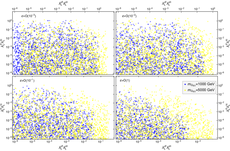
Figure 8: Allowed areas with 95% C.L. in the $\lambda_{L}^{\mu t}\lambda_{L}^{\mu c}$ vs $\lambda_{L}^{\tau t}\lambda_{L}^{\tau c}$ plane consistent with both the $\Delta a_{\mu}$ discrepancy and the experimental bound on the $\tau\to\mu\gamma$ decay for $m_{\Omega_{5/3}}=1000$ (dark points) and 5000 GeV (light points) in the scenarios where $\lambda_{R}^{\ell u_{i}}/\lambda_{L}^{\ell u_{i}}=O(\epsilon)$, for four $\epsilon$ values. For the $\lambda^{\mu c}$ coupling we use the constraint $|\lambda^{\mu c}|\leq O(1)$ from direct searches at the LCH Schmaltz:2018nls , whereas for the remaining couplings we use the additional constraint $|\lambda_{L,R}^{\ell u_{i}}|\leq 4\pi$ to avoid perturbativity violation. Here $\ell=\mu,\,\tau$ and $u_{i}=c,\,t$.

6 Numerical analysis of the $t\to cX$ and $t\to c\bar{\ell}\ell$ branching ratios

We now turn to analyze the behavior of the $t\to cX$ and $t\to c\bar{\ell}\ell$ branching ratios in the allowed area of the parameter space. For the numerical evaluation of the one-loop induced decays $t\to cX$ we have made a cross-check by evaluating the Passarino-Veltman scalar functions via the LoopTools package vanOldenborgh:1989wn ; Hahn:1998yk and then comparing the results with those obtained by numerical integration of the parametric integrals. For the tree-level induced decay $t\to c\bar{\ell}\ell$ we have used the Mathematica numerical integration routines to solve the two-dimensional integral of Eq. (22).

6.1 $t\to cX$ branching ratios

We first consider two $\epsilon$ values and present in Table 1 a few sets of allowed $(\lambda_{L}^{\mu c}$, $\lambda_{L}^{\mu t}$, $\lambda_{L}^{\tau c}$, $\lambda_{L}^{\tau t})$ points where the $t\to cX$ decays can reach their largest branching ratios for three LQ masses. In the scenario where $\epsilon=10^{-3}$ we observe that there is a small area where all of the $t\to cX$ branching ratios can be as large as $10^{-9}-10^{-8}$ for $m_{\Omega_{5/3}}=1000$ GeV, though they get suppressed by one order of magnitude when $m_{\Omega_{5/3}}$ increases up to 2000 GeV. In such an area, the LQ couplings $\lambda_{L}^{\mu u_{i}}$ are rather small, whereas the $\lambda_{L}^{\tau t}$ one is very close to the perturbative limit, which means that this possibility would require a large amount of fine-tuning. As for the $\epsilon=10^{-1}$ scenario, we observe that the $t\to cX$ branching ratios are much smaller than in the $\epsilon=10^{-3}$ scenario: they can be of the order of $10^{-9}-10^{-10}$ at most for $m_{\Omega_{5/3}}=1000$ GeV, and decrease by one order of magnitude as $m_{\Omega_{5/3}}$ increases up to 2000 GeV. We refrain from presenting the results for the $\epsilon=1$ scenario as the $t\to cX$ branching ratios are two orders of magnitude than in the $\epsilon=10^{-3}$ scenario.

We also observe in Table 1 that all the branching ratios ${\rm Br}(t\to cX)$ are of similar order of magnitude, with ${\rm Br}(t\to cZ)$ slightly larger. It seems surprising that ${\rm Br}(t\to cg)$ is about the same size than ${\rm Br}(t\to c\gamma)$, whereas in the SM and other of its extensions it is one or two orders of magnitude larger. To explain this result, let us examine the case of the SM, where the $t\to c\gamma$ decay proceeds via a Feynman diagram where the photon emerges off a down-type quark and so the squared amplitude for the analogue $t\to cg$ diagram has an enhancement factor of $c_{F}\left[g_{S}/(-1/3e)\right]^{2}\simeq O(10^{2})$, where $c_{F}=4/3$ is the color factor. On the other hand, in our LQ model the photon emerges off the charge $5/3e$ LQ, which means that the enhancement factor for the squared $t\to cg$ amplitude is just $c_{F}\left[g_{S}/(5/3e)\right]^{2}\simeq O(1)$. Furthermore, in our LQ model the Feynman diagram where the photon emerges off the LQ gives a smaller contribution than that where it emerges off the lepton, which is absent in the $t\to cg$ decay. These two facts conspire to yield ${\rm Br}(t\to cg)\gtrsim{\rm Br}(t\to c\gamma)$. It is also worth mentioning that the $t\to cH$ decay receives its main contribution from the diagram where the Higgs boson is emitted off the LQ line, and thus its decay width is very sensitive to the magnitude of the $\lambda_{\Omega_{5/3}}$ coupling.

Table 1: Branching ratios of the $t\to cX$ decays for a few $(\lambda_{L}^{\mu c},\lambda_{L}^{\mu t},\lambda_{L}^{\tau c}\lambda_{L}^{\tau t})$ points inside the area allowed by the $\Delta a_{\mu}$ discrepancy and the experimental bound on the $\tau\to\mu\gamma$ decay. We consider the scenario where $\lambda_{R}^{\ell u}/\lambda_{L}^{\ell u_{i}}=O(\epsilon)$ for $\epsilon=10^{-3}$ and $10^{-1}$. For the coupling of the Higgs boson to a LQ pair we use $\lambda_{\Omega_{5/3}}=1$. The $t\to cX$ branching ratios are given in units of $10^{-8}$ for $\epsilon=10^{-3}$ and $10^{-9}$ for $\epsilon=10^{-1}$.

$\lambda_{R}^{\ell u}/\lambda_{L}^{\ell u_{i}}=O(10^{-3})$
$m_{\Omega_{5/3}}$ [GeV]	$\lambda_{L}^{\mu c}$	$\lambda_{L}^{\mu t}$	$\lambda_{L}^{\tau c}$	$\lambda_{L}^{\tau t}$	$\gamma$	$g$	$Z$	$H$
1000	$2.54\times 10^{-4}$	$7.8\times 10^{-1}$	$2.39\times 10^{-1}$	$9.48$	$0.416$	$0.665$	$1.02$	$0.68$
	$1.48\times 10^{-4}$	$6.54\times 10^{-1}$	$2.06\times 10^{-1}$	$7.87$	$0.212$	$0.339$	$0.521$	$0.347$
	$2.52\times 10^{-5}$	$1.02$	$1.72\times 10^{-1}$	$7.86$	$0.147$	$0.236$	$0.362$	$0.241$
	$1.25\times 10^{-5}$	$7.68\times 10^{-1}$	$1.28\times 10^{-1}$	$9.97$	$0.132$	$0.212$	$0.325$	$0.216$
	$8.47\times 10^{-5}$	$6.48\times 10^{-1}$	$2.54\times 10^{-1}$	$4.97$	$0.129$	$0.207$	$0.318$	$0.211$
1500	$1.31\times 10^{-3}$	$1.$	$3.49\times 10^{-1}$	$6.52$	$0.0819$	$0.131$	$0.246$	$0.135$
	$3.45\times 10^{-4}$	$9.21\times 10^{-1}$	$2.56\times 10^{-1}$	$8.46$	$0.0741$	$0.119$	$0.222$	$0.122$
	$1.02\times 10^{-5}$	$1.04$	$2.58\times 10^{-1}$	$8.04$	$0.0678$	$0.109$	$0.203$	$0.111$
	$2.17\times 10^{-6}$	$1.21$	$2.89\times 10^{-1}$	$6.89$	$0.0624$	$0.1$	$0.187$	$0.103$
	$1.65\times 10^{-4}$	$1.13$	$2.5\times 10^{-1}$	$6.84$	$0.0462$	$0.074$	$0.138$	$0.0758$
2000	$2.16\times 10^{-5}$	$1.1$	$4.48\times 10^{-1}$	$7.39$	$0.0543$	$0.0872$	$0.186$	$0.0894$
	$7.69\times 10^{-6}$	$1.29$	$3.29\times 10^{-1}$	$9.86$	$0.0524$	$0.0841$	$0.179$	$0.0862$
	$2.59\times 10^{-3}$	$1.07$	$3.69\times 10^{-1}$	$8.71$	$0.0512$	$0.082$	$0.175$	$0.0843$
	$6.09\times 10^{-3}$	$1.07$	$3.05\times 10^{-1}$	$8.34$	$0.0323$	$0.0514$	$0.111$	$0.0532$
	$3.9\times 10^{-4}$	$1.69$	$2.73\times 10^{-1}$	$8.98$	$0.0298$	$0.0478$	$0.102$	$0.049$
$\lambda_{R}^{\ell u}/\lambda_{L}^{\ell u_{i}}=O(10^{-1})$
$m_{\Omega_{5/3}}$ [GeV]	$\lambda_{L}^{\mu c}$	$\lambda_{L}^{\mu t}$	$\lambda_{L}^{\tau c}$	$\lambda_{L}^{\tau t}$	$\gamma$	$g$	$Z$	$H$
1000	$2.54\times 10^{-4}$	$7.8\times 10^{-1}$	$2.39\times 10^{-1}$	$9.48$	$4.51$	$6.73$	$10.2$	$6.92$
	$1.48\times 10^{-4}$	$6.54\times 10^{-1}$	$2.06\times 10^{-1}$	$7.87$	$2.3$	$3.43$	$5.21$	$3.53$
	$2.52\times 10^{-5}$	$1.02$	$1.72\times 10^{-1}$	$7.86$	$1.6$	$2.39$	$3.62$	$2.45$
	$1.25\times 10^{-5}$	$7.68\times 10^{-1}$	$1.28\times 10^{-1}$	$9.97$	$1.44$	$2.14$	$3.25$	$2.2$
	$8.47\times 10^{-5}$	$6.48\times 10^{-1}$	$2.54\times 10^{-1}$	$4.97$	$1.4$	$2.09$	$3.17$	$2.15$
1500	$1.31\times 10^{-3}$	$1.$	$3.49\times 10^{-1}$	$6.52$	$0.893$	$1.33$	$2.45$	$1.37$
	$3.45\times 10^{-4}$	$9.21\times 10^{-1}$	$2.56\times 10^{-1}$	$8.46$	$0.809$	$1.2$	$2.22$	$1.24$
	$1.02\times 10^{-5}$	$1.04$	$2.58\times 10^{-1}$	$8.04$	$0.739$	$1.1$	$2.03$	$1.13$
	$2.17\times 10^{-6}$	$1.21$	$2.89\times 10^{-1}$	$6.89$	$0.681$	$1.01$	$1.87$	$1.04$
	$1.65\times 10^{-4}$	$1.13$	$2.5\times 10^{-1}$	$6.84$	$0.504$	$0.749$	$1.38$	$0.772$
2000	$2.16\times 10^{-5}$	$1.1$	$4.48\times 10^{-1}$	$7.39$	$0.595$	$0.883$	$1.86$	$0.911$
	$7.69\times 10^{-6}$	$1.29$	$3.29\times 10^{-1}$	$9.86$	$0.574$	$0.851$	$1.79$	$0.878$
	$2.59\times 10^{-3}$	$1.07$	$3.69\times 10^{-1}$	$8.71$	$0.561$	$0.83$	$1.75$	$0.859$
	$6.09\times 10^{-3}$	$1.07$	$3.05\times 10^{-1}$	$8.34$	$0.354$	$0.52$	$1.11$	$0.542$
	$3.9\times 10^{-4}$	$1.69$	$2.73\times 10^{-1}$	$8.98$	$0.326$	$0.484$	$1.02$	$0.5$

Finally we show in Fig. 9 the contours of the $t\to cX$ branching ratios in the allowed area of the $\lambda_{L}^{\mu t}\lambda_{L}^{\mu c}$ vs $\lambda_{L}^{\tau t}\lambda_{L}^{\tau c}$ plane in the scenario with $\lambda_{R}^{\ell u_{i}}/\lambda_{L}^{\ell u_{i}}=O(10^{-3})$, where the largest values of the $t\to cX$ branching ratios are reached. As already noted, when $m_{\Omega_{5/3}}=1000$ GeV the largest $t\to cX$ branching ratios, of the order of $10^{-9}-10^{-8}$, are obtained in a tiny area where $\lambda_{L}^{\mu t}\lambda_{L}^{\mu c}$ is very small and $\lambda_{L}^{\tau t}\lambda_{L}^{\tau c}$ reaches its largest allowed values (top-left corner of the upper plots), but they decrease as the allowed area expands. It means that the largest branching ratios are obtained in the region where the main contribution arises from the loops with an internal tau lepton, which is due to the fact that the LQ couplings to the tau lepton are less constrained than those to the muon. We also observe that the $t\to cX$ branching ratios decrease by one or two orders of magnitude as $m_{\Omega_{5/3}}$ reaches the 2 TeV level, where they can be as large as $10^{-9}-10^{-10}$. The behavior of the $t\to cX$ branching ratios in the scenarios with $\epsilon=10^{-1}$ and $\epsilon=1$ is rather similar to that observed in Fig. 9, but they are one or two orders of magnitude below: they can only be as large as $10^{-9}$ for $\epsilon=10^{-1}$ and $10^{-10}$ for $\epsilon=1$.

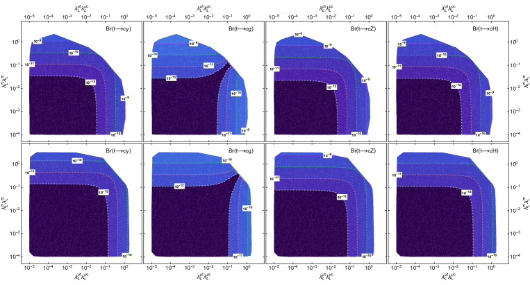
Figure 9: Contours of the branching ratios of the $t\to cX$ decays for $m_{\Omega_{5/3}}=1000$ (top plots) and 2000 GeV (bottom plots) in the $\lambda_{L}^{\mu t}\lambda_{L}^{\mu c}$ vs $\lambda_{L}^{\tau t}\lambda_{L}^{\tau c}$ plane for $(\lambda_{L}^{\mu c},\lambda_{L}^{\mu t},\lambda_{L}^{\tau c}\lambda_{L}^{\tau t})$ values inside the area allowed by the $\Delta a_{\mu}$ discrepancy and the experimental bound on the $\tau\to\mu\gamma$ in the scenario with $\lambda_{R}^{\ell u}/\lambda_{L}^{\ell u_{i}}=O(10^{-3})$.

6.2 $t\to c\bar{\ell}\ell$ branching ratios

We now perform the corresponding analysis for the $t\to c\bar{\ell}\ell$ ($\ell=\mu,\,\tau$) branching ratios in the area allowed by the experimental constraints discussed above. In Fig. 10 we show the contours of ${\rm Br}(t\to c\bar{\ell}\ell)$ in the $\lambda_{L}^{\ell t}$ vs $\lambda_{L}^{\ell c}$ plane in the scenario with $\lambda_{R}^{\ell u_{i}}/\lambda_{L}^{\ell u_{i}}=O(10^{-3})$ for two values of the LQ mass. We observe that for $m_{\Omega_{5/3}}=1000$ GeV, ${\rm Br}(t\to c\bar{\tau}\tau)$ can be of as large as $10^{-6}$, whereas ${\rm Br}(t\to c\bar{\mu}\mu)$ is one order of magnitude below, which is due to the fact that the $\lambda_{L}^{\mu q}$ couplings are more constrained than the $\lambda_{L}^{\tau q}$ ones. When $m_{\Omega_{5/3}}$ increases up to 2000 GeV, the $t\to c\bar{\ell}\ell$ branching ratios decrease by about one order of magnitude. As for the $t\to c\bar{\mu}\tau$ decay, its branching ratio is also suppressed as involves the $\lambda_{L}^{\mu q}$ couplings. In conclusion, the three-body tree-level decay $t\to c\bar{\ell}\ell$ can have larger branching ratios than the two-body one-loop decays $t\to cX$.

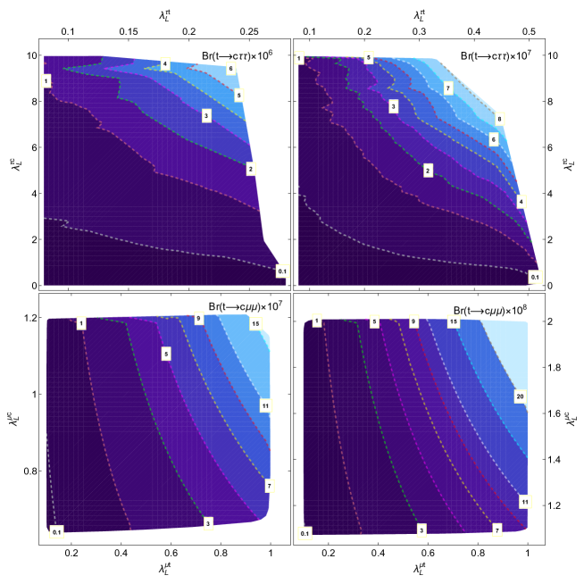
Figure 10: Contours of the branching ratios of the $t\to c\bar{\tau}\tau$ and $t\to c\bar{\mu}\mu$ decays for $m_{\Omega_{5/3}}=1000$ GeV (left plots) and 2000 GeV (right plots) in the $\lambda_{L}^{\ell t}$ vs $\lambda_{L}^{\ell c}$ plane for $(\lambda_{L}^{\mu c},\lambda_{L}^{\mu t},\lambda_{L}^{\tau c}\lambda_{L}^{\tau t})$ values inside the area allowed by the $\Delta a_{\mu}$ discrepancy and the experimental bound on the $\tau\to\mu\gamma$ in the scenario with $\lambda_{R}^{\ell u}/\lambda_{L}^{\ell u_{i}}=O(10^{-3})$.

7 Summary and outlook

The FCNC decays of the top quark $t\to cX$ ($X=\gamma,\,g,\,Z,\,H$) and $t\to c\bar{\ell}\ell$ ($\ell=\mu,\,\tau$) were calculated in a simple LQ model with no proton decay, where the SM is augmented by a $SU(2)$ scalar LQ doublet with hypercharge $Y=7/6$. In such a model there is a non-chiral LQ with electric charge $Q=5/3e$ that couples to charged leptons and up quarks and contribute to the FCNC decays of the top quark.

As far as the analytical results are concerned, we perform a general calculation of the FCNC fermion decays $f_{i}\to f_{j}X$ and $f_{i}\to f_{j}\bar{f}_{m}f_{l}$. The loop amplitudes of the $f_{i}\to f_{j}X$ decays are presented in terms of both Passarino-Veltman scalar functions and Feynman parameter integrals, which can be useful to calculate the contributions of other scalar LQs. On the other hand, an analytical expression is presented for the $f_{i}\to f_{j}\bar{f}_{m}f_{l}$ decay width, which can be numerically evaluated.

As for the numerical analysis, to obtain bounds on the parameter space of the model we assumed that the LQ only couples to the fermions of the last two families and used the experimental constraints on the LHC Higgs boson data, the muon anomalous magnetic dipole moment $a_{\mu}$, the LFV decay of the tau lepton $\tau\to\mu\gamma$, as well as the direct LQ searches at the LHC via the Drell-Yan process, single production, and double production. For the LQ couplings to charged leptons and up quarks $\lambda_{L,R}^{\ell u_{i}}$, a scenario was considered where $\lambda_{R}^{\ell u}/\lambda_{L}^{\ell u_{i}}=O(\epsilon)$, with $\epsilon$ being a measure of the relative size between the right- and left-handed LQ couplings. Afterwards, the $t\to cX$ and $t\to c\bar{\ell}\ell$ branching ratios were evaluated in the allowed region of the parameter space. In particular, we find that in the scenario where the LQ couplings are predominantly left-handed, $\epsilon=O(10^{-3})$, there is a tiny region of the parameter space where the branching ratios of the one-loop induced $t\to cX$ decay can be as large as $10^{-8}$ for $m_{\Omega_{5/3}}=1000$ GeV, with the main contribution arising from the loops with an internal tau lepton, although a large amount of fine-tuning between the LQ couplings would be required. However, for $\epsilon=10^{-1}$ ($\epsilon=1$), the main part of the allowed region yields $t\to cX$ branching ratios of the order of $10^{-9}$ ($10^{-10}$) at most. For $m_{\Omega_{5/3}}\geq 2000$ GeV, the largest $t\to cX$ branching ratios are of the order of $10^{-10}$ in all the scenarios analyzed in this work. Although the $t\to cX$ branching ratios are larger in our LQ model than in the SM, such contributions would be out of the reach of detection in the near future. As for the tree-level induced decays $t\to c\bar{\ell}\ell$, the $t\to c\bar{\tau}\tau$ branching ratio can be as large as $10^{-6}$ for $m_{\Omega_{5/3}}=1000$ GeV in the scenario with $\epsilon=O(10^{-3})$, but ${\rm Br}(t\to c\bar{\mu}\mu)$ is one order of magnitude below. These branching ratios decrease by about one order of magnitude when the LQ mass increases up to 2000 GeV.

It is worth noting that experimental constraints on the LQ mass and couplings obtained from the direct search at the LHC are very stringent, but they rely on several assumptions and may be relaxed, which would yield a slight enhancement of the LQ contribution to the top quark FCNC top quark decays. The magnitude of the $t\to cX$ branching ratios is similar to that recently found for the contributions from a scalar LQ with charge $-1/3e$, which arises in a model with a scalar LQ singlet Kim:2018oih . We do not consider this scenario in our analysis as we are interested in LQ models where no further symmetries must be invoked to forbid the proton decay Arnold:2013cva .

Appendix A Loop integrals for the $f_{i}\to f_{j}V$ decay

We now present the contribution of the scalar LQ $S$ to the $f_{i}\to f_{j}V$ loop amplitudes. Although in these Appendices $S$ will stand for the $\Omega_{5/3}$ LQ, as already explained, our results are also valid for the contribution of any other scalar LQ.

A.1 Passarino-Veltman results

We first define the following sets of ultraviolet finite Passarino-Veltman scalar function combinations

$$\Delta_{0} =B_{0}(m_{Z}^{2},m_{k}^{2},m_{k}^{2})-B_{0}(m_{j}^{2},m_{k}^{2},m_{S}^{2}),$$ (38)

$$\Delta_{1} =B_{0}(m_{Z}^{2},m_{k}^{2},m_{k}^{2})-B_{0}(0,m_{k}^{2},m_{S}^{2}),$$ (39)

$$\Delta_{2} =B_{0}(m_{i}^{2},m_{k}^{2},m_{S}^{2})-B_{0}(m_{j}^{2},m_{k}^{2},m_{S}^{2}),$$ (40)

$$\Delta_{3} =B_{0}(m_{j}^{2},m_{k}^{2},m_{S}^{2})-B_{0}(0,m_{k}^{2},m_{S}^{2}),$$ (41)

$$\Delta_{4} =B_{0}(0,m_{k}^{2},m_{k}^{2})-B_{0}(0,m_{S}^{2},m_{S}^{2}),$$ (42)

$$\Delta_{5} =B_{0}(0,m_{S}^{2},m_{S}^{2})-B_{0}(0,m_{k}^{2},m_{S}^{2}),$$ (43)

$$C_{kSk} =m_{S}^{2}C_{0}(m_{i}^{2},m_{j}^{2},0,m_{k}^{2},m_{S}^{2},m_{k}^{2}),$$ (44)

$$C_{SkS} =m_{S}^{2}C_{0}(m_{i}^{2},m_{j}^{2},0,m_{S}^{2},m_{k}^{2},m_{S}^{2}),$$ (45)

$$C_{ZkSk} =m_{S}^{2}C_{0}(m_{i}^{2},m_{j}^{2},m_{Z}^{2},m_{k}^{2},m_{S}^{2},m_{k}^{2}),$$ (46)

$$C_{ZSkS} =m_{S}^{2}C_{0}(m_{i}^{2},m_{j}^{2},m_{Z}^{2},m_{S}^{2},m_{k}^{2},m_{S}^{2}).$$ (47)

The form factors of Eq. (14) are given in terms of these ultraviolet-finite functions as follows.

A.1.1 $f_{i}\to f_{j}\gamma$ decay

There are only dipole form factors as the monopole ones must vanish due to electromagnetic gauge invariance. Although each Feynman diagram has ultraviolet divergences, they cancel out when summing over all the contributions. The results read

$$L^{\gamma} =\frac{N_{c}e}{16\pi^{2}}\frac{\sqrt{x_{i}}\xi_{ij}}{8}\Bigg{(}\frac{\lambda_{L}^{{ik}}\lambda_{L}^{{kj}}}{\sqrt{x_{i}}}\Big{(}x_{i}(Q_{S}-Q_{k})+\frac{1}{\xi_{ij}}\left(Q_{S}\left(x_{i}\left(x_{j}-2\xi_{k}\right)+x_{j}\xi_{k}\right)-Q_{k}\left(x_{i}\left(x_{j}+2\xi_{k}\right)-x_{j}\xi_{k}\right)\right)\Delta_{2}$$

$$-\xi_{k}\left(Q_{k}+Q_{S}\right)\Delta_{3}-2x_{i}\left(Q_{k}x_{k}C_{{kSk}}-Q_{S}C_{{SkS}}\right)\Big{)}+\frac{\lambda_{R}^{{ik}}\lambda_{R}^{{kj}}}{\sqrt{x_{j}}}\Big{(}\frac{x_{j}}{\xi_{ij}}\left(Q_{k}\left(\xi_{k}+x_{i}\right)+Q_{S}\left(\xi_{k}-x_{i}\right)\right)\Delta_{2}$$

$$+2\xi_{k}\left(Q_{k}+Q_{S}\right)\Delta_{3}+2x_{j}\left(Q_{k}x_{k}C_{{kSk}}-Q_{S}C_{{SkS}}\right)+x_{j}(Q_{k}-Q_{S})\Big{)}-\frac{\sqrt{x_{k}}\lambda_{L}^{{kj}}\lambda_{R}^{{ik}}}{\xi_{ij}^{3}}\Big{(}\xi_{{ij}}\left(Q_{k}+Q_{S}\right)\Delta_{2}$$

$$+Q_{k}\left(x_{j}^{2}-x_{i}\left(\eta_{{jk}}+\xi_{{jk}}\right)+x_{i}^{2}\right)C_{{kSk}}\Big{)}\Bigg{)},$$ (48)

where $N_{c}$ is the color number of the internal fermion and we introduced the following definitions $x_{a}=m_{a}^{2}/m_{S}^{2}$, $\xi_{ab}=x_{a}-x_{b}$, $\eta_{ab}=x_{a}+x_{b}$, $\xi_{a}=x_{a}-1$, and $\eta_{a}=x_{a}+1$. In addition, the right handed form factors can be obtained from the left-handed ones as follows

$$R^{\gamma}=L^{\gamma}\left(\lambda^{lm}_{L}\leftrightarrow\lambda^{lm}_{R},Q_{S}\to-Q_{S}\right).$$ (49)

A.1.2 $f_{i}\to f_{j}Z$ decay

The amplitude for this decay contains both dipole and monopole form factors. Again the ultraviolet divergences cancel when summing over partial contributions. The $L^{Z}$ and $L^{{}^{\prime}Z}$ form factors are too lengthy and can be written as a sum of partial terms arising from each contributing diagram as follows

$$L^{Z}=\frac{N_{c}g}{32\pi^{2}c_{W}}\frac{\sqrt{x_{i}}}{8}\sum_{j={\rm a,b}}\sum_{i=1}^{3}L^{\rm(j)}_{i},$$ (50)

and

$$L^{{}^{\prime}Z}=\frac{N_{c}g}{32\pi^{2}c_{W}}\frac{\sqrt{x_{i}}}{8}\sum_{j={\rm a,b,cd}}\sum_{i=1}^{3}L^{{}^{\prime}\rm(j)}_{i},$$ (51)

where the superscript stands for the Feynman diagram of Fig. 2 out of which the corresponding term arises, with (cd) standing for the sum of the contributions of diagrams (c) and (d).

The contributions of diagram (a) are given by

$$L_{1}^{(\rm a)} =\frac{\sqrt{x_{j}}g_{R}^{k}\lambda_{R}^{{ik}}\lambda_{R}^{{kj}}}{2\delta^{2}}\Bigg{(}\Big{(}x_{Z}^{3}+x_{Z}^{2}\left(4x_{i}-2x_{j}-6{\xi_{k}}\right)-\xi_{{ij}}x_{Z}\left(x_{j}+6{\xi_{k}}+5x_{i}\right)\Big{)}\Delta_{1}$$

$$+\Big{(}x_{Z}^{2}\left(\xi_{k}-5x_{i}\right)+2x_{Z}\left(2x_{i}\eta_{ij}+5x_{i}\xi_{k}-x_{j}\xi_{k}\right)+\xi_{{ij}}^{2}\left(\eta_{{ik}}-1\right)\Big{)}\Delta_{2}$$

$$+\frac{1}{x_{j}}\Big{(}x_{Z}^{3}\left(1-\eta_{{jk}}\right)+x_{Z}^{2}\left(x_{i}\left(3{\xi_{k}}-4x_{j}\right)+x_{j}\left(2x_{j}+7{\xi_{k}}\right)\right)$$

$$+\xi_{{ij}}x_{Z}\left(x_{i}\left(5x_{j}-3{\xi_{k}}\right)+x_{j}\left(x_{j}+5{\xi_{k}}\right)\right)+\xi_{{ij}}^{3}{\xi_{k}}\Big{)}\Delta_{3}$$

$$+2\Big{(}x_{Z}^{3}\left(\xi_{{ik}}+2\right)+x_{Z}^{2}\left(x_{i}\left(x_{j}-3x_{k}+2\right)+x_{j}\left(x_{k}-4\right)+3{\xi_{k}}^{2}-2x_{i}^{2}\right)$$

$$+\xi_{{ij}}x_{Z}\left(x_{i}\left(2x_{j}+3x_{k}-4\right)-x_{j}\left(x_{k}+2\right)+3{\xi_{k}}^{2}+x_{i}^{2}\right)+\xi_{{ij}}^{3}x_{k}\Big{)}C_{ZkSk}+\delta\left(\xi_{{ij}}+x_{Z}\right)\Bigg{)},$$ (52)

$$L_{2}^{(\rm a)} =\frac{g_{L}^{k}\lambda_{L}^{{ik}}\lambda_{L}^{{kj}}}{2\sqrt{x_{i}}\delta^{2}}\Bigg{(}x_{i}\Big{(}x_{Z}^{3}-2x_{Z}^{2}\left(3\xi_{k}-2x_{j}+x_{i}\right)+\xi_{{ij}}x_{Z}\left(5x_{j}+6\xi_{k}+x_{i}\right)\Big{)}\Delta_{1}$$

$$+\Big{(}x_{Z}^{3}\left(1-\eta_{{ik}}\right)\ +\left(x_{j}+2x_{i}\right)\left(3\xi_{k}+x_{i}\right)x_{Z}^{2}-x_{Z}\left(x_{i}^{2}\left(8x_{j}+3\xi_{k}\right)\right.$$

$$\left.-x_{i}x_{j}\left(x_{j}-2\xi_{k}\right)+3x_{j}^{2}\xi_{k}+x_{i}^{3}\right)-\xi_{{ij}}^{2}\left(x_{i}\left(x_{j}+2\xi_{k}\right)-x_{j}\xi_{k}\right)\Big{)}\Delta_{2}$$

$$+\Big{(}x_{Z}^{3}\left(1-\eta_{{ik}}\right)+x_{Z}^{2}\left(x_{i}\left(7\xi_{k}-4x_{j}\right)+3x_{j}\xi_{k}+2x_{i}^{2}\right)$$

$$-\xi_{{ij}}x_{Z}\left(x_{i}\left(5\eta_{{jk}}+x_{i}-5\right)-3x_{j}\xi_{k}\right)-\xi_{{ij}}^{3}\xi_{k}\Big{)}\Delta_{3}$$

$$+2x_{i}\Big{(}x_{Z}^{3}\left(\xi_{{jk}}+2\right)+x_{Z}^{2}\left(x_{j}\left(2-3x_{k}\right)-2x_{j}^{2}+x_{i}\left(\eta_{{jk}}-4\right)+3\xi_{k}^{2}\right)$$

$$-\xi_{{ij}}x_{Z}\left(\left(3x_{j}-x_{i}-6\right)x_{k}+\xi_{j}\left(x_{j}+2x_{i}-3\right)+3x_{k}^{2}\right)-\xi_{{ij}}^{3}x_{k}\Big{)}C_{ZkSk}+\delta x_{i}\left(x_{Z}-\xi_{{ij}}\right)\Bigg{)},$$ (53)

$$L_{3}^{{\rm(a)}} =\frac{\sqrt{x_{k}}\lambda_{L}^{{kj}}\lambda_{R}^{{ik}}}{\delta}\Bigg{(}g_{L}^{k}\bigg{(}\Big{(}x_{Z}-\xi_{{ij}}\Big{)}\Delta_{0}+\Big{(}\eta_{{ij}}-x_{Z}\Big{)}\Delta_{2}+\Big{(}\left(\xi_{{jk}}+1\right)x_{Z}+\xi_{{ij}}\left(\eta_{{jk}}-1\right)\Big{)}C_{{kSk}}\bigg{)}$$

$$+g_{R}^{k}\Bigg{(}\Big{(}x_{Z}+\xi_{{ij}}\Big{)}\Delta_{0}-2x_{i}\Delta_{2}+\Big{(}x_{Z}\left(x_{i}-\xi_{k}\right)+x_{j}\xi_{k}+x_{i}\left(\xi_{{jk}}-\xi_{i}\right)\Big{)}C_{{kSk}}\Bigg{)},$$ (54)

$$L_{1}^{{}^{\prime}(\rm a)} =\frac{g_{R}^{k}\lambda_{R}^{{ik}}\lambda_{R}^{kj}}{2\delta^{2}}\Bigg{(}\Big{(}-x_{Z}^{4}+2x_{Z}^{3}\left(2\eta_{ij}-\xi_{k}\right)-x_{Z}^{2}\left(4x_{i}x_{j}+2\eta_{ij}\xi_{k}+5\xi_{ij}^{2}\right)+2\xi_{{ij}}^{2}x_{Z}\left(\eta_{{ij}}+2\xi_{k}\right)\Big{)}\Delta_{1}$$

$$+\Big{(}x_{Z}^{2}\left(x_{j}\xi_{k}-x_{i}\left(5(\eta_{j}-x_{k})+x_{i}\right)\right)+2\xi_{{ij}}x_{Z}\left(x_{j}\xi_{k}+x_{i}\left(2(1-\eta_{{jk}})+x_{i}\right)\right)-\xi_{{ij}}^{3}\left(\eta_{{ik}}-1\right)\Big{)}\Delta_{2}$$

$$+\Big{(}x_{Z}^{2}\left(2x_{i}\left(3\xi_{k}-5x_{j}\right)-x_{j}\left(x_{j}-6\xi_{k}\right)-x_{i}^{2}\right)+2\xi_{{ij}}^{2}x_{Z}\left(\eta_{{ij}}-3\xi_{k}\right)-\xi_{{ij}}^{4}\Big{)}\Delta_{3}$$

$$+2\Big{(}x_{Z}^{3}\left(2\eta_{ij}-\eta_{{ij}}x_{k}+x_{i}x_{j}+\xi_{k}^{2}\right)+x_{Z}^{2}\left(x_{i}\left(x_{j}\left(4-6x_{k}\right)+x_{j}^{2}+\xi_{k}^{2}\right)+x_{j}\left(x_{j}\left(x_{k}-4\right)+\xi_{k}^{2}\right)\right.$$

$$\left.+x_{i}^{2}\left(\eta_{{jk}}-4\right)\right)+\xi_{{ij}}^{2}x_{Z}\left(x_{j}\left(x_{k}+2\right)+x_{i}\left(x_{k}-2\xi_{j}\right)-2\xi_{k}^{2}\right)-\xi_{{ij}}^{4}x_{k}\Big{)}C_{ZkSk}+\delta x_{Z}\left(x_{Z}-\eta_{{ij}}\right)-\delta^{2}B_{{kS}}\Bigg{)}$$

$$+g_{L}^{k}\lambda_{R}^{{ik}}\lambda_{R}^{{kj}}x_{k}C_{ZkSk},$$ (55)

$$L_{2}^{{}^{\prime}(\rm a)} =\frac{g_{L}^{k}\lambda_{L}^{{ik}}\lambda_{L}^{{kj}}}{2\sqrt{x_{i}}\sqrt{x_{j}}\delta^{2}}\Bigg{(}2x_{i}x_{j}\delta x_{Z}+6x_{i}x_{j}\Big{(}x_{Z}^{3}-x_{Z}^{2}\left(\eta_{{ij}}+2\xi_{k}\right)\Big{)}\Delta_{1}-x_{j}\Big{(}x_{Z}^{3}\left(\xi_{k}+3x_{i}\right)$$

$$+x_{Z}^{2}\left(x_{i}\left(7(1-\eta_{{jk}})+x_{i}\right)-3x_{j}\xi_{k}\right)-\xi_{{ij}}x_{Z}\left(x_{i}\left(5x_{j}+7\xi_{k}\right)+3x_{j}\xi_{k}+5x_{i}^{2}\right)-\xi_{{ij}}^{3}\left(1-\eta_{{ik}}\right)\Big{)}\Delta_{2}$$

$$-\Big{(}x_{Z}^{3}\left(\eta_{{ij}}\xi_{k}+6x_{i}x_{j}\right)-x_{Z}^{2}\left(3x_{i}^{2}\left(2x_{j}+\xi_{k}\right)+2x_{i}x_{j}\left(3x_{j}+7\xi_{k}\right)+3x_{j}^{2}\xi_{k}\right)+3\eta_{{ij}}\xi_{{ij}}^{2}\xi_{k}x_{Z}-\xi_{{ij}}^{4}\xi_{k}\Big{)}\Delta_{3}$$

$$+2x_{i}x_{j}\Big{(}x_{Z}^{4}-2x_{Z}^{3}\left(\eta_{{ij}}+2x_{k}-3\right)+x_{Z}^{2}\left(2x_{i}x_{j}+2\eta_{ij}\left(x_{k}-3\right)+\eta_{ij}^{2}+6\xi_{k}^{2}\right)+2\xi_{{ij}}^{2}x_{k}x_{Z}\Big{)}C_{ZkSk}\Bigg{)},$$ (56)

$$L_{3}^{{}^{\prime}(\rm a)} =\frac{\sqrt{x_{k}}g_{L}^{k}}{\delta}\left(\sqrt{x_{i}}\lambda_{L}^{{ik}}\lambda_{R}^{{kj}}+\sqrt{x_{j}}\lambda_{L}^{{kj}}\lambda_{R}^{{ik}}\right)\Bigg{(}2x_{Z}\Delta_{0}-\Big{(}x_{Z}+\xi_{{ij}}\Big{)}\Delta_{2}+\Big{(}x_{Z}^{2}-x_{Z}\left(\eta_{{ij}}+2\xi_{k}\right)\Big{)}C_{ZkSk}\Bigg{)},$$ (57)

where $\delta=x_{i}^{2}-2(x_{j}+x_{Z})x_{i}+(x_{j}-x_{Z})^{2}$. The contributions of diagram (b) are

$$L_{1}^{(\rm b)} =\frac{g_{{VSS}}\sqrt{x_{j}}\lambda_{R}^{{ik}}\lambda_{R}^{{kj}}}{2\delta^{2}}\Bigg{(}\Big{(}-x_{Z}^{3}+2x_{Z}^{2}\left(x_{j}-3\xi_{k}-2x_{i}\right)+\xi_{{ij}}x_{Z}\left(x_{j}-6\xi_{k}+5x_{i}\right)\Big{)}\Delta_{1}$$

$$+\Big{(}x_{Z}^{2}\left(\xi_{k}+5x_{i}\right)-2x_{Z}\left(x_{i}\left(2\eta_{ij}-5\xi_{k}\right)+x_{j}\xi_{k}\right)-\xi_{{ij}}^{2}\left(\xi_{{ik}}+1\right)\Big{)}\Delta_{2}$$

$$+\frac{1}{x_{j}}\Big{(}x_{Z}^{3}\left(\xi_{{jk}}+1\right)+x_{Z}^{2}\left(x_{i}\left(4x_{j}+3\xi_{k}\right)+x_{j}\left(7\xi_{k}-2x_{j}\right)\right)$$

$$-\xi_{{ij}}x_{Z}\left(x_{j}\left(x_{j}-5\xi_{k}\right)+x_{i}\left(5x_{j}+3\xi_{k}\right)\right)+\xi_{{ij}}^{3}\xi_{k}\Big{)}\Delta_{3}-2\Big{(}x_{Z}^{3}\left(\xi_{k}+\eta_{ik}\right)$$

$$+x_{Z}^{2}\left(x_{i}\left(\xi_{j}+2(\xi_{k}-x_{i})\right)-x_{j}\left(4x_{k}-1\right)+3\xi_{k}^{2}\right)$$

$$-\xi_{{ij}}x_{Z}\left(2\left(x_{j}+2x_{i}\right)x_{k}+x_{j}-x_{i}\left(2x_{j}+x_{i}+3\right)-3\xi_{k}^{2}\right)+\xi_{{ij}}^{3}\Big{)}C_{ZSkS}-\delta\left(\xi_{{ij}}+x_{Z}\right)\Bigg{)},$$ (58)

$$L_{2}^{(\rm b)} =\frac{g_{{VSS}}\lambda_{L}^{{ik}}\lambda_{L}^{{kj}}}{2\sqrt{x_{i}}\delta^{2}}\Bigg{(}x_{i}\Big{(}-x_{Z}^{3}+2x_{Z}^{2}\left(x_{i}-2x_{j}-3{\xi_{k}}\right)+\xi_{{ij}}x_{Z}\left(6{\xi_{k}}-5x_{j}-x_{i}\right)\Big{)}\Delta_{1}$$

$$+\Big{(}x_{Z}^{3}\left(\xi_{{ik}}+1\right)+x_{Z}^{2}\left(x_{j}+2x_{i}\right)\left(3{\xi_{k}}-x_{i}\right)+x_{Z}\left(x_{i}^{2}\left(8x_{j}-3{\xi_{k}}\right)-x_{i}x_{j}\left(x_{j}+2{\xi_{k}}\right)-3x_{j}^{2}{\xi_{k}}+x_{i}^{3}\right)$$

$$+\xi_{{ij}}^{2}\left(x_{i}\left(x_{j}-2{\xi_{k}}\right)+x_{j}{\xi_{k}}\right)\Big{)}\Delta_{2}+\Big{(}x_{Z}^{3}\left(\xi_{{ik}}+1\right)+x_{Z}^{2}\left(x_{i}\left(4x_{j}+7{\xi_{k}}\right)+3x_{j}{\xi_{k}}-2x_{i}^{2}\right)$$

$$+\xi_{{ij}}x_{Z}\left(3x_{j}{\xi_{k}}+x_{i}\left(5\xi_{{jk}}+x_{i}+5\right)\right)-\xi_{{ij}}^{3}{\xi_{k}}\Big{)}\Delta_{3}-2x_{i}\Big{(}x_{Z}^{3}\left(\xi_{j}+2x_{k}\right)$$

$$-x_{Z}^{2}\left(x_{j}\left(3-2x_{k}\right)-x_{i}\left(\eta_{j}-4x_{k}\right)+2x_{j}^{2}-3{\xi_{k}}^{2}\right)$$

$$+x_{Z}\xi_{{ij}}\left(3-2\left(2x_{j}+x_{i}+3\right)x_{k}+x_{j}(x_{j}+2x_{i}+3)+3x_{k}^{2}-x_{i}\right)+\xi_{{ij}}^{3}\Big{)}C_{ZSkS}+x_{i}\delta\left(\xi_{{ij}}-x_{Z}\right)\Bigg{)},$$ (59)

$$L_{3}^{(\rm b)} =\frac{g_{{VSS}}\sqrt{x_{k}}\lambda_{L}^{{kj}}\lambda_{R}^{{ik}}}{\delta}\Bigg{(}2x_{Z}\Delta_{0}-\Big{(}x_{Z}+\xi_{{ij}}\Big{)}\Delta_{2}+\Big{(}x_{Z}^{2}+x_{Z}\left(2\xi_{k}-\eta_{{ij}}\right)\Big{)}C_{ZSkS}\Bigg{)},$$ (60)

$$L_{1}^{{}^{\prime}(\rm b)} =\frac{g_{{VSS}}\lambda_{R}^{{ik}}\lambda_{R}^{{kj}}}{2\delta^{2}}\Bigg{(}\Big{(}-x_{Z}^{4}+2x_{Z}^{3}\left(\eta_{{ij}}-\xi_{k}\right)-x_{Z}^{2}\left(2x_{i}\left(5x_{j}+\xi_{k}\right)+x_{j}\left(x_{j}+2\xi_{k}\right)+x_{i}^{2}\right)+4\xi_{{ij}}^{2}\xi_{k}x_{Z}\Big{)}\Delta_{1}$$

$$+\Big{(}2x_{i}x_{Z}^{3}+x_{Z}^{2}\left(x_{i}\left(3x_{j}+5\xi_{k}\right)+x_{j}\xi_{k}-5x_{i}^{2}\right)+2\xi_{{ij}}x_{Z}\left(x_{i}\left(3x_{j}-2\xi_{k}\right)+x_{j}\xi_{k}+2x_{i}^{2}\right)+\xi_{{ij}}^{3}\left(1-\eta_{{ik}}\right)\Big{)}\Delta_{2}$$

$$+\Big{(}2\eta_{{ij}}x_{Z}^{3}-x_{Z}^{2}\left(x_{j}\left(5x_{j}-6\xi_{k}\right)+x_{i}\left(6-6\eta_{{jk}}+5x_{i}\right)\right)+2\xi_{{ij}}^{2}x_{Z}\left(2\eta_{ij}-3\xi_{k}\right)-\xi_{{ij}}^{4}\Big{)}\Delta_{3}$$

$$+\Big{(}-2x_{k}x_{Z}^{4}+x_{Z}^{3}\left(2x_{k}\left(\eta_{{ij}}-x_{k}+2\right)+x_{i}\left(4-6x_{j}\right)+4x_{j}-2\right)+2x_{Z}^{2}\left(x_{i}^{2}\left(3x_{j}+x_{k}-4\right)\right.$$

$$\left.+x_{i}\left(x_{j}\left(4-6x_{k}\right)+3x_{j}^{2}-\xi_{k}^{2}\right)+x_{j}\left(x_{j}\left(x_{k}-4\right)-\xi_{k}^{2}\right)\right)+2\xi_{{ij}}^{2}x_{Z}\left(2\xi_{k}^{2}-\eta_{{ij}}\left(x_{k}-2\right)\right)\Big{)}C_{ZSkS}$$

$$+\delta x_{Z}\left(\eta_{{ij}}-x_{Z}\right)-\delta^{2}B_{{kS}}\Bigg{)},$$ (61)

$$L_{2}^{{}^{\prime}(\rm b)} =\frac{g_{{VSS}}\sqrt{x_{i}}\sqrt{x_{j}}\lambda_{L}^{{ik}}\lambda_{L}^{{kj}}}{\delta^{2}}\Bigg{(}\Big{(}-x_{Z}^{3}-x_{Z}^{2}\left(\eta_{{ij}}+6\xi_{k}\right)+2\xi_{{ij}}^{2}x_{Z}\Big{)}\Delta_{1}$$

$$+\frac{1}{2x_{i}}\Big{(}\left(\xi_{{ik}}+1\right)x_{Z}^{3}+x_{Z}^{2}\left(x_{i}\left(7\xi_{k}-x_{j}\right)+3x_{j}\xi_{k}+3x_{i}^{2}\right)+\xi_{{ij}}x_{Z}\left(x_{i}\left(x_{j}+7\xi_{k}\right)+3x_{j}\xi_{k}-3x_{i}^{2}\right)$$

$$+\xi_{{ij}}^{3}\left(1-\eta_{{ik}}\right)\Big{)}\Delta_{2}+\frac{1}{2x_{i}x_{j}}\Big{(}x_{Z}^{3}\left(2x_{i}x_{j}-\eta_{{ij}}\xi_{k}\right)+x_{Z}^{2}\left(x_{i}^{2}\left(2x_{j}+3\xi_{k}\right)+2x_{i}x_{j}\left(x_{j}+7\xi_{k}\right)+3x_{j}^{2}\xi_{k}\right)$$

$$-\xi_{{ij}}^{2}x_{Z}\left(3\eta_{{ij}}\xi_{k}+4x_{i}x_{j}\right)+\xi_{{ij}}^{4}\xi_{k}\Big{)}\Delta_{3}+\Big{(}x_{Z}^{3}\left(2-\eta_{{ij}}-4x_{k}\right)+2x_{Z}^{2}\left(\eta_{{ij}}\eta_{k}+x_{i}x_{j}+\xi_{ij}^{2}-3\xi_{k}^{2}\right)$$

$$+\xi_{{ij}}^{2}x_{Z}\left(2x_{k}-\eta_{{ij}}-4\right)\Big{)}C_{ZSkS}-\delta x_{Z}\Bigg{)},$$ (62)

$$L_{3}^{{}^{\prime}(\rm b)} =\frac{g_{{VSS}}\sqrt{x_{k}}}{\delta}\left(\sqrt{x_{i}}\lambda_{L}^{{ik}}\lambda_{R}^{{kj}}+\sqrt{x_{j}}\lambda_{L}^{{kj}}\lambda_{R}^{{ik}}\right)\Bigg{(}2x_{Z}\Delta_{0}-\Big{(}x_{Z}+\xi_{{ij}}\Big{)}\Delta_{2}+x_{Z}\Big{(}x_{Z}+2\xi_{k}-\eta_{{ij}}\Big{)}C_{ZSkS}\Bigg{)}.$$ (63)

Finally Feynman diagrams (c) and (d) only contribute to monopole terms. The corresponding contribution of both diagrams is

$$\sum_{i=1}^{3}L_{i}^{{}^{\prime}(\rm cd)} =\frac{g_{L}^{j}\lambda_{R}^{{ik}}\lambda_{R}^{{kj}}}{2\xi_{{ij}}}\Bigg{(}\Big{(}\eta_{{ik}}-1\Big{)}\Delta_{2}+\xi_{{ij}}\Delta_{3}-2x_{k}\Delta_{4}-2\xi_{k}\Delta_{5}+\xi_{{ij}}B_{{kS}}-2\xi_{k}\Bigg{)}$$

$$+\frac{g_{L}^{j}\lambda_{L}^{{ik}}\lambda_{L}^{{kj}}}{2\sqrt{x_{i}}\sqrt{x_{j}}}\Bigg{(}\frac{1}{\xi_{{ij}}}\left(\eta_{{ik}}-1\right)x_{j}\Delta_{2}-\xi_{k}\Delta_{3}\Bigg{)}+\frac{\sqrt{x_{k}}g_{L}^{j}}{\xi_{{ij}}}\left(\sqrt{x_{i}}\lambda_{L}^{{ik}}\lambda_{R}^{{kj}}+\sqrt{x_{j}}\lambda_{L}^{{kj}}\lambda_{R}^{{ik}}\right)\Delta_{2}.$$ (64)

We can observe that the ultraviolet divergent term $B_{kS}\equiv B_{0}(0,m_{k}^{2},m_{S}^{2})$, which appears only in the monopole terms, is canceled out when summing over all the contributions.

Furthermore, the form factors associated with the right-handed terms are given by

$$R^{Z}=L^{Z}\left(\lambda^{lm}_{L}\leftrightarrow\lambda^{lm}_{R},g_{ZSS}\to-g_{ZSS}\right),$$ (65)

and

$$R^{{}^{\prime}Z}=-L^{{}^{\prime}Z}\left(\lambda^{lm}_{L}\leftrightarrow\lambda^{lm}_{R},g_{ZSS}\to-g_{ZSS}\right).$$ (66)

A.2 Feynman parameter results

A.2.1 $f_{i}\to f_{j}\gamma$ decay

The $L^{\gamma}$ form factor of Eq. (14) is ultraviolet finite and is given in terms of Feynman parameter integrals as follows

$$L^{\gamma} =\frac{N_{c}g^{2}e\sqrt{x_{i}}}{62c_{W}^{2}\pi^{2}}\frac{1}{2}\int_{0}^{1}dx\int_{0}^{1-x}dy\Bigg{(}\frac{Q_{k}}{\zeta_{1}}\left(xy\sqrt{x_{i}}\lambda_{L}^{{ik}}\lambda_{L}^{{kj}}-\lambda_{R}^{{ik}}\left(x\sqrt{x_{j}}(x+y-1)\lambda_{R}^{{kj}}+(x-1)\sqrt{x_{k}}\lambda_{L}^{{kj}}\right)\right)$$

$$+\frac{Q_{S}}{\zeta_{2}}(x+y-1)\left(x\sqrt{x_{i}}\lambda_{L}^{{ik}}\lambda_{L}^{{kj}}+y\sqrt{x_{j}}\lambda_{R}^{{ik}}\lambda_{R}^{{kj}}+\sqrt{x_{k}}\lambda_{L}^{{kj}}\lambda_{R}^{{ik}}\right)\Bigg{)},$$ (67)

where

$$\zeta_{1} =x\left(y\xi_{ji}+x_{j}(x-1)-\xi_{k}\right)+x_{k},$$ (68)

$$\zeta_{2} =xy\eta_{ij}-x\left(\eta_{ik}-1\right)+x^{2}x_{i}-y\left(\eta_{jk}-yx_{j}\right)+x_{k}+y.$$ (69)

The $R^{\gamma}$ form factor is given by Eq. (49), whereas monopole terms $L^{{}^{\prime}\gamma}$ and $R{{}^{\prime}\gamma}$ are zero as already mentioned (one must consider electric charge conservation).

A.2.2 $f_{i}\to f_{j}Z$ decay

The dipole terms of Eq. (50), which only arise from diagrams (a) and (b), are ultraviolet finite and are given by

$$L^{\rm(a)}=\int_{0}^{1}dx\int_{0}^{1-x}dy\frac{1}{\zeta^{\prime}_{1}}\left(xy\sqrt{x_{i}}g_{L}^{k}\lambda_{L}^{{ik}}\lambda_{L}^{{kj}}-x\sqrt{x_{j}}(x+y-1)g_{R}^{k}\lambda_{R}^{{ik}}\lambda_{R}^{{kj}}+\sqrt{x_{k}}\lambda_{L}^{{kj}}\lambda_{R}^{{ik}}\left(yg_{L}^{k}-(x+y-1)g_{R}^{k}\right)\right),$$ (70)

$$L^{\rm(b)}=g_{{VSS}}\int_{0}^{1}dx\int_{0}^{1-x}dy\frac{(x+y-1)}{\zeta^{\prime}_{2}}\left(x\sqrt{x_{i}}\lambda_{L}^{{ik}}\lambda_{L}^{{kj}}+y\sqrt{x_{j}}\lambda_{R}^{{ik}}\lambda_{R}^{{kj}}+\sqrt{x_{k}}\lambda_{L}^{{kj}}\lambda_{R}^{{ik}}\right),$$ (71)

whereas the partial contributions to the monopole terms of Eq. (51) are ultraviolet divergent and read

$$L^{{}^{\prime}\rm(a)} =\int_{0}^{1}dx\int_{0}^{1-x}dy\frac{1}{\zeta^{\prime}_{1}}\Bigg{(}x(y-1)\sqrt{x_{i}}\sqrt{x_{j}}g_{L}^{k}\lambda_{L}^{{ik}}\lambda_{L}^{{kj}}+(y-1)\sqrt{x_{i}}\sqrt{x_{k}}g_{L}^{k}\lambda_{L}^{{ik}}\lambda_{R}^{{kj}}$$

$$+\lambda_{R}^{{ik}}\lambda_{R}^{{kj}}\left(g_{R}^{k}\left((x+y-1)\left(y(x_{Z}-\xi_{{ij}})+xx_{j}\right)+\zeta^{\prime}_{1}\left(1+\log\left(\zeta^{\prime}_{1}\right)\right)\right)-x_{k}g_{L}^{k}\right)$$

$$+\sqrt{x_{j}}\sqrt{x_{k}}\lambda_{R}^{{ik}}\lambda_{L}^{{kj}}\left((x+y-1)g_{R}^{k}-xg_{L}^{k}\right)\Bigg{)}-\frac{g_{R}^{k}}{2}\lambda_{R}^{{ik}}\lambda_{R}^{{kj}}\Delta_{\rm UV},$$ (72)

$$L^{{}^{\prime}\rm(b)} =\frac{g_{{VSS}}}{2\zeta^{\prime}_{2}}\int_{0}^{1}dx\int_{0}^{1-x}dy(2x-1)\Bigg{(}\sqrt{x_{i}}\lambda_{L}^{{ik}}\left(\sqrt{x_{j}}(x+y)\lambda_{L}^{{kj}}+\sqrt{x_{k}}\lambda_{R}^{{kj}}\right)$$

$$+\lambda_{R}^{{ik}}\left(\left(xx_{i}+yx_{j}+\frac{2\zeta^{\prime}_{2}}{2x-1}\log\left(\zeta^{\prime}_{2}\right)\right)\lambda_{R}^{{kj}}+\sqrt{x_{j}}\sqrt{x_{k}}\lambda_{L}^{{kj}}\right)\Bigg{)}-\frac{g_{{VSS}}}{2}\lambda_{R}^{{ik}}\lambda_{R}^{{kj}}\Delta_{\rm UV},$$ (73)

$$L^{{}^{\prime}\rm(cd)} =\int_{0}^{1}dx\frac{g_{L}^{j}}{\xi_{{ij}}}\Bigg{(}\left(\sqrt{x_{i}}\lambda_{L}^{{ik}}\left(x\sqrt{x_{j}}\lambda_{L}^{{kj}}+\sqrt{x_{k}}\lambda_{R}^{{kj}}\right)+\sqrt{x_{j}}\sqrt{x_{k}}\lambda_{L}^{{kj}}\lambda_{R}^{{ik}}\right)\left(\log\left(\zeta^{\prime}_{32}\right)-\log\left(\zeta^{\prime}_{31}\right)\right)$$ (74)

$$+x\lambda_{R}^{{ik}}\lambda_{R}^{{kj}}\left(x_{j}\log\left(\zeta^{\prime}_{32}\right)-x_{i}\log\left(\zeta^{\prime}_{31}\right)\right)\Bigg{)}+\frac{g_{L}^{j}}{2}\lambda_{R}^{{ik}}\lambda_{R}^{{kj}}\Delta_{\rm UV}.$$

where $\Delta_{\rm UV}$ stands for the ultraviolet divergence, which cancels out when summing over the partial contributions as it is proportional to $g_{L}^{k}-g_{R}^{j}-g_{VSS}$. We also have defined the following functions

$$\zeta^{\prime}_{1} =xy\left(x_{Z}-\xi_{{ij}}\right)+x^{2}x_{j}-x\left(\eta_{{jk}}-1\right)+x_{k}+(y-1)yx_{Z},$$

$$\zeta^{\prime}_{2} =x^{2}x_{i}+xy\left(\eta_{{ij}}-x_{Z}\right)-x\left(\eta_{{ik}}-1\right)-y\left(\eta_{{jk}}-yx_{j}\right)+x_{k}+y,$$

$$\zeta^{\prime}_{3a} =x^{2}x_{a}-x\left(\eta_{{ak}}-1\right)+x_{k}.$$ (75)

Appendix B Loop integrals for the $f_{i}\to f_{j}H$ decay

The $F_{L}$ and $F_{R}$ form factors of Eq. (3.3) are given by

$$F_{L,R}=\frac{N_{c}gm_{S}}{32\pi^{2}m_{W}}\sum_{k={\rm(a),(b),(c)}}^{3}f_{L,R}^{(k)}+\frac{3}{16\pi^{2}}\frac{\lambda_{S}v}{m_{S}}f_{L,R}^{\rm(d)},$$ (76)

with $f_{L,R}^{(k)}$ ($\rm k=a,b,c,d$) being the contributions of the Feynman diagram analogue to the diagram (k) of Fig. 2, with the $V$ gauge boson replaced by the Higgs boson. Again we present our results in terms of Passarino-Veltman scalar functions and Feynman parameter integrals.

B.1 Passarino-Veltman results

The sum of the contributions of the triangle and bubble diagrams (a), (b) and (c) is ultraviolet finite and reads

$$\sum_{k={\rm(a),(b),(c)}}f_{L}^{(k)} =\frac{1}{2\chi}\Bigg{(}\sqrt{x_{i}}\Big{(}2x_{k}(x_{H}+\xi_{ji})(\xi_{Hj}-x_{i}-2\xi_{k})C^{\prime}_{1}+(\zeta x_{j}x_{i}(x_{j}+\xi_{k})-8x_{j}x_{k})\Delta^{\prime}_{1}$$

$$+(4x_{k}(x_{i}-\xi_{Hj})-\zeta x_{j}^{2}(x_{i}+\xi_{k}))\Delta^{\prime}_{2}+\zeta x_{j}\xi_{ji}\xi_{k}\Delta^{\prime}_{3}\Big{)}\lambda_{L}^{kj}\lambda_{L}^{ik}$$

$$+\sqrt{x_{j}}\Big{(}2x_{k}(x_{H}-\xi_{ji})(\xi_{Hj}-x_{i}-2\xi_{k})C^{\prime}_{1}+(4x_{k}(x_{i}-\xi_{Hj})+\zeta x_{i}^{2}(x_{j}+\xi_{k}))\Delta^{\prime}_{1}$$

$$-(\zeta x_{j}x_{i}(x_{i}+\xi_{k})+8x_{i}x_{k})\Delta^{\prime}_{2}+\zeta x_{i}\xi_{ji}\xi_{k}\Delta^{\prime}_{3}\Big{)}\lambda_{R}^{kj}\lambda_{R}^{ik}$$

$$+2\sqrt{x_{k}}\Big{(}\left(x_{k}\left(2\xi_{ji}^{2}+x_{H}^{2}-3x_{H}\xi_{ij}\right)+x_{H}(x_{H}+x_{j}(2x_{i}-1)-x_{i})\right)C^{\prime}_{1}$$

$$+(\zeta x_{i}-x_{j}(x_{H}-\xi_{ji}))\Delta^{\prime}_{1}-(\zeta x_{j}+x_{i}(x_{H}+\xi_{ji}))\Delta^{\prime}_{2}\Big{)}\lambda_{L}^{kj}\lambda_{R}^{ik}$$

$$+2\sqrt{x_{j}}\sqrt{x_{i}}\sqrt{x_{k}}\Big{(}x_{H}(\xi_{Hj}-x_{i}-2\xi_{k})C^{\prime}_{1}-(\xi_{ji}+x_{H}-\zeta)\Delta^{\prime}_{1}+\left(\xi_{ji}-x_{H}-\zeta\right)\Delta^{\prime}_{2}\Big{)}\lambda_{R}^{kj}\lambda_{L}^{ik}\Bigg{)},$$ (77)

whereas the contribution of triangle diagram (d), which is ultraviolet finite by itself, can be written as

$$f_{L}^{\rm(d)} =\frac{1}{\chi}\Bigg{(}\sqrt{x_{i}}\Big{(}(x_{H}(x_{j}+\xi_{k})-\xi_{ji}(\xi_{ik}+1))C^{\prime}_{2}-2x_{j}\Delta^{\prime}_{1}+(x_{i}-\xi_{Hj})\Delta^{\prime}_{2}+(x_{H}+\xi_{ji})\Delta^{\prime}_{4}\Big{)}\lambda_{L}^{kj}\lambda_{L}^{ik}$$

$$+\sqrt{x_{j}}\Big{(}(x_{H}(x_{i}+\xi_{k})+\xi_{ji}(\xi_{ik}+1))C^{\prime}_{2}+(x_{i}-\xi_{Hj})\Delta^{\prime}_{1}-2x_{i}\Delta^{\prime}_{2}+(x_{H}-\xi_{ji})\Delta^{\prime}_{4}\Big{)}\lambda_{R}^{kj}\lambda_{R}^{ik}$$

$$-\sqrt{x_{k}}\chi C^{\prime}_{2}\lambda_{L}^{kj}\lambda_{R}^{ik}\Bigg{)},$$ (78)

where we have introduced the auxiliary variable $\chi=\xi_{ji}^{2}+x_{H}^{2}-2x_{H}\xi_{ij}$, and $\zeta=\chi/(x_{j}x_{i}\xi_{ji})$. As for the $C^{\prime}_{j}$ and $\Delta^{\prime}_{j}$ functions, they are given by

$$\Delta^{\prime}_{1} =B_{0}(m_{j}^{2},m_{k}^{2},m_{S}^{2})-B_{0}(m_{H}^{2},m_{k}^{2},m_{k}^{2}),$$ (79)

$$\Delta^{\prime}_{2} =B_{0}(m_{i}^{2},m_{k}^{2},m_{S}^{2})-B_{0}(m_{H}^{2},m_{k}^{2},m_{k}^{2}),$$ (80)

$$\Delta^{\prime}_{3} =B_{0}(0,m_{k}^{2},m_{S}^{2})-B_{0}(m_{H}^{2},m_{k}^{2},m_{k}^{2}),$$ (81)

$$\Delta^{\prime}_{4} =B_{0}(m_{H}^{2},m_{S}^{2},m_{S}^{2})-B_{0}(m_{H}^{2},m_{k}^{2},m_{k}^{2}),$$ (82)

$$C^{\prime}_{1} =m_{S}^{2}C^{\prime}_{0}(m_{H}^{2},m_{j}^{2},m_{i}^{2},m_{k}^{2},m_{k}^{2},m_{S}^{2}),$$ (83)

$$C^{\prime}_{2} =m_{S}^{2}C^{\prime}_{0}(m_{H}^{2},m_{j}^{2},m_{i}^{2},m_{k}^{2},m_{k}^{2},m_{S}^{2}).$$ (84)

It is thus evident that ultraviolet divergences cancel out. As far as the right-handed terms are concerned, they obey

$$f_{R}^{\rm(k)} =f_{L}^{\rm(k)}(L\leftrightarrow R)\quad(k={\rm a,\,b,\,c,\,d}).$$ (85)

B.2 Feynman parameter results

Feynman parametrization yield the following results for the $f_{L,R}^{\rm(k)}$ coefficients:

$$f_{L}^{\rm(a)} =\sqrt{x_{k}}\int_{0}^{1}dx\int_{0}^{1-x}dy\frac{1}{\varrho_{1}}\Bigg{(}\sqrt{x_{i}}\sqrt{x_{k}}(2y-1)\lambda_{L}^{kj}\lambda_{L}^{ik}+\sqrt{x_{j}}\sqrt{x_{k}}(1-2(x+y))\lambda_{R}^{kj}\lambda_{R}^{ik}$$

$$-\Big{(}2\varrho_{1}\log\left(\varrho_{1}\right)+xy(\xi_{ji}+x_{H})+(x-1)xx_{j}+\varrho_{1}+x_{H}y(y-1)+x_{k}\Big{)}\lambda_{L}^{kj}\lambda_{R}^{ik}-x\sqrt{x_{j}}\sqrt{x_{i}}\lambda_{R}^{kj}\lambda_{L}^{ik}\Bigg{)}$$

$$+\sqrt{x_{k}}\lambda_{L}^{kj}\lambda_{R}^{ik}\Delta_{\rm UV},$$ (86)

$$\sum_{k={\rm(b),(c)}}f_{L}^{\rm(k)} =\frac{1}{\xi_{ji}}\int_{0}^{1}dx\Bigg{(}\sqrt{x_{j}}\sqrt{x_{i}}\left(x\left(\sqrt{x_{j}}\lambda_{L}^{kj}\lambda_{L}^{ik}+\sqrt{x_{i}}\lambda_{R}^{kj}\lambda_{R}^{ik}\right)+\sqrt{x_{k}}\lambda_{R}^{kj}\lambda_{L}^{ik}\right)(\log(\varrho_{2j})-\log(\varrho_{2i}))$$

$$+\sqrt{x_{k}}(x_{j}\log(\varrho_{2j})-x_{i}\log(\varrho_{2i}))\lambda_{L}^{kj}\lambda_{R}^{ik}+\Bigg{)}-\sqrt{x_{k}}\lambda_{L}^{kj}\lambda_{R}^{ik}\Delta_{\rm UV},$$ (87)

where it is evident that the ultraviolet divergence $\Delta_{\rm UV}$ cancels out when summing over the partial contributions. We also use the following auxiliary variables

$$\varrho_{1} =x^{2}x_{j}+x(y(x_{H}+\xi_{ji})+\xi_{kj}+1)+x_{H}(y-1)y+x_{k},$$

and

$$\varrho_{2a} =xx_{a}(x-1)-x(x_{k}-1)+x_{k}.$$

As far as the contribution of Feynman diagram (d) is concerned, it is given by

$$f_{L}^{\rm(d)} =\int_{0}^{1}dx\int_{0}^{1-x}dy\frac{1}{\varrho_{3}}\left(\sqrt{x_{k}}\lambda_{L}^{kj}\lambda_{R}^{ik}-\sqrt{x_{i}}(x+y-1)\lambda_{L}^{kj}\lambda_{L}^{ik}+\sqrt{x_{j}}y\lambda_{R}^{kj}\lambda_{R}^{ik}\right),$$ (88)

with

$$\varrho_{4}=x^{2}x_{i}+x(y(x_{H}-\xi_{ji})+\xi_{ki}-1)+x_{H}(y-1)y+1.$$ (89)

Appendix C Loop integrals for the $H\to\bar{f}_{j}f_{i}$ decay

As already mentioned, the form factors $F_{L}$ and $F_{R}$ for the $f_{i}\to f_{j}H$ decay width are also valid for the $H\to f_{j}f_{i}$ decay width given in (3.4). It is interesting to obtain the approximate results in the limit of small $x_{j}$ and $x_{i}$. In the case of the Passarino-Veltman results $\Delta^{\prime}_{1}\to\Delta^{\prime}_{3}+O(x_{j})$ and $\Delta^{\prime}_{2}\to\Delta^{\prime}_{3}+O(x_{i})$ for small $x_{i}$ and $x_{j}$, which means that in the limit of vanishing external fermion masses we have

$$\sum_{k={\rm(a),(b),(c)}}f_{L}^{(k)} \simeq\lambda_{L}^{kj}\lambda_{R}^{ik}\sqrt{x_{k}}\left((x_{k}+1)C^{\prime}_{1}-\Delta^{\prime}_{3}\right),$$ (90)

and

$$f_{L}^{\rm(d)} =-\lambda_{L}^{kj}\lambda_{R}^{ik}\sqrt{x_{k}}C^{\prime}_{2},$$ (91)

which means that in this scenario the $H\to f_{i}f_{j}$ decay width can be written as

$$\Gamma(H\to f_{i}f_{j})\simeq\frac{m_{H}}{32\pi}\left(|\lambda_{L}^{kj}\lambda_{R}^{ik}|^{2}+|\lambda_{R}^{kj}\lambda_{L}^{ik}|^{2}\right)|f(m_{k},m_{S},m_{i},m_{j})|^{2}.$$ (92)

where

$$f(m_{k},m_{S},m_{i},m_{j}) \simeq\frac{3m_{k}}{16\pi^{2}m_{S}}\Bigg{(}\left((m_{k}^{2}+m_{S}^{2})C_{0}(m_{H}^{2},0,0,m_{k}^{2},m_{k}^{2},m_{S}^{2})-\left(B_{0}(0,m_{k}^{2},m_{S}^{2})-B_{0}(m_{H}^{2},m_{k}^{2},m_{k}^{2})\right)\right)$$

$$-m_{S}^{2}C_{0}(m_{H}^{2},0,0,m_{k}^{2},m_{k}^{2},m_{S}^{2})\Bigg{)},$$ (93)

This result agrees with the one presented in Cheung:2015yga ; Kim:2018oih ; Cai:2017wry ; Bauer:2015knc .

As far as the Feynman parameter results, in the vanishing limit of $m_{j}$ and $m_{i}$ one can obtain

$$f_{L}^{\rm(a)} =-\sqrt{x_{k}}\int_{0}^{1}dx\int_{0}^{1-x}dy\frac{1}{\varrho^{\prime}_{1}}\left(2\varrho^{\prime}_{1}\log(\varrho^{\prime}_{1})+x_{H}y(x+y-1)+\varrho^{\prime}_{1}+x_{k}\right)\lambda_{L}^{kj}\lambda_{R}^{ik}$$

$$+\sqrt{x_{k}}\lambda_{L}^{kj}\lambda_{R}^{ik}\Delta_{\rm UV},$$ (94)

$$\sum_{k={\rm(b),(c)}}f_{L}^{(k)} =\sqrt{x_{k}}\int_{0}^{1}dx\log(\varrho^{\prime}_{2})\lambda_{L}^{kj}\lambda_{R}^{ik}-\sqrt{x_{k}}\lambda_{L}^{kj}\lambda_{R}^{ik}\Delta_{\rm UV},$$ (95)

and

$$f_{L}^{\rm(d)} =\sqrt{x_{k}}\int_{0}^{1}dx\int_{0}^{1-x}dy\frac{1}{\varrho^{\prime}_{3}}\lambda_{L}^{kj}\lambda_{R}^{ik},$$ (96)

with

$$\varrho^{\prime}_{1} =x(x_{k}+1)+x_{H}y(x+y-1)+x_{k},$$ (97)

$$\varrho^{\prime}_{2} =x_{k}-x(x_{k}-1),$$ (98)

$$\varrho^{\prime}_{3} =x(x_{k}-1)+x_{H}y(x+y-1)+1.$$ (99)

Appendix D Lepton anomalous magnetic dipole moment

The $F$ and $G$ functions of Eq. (5.3.1) read

$$F(z_{1},z_{2}) = Q_{k}F_{1}(z_{1},z_{2})+Q_{S}F_{2}(z_{1},z_{2}),$$ (100)

$$G(z_{1},z_{2}) = Q_{j}G_{1}(z_{1},z_{2})+Q_{S_{k}}G_{2}(z_{1},z_{2}),$$ (101)

with the $F_{a}$ and $G_{a}$ functions given in terms of Feynman parameter integrals by

$$F_{a}(z_{1},z_{2})=2\int_{0}^{1}\frac{(1-x)x\xi_{a}(x)}{(1-x)(z_{2}-xz_{1})+x}dx,$$ (102)

$$G_{a}(z_{1},z_{2})=2\int_{0}^{1}\frac{(1-x)\xi_{a}(x)}{(1-x)(z_{2}-xz_{1})+x}dx,$$ (103)

where $\xi_{1}(x)=1-x$ and $\xi_{2}(x)=x$. The integration is straightforward in the limit of a light external fermion and heavy internal fermion and LQ: $x_{i}\ll x_{k}$

$$F(x_{i}\simeq 0,x_{k}) =\frac{Q_{k}}{3(1-x_{k})^{4}}\left(2+3x_{k}-6x_{k}^{2}+x_{k}^{3}+6x_{k}\log(x_{k})\right)$$

$$+\frac{Q_{S}}{3(1-x_{k})^{4}}\left(1-6x_{k}+3x_{k}^{2}+2x_{k}^{3}-6x_{k}^{2}\log(x_{k})\right).$$ (104)

$$G(x_{i}\simeq 0,x_{k}) =-\frac{Q_{k}}{(1-x_{k})^{3}}\left(3-4x_{k}+x_{k}^{2}+2\log(x_{k})\right)$$

$$+\frac{Q_{S}}{(1-x_{k})^{3}}\left(1-x_{k}^{2}+2x_{k}\log(x_{k})\right).$$ (105)

For completeness we also present the results in terms of Passarino-Veltman scalar functions:

$$F_{1}(z_{1},z_{2}) = -\frac{1}{z_{1}^{2}\zeta(z_{1},z_{2})}\left(2z_{2}\left(2z_{1}+\zeta(z_{1},z_{2})\right)\Delta_{6}(z_{1},z_{2})-2\left(z_{1}\left(1-z_{1}+z_{2}\right)+\zeta(z_{1},z_{2})\right)\Delta_{7}(z_{1},z_{2})\right.$$ (106)

$$+ \left.z_{1}\left(4z_{2}+\zeta(z_{1},z_{2})-4\right)+2\left(z_{2}-1\right)\zeta(z_{1},z_{2})+4z_{1}^{2}\right),$$

$$F_{2}(z_{1},z_{2}) = -\frac{1}{z_{1}^{2}\zeta(z_{1},z_{2})}\left(2z_{2}\left(z_{1}\left(z_{2}+1\right)-\left(z_{2}-1\right){}^{2}\right)\Delta_{6}(z_{1},z_{2})+2\left(\left(z_{2}-1\right){}^{2}+\left(z_{1}-2\right)z_{1}\right)\Delta_{7}(z_{1},z_{2})\right.$$ (107)

$$+ \left.z_{1}^{3}+\left(z_{2}-1\right)\left(z_{2}+3\right)z_{1}-2\left(z_{2}-1\right){}^{3}\right),$$

$$G_{1}(z_{1},z_{2}) = -\frac{1}{z_{1}\zeta(z_{1},z_{2})}\left(2\left(z_{1}^{2}-\left(2z_{2}+1\right)z_{1}+\left(z_{2}-1\right)z_{2}\right)\Delta_{6}(z_{1},z_{2})+2\left(z_{1}-z_{2}+1\right)\Delta_{7}(z_{1},z_{2})\right.$$ (108)

$$+ \left.2\left(z_{1}-z_{2}+1\right){}^{2}\right),$$

$$G_{2}(z_{1},z_{2}) = -\frac{1}{z_{1}\zeta(z_{1},z_{2})}\left(2\left(z_{1}-z_{2}+1\right)z_{2}\Delta_{6}(z_{1},z_{2})+2\left(z_{1}+z_{2}-1\right)\Delta_{7}(z_{1},z_{2})+2\left(z_{1}^{2}-\left(z_{2}-1\right){}^{2}\right)\right),$$ (109)

with

$$\Delta_{6}(x,y) = B_{0}(0,y\,m_{S}^{2},y\,m_{S}^{2})-B_{0}(x\,m_{S}^{2},y\,m_{S}^{2},m_{S}^{2}),$$ (110)

$$\Delta_{7}(x,y) = B_{0}(0,m_{S}^{2},m_{S}^{2})-B_{0}(x\,m_{S}^{2},y\,m_{S}^{2},m_{S}^{2}),$$ (111)

and $\zeta(x,y)=\left(1+y-x\right)^{2}-4y$.

References

- (1) J.C. Pati, A. Salam, Phys. Rev. D8, 1240 (1973). DOI 10.1103/PhysRevD.8.1240
- (2) J.C. Pati, A. Salam, Phys.Rev. D10, 275 (1974). DOI 10.1103/PhysRevD.10.275,10.1103/PhysRevD.11.703.2
- (3) H. Georgi, S.L. Glashow, Phys. Rev. Lett. 32, 438 (1974). DOI 10.1103/PhysRevLett.32.438
- (4) H. Fritzsch, P. Minkowski, Annals Phys. 93, 193 (1975). DOI 10.1016/0003-4916(75)90211-0
- (5) P. Ramond, Nucl. Phys. B110, 214 (1976). DOI 10.1016/0550-3213(76)90523-X
- (6) G. Senjanovic, A. Sokorac, Z.Phys. C20, 255 (1983). DOI 10.1007/BF01574858
- (7) P.H. Frampton, B.H. Lee, Phys.Rev.Lett. 64, 619 (1990). DOI 10.1103/PhysRevLett.64.619
- (8) J.R. Ellis, M.K. Gaillard, D.V. Nanopoulos, P. Sikivie, Nucl. Phys. B182, 529 (1981). DOI 10.1016/0550-3213(81)90133-4
- (9) E. Farhi, L. Susskind, Phys.Rept. 74, 277 (1981). DOI 10.1016/0370-1573(81)90173-3
- (10) C.T. Hill, E.H. Simmons, Phys.Rept. 381, 235 (2003). DOI 10.1016/S0370-1573(03)00140-6
- (11) B. Schrempp, F. Schrempp, Phys.Lett. B153, 101 (1985). DOI 10.1016/0370-2693(85)91450-9
- (12) W. Buchmuller, Acta Phys. Austriaca Suppl. 27, 517 (1985). DOI 10.1007/978-3-7091-8830-9_8
- (13) B. Gripaios, JHEP 02, 045 (2010). DOI 10.1007/JHEP02(2010)045
- (14) E. Witten, Nucl.Phys. B258, 75 (1985). DOI 10.1016/0550-3213(85)90603-0
- (15) J.L. Hewett, T.G. Rizzo, Phys.Rept. 183, 193 (1989). DOI 10.1016/0370-1573(89)90071-9
- (16) A.J. Davies, X.G. He, Phys. Rev. D43, 225 (1991). DOI 10.1103/PhysRevD.43.225
- (17) J.M. Arnold, B. Fornal, M.B. Wise, Phys. Rev. D88, 035009 (2013). DOI 10.1103/PhysRevD.88.035009
- (18) S. Davidson, D.C. Bailey, B.A. Campbell, Z.Phys. C61, 613 (1994). DOI 10.1007/BF01552629
- (19) I. Dorsner, S. Fajfer, A. Greljo, J.F. Kamenik, N. Kosnik, Phys. Rept. 641, 1 (2016). DOI 10.1016/j.physrep.2016.06.001
- (20) I. Dorsner, S. Fajfer, J.F. Kamenik, N. Kosnik, Phys.Lett. B682, 67 (2009). DOI 10.1016/j.physletb.2009.10.087
- (21) K. Cheung, W.Y. Keung, P.Y. Tseng, Phys. Rev. D93(1), 015010 (2016). DOI 10.1103/PhysRevD.93.015010
- (22) J.L. Diaz-Cruz, J.J. Toscano, Phys. Rev. D62, 116005 (2000). DOI 10.1103/PhysRevD.62.116005
- (23) T. Han, D. Marfatia, Phys. Rev. Lett. 86, 1442 (2001). DOI 10.1103/PhysRevLett.86.1442
- (24) V. Khachatryan, et al., Phys. Lett. B749, 337 (2015). DOI 10.1016/j.physletb.2015.07.053
- (25) G. Eilam, J. Hewett, A. Soni, Phys.Rev. D44, 1473 (1991). DOI 10.1103/PhysRevD.44.1473,10.1103/PhysRevD.59.039901
- (26) J. Diaz-Cruz, R. Martinez, M. Perez, A. Rosado, Phys.Rev. D41, 891 (1990). DOI 10.1103/PhysRevD.41.891
- (27) B. Mele, S. Petrarca, A. Soddu, Phys. Lett. B435, 401 (1998). DOI 10.1016/S0370-2693(98)00822-3
- (28) R.A. Diaz, R. Martinez, J. Alexis Rodriguez, (2001)
- (29) G. Couture, C. Hamzaoui, H. Konig, Phys.Rev. D52, 1713 (1995). DOI 10.1103/PhysRevD.52.1713
- (30) C.S. Li, R. Oakes, J.M. Yang, Phys.Rev. D49, 293 (1994). DOI 10.1103/PhysRevD.49.293,10.1103/PhysRevD.56.3156
- (31) J.L. Lopez, D.V. Nanopoulos, R. Rangarajan, Phys.Rev. D56, 3100 (1997). DOI 10.1103/PhysRevD.56.3100
- (32) J.M. Yang, B.L. Young, X. Zhang, Phys.Rev. D58, 055001 (1998). DOI 10.1103/PhysRevD.58.055001
- (33) M. Frank, I. Turan, Phys.Rev. D72, 035008 (2005). DOI 10.1103/PhysRevD.72.035008
- (34) G. Gonzalez-Sprinberg, R. Martinez, J.A. Rodriguez, Eur.Phys.J. C51, 919 (2007). DOI 10.1140/epjc/s10052-007-0344-1
- (35) A. Cordero-Cid, G. Tavares-Velasco, J. Toscano, Phys.Rev. D72, 057701 (2005). DOI 10.1103/PhysRevD.72.057701
- (36) I. Cortés-Maldonado, G. Hernández-Tomé, G. Tavares-Velasco, Phys. Rev. D88(1), 014011 (2013). DOI 10.1103/PhysRevD.88.014011
- (37) W. Buchmuller, R. Ruckl, D. Wyler, Phys.Lett. B191, 442 (1987). DOI 10.1016/0370-2693(87)90637-X
- (38) A. Bolaños, A. Moyotl, G. Tavares-Velasco, Phys. Rev. D89(5), 055025 (2014). DOI 10.1103/PhysRevD.89.055025
- (39) V. Shtabovenko, R. Mertig, F. Orellana, Comput. Phys. Commun. 207, 432 (2016). DOI 10.1016/j.cpc.2016.06.008
- (40) S. Moore, K. Whisnant, B.L. Young, Phys.Rev. D31, 105 (1985). DOI 10.1103/PhysRevD.31.105
- (41) G. Aad, et al., JHEP 08, 045 (2016). DOI 10.1007/JHEP08(2016)045
- (42) O.U. Shanker, Nucl.Phys. B204, 375 (1982). DOI 10.1016/0550-3213(82)90196-1
- (43) J. Mizukoshi, O.J. Eboli, M. Gonzalez-Garcia, Nucl.Phys. B443, 20 (1995). DOI 10.1016/0550-3213(95)00162-L
- (44) I. Doršner, S. Fajfer, N. Košnik, I. Nišandžić, JHEP 1311, 084 (2013). DOI 10.1007/JHEP11(2013)084
- (45) M. Aaboud, et al., (2019)
- (46) A.M. Sirunyan, et al., JHEP 03, 170 (2019). DOI 10.1007/JHEP03(2019)170
- (47) A.M. Sirunyan, et al., Phys. Rev. D99(3), 032014 (2019). DOI 10.1103/PhysRevD.99.032014
- (48) E. Keith, E. Ma, Phys.Rev.Lett. 79, 4318 (1997). DOI 10.1103/PhysRevLett.79.4318
- (49) M. Tanabashi, et al., Phys. Rev. D98(3), 030001 (2018). DOI 10.1103/PhysRevD.98.030001
- (50) A.M. Sirunyan, et al., JHEP 06, 120 (2018). DOI 10.1007/JHEP06(2018)120
- (51) V. Khachatryan, et al., Phys. Rev. D93(3), 032005 (2016). DOI 10.1103/PhysRevD.95.039906,10.1103/PhysRevD.93.032005. [Erratum: Phys. Rev.D95,no.3,039906(2017)]
- (52) M. Schmaltz, Y.M. Zhong, JHEP 01, 132 (2019). DOI 10.1007/JHEP01(2019)132
- (53) G. van Oldenborgh, J. Vermaseren, Z.Phys. C46, 425 (1990). DOI 10.1007/BF01621031
- (54) T. Hahn, M. Perez-Victoria, Comput. Phys. Commun. 118, 153 (1999). DOI 10.1016/S0010-4655(98)00173-8
- (55) T.J. Kim, P. Ko, J. Li, J. Park, P. Wu, (2018)
- (56) Y. Cai, J. Gargalionis, M.A. Schmidt, R.R. Volkas, JHEP 10, 047 (2017). DOI 10.1007/JHEP10(2017)047
- (57) M. Bauer, M. Neubert, Phys. Rev. Lett. 116(14), 141802 (2016). DOI 10.1103/PhysRevLett.116.141802