Polymer quantization and advanced gravitational wave detector

Abstract

We investigate the observable consequences of Planck scale effects in the advanced gravitational wave detector by polymer quantizing the optical field in the arms of the interferometer. For large values of polymer energy scale, compared to the frequency of photon field in the interferometer arms, we consider the optical field to be a collection of infinite decoupled harmonic oscillators, and construct a new set of approximated polymer-modified creation and annihilation operators to quantize the optical field. Employing these approximated polymer-modified operators, we obtain the fluctuations in the radiation pressure on the end mirrors and the number of output photons. We compare our results with the standard quantization scheme and corrections from the Generalized Uncertainty Principle.

I Introduction

Despite various approaches to quantum gravity, a complete theory that works at Planck energies remains elusive. There have also been complementary approaches which attempt to build viable, self-consistent phenomenological models that look for broad features, and with robust experimental signatures AmelinoCamelia:2004hm ; Hossenfelder:2009nu ; AmelinoCamelia:2008qg . They capture key ingredients, such as the introduction of a new length scale, discreteness of space-time, the Generalized Uncertainty Principle (GUP) and violation of Lorentz invariance, which will remain in a complete quantum theory of gravity.

Polymer quantization is one such scheme inspired by Loop Quantum Gravity Thiemann:2007zz ; Rovelli:2004tv ; Ashtekar:2002vh ; Ashtekar:2002sn ; Hossain:2009 ; Hossain:2010eb ; Garcia-Chung:2016buw ; Hossain:2017poa , which captures the discreetness of the space-time (a key feature of all theories of quantum gravity) by introducing a fundamental scale. Due to the presence of the fundamental scale (assumed to be of the order of Planck scale), the Hilbert space in Polymer quantization is different from the one in canonical quantization.

The key distinguishing feature between the canonical quantization and Polymer quantization is the treatment of conjugate classical variables. In the case of canonical quantization of point particles in 1-dimension, Heisenberg algebra is employed; the position and momentum variables are elevated to operators and satisfy the canonical commutation relations:

$$[\hat{x},\hat{x}]=0,\qquad[\hat{p},\hat{p}]=0\qquad[\hat{x},\hat{p}]=i\hbar$$ (1)

However, in the case of polymer quantization, the presence of a length scale makes the Weyl algebra more suited. In this case, the pair of Unitary operators ($\hat{V},\hat{U}$) satisfy the following Weyl relations:

$$\hat{U}(\lambda)\hat{V}(\mu) = e^{-i\hbar\lambda\mu}\hat{V}(\mu)\hat{U}(\lambda),$$ (2)

$$\hat{U}\left(\lambda_{1}\right)\hat{U}\left(\lambda_{2}\right) = \hat{U}\left(\lambda_{1}+\lambda_{2}\right)$$

$$\hat{V}\left(\lambda_{1}\right)\hat{V}\left(\lambda_{2}\right) = \hat{V}\left(\lambda_{1}+\lambda_{2}\right)$$

where $\lambda$ and $\mu$ are c-numbers Takhtajan:QM . The discreetness of the space-time is introduced by assuming that the quantum states are countable sums of plane waves, i.e.

$$\left\langle x_{i}|x_{j}\right\rangle=\delta_{i,j}~{}.$$ (3)

Although the position operator is well-defined, the discreetness of geometry implies that the momentum operator cannot be defined. This will affect various physical observables, and the question which naturally arises is whether such signatures of Planck scale effects can be measured in very-high sensitive current and future experiments such as gravitational wave detectors.

In the next decade, several advanced ground-based gravitational-wave detectors will be operational with baseline up to 10 Km CosmicExplorer ; Danilishin:2019dxq . Specifically, the Einstein Telescope is to be built underground to reduce the seismic noise, and the Cosmic Explorer is to use cryogenic systems to help cut down the noise experienced from the heat on its electronics. At low-frequency, the sensitivity of these detectors is affected by seismic and quantum-mechanical noises (including, for example, the radiation-pressure noise). Thus, the advanced gravitational wave detectors may provide the unique opportunity of distinguishing between polymer quantization and canonical quantization using the radiation-pressure noise curves.

In this work, we use the advanced LIGO configuration to obtain the fluctuations in the radiation pressure on the end mirrors and that in the number of output photons in the two quantization (polymer and canonical) schemes. More specifically, extending Caves’ calculations Caves:1981 , for small values of polymer length scale (compared to the inverse of frequency of the photon field) we consider the field to be a collection of infinite independent harmonic oscillators, and use polymer quantization to quantize these harmonic oscillators of the electromagnetic field in the Michelson-Morley interferometer arms of the advanced gravitational wave detector with the advanced LIGO configuration .

The first step in the quantization of the electromagnetic field is to write the Hamiltonian as an infinite sum of independent harmonic Oscillators. As discussed before, since we are interested in the limit where polymer length scale $\lambda\to 0$, it is possible to consider the optical field as a collection of infinite number of independent oscillators. Hence this procedure is identical for both the polymer and canonical quantization schemes. However, the difference arises in the definition of the momentum operator in the polymer quantization. To our knowledge, the creation and annihilation operators corresponding to the polymer quantized Harmonic oscillator has not been obtained in the literature. In this work, for small values of polymer length scale (compared to the inverse of frequency of the photon field), we obtain approximate creation and annihilation operators for the individual polymer quantized harmonic oscillators. We use these operators to obtain the fluctuations in the radiation pressure on the end mirrors, and the fluctuations in the number of output photons.

The paper is organized as follows: In Sec. (II), we briefly review polymer quantization and its application to the simple harmonic oscillator. In Sec. (III), we construct the approximate ladder operators corresponding to the polymer harmonic oscillator. In Sec. (IV), we briefly review the standard analysis of radiation-pressure noise and photon-count noise for the advanced LIGO configuration Caves:1981 . In Sec. (V), we obtain the radiation-pressure noise and photon-count noise for the case of polymer quantized electromagnetic fields. Finally, in Sec. (VI), we discuss the implications of our results.

II Polymer Quantum Mechanics of simple harmonic oscillator

In this section, we briefly review polymer quantization and the polymer quantized harmonic oscillator. As mentioned earlier, the polymer quantization possesses a fundamental length scale, usually assumed to be of the order of Planck length. Thus, the structure of the Hilbert space in polymer quantization is different from that in Canonical quantization. We then obtain the polymer quantized energy eigenfunctions for the harmonic oscillator.

II.1 Polymer Quantization

As mentioned before, the crucial difference between the canonical and polymer quantization procedures is the choice of Hilbert space. The polymer Hilbert space is the space of almost periodic functions cord:1968 , where the wave-function of a particle is expressed as the linear combination Hossain:2010eb

$$\psi({\bf p})=\sum_{j=1}^{N}c_{j}e^{i{\bf p}\cdot{\bf x}_{j}/\hbar},$$ (4)

where $\{{\bf x}_{j}|j=1,2,...N\}$ is a selection from ${\mathbb{R}}^{3}$. In the polymer Hilbert space, the inner product is defined as Hossain:2010eb :

$$\langle{\bf x}_{i}|{\bf x}_{j}\rangle = \lim_{T\to\infty}\frac{1}{(2T)^{3}}\int_{-T}^{T}\int_{-T}^{T}\int_{-T}^{T}e^{-i{\bf p}.({\bf x}_{i}-{\bf x}_{j})/\hbar}{\rm d}^{3}p$$ (5)

$$= \delta_{i,j}.$$

Note that the plane waves are normalizable in polymer Hilbert space.

The configuration and translation operators in the polymer Hilbert space are Hossain:2010eb

$${\hat{\bf x}}=i\hbar\nabla_{\bf p},~{}~{}~{}~{}~{}~{}{\hat{U}}_{\lambda}={\widehat{e^{i\lambda{\bf p}}/\hbar}},$$ (6)

which act as

$${\hat{\bf x}}e^{i{\bf p}\cdot{\bf x}_{j}/\hbar}={\bf x}_{j}e^{i{\bf p}\cdot{\bf x}_{j}},~{}~{}~{}~{}{\hat{U}}_{\lambda}e^{i{\bf p}\cdot{\bf x}_{j}/\hbar}=e^{i{\bf p}\cdot({\bf x}_{j}+{\bm{\lambda}})/\hbar},$$ (7)

where $\lambda$ is the fundamental (polymer) length scale. Due to the discreteness of the geometry the momentum operator is not well defined Halvorson:2004 ; Hossain:2010eb , while the position operator is well defined. However, an effective momentum operator can be defined asHossain:2010eb :

$$\hat{P}_{\lambda}\equiv\frac{\hbar}{2i\lambda}\left(\hat{U}_{\lambda}-\hat{U}^{\dagger}_{\lambda}\right)\,.$$ (8)

In the limit, $\lambda\to 0$, the above definition of the effective momentum operator leads to the momentum operator in canonical quantization. The explicit dependence of momentum operator on the fundamental length scale $\lambda$ is the key feature of polymer quantization, which leads to the effects of polymer quantization on a given system. In other words, the classical observables which depend on momentum become $\lambda$-dependent operators in polymer quantum mechanics. For example, the polymer Hamiltonian operator corresponding to the classical Hamiltonian $H=p^{2}/2m+V(x)$ is

$${\hat{H}}_{\lambda}=\frac{{\hat{P}}_{\lambda}^{2}}{2m}+V({\hat{x}}),$$ (9)

where $m$ is the mass of the particle, and $V(x)$ is the external potential. The effect of Polymer quantization on the energy eigenvalues enter through ${\hat{P}}_{\lambda}$.

II.2 Polymer quantized simple harmonic oscillator

The Hamiltonian corresponding to the harmonic oscillator (with frequency $\omega$) in the polymer quantization is:

$${\hat{H}}_{\lambda}=\frac{{\hat{P}}_{\lambda}^{2}}{2m}+\frac{1}{2}m\omega^{2}{\hat{x}}^{2}.$$ (10)

Using (8) in the above Hamiltonian, in momentum basis, the energy eigenvalue equation ${\hat{H}}_{\lambda}\Psi(p)=E\Psi(p)$ becomes Hossain:2010eb :

$$\frac{{\rm d}^{2}\Psi(z)}{{\rm d}z^{2}}+\left[\alpha-2q{\rm cos}(2z)\right]\Psi(z)=0\,,$$ (11)

where,

$$z = \frac{\lambda p}{\hbar}-\frac{\pi}{2},~{}~{}\alpha=\frac{2E}{\hbar\omega\beta^{2}}-\frac{1}{2\beta^{4}},$$ (12)

$$q = \frac{1}{4\beta^{4}},~{}~{}~{}~{}~{}~{}\beta=\lambda\sqrt{\frac{m\omega}{\hbar}}.$$ (13)

Note that Eq.(11) is the well-known Mathieu differential equation Abramowitz , which has periodic solutions for special values of $\alpha$, i.e.,

$$\Psi_{2n}(z)=\frac{\left(2\beta/\pi\right)^{1/2}}{\left(\hbar m\omega\right)^{1/4}}{\rm Ce}_{n}\left(q,z\right) {\rm for} \alpha=A_{n}(q),~{}~{}$$ (14)

$$\Psi_{2n+1}(z)=\frac{\left(2\beta/\pi\right)^{1/2}}{\left(\hbar m\omega\right)^{1/4}}{\rm Se}_{n+1}\left(q,z\right) {\rm for} \alpha=B_{n}(q)~{}~{}$$ (15)

where $A_{n}$, $B_{n}$ are Mathieu characteristic values, and ${\rm Ce}_{n}$, ${\rm Se}_{n}$ are Mathieu functions. These functions are $\pi$-periodic (functions with a periodicity $\pi$) for even $n$ and $\pi$-antiperiodic for odd $n$ Abramowitz . It is important to note that these solutions are normalizable, and in the limit $\lambda\to 0$ we recover the standard quantization mode functions. We show this explicitly in the next section (See Eqs. (17) and (18)).

The energy eigenvalues for the even and odd quantum numbers are

$$\frac{E_{2n}}{\hbar\omega}=\frac{2\beta^{4}A_{n}(q)+1}{4\beta^{2}}~{};~{}\frac{E_{2n+1}}{\hbar\omega}=\frac{2\beta^{4}B_{n+1}(q)+1}{4\beta^{2}}.$$ (16)

In the limit of $\beta\to 0~{}(q\to\infty)$, the above energy eigenvalues smoothly go over to the standard harmonic oscillator energy eigenvalues (see Eq.(24)). Energy levels of polymer harmonic oscillator, $E_{2n}$ and $E_{2n+1}$, are degenerate up to a critical value of $\beta$. Furthermore, as $\beta$ is increased, the energy levels dip below (rise above) the $\beta=0$ value for even (odd) $n$, see Fig. (1). By contrast, in the case of the GUP, the energy levels increase monotonically above the standard energy levels, for every $n$ kmm .

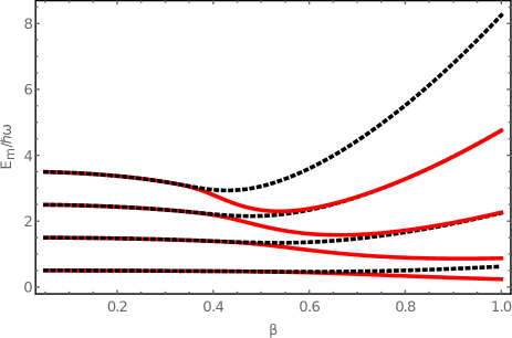
Figure 1: Plot of $E_{m}/\hbar\omega$ of polymer harmonic oscillator as a function of $\beta$ as obtained in Ref. Hossain:2010eb . The red and black (dotted) curves correspond to even ($m=2n$) and odd ($m=2n+1$) energy levels, respectively. The energy levels are degenerate up to a critical value of $\beta$.

III Construction of approximated polymer ladder operators

We aim to obtain the fluctuations in the radiation pressure on the end mirrors and that in the number of output photons in the advanced gravitational wave interferometers in the two quantization (canonical and polymer) schemes.

To compare these quantum-noises in the two quantization schemes, we need to obtain the equivalent set of approximated creation and annihilation operators in the polymer quantization scheme. Obtaining the ladder operators for the polymer harmonic oscillator is non-trivial for the following reasons: First, in standard quantization, a linear combination of position (${\hat{x}}$) and momentum (${\hat{p}}$) operators can raise or lower an energy eigenstate. In the case of polymer quantization, as can be seen from the momentum definition Eq. (8), a simple linear combination of ${\hat{x}}$ and ${\hat{P}}_{\lambda}$ does not lead to ladder operators, which can raise or lower a given polymer energy eigenstate. Second, from Fig. 1 it is evident that for $\beta\to 1$, the polymer energy eigenvalues Eq. (16) are degenerate Hossain:2010eb . Therefore, to construct the ladder operators for the case of polymer harmonic oscillator, we adopt the following procedure: we define $|0\rangle$ to be the ground state of the polymer harmonic oscillator. Let ${\hat{\alpha}}_{\lambda}$ be the annihilation operator satisfying the condition ${\hat{\alpha}}_{\lambda}|0\rangle=0$. As mentioned earlier, it is non-trivial to construct an exact annihilation operator $\hat{\alpha}_{\lambda}$ satisfying the above condition, especially in the limit of $\beta\to 1~{}(q\to 1/4)$. In the rest of this section, we construct the approximate creation and annihilation operators $(\hat{A}_{\lambda},\hat{A}_{\lambda}^{\dagger})$ for $\beta\ll 1$, satisfy the condition: ${\hat{A}}_{\lambda}|{\tilde{0}}\rangle=0$, where $|{\tilde{0}}\rangle$ is the approximate ground state of the Polymer harmonic oscillator valid in the limit $\beta\ll 1$. For small values of $\beta$, the polymer energy eigenfunctions (Eqs. (14) and (15)) can be expanded as (see Appendix. A)

$$\Psi_{2n}(p)=\left(\frac{1}{\pi\hbar m\omega}\right)^{1/4}\frac{e^{-\alpha^{2}/2}}{2^{n/2}\sqrt{n!}}\biggl{\{}{\rm H}_{n}(\alpha) - \frac{\beta^{2}}{4}\biggl{[}\frac{1}{32}H_{n+4}(\alpha)+\frac{1}{4}H_{n+2}(\alpha)+\frac{2n+1}{2}H_{n}(\alpha)$$ (17)

$$+ n(n-1)H_{n-2}(\alpha)-12~{}nC_{4}H_{n-4}(\alpha)\biggr{]}+O(\beta^{4})\biggr{\}},$$

$$\Psi_{2n+1}(p)=\left(\frac{1}{\pi\hbar m\omega}\right)^{1/4}\frac{e^{-\alpha^{2}/2}}{2^{n/2}\sqrt{n!}}\biggl{\{}{\rm H}_{n}(\alpha) - \frac{\beta^{2}}{4}\biggl{[}\frac{1}{32}H_{n+4}(\alpha)-\frac{1}{4}H_{n+2}(\alpha)-\left(\frac{2n+1}{2}-\alpha^{2}\right)H_{n}(\alpha)$$ (18)

$$- n(n-1)H_{n-2}(\alpha)-12~{}nC_{4}H_{n-4}(\alpha)\biggr{]}+O(\beta^{4})\biggr{\}},$$

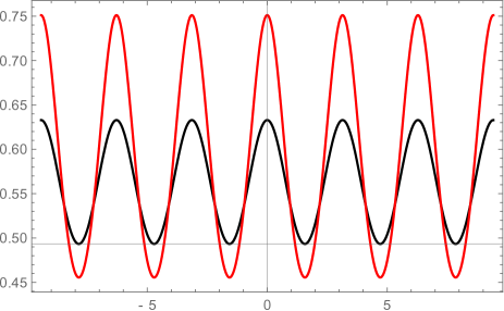
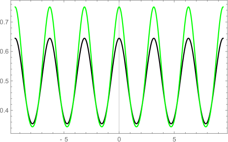
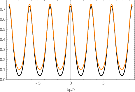
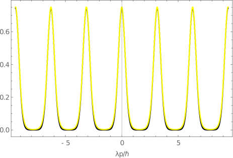
Figure 2: The plot of the scaled Polymer quantized Harmonic oscillator eigenfunctions versus dimensionless momentum ${\tilde{p}}=\lambda p/\hbar$. The black curve in all the four plots above correspond to the exact Polymer eigenfunction $(\hbar m\omega)^{1/4}\,\Psi_{n=0}(\tilde{p})$ as in Eq. (14). The Red, Green, Orange and Yellow curves correspond to the approximated Polymer eigenfunction $(\hbar m\omega)^{1/4}~{}{\widetilde{\Psi}}_{n=0}({\tilde{p}})$ for $\beta=1$ (red), $0.8$ (Green), $0.5$ (Orange), and $0.3$ (Yellow), respectively.

where $\alpha={\rm sin}(\lambda p/\hbar)/\beta$, and $H_{n}$ are the Hermite polynomials. In the leading order in $\beta$, we can approximate the polymer harmonic oscillator energy eigenfunctions (Eqs. (14) and (15)) as

$$\Psi_{2n}(p)\approx\widetilde{\Psi}_{2n}(p)=\frac{1}{\left(\pi\hbar m\omega\right)^{1/4}}\frac{e^{-\alpha^{2}/2}{\rm H}_{n}(\alpha)}{2^{n/2}\sqrt{n!}}\,.$$ (19)

Since, as mentioned earlier, $\Psi_{2n}(p)$ and $\Psi_{2n+1}(p)$ are degenerate for $\beta\ll 1$, considering only the even (or odd) eigenfunctions is adequate. Figs. 2 and 3 contain the plots of the exact and approximate polymer harmonic oscillator eigenfunctions. As can be seen from the figures, the approximate eigenfunctions is an excellent approximation of the exact eigenfunctions for small values of $\beta$, i.e., for $\beta\ll 1$. Using the approximate polymer harmonic oscillator eigenfunctions, we can now construct the approximate annihilation operator (${\hat{A}}_{\lambda}$) in the momentum basis.

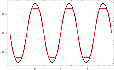
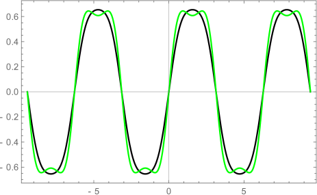
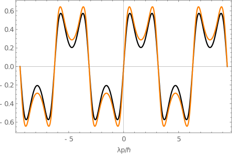
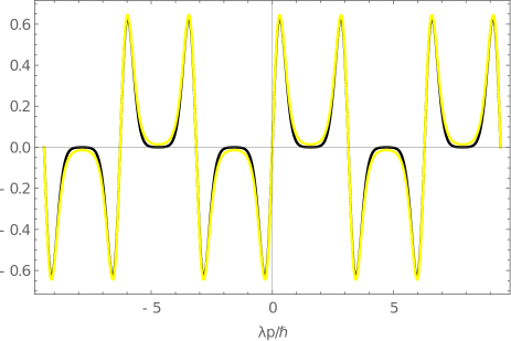
Figure 3: The plot of the scaled Polymer quantized Harmonic oscillator eigenfunctions versus dimensionless momentum ${\tilde{p}}=\lambda p/\hbar$. The black curve in all the four plots above correspond to the exact Polymer eigenfunction $(\hbar m\omega)^{1/4}\,\Psi_{n=2}(\tilde{p})$ as in Eq. (14). The Red, Green, Orange and Yellow curves correspond to the approximated Polymer eigenfunction $(\hbar m\omega)^{1/4}~{}{\widetilde{\Psi}}_{n=2}({\tilde{p}})$ for $\beta=1$ (red), $0.8$ (Green), $0.5$ (Orange), and $0.3$ (Yellow), respectively.

Using the properties of Hermite polynomials, we can rewrite the approximate eigenfunctions (Eq. 19) as:

$$\widetilde{\Psi}_{n}(p)=\frac{1}{\left(\pi\hbar m\omega\right)^{1/4}}\frac{1}{\sqrt{n!}}\left[\frac{1}{\sqrt{2}}\left(\alpha-\frac{{\rm d}}{{\rm d}\alpha}\right)\right]^{n}e^{-\alpha^{2}/2}.$$ (20)

As in canonical quantization, we can then write the approximate creation operator in the polymer quantization as:

$${\hat{A}^{\dagger}}_{\lambda}=\frac{1}{\sqrt{2}}\left(\alpha-\frac{{\rm d}}{{\rm d}\alpha}\right).$$ (21)

Thus, the approximate ladder operators corresponding to the polymer quantized harmonic oscillator energy eigenstates are:

$${\hat{A}}_{\lambda} = \frac{1}{(2\hbar m\omega)^{1/2}}\left({\hat{P}}_{\lambda}-i\frac{m\omega{\hat{x}}}{{\rm cos}(\lambda p/\hbar)}\right)\,,$$ (22)

$${\hat{A}^{\dagger}}_{\lambda} = \frac{1}{(2\hbar m\omega)^{1/2}}\left({\hat{P}}_{\lambda}+i\frac{m\omega{\hat{x}}}{{\rm cos}(\lambda p/\hbar)}\right),$$ (23)

It is easy to verify that the approximate ladder operators, corresponding to the approximate ground state of polymer harmonic oscillator (Eq. 19), satisfy the commutation relation $[{\hat{A}}_{\lambda},{\hat{A}^{\dagger}}_{\lambda}]=1$ and ${\hat{A}}_{\lambda}|{\tilde{0}}\rangle=0$. Expanding the energy eigenvalues (Eq. 16) for small values of $\beta$ leads to:

$$\frac{E_{2n}}{\hbar\omega}\approx\left(n+\frac{1}{2}\right)-\frac{\beta^{2}}{16}\left[(2n+1)^{2}+1\right]+O(\beta^{4})\,.$$ (24)

Retaining only the leading order term allows us to interpret that the $n^{\rm th}$ energy level $|{\widetilde{n}}\rangle$ contains $n$ particles, i.e., ${\hat{A}}^{\dagger}_{\lambda}{\hat{A}}_{\lambda}|{\widetilde{n}}\rangle=n|{\widetilde{n}}\rangle$. In the rest of this work, we will use the approximate ladder operators and energy values to study the implications of polymer quantization on various noises in advanced LIGO configuration.

IV Quantum-mechanical noises in advanced LIGO: Canonical Quantization

In this section, we briefly review Caves’ analysis for the advanced LIGO configuration Caves:1981 . As it is well known a gravitational wave detector is a two-arm, multi-reflecting, laser powered Michelson–Morley interferometer Caves:1981 . The interferometer measures the spatial strain produced by gravitational waves as a variation in lengths of its mutually perpendicular arms, with end mirrors attached to it. The accurate measurement of this spatial strain is limited by two main sources of quantum-mechanical noise — fluctuations in the radiation pressure on the end mirrors (radiation-pressure noise) and fluctuations in the number of output photons (photon-count noise).

Radiation pressure noise is due to the transfer of momentum, possessed by the optical field in the interferometer arms, to the end mirrors. On the other hand, the photon-counting error is due to the uncertainty produced by the photo-detectors capturing the photons leaving the interferometer arms. As mentioned in the introduction, at low-frequency, the sensitivity of these detectors is affected by seismic and radiation-pressure noise. Thus, the Einstein telescope will be sensitive to the radiation pressure. Thus, the advanced gravitational wave detectors provide a unique opportunity to distinguish between polymer quantization and canonical quantization using the radiation pressure noise curves.

IV.1 Radiation-pressure noise

As mentioned above, the radiation-pressure noise is due to the transfer of radiation field’s momentum to the end mirrors. Therefore, radiation-pressure noise is calculated by estimating the momentum carried by the radiation field in the arms of the interferometer. To carry out this, one requires four modes of the electromagnetic radiation field. Two modes, referred to as $E_{1}^{+}$ and $E_{2}^{+}$, are the in-modes, and the remaining two modes ($E_{1}^{-}$ and $E_{2}^{-}$) are out-modes . Among the in-modes, $E_{1}^{+}$ mode corresponds to the radiation field of frequency $\omega$ from the input laser port, and the $E_{1}^{-}$ mode describes radiation field from the “unused” port.

After the in-modes are scattered by the beam splitter, the “in” and “out” modes are related by Caves:1981 :

$$E^{-}_{1}=\frac{e^{-i\Delta}}{\sqrt{2}}\left(E^{+}_{1}+e^{-i\mu}E^{+}_{2}\right),$$ (25)

$$E^{-}_{2}=\frac{e^{-i\Delta}}{\sqrt{2}}\left(E^{+}_{2}-e^{i\mu}E^{+}_{1}\right),$$ (26)

where $\Delta$ and $\mu$ are the overall phase shift and relative phase shift, respectively. They depend on the intrinsic properties of the beam splitter.

The creation and annihilation operators corresponding to the input and the output modes of the interferometer are related by

$$\hat{b}_{1}=\frac{e^{i\Delta}}{\sqrt{2}}\left(\hat{a}_{1}+e^{i\mu}\hat{a}_{2}\right);$$ (27)

$$\hat{b}_{2}=\frac{e^{i\Delta}}{\sqrt{2}}\left(\hat{a}_{2}-e^{-i\mu}\hat{a}_{1}\right),$$ (28)

where $\hat{a}_{1}$, $\hat{a}_{2}$ are the annihilation operators corresponding to the input ports $(1^{+})$ and $(2^{+})$, and $\hat{b}_{1}$, $\hat{b}_{2}$ denote the annihilation operators corresponding to the output ports $(1^{-})$ and $(2^{-})$ of the interferometer.

The difference between the momenta transferred to the end masses is given by Caves:1981 :

$${\hat{\cal P}} \equiv \frac{2\nu\hbar\omega}{c}\left(\hat{b}_{2}^{\dagger}\hat{b}_{2}-\hat{b}_{1}^{\dagger}\hat{b}_{1}\right)$$ (29)

$$= -\frac{2\nu\hbar\omega}{c}\left(e^{i\mu}\hat{a}_{1}^{\dagger}\hat{a}_{2}+e^{-i\mu}\hat{a}_{2}^{\dagger}\hat{a}_{1}\right).$$

where $\nu$ is the number of times the photon bounces in the interferometer before it reaches the receiver. Squeezed states are useful for the detection of the gravitational waves, as they have a reduced uncertainty in one component of the complex amplitude. The squeezed state of the electromagnetic field can be expressed as Caves:1981 :

$$|\psi\rangle=S_{2}(\xi)D_{1}(\alpha)|0\rangle\quad\xi=-re^{i\theta},$$ (30)

where $D_{1}(\alpha)\equiv e^{-|\alpha|^{2}/2}~{}e^{\alpha a^{\dagger}_{1}}$ is the displacement operator corresponding to the mode $E_{1}^{+}$, and $\alpha$ as a complex number. The squeezing operator corresponding to the mode $E_{2}^{+}$ is defined as $S_{2}(\xi)\equiv{\rm exp}\{[\xi^{*}a_{2}^{2}-\xi(a_{2}^{\dagger})^{2}]/2\}$, with $\xi=-re^{i\theta}$. Note that $r$ and $\alpha$ are the squeezing parameters, and $\theta$ is referred to as squeezing angle.

The squeezed states satisfy the following relations:

$$\langle\psi|\hat{\cal P}|\psi\rangle=0,$$

$$\langle\psi|\left(\Delta{\cal P}\right)^{2}|\psi\rangle=(2\nu\hbar\omega/c)^{2}\biggl{[}|\alpha|^{2}{\rm cosh}(2r)+{\rm sinh}^{2}r$$

$$+ \left(\alpha^{2}e^{i(\theta+2\mu)}+\alpha^{*^{2}}e^{-i(\theta+2\mu)}\right)~{}{\rm sinh}r~{}{\rm cosh}r\biggr{]}.~{}~{}~{}$$ (32)

If $\alpha$ is real, and the squeezing angle is chosen to be $\theta=-2\mu$, then

$$\langle\psi|\left(\Delta{\cal P}\right)^{2}|\psi\rangle=(2\nu\omega)^{2}(\alpha^{2}{\rm e}^{2r}+{\rm sinh}^{2}r).$$ (33)

Note that $\mu$ is characteristic of beam splitter, hence, we can always choose $\mu$ to have a particular value.

Thus, the difference in momentum transfer on the end mirrors, for a duration of time $\tau$, leads to an error in the difference in position of the two mirrors, $z=z_{2}-z_{1}$, is given by:

$$\left(\Delta z\right)_{\rm rp}=\frac{\nu\hbar\omega\tau}{mc}\left(\alpha^{2}{\rm e}^{2r}+{\rm sinh}^{2}r\right)^{1/2}.$$ (34)

where $z_{1}$ and $z_{2}$ are the positions of the end mirrors. Note that the uncertainty in the radiation pressure translates to the error in the measurement of the gravitational wave signal and it depends on the parameters of the radiation field in the arms of the interferometer and the duration of time $\tau$.

IV.2 Photon-count noise

Photon-count error is due to the fluctuations in number of photons leaving the arms of the interferometer. The “in” and “out” modes are related by

$$E^{-}_{1}=e^{-i\Phi}\left[E^{+}_{2}{\rm cos}(\phi/2)+ie^{i\mu}E^{+}_{1}{\rm sin}(\phi/2)\right],$$ (35)

$$E^{-}_{1}=e^{-i\Phi}\left[E^{+}_{1}{\rm cos}(\phi/2)+ie^{-i\mu}E^{+}_{2}{\rm sin}(\phi/2)\right],$$ (36)

where $\phi$ is the phase difference between the output light emitted by the interferometer arms, and $\Phi$ is the mean phase. They are related to the positions of the end mirrors and the parameters of the beam splitter by the following relations Caves:1981 :

$$\phi = 2b\omega z/c+\pi-2\mu,$$ (37)

$$\Phi = b\omega(z_{1}+z_{2})/c+\Phi_{0},$$ (38)

where $\Phi_{0}$ is a constant.

The annihilation operators of the out-modes $({\hat{c}}_{1},{\hat{c}}_{2})$, are related to the annihilation operators of the in-modes (${\hat{a}}_{1}$, ${\hat{a}}_{2}$) by the following relations Caves:1981 :

$${\hat{c}}_{1} = e^{i\Phi}\left[-i{\rm e}^{-i\mu}{\hat{a}}_{1}{\rm sin}(\phi/2)+{\hat{a}}_{2}{\rm cos}(\phi/2)\right],$$ (39)

$${\hat{c}}_{2} = e^{i\Phi}\left[{\hat{a}}_{1}{\rm cos}(\phi/2)-i{\rm e}^{i\mu}{\hat{a}}_{2}{\rm sin}(\phi/2)\right].$$ (40)

For the squeezed state $|\psi\rangle$ defined in Eq. (30), the expectation value of the difference in number of photons emitted by the interference arms, and its variance are

$$n_{\rm out} \equiv \langle\psi|(\hat{c}_{2}^{\dagger}\hat{c}_{2}-\hat{c}_{1}^{\dagger}\hat{c}_{1})|\psi\rangle$$ (41)

$$= {\rm cos}\phi\left[|\alpha|^{2}-{\rm sinh}^{2}r\right]~{}~{}~{}~{}~{}~{}~{}$$

$$(\Delta n_{\rm out})^{2} = {\rm cos}^{2}\phi(|\alpha|^{2}+2{\rm sinh}^{2}r~{}{\rm cosh}^{2}r)+{\rm sin}^{2}\phi$$ (42)

$$\times \biggl{[}{-\rm sinh}r~{}{\rm cosh}r\left(\alpha^{2}e^{i(\theta+2\mu)}+\alpha^{*^{2}}e^{-i(\theta+2\mu)}\right)$$

$$+ |\alpha|^{2}{\rm cosh}(2r)+{\rm sinh}^{2}r\biggr{]}$$

Like in the previous case, choosing the $\alpha$ to be real and the squeezing angle $\theta$ to be $-2\mu$, we have

$$(\Delta n_{\rm out})^{2} = {\rm cos}^{2}\phi(\alpha^{2}+2{\rm sinh}^{2}r~{}{\rm cosh}^{2}r)$$ (43)

$$+ {\rm sin}^{2}\phi(\alpha^{2}~{}e^{-2r}+{\rm sinh}^{2}r)$$

Thus, the difference in the output photon number changes in $z$, leading to an error in the displacement of the position of the end mirrors $[(\Delta z)_{\rm pc}]$ due to the photon-count noise is given by:

$$(\Delta z)_{\rm pc}=\frac{c}{2b\omega}(\alpha^{2}-{\rm sinh}^{2}r)^{-1}$$

$$\times \biggl{[}{\rm cot}^{2}\phi~{}(\alpha^{2}+2{\rm cosh}^{2}r~{}{\rm sinh}^{2}r)+\alpha^{2}e^{-2r}+{\rm sinh}^{2}r\biggr{]}^{1/2}$$

From the above, one can extract the Caves’ limit, i.e., ${\rm cos}\,\phi=0$, and taking $|\alpha|\gg|{\rm sinh}r|$, to obtain

$$(\Delta z)_{\rm pc}\approx(c/2b\omega)\alpha^{-1}e^{-r}~{},$$ (45)

although we emphasize that we will use the exact expression (IV.2) to compare with its polymer counterpart in the following section.

In the next section, we obtain the error in the displacement of the end mirrors due to the radiation-pressure and photon-count for the polymer quantization for the advanced LIGO configuration.

V Quantum-mechanical noises in advanced LIGO: Polymer Quantization

To obtain the effects of polymer quantization on fluctuations in the radiation pressure on the end mirrors (radiation-pressure noise), and fluctuations in the number of output photons (photon-count noise), we need to polymer quantize the electromagnetic field in the interferometer arms.

In the following subsection, we perform polymer quantization of the electromagnetic field, for small values of $\beta$, and use the approximate polymer creation and annihilation operators to obtain the quantum-mechanical noises in the advanced LIGO configuration.

V.1 Polymer quantization of electromagnetic field

Assume that the electromagnetic field is confined in a cavity of volume $V$, with periodic boundary conditions. For simplicity, we assume that the cavity is a cube of length $L$. For small values of $\beta$, one can approximately decompose the electromagnetic field in the Fourier domain, the Hamiltonian corresponding to a mode ${\bf k}$ can be written as Milonni:1994xx

$$H_{\bf k}=\frac{1}{2}\int{\rm d}V\left(\epsilon_{0}E_{\bf k}^{2}+\mu_{0}^{-1}B_{\bf k}^{2}\right).$$ (46)

Decomposing the vector potential ${\bf A}$ into plane waves in the Coulomb gauge, electric and magnetic fields are given by Milonni:1994xx :

$${\bf E} = \frac{1}{\sqrt{\epsilon_{0}V}}\sum_{\bf k}{\cal E}_{\small{\bf k}}\biggl{[}\omega_{\small{\bf k}}q_{\small{\bf k}}~{}{\rm sin}(\omega_{\bf k}t-{\bf k}\cdot{\bf r})$$ (47)

$$- p_{\small{\bf k}}~{}{\rm cos}(\omega_{\small{\bf k}}t-{\bf k}\cdot{\bf r})\biggr{]},$$

$${\bf B} = \sqrt{\frac{\mu_{0}}{V}}\sum_{\bf k}({\hat{\bf k}}\times{\cal E}_{\small{\bf k}})\biggl{[}\omega_{\small{\bf k}}q_{\small{\bf k}}~{}{\rm sin}(\omega_{\bf k}t-{\bf k}\cdot{\bf r})$$ (48)

$$- p_{\small{\bf k}}~{}{\rm cos}(\omega_{\small{\bf k}}t-{\bf k}\cdot{\bf r})\biggr{]},$$

where

$$q_{\small{\bf k}}=\sqrt{\frac{\hbar}{2\omega_{\small{\bf k}}}}(a^{*}_{\small{\bf k}}+a_{\small{\bf k}});~{}p_{\small{\bf k}}=\sqrt{\frac{\hbar\omega_{\small{\bf k}}}{2}}(a^{*}_{\small{\bf k}}-a_{\small{\bf k}}).$$ (49)

Substituting Eqs. (47) and (48) in the Hamiltonian, i.e., in Eq. (46), we get:

$$H_{\bf k}=\frac{1}{2}\left(p_{\small{\bf k}}^{2}+\omega_{\small{\bf k}}^{2}q_{\small{\bf k}}^{2}\right).$$ (50)

To proceed with the polymer quantization of electromagnetic fields, for small values of $\beta$, we need to polymer quantize the individual harmonic oscillators corresponding to different frequency modes ($\omega_{\bf k}$), i. e.,

$$H_{\bf k(\lambda)}=\frac{1}{2}\left[\left(P_{\small{\bf k}(\lambda)}\right)^{2}+\omega_{\small{\bf k}}^{2}q_{\small{\bf k}}^{2}\right],$$ (51)

where

$$P_{\small{\bf k}(\lambda)}=\frac{{\hat{U}}_{\small{\bf k}(\lambda)}-{\hat{U}}^{\dagger}_{\small{\bf k}(\lambda)}}{2i\lambda},$$ (52)

with ${\hat{U}}_{\small{\bf k}(\lambda)}$ as the translation operator associated with the harmonic oscillator corresponding to the mode ${\bf k}$ as defined in Eq. (7).

As seen in the previous section, to obtain the expressions for radiation-pressure and photon-count noises, we need to define the creation and annihilation operators in the Fock space. For the case of polymer harmonic oscillator, as shown in Sec. (III), it is possible to define these operators in the limit $\beta\ll 1$. In this limit we can define an approximate polymer harmonic oscillator state $|{\widetilde{\Psi}}\rangle$ in the Fock basis (Eq. (19)). The approximate state allows us to define the displacement and squeezing operators in the polymer quantization for the approximate ground state $|\tilde{0}\rangle$. Though the approximate creation/annihilation operators satisfy $[{\hat{A}}_{\lambda},{\hat{A}}^{\dagger}_{\lambda}]=1$, the effect of polymer quantization effectively comes from the approximated polymer quantum state $|{\widetilde{\Psi}}\rangle$. In the rest of this section, we obtain the fluctuations in the radiation pressure on the mirrors (radiation-pressure noise) and fluctuations in the number of output photons (photon-count noise) for the polymer quantized electromagnetic field in the interferometer arms.

V.2 Radiation-pressure noise

Let ${\hat{A}}_{\lambda(1)}$, ${\hat{A}}_{\lambda(2)}$ be the polymer annihilation operators corresponding to the input ports ($1^{+}$) and ($2^{+}$), and ${\hat{B}}_{\lambda(1)}$, ${\hat{B}}_{\lambda(2)}$ be the polymer annihilation operators corresponding to the output ports ($1^{-}$) and ($2^{-}$) of the interferometer.

In the polymer quantization, the difference between momenta transferred to the end mirrors is given by:

$$\hat{\widetilde{\cal P}} \equiv (2\nu\hbar\omega/c)\left({\hat{B}}_{\lambda(2)}^{\dagger}{\hat{B}}_{\lambda(2)}-{\hat{B}}_{\lambda(2)}^{\dagger}{\hat{B}}_{\lambda(2)}\right),$$ (53)

$$= -(2\nu\hbar\omega/c)\left(e^{i\mu}{\hat{A}}_{\lambda(1)}^{\dagger}{\hat{A}}_{\lambda(2)}+e^{-i\mu}{\hat{A}}_{\lambda(2)}^{\dagger}{\hat{A}}_{\lambda(1)}\right).~{}~{}~{}~{}~{}$$ (54)

Here again, we consider squeezing the approximate ground state as shown below,

$$|{\widetilde{\psi}}\rangle={\widetilde{S}}_{2}(\xi){\widetilde{D}}_{1}(\alpha)|\tilde{0}\rangle,$$ (55)

where the polymer modified squeezing and displacement operators are defined as

$${\widetilde{S}}(\xi) \equiv {\rm exp}\left\{[\xi^{*}({\hat{A}}_{\lambda})^{2}-\xi~{}({{\hat{A}}^{\dagger}}_{\lambda})^{2}]/2\right\},$$ (56)

$${\widetilde{D}}(\alpha) \equiv {\rm exp}\left(\alpha{{\hat{A}}^{\dagger}}_{\lambda}-\alpha^{*}{\hat{A}}_{\lambda}\right);\,~{}~{}\xi=-re^{i\theta}\,.$$ (57)

For the polymer modified squeezed state, we get

$$\langle{\widetilde{\psi}}|{\widetilde{\cal P}}|{\widetilde{\psi}}\rangle=0,$$

$$\langle{\widetilde{\psi}}|\left(\Delta{{\widetilde{\cal P}}}\right)^{2}|{\widetilde{\psi}}\rangle=(2\,n\,\hbar\omega/c)^{2}\biggl{[}|\alpha|^{2}{\rm cosh}(2r)+{\rm sinh}^{2}r$$

$$~{}~{}~{}~{}+\left(\alpha^{2}e^{i(\theta+2\mu)}+\alpha^{*^{2}}e^{-i(\theta+2\mu)}\right){\rm sinh}r~{}{\rm cosh}r\biggr{]}$$

$$~{}~{}~{}~{}\times\frac{\sqrt{\pi}}{\beta}e^{-1/2\beta^{2}}I_{0}(1/2\beta^{2}),$$ (59)

where, $I_{0}$ is the modified Bessel function of the first kind,

$$\beta=\sqrt{\frac{\hbar\omega}{M_{*}c^{2}}}\,,$$ (60)

and $M_{*}$ be the energy scale (inverse of polymer length scale $\lambda$) associated with the polymer quantization.

This is an important result, and we would like to stress the following points: First, like in canonical quantization, Eq. (V.2) implies that the average number of polymer particles are same in both the interferometer arms. This is not the case for other quantum gravity inspired models such as GUP.

In the case of GUP, it was shown that the expectation value of the difference in momentum transfer is non-zero Bosso:2018 , however the expectation of difference in momentum transfer vanishes for the case of polymer quantization. Second, fluctuations in the momentum transfer, Eq. (59), is different from that of the canonical quantization. As in the case of canonical quantization, choosing the squeezing angle to be $\theta=-2\mu$, we get

$$\langle{\widetilde{\psi}}|\left(\Delta{{\widetilde{\cal P}}}\right)^{2}|{\widetilde{\psi}}\rangle = \left(\frac{2\,n\,\hbar\omega}{c}\right)^{2}(\alpha^{2}{\rm e}^{2r}+{\rm sinh}^{2}r)$$ (61)

$$\times \frac{\sqrt{\pi}}{\beta}e^{-1/2\beta^{2}}I_{0}(1/2\beta^{2}),$$

Third, the difference in momentum transfer on the end mirrors, for a duration of time $\tau$, leads to the following error $[(\Delta{\widetilde{z}})_{\rm rp}]$

$$\Delta{\widetilde{z}}_{\rm rp}=\frac{n\hbar\omega\tau}{mc}\left(\alpha^{2}{\rm e}^{2r}+{\rm sinh}^{2}r\right)^{1/2}\left[\frac{\sqrt{\pi}}{\beta}\frac{I_{0}(1/2\beta^{2})}{e^{1/2\beta^{2}}}\right]^{1/2}$$ (62)

Let $\Delta_{\rm rp}$ be the ratio of the radiation-pressure error in the polymer quantization [$\Delta{\widetilde{z}}_{\rm rp}$] and the same in the canonical quantization [$\Delta{z}_{\rm rp}$], i. e.,

$$\Delta_{\rm rp}(\beta)=\left[\frac{\sqrt{\pi}}{\beta}e^{-1/2\beta^{2}}I_{0}(1/2\beta^{2})\right]^{1/2},$$ (63)

Fig. (4) contains plot of $\Delta_{\rm rp}(\beta)$ as a function of $\beta$. It is clear that in the limit $\beta\to 0$, the ratio is unity. However, even if $\beta\simeq 0.1$, the difference between the two quantization schemes is order of $10^{-3}$.

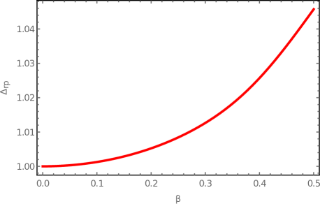
Figure 4: The plot of $\Delta_{\rm rp}$ as a function of $\beta$.

V.3 Photon-count noise

Let ${\hat{C}}_{\lambda(1)}$ and ${\hat{C}}_{\lambda(2)}$ be the annihilation operators corresponding to the out-modes. The annihilation operators corresponding to the “in” modes (${\hat{A}}_{\lambda(1)}$, ${\hat{A}}_{\lambda(2)}$) are related to that of “out” modes by the following relations:

$${\widehat{C}}_{\lambda(1)} = e^{i\Phi}\left[{\widehat{A}}_{\lambda(2)}{\rm cos}(\phi/2)-i{\rm e}^{-i\mu}{\widehat{A}}_{\lambda(1)}{\rm sin}(\phi/2)\right],~{}~{}~{}~{}~{}$$ (64)

$${\widehat{C}}_{\lambda(2)} = e^{i\Phi}\left[{\widehat{A}}_{\lambda(1)}{\rm cos}(\phi/2)-i{\rm e}^{i\mu}{\widehat{A}}_{\lambda(2)}{\rm sin}(\phi/2)\right].$$ (65)

For the squeezed state $|{\widetilde{\psi}}\rangle$ defined in Eq. (55), the expectation value of the difference in the number of polymer photons emitted by the interferometer arms, and its variance are

$${\widetilde{n}}_{\rm out} \equiv \langle{\widetilde{\psi}}|({{\widehat{C}}_{\lambda(2)}}^{\dagger}{\widehat{C}}_{\lambda(2)}-{{\widehat{C}}_{\lambda(1)}}^{\dagger}{\widehat{C}}_{\lambda(1)})|{\widetilde{\psi}}\rangle$$ (66)

$$= {\rm cos}\phi\left(|\alpha|^{2}-{\rm sinh}^{2}r\right)$$

$$\times \frac{\sqrt{\pi}}{\beta}e^{-1/2\beta^{2}}I_{0}(1/2\beta^{2})$$

$$(\Delta{\widetilde{n}}_{\rm out})^{2} = \biggl{\{}{\rm cos}^{2}\phi(|\alpha|^{2}+2{\rm sinh}^{2}r~{}{\rm cosh}^{2}r)+{\rm sin}^{2}\phi$$ (67)

$$\times \biggl{[}{-\rm sinh}r~{}{\rm cosh}r\left(\alpha^{2}e^{i(\theta+2\mu)}+\alpha^{*^{2}}e^{-i(\theta+2\mu)}\right)$$

$$+ |\alpha|^{2}{\rm cosh}(2r)+{\rm sinh}^{2}r\biggr{]}+{\rm cos}^{2}\phi~{}{\rm sinh}^{4}r$$

$$\times \left(1-\frac{\sqrt{\pi}}{\beta}e^{-1/2\beta^{2}}I_{0}(1/2\beta^{2})\right)\biggr{\}}$$

$$\times \frac{\sqrt{\pi}}{\beta}e^{-1/2\beta^{2}}I_{0}(1/2\beta^{2})$$

As in the case of canonical quantization, taking $\alpha$ to be real, and $\theta=-2\mu$ in Eq. (67), we get:

$$(\Delta{\widetilde{n}}_{\rm out})^{2} = \biggl{[}{\rm cos}^{2}\phi(\alpha^{2}+2{\rm sinh}^{2}r{\rm cosh}^{2}r)$$ (68)

$$+ {\rm sin}^{2}\phi(\alpha^{2}e^{-2r}+{\rm sinh}^{2}r)+{\rm cos}^{2}\phi~{}{\rm sinh}^{4}r$$

$$\times \left(1-\frac{\sqrt{\pi}}{\beta}e^{-1/2\beta^{2}}I_{0}(1/2\beta^{2})\right)\biggr{]}$$

$$\times \frac{\sqrt{\pi}}{\beta}e^{-1/2\beta^{2}}I_{0}(1/2\beta^{2})$$

The difference in the output photon number changes with respect to $z$, and hence leads to error in the displacement of the position of the end mirrors $[(\Delta{\widetilde{z}})_{\rm pc}]$. Therefore, the photon-count noise is given by:

$$\Delta{\widetilde{z}}_{\rm pc} = \frac{c}{2b\omega}(\alpha^{2}-{\rm sinh}^{2}r)^{-1}$$ (69)

$$\times \biggl{[}{\rm cos}^{2}\phi(\alpha^{2}+2{\rm sinh}^{2}r{\rm cosh}^{2}r)$$

$$+ {\rm sin}^{2}\phi(\alpha^{2}e^{-2r}+{\rm sinh}^{2}r)+{\rm cos}^{2}\phi~{}{\rm sinh}^{4}r$$

$$\times \left(1-\frac{\sqrt{\pi}}{\beta}e^{-1/2\beta^{2}}I_{0}(1/2\beta^{2})\right)\biggr{]}^{1/2}$$

$$\times \left[\frac{\sqrt{\pi}}{\beta}e^{-1/2\beta^{2}}I_{0}(1/2\beta^{2})\right]^{1/2}$$

Again, similar to canonical quantization, setting ${\rm cos}\,\phi=0$, we get

$$\Delta{\widetilde{z}}_{\rm pc} = \frac{c}{2b\omega}(\alpha^{2}-{\rm sinh}^{2}r)^{-1}$$ (70)

$$\times \biggl{(}{\rm sin}^{2}\phi(\alpha^{2}e^{-2r}+{\rm sinh}^{2}r)\biggr{)}^{1/2}$$

$$\times \left[\frac{\sqrt{\pi}}{\beta}e^{-1/2\beta^{2}}I_{0}(1/2\beta^{2})\right]^{1/2}.$$

This is an important result and we would like to stress the following points: First, the fluctuations in the number of output photons in the two quantization schemes (canonical and polymer) are different. Second, let us define $\Delta_{\rm pc}$ as the ratio of photon-count error in the polymer quantization [$\Delta{\widetilde{z}}_{\rm pc}$] and the same in the canonical quantization [$\Delta{z}_{\rm pc}$]. The ratio $\Delta_{\rm pc}$ is plotted as shown below:

$$\Delta_{\rm pc}(\beta)=\left[\frac{\sqrt{\pi}}{\beta}e^{-1/2\beta^{2}}I_{0}(1/2\beta^{2})\right]^{1/2},$$ (71)

Thus, $\Delta_{\rm pc}(\beta)$ is identical to $\Delta_{\rm rp}(\beta)$, i.e. the functional dependence of the quantum noises on $\beta$ is identical. Third, the effects due to Polymer quantization is different from that of the GUP Bosso:2018 . As mentioned earlier, the expectation value of the difference in momentum transfer is non-zero for the case of GUP Bosso:2018 , however, the expectation of difference in momentum transfer vanishes for the case of polymer quantization. On the other hand, the GUP corrections to the radiation-pressure and photon-count noises are not the same Bosso:2018 . It is also interesting to note that the effects of polymer quantization on the radiation-pressure and photon-count noises are strikingly different from that of GUP.

VI Conclusions and Discussions

We have investigated, in detail, the experimental signatures of the polymer quantization on the quantum-mechanical noises in the advanced gravitational wave detectors. This is feasible only if the polymer quantized electromagnetic modes can be expressed in the Fock space. We explicitly showed that it is possible to obtain a set of approximate annihilation and creation operators in the polymer quantized harmonic oscillator in the limit $\beta\ll 1$.

We used the advanced LIGO configuration to obtain the fluctuations in the radiation pressure on the mirrors and the fluctuations in the number of output photons in the polymer quantization scheme. The photon-count error ratio ($\Delta_{\rm pc}(\beta)$) is shown to be identical to the radiation-pressure error ratio ($\Delta_{\rm rp}(\beta)$), where $\beta$ depends on the Polymer scale $M_{*}$ and the frequency of the electromagnetic field $\omega$. Note that, for the case of GUP, it was shown that the error ratios ($\Delta_{\rm rp}$ and $\Delta_{\rm pc}$) are not identical Bosso:2018 .

If the polymer energy scale $M_{*}$ is assumed to be of the order of Planck scale, then, for more realistic value of $\omega$, i.e., $2.82\times 10^{14}$ Hz LIGO-a ; LIGO-b , the parameter $\beta$ is of the order of $10^{-13}$. For small values of $\beta$ the error ratios, both $\Delta_{\rm rp}$ and $\Delta_{\rm pc}$ (denoted as $\Delta$), can be expanded as

$$\Delta=1+\frac{\beta^{2}}{8}+O(\beta^{4})\,.$$ (72)

Hence, for realistic values of the frequency of the optical field, the next to leading order contribution is roughly $10^{26}$ times smaller than the zeroth order contribution.

As mentioned before, we did not take into consideration the effects of modified dispersion relation introduced by polymer quantization. Motivated by the modified dispersion relation due to polymer quantization of scalar field in Ref. Hossain:2010eb , it possible that the polymer quantization of Maxwell field can lead to a modified dispersion of the form

$$\omega^{2}=|{\bf k}|^{2}\left[1+\delta~{}\beta^{2}+O(\beta^{4})\right],$$ (73)

in the limit $\beta\ll 1$, where $\delta$ is a constant. If $\delta$ is positive, the dispersion relation is superluminal, and if it is negative, then the relation is subluminal. For the above modification, repeating the analysis in Sec. (V), the error ratios $\Delta_{rp}$ and $\Delta_{pc}$ are given by:

$$\Delta_{rp} = 1+\left(\frac{1}{8}+\frac{\delta}{2}\right)\beta^{2}+O(\beta^{4})$$ (74)

$$\Delta_{pc} = 1+\left(\frac{1}{8}-\frac{\delta}{2}\right)\beta^{2}+O(\beta^{4})$$ (75)

Note that even if $|\delta|=1/4$ either one of $\Delta_{rp}$ and $\Delta_{pc}$ will be non-zero. Therefore, it is evident that the corrections due to modified dispersion relation is of the same order that we have considered in this work.

In the case of GUP, the expectation value of the difference in momentum transfer is non-zero ($\langle{\widetilde{\cal P}}\rangle\neq 0$) and the quantum noises in the interferometer is lower than the canonical quantization Bosso:2018 . However, in the case of Polymer quantization, the expectation value of the difference in momentum transfer is zero, and the quantum noises in the interferometer are higher than the canonical quantization. Since, $\langle(\Delta{\widetilde{\cal P}})^{2}\rangle=\langle{\widetilde{\cal P}}^{2}\rangle-\langle{\widetilde{\cal P}}\rangle^{2}$, it is clear that the models that lead to zero (or non-zero) expectation value of the difference in momentum transfer will lead to higher (or lower) quantum noises in the interferometer than the canonical quantization. This feature provides a robust test to distinguish between the two broad categories of quantum gravity phenomenological models.

The analysis in this work is done for a fixed frequency of the electromagnetic field assuming that the mode decouple and have a linear-dispersion relation. While it is true for canonical quantization, it is unclear whether this feature holds for polymer quantization Husain.Louka ; Kajuri:2015oza ; Stargen:2017 . While the ladder operators in standard harmonic oscillator are linear combinations of momentum and position operators, the approximate ladder operators for the case of approximate energy eigenfunctions of polymer harmonic oscillator have a nontrivial combination of ${\hat{x}}$ and ${\hat{p}}$:

$${\hat{A}}_{\lambda} = \frac{1}{(2\hbar m\omega)^{1/2}}\left({\hat{P}}_{\lambda}-i\frac{m\omega{\hat{x}}}{{\rm cos}(\lambda p/\hbar)}\right)\,,$$ (76)

$${\hat{A}}^{\dagger}_{\lambda} = \frac{1}{(2\hbar m\omega)^{1/2}}\left({\hat{P}}_{\lambda}+i\frac{m\omega{\hat{x}}}{{\rm cos}(\lambda p/\hbar)}\right).$$ (77)

The next step in the analysis is to investigate the quantum mechanical noises due to polymer quantization in the gravitational wave frequency band for the ground-based and space-based detectors i.e. $10^{-5}~{}{\rm Hz}$ to $50~{}{\rm Hz}$. Such an analysis will provide us the tools for testing these results. This work is in progress.

As we were finalizing this manuscript, the article Gianluca:2019 appeared that discusses plausible quantum gravity signatures in future gravitational wave observations, such as gravitational wave luminosity distance, the time dependence of effective Planck mass, and also the instrumental strain noise of interferometers. The focus of this work is different from Ref. Gianluca:2019 , which is to analyze the difference in effects due to the quantization schemes on the interferometer noises.

Appendix A Asymptotic expansion of polymer energy eigenfunctions for large values of $q$

In this appendix, following Ref. Blanch:1960 , we explicitly show the asymptotic expansion of energy eigenfunctions of polymer harmonic oscillator , $\Psi_{2n}(p)$ and $\Psi_{2n+1}(p)$, for large values of $q$.

Following Eqs. (14) and (15), the polymer energy eigenfunctions in momentum basis are given by:

$$\Psi_{2n}(z) = \frac{\left(2\beta/\pi\right)^{1/2}}{\left(\hbar m\omega\right)^{1/4}}{\rm Ce}_{n}\left(q,z\right),$$ (78)

$$\Psi_{2n+1}(z) = \frac{\left(2\beta/\pi\right)^{1/2}}{\left(\hbar m\omega\right)^{1/4}}{\rm Se}_{n+1}\left(q,z\right),~{}~{}$$ (79)

where $q=1/(4\beta^{4})$, and ${\rm Ce}_{n}$, ${\rm Se}_{n}$ are Mathieu functions.

For large values of $q$, the Mathieu functions ${\rm Ce}_{n}(q,z)$ and ${\rm Se}_{n+1}(q,z)$ can be written as Blanch:1960 :

$${\rm Ce}_{n}(q,z) = \frac{(\pi/4)^{1/4}q^{1/8}}{\sqrt{n!}}~{}U_{0}\left[{\cal Z}_{0,n}(\gamma)+{\cal Z}_{1,n}(\gamma)\right],$$ (80)

$${\rm Se}_{n+1}(q,z) = \frac{(\pi/4)^{1/4}q^{1/8}}{\sqrt{n!}}~{}V_{0}\left[{\cal Z}_{0,n}(\gamma)-{\cal Z}_{1,n}(\gamma)\right]{\rm sin}z,$$ (81)

where

$$\gamma = 2q^{1/4}{\rm cos}z,$$ (82)

$$U_{0} = 1-\frac{(2n+1)}{16\sqrt{q}}+O(1/q),$$ (83)

$$V_{0} = 1+\frac{(2n+1)}{16\sqrt{q}}+O(1/q),$$ (84)

$${\cal Z}_{0,n}(\gamma) = D_{n}+\frac{1}{4\sqrt{q}}\left(\frac{n!}{16(n-4)!}D_{n-4}(\gamma)-\frac{1}{16}D_{n+4}(\gamma)\right)+O(1/q),$$ (85)

$${\cal Z}_{1,n}(\gamma) = -\frac{1}{4\sqrt{q}}\left(\frac{n(n-1)}{4}D_{n-2}(\gamma)+\frac{1}{4}D_{n+2}(\gamma)\right)+O(1/q),$$ (86)

$$D_{m}(\gamma) \equiv (-1)^{m}e^{\gamma^{2}/4}\frac{{\rm d}^{m}}{{\rm d}\gamma^{m}}e^{-\gamma^{2}/2}=\frac{e^{-\gamma^{2}/4}}{2^{m/2}}H_{m}(\gamma/\sqrt{2}).$$ (87)

Substituting Eqs. (82) - (87) in Eqs. (80) and (81), we obtain

$${\rm Ce}_{n}(q,z)=\frac{(\pi/4)^{1/4}q^{1/8}}{\sqrt{n!}}\frac{e^{-\gamma^{2}/4}}{2^{n/2}}\biggl{\{}{\rm H}_{n}(\gamma/\sqrt{2}) - \frac{1}{8\sqrt{q}}\biggl{[}\frac{1}{32}H_{n+4}(\gamma/\sqrt{2})+\frac{1}{4}H_{n+2}(\gamma/\sqrt{2})+\frac{2n+1}{2}H_{n}(\gamma/\sqrt{2})$$ (88)

$$+ n(n-1)H_{n-2}(\gamma/\sqrt{2})-\frac{n!}{2(n-4)!}H_{n-4}(\gamma/\sqrt{2})\biggr{]}+O(1/q)\biggr{\}},~{}~{}~{}~{}$$

$${\rm Se}_{n+1}(q,z)=\frac{(\pi/4)^{1/4}q^{1/8}}{\sqrt{n!}}\frac{e^{-\gamma^{2}/4}}{2^{n/2}}\biggl{\{}{\rm H}_{n}(\gamma/\sqrt{2}) - \frac{1}{8\sqrt{q}}\biggl{[}\frac{1}{32}H_{n+4}(\gamma/\sqrt{2})-\frac{1}{4}H_{n+2}(\gamma/\sqrt{2})-\left(\frac{2n+1}{2}-\gamma^{2}\right)H_{n}(\gamma/\sqrt{2})$$ (89)

$$- n(n-1)H_{n-2}(\gamma/\sqrt{2})-\frac{n!}{2(n-4)!}H_{n-4}(\gamma/\sqrt{2})\biggr{]}+O(1/q)\biggr{\}},$$

where $H_{n}$ is the Hermite polynomial. Making use of the variables defined in Eqs. (12) and (13), and the asymptotic expansions in Eqs. (88) and (89), we obtain

$$\Psi_{2n}(p)=\left(\frac{1}{\pi\hbar m\omega}\right)^{1/4}\frac{e^{-\alpha^{2}/2}}{2^{n/2}\sqrt{n!}}\biggl{\{}{\rm H}_{n}(\alpha) - \frac{\beta^{2}}{4}\biggl{[}\frac{1}{32}H_{n+4}(\alpha)+\frac{1}{4}H_{n+2}(\alpha)+\frac{2n+1}{2}H_{n}(\alpha)$$ (90)

$$+ n(n-1)H_{n-2}(\alpha)-12~{}nC_{4}H_{n-4}(\alpha)\biggr{]}+O(\beta^{4})\biggr{\}},$$

$$\Psi_{2n+1}(p)=\left(\frac{1}{\pi\hbar m\omega}\right)^{1/4}\frac{e^{-\alpha^{2}/2}}{2^{n/2}\sqrt{n!}}\biggl{\{}{\rm H}_{n}(\alpha) - \frac{\beta^{2}}{4}\biggl{[}\frac{1}{32}H_{n+4}(\alpha)-\frac{1}{4}H_{n+2}(\alpha)-\left(\frac{2n+1}{2}-2\alpha^{2}\right)H_{n}(\alpha)$$ (91)

$$- n(n-1)H_{n-2}(\alpha)-12~{}nC_{4}H_{n-4}(\alpha)\biggr{]}+O(\beta^{4})\biggr{\}},$$

where $\alpha={\rm sin}(\lambda p/\hbar)/\beta$. Note that in the limit $\lambda\to 0$, one can obtain the energy eigenfunctions of the canonically quantized simple harmonic oscillator.

References

- (1) G. Amelino-Camelia, Lect. Notes Phys. 669, 59 (2005) D. Mattingly, Living Rev. Rel. 8, 5 (2005).
- (2) S. Hossenfelder and L. Smolin, Phys. Canada 66, 99 (2010).
- (3) G. Amelino-Camelia, Living Rev. Rel. 16, 5 (2013).
- (4) T. Thiemann, Modern Canonical Quantum General Relativity Cambridge University Press, Cambridge, England (2007).
- (5) C. Rovelli, Quantum Gravity Cambridge University Press, Cambridge, England (2004).
- (6) A. Ashtekar, J. Lewandowski and H. Sahlmann, Class. Quant. Grav. 20, L11 (2003).
- (7) A. Ashtekar, S. Fairhurst and J. L. Willis, Class. Quant. Grav. 20, 1031 (2003).
- (8) G. M. Hossain, V. Husain and S. S. Seahra, Phys. Rev. D 80, 044018 (2009).
- (9) G. M. Hossain, V. Husain and S. S. Seahra, Phys. Rev. D 82, 124032 (2010).
- (10) A. Garcia-Chung and J. D. Vergara, Int. J. Mod. Phys. A 31, 1650166 (2016).
- (11) G. M. Hossain and G. Sardar, arXiv:1705.01431 [gr-qc].
- (12) Lean A. Takhtajan, Quantum Mechanics for Mathematicians (Graduate Studies in Mathematics. Vol. 95; American Mathematical Society, 2008).
- (13) S. L. Danilishin, F. Y. Khalili and H. Miao, Living Rev. Rel. 22, no. 1, 2 (2019).
- (14) Benjamin P Abbott et al. Class. Quant. Grav., 34, 044001 (2017).
- (15) C. M. Caves, Phys. Rev. D 23, 1693 (1981).
- (16) C. Corduneaunu, Almost Periodic Functions (Interscience, New York, 1968); E. Hewitt and K. A. Ross, Abstract Harmonic Analysis (Academic, New York, 1963), Vol. 1.
- (17) H. Halvorson, Stud. Hist. Phil. Mod. Phys. 35, 45 (2004).
- (18) M Abramowitz and I A. Stegun, Handbook of Mathematical Functions (Dover, New York, 1972).
- (19) A. Kempf, R. B. Mann, G. Mangano, Phys.Rev.D52, 1108-1118 (1995).
- (20) P. W. Milonni, The Quantum vacuum: An Introduction to quantum electrodynamics (Academic Press, Boston, 1994).
- (21) P. Bosso, S. Das and R. B. Mann, Phys. Lett. B 785, 498 (2018).
- (22) J. Abadie, et al., Nature Physics, 7, 962 (2011).
- (23) J. Aasi, et al., Class. Quant. Grav. 32, 074001 (2015).
- (24) V. Husain and J. Louko, Phys. Rev. Lett. 116, no. 6, 061301 (2016).
- (25) N. Kajuri, Class. Quant. Grav. 33, 055007 (2016).
- (26) D. Jaffino Stargen, Nirmalya Kajuri, and L. Sriramkumar, Phys. Rev. D 96, 066002 (2017).
- (27) G. Calcagni, S. Kuroyanagi, S. Marsat, M. Sakellariadou, N. Tamanini, G. Tasinato, [arXiv:1907.02489 [gr-qc]].
- (28) G. Blanch, Trans. Amer. Math. Soc. 97, 357 (1960).