Heteroclinic and Homoclinic Connections in a Kolmogorov-Like Flow

Abstract

Recent studies suggest that unstable recurrent solutions of the Navier-Stokes equation provide new insights into dynamics of turbulent flows. In this study, we compute an extensive network of dynamical connections between such solutions in a weakly turbulent quasi-two-dimensional Kolmogorov flow that lies in the inversion-symmetric subspace. In particular, we find numerous isolated heteroclinic connections between different types of solutions – equilibria, periodic, and quasi-periodic orbits – as well as continua of connections forming higher-dimensional connecting manifolds. We also compute a homoclinic connection of a periodic orbit and provide strong evidence that the associated homoclinic tangle forms the chaotic repeller that underpins transient turbulence in the symmetric subspace.

I Introduction

Turbulent fluid flows are ubiquitous; they can be found in the atmosphere and the oceans, water and oil pipelines, and even in the human aorta. Despite its great practical relevance, a tractable description of turbulent dynamics has remained elusive. However, recent numerical Kerswell (2005); Kawahara et al. (2012) and experimental Hof et al. (2004); de Lozar et al. (2012); Suri et al. (2017) studies have shown that unstable recurrent solutions of the Navier Stokes equation, which governs fluid flows, may prove pivotal in solving this longstanding problem. Often termed Exact Coherent States (ECSs), such solutions exist for the same parameters as turbulence but are more amenable to numerical analysis given their simple (e.g., steady or periodic) temporal behavior.

The state space description of turbulence best illustrates the dynamical role of ECSs Hopf (1948); Gibson et al. (2008). A turbulent flow in physical space maps to a winding trajectory in state space, with each point on it representing a flow field (see supplementary videos 1-7) . In contrast, ECSs such as steady and time-periodic flows are simpler objects (fixed points, closed loops), as shown in Fig. 1. Being unstable, each ECS is a saddle in state space; trajectories in its unstable manifold are repelled away, while those in the stable manifold converge to the ECS Duguet et al. (2008a); Viswanath and Cvitanovic (2009); Suri et al. (2017, 2018). Heteroclinic (homoclinic) trajectories – which originate in the unstable manifold of an ECS and terminate in the stable manifold of another (the same) ECS – connect different ECSs and create a chaotic saddle in state space Halcrow et al. (2009); Duguet et al. (2008a); Farano et al. (2018). Dynamics on ECSs, their stable manifolds, and on homo/heteroclinic connections are asymptotically non-chaotic. In this geometrical picture, turbulence represents a deterministic walk between neighborhoods of different ECSs, guided by the corresponding dynamical connections Kerswell and Tutty (2007); Suri et al. (2017), both homoclinic and heteroclinic.

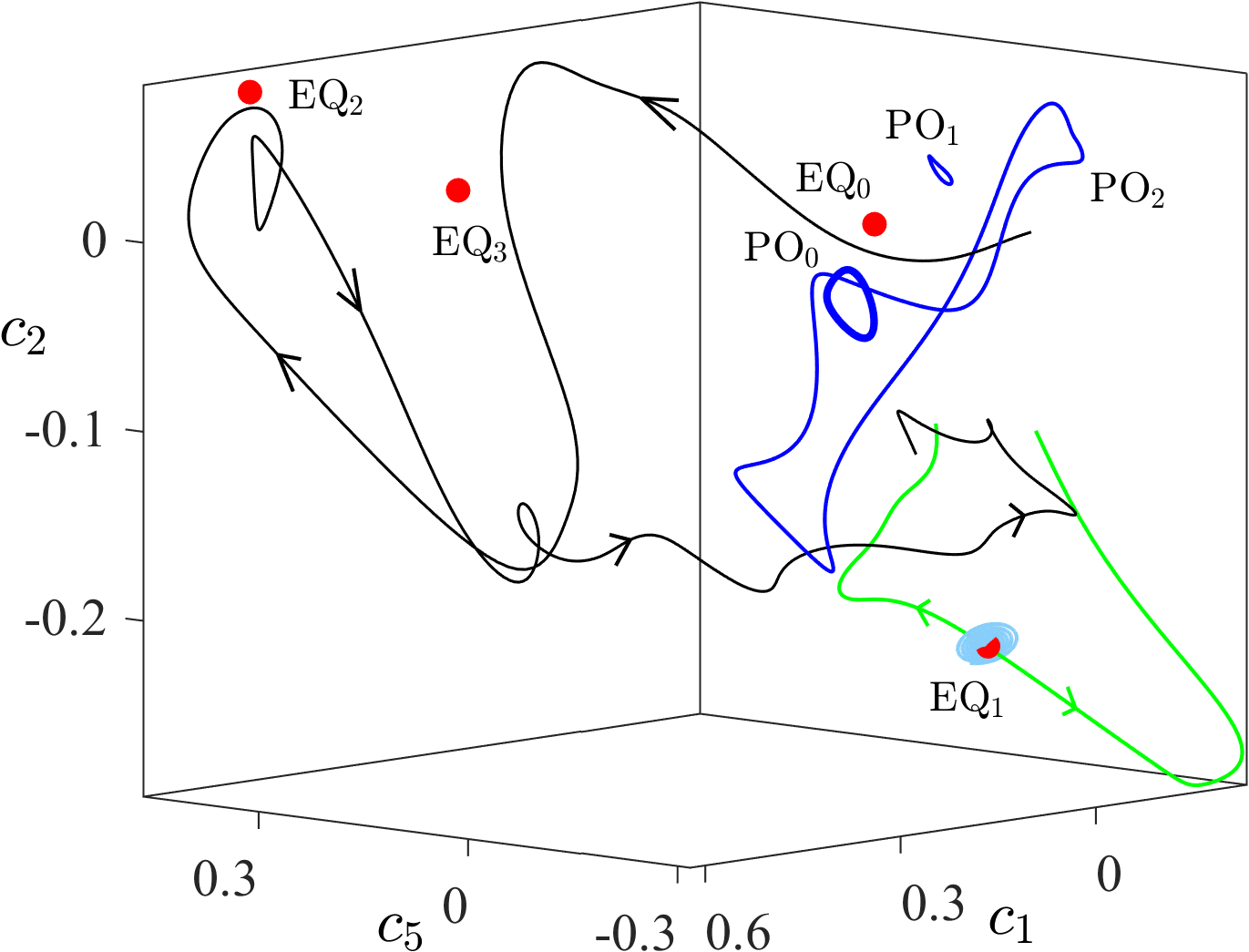
Figure 1: Low-dimensional projection of the state space generated using data from numerical simulation of a weakly turbulent Kolmogorov-like flow. Instantaneous snapshots of the flow in the physical space are associated with points in the state space. Turbulent evolution is represented by a trajectory (black curve) passing through neighborhoods of unstable equilibria (spheres) and periodic orbits (loops). Stable and unstable manifolds (green curves and light blue surface) of these solutions constrain the dynamics in their neighborhoods. The projection method is described in Appendix A.

Substantial numerical evidence has emerged for the dynamical relevance of ECSs in recent years, mostly from research on three-dimensional (3D) wall-bounded shear flows, such as plane-Couette Kawahara and Kida (2001); Kawahara (2005); Viswanath (2007); Gibson et al. (2009), pipe Faisst and Eckhardt (2003); Wedin and Kerswell (2004); Kerswell and Tutty (2007); Pringle and Kerswell (2007), and channel flows Waleffe (2001); Itano and Toh (2001); Toh and Itano (2003). Direct numerical simulation (DNS) of flows in small, spatially periodic domains Kim et al. (1987); Hamilton et al. (1995) suggests that turbulence at moderate Reynolds numbers ($Re$) is organized around unstable solutions such as equilibria (EQ) Wang et al. (2007); Gibson et al. (2008, 2009), traveling waves (TW) Waleffe (2001); Faisst and Eckhardt (2003); Wedin and Kerswell (2004); Pringle and Kerswell (2007), periodic orbits (PO) Kawahara and Kida (2001); Viswanath (2007); Duguet et al. (2008b), and relative periodic orbits (RPO) Cvitanović and Gibson (2010); Budanur et al. (2017). Here, TWs (RPOs) are solutions that correspond to steady (time-periodic) states in a reference frame moving in the direction of a continuous symmetry (e.g., along the axis of a pipe). Flow fields resembling ECSs were also observed in a few laboratory experiments Hof et al. (2004); de Lozar et al. (2012); Lemoult et al. (2014); Suri et al. (2017), which further validated their relevance in turbulence.

The geometry of chaotic saddle shaped by invariant (stable/unstable) manifolds and dynamical connections between ECSs, however, remains under-explored. In particular, the connectivity of different neighborhoods can be determined by generating a dense set of trajectories spanning the unstable manifold of an ECS and identifying which neighborhoods are subsequently visited by each trajectory Kerswell and Tutty (2007); Gibson et al. (2008). In general, dynamically relevant ECSs have several (three of more) unstable directions Gibson et al. (2009); Kerswell and Tutty (2007); Budanur et al. (2017); Farano et al. (2018); Suri et al. (2018), which renders this procedure computationally expensive. To circumvent this challenge numerical studies to date have analyzed dynamics confined to invariant subspaces (e.g., symmetry subspaces, laminar-turbulent boundary) which reduces the number of dynamically relevant ECSs as well as the dimensionality of their unstable manifolds. Using this technique, several previous studies Kawahara and Kida (2001); Toh and Itano (2003); Kerswell and Tutty (2007); Duguet et al. (2008b, a); Budanur and Hof (2017) identified trajectories that originate at ECSs with only one or two unstable directions and subsequently approach another ECS. However, such trajectories were not proven to asymptotically converge to an ECS. Hence, they can only be regarded as likely signatures of dynamical connections.

Even within invariant subspaces, very few dynamical connections between ECSs have been found. Gibson et al.aGibson et al. (2008) and Halcrow et al.aHalcrow et al. (2009) computed four heteroclinic connections between unstable EQs in plane-Couette flow (PCF). Using low-dimensional projections of state space, the authors showed that turbulent trajectories are transiently guided by these connections. The structural stability of these connections – their robustness to small changes in $Re$ – was also discussed using dimension counting arguments Smale (1967). Two homoclinic orbits of a PO in PCF were computed by van Veen et al.avan Veen and Kawahara (2011) using a multi-shooting algorithm van Veen et al. (2011). The authors suggested that dynamics along these connections resemble “bursting” phenomenon observed in turbulent boundary layers Kline et al. (1967). Riols et al.aRiols et al. (2013), in a study of subcritical transition to magnetorotational dynamo in Keplerian shear flows, computed both homoclinic and heteroclinic connections between unstable POs. Pershin et al.aPershin et al. (2019) found a heteroclinic connection from an EQ to a nearby PO in PCF. In both Riols et al.aand Pershin et al., connections were computed very close to the saddle-node bifurcations leading to the formation of these invariant solutions. Recently, Budanur et al.aBurak Budanur et al. (2018) computed a homoclinic orbit of a spatially localized RPO in pipe flow and suggested that the associated homoclinic tangle underlies transient turbulence in this flow. All the connections listed above originate (terminate) at ECSs with only one/two (one/zero) unstable directions, which facilitates the use of simple shooting and bisection algorithms. Recently, Farano et al.aFarano et al. (2018) showed that an adjoint-based method can be used to find connections between neighborhoods of unstable EQs in PCF where the originating (destination) EQs has more than two (one) unstable direction.

Despite these advances, an extensive exploration of state space to detect signatures of connections between dynamically dominant ECSs has not been carried out yet. For instance, some previous studies computed connections between ECSs of the same type (i.e., between EQs or between POs) Gibson et al. (2008); Halcrow et al. (2009); van Veen and Kawahara (2011) while others reported only isolated connections between POs and EQs Riols et al. (2013); Pershin et al. (2019). The chaotic saddle, however, is shaped by ECSs of different types and a complex network of dynamical connections between them. To address this shortcoming of previous studies, we report in this article a systematic and exhaustive exploration of low-dimensional unstable manifolds of ECSs to detect dynamical connections between various types on ECSs.

The system we numerically study is the quasi-two-dimensional (Q2D) Kolmogorov-like flow in a shallow electrolyte layer driven by a horizontal, (spatially) near-sinusoidal body force. Q2D flows are computationally more tractable than 3D flows since they can be accurately described using a 2D model Bondarenko et al. (1979); Suri et al. (2014). In fact, the relative simplicity of 2D DNS has prompted researchers in recent years to carry out the most systematic exploration of ECSs in 2D turbulence Chandler and Kerswell (2013); Lucas and Kerswell (2014); Farazmand (2016). For instance, Chandler et al.aChandler and Kerswell (2013) studied 2D Kolmogorov flow on a periodic domain to test whether turbulent statistics can be reproduced using suitable averages over time-periodic solutions Cvitanović (1988). More recently, Suri et al.aSuri et al. (2017, 2018) have validated the dynamical role of EQs and their unstable manifolds, for the first time in laboratory experiments, using Q2D Kolmogorov-like flow as the test bed. 2D DNS in these studies Suri et al. (2017, 2018) were performed on a numerical domain with lateral dimensions and boundary conditions identical to those in the experiment, facilitating quantitative comparison between DNS and experiment.

This article is structured as follows: In Sect. II we discuss the 2D model for Q2D flows and its numerical implementation. In Sections III.1 – III.4 we explore invariant manifolds of various EQs and POs and identify heteroclinic and homoclinic connections. The stability of dynamical connections to small changes in Reynolds number is discussed in Sect. III.5. In Sect. III.6 we discuss the relation between the dynamical connections and transient turbulence. Finally, we summarize our findings and discuss their significance in Sect. IV.

II Quasi-2D Kolmogorov-like Flow

The evolution of weakly turbulent flows in an electromagnetically driven shallow electrolyte layer is modeled here using a strictly 2D equation (Suri et al., 2014)

$$\partial_{t}{\bf u}+\beta{\bf u}\cdot\nabla{\bf u}=-\nabla p+\frac{1}{Re}\left(\nabla^{2}{\bf u}-\gamma{\bf u}\right)+{\bf f},$$ (1)

which is derived by averaging 3D Navier Stokes equation in the vertical ($z$) direction Suri et al. (2014). Here, $\nabla$ is the gradient operator restricted to the horizontal dimensions $x$, $y$, and ${\bf u}(x,y,t)$ is the velocity field at the electrolyte-air interface which is assumed to be incompressible ($\nabla\cdot{\bf u}=0$). This is an accurate approximation for moderate Reynolds numbers ($Re\lesssim 40$) Suri et al. (2014). ${\bf f}$ is the nondimensionalized depth-averaged horizontal forcing profile, and $p$ plays the role of the 2D kinematic pressure. In Q2D flows, the solid boundary beneath the fluid layer causes a vertical gradient in the magnitude of the horizontal velocity. The prefactor $\beta\neq 1$ and linear friction $-\gamma{\bf u}$ model the effective change in inertia and the shear stress, respectively, due to this vertical gradient Bondarenko et al. (1979); Suri et al. (2014). For the flow in experiments detailed in Suri et al.aSuri et al. (2017), which we numerically study in this article, $\beta=0.83$ and $\gamma=3.22$. We note that these values differ significantly from $\beta=1$ and $\gamma=0$ corresponding to an unphysical strictly 2D flow typically studied in numerics Chandler and Kerswell (2013); Farazmand (2016). The Reynolds number $Re$ describes the strength of electromagnetic forcing and serves as the parameter that controls the complexity of flow. The dimensional form of equation (1) and analytical expressions for $\beta$, $\gamma$, and $Re$ as functions of experimental parameters are provided in references Suri et al. (2014) and Tithof et al. (2017).

DNS of the flow was performed using a finite-difference code previously employed in studies Suri et al. (2017, 2018) and Tithof et al. (2017). Velocity and pressure fields on a computational domain with lateral dimensions $(L_{x},L_{y})=(14,18)$ were spatially discretized using a 280$\times$360 staggered grid with spacing $\delta x=\delta y=0.05$ between grid points. No-slip boundary conditions were imposed on the velocity field, and spatial derivatives were approximated using second-order central finite difference formulas. Temporal integration of equation (1) was performed using the semi-implicit P2 projection scheme to enforce incompressibility of the velocity field at each time step (Armfield and Street, 1999). The linear (nonlinear) terms in equation (1) were discretized in time using second order implicit Crank-Nicolson (explicit Adams-Bashforth) method. A time step $\delta t\leq 1/100$ was used for temporal integration to ensure the CFL number ${\max\{{u_{x}}\delta t/\delta x,u_{y}\delta t/\delta y\}}\leq 0.5$.

In a 2D Kolmogorov flow, the forcing profile is strictly sinusoidal, i.e., ${\bf f}\propto\sin(\pi y){\,\bf\hat{x}}$. In experiments detailed in references (Suri et al., 2017; Tithof et al., 2017), however, the electromagnetic forcing is sinusoidal only near the center of the domain and decays to zero at the boundaries. To replicate this forcing, we used a dipole lattice approximation of the magnet array in the experiment and computed the resulting electromagnetic forcing. Comparison between experimentally measured forcing profile and the numerically estimated one was provided in Tithof et al.aTithof et al. (2017). The 2D forcing profile ${\bf f}$ computed from the dipole lattice model is anti-symmetric under the coordinate transformation $\mathcal{I}:(x,y)\rightarrow(-x,-y)$, i.e., $\mathcal{I}{\bf f}=-{\bf f}$. This 2-fold inversion symmetry ($\mathcal{I}^{2}=1$) is equivalent to rotation by $\pi$ about the $z-$axis passing through the lateral center of the computational domain. Under $\mathcal{I}$, the velocity field transforms as $\mathcal{I}{\bf u}(x,y,t)\rightarrow-{\bf u}(-x,-y,t)$, which makes equation (1) equivariant under ${\mathcal{I}}$.

(a)

(b)

(c)

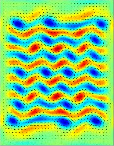
(d)

Figure 2: Rotationally symmetric equilibrium solutions (a) EQ₂ (b) EQ₀ (c) EQ₁ (d) EQ₃. Color (black arrows) indicates vorticity (velocity).

A consequence of this equivariance is that the symmetry of a rotationally invariant flow is preserved during its time evolution, i.e., the symmetry subspace $\mathcal{S}=\{{\bf u}\in\mathcal{M}\,|\,\mathcal{I}{\bf u}={\bf u}\}$ of $\mathcal{M}$ is invariant. Here, $\mathcal{M}$ represents the full state space. All ECSs and connections between them we report in this article lie in $\mathcal{S}$. Since trajectories in $\mathcal{S}$ are generally unstable, numerical errors will accumulate such that ${\bf u}(t)$ will eventually leave $\mathcal{S}$ even if ${\bf u}(0)\in\mathcal{S}$. To prevent this, we augmented the numerical integrator by projecting ${\bf u}(t)$ back into $\mathcal{S}$ after every time step Suri (2017).

III Results

As $Re$ is increased, the Kolmogorov-like flow undergoes a number of bifurcations before transitioning to weak turbulence at $Re\approx 18$ Tithof et al. (2017). At $Re\approx 22$ the flow in full state space $\mathcal{M}$ is chaotic, which was confirmed by computing the Lyapunov spectrum of a long turbulent trajectory using continuous Gram-Schmidt orthogonalization Farmer et al. (1983); Suri et al. (2018). In this dynamical regime we previously identified 31 unstable equilibria of the 2D model Suri et al. (2018). Twenty eight of these were outside of $\mathcal{S}$. Furthermore, their unstable manifolds were relatively high-dimensional in $\mathcal{M}$ (with the number of unstable directions as low as three and as high as twenty) and thus computationally forbidding to map out. Hence, we instead started our analysis with the equilibria in $\mathcal{S}$, labeled EQ₀, EQ₁, and EQ₂.

The stability properties of these equilibria and other recurrent solutions we found in $\mathcal{S}$ are summarized in Table 1. We have listed the number of unstable directions $N_{u}$ and the leading eigenvalues $\lambda$ for EQs (Floquet exponents for POs) both in the symmetry invariant subspace $\mathcal{S}$ and in the rest of state space, i.e., $\mathcal{M}\backslash\mathcal{S}$. All ECSs we computed have two or fewer unstable directions in $\mathcal{S}$, which allows their unstable manifolds to be well-approximated with a dense set of trajectories Suri et al. (2018). Note that EQ₀ and PO₀ are stable in $\mathcal{S}$. Hence, turbulence in $\mathcal{S}$ can be transient, with trajectories converging to one of these two ECSs asymptotically in time. This is indeed what numerical simulations show, as we discuss in Sect. III.6.

	$N_{u}$		$\lambda$
	$\ \mathcal{S}\$	$\mathcal{M}\backslash\mathcal{S}$	$\mathcal{S}$	$\mathcal{M}\backslash\mathcal{S}$
EQ0	0	2	$-0.004\pm 0.020i$	$0.058\pm 0.047i$
EQ1	1	2	$0.017$	$0.029$
EQ2	2	5	$0.035\pm 0.114i$	$0.022$
EQ3	1	2	$0.068$	$0.029\pm 0.029i$
PO0	0	3	$-0.003\pm 0.059i$	0.151
PO1	1	2	0.036	$0.054\pm 0.033i$
PO2	1	3	0.044	0.049
QP1	1	-	-	-

Table 1: The number of unstable directions $N_{u}$ and the leading eigenvalue(s) (Floquet exponent(s)) $\lambda$ for the recurrent solutions we computed in $\mathcal{S}$ at $Re=22.05$.

Connection(s) from an origin (ECS_-∞) to a destination (ECS_∞) lie at the intersection of the unstable manifold of ECS_-∞ and the stable manifold of ECS_∞. Since the dimensionality of stable manifolds is very high ($O(10^{5})$ in our case), we will search the low-dimensional unstable manifolds of ECSs for dynamical connections. Such unstable manifolds can be conveniently approximated by families of trajectories ${\bf u}({\bf p},t)$ that start near an ECS, where the unstable manifold is locally tangent to the linear subspace parametrized by the unstable and marginal eigenvectors of that ECS. Here, ${\bf p}$ parametrizes the family of manifold trajectories. The specifics of constructing a linear subspace, and consequently its parametrization, depend on the type of ECS (EQ or PO) as well as the dimensionality of its unstable manifold, as discussed below.

Table 1 shows that several solutions we identified have a single unstable direction in $\mathcal{S}$. The unstable manifold of such ECS is naturally divided into two halves, which correspond to the positive and negative halves of the corresponding linear subspace (see Fig. 1). We shall hereafter refer to these halves as ${\bf u}^{\pm}({\bf p},t)$. Furthermore, ${\bf u}^{\pm}({\bf p},t)$ lie on the opposite sides of the stable manifold of the ECS, which serves as a local separatrix and repels trajectories near the ECS along ${\bf u}^{+}({\bf p},t)$ or ${\bf u}^{-}({\bf p},t)$. This allows us to compute connections terminating at ECSs with one unstable direction using a simple bisection method Itano and Toh (2001). In the following sections we provide a detailed discussion of connections between various ECSs listed in Table 1.

III.1 Connections originating at EQ₂

We start our analysis with equilibrium EQ₂, which has the highest dimensional unstable manifold of all the EQs in $\mathcal{S}$. The vorticity field ($\omega=\nabla\times{\bf u}$) associated with EQ₂ is shown in Fig. 2(a). The 2D unstable manifold of EQ₂ is locally tangent to the plane spanned by the complex conjugate pair of unstable eigenvectors ${\,\bf\hat{e}}_{1},{{\,\bf\hat{e}}}_{2}={\,\bf\hat{e}}_{1}^{\ast}$ associated with $\lambda_{1,2}=\sigma\pm i\mu$, where $\sigma=0.035$ and $\mu=0.114$. To construct this 2D surface, which lies entirely in $\mathcal{S}$, we generated 360 initial conditions ${\bf u}(\theta,0)$ on a circle around EQ₂ in the plane spanned by ${{\,\bf\hat{e}}}_{1}$, ${{\,\bf\hat{e}}}_{2}$:

$${\bf u}(\theta,0)={\bf u}_{eq}+\epsilon\cos(\theta){\,\bf\hat{e}}_{1}^{\prime}+\epsilon\sin(\theta){\,\bf\hat{e}}_{2}^{\prime}.$$ (2)

Here, ${\bf u}_{eq}$ corresponds to EQ₂ and ${\,\bf\hat{e}}_{1}^{\prime}$, ${\,\bf\hat{e}}_{2}^{\prime}$ are real orthonormal vectors constructed from the real and imaginary parts of ${{\,\bf\hat{e}}}_{1}$, ${\,\bf\hat{e}}_{2}$. For numerical convenience we chose $\epsilon=0.002\cdot\|{\bf u}_{eq}\|$ and positioned the initial conditions ${\bf u}(\theta,0)$ at equal angular intervals $\Delta\theta=2\pi/360$ on the circle. Numerical integration of initial conditions ${\bf u}(\theta,0)$ generates trajectories ${\bf u}(\theta,t)$ that approximate the 2D manifold and parametrize it by $\theta$, $t$. Each manifold trajectory ${\bf u}(\theta,t)$ was computed on a temporal interval of length 25$\tau_{c}$, where $\tau_{c}=12.5$ (nondimensional time units) is the average temporal auto-correlation time Suri et al. (2018).

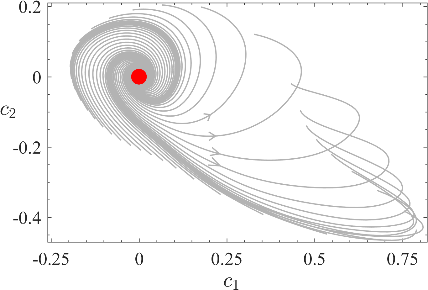
Figure 3: Trajectories ${\bf u}(\theta,t)$ (gray curves) approximating the unstable manifold of EQ₂ (red sphere). ${\bf u}(\theta,t)$ originate on a small circle around EQ₂ that lies in a plane spanned by the complex conjugate pair of unstable eigenvectors ${\,\bf\hat{e}}_{1}$ and ${\,\bf\hat{e}}_{2}$. Coordinates $c_{1},c_{2}$ are projections of ${\bf u}(\theta,t)$ onto orthonormal vectors constructed from ${\,\bf\hat{e}}_{1}$, ${\,\bf\hat{e}}_{2}$.

In the neighborhood of EQ₂, the various trajectories ${\bf u}(\theta,t)$ initially evolve spiraling outward, i.e.,

$${\bf u}(\theta,t)\approx{\bf u}_{eq}+\epsilon e^{\sigma t}\cos(\theta+\mu t){\,\bf\hat{e}}_{1}^{\prime}+\epsilon e^{\sigma t}\sin(\theta+\mu t){\,\bf\hat{e}}_{2}^{\prime}.$$ (3)

To illustrate this, we plotted a portion of the 2D unstable manifold in Fig. 3, projected onto vectors ${\,\bf\hat{e}}_{1}^{\prime}$ and ${\,\bf\hat{e}}_{2}^{\prime}$. Only one in every ten trajectories generated is shown and the segment of each trajectory ${\bf u}(\theta,t)$ plotted corresponds to $0\leq t\leq 11\tau_{c}$. Coordinates $c_{1},c_{2}$ in Fig. 3 are the normalized inner products

$$c_{k}(t)=\frac{({\bf u}(\theta,t)-{\bf u}_{eq})\cdot{\,\bf\hat{e}}^{\prime}_{k}}{D_{c}},$$ (4)

where, $D_{c}=\max_{t,t^{\prime}}\|{\bf u}(t)-{\bf u}(t^{\prime})\|=300$ is the empirically estimated maximum separation between two points on an 800$\tau_{c}$-long turbulent trajectory in $\mathcal{S}$, which defines the “diameter” of the chaotic repeller. Normalizing distances with $D_{c}$ ensures that points separated by nearly unit distance in the low-dimensional projection are very far apart in full state space. Notice that, farther away from EQ₂ ($|c_{1}|,|c_{2}|>0.2$) the shape of ${\bf u}(\theta,t)$ becomes fairly complicated due to the nonlinearity of the governing equation (1).

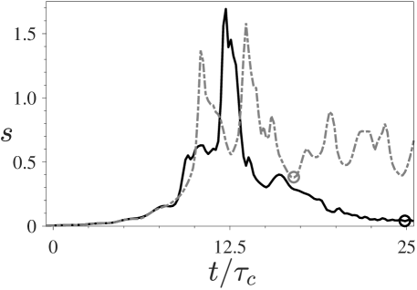
Figure 4: State space speeds $s(\theta,t)$ along two trajectories in the unstable manifold of EQ₂ that exhibit contrasting dynamics. Solid (dashed) curve is speed along a trajectory that approaches (does not approach) an equilibrium closely after leaving the neighborhood of EQ₂. The lowest speed $s_{m}(\theta)=\min_{t}s(\theta,t)$ for $t/\tau_{c}\in[10,25]$ for each curve is marked using an open circle.

It is not known a priori which ${\bf u}(\theta,t)$ approach an ECS (EQ or PO) closely after leaving the neighborhood of EQ₂. Previously, Gibson et al.aGibson et al. (2008) and Halcrow et al.aHalcrow et al. (2009) inferred possible dynamical connections by inspecting low-dimensional state space projections. In contrast, Riols et al.aRiols et al. (2013) analyzed time-series of (magnetic) energy and identified close passes to POs using intervals with “periodic” behavior. Both these techniques, however, require visual inspection and detecting signatures of dynamical connections cannot be automated. In this study we tested two methods to detect signatures of dynamical connections that do not require laborious visual inspection. The method employed for detecting connections that terminate at EQs proved very effective and is discussed next. A method for detecting connections to POs using recurrence analysis Duguet et al. (2008a) is discussed in Appendix B.

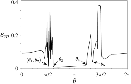
Figure 5: Minimum state space speed $s_{m}(\theta)=\min_{t}s(\theta,t)$ along each trajectory ${\bf u}(\theta,t)$ in the 2D unstable manifold of EQ₂. Trajectories corresponding to $s_{m}\ll 1$ are possible dynamical connections from EQ₂ to an equilibrium.

For each trajectory ${\bf u}(\theta,t)$ in the unstable manifold of EQ₂, we computed the normalized instantaneous state space speed $s(\theta,t)$, which we define as Suri et al. (2017, 2018):

$$s(\theta,t)=\frac{\tau_{c}}{\|{\bf u}(\theta,t)\|}\left\|\partial_{t}{\bf u}(\theta,t)\right\|.$$ (5)

Since $\partial_{t}{\bf u}=0$ ($s=0$) for any EQ, $s(\theta,t)\ll 1$ indicates that a trajectory ${\bf u}(\theta,t)$ in state space is near an EQ Suri et al. (2017); Neelavara et al. (2017). In the physical space, this corresponds to the evolution of the flow dramatically slowing down. Figure 4 shows, as examples, the speed plots for two different manifold trajectories ${\bf u}(\pi/2,t)$ and ${\bf u}(3\pi/2,t)$. Clearly, ${\bf u}(\theta,t)$ lie in the linear neighborhood of EQ₂ for $0<t\lesssim 10\tau_{c}$ ($s\ll 1$) and $s(\theta,t)$ grows exponentially according to equation (3). After this initial transient, however, dynamics described by various trajectories can be qualitatively very different. For instance, the shape of $s(3\pi/2,t)$ (gray curve) suggests that ${\bf u}(3\pi/2,t)$ displays turbulent evolution. In contrast, $s(\pi/2,t)$ (black curve) suggests that ${\bf u}({\pi/2},t)$ approaches an EQ closely after a brief turbulent excursion.

(a)

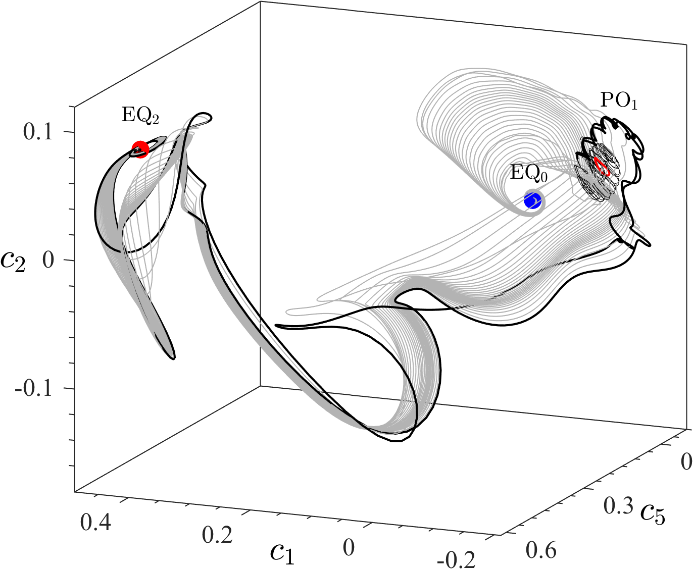
(b)

Figure 6: Heteroclinic connections from EQ₂ to various ECSs. (a) A connection (gray curve) to EQ₀ that belongs to the family DC₁ and an isolated connection DC₃ (black curve) to EQ₁ (b) Family of connections DC₂ (gray curves) that terminate at EQ₀ and isolated connections DC₆, DC₇ (black curves) to PO₁.

Hence, to test if a trajectory ${\bf u}(\theta,t)$ approaches an EQ after it departs from the neighborhood of EQ₂, we computed the minimum speed $s_{m}(\theta)=\min_{t}s(\theta,t)$ for $10\tau_{c}\leq t\leq 25\tau_{c}$, which is shown in Fig. 5. The low values of $s_{m}(\theta)$ for $\theta\in\left(\theta_{1},\theta_{2}\right)$, $\theta\in\left(\theta_{3},\theta_{4}\right)$, and $\theta={\theta_{5}}$ strongly suggest that the corresponding trajectories ${\bf u}(\theta,t)$ closely shadow either heteroclinic or homoclinic connections from EQ₂ to other EQs. In Fig. 5, the uncertainty in $\theta$ is limited by the angular resolution $\Delta\theta$ in the initial conditions ${\bf u}(\theta,0)$. Consequently, to compute exact dynamical connections, the estimates for $\theta$ may require refinement in some cases. The labels $\theta_{1}$ through $\theta_{5}$ in Fig. 5 correspond to these refined values. Lastly, $s_{m}(\theta)>0$ even for trajectories ${\bf u}(\theta,t)$ that correspond exactly to dynamical connections. This is because, minima in the $s(\theta,t)$ are computed on a finite temporal interval, while dynamical connections converge ($s_{m}=0$) to the destination EQs only in infinite time.

The destination EQs that different dynamical connections approach were computed using a Newton solver Saad and Schultz (1986); Kelley (2003); Mitchell (2013) initialized with the flow field ${\bf u}(\theta,t)$ at the instant when $s(\theta,t)=s_{m}(\theta)$. For $\theta\in\left(\theta_{1},\theta_{2}\right)$ and $\theta\in(\theta_{3},\theta_{4})$ the solver converged to EQ₀, which is a stable node in $\mathcal{S}$. For $\theta=\theta_{5}$ the solver converged to EQ₁, which is a saddle with one unstable direction in $\mathcal{S}$. The flow fields corresponding to EQ₀ and EQ₁ are shown in Figs. 2(b) and 2(c). Dimensional arguments (discussed in Sect. III.5) suggest that connections from EQ₂ to EQ₀ should comprise a one-parameter family forming a two-dimensional manifold, just like those in the interval $(\theta_{3},\theta_{4})$. However, the difference $\theta_{2}-\theta_{1}$ is smaller than the resolution $\Delta\theta$ in case of the interval $(\theta_{1},\theta_{2})$. Consequently, $\theta_{1}$, $\theta_{2}$ cannot be distinguished in Fig. 5. Hereafter, we will refer to $\theta$ in this narrow interval $(\theta_{1},\theta_{2})$ collectively as $\theta_{n}$. The wide interval $(\theta_{3},\theta_{4})$ will be referred to as $\theta_{w}$. Lastly, to confirm that the dynamical connections originating at EQ₂ indeed terminate at either EQ₀ or EQ₁, we need to make sure that the distance

$$D_{0}=\min\limits_{t}\frac{\|{\bf u}(\theta,t)-{\bf u}_{eq}\|}{D_{c}},$$ (6)

vanishes in the limit $t\to\infty$. Here, ${\bf u}_{eq}$ is the velocity field corresponding to the destination EQ. For all connections reported in this study, we chose $D_{0}<0.005$ as the criterion for convergence.

Let us start our analysis with the trajectories ${\bf u}(\theta_{n},t)$ and ${\bf u}(\theta_{w},t)$ that approach the equilibrium EQ₀ which is stable in $\mathcal{S}$. The eigenvalues of weakly contracting modes of EQ₀ are $\lambda_{1,2}=-0.004\pm 0.020i$, $\lambda_{3,4}=-0.012\pm 0.42i$. Consequently, most nearby trajectories in $\mathcal{S}$ converge to EQ₀ at a rate determined by the real part of $\lambda_{1}$ (${\lambda_{1}}$). Hence, we computed trajectories ${\bf u}(\theta_{n},t)$ and ${\bf u}(\theta_{w},t)$ for an interval of duration $350\tau_{c}\gg 1/\lambda_{1}\approx 10\tau_{c}$. At the end of numerical integration both ${\bf u}(\theta_{n},t)$ and ${\bf u}(\theta_{w},t)$ approached EQ₀ to within a distance $D_{0}<10^{-8}$, confirming that we have indeed found heteroclinic connections from EQ₂ to EQ₀. Hereafter, we shall refer to these dynamical (heteroclinic) connections corresponding to ${\bf u}(\theta_{n},t)$ and ${\bf u}(\theta_{w},t)$ as DC₁ and DC₂, respectively.

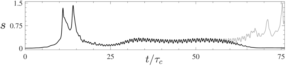
Figure 7: State space speed along trajectories ${\bf u}(\theta_{4}^{-},t)$ (black) and ${\bf u}(\theta_{4}^{+},t)$ (gray) that separate after shadowing a periodic orbit.

A connection from the family DC₁ is shown (gray curve) in Fig. 6(a) and thirty connections from DC₂ that are equally spaced on the interval $(\theta_{3},\theta_{4})$ are shown in Fig. 6(b). Both figures show the projection of state space onto an orthogonal basis constructed from the stable eigenvectors ${\,\bf\hat{e}}_{1}$, ${\,\bf\hat{e}}_{2}$, and ${\,\bf\hat{e}}_{5}$ of EQ₀. The vectors ${\,\bf\hat{e}}_{1}$, ${\,\bf\hat{e}}_{2}$ were chosen to visualize asymptotic dynamics along the connections terminating at EQ₀. The vector ${\,\bf\hat{e}}_{5}$ was chosen because trajectories ${\bf u}(\theta,t)$ far away from EQ₀ have large components along this direction. We note that, unless mentioned otherwise, these modes are used for all state space projections in this article.

In Fig. 6, both DC₁ and DC₂ converge to EQ₀ spiraling inwards, almost entirely confined to the $c_{1}-c_{2}$ plane. This is a consequence of the large separation between the real values of $\lambda_{1,2}$ and $\lambda_{3,4}$ which makes ${\,\bf\hat{e}}_{1}$, ${\,\bf\hat{e}}_{2}$ the only dynamically relevant eigenvector pair near EQ₀. Another interesting feature of Fig. 6(b) is that DC₂ initially forms a flat strip bounded by manifold trajectories ${\bf u}(\theta_{3},t)$ and ${\bf u}(\theta_{4},t)$ (black curves). However, farther away from EQ₂, this strip widens and folds such that ${\bf u}(\theta_{3},t)$ and ${\bf u}(\theta_{4},t)$ come close to each other, trace loops which are strikingly similar in shape, and eventually merge (see inset in Fig. 8). This is not an artifact of low-dimensional projection of the state space. As we explain in the following section, the black trajectories in Fig. 6(b) correspond to heteroclinic connections from EQ₂ to a different ECS (PO₁).

Unlike DC₁ and DC₂, the trajectory ${\bf u}(\theta_{5},t)$ approaches the solution EQ₁ which has one unstable direction (cf. Table 1). Since the stable/unstable manifolds of EQ₁ guide the evolution of trajectories in its neighborhood, we explored their geometry to compute the connection from EQ₂ to EQ₁. Trajectories ${\bf u}(\theta,t)$ for $\theta\approx\theta_{5}$ that approach EQ₁ should subsequently depart following its unstable manifold, which coincides with a pair of trajectories

$${\bf u}^{\pm}(t)={\bf u}_{eq}\pm\epsilon e^{\lambda_{1}t}{\,\bf\hat{e}}_{1},$$ (7)

in the linear neighborhood of EQ₁ (cf. Fig. 1). Here, ${\,\bf\hat{e}}_{1}$ is the unstable eigenvector of EQ₁ and $\epsilon>0$ is some small constant. In particular, we found a pair of adjacent trajectories ${\bf u}(\theta,t)$ and ${\bf u}(\theta+\Delta\theta,t)$ with $\theta\approx\theta_{5}$ approach EQ₁ and depart its neighborhood in opposite directions shadowing ${\bf u}^{+}(t)$ and ${\bf u}^{-}(t)$, respectively. Hence, a heteroclinic connection DC₃ from EQ₂ to EQ₁ lies between these two trajectories, i.e., in the stable manifold of EQ₁.

The projection of DC₃ (black curve) is shown in Fig. 6(a). It was computed by refining the estimate for $\theta_{5}$ to within $\delta\theta=2^{-12}\Delta\theta$ using bisection Itano and Toh (2001); Gibson et al. (2008); Halcrow et al. (2009). This refinement reduced the separation between ${\bf u}(\theta_{5},t)$ and EQ₁ to $D_{0}=0.002$ (cf. equation (6)). Further refinement in $\theta$ did not significantly reduce $D_{0}$ since numerical noise on ${\bf u}(\theta_{5},t)$ amplifies rapidly in the direction of unstable eigenvector $\pm{\,\bf\hat{e}}_{1}$ of EQ₁. This behavior stems from the strong asymmetry in the real parts of unstable ($\lambda_{1}=0.017$) and weakly stable ($\lambda_{2,3}=-0.003\pm 0.109i$) eigenvalues of EQ₁. Nevertheless, a better accuracy can be achieved by employing multi-shooting van Veen et al. (2011) or approximating DC₃ as a piece-wise continuous solution Toh and Itano (2003). Using the latter technique allowed us to decrease $D_{0}$ to less than $10^{-6}$. Lastly, equation (7) governs the evolution of trajectories in the unstable manifold of EQ₁ only in its linear neighborhood. Farther away, both ${\bf u}^{\pm}(t)$ display turbulent evolution for $t\gg 100\tau_{c}$ and eventually approach EQ₀. Hence these two trajectories define (long) heteroclinic connections (DC₄, DC₅) from EQ₁ to EQ₀.

III.2 Dynamics Near PO₁ and EQ₃

While trajectories ${\bf u}(\theta,t)$ for $\theta\in(\theta_{3},\theta_{4})$ quickly converge to EQ₀, trajectories just outside this interval exhibit qualitatively different dynamics; this can be inferred from $s_{m}$ changing abruptly at $\theta_{3}$ and $\theta_{4}$. This qualitative difference suggests that trajectories ${\bf u}(\theta_{3},t)$ and ${\bf u}(\theta_{4},t)$ play the role of separatrices on the unstable manifold of EQ₂ and hence lie in the stable manifold of another ECS. In case of ${\bf u}(\theta_{4},t)$, for example, we found this ECS by inspecting the two trajectories ${\bf u}(\theta_{4}^{-},t)$ and ${\bf u}(\theta_{4}^{+},t)$ obtained as a result of successive bisections; here $\theta_{4}^{\pm}=\theta_{4}\pm\delta\theta$ with $\delta\theta=2^{-12}\Delta\theta$. The corresponding state space speed plots are shown in Fig. 7, which suggest that ${\bf u}(\theta_{4}^{\pm},t)$ evolve almost indistinguishably for about $55\tau_{c}$ and subsequently separate. For $t/\tau_{c}\in[30,55]$ the state space speed oscillates with a period of approximately $1.4\tau_{c}$, suggesting that ${\bf u}(\theta_{4}^{\pm},t)$ shadow a periodic orbit during this interval.

Using the flow field corresponding to ${\bf u}(\theta_{4}^{+},t)$ at $t/\tau_{c}=55$ as an initial condition into a Newton solver, we indeed found an unstable periodic orbit PO₁ with a period $T=1.32\tau_{c}$. A similar refinement using bisection showed that trajectories at $\theta_{3}^{\pm}=\theta_{3}\pm\delta\theta$ also approach PO₁ and separate after shadowing it for an extended period of time (the corresponding speed plots are not shown). Figure 8 shows the state space projection of ${\bf u}(\theta_{4}^{\pm},t)$ and ${\bf u}(\theta_{3}^{\pm},t)$ approaching PO₁, shadowing it closely (inset), and subsequently leaving its neighborhood. The projection coordinates here are the same as in Fig. 6, but the viewing angle is different. Lastly, the result that ${\bf u}(\theta_{3}^{\pm},t)$ and ${\bf u}(\theta_{4}^{\pm},t)$ approach PO₁ is consistent with the folding of DC₂ shown in Fig. 6(b).

PO₁ has a single real unstable direction in $\mathcal{S}$ with an associated Floquet exponent $\lambda_{1}=0.036$ (cf. Table 1). Hence, the departure of ${\bf u}(\theta_{3}^{\pm},t)$ and ${\bf u}(\theta_{4}^{\pm},t)$ from the neighborhood of PO₁ is guided by its unstable manifold, which is two-dimensional since it is associated with a PO which is itself one-dimensional. This 2D unstable manifold can be constructed by evolving initial conditions Riols et al. (2013)

$${\bf u}^{\pm}(\eta,0)={\bf u}_{po}\pm\epsilon e^{\lambda_{1}\eta}{\,\bf\hat{e}}_{1},$$ (8)

where ${\bf u}_{po}$ is a reference point on PO₁, ${\,\bf\hat{e}}_{1}$ is the Floquet vector at ${\bf u}_{po}$, $\epsilon>0$ is sufficiently small (we chose $\epsilon=0.001\cdot\|{\bf u}_{po}\|$), and $\eta\in(0,T]$ parametrizes different initial conditions. A total of $720$ initial conditions, equally spaced in $\eta$, were generated and the corresponding trajectories ${\bf u}^{\pm}(\eta,t)$ were computed on an interval of length $35\tau_{c}$ to approximate the manifold. We found that trajectories ${\bf u}^{+}(\eta,t)$ uneventfully converge to EQ₀ while ${\bf u}^{-}(\eta,t)$ display turbulent evolution after leaving the neighborhood of PO₁. To illustrate this, we plotted in Fig. 8 a pair of trajectories ${\bf u}^{\pm}(\eta,t)$ (red dashed curves) evolving in opposite directions.

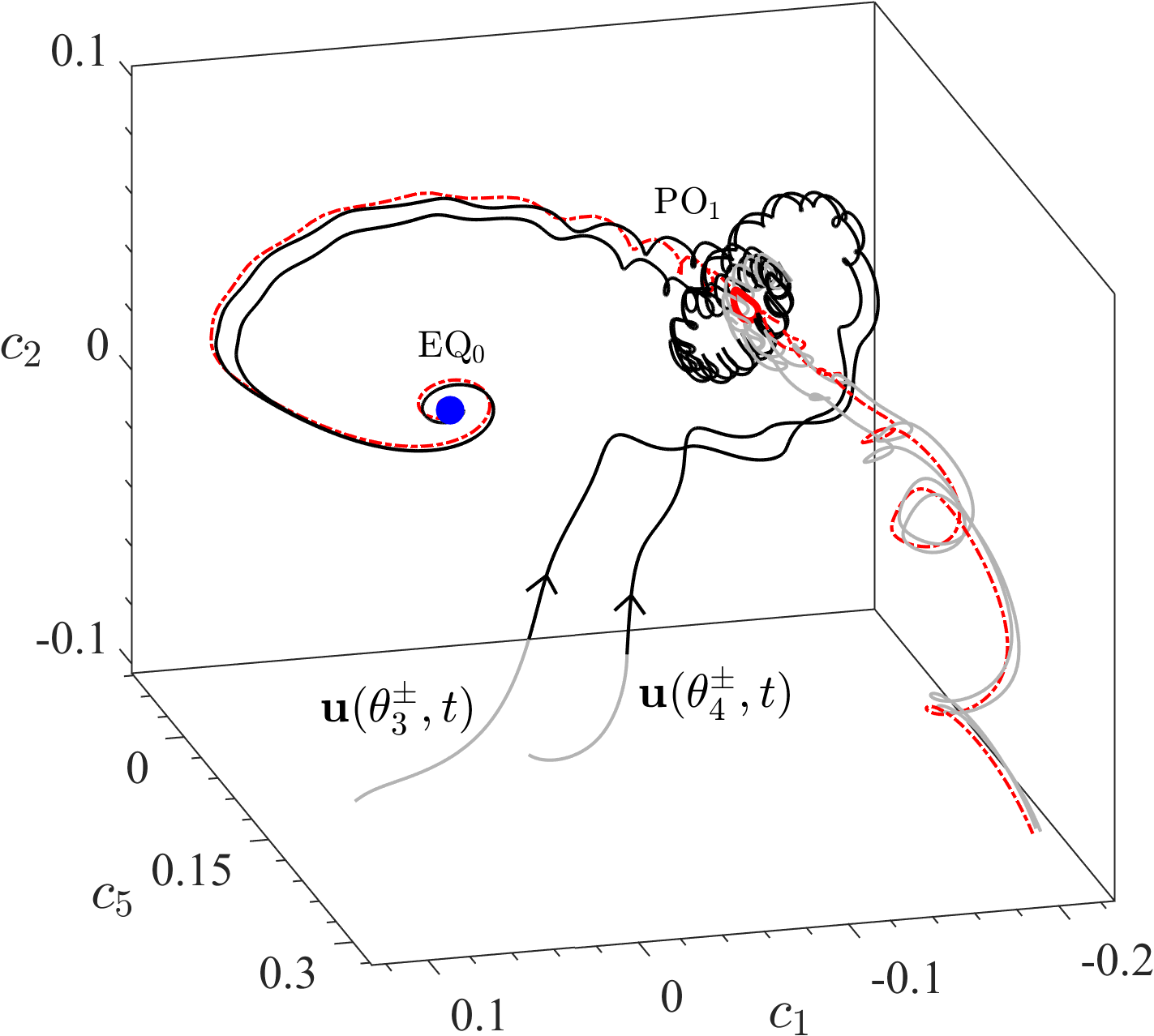
Figure 8: Geometry of state space around PO₁. Trajectories ${\bf u}(\theta_{4}^{\pm},t)$ approach PO₁ indistinguishably, but depart from its neighborhood in opposite directions (inset) guided by the manifold trajectories ${\bf u}^{\pm}(\eta,t)$ (dashed red curves). ${\bf u}(\theta_{4}^{-},t)$ (black curve) converges to EQ₀ and ${\bf u}(\theta_{4}^{+},t)$ (gray curve) becomes turbulent. Similar behavior is manifested by ${\bf u}(\theta_{3}^{\mp},t)$.

Since PO₁ has a single unstable direction, its stable manifold divides the state space in the neighborhood of PO₁ into two halves Avila et al. (2013). We found that trajectories ${\bf u}(\theta_{3}^{+},t)$ and ${\bf u}(\theta_{4}^{-},t)$ smoothly converge to EQ₀ after approaching PO₁ and hence lie on one (the same) side of the stable manifold. Meanwhile ${\bf u}(\theta_{3}^{-},t)$ and ${\bf u}(\theta_{4}^{+},t)$ display turbulent excursions and hence lie on the opposite side of the stable manifold, as shown in Fig. 8. Therefore, there exist two heteroclinic connections from EQ₂ to PO₁ sandwiched between ${\bf u}(\theta_{3}^{\pm},t)$ (DC₆) and ${\bf u}(\theta_{4}^{\pm},t)$ (DC₇), that lie on the stable manifold and asymptotically converge to PO₁. Just like in the case of DC₃, simple shooting cannot be employed to compute DC₆ and DC₇ in their entirety since they are very unstable. Nevertheless, for sufficient refinement in $\theta$, the trajectories ${\bf u}(\theta_{3}^{\pm},t)$ and ${\bf u}(\theta_{4}^{\pm},t)$ approximate DC₆ and DC₇, respectively, reasonably accurately (cf. Fig. 6(b)). This was tested by computing the smallest distance between ${\bf u}(\theta,t)$ and PO₁

$$D_{1}=\min\limits_{t,\eta}\frac{\|{\bf u}(\theta,t)-{\bf u}_{po}(\eta)\|}{D_{c}},$$ (9)

where ${\theta}=\theta_{3}^{\pm}$ or $\theta_{4}^{\pm}$ and ${\bf u}_{po}(\eta)$ are states along PO₁ parametrized by $\eta\in(0,T]$. We found that $D_{1}<0.005$ in both cases.

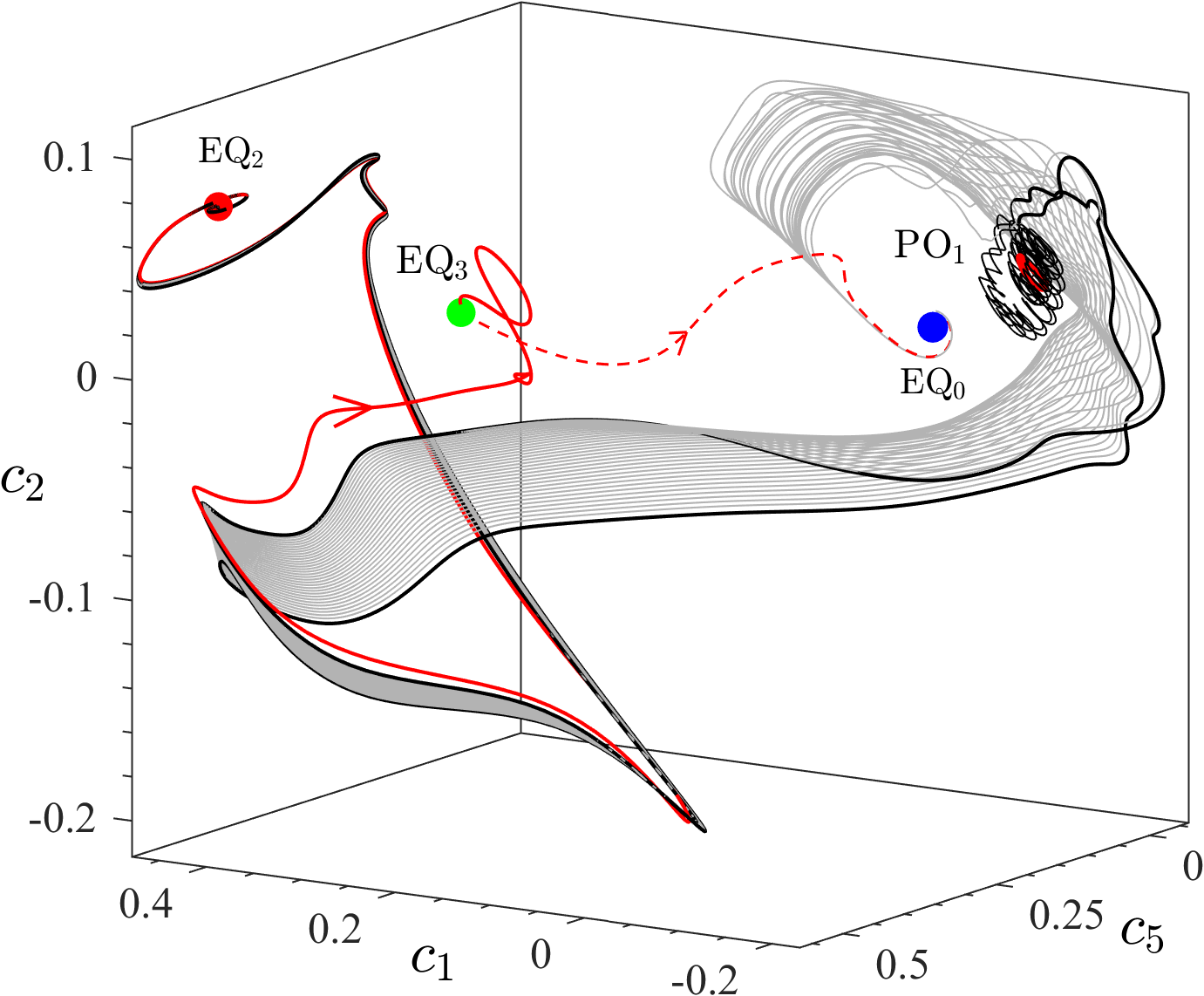
Figure 9: Heteroclinic connections DC₈, DC₉ (black curves) from EQ₂ to PO₁ that sandwich the family of connections DC₁ (gray curves) from EQ₂ to EQ₀. The solid (dashed) red curve is the connection DC₁₀ (DC₁₁) from EQ₂ to EQ₃ (EQ₃ to EQ₀).

Fig. 8 shows a toroidal structure traced out by ${\bf u}(\theta_{4}^{\pm},t)$ and ${\bf u}(\theta_{3}^{\pm},t)$ as these trajectories approach PO₁ along its stable manifold. A magnified view of this region shown in the inset illustrates the complicated shape of the manifold. The numerous small loops correspond to the fast constant amplitude oscillation along PO₁. In contrast, the large spiral corresponds to a slowly decaying oscillation described by the stable Floquet vectors ${\,\bf\hat{e}}_{2}$, ${\,\bf\hat{e}}_{3}$ of PO₁ with exponents $\lambda_{2,3}=-0.0044\pm 0.0264i$. The characteristic time associated with this slow oscillation is $2\pi/0.0264\approx 20\tau_{c}$ and manifests itself in the weak modulation of the state space speed during the interval $t\in[30\tau_{c},50\tau_{c}]$ in Fig. 7.

As mentioned earlier, based on dimensional arguments, DC₁ should be a 2D manifold which corresponds to a one-parameter family of trajectories connecting EQ₂ to EQ₀. Since the corresponding interval $\theta_{n}$ is very narrow, $\theta_{2}-\theta_{1}<\Delta\theta$, we resampled a wider interval of width $2\Delta\theta$ that includes $\theta_{n}$ using 100 equally spaced initial conditions. This refinement showed that $\theta_{2}-\theta_{1}\approx 0.5\Delta\theta$ and all trajectories inside this interval converge to EQ₀, i.e., DC₁ is indeed a 2D manifold. Thirty trajectories from DC₁ are shown (as gray curves) in Fig. 9. The projection coordinates and the viewing angle are the same as in Fig. 6. As in the case of DC₂, the trajectories ${\bf u}(\theta_{1},t)$ and ${\bf u}(\theta_{2},t)$ at the left and right edges of DC₁ are separatrices on the 2D unstable manifold of EQ₂. Using bisection, we identified that both ${\bf u}(\theta_{1},t)$ and ${\bf u}(\theta_{2},t)$ approach PO₁ closely ($D_{1}<0.005$) and well-approximate heteroclinic connections DC₈, DC₉ from EQ₂ to PO₁ shown (as black curves) in Fig. 9.

The refinement in initial conditions around $\theta_{n}$ also revealed that a few trajectories ${\bf u}(\theta,t)$ for $\theta_{1}-\Delta\theta<\theta<\theta_{1}$ approach an unstable equilibrium EQ₃. The flow field corresponding to EQ₃ is shown in Fig. 2(d). EQ₃ has a single unstable direction in $\mathcal{S}$ and its unstable manifold is one-dimensional, similar to EQ₁ (see Fig. 1). Also, we found that a pair of adjacent trajectories from EQ₂ approach EQ₃ and subsequently depart in opposite directions. Hence, using bisection we computed the heteroclinic connection DC₁₀ from EQ₂ to EQ₃ (solid red curve in Fig. 9). Additionally, we also found that one of the manifold trajectories of EQ₃ uneventfully converges to EQ₀. This connection (DC₁₁) is also shown (as dashed red curve) in Fig. 9. The manifold trajectory from EQ₃ evolving in the opposite direction, however, also converged to EQ₀ after a long turbulent excursion and hence corresponds to another connection (DC₁₂). This qualitative difference in dynamics on the two sides of the stable manifold of EQ₃ is not observed in case of EQ₁. As mentioned previously, both trajectories in the 1D unstable manifold of EQ₁ display long turbulent excursions.

III.3 Connections originating at PO₁

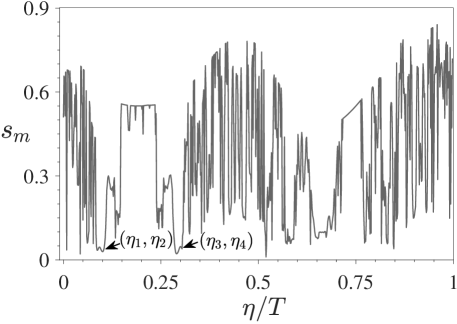
Figure 10: Minimum state space speed (black curve) $s_{m}$ along trajectories ${\bf u}^{-}(\eta,t)$ in the 1D unstable manifold of PO₁. $\eta\in[0,T)$ parametrizes points along PO₁.

As we have established, all trajectories ${\bf u}^{+}(\eta,t)$ from PO₁ quickly converge to EQ₀ (cf. Fig. 8). These trajectories constitute a one-parameter family of heteroclinic connections from PO₁ to EQ₀ which form a 2D manifold DC₁₃. The union of DC₆ and DC₇ forms a 1D boundary of the union of the 2D manifolds DC₂ and DC₁₃. Similarly, the union of DC₈ and DC₉ forms a 1D boundary of the union of 2D manifolds DC₁ and DC₁₃.

Unlike ${\bf u}^{+}(\eta,t)$, the trajectories ${\bf u}^{-}(\eta,t)$ display turbulent excursions after departing from the neighborhood of PO₁. Hence, we tested whether for some $\eta$ they approach other ECSs, as in the case of trajectories ${\bf u}(\theta,t)$ in the 2D unstable manifold of EQ₂ (cf. Sect. III.1). Since ${\bf u}^{-}(\eta,t)$ is also a one-parameter family of trajectories, we followed the procedure discussed in Sect. III.1 to search for signatures of dynamical connections originating at PO₁.

To begin, we computed the state space speed $s(\eta,t)$ for each trajectory ${\bf u}^{-}(\eta,t)$ (e.g., Fig. 16 in Appendix B) and calculated $s_{m}(\eta)=\min_{t}s(\eta,t)$ for $t/\tau_{c}\in[{15,35}]$. From the plot of $s_{m}$ versus $\eta$, shown in Fig. 10, we identified about 20 trajectories with $s_{m}\ll 1$ as possible dynamical connections. Surprisingly, all these trajectories converged to EQ₀. This was tested by extending the corresponding ${\bf u}^{-}(\eta,t)$ until the separation from EQ₀ decreased to $D_{0}<0.01$. Since a detailed analysis of dynamics along all of these trajectories is not feasible, we limit the discussion to the families of connections DC₁₄ that correspond to the interval $(\eta_{1},\eta_{2})$ marked in Fig. 10.

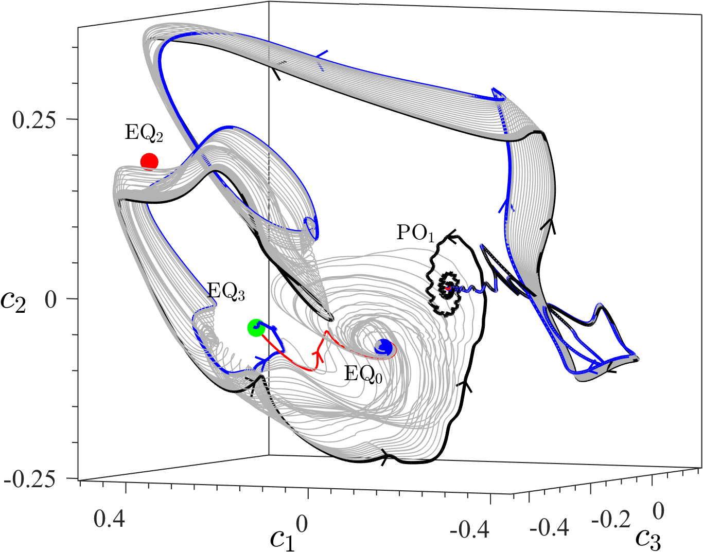
Figure 11: Family of heteroclinic connections (DC₁₄, gray curves) from PO₁ to EQ₀. The black curve is a homoclinic orbit of PO₁ (DC₁₅) and the blue curve is a heteroclinic connections from PO₁ to EQ₃ (DC₁₆). The red curve is DC₁₁ from EQ₃ to EQ₀.

About thirty trajectories (gray curves) from the family DC₁₄ are shown in Fig. 11 which, unlike all other figures, employs a projection of the state space onto an orthonormal basis constructed from Floquet vectors ${\,\bf\hat{e}}_{1}$ (unstable, real) and ${\,\bf\hat{e}}_{2},\,{\,\bf\hat{e}}_{3}$ (stable, complex conjugate pair) of PO₁. Trajectories in DC₁₄ leave the neighborhood of PO₁ along ${\bf e}_{1}$. After a brief turbulent excursion, they visit the neighborhood of EQ₂ and finally converge to EQ₀. An interesting feature of Fig. 11 is that several trajectories in DC₁₄ appear to visit the neighborhood of PO₁ enroute to EQ₀. This raises the question of whether a homoclinic orbit ${\bf u}^{-}(\eta,t)$ of PO₁ exists near the interval $(\eta_{1},\eta_{2})$. Since PO₁ has one unstable direction, a homoclinic orbit should be sandwiched between trajectories that show qualitatively different dynamics Burak Budanur et al. (2018). Such a behavior is indeed observed for trajectories near $\eta_{1}$ and $\eta_{2}$ where $s_{m}$ changes abruptly. Using bisection, we refined the estimate for $\eta_{2}$ and found that ${\bf u}^{-}(\eta_{2},t)$ indeed approaches PO₁ very closely (within $D_{1}<0.005$) and therefore well-approximates a homoclinic connection DC₁₅ shown (black curve) in Fig. 11. The projection used in this figure allows visualization of the asymptotic dynamics along DC₁₅ for both early times (on the unstable manifold of PO₁) and late times (on the stable manifold of PO₁). Refining the estimate for $\eta_{1}$ using bisection revealed that ${\bf u}^{-}(\eta_{1},t)$ instead converges to EQ₃ (with $D_{0}=5\times 10^{-4}$), approximating a heteroclinic connection DC₁₆ (blue curve in Fig. 11).

We found that trajectories ${\bf u}^{-}({\eta,t})$ in the interval marked $(\eta_{3},\eta_{4})$ in Fig. 10 also converge to EQ₀, after a brief turbulent excursion. These trajectories constitute a one-parameter family of connections DC₁₇ from PO₁ to EQ₀. Using bisection, we identified that ${\bf u}^{-}(\eta_{3},t)$ is another homoclinic orbit (DC₁₈) of PO₁ while ${\bf u}^{-}(\eta_{4},t)$ is a heteroclinic connection (DC₁₉) from PO₁ to EQ₃. The shapes of DC₁₇, DC₁₈, and DC₁₉ are very similar to that of DC₁₄, DC₁₆, and DC₁₅, respectively, and hence are not shown. Note that we have so far inspected state space along manifold trajectories to detect signatures of dynamical connections to EQs. An alternative metric, which allows one to identify signatures of close passes to both EQs and POs is discussed in more detail in Appendix B. Trajectories ${\bf u}^{-}({\eta,t})$ originating at PO₁ are analyzed using both metrics and the results are compared in Fig. 16.

III.4 Connections originating at PO₂

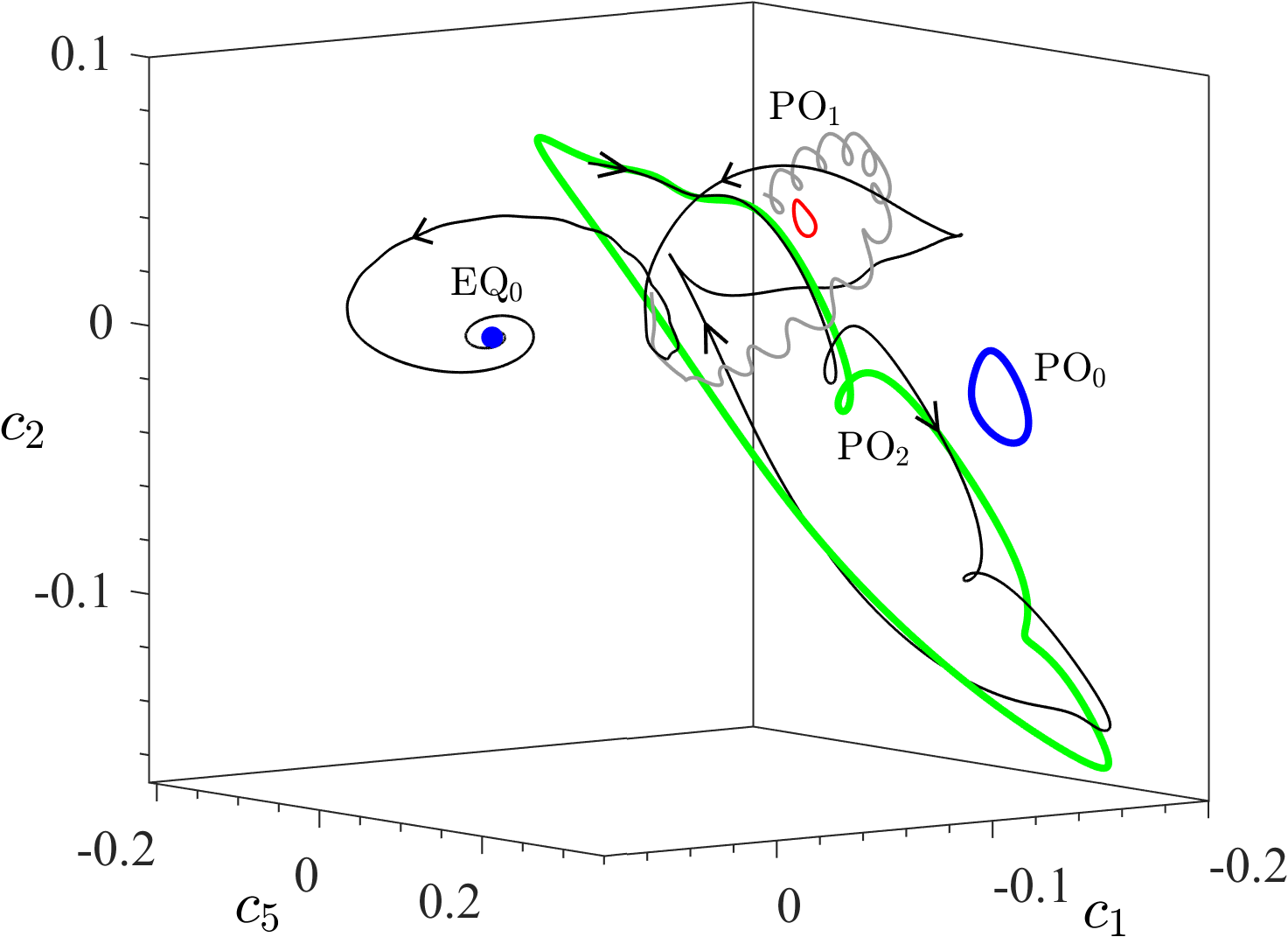
Figure 12: Heteroclinic connections from PO₂ (green loop) to EQ₀ (DC₂₀, black curve) and PO₁ (DC₂₁, gray curve). DC₂₁ eventually converges to PO₁ tracing out a helical path similar to that shown in Fig. 8.

Visual inspection of state space speed and recurrence plots (e.g., Fig. 16) revealed that some turbulent trajectories ${\bf u}^{-}(\eta,t)$ from PO₁ shadow an unstable periodic orbit PO₂. This orbit, which we computed using a Newton solver, has a period $T=4.61\tau_{c}$ and is only moderately repelling in $\mathcal{S}$; its leading Floquet exponents are $\lambda_{1}=0.044$, $\lambda_{2,3}=-0.019\pm 0.016i$. However, we did not find evidence of a short heteroclinic connection from PO₁ to PO₂, i.e., ${\bf u}^{-}(\eta,t)$ for $t/\tau_{c}\in(15,35)$ did not approach PO₂ very closely. Hence, we tested whether a connection instead exists from PO₂ to PO₁.

The 2D unstable manifold of PO₂ is composed of two sets of trajectories ${\bf u}^{\pm}(\xi,t)$ that start from initial conditions ${\bf u}^{\pm}(\xi,0)$ constructed using equation (8). Here, $\xi$ (instead of $\eta$) parametrizes states along PO₂ as well as the trajectories ${\bf u}^{\pm}(\xi,t)$. Unlike the unstable manifold of PO₁, we found that trajectories in both ${\bf u}^{+}(\xi,t)$ and ${\bf u}^{-}(\xi,t)$ display turbulent evolution. Hence, we analyzed ${\bf u}^{-}(\xi,t)$ as well as ${\bf u}^{+}(\xi,t)$ for signatures of dynamical connections; the plot of $s_{m}(\xi)$ for each set is included as Fig. S1 in the supplementary material. Inspecting state space speed (as well as recurrence) plots for each trajectory and following the procedure outlined in the previous sections, we identified a family of heteroclinic connections from PO₂ to EQ₀ (DC₂₀) and two isolated connections to PO₁ (DC₂₁, DC₂₂) that lie at the boundary of DC₂₀. A connection from the family DC₂₀ (black curve) and the isolated connection DC₂₁ (gray curve) are shown in Fig. 12. The projection coordinates here are the same as in Fig. 8 and the viewing angle is similar. We note that DC₂₀, DC₂₁, and DC₂₂ (not shown) approach their respective destinations quickly after leaving the neighborhood of PO₂.

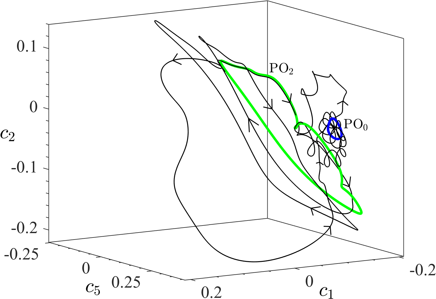
Figure 13: Heteroclinic connection DC₂₃ from PO₂ (green loop) to PO₀ (blue loop). The inset shows the unstable quasi-periodic orbit QP₁ (red curve) that lies near stable PO₀.

We also found that a narrow band of trajectories ${\bf u}^{+}(\xi,t)$ for $\xi\in(\xi_{1},\xi_{2})$ from PO₂ approach a periodic orbit PO₀ shown in Fig. 12. PO₀ has a period $T=1.22\tau_{c}$ and is stable in $\mathcal{S}$, with its leading Floquet exponent being $\lambda_{1,2}=-0.0026\pm 0.059i$. Hence, a one-parameter family of connections DC₂₃ from PO₂ to PO₀ was computed by evolving ${\bf u}^{+}(\xi,t)$ for $\xi\in(\xi_{1},\xi_{2})$ for $t\approx 400\tau_{c}$. The state space projection of a trajectory from the family DC₂₃ is shown in Fig. 13. Since PO₀ is stable in $\mathcal{S}$, DC₂₃ is a 2D manifold and trajectories that correspond to the left ($\xi_{1}$) and right ($\xi_{2}$) edges separate trajectories converging to PO₀ from those which become turbulent. Using bisection, we found that both ${\bf u}^{+}(\xi_{1},t)$, ${\bf u}^{+}(\xi_{2},t)$ approach a 2-torus representing an unstable quasi-periodic orbit (QPO) QP₁ shown in Fig. 13 (inset). Hence, ${\bf u}^{+}(\xi_{1},t)$, ${\bf u}^{+}(\xi_{2},t)$ correspond to connections DC₂₄, DC₂₅ from PO₂ to QP₁.

The state space speed for ${\bf u}^{+}(\xi_{1},t)$ clearly shows dynamics with two different frequencies over a time interval $70\tau_{c}$ (Fig. S2 in supplementary material). Computing recurrence plots for this segment of ${\bf u}^{+}(\xi_{1},t)$, we estimated that the periods associated with large and small loops of QP₁ are $T_{1}/\tau_{c}=12.21\pm 0.018$ and $T_{2}/\tau_{c}=1.21\pm 0.05$, respectively. Since the ratio $T_{1}/T_{2}\approx 10.05$ is close to an integer, we also used the Newton-Krylov solver to test whether QP₁ is instead a periodic orbit with period $T\approx T_{1},\,2T_{1},$ or $3T_{1}$; in all cases the solver failed to converge, suggesting that QP₁ is indeed a QPO. The procedure we used to compute QP₁ also suggests that this solution (just like PO₁) possesses just one unstable direction in $\mathcal{S}$ and its stable manifold separates initial conditions that quickly approach PO₀ from those exhibiting transient turbulence. Computing the stability exponents of QP₁, however, is beyond the scope of this study. Lastly, the trajectories from QP₁ that uneventfully converge to PO₀ constitute a two-parameter family of connections forming a 3D manifold (DC₂₆).

III.5 Structural Stability of Dynamical Connections

All dynamical connections we reported so far were computed at $Re=22.05$. One may ask if these connections are robust to small changes in $Re$, i.e., whether these connections are structurally stable Smale (1967). Recall that a connection from ECS_-∞ to ECS_∞ is formed by an intersection of the unstable manifold of ECS_-∞ and the stable manifold of ECS_∞, with respective dimensions $d_{u}^{-\infty}$ and $d_{s}^{\infty}$. If these two manifolds intersect (in our case we have shown that they do), their intersection will generically be of dimension $d=d_{u}^{-\infty}+d_{s}^{\infty}-N$, where $N$ is the dimension of the state space (in our case $\mathcal{S}$). We should have $d>0$ for the connection to be structurally stable.

Since both $d_{s}^{\infty}$ and $N$ are typically very large (or infinite), $d$ can be expressed in a more convenient form in terms of the co-dimension $k_{s}^{\infty}=N-d_{s}^{\infty}$ of the stable manifold of ECS_∞ Halcrow et al. (2009). If $N_{u}^{\infty}$, $N_{s}^{\infty}$, and $N_{m}^{\infty}$ are the number of unstable, stable, and marginal directions of ECS_∞, then $N_{u}^{\infty}+N_{s}^{\infty}+N_{m}^{\infty}=N$ and $d_{s}^{\infty}=N_{s}^{\infty}+N_{m}^{\infty}$. Hence, $k_{s}^{\infty}=N_{u}^{\infty}$ which yields $d=d_{u}^{-\infty}-N_{u}^{\infty}$. The criterion ($d>0$) for the structural stability of a connection is then simply $d_{u}^{-\infty}>N_{u}^{\infty}$. Table 2 lists the various connections we computed and the corresponding dimensions for each connection. The entire network of connections is also shown in schematic form in Fig. 14. Clearly, all of our connections satisfy the structural stability criterion. We also numerically validated the structural stability of the connections computed at $Re=22.05$ by continuing the ECSs for $Re\in[21.85,22.2]$ and analyzing their unstable manifolds. For $Re\in[21.85,22.2]$ the number of unstable directions of all the ECSs we computed (except PO₂) remained unchanged. PO₂ exists only for $Re\geq 22.0$ and its unstable manifold was analyzed only at $Re=22.2$.

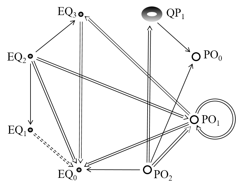
Figure 14: Topology of connections. Double lines represent multiple distinct connections. Solid (dashed) lines represent short (long) connections.

	ECS-∞	ECS∞	d	$d_{u}^{-\infty}$	$k_{s}^{\infty}$
DC1, DC2	EQ2	EQ0	2	2	0
DC3	EQ2	EQ1	1	2	1
DC4, DC5	EQ1	EQ0	1	1	0
DC6–DC9	EQ2	PO1	1	2	1
DC10	EQ2	EQ3	1	2	1
DC11, DC12	EQ3	EQ0	1	1	0
DC13, DC14, DC17	PO1	EQ0	2	2	0
DC15, DC18	PO1	PO1	1	2	1
DC16, DC19	PO1	EQ3	1	2	1
DC20	PO2	EQ0	2	2	0
DC21, DC22	PO2	PO1	1	2	1
DC23	PO2	PO0	2	2	0
DC24, DC25	PO2	QP1	1	2	1
DC26	QP1	PO0	3	3	0

Table 2: Dynamical connections computed at $Re=22.05$.

III.6 Transient Turbulence

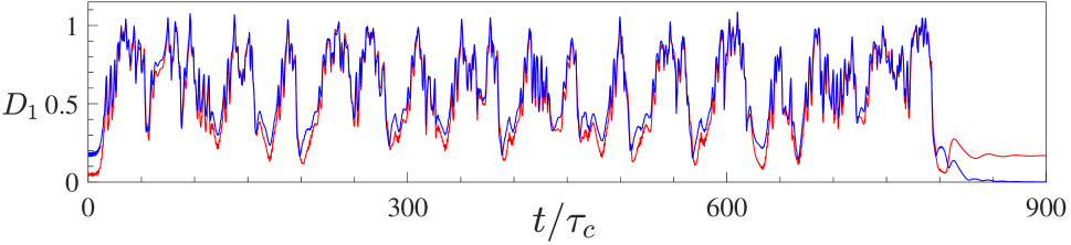
Figure 15: Instantaneous distances from a long transient turbulent trajectory to PO₁ ($D_{1}$, red) and EQ₀ ($D_{0}$, blue). Repeated close passes to PO₁ suggest that the homoclinic tangle between the stable and unstable manifolds of PO₁ underpins transient turbulence in symmetric subspace. Vanishing of $D_{0}$ implies convergence to EQ₀.

As we discussed previously, turbulence in the symmetry subspace $\mathcal{S}$ is transient, with most initial conditions eventually “relaminarizing” by converging to the stable equilibrium EQ₀. While some states relaminarize relatively quickly, others stay turbulent for a significant interval of time. It is natural to ask what geometric structures are responsible for maintaining turbulent flow and for relaminarization. Our results show that the periodic orbit PO₁ plays a key role in both processes. As we have demonstrated, PO₁ possesses (at least) two distinct homoclinic connections (DC₁₅, DC₁₈). The presence of homoclinic connections, which lie at the intersection of the stable and unstable manifold of PO₁, suggests that these manifolds intersect and form a homoclinic tangle. The tangle explains the fractal nature of the minimal state space speed shown in Fig. 10 which results from stretching and folding of the unstable manifold. More importantly, it implies the presence of a chaotic set (a chaotic repeller in our case) anchored by PO₁ as well as the presence of arbitrarily long periodic orbits that visit the neighborhood of PO₁ Smale (1967). These are precisely the ingredients required for transient turbulence.

To show that it is indeed the homoclinic tangle associated with PO₁ that underlies transient turbulence in our system, we computed the distance $D_{1}$ ($D_{0}$) from PO₁ (EQ₀) to a particular long turbulent trajectory. As Fig. 15 demonstrates, the trajectory returns to the vicinity of PO₁ many times before finally relaminarizing i.e., converging to EQ₀ ($D_{0}\rightarrow 0$). Furthermore, just before relaminarization, this trajectory comes very close to PO₁, which suggests PO₁ plays an important role in this process. It should be pointed out that not all trajectories approach PO₁ closely just before relaminarization. For instance, some trajectories pass through the neighborhood of EQ₃ instead, as Fig. 11 illustrates. Both PO₁ and EQ₃ have stable manifolds with co-dimension one; states on one side of these manifolds relaminarize almost immediately and those on the other side exhibit transient turbulence. Hence, these two stable manifolds form portions of a local boundary between “laminar” and “turbulent” flows. This analogy, however, is not perfect since the chaotic set underlying the turbulent transient is not an attractor.

It should be mentioned that non-uniqueness of edge states lying on a “laminar-turbulent” boundary has been previously reported for other turbulent flows as well. For instance, Kerswell Kerswell and Tutty (2007) and Duguet et al.aDuguet et al. (2008b) have identified several edge states corresponding to different traveling wave solutions in a short periodic pipe. Our results provide further evidence that not only can multiple edge states coexist, they can be of different types (e.g., an EQ and a PO, in our case).

The relationship between transient turbulence and chaotic repellers has been suggested previously, mainly based on indirect evidence – the power law decay of the relaminarization times characterizing a memoryless process Hof et al. (2006); Eckhardt et al. (2007); Schneider et al. (2010); Borrero-Echeverry et al. (2010). Direct evidence, such as the presence of homoclinic tangles van Veen and Kawahara (2011); Burak Budanur et al. (2018) or a period-doubling cascade Kreilos and Eckhardt (2012), is more recent. Moreover, while the dynamics and stability in systems with heteroclinic cycles have been explored previously Kirk and Silber (1994); Krupa and Melbourne (1995), there is currently very little understanding of dynamics in the presence of both heteroclinic and homoclinic connections. Due to the relative simplicity of the numerical model and ease of experimental access, the system considered here is particularly attractive for studying the relation between transient dynamics, relaminarization, and the structure of connections.

IV Summary and Conclusions

Several recent studies on a dynamical description of fluid turbulence focused on ECSs and how they shape the state space geometry in their neighborhoods. However, complete understanding of turbulence requires a global picture which explains how the flow moves between neighborhoods of ECSs. Such a picture can be considered as a coarse description of the dynamics, in the spirit of symbolic dynamics, analogous to a route network where ECSs serve as nodes and dynamical (homo/heteroclinic) connections as links connecting the nodes. This study describes the first rigorous attempt to construct such a network for a turbulent fluid flow. We identified eight nodes and several tens of connections between them, far more than any study to date. Moreover, while most previous studies computed connections between ECSs of the same type (primarily EQs), we have identified connections between three different types of ECSs: EQ, PO, and QPO. Indeed, this is the first study to compute connections involving QPOs. We have also demonstrated, for the first time, the existence of higher (two/three) dimensional connections between ECSs, i.e., continua of trajectories from one ECS to another.

Despite the limited attention they have received, dynamical connections can play a very important role in turbulent evolution Gibson et al. (2008). For instance, dynamically dominant ECSs in the Kolmogorov-like flow are equilibria Suri et al. (2018). Being fixed points in the state space, EQs cannot guide turbulent trajectories in their neighborhoods in the same way POs or QPOs do. Therefore, connections between EQs (as well as other types of ECSs) become the dynamically dominant solutions that guide turbulent trajectories, shaping their evolution locally. Even in systems where the dominant solutions are POs or QPOs, ECSs constrain the dynamics only locally in state space and over short intervals of time. The network of connections, on the other hand, constrains the dynamics globally in state space and over arbitrarily long time intervals.

Identifying the connection network has potential applications such as forecasting Suri et al. (2017) and control of turbulent flows Hof et al. (2010); Kühnen et al. (2018). Even though quantitative prediction has a time horizon set by the leading Lyapunov exponents that characterize the sensitivity to initial conditions, qualitative predictions do not have this limitation. In principle, prediction of extreme events can be made based on the connectivity of different ECSs. Identifying the connection network can also facilitate “low-energy” control of turbulent flows, where small perturbations to the flow result in its subsequent (natural) evolution towards a particular ECS or region of state space with desired behavior Pringle et al. (2012). Connections can also provide new insight into laminar-turbulent transition in wall-bounded 3D shear flows Budanur and Hof (2017); Burak Budanur et al. (2018).

Lastly, we point out that constraining the dynamics to a symmetry invariant subspace lowered the dimensionality of unstable manifolds and dramatically simplified the procedure of computing connections between ECSs. Whether these connections are dynamically relevant in the full state space requires further exploration. Currently, we are lacking robust numerical methods for computing connections between ECSs with more than one or two unstable directions. Some approaches, such as adjoint looping have shown promise Farano et al. (2018), but whether they present a viable option for computing connections between different types of ECS remains an open problem.

Appendix A State Space Projections

In this appendix we briefly describe the procedure used to project the state space onto a low-dimensional subspace spanned by the eigenvectors (Floquet vectors) ${\,\bf\hat{e}}_{i}$ of an equilibrium (periodic orbit). Each trajectory ${\bf u}(t)$ is expressed as a linear combination of the vectors ${{\,\bf\hat{e}}_{i}}$ as follows:

$${\bf u}(t)={\bf u}_{ecs}+\sum\limits_{i}a_{i}(t){\,\bf\hat{e}}_{i}.$$ (10)

Here, ${\bf u}_{ecs}$ corresponds to an equilibrium (e.g., EQ₀) or a point on a periodic orbit (e.g., PO₁). The coefficients $a_{i}(t)$ are computed using the scalar product

$$a_{i}(t)={\,\bf\hat{e}}_{i}^{\dagger}\cdot({\bf u}(t)-{\bf u}_{ecs}),$$ (11)

where ${\,\bf\hat{e}}_{i}^{\dagger}$ is the adjoint eigenvector (Floquet vector) such that ${\,\bf\hat{e}}_{i}^{\dagger}\cdot{\,\bf\hat{e}}_{j}=\delta_{ij}$ (Kronecker delta). Typically, the vectors ${\,\bf\hat{e}}_{i}$ are not orthonormal (${\,\bf\hat{e}}_{i}\cdot{\,\bf\hat{e}}_{j}\neq\delta_{ij}$). Hence, we construct orthonormalized vectors ${\,\bf\hat{e}}_{j}^{\prime}$ such that

$${\,\bf\hat{e}}_{i}=\sum\limits_{j}T_{ij}{\,\bf\hat{e}}_{j}^{\prime},$$ (12)

where, the matrix elements $T_{ij}={\,\bf\hat{e}}_{i}\cdot{\,\bf\hat{e}}_{j}^{\prime}$ can be computed using the orthonormality condition ${\,\bf\hat{e}}_{i}^{\prime}\cdot{\,\bf\hat{e}}_{j}^{\prime}=\delta_{ij}$. The normalized components

$$c_{j}=\sum\limits_{i}a_{i}T_{ij}/D_{c}$$ (13)

along vectors ${\,\bf\hat{e}}_{i}^{\prime}$ are plotted to generate state space projections. Here, $D_{c}$ is the empirically estimated largest separation between two states on a long turbulent trajectory (cf. Sect. III.1).

Appendix B Recurrence analysis

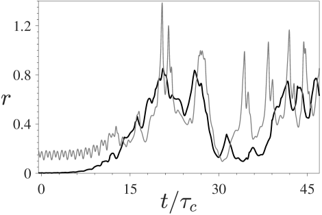
(a)

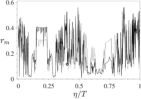
(b)

Figure 16: Recurrence analysis to detect signatures of both EQs and POs (a) Recurrence (black curve) and speed (gray curve) plots for a trajectory that originates at PO₁ and visits the neighborhoods of EQ₀ ($t/\tau_{c}=30$) and PO₂ ($t/\tau_{c}\in[33,40]$). (b) Minimum recurrence $r_{m}$ (black curve) and minimum speed $s_{m}$ (gray curve) for each trajectory ${\bf u}^{-}({\eta,t})$ from PO₁. Trajectories with $r_{m}\ll 1$ ($s_{m}\ll 1$) correspond to dynamical connections from PO₁ to EQs/POs (EQs). $s_{m}$ was scaled such that $r_{m}$, $s_{m}$ have the same mean. Black circle indicates $r_{m}$ for the trajectory shown in panel (a).

In sections III.1-III.4 we identified close passes to EQs by computing state space speed $s(t)$ along turbulent trajectories (cf. Fig. 4). However, $s(t)$ is not zero (or constant) for POs, so detecting close passes to POs requires visual inspection of speed plots to find intervals of oscillatory behavior. To address this shortcoming, we tested recurrence analysis Eckmann et al. (1987) in a form similar to that discussed in Duguet et al.aDuguet et al. (2008a). For each trajectory ${\bf u}(t)$ we computed the normalized recurrence function

$$r(t)=\min\limits_{\tau\in[\tau_{l},\tau_{h}]}\frac{\|{\bf u}(t)-{\bf u}(t+\tau)\|}{D_{c}},$$ (14)

where $0<\tau_{l}<\tau_{h}$ are appropriately chosen constants. Low values of $r$ indicate that the flow field at an instant $t$ nearly recurs during a later interval $[t+\tau_{l},t+\tau_{h}]$. Unlike state space speed, $r(t)=0$ for ${\bf u}(t)$ representing both EQs and POs. In the former case $\tau_{l}$ and $\tau_{h}$ are arbitrary, while in the latter case the period $T$ of the orbit should lie inside the interval $[\tau_{l},\tau_{h}]$.

Since a turbulent trajectory shadowing an ECS mimics its spatiotemporal behavior, intervals where $r(t)\ll 1$ correspond to the trajectory visiting neighborhoods of EQs or POs. To identify such visits, however, we should restrict how near (or far) into the future we search for recurrence. Choosing $\tau_{l}$ far smaller than the correlation time $\tau_{c}$ leads to spurious self-recurrence since ${\bf u}(t)$ and ${\bf u}(t+\tau)$ do not differ appreciably; the extreme case being $r(t)=0$ when $\tau_{l}=0$. The upper bound $\tau_{h}$ restricts the search to short periodic orbits (which tend to be dynamically relevant Cvitanović and Gibson (2010)) with period $T<\tau_{h}$. Besides, it also limits the overhead associated with computing $r(t)$. In our analysis we chose $\tau_{l}=\tau_{c}$ and $\tau_{h}=5\tau_{c}$.

Fig. 16(a) shows recurrence (black curve) and speed (gray curve) plots for a turbulent trajectory ${\bf u}(t)$ that originates at PO₁. Initially, ${\bf u}(t)$ shadows PO₁ and consequently $s(t)$ displays steady oscillations about a finite value; in contrast, $r(t)$ almost vanishes. After a brief turbulent excursion characterized by $r$ increasing to $O(1)$, ${\bf u}(t)$ visits the neighborhoods of EQ₀ at $t/\tau_{c}\approx 30$ and PO₂ for $33\lesssim t/\tau_{c}\lesssim 40$. Both these close passes correspond to $r$ decreasing to well below unity. Hence, to identify signatures of dynamical connections from PO₁ to both EQs and POs, we computed $r(\eta,t)$ for each ${\bf u}^{-}(\eta,t)$ in the unstable manifold of PO₁ (cf. Sect. III.2). We then computed $r_{m}(\eta)=\min_{t}r(\eta,t)$ for $t>15\tau_{c}$, i.e., after each trajectory initially leaves the neighborhood of PO₁. The results are shown in Fig. 16(b) which compares $r_{m}(\eta)$ (black curve) with $s_{m}(\eta)$ (gray curve) for each trajectory ${\bf u}^{-}(\eta,t)$. Clearly, the prominent minima of the two metrics align, which suggests that recurrence-based analysis is capable of successfully identifying signatures of close passes to both EQs and POs. However, it is a slightly more expensive method to identify connections, compared with the minimal state space speed.

References

- Kerswell (2005) R. R. Kerswell, Nonlinearity 18, R17 (2005).
- Kawahara et al. (2012) G. Kawahara, M. Uhlmann, and L. van Veen, Annu. Rev. Fluid Mech. 44, 203 (2012).
- Hof et al. (2004) B. Hof, C. W. H. van Doorne, J. Westerweel, F. T. M. Nieuwstadt, H. Faisst, B. Eckhardt, H. Wedin, R. R. Kerswell, and F. Waleffe, Science 305, 1594 (2004).
- de Lozar et al. (2012) A. de Lozar, F. Mellibovsky, M. Avila, and B. Hof, Phys. Rev. Lett. 108, 214502 (2012).
- Suri et al. (2017) B. Suri, J. Tithof, R. O. Grigoriev, and M. F. Schatz, Phys. Rev. Lett. 118, 114501 (2017).
- Hopf (1948) E. Hopf, Commun. Pur. Appl. Math. 1, 303 (1948).
- Gibson et al. (2008) J. F. Gibson, J. Halcrow, and P. Cvitanović, J. Fluid Mech. 611, 107 (2008).
- Note (1) See supplementary material at [xxx] for (a) Videos showcasing side-by-side evolution in state space and physical space for connections DC1, DC3, DC6, DC10, DC11, DC13, DC15, DC20, and DC23 (b) State space speed analysis of trajectories in the unstable manifold of PO2.
- Duguet et al. (2008a) Y. Duguet, A. P. Willis, and R. R. Kerswell, J. Fluid Mech. 613, 255 (2008a).
- Viswanath and Cvitanovic (2009) D. Viswanath and P. Cvitanovic, J. Fluid Mech. 627, 215–233 (2009).
- Suri et al. (2018) B. Suri, J. Tithof, R. O. Grigoriev, and M. F. Schatz, Phys. Rev. E 98, 023105 (2018).
- Halcrow et al. (2009) J. Halcrow, J. F. Gibson, P. Cvitanović, and D. Viswanath, J. Fluid Mech. 621, 365 (2009).
- Farano et al. (2018) M. Farano, S. Cherubini, J.-C. Robinet, P. De Palma, and T. M. Schneider, Journal of Fluid Mechanics 858, R3 (2018).
- Kerswell and Tutty (2007) R. R. Kerswell and O. R. Tutty, J. Fluid Mech. 584, 69–102 (2007).
- Kawahara and Kida (2001) G. Kawahara and S. Kida, J. Fluid Mech. 449, 291 (2001).
- Kawahara (2005) G. Kawahara, Phys. Fluids 17, 041702 (2005).
- Viswanath (2007) D. Viswanath, J. Fluid Mech. 580, 339 (2007).
- Gibson et al. (2009) J. F. Gibson, J. Halcrow, and P. Cvitanović, J. Fluid Mech. 638, 243 (2009).
- Faisst and Eckhardt (2003) H. Faisst and B. Eckhardt, Phys. Rev. Lett. 91, 224502 (2003).
- Wedin and Kerswell (2004) H. Wedin and R. Kerswell, J. Fluid Mech. 508, 333 (2004).
- Pringle and Kerswell (2007) C. C. T. Pringle and R. R. Kerswell, Phys. Rev. Lett. 99, 074502 (2007).
- Waleffe (2001) F. Waleffe, J. Fluid Mech. 435, 93 (2001).
- Itano and Toh (2001) T. Itano and S. Toh, J. Phys. Soc. Jpn. 70, 703 (2001).
- Toh and Itano (2003) S. Toh and T. Itano, J. Fluid Mech. 481, 67–76 (2003).
- Kim et al. (1987) J. Kim, P. Moin, and R. Moser, Journal of Fluid Mechanics 177, 133 (1987).
- Hamilton et al. (1995) J. M. Hamilton, J. Kim, and F. Waleffe, J. Fluid Mech. 287 (1995).
- Wang et al. (2007) J. Wang, J. Gibson, and F. Waleffe, Phys. Rev. Lett. 98, 204501 (2007).
- Duguet et al. (2008b) Y. Duguet, C. C. T. Pringle, and R. R. Kerswell, Phys. Fluids 20, 114102 (2008b).
- Cvitanović and Gibson (2010) P. Cvitanović and J. F. Gibson, Phys. Scripta 2010, 014007 (2010).
- Budanur et al. (2017) N. B. Budanur, K. Y. Short, M. Farazmand, A. P. Willis, and P. Cvitanović, J. Fluid Mech. 833, 274–301 (2017).
- Lemoult et al. (2014) G. Lemoult, K. Gumowski, J.-L. Aider, and J. E. Wesfreid, Eur. Phys. J. E 37, 1 (2014).
- Budanur and Hof (2017) N. B. Budanur and B. Hof, Journal of Fluid Mechanics 827, R1 (2017).
- Smale (1967) S. Smale, Bulletin of the American mathematical Society 73, 747 (1967).
- van Veen and Kawahara (2011) L. van Veen and G. Kawahara, Phys. Rev. Lett. 107, 114501 (2011).
- van Veen et al. (2011) L. van Veen, G. Kawahara, and M. Atsushi, SIAM J. Sci. Comput. 33, 25 (2011).
- Kline et al. (1967) S. Kline, W. Reynolds, F. Schraub, and P. Runstadler, J. Fluid Mech. 30, 741 (1967).
- Riols et al. (2013) A. Riols, F. Rincon, C. Cossu, G. Lesur, P.-Y. Longaretti, G. I. Ogilvie, and J. Herault, Journal of Fluid Mechanics 731, 1 (2013).
- Pershin et al. (2019) A. Pershin, C. Beaume, and S. M. Tobias, Journal of Fluid Mechanics 867, 414 (2019).
- Burak Budanur et al. (2018) N. Burak Budanur, A. Shaurya Dogra, and B. Hof, arXiv e-prints , arXiv:1810.02211 (2018), arXiv:1810.02211 [physics.flu-dyn] .
- Bondarenko et al. (1979) N. F. Bondarenko, M. Z. Gak, and F. V. Dolzhanskiy, Izv. Akad. Nauk SSSR, Fiz. Atmos. Okeana 15, 711 (1979).
- Suri et al. (2014) B. Suri, J. Tithof, R. Mitchell, R. O. Grigoriev, and M. F. Schatz, Phys. Fluids 26, 053601 (2014).
- Chandler and Kerswell (2013) G. J. Chandler and R. R. Kerswell, J. Fluid Mech. 722, 554 (2013).
- Lucas and Kerswell (2014) D. Lucas and R. R. Kerswell, J. Fluid Mech. 750, 518 (2014).
- Farazmand (2016) M. Farazmand, J. Fluid Mech. 795, 278–312 (2016).
- Cvitanović (1988) P. Cvitanović, Phys. Rev. Lett. 61, 2729 (1988).
- Tithof et al. (2017) J. Tithof, B. Suri, R. K. Pallantla, R. O. Grigoriev, and M. F. Schatz, J. Fluid Mech. 828, 837 (2017).
- Armfield and Street (1999) S. Armfield and R. Street, J. Comput. Phys. 153, 660 (1999).
- Suri (2017) B. Suri, Quasi-Two-Dimensional Kolmogorov flow: Bifurcations and Exact Coherent Structures, Ph.D. thesis, Georgia Institute of Technology (2017).
- Farmer et al. (1983) J. Farmer, E. Ott, and J. A. Yorke, Physica D: Nonlinear Phenomena 7, 153 (1983).
- Neelavara et al. (2017) S. A. Neelavara, Y. Duguet, and F. Lusseyran, Fluid Dynamics Research 49, 035511 (2017).
- Saad and Schultz (1986) Y. Saad and M. H. Schultz, SIAM J. Sci. Stat. Comp. 7, 856 (1986).
- Kelley (2003) C. Kelley, Solving Nonlinear Equations with Newton’s Method (SIAM, 2003).
- Mitchell (2013) R. Mitchell, Transition to turbulence and mixing in a quasi-two-dimensional Lorentz force-driven Kolmogorov flow, Ph.D. thesis, Georgia Institute of Technology (2013).
- Avila et al. (2013) M. Avila, F. Mellibovsky, N. Roland, and B. Hof, Phys. Rev. Lett. 110, 224502 (2013).
- Hof et al. (2006) B. Hof, J. Westerweel, T. M. Schneider, and B. Eckhardt, Nature 443, 59 (2006).
- Eckhardt et al. (2007) B. Eckhardt, H. Faisst, A. Schmiegel, and T. M. Schneider, Philosophical Transactions of the Royal Society A: Mathematical, Physical and Engineering Sciences 366, 1297 (2007).
- Schneider et al. (2010) T. M. Schneider, F. De Lillo, J. Buehrle, B. Eckhardt, T. Dörnemann, K. Dörnemann, and B. Freisleben, Physical review E 81, 015301 (2010).
- Borrero-Echeverry et al. (2010) D. Borrero-Echeverry, M. F. Schatz, and R. Tagg, Physical Review E 81, 025301 (2010).
- Kreilos and Eckhardt (2012) T. Kreilos and B. Eckhardt, Chaos: An Interdisciplinary Journal of Nonlinear Science 22, 047505 (2012).
- Kirk and Silber (1994) V. Kirk and M. Silber, Nonlinearity 7, 1605 (1994).
- Krupa and Melbourne (1995) M. Krupa and I. Melbourne, Ergodic Theory and Dynamical Systems 15, 121 (1995).
- Hof et al. (2010) B. Hof, A. de Lozar, M. Avila, X. Tu, and T. M. Schneider, Science 327, 1491 (2010).
- Kühnen et al. (2018) J. Kühnen, B. Song, D. Scarselli, N. B. Budanur, M. Riedl, A. P. Willis, M. Avila, and B. Hof, Nature Physics 14, 386 (2018).
- Pringle et al. (2012) C. C. Pringle, A. P. Willis, and R. R. Kerswell, Journal of Fluid Mechanics 702, 415 (2012).
- Eckmann et al. (1987) J.-P. Eckmann, S. O. Kamphorst, and D. Ruelle, Europhys. Lett. 4, 973 (1987).