Neutral and charged pion properties under strong magnetic fields in the NJL model

Abstract

In the framework of the Nambu–Jona-Lasino (NJL) model, we study the effect of an intense external uniform magnetic field on neutral and charged pion masses and decay form factors. In particular, the treatment of charged pions is carried out on the basis of the Ritus eigenfunction approach to magnetized relativistic systems. Our analysis shows that in the presence of the magnetic field three and four nonvanishing pion-to-vacuum hadronic form factors can be obtained for the case of the neutral and charged pions, respectively. As expected, it is seen that for nonzero magnetic field the $\pi^{0}$ meson can still be treated as a pseudo Nambu-Goldstone boson, and consequently the corresponding form factors are shown to satisfy various chiral relations. For definite parametrizations of the model, numerical results for $\pi^{0}$ and $\pi^{\pm}$ masses and decay constants are obtained and compared with previous calculations given in the literature.

I Introduction

In recent years a significant effort has been devoted to the study of the properties of strongly interacting matter under the influence of strong magnetic fields (see e.g. Kharzeev:2012ph ; Andersen:2014xxa ; Miransky:2015ava and references therein). This is mostly motivated by the realization that large magnetic fields might play an important role in the physics of the early Universe Grasso:2000wj , in the analysis of high energy noncentral heavy ion collisions HIC , and in the description of physical systems such as magnetars duncan . From the theoretical point of view, addressing this subject requires one to deal with quantum chromodynamics (QCD) in nonperturbative regimes. Therefore, existing analyses are based either in the predictions of effective models or in the results obtained through lattice QCD (LQCD) calculations. In this work we focus on the effect of an intense external magnetic field on $\pi$ meson properties. This issue has been studied in the last years following various theoretical approaches for low energy QCD, such as Nambu-Jona-Lasinio (NJL)-like models Fayazbakhsh:2013cha ; Fayazbakhsh:2012vr ; Avancini:2015ady ; Zhang:2016qrl ; Avancini:2016fgq ; Mao:2017wmq ; GomezDumm:2017jij ; Wang:2017vtn ; Liu:2018zag ; Coppola:2018vkw ; Mao:2018dqe ; Avancini:2018svs , quark-meson models Kamikado:2013pya ; Ayala:2018zat , chiral perturbation theory (ChPT) Andersen:2012zc ; Agasian:2001ym ; Colucci:2013zoa , path integral Hamiltonians Orlovsky:2013wjd ; Andreichikov:2016ayj , effective chiral confinement Lagrangian approach (ECCL) Simonov:2015xta ; Andreichikov:2018wrc , QCD sum rules (SRQCD) Dominguez:2018njv , etc. In addition, results for the light meson spectrum in the presence of background magnetic fields have been recently obtained from LQCD calculations Bali:2011qj ; Hidaka:2012mz ; Luschevskaya:2014lga ; Bali:2015vua ; Bali:2017ian .

In the framework of the NJL model, mesons are usually described as quantum fluctuations in the random phase approximation (RPA) Vogl:1991qt ; Klevansky:1992qe ; Hatsuda:1994pi , i.e., they are introduced via the summation of an infinite number of quark loops. In the presence of a magnetic field $\vec{B}$, the calculation of these loops requires some care due to the appearance of Schwinger phases Schwinger:1951nm associated with quark propagators. For the neutral pion these phases cancel out, and as a consequence the usual momentum basis can be used to diagonalize the corresponding polarization function Fayazbakhsh:2013cha ; Fayazbakhsh:2012vr ; Avancini:2015ady ; Avancini:2016fgq ; Mao:2017wmq . On the other hand, for charged pions the Schwinger phases do not cancel, leading to a breakdown of translational invariance that prevents one from proceeding as in the $\pi^{0}$ case. In this situation, some existing calculations Zhang:2016qrl ; Liu:2018zag just neglect Schwinger phases, considering only the translational invariant part of the quark propagators. Recently Coppola:2018vkw , a method was proposed in order to fully take into account the translational-breaking effects introduced by the Schwinger phases in the calculation of charged meson masses within the RPA. This method, based on the Ritus eigenfunction approach Ritus:1978cj to magnetized relativistic systems, allows one to diagonalize the charged pion polarization function for the obtention of the corresponding meson masses. In addition, the analysis in Ref. Coppola:2018vkw considers a regularization procedure in which only the vacuum contributions to different quantities at zero external magnetic field are regularized. This scheme, that goes under the name of “magnetic field independent regularization” (MFIR), has been shown to provide more reliable predictions in comparison with other regularization methods often used in the literature Avancini:2019wed .

The scope of the present work is to consider the approach introduced in Ref. Coppola:2018vkw for the study of pion masses, extending the calculations to other properties of neutral and charged pions. In particular, we concentrate in the analysis of the form factors associated with the pion-to-vacuum matrix elements of the vector and axial vector hadronic currents. For the case of the $\pi^{0}$, some works Fayazbakhsh:2013cha ; Agasian:2001ym ; Andersen:2012zc ; Fayazbakhsh:2012vr ; Avancini:2015ady ; Zhang:2016qrl ; Avancini:2016fgq ; Mao:2017wmq ; Kamikado:2013pya ; GomezDumm:2017jij ; Simonov:2015xta ; Andreichikov:2018wrc have already considered the $B$ dependence of the decay constant $f_{\pi^{0}}^{(A1)}$, which corresponds to the time component of the axial vector current matrix element. For charged pions, the effect of the magnetic field has been analyzed in the context of ChPT Andersen:2012zc , ECCL approach Simonov:2015xta , SRQCD Dominguez:2018njv and, quite recently, through LQCD calculations Bali:2018sey . An interesting observation made in Ref. Fayazbakhsh:2013cha states that, due to the explicit breaking of rotational invariance caused by the magnetic field, one can define two different decay constants. One of them is associated with the direction parallel to $\vec{B}$ (and to the time direction) and the other with the spatial directions perpendicular to $\vec{B}$. A further relevant statement has been pointed out in Ref. Bali:2018sey . In that work it is noted that the presence of the background magnetic field opens the possibility of a nonzero charged pion-to-vacuum transition via the vector piece of the electroweak current. This implies the existence of a further decay constant associated with the pion-to-vacuum matrix element of the vector current. Furthermore, in a recent work Coppola:2018ygv we have shown that (i) the pion-to-vacuum matrix element of the vector current can be nonvanishing even in the case of the neutral pion, and (ii) for the charged pions there are in general not two but three nonvanishing axial decay constants. The aim of the present paper is to study the behavior of all these form factors as functions of the magnetic field in the context of the NJL model within the MFIR regularization scheme.

This work is organized as follows. In Sec. II we introduce the theoretical formalism used to obtain the different quantities we are interested in. Chiral limit relations are addressed in Sec. III. Then, in Sec. IV we present and discuss our numerical results, while in Sec. V we provide a summary of our work, together with our main conclusions. We also include Appendixes A and B to quote some technical details of our calculations.

II Theoretical Formalism

II.1 Mean field properties and pion masses

We start by considering the Euclidean Lagrangian density for the NJL two-flavor model in the presence of an electromagnetic field. One has

$${\cal L}\ =\ \bar{\psi}\left(-i\,\hbox to0.0pt{/\hss}\!D+m_{0}\right)\psi-G\left[(\bar{\psi}\,\psi)^{2}+(\bar{\psi}\,i\gamma_{5}\vec{\tau}\,\psi)\right]\ ,\qquad\psi=\left(\begin{array}[]{c}\psi_{u}\\ \psi_{d}\end{array}\right)\ ,$$ (1)

where $\tau_{i}$ are the Pauli matrices and $m_{0}$ is the current quark mass, which is assumed to be equal for $u$ and $d$ quarks. The interaction between the fermions and the electromagnetic field ${\cal A}_{\mu}$ is driven by the covariant derivative

$$D_{\mu}\,=\,\partial_{\mu}-i\,\hat{Q}\mathcal{A}_{\mu}\ ,$$ (2)

where $\hat{Q}=\mbox{diag}(q_{u},q_{d})$, with $q_{u}=2e/3$ and $q_{d}=-e/3$, $e$ being the proton electric charge. We will consider the particular case of an homogenous stationary magnetic field $\vec{B}$ along the positive 3-axis. Let us choose the Landau gauge, in which $\mathcal{A}_{4}=0$, $\vec{\mathcal{A}}=(0,Bx_{1},0)$.

Since we are interested in studying meson properties, it is convenient to bosonize the fermionic theory, introducing scalar $\sigma(x)$ and pseudoscalar $\vec{\pi}(x)$ fields and integrating out the fermion fields. The bosonized Euclidean action can be written as Klevansky:1992qe

$$S_{\mathrm{bos}}\,=\,-\log\det\mathcal{D}+\frac{1}{4G}\int d^{4}x\ \Big{[}\sigma(x)\sigma(x)+\vec{\pi}(x)\cdot\vec{\pi}(x)\Big{]}\ ,$$ (3)

with

$$\mathcal{D}_{x,x^{\prime}}\,=\,\delta^{(4)}(x-x^{\prime})\,\left[-i\,\hbox to0.0pt{/\hss}\!D+m_{0}+\sigma(x)+i\,\gamma_{5}\,\vec{\tau}\cdot\vec{\pi}(x)\right]\ ,$$ (4)

where a direct product to an identity matrix in color space is understood.

We proceed by expanding the bosonized action in powers of the fluctuations $\delta\sigma(x)$ and $\delta\pi_{i}(x)$ around the corresponding mean field (MF) values. As usual, we assume that the field $\sigma(x)$ has a nontrivial translational invariant mean field value $\bar{\sigma}$, while the vacuum expectation values of pseudoscalar fields are zero. Thus we write

$$\mathcal{D}_{x,x^{\prime}}\ =\ \mathcal{D}^{\mbox{\tiny MF}}_{x,x^{\prime}}+\delta\mathcal{D}_{x,x^{\prime}}\ .$$ (5)

The MF piece is flavor diagonal. It can be written as

$$\mathcal{D}^{\mbox{\tiny MF}}_{x,x^{\prime}}\ =\ {\rm diag}\big{(}\mathcal{D}^{{\mbox{\tiny MF}},u}_{x,x^{\prime}}\,,\,\mathcal{D}^{{\mbox{\tiny MF}},d}_{x,x^{\prime}}\big{)}\ ,$$ (6)

where

$$\mathcal{D}^{{\mbox{\tiny MF}},f}_{x,x^{\prime}}\ =\ \delta^{(4)}(x-x^{\prime})\left(-i\hbox to0.0pt{/\hss}\partial-q_{f}\,B\,x_{1}\,\gamma_{2}+m_{0}+\bar{\sigma}\right).$$ (7)

On the other hand, the second term on the right-hand-side of Eq. (5) is given by

$$\delta D_{x,x^{\prime}}\ =\ \delta^{(4)}(x-x^{\prime})\,\begin{pmatrix}\delta\sigma(x)+i\gamma_{5}\delta\pi_{0}(x)&\sqrt{2}i\gamma_{5}\,\delta\pi^{+}(x)\\ \sqrt{2}i\gamma_{5}\,\delta\pi^{-}(x)&\delta\sigma(x)-i\gamma_{5}\delta\pi_{0}(x)\end{pmatrix}\ ,$$ (8)

where $\pi^{\pm}=\left(\pi_{1}\mp i\pi_{2}\right)/\sqrt{2}$. Replacing in the bosonized effective action and expanding in powers of the meson fluctuations around the MF values, we get

$$S_{\mathrm{bos}}\ =\ S^{\mbox{\tiny MF}}_{\mathrm{bos}}\,+\,S^{\,\mbox{\tiny quad}}_{\mathrm{bos}}\,+\,\dots$$ (9)

Here, the mean field action per unit volume reads

$$\frac{S^{\mbox{\tiny MF}}_{\mathrm{bos}}}{V^{(4)}}\ =\ \frac{\bar{\sigma}^{2}}{4G}-\frac{N_{c}}{V^{(4)}}\sum_{f=u,d}\int d^{4}x\,d^{4}x^{\prime}\ {\rm tr}_{D}\,\ln\left(\mathcal{S}^{\mbox{\tiny MF},f}_{x,x^{\prime}}\right)^{-1}\ ,$$ (10)

where ${\rm tr}_{D}$ stands for the trace in Dirac space. The quadratic contribution is given by

$$S^{\,\mbox{\tiny quad}}_{\mathrm{bos}}\ =\ \dfrac{1}{2}\sum_{M=\sigma,\pi^{0},\pi^{\pm}}\int d^{4}x\,d^{4}x^{\prime}\ \delta M(x)^{\ast}\left[\frac{1}{2G}\;\delta^{(4)}(x-x^{\prime})-J_{M}(x,x^{\prime})\right]\delta M(x^{\prime})\ ,$$ (11)

where

$$J_{\pi^{0}}(x,x^{\prime}) = N_{c}\sum_{f}{\rm tr}_{D}\bigg{[}\mathcal{S}^{{\mbox{\tiny MF}},f}_{x,x^{\prime}}\ \gamma_{5}\ \mathcal{S}^{{\mbox{\tiny MF}},f}_{x^{\prime},x}\ \gamma_{5}\ \bigg{]}\ ,$$

$$J_{\pi^{-}}(x,x^{\prime}) = 2N_{c}\,{\rm tr}_{D}\bigg{[}\mathcal{S}^{{\mbox{\tiny MF}},d}_{x,x^{\prime}}\ \gamma_{5}\ \mathcal{S}^{{\mbox{\tiny MF}},u}_{x^{\prime},x}\ \gamma_{5}\ \bigg{]}\ ,$$

$$J_{\pi^{+}}(x,x^{\prime}) = 2N_{c}\,{\rm tr}_{D}\bigg{[}\mathcal{S}^{{\mbox{\tiny MF}},u}_{x,x^{\prime}}\ \gamma_{5}\ \mathcal{S}^{{\mbox{\tiny MF}},d}_{x^{\prime},x}\ \gamma_{5}\ \bigg{]}\ ,$$ (12)

while the expression for $J_{\sigma}$ is obtained from that of $J_{\pi^{0}}$ just replacing both $\gamma_{5}$ matrices for unit matrices. In these expressions we have introduced the mean field quark propagators $\mathcal{S}^{{\mbox{\tiny MF}},f}_{x,x^{\prime}}=\big{(}\mathcal{D}^{{\mbox{\tiny MF}},f}_{x,x^{\prime}}\big{)}^{-1}$. As is well known, their explicit form can be written in different ways Andersen:2014xxa ; Miransky:2015ava . For convenience we take the form in which $\mathcal{S}^{{\mbox{\tiny MF}},f}_{x,x^{\prime}}$ is given by a product of a phase factor and a translational invariant function, namely

$$S^{{\mbox{\tiny MF}},f}_{x,x^{\prime}}\ =\ e^{i\Phi_{f}(x,x^{\prime})}\,\int_{p}e^{i\,p\,(x-x^{\prime})}\,\tilde{S}_{p}^{f}\ ,$$ (13)

where $\Phi_{f}(x,x^{\prime})=q_{f}B(x_{1}+x_{1}^{\prime})(x_{2}-x_{2}^{\prime})/2$ is the so-called Schwinger phase. We have introduced here the shorthand notation

$$\int_{p}\ \equiv\ \int\dfrac{d^{4}p}{(2\pi)^{4}}\ .$$ (14)

We express $\tilde{S}_{p}^{f}$ in the Schwinger form Andersen:2014xxa ; Miransky:2015ava

$$\tilde{S}_{p}^{f}\ =\ \int_{0}^{\infty}\!d\tau\,\exp\big{[}-\tau\phi_{f}(\tau,p)\big{]}\,\Big{[}\big{(}M-p_{\parallel}\gamma_{\parallel}\big{)}\,\big{(}1+is_{f}\,\gamma_{1}\gamma_{2}\,\tanh(\tau B_{f})\big{)}-\dfrac{p_{\perp}\gamma_{\perp}}{\cosh^{2}(\tau B_{f})}\Big{]}\ ,$$ (15)

where we have used the following definitions. The “perpendicular” and “parallel” gamma matrices are collected in vectors $\gamma_{\perp}=(\gamma_{1},\gamma_{2})$ and $\gamma_{\parallel}=(\gamma_{3},\gamma_{4})$. Similarly, $p_{\perp}=(p_{1},p_{2})$ and $p_{\parallel}=(p_{3},p_{4})$. Note that in our convention $\{\gamma_{\mu},\gamma_{\nu}\}=-2\delta_{\mu\nu}$. The quark effective mass $M$ is given by $M=m_{0}+\bar{\sigma}$, and we have used the notation $s_{f}={\rm sign}(q_{f}B)$ and $B_{f}=|q_{f}B|$. Finally, we have defined

$$\phi_{f}(\tau,p)\ =\ M^{2}+p_{\parallel}^{2}+\dfrac{\tanh(\tau B_{f})}{\tau B_{f}}\;p_{\perp}^{2}\ .$$ (16)

Notice that the integral in Eq. (15) is divergent and has to be properly regularized, as we discuss below.

Replacing the above expression for the quark propagator in Eq. (10) and minimizing with respect to $M$ we obtain the gap equation

$$M\ =\ m_{0}+4GMN_{c}\,I\ ,$$ (17)

where $I$ is a divergent integral. To regularize it we use here the magnetic field independent regularization scheme Menezes:2008qt ; Allen:2015paa . That is, we subtract from $I$ the unregulated integral in the $B=0$ limit, $I_{B=0}$, and then we add it in a regulated form $I^{\rm(reg)}_{B=0}$. Thus, we have

$$I^{\rm(reg)}\ =\ I^{\rm(reg)}_{B=0}+I^{\rm(mag)}\ ,$$ (18)

where $I^{\rm(mag)}$ is a finite, magnetic field dependent contribution given by

$$I^{\rm(mag)} = \frac{1}{8\pi^{2}}\sum_{f}\int_{0}^{\infty}\!d\tau\;\frac{\exp(-\tau M^{2})}{\tau^{2}}\;\Big{[}\tau B_{f}\coth(\tau B_{f})-1\Big{]}$$ (19)

$$= \frac{M^{2}}{8\pi^{2}}\sum_{f}\left[\frac{\ln\Gamma(x_{f})}{x_{f}}-\frac{\ln 2\pi}{2x_{f}}+1-\left(1-\frac{1}{2x_{f}}\right)\ln x_{f}\right]\ ,$$

with $x_{f}=M^{2}/(2B_{f})$. On the other hand, the regulated piece $I^{\rm(reg)}_{B=0}$ does depend on the regularization prescription. Choosing the standard procedure in which one introduces a 3D momentum cutoff $\Lambda$, we get the well-known result Klevansky:1992qe

$$I^{\rm(reg)}_{B=0}\ =\ I_{1}\equiv\ \frac{1}{2\pi^{2}}\left[\Lambda\,\sqrt{\Lambda^{2}+M^{2}}+M^{2}\;\ln{\left(\frac{M}{\Lambda+\sqrt{\Lambda^{2}+M^{2}}}\right)}\right]\ .$$ (20)

For the reader’s convenience, in what remains of this subsection we review the procedure followed in Ref. Coppola:2018vkw to determine the pion masses. We start by the simpler case of the neutral pion $\pi^{0}$. In this case the contributions of Schwinger phases associated to the quark propagators cancel out. Therefore, the polarization function depends only on the difference $x-x^{\prime}$ (i.e., it is translational invariant), which leads to the conservation of $\pi^{0}$ momentum. If we take now the Fourier transform of $\pi^{0}$ fields to the momentum basis, the corresponding transform of the polarization function will be diagonal in $q,q^{\prime}$ momentum space. Thus, the $\pi^{0}$ contribution to the quadratic action in the momentum basis can be written as

$$S^{\,\mbox{\tiny quad}}_{\pi^{0}}\ =\ \dfrac{1}{2}\int_{q}\ \delta\pi^{0}(-q)\,\left[\frac{1}{2G}-J_{\pi^{0}}(q_{\perp}^{2},q_{\parallel}^{2})\right]\delta\pi^{0}(q)\ ,$$ (21)

where

$$J_{\pi^{0}}(q_{\perp}^{2},q_{\parallel}^{2})\ =\ N_{c}\sum_{f}\int_{p,v}(2\pi)^{4}\delta^{(4)}(v-q)\ {\rm tr}_{D}\,(\tilde{S}_{p^{+}}^{f}\,\gamma_{5}\,\tilde{S}_{p^{-}}^{f}\,\gamma_{5})\ ,$$ (22)

with $p^{\pm}=p\pm v/2$. Replacing Eq. (15) into Eq. (22) and using the results in Appendixes A and B one finds

$$J_{\pi^{0}}(q_{\perp}^{2},q_{\parallel}^{2}) = \dfrac{N_{c}}{4\pi^{2}}\sum_{f}\,B_{f}\int_{0}^{\infty}dz\int_{0}^{1}dy\,\exp\left\{-z\left[M^{2}+y(1-y)\,q_{\parallel}^{2}\right]\right\}\,\times$$ (23)

$$\exp\left[-\dfrac{q_{\perp}^{2}}{B_{f}}\,\gamma_{f}(y,z)\right]\bigg{\{}\Big{[}M^{2}+\dfrac{1}{z}-y(1-y)\,q_{\parallel}^{2}\Big{]}\coth(zB_{f})\,+$$

$$\dfrac{B_{f}}{\sinh^{2}(zB_{f})}\left[1-\dfrac{q_{\perp}^{2}}{B_{f}}\,\gamma_{f}(y,z)\right]\bigg{\}}\ ,$$

where

$$\gamma_{f}(y,z)\ =\ \dfrac{\sinh(zyB_{f})\sinh[(1-y)zB_{f}]}{\sinh(zB_{f})}\ .$$ (24)

As usual, here we have used the changes of variables $\tau=yz$ and $\tau^{\prime}=(1-y)z$, $\tau$ and $\tau^{\prime}$ being the integration parameters associated with the quark propagators as in Eq. (15).

As done at the MF level, we regularize the integral in Eq. (23) using the MFIR scheme. That is, we subtract the corresponding unregulated contribution in the $B=0$ limit, given by

$$J_{\pi,B=0}(q^{2})\ =\ \dfrac{N_{c}}{2\pi^{2}}\int_{0}^{\infty}\dfrac{dz}{z}\int_{0}^{1}dy\,\exp\left\{-z\left[M^{2}+y(1-y)\,q^{2}\right]\right\}\left[M^{2}+\dfrac{2}{z}-y(1-y)\,q^{2}\right]\ ,$$ (25)

and add it in a regularized form $J_{\pi,B=0}^{\rm(reg)}(q^{2})$. The regularized polarization function is then given by

$$J^{\rm(reg)}_{\pi^{0}}(q_{\perp}^{2},q_{\parallel}^{2})\ =\ J^{\rm(reg)}_{\pi,B=0}(q^{2})+J^{\rm(mag)}_{\pi^{0}}(q_{\perp}^{2},q_{\parallel}^{2})\ ,$$ (26)

where $J^{\rm(mag)}_{\pi^{0}}(q_{\perp}^{2},q_{\parallel}^{2})=J_{\pi^{0}}(q_{\perp}^{2},q_{\parallel}^{2})-J_{\pi,B=0}(q_{\perp}^{2}+q_{\parallel}^{2})$. To get $J^{\rm(reg)}_{\pi,B=0}(q^{2})$ we use the 3D momentum cutoff scheme, as in the case of the gap equation. One has in this way

$$J^{\rm(reg)}_{\pi,B=0}(q^{2})\ =\ 2N_{c}\left[I_{1}+q^{2}I_{2}(q^{2})\right]\ ,$$ (27)

where $I_{1}$ is given by Eq. (20), while

$$I_{2}(q^{2}) = \frac{1}{4\pi^{2}}\int_{0}^{1}dy\left[\frac{\Lambda}{\sqrt{\Lambda^{2}+M^{2}+y(1-y)q^{2}}}\,+\,\ln{\frac{{\sqrt{M^{2}+y(1-y)q^{2}}}}{\Lambda+\sqrt{\Lambda^{2}+M^{2}+y(1-y)q^{2}}}}\right].$$ (28)

Choosing the frame in which the $\pi^{0}$ meson is at rest, its mass can be obtained by solving the equation

$$\frac{1}{2G}-J^{\rm(reg)}_{\pi^{0}}(0,-m_{\pi^{0}}^{2})\ =\ 0\ .$$ (29)

Let us now discuss the case of charged pions. For definiteness we consider the $\pi^{-}$ meson, although a similar analysis, leading to the same expression for the $B$-dependent mass, can be carried out for the $\pi^{+}$. As in the case of the $\pi^{0}$, we start by replacing Eq. (13) in the expression of the corresponding polarization function in Eq. (12). We get

$$J_{\pi^{-}}(x,x^{\prime})\ =\ 2N_{c}\int_{p\,v}{\rm tr}_{D}(\tilde{S}_{p^{+}}^{d}\,\gamma_{5}\,\tilde{S}_{p^{-}}^{u}\,\gamma_{5})\,e^{i\Phi_{d}(x,x^{\prime})}\,e^{i\Phi_{u}(x^{\prime},x)}\,e^{iv(x-x^{\prime})}\ .$$ (30)

where once again we define $p^{\pm}=p\pm v/2$. Contrary to the $\pi^{0}$ case, here the Schwinger phases do not cancel, due to their different quark flavors. Therefore, this polarization function is not translational invariant, and consequently it will not become diagonal when transformed to the momentum basis. Therefore, we expand the charged pion field as

$$\pi^{-}(x)\ =\ \operatorname*{\mathchoice{\ooalign{$\displaystyle\sum$\cr$\displaystyle\int$\cr}}{\ooalign{\raisebox{0.14pt}{\scalebox{0.7}{$\textstyle\sum$}}\cr$\textstyle\int$\cr}}{\ooalign{\raisebox{0.2pt}{\scalebox{0.6}{$\scriptstyle\sum$}}\cr$\scriptstyle\int$\cr}}{\ooalign{\raisebox{0.2pt}{\scalebox{0.6}{$\scriptstyle\sum$}}\cr$\scriptstyle\int$\cr}}}_{\bar{q}}\ \mathbb{F}_{\bar{q}}^{-}(x)\,\pi_{\bar{q}}^{-}\ ,$$ (31)

where we have used the shorthand notation

$$\bar{q}\equiv(\breve{q},q_{4})\ ,\qquad\breve{q}\equiv(k,q_{2},q_{3})\ ,\qquad\operatorname*{\mathchoice{\ooalign{$\displaystyle\sum$\cr$\displaystyle\int$\cr}}{\ooalign{\raisebox{0.14pt}{\scalebox{0.7}{$\textstyle\sum$}}\cr$\textstyle\int$\cr}}{\ooalign{\raisebox{0.2pt}{\scalebox{0.6}{$\scriptstyle\sum$}}\cr$\scriptstyle\int$\cr}}{\ooalign{\raisebox{0.2pt}{\scalebox{0.6}{$\scriptstyle\sum$}}\cr$\scriptstyle\int$\cr}}}_{\bar{q}}\ \equiv\ \dfrac{1}{2\pi}\sum_{k=0}^{\infty}\int_{q_{2}\,q_{3}\,q_{4}}\ .$$ (32)

The functions $\mathbb{F}_{\bar{q}}^{\pm}(x)$ are given by

$$\mathbb{F}_{\bar{q}}^{\pm}(x)\ =\ N_{k}\,e^{i(q_{2}x_{2}+q_{3}x_{3}+q_{4}x_{4})}\,D_{k}(\rho_{\pm})\ ,$$ (33)

where $D_{k}(x)$ are the cylindrical parabolic functions. We have used the definitions $N_{k}=(4\pi B_{e})^{1/4}/\sqrt{k!}$ and $\rho_{\pm}=\sqrt{2B_{e}}\,x_{1}-s_{\pm}\sqrt{2/B_{e}}\,q_{2}$, where $B_{e}=|q_{\pi^{\pm}}B|=|eB|$ and $s_{\pm}=\mathrm{sign}(q_{\pi^{\pm}}B)$, with $q_{\pi^{\pm}}=\pm(q_{u}-q_{d})=\pm e$. For the $\pi^{-}$ one has

$$S^{\,\mbox{\tiny quad}}_{\pi^{-}}\ =\ \dfrac{1}{2}\operatorname*{\mathchoice{\ooalign{$\displaystyle\sum$\cr$\displaystyle\int$\cr}}{\ooalign{\raisebox{0.14pt}{\scalebox{0.7}{$\textstyle\sum$}}\cr$\textstyle\int$\cr}}{\ooalign{\raisebox{0.2pt}{\scalebox{0.6}{$\scriptstyle\sum$}}\cr$\scriptstyle\int$\cr}}{\ooalign{\raisebox{0.2pt}{\scalebox{0.6}{$\scriptstyle\sum$}}\cr$\scriptstyle\int$\cr}}}_{\bar{q}^{\prime},\bar{q}}\ (\delta\pi_{\bar{q}}^{-})^{\ast}\Big{(}\frac{1}{2G}\,\hat{\delta}_{\bar{q}\bar{q}^{\prime}}-J^{-}_{\bar{q}\bar{q}^{\prime}}\Big{)}\delta\pi_{\bar{q}^{\prime}}^{-}\ ,$$ (34)

where

$$\hat{\delta}_{\bar{q}\bar{q}^{\prime}}=(2\pi)^{4}\delta_{kk^{\prime}}\delta(q_{2}-q_{2}^{\prime})\delta(q_{3}-q_{3}^{\prime})\delta(q_{4}-q_{4}^{\prime})\ .$$ (35)

and

$$J^{-}_{\bar{q}\bar{q}^{\prime}}\ =\ 2N_{c}\int_{p\,v}\!\!{\rm tr}_{D}\left[\tilde{S}_{p^{+}}^{d}\gamma_{5}\,\tilde{S}_{p^{-}}^{u}\gamma_{5}\,\right]\int d^{4}x\,d^{4}x^{\prime}\,e^{i\Phi_{d}(x,x^{\prime})}e^{i\Phi_{u}(x^{\prime},x)}e^{iv(x-x^{\prime})}\,\mathbb{F}_{\bar{q}}^{-}(x)^{\ast}\,\mathbb{F}_{\bar{q}^{\prime}}^{-}(x^{\prime})\ .$$ (36)

Integrating over $x^{\prime}$ in Eq. (36) one obtains

$$J^{-}_{\bar{q}\bar{q}^{\prime}} = \dfrac{8\pi N_{c}}{B_{e}}\int d^{4}x\;\mathbb{F}_{\bar{q}}^{-}(x)^{\ast}\;e^{i(q^{\prime}_{2}x_{2}+q^{\prime}_{\parallel}x_{\parallel})}\int_{p\,v}\!\!(2\pi)^{2}\,\delta^{(2)}(v_{\parallel}-q_{\parallel}^{\prime})\,{\rm tr}_{D}\left[\tilde{S}_{p^{+}}^{d}\gamma_{5}\,\tilde{S}_{p^{-}}^{u}\gamma_{5}\,\right]\times$$ (37)

$$N_{k^{\prime}}\,e^{iv_{1}(x_{1}-x^{\prime}_{1})}\,D_{k^{\prime}}(\sqrt{2B_{e}}\,x_{1}^{\prime}-s_{-}\sqrt{2/B_{e}}\,q^{\prime}_{2})\Big{|}_{x_{1}^{\prime}=-x_{1}+2s_{-}(q^{\prime}_{2}-v_{2})/B_{e}}\ .$$

The integrals over the loop momenta $p$ and $v$ can be evaluated using the results in Appendixes A and B. It can be shown that the polarization function is diagonal in the chosen basis. One has

$$J^{-}_{\bar{q}\bar{q}^{\prime}}\ =\ \int d^{4}x\;\mathbb{F}_{\bar{q}}^{-}(x)^{\ast}J_{\pi^{-}}(k,\Pi^{2})\;\mathbb{F}_{\bar{q}^{\prime}}^{-}(x)\ =\ \hat{\delta}_{\bar{q}\bar{q}^{\prime}}\;J_{\pi^{-}}(k,\Pi^{2})\ ,$$ (38)

where $\Pi^{2}=(2k+1)B_{e}+q_{\parallel}^{2}$, and

$$J_{\pi^{-}}(k,\Pi^{2}) = \dfrac{N_{c}}{2\pi^{2}}\int_{0}^{\infty}\!dz\int_{0}^{1}dy\ \exp\big{[}-zM^{2}-zy(1-y)(\Pi^{2}-(2k+1)\,B_{e})\big{]}\ \times$$ (39)

$$\dfrac{\alpha_{-}^{k}}{\alpha_{+}^{k+1}}\;\bigg{\{}\Big{[}M^{2}+\dfrac{1}{z}-y(1-y)(\Pi^{2}-(2k+1)\,B_{e})\Big{]}(1-t_{u}\,t_{d})\,+$$

$$\dfrac{(1-t_{u}^{2})(1-t_{d}^{2})}{\alpha_{+}\,\alpha_{-}}\,\Big{[}\alpha_{-}+(\alpha_{-}-\alpha_{+})\,k\Big{]}\bigg{\}}\ .$$

Here we have introduced the definitions $t_{u}=\tanh(B_{u}yz)$, $t_{d}=\tanh[B_{d}(1-y)z]$ and $\alpha_{\pm}=(B_{d}t_{u}+B_{u}t_{d}\pm B_{e}\,t_{u}t_{d})/(B_{u}B_{d})$. For the $\pi^{+}$, one can show that $J_{\pi^{+}}(k,\Pi^{2})=J_{\pi^{-}}(k,\Pi^{2})$.

As in the case of the neutral pion, the polarization function in Eq. (39) turns out to be divergent and has to be regularized. Once again, this can be done within the MFIR scheme. However, due to quantization in the 1-2 plane this requires some care, viz. the subtraction of the $B=0$ contribution to the polarization function has to be carried out once the latter has been written in terms of the squared canonical momentum $\Pi^{2}$, as in Eq. (39). Thus, the regularized $\pi^{-}$ polarization function is given by

$$J_{\pi^{-}}^{{\rm(reg)}}(k,\Pi^{2})\ =\ \,J^{\rm(reg)}_{\pi,B=0}(\Pi^{2})\,+\,J_{\pi^{-}}^{{\rm(mag)}}(k,\Pi^{2})\ ,$$ (40)

where

$$J_{\pi^{-}}^{{\rm(mag)}}(k,\Pi^{2}) = \dfrac{N_{c}}{2\pi^{2}}\int_{0}^{\infty}\!dz\int_{0}^{1}dy\;\exp\big{[}-zM^{2}-zy(1-y)\Pi^{2}\big{]}\,\times$$ (41)

$$\bigg{\{}\bigg{[}M^{2}+\dfrac{1}{z}-y(1-y)\Big{[}\Pi^{2}-(2k+1)\,B_{e}\Big{]}\bigg{]}\times$$

$$\bigg{[}\,\dfrac{\alpha_{-}^{k}}{\alpha_{+}^{k+1}}\,(1-t_{u}\,t_{d})\,\exp\big{[}z\,y(1-y)(2k+1)B_{e}\big{]}-\dfrac{1}{z}\bigg{]}+$$

$$\dfrac{\alpha_{-}^{k-1}}{\alpha_{+}^{k+2}}\,(1-t_{u}^{2})\,(1-t_{d}^{2})\,\Big{[}\alpha_{-}+(\alpha_{-}-\alpha_{+})\,k\Big{]}\,\times$$

$$\exp\big{[}z\,y(1-y)(2k+1)\,B_{e}\big{]}-\dfrac{1}{z}\bigg{[}\dfrac{1}{z}-y(1-y)(2k+1)\,B_{e}\bigg{]}\bigg{\}}\ .$$

The integrand in Eq. (41) is well behaved in the limit $z\to 0$. Hence, this magnetic field-dependent contribution is finite. On the other hand, the expression for the subtracted $B=0$ piece is the same as in the $\pi^{0}$ case, Eq. (25), replacing $q^{2}\to\Pi^{2}$. Therefore, using 3D cutoff regularization, the function $J^{\rm(reg)}_{\pi,B=0}$ in Eq. (40) will be given by Eq. (27).

Given the regularized polarization function, we can now derive an equation for the $\pi^{-}$ meson pole mass in the presence of the magnetic field. To do this, let us first consider a pointlike pion. For such a particle, in Euclidean space, the two-point function will vanish (i.e., the propagator will have a pole) when

$$\Pi^{2}=-m_{\pi^{-}}^{2}\ ,$$ (42)

or, equivalently, $q_{\parallel}^{2}=-[m_{\pi^{-}}^{2}+(2k+1)\,eB]$, for a given value of $k$. Therefore, in our framework the charged pion pole mass can be obtained for each Landau level $k$ by solving the equation

$$\frac{1}{2G}-J_{\pi^{-}}^{{\rm(reg)}}(k,-m_{\pi^{-}}^{2})\ =\ 0\ .$$ (43)

While for a pointlike pion $m_{\pi^{-}}$ is a B-independent quantity (the $\pi^{-}$ mass in vacuum), in the present model—which takes into account the internal quark structure of the pion—this pole mass turns out to depend on the magnetic field. Instead of dealing with this quantity, it has become customary in the literature to define the $\pi^{-}$ “magnetic field-dependent mass” as the lowest quantum-mechanically allowed energy of the $\pi^{-}$ meson, namely

$$E_{\pi^{-}}(eB)\ =\ \sqrt{m_{\pi^{-}}^{2}+(2k+1)\,eB+q_{3}^{2}}\;\Big{|}_{q_{3}=0,\,k=0}\ =\ \sqrt{m_{\pi^{-}}^{2}+eB}\$$ (44)

(see e.g. Ref. Bali:2017ian ). Notice that this “mass” is magnetic field dependent even for a pointlike particle. In fact, owing to zero-point motion in the 1-2 plane, even for $k=0$ the charged pion cannot be at rest in the presence of the magnetic field.

II.2 Pion field redefinition and quark-meson coupling constants

As usual, the pion field wave function has to be redefined. In the absence of an external magnetic field we have $\vec{\pi}(q)=Z_{\pi}^{1/2}\,\tilde{\vec{\pi}}(q)$, where $Z_{\pi}$ is usually called the “wave function renormalization constant.” It is defined by fixing the residue of the two-point function at the pion pole. One has

$$Z_{\pi}^{-1}\,=\,g_{\pi qq}^{-2}\,=\,-\dfrac{\partial J_{\pi}(q^{2})}{\partial q^{2}}\bigg{\rvert}_{q^{2}=-m_{\pi}^{2}}\ ,$$ (45)

where $J_{\pi}(q^{2})$ is the polarization function. Then, in the vicinity of the pole, the action reads

$$S_{\pi}^{\,\mbox{\tiny quad}}\,\simeq\,\dfrac{1}{2}\int\delta\tilde{\vec{\pi}}(-q)\,(q^{2}+m_{\pi}^{2})\,\delta\tilde{\vec{\pi}}(q)\ .$$ (46)

As expected, the energy dispersion relation is isotropic in this context.

We consider now the situation in which the external magnetic field is present. For the neutral pion, as shown in Eq. (23), the polarization function $J_{\pi^{0}}^{\rm(reg)}(q_{\perp}^{2},q_{\parallel}^{2})$ depends in a different way on perpendicular and parallel components of $q$. We expand the action in Eq. (21) around the pion pole ($q_{\perp}=0$, $q_{\parallel}^{2}=-m_{\pi^{0}}^{2}$), factorize out the parallel derivative, and redefine the pion field according to $\pi^{0}(q)=Z_{\parallel}^{1/2}\,\tilde{\pi}^{0}(q)$. This leads to

$$S^{\,\mbox{\tiny quad}}_{\pi^{0}}\ \simeq\ \dfrac{1}{2}\int_{q}\delta\tilde{\pi}^{0}(-q)\,\left[u_{\pi^{0}}^{2}\,q_{\perp}^{2}+q_{\parallel}^{2}+m_{\pi^{0}}^{2}\right]\delta\tilde{\pi}^{0}(q)\ ,$$ (47)

where we have defined

$$Z_{\parallel}^{-1}\,=\,-\dfrac{dJ_{\pi^{0}}^{\rm(reg)}}{dq_{\parallel}^{2}}\Big{\rvert}_{\!\!{\tiny\begin{array}[]{l}q_{\perp}^{2}\!=0\\ q_{\parallel}^{2}=-m_{\pi^{0}}^{2}\end{array}}}\!\equiv\,g_{\pi^{0}qq}^{-2}\ ,\qquad Z_{\perp}^{-1}\,=\,-\dfrac{dJ_{\pi^{0}}^{\rm(reg)}}{dq_{\perp}^{2}}\Big{\rvert}_{\!\!{\tiny\begin{array}[]{l}q_{\perp}^{2}\!=0\\ q_{\parallel}^{2}=-m_{\pi^{0}}^{2}\end{array}}},\qquad u_{\pi^{0}}^{2}=\dfrac{Z_{\parallel}}{Z_{\perp}}\ .$$ (48)

Denoting $M_{0}(y)=[M^{2}-y(1-y)m_{\pi^{0}}^{2}]^{1/2}$ and $M_{0}^{\Lambda}(y)=[\Lambda^{2}+M_{0}(y)^{2}]^{1/2}$, from Eqs. (23-28) we obtain

$$Z_{\parallel}^{-1}\,\dfrac{4\pi^{2}}{N_{c}} = -2\int_{0}^{1}dy\,\left[\dfrac{\Lambda}{M_{0}^{\Lambda}(y)}+\ln\left(\dfrac{M_{0}(y)}{\Lambda+M_{0}^{\Lambda}(y)}\right)-\dfrac{\Lambda^{3}\,y(1-y)\,m_{\pi^{0}}^{2}}{2\,M_{0}(y)^{2}\,M_{0}^{\Lambda}(y)^{3}}\right]-$$ (49)

$$\sum_{f}\int_{0}^{\infty}dz\int_{0}^{1}dy\,e^{-zM_{0}(y)^{2}}\,y(1-y)\;\times$$

$$\Bigg{\{}\left[M^{2}+y(1-y)m_{\pi^{0}}^{2}+\dfrac{2}{z}\right]\left(1-\dfrac{zB_{f}}{\tanh(zB_{f})}\right)+\dfrac{1}{z}-\dfrac{zB_{f}^{2}}{\sinh^{2}(zB_{f})}\Bigg{\}}$$

and

$$Z_{\perp}^{-1}\,\dfrac{4\pi^{2}}{N_{c}} = -2\int_{0}^{1}dy\,\left[\dfrac{\Lambda}{M_{0}^{\Lambda}(y)}+\ln\left(\dfrac{M_{0}(y)}{\Lambda+M_{0}^{\Lambda}(y)}\right)-\dfrac{\Lambda^{3}\,y(1-y)\,m_{\pi^{0}}^{2}}{2\,M_{0}(y)^{2}\,M_{0}^{\Lambda}(y)^{3}}\right]-$$ (50)

$$\sum_{f}\int_{0}^{\infty}dz\int_{0}^{1}dy\,e^{-zM_{0}(y)^{2}}\Bigg{\{}-\gamma_{f}(y,z)\left(\dfrac{1}{z\tanh(zB_{f})}+\dfrac{2B_{f}}{\sinh^{2}(zB_{f})}\right)+$$

$$\left[M^{2}+y(1-y)m_{\pi^{0}}^{2}\right]\left[y(1-y)-\dfrac{\gamma_{f}(y,z)}{\tanh(zB_{f})}\right]+\dfrac{3y(1-y)}{z}\Bigg{\}}\ ,$$

where $\gamma_{f}(y,z)$ was defined in Eq. (24). It is seen that, owing to the pion internal structure, the energy dispersion relation is anisotropic in the presence of an external magnetic field. Namely, as already stated in Ref. Fayazbakhsh:2013cha , one has

$$E_{\pi^{0}}^{2}=-q_{4}^{2}=u_{\pi^{0}}^{2}\,q_{\perp}^{2}+q_{3}^{2}+m_{\pi^{0}}^{2}\ .$$ (51)

The direct comparison of our results for the renormalization constants with those quoted in Ref. Fayazbakhsh:2013cha is not possible due to the fact that different regularization procedures were followed in each case (we use the MFIR scheme, while in Ref. Fayazbakhsh:2013cha an ultraviolet cutoff is introduced). However, we have found some discrepancies between both results when comparing the corresponding unregularized expressions. We will come back to this point in Sec. IV.

For charged pions, the momentum in the plane perpendicular to the external magnetic field is quantized in Landau levels $k$. The energy dispersion relation reads in this case

$$E_{\pi^{-}}^{2}=-q_{4}^{2}=(2k+1)B_{e}+q_{3}^{2}+m_{\pi^{-}}^{2}\ .$$ (52)

The redefined (negative) charged pion field is given by $\pi^{-}_{\bar{q}}=Z_{\pi^{-}}^{1/2}\,\tilde{\pi}^{-}_{\bar{q}}$, where

$$Z_{\pi^{-}}^{-1}\ =\ -\dfrac{dJ_{\pi^{-}}^{\rm(reg)}(k,\Pi^{2})}{d\Pi^{2}}\bigg{\rvert}_{\Pi^{2}=-m_{\pi^{-}}^{2}}\ \equiv\ g_{\pi^{-}qq}^{-2}\,\ .$$ (53)

Explicitly, denoting $M_{-}(y)=[M^{2}-y(1-y)m_{\pi^{-}}^{2}]^{1/2}$ and $M_{-}^{\Lambda}(y)=[\Lambda^{2}+M_{-}(y)^{2}]^{1/2}$, from Eq. (41) we find

$$Z_{\pi^{-}}^{-1}\,\dfrac{2\pi^{2}}{N_{c}}=-\int_{0}^{1}dy\,\left[\dfrac{\Lambda}{M_{-}^{\Lambda}(y)}+\ln\left(\dfrac{M_{-}(y)}{\Lambda+M_{-}^{\Lambda}(y)}\right)-\dfrac{\Lambda^{3}\,y(1-y)\,m_{\pi^{-}}^{2}}{2\,M_{-}(y)^{2}\,M_{-}^{\Lambda}(y)^{3}}\right]+$$

$$\int_{0}^{\infty}\!dz\int_{0}^{1}dy\,e^{-zM_{-}(y)^{2}}\,z\,y(1-y)\Bigg{\{}\left[M^{2}+y(1-y)\left(m_{\pi^{-}}^{2}+(2k+1)B_{e}\right)+\dfrac{2}{z}\right]\times$$

$$\left[\,\dfrac{\alpha_{-}^{k}}{\alpha_{+}^{k+1}}\,(1-t_{u}\,t_{d})\;e^{z\,y(1-y)(2k+1)B_{e}}-\dfrac{1}{z}\right]-\,\dfrac{1}{z}\left[\dfrac{1}{z}-y(1-y)(2k+1)B_{e}\right]$$

$$+\,\dfrac{\alpha_{-}^{k-1}}{\alpha_{+}^{k+2}}\,(1-t_{u}^{2})\,(1-t_{d}^{2})\big{[}\alpha_{-}+(\alpha_{-}-\alpha_{+})\,k\big{]}\;e^{z\,y(1-y)(2k+1)B_{e}}\Bigg{\}}\ .$$ (54)

The definitions of $t_{u}$, $t_{d}$ and $\alpha_{\pm}$ have been given above, see text below Eq. (39).

II.3 Pion-to-vacuum vector and axial vector amplitudes and weak decay constants

In order to obtain pion-to-vacuum vector and axial vector amplitudes, we have to “gauge” the effective action by introducing a set of vector and axial vector gauge fields, $W^{V,a}_{\mu}(x)$ and $W^{A,a}_{\mu}(x)$, respectively. This is done by performing the replacement

$$\gamma_{\mu}\partial_{\mu}\rightarrow\gamma_{\mu}\partial_{\mu}-i\ \frac{\tau^{a}}{2}\,\sum_{C=V,A}\Gamma^{C}_{\mu}\ W^{C,a}_{\mu}(x)\ ,$$ (55)

where $\Gamma^{V}_{\mu}=\gamma_{\mu}$ and $\Gamma^{A}_{\mu}=\gamma_{\mu}\gamma_{5}$. Once this extended gauged effective action is built, the corresponding pion-to-vacuum amplitudes are obtained as the derivative of this action with respect to $W^{C,a}_{\mu}(x)$ and the redefined meson fields, evaluated at $W^{C,a}_{\mu}(x)=0$ (here $C=V,A$ and $a=1,2,3$). Therefore, the relevant terms in the action are those linear in the pion and gauge fields. This piece of the action can be written as

$$S_{\pi W}\,=\,\sum_{C=V,A}\ \sum_{\sigma=0,\pm}\,\int d^{4}x\,d^{4}x^{\prime}\ W_{\mu}^{C,-\sigma}(x)\,F^{C,\sigma}_{\mu}(x,x^{\prime})\,\delta\pi^{\sigma}(x^{\prime})\ ,$$ (56)

where $W^{C,\pm}_{\mu}=(W^{C,1}_{\mu}\mp i\,W^{C,2}_{\mu})/\sqrt{2}$, $W^{C,0}_{\mu}\equiv W^{C,3}_{\mu}$, while the functions $F^{C,\sigma}_{\mu}(x,x^{\prime})$ are defined as

$$F^{C,0}_{\mu}(x,x^{\prime}) = -\,\dfrac{iN_{c}}{2}\sum_{f}{\rm tr}_{D}\left[\mathcal{S}^{\mbox{\tiny MF},f}_{x,x^{\prime}}\,\gamma_{5}\,\mathcal{S}^{\mbox{\tiny MF},f}_{x^{\prime},x}\Gamma^{C}_{\mu}\right]\ ,$$ (57)

$$F^{C,-}_{\mu}(x,x^{\prime}) = -\,iN_{c}\,{\rm tr}_{D}\left[\mathcal{S}^{\mbox{\tiny MF},d}_{x,x^{\prime}}\,\gamma_{5}\,\mathcal{S}^{\mbox{\tiny MF},u}_{x^{\prime},x}\Gamma^{C}_{\mu}\right]\ ,$$ (58)

$$F^{C,+}_{\mu}(x,x^{\prime}) = -\,iN_{c}\,{\rm tr}_{D}\left[\mathcal{S}^{\mbox{\tiny MF},u}_{x,x^{\prime}}\,\gamma_{5}\,\mathcal{S}^{\mbox{\tiny MF},d}_{x^{\prime},x}\Gamma^{C}_{\mu}\right]\ .$$ (59)

II.3.1 Neutral pion amplitudes and form factors

As in the analysis of the $\pi^{0}$ mass, we expand the neutral pion field in Eq. (56) in the Fourier basis. Then, pion-to-vacuum amplitudes read

$$H_{\mu,C}^{0}(x,\vec{q}\,) = \frac{1}{2}\langle 0|\bar{\psi}(x)\,\Gamma^{C}_{\mu}\,\tau^{3}\,\psi(x)|\tilde{\pi}^{0}(\vec{q}\,)\rangle\,=\,-\,\dfrac{\partial S_{\pi W}}{\partial\delta\tilde{\pi}^{0}(q)\,\partial W^{C,0}_{\mu}(x)}$$ (60)

$$= -\,Z_{\parallel}^{1/2}\!\int d^{4}x^{\prime}e^{iqx^{\prime}}\,F_{\mu}^{C,0}(x,x^{\prime})\ .$$

Using Eqs. (13) and (57), and taking into account that in this case the Schwinger phases cancel out, after integrating over $x^{\prime}$ we get

$$H_{\mu,C}^{0}(x,\vec{q}\,) = Z_{\parallel}^{1/2}\,\dfrac{iN_{c}}{2}\;e^{iqx}\,\sum_{f}\int_{p\,v}(2\pi)^{4}\,\delta^{(4)}(q-v)\,{\rm tr}_{D}\left[\tilde{S}^{f}_{p^{+}}\,\gamma_{5}\,\tilde{S}^{f}_{p^{-}}\Gamma^{C}_{\mu}\right]\ ,$$ (61)

where, as in previous subsections, we have defined $p^{\pm}=p\pm v/2$.

For convenience, we consider the linear combinations

$$H_{\parallel,C}^{0,\,\epsilon}(x,\vec{q}\,) = H_{4,C}^{0}(x,\vec{q}\,)+\epsilon\,H_{3,C}^{0}(x,\vec{q}\,)\ ,$$

$$H_{\perp,C}^{0,\,\epsilon}(x,\vec{q}\,) = H_{1,C}^{0}(x,\vec{q}\,)+i\epsilon\,H_{2,C}^{0}(x,\vec{q}\,)\ ,$$ (62)

where $\epsilon=\pm 1$. Using the relations in Appendixes A and B, after some calculation we obtain

$$H_{\parallel,V}^{0,\,\epsilon}(x,\vec{q}\,) = -\epsilon\,q_{\parallel}^{\,-\epsilon}\ e^{iqx}\sum_{f}s_{f}\int_{0}^{\infty}\!dz\int_{0}^{1}\!dy\,\mathcal{F}^{0}(y,z)\ ,$$

$$H_{\perp,V}^{0,\,\epsilon}(x,\vec{q}\,) = 0\ ,$$ (63)

and

$$H_{\parallel,A}^{0,\,\epsilon}(x,\vec{q}\,) = -i\ q_{\parallel}^{\epsilon}\ e^{iqx}\sum_{f}\int_{0}^{\infty}\!dz\int_{0}^{1}\!dy\,\mathcal{F}^{0}(y,z)\,\coth(z\,B_{f})\ ,$$

$$H_{\perp,A}^{0,\,\epsilon}(x,\vec{q}\,) = -i\,q_{\perp}^{\epsilon}\,e^{iqx}\sum_{f}\int_{0}^{\infty}\!dz\int_{0}^{1}\!dy\,\mathcal{F}^{0}(y,z)\,\dfrac{\cosh[(2y-1)zB_{f}]}{\sinh(z\,B_{f})}\ ,$$ (64)

where we have defined $q_{\parallel}^{\epsilon}=q_{4}+\epsilon\,q_{3}$, $q_{\perp}^{\epsilon}=q_{1}+i\epsilon\,q_{2}$, and

$$\mathcal{F}^{0}(y,z)\,=\,Z_{\parallel}^{1/2}\,\dfrac{N_{c}M}{8\pi^{2}}\,B_{f}\,e^{-z\left[M^{2}+y(1-y)q_{\parallel}^{2}\right]}\,e^{-\gamma_{f}(y,z)\,q_{\perp}^{2}/B_{f}}\ .$$ (65)

Now, following the notation of Ref. Coppola:2018ygv , we define the neutral pion decay form factors by

$$H_{\parallel,A}^{0,\,\epsilon}(x,\vec{q}\,) = -i\,q_{\parallel}^{\epsilon}\,e^{iqx}f_{\pi^{0}}^{(A1)}\ ,$$

$$H_{\perp,A}^{0,\,\epsilon}(x,\vec{q}\,) = -i\,q_{\perp}^{\epsilon}\,e^{iqx}\left[f_{\pi^{0}}^{(A1)}-\epsilon\,f_{\pi^{0}}^{(A2)}-f_{\pi^{0}}^{(A3)}\right]\ ,$$

$$H_{\parallel,V}^{0,\,\epsilon}(x,\vec{q}\,) = -\epsilon\,q_{\parallel}^{\,-\epsilon}\,e^{iqx}\,f_{\pi^{0}}^{(V)}$$ (66)

(note that we are working in Euclidean space; therefore, the relations $H_{4}=iH^{0}$ and $q_{4}=iq^{0}$ need to be considered when comparing with the expressions in Ref. Coppola:2018ygv ). In this way, for an on-shell pion in its rest frame, i.e. taking $q_{\mu}=im_{\pi}\delta_{\mu 4}$, the axial decay constants are given by

$$f_{\pi^{0}}^{(A1)} = Z_{\parallel}^{1/2}\dfrac{N_{c}M}{8\pi^{2}}\sum_{f}\int_{0}^{\infty}dz\int_{0}^{1}dy\;e^{-zM_{0}(y)^{2}}\dfrac{B_{f}}{\tanh(zB_{f})}\ ,$$

$$f_{\pi^{0}}^{(A2)} = 0\ ,$$

$$f_{\pi^{0}}^{(A3)} = Z_{\parallel}^{1/2}\dfrac{N_{c}M}{8\pi^{2}}\sum_{f}\,2\,B_{f}\int_{0}^{\infty}dz\int_{0}^{1}dy\;e^{-zM_{0}(y)^{2}}\,\gamma_{f}(y,z)\ ,$$ (67)

while the vector decay constant reads

$$f_{\pi^{0}}^{(V)} = Z_{\parallel}^{1/2}\dfrac{N_{c}M}{8\pi^{2}}\sum_{f}\,s_{f}B_{f}\int_{0}^{\infty}\!dz\int_{0}^{1}dy\;e^{-zM_{0}(y)^{2}}\ ,$$ (68)

where $M_{0}(y)=[M^{2}-y(1-y)m_{\pi^{0}}^{2}]^{1/2}$ and $\gamma_{f}(y,z)$ is defined in Eq. (24). It is seen that $f_{\pi^{0}}^{(A2)}$ vanishes, as indicated from the general analysis in Ref. Coppola:2018ygv . Thus, we find that in the presence of the external magnetic field there are in general two axial and one vector nonvanishing form factors for the neutral pion. Notice that in the chosen frame both $H_{\perp,V}^{0,\epsilon}$ and $H_{\perp,A}^{0,\epsilon}$ are zero, hence $f_{\pi^{0}}^{(A3)}$ will not contribute to the amplitudes.

It can be easily seen that $f_{\pi^{0}}^{(A3)}$ and $f_{\pi^{0}}^{(V)}$ are finite and vanish in the $B\rightarrow 0$ limit. On the contrary, the expression for $f_{\pi^{0}}^{(A1)}$ in Eq. (67) is divergent. It can be regularized in the context of the MFIR scheme, i.e., subtracting the corresponding divergent contribution in the $B=0$ limit and adding it in a regularized form, $f_{\pi^{0},B=0}^{\rm(reg)}$. One has

$$f_{\pi^{0}}^{(A1),{\rm(reg)}}\ =\ f_{\pi^{0},B=0}^{\rm(reg)}+f_{\pi^{0}}^{(A1),{\rm(mag)}}\ ,$$ (69)

where

$$f_{\pi^{0}}^{(A1),{\rm(mag)}}\ =\ Z_{\parallel}^{1/2}\,\dfrac{N_{c}M}{8\pi^{2}}\sum_{f}B_{f}\int_{0}^{\infty}\!dz\int_{0}^{1}\!dy\,e^{-zM_{0}(y)^{2}}\left[\dfrac{1}{\tanh(zB_{f})}-\dfrac{1}{zB_{f}}\right]\ .$$ (70)

The divergent $B=0$ piece,

$$f_{\pi,B=0}\ =\ Z_{\pi}^{1/2}\,\dfrac{N_{c}M}{4\pi^{2}}\int_{0}^{\infty}dz\int_{0}^{1}\dfrac{dx}{z}\,e^{-zM_{0}(y)^{2}}\ ,$$ (71)

can be regularized using a 3D momentum cutoff scheme, as done in the previous subsections. One has in this way

$$f_{\pi^{0},B=0}^{\rm(reg)}\ =\ -2\,Z_{\parallel}^{1/2}N_{c}MI_{2}(-m_{\pi^{0}}^{2})\ ,$$ (72)

where $I_{2}$ is given by Eq. (28). Note that we do not take the $B\to 0$ limit in $Z_{\parallel}$ (strictly, one should first regularize the form factor and then redefine the pion wave function).

Finally, we find it convenient to define “parallel” and “perpendicular” axial decay constants $f_{\pi^{0}}^{(A\parallel)}$ and $f_{\pi^{0}}^{(A\perp)}$, given in terms of $f_{\pi^{0}}^{(A1),{\rm(reg)}}$ and $f_{\pi^{0}}^{(A3)}$ according to

$$f_{\pi^{0}}^{(A\parallel)}\ =\ f_{\pi^{0}}^{(A1),{\rm(reg)}}\ ,\qquad\qquad f_{\pi^{0}}^{(A\perp)}\ =\ f_{\pi^{0}}^{(A1),{\rm(reg)}}-f_{\pi^{0}}^{(A3)}\ .$$ (73)

Our expressions for the $\pi^{0}$ decay constants, taken before any regularization scheme is applied, can be compared with those obtained in Ref. Fayazbakhsh:2013cha . Although, as mentioned in the previous subsection, we have found some discrepancies in the results for the renormalization constants, it can be checked that the ratios $f_{\pi^{0}}^{(A\parallel)}/g_{\pi^{0}qq}$ and $f_{\pi^{0}}^{(A\perp)}/g_{\pi^{0}qq}$ are in agreement with those quoted in Ref. Fayazbakhsh:2013cha , once different notations have been properly compatibilized.

II.3.2 Charged pion amplitudes and form factors

As in the case of the polarization functions, we expand the charged pion fields using Eq. (31). Since the charged decay constants are real and equal for both charged pions (we use the conventions in Ref. Coppola:2018ygv ), it is sufficient to consider the $\pi^{-}$ hadronic amplitudes

$$H_{\mu,C}^{-}(x,\breve{q}) = \langle 0|\bar{\psi}\,\Gamma^{C}_{\mu}\,\tau^{+}\,\psi|\tilde{\pi}^{-}(\breve{q})\rangle\,=\,-\,\sqrt{2}\,\dfrac{\partial S_{\pi W}}{\partial\delta\tilde{\pi}^{-}_{\bar{q}}\,\partial W^{C,+}_{\mu}(x)}$$ (74)

$$= -\,\sqrt{2}\;Z_{\pi^{-}}^{1/2}\int_{x^{\prime}}\mathbb{F}_{\bar{q}}^{-}(x^{\prime})\,F_{\mu}^{C,-}(x,x^{\prime})\ ,$$

where $\bar{q}$ and $\breve{q}$ are defined as in Eq. (32), with $q_{4}=iE_{\pi^{-}}=i\sqrt{m_{\pi^{-}}^{2}+(2k+1)\,eB+q_{3}^{2}}$. From Eqs. (13) and (58) we have

$$H_{\mu,C}^{-}(x,\breve{q})\,=\,i\sqrt{2}\,N_{c}\,Z_{\pi^{-}}^{1/2}\!\int\!d^{4}x^{\prime}\;\mathbb{F}_{\bar{q}}^{-}(x^{\prime})\,e^{i[\Phi_{d}(x,x^{\prime})+\Phi_{u}(x^{\prime},x)]}\!\int_{p\,v}\!\!e^{iv(x-x^{\prime})}\,{\rm tr}_{D}\left[\tilde{S}_{p^{+}}^{d}\gamma_{5}\,\tilde{S}_{p^{-}}^{u}\,\Gamma^{C}_{\mu}\,\right]\,.$$ (75)

For convenience, as in the $\pi^{0}$ case we concentrate on the linear combinations $H_{\parallel,C}^{-,\,\epsilon}$ and $H_{\perp,C}^{-,\,\epsilon}$, which are defined in a similar way as in Eq. (62). The expression in Eq. (75) can be worked out integrating first over $x^{\prime}$. This leads to

$$H_{\mu,C}^{-}(x,\breve{q}) = i\sqrt{2}\,N_{c}\,Z_{\pi^{-}}^{1/2}\,\frac{4\pi N_{k}}{B_{e}}\;e^{iq_{2}x_{2}}\,e^{iq_{\parallel}x_{\parallel}}\int_{p\,v_{\perp}}\!\!{\rm tr}_{D}\left[\tilde{S}_{p^{+}}^{d}\gamma_{5}\,\tilde{S}_{p^{-}}^{u}\,\Gamma^{C}_{\mu}\,\right]\Big{|}_{v_{\parallel}=q_{\parallel}}\;\times$$ (76)

$$e^{iv_{1}(x_{1}-x^{\prime}_{1})}\,D_{k}(\sqrt{2B_{e}}\,x^{\prime}_{1}+\sqrt{2/B_{e}}\,q_{2})\Big{|}_{x^{\prime}_{1}=-x_{1}+2(v_{2}-q_{2})/B_{e}}\ ,$$

where for definiteness we have taken $B>0$. The relevant integrals over $p$ and $v_{\perp}$ can be calculated using the expressions for the traces quoted in Appendix A and the relations in Appendix B. After some algebra one arrives at

$$H_{\parallel,V}^{-,\,\epsilon}(x,\breve{q}) = -\epsilon\,\sqrt{2}\,q_{\parallel}^{\,-\epsilon}\,\mathbb{F}^{-}_{\bar{q}}(x)\,Z_{\pi^{-}}^{1/2}\int_{0}^{\infty}\!dz\int_{0}^{1}dy\ \mathcal{F}^{-}(z,y,q_{\parallel}^{2})\,(t_{u}-t_{d})\ ,$$

$$H_{\perp,V}^{-,\,\epsilon}(x,\breve{q}) = 0\ ,$$

$$H_{\parallel,A}^{-,\,\epsilon}(x,\breve{q}) = -i\,\sqrt{2}\,q_{\parallel}^{\,\epsilon}\,\mathbb{F}_{\bar{q}}^{-}(x)\,Z_{\pi^{-}}^{1/2}\int_{0}^{\infty}\!dz\int_{0}^{1}dy\ \mathcal{F}^{-}(z,y,q_{\parallel}^{2})\,(1-t_{u}t_{d})\ ,$$

$$H_{\perp,A}^{-,\,\epsilon}(x,\breve{q}) = \epsilon\,\sqrt{2}\,\sqrt{B_{e}(2k+1+\epsilon)}\,\mathbb{F}_{\bar{q}+\epsilon}^{-}(x)\,\times$$ (77)

$$\,Z_{\pi^{-}}^{1/2}\int_{0}^{\infty}\!dz\int_{0}^{1}dy\ \mathcal{F}^{-}(z,y,q_{\parallel}^{2})\,\left(\dfrac{\alpha_{-}}{\alpha_{+}}\right)^{\epsilon}\,(1+\epsilon\,t_{u})(1+\epsilon\,t_{d})\ ,$$

where

$$\mathcal{F}^{-}(z,y,q_{\parallel}^{2})\ =\ \dfrac{N_{c}M}{4\pi^{2}}\;\dfrac{\alpha_{-}^{k}}{\alpha_{+}^{k+1}}\;e^{-z[M^{2}+y(1-y)q_{\parallel}^{2}]}\ \ ,$$ (78)

and $t_{u}$, $t_{d}$ and $\alpha_{\pm}$ are defined as in the text below Eq. (39). We have also introduced the shorthand notation $\bar{q}+\epsilon=(k+\epsilon,q_{2},q_{3},q_{4})$.

As in the case of the neutral pion, we follow the notation of Ref. Coppola:2018ygv , defining the charged pion decay constants by

$$H^{-,\,\epsilon}_{\parallel,V}(x,\breve{q}) = -\epsilon\,\sqrt{2}\ f_{\pi^{-}}^{(V)}\ q_{\parallel}^{\,-\epsilon}\ \mathbb{F}^{-}_{\bar{q}}(x)\ ,$$

$$H_{\parallel,A}^{-,\,\epsilon}(x,\breve{q}) = -i\,\sqrt{2}\,f_{\pi^{-}}^{(A1)}\ q_{\parallel}^{\,\epsilon}\ \mathbb{F}_{\bar{q}}^{-}(x)\ ,$$

$$H_{\perp,A}^{-,\,\epsilon}(x,\breve{q}) = \epsilon\,\sqrt{2}\ \left[f_{\pi^{-}}^{(A1)}+\epsilon\,f_{\pi^{-}}^{(A2)}-f_{\pi^{-}}^{(A3)}\right]\ \sqrt{B_{e}(2k+1+\epsilon)}\ \mathbb{F}_{\bar{q}+\epsilon}^{-}(x)$$ (79)

where $q_{\parallel}^{\epsilon}=q_{4}+\epsilon\,q_{3}$. From Eqs. (77) and (79) we obtain

$$f_{\pi^{-}}^{(A1)} = Z_{\pi^{-}}^{1/2}\int_{0}^{\infty}\!dz\int_{0}^{1}dy\ \mathcal{F}^{-}(z,y,-E_{\pi^{-}}^{2})\,(1-t_{u}\,t_{d})\ ,$$

$$f_{\pi^{-}}^{(A2)} = Z_{\pi^{-}}^{1/2}\int_{0}^{\infty}\!dz\int_{0}^{1}dy\ \mathcal{F}^{-}(z,y,-E_{\pi^{-}}^{2})\,\left[\frac{\alpha_{-}}{2\alpha_{+}}(1+t_{u})(1+t_{d})-\frac{\alpha_{+}}{2\alpha_{-}}(1-t_{u})(1-t_{d})\right]\ ,$$

$$f_{\pi^{-}}^{(A3)} = Z_{\pi^{-}}^{1/2}\int_{0}^{\infty}\!dz\int_{0}^{1}dy\ \mathcal{F}^{-}(z,y,-E_{\pi^{-}}^{2})\,\Big{[}1-t_{u}\,t_{d}$$

$$\qquad\qquad\qquad\qquad\qquad\qquad\qquad\ \ -\frac{\alpha_{-}}{2\alpha_{+}}(1+t_{u})(1+t_{d})-\frac{\alpha_{+}}{2\alpha_{-}}(1-t_{u})(1-t_{d})\Big{]}\ ,$$

$$f_{\pi^{-}}^{(V)} = Z_{\pi^{-}}^{1/2}\int_{0}^{\infty}\!dz\int_{0}^{1}dy\ \mathcal{F}^{-}(z,y,-E_{\pi^{-}}^{2})\,(t_{u}-t_{d})\ .$$ (80)

Note that the form factors have a dependence on $k$ and $B_{e}$ that has been omitted to abbreviate the notation. In the $B\rightarrow 0$ limit we have $Z_{\pi^{-}}\rightarrow Z_{\pi}$ and $f_{\pi^{-}}^{(A1)}\rightarrow f_{\pi,B=0}$, which is given by Eq. (71). Meanwhile, $f_{\pi^{-}}^{(A2)}$, $f_{\pi^{-}}^{(A3)}$ and $f_{\pi^{-}}^{(V)}$ are finite and vanish in the limit $B\rightarrow 0$. Therefore, as expected, both neutral and charged pion weak form factors tend to the usual pion decay constant in the absence of the external field.

Once again, the expression for $f_{\pi^{-}}^{(A1)}$ in Eq. (80) is divergent and needs to be regularized. Using a 3D cutoff within the MFIR scheme, the regularized expression reads

$$f_{\pi^{-}}^{(A1),{\rm(reg)}}\ =\ f_{\pi^{-},B=0}^{\rm(reg)}+f_{\pi^{-}}^{(A1),{\rm(mag)}}\ ,$$ (81)

where

$$f_{\pi^{-}}^{(A1),{\rm(mag)}}\ =\ Z_{\pi^{-}}^{1/2}\,\dfrac{N_{c}M}{4\pi^{2}}\int_{0}^{\infty}\!\!dz\int_{0}^{1}\!dy\,e^{-zM_{-}(y)^{2}}\left[\dfrac{\alpha_{-}^{k}}{\alpha_{+}^{k+1}}\,(1-t_{u}\,t_{d})e^{zy(1-y)(2k+1)B_{e}}-\dfrac{1}{z}\right]\ ,$$ (82)

with $M_{-}(y)=[M^{2}-y(1-y)m_{\pi^{-}}^{2}]^{1/2}$, and

$$f_{\pi^{-},B=0}^{\rm(reg)}\ =\ -2\,Z_{\pi^{-}}^{1/2}\,N_{c}\,M\,I_{2}(-m_{\pi^{-}}^{2})\ ,$$ (83)

with $I_{2}(q^{2})$ given by Eq. (28).

As in the case of the neutral pion, we find it convenient to introduce parallel and perpendicular $\pi^{-}$ axial decay form factors. Thus, we define one parallel and two perpendicular decay constants, according to

$$f_{\pi^{-}}^{(A\parallel)}\ =\ f_{\pi^{-}}^{(A1),{\rm(reg)}}\ ,\qquad\qquad f_{\pi^{-}}^{(A\perp\pm)}\ =\ f_{\pi^{-}}^{(A1),{\rm(reg)}}\pm f_{\pi^{-}}^{(A2)}-f_{\pi^{-}}^{(A3)}\ .$$ (84)

It is worth noticing that if the pion lies on the lowest Landau level, i.e. $k=0$, from Eq. (79) one has $H_{\perp,A}^{-,\,-}(x,\breve{q})=0$, hence in that case the $\pi^{-}$ weak decay amplitude will not depend on $f_{\pi^{-}}^{(A\perp-)}$ [in fact, strictly speaking, for $k=0$ one cannot determine $f_{\pi^{-}}^{(A\perp-)}$ from Eqs. (77) and (79)].

The $\pi^{+}$ decay constants can be obtained following a similar procedure. As stated in Ref. Coppola:2018ygv , one can check that $f_{\pi^{+}}^{(i)}=f_{\pi^{-}}^{(i)}$, where $i=V,A1,A2,A3$. We recall that the above expressions correspond to the case $B>0$. By changing $B\rightarrow-B$ one can see that

$$f_{\pi^{\pm}}^{(V)}(k,B) = -f_{\pi^{\pm}}^{(V)}(k,-B)\ ,$$

$$f_{\pi^{\pm}}^{(Aj)}(k,B) = f_{\pi^{\pm}}^{(Aj)}(k,-B)\ ,\quad j=1,2,3\ .$$ (85)

III Chiral limit relations

It is interesting to discuss the relations satisfied by the quantities studied in the previous section in the chiral limit, i.e., for $m_{0}\to 0$. First, it should be stressed that even in the presence of an external magnetic field, the neutral pion remains being a pseudo-Nambu-Goldstone (NG) boson. This can be shown by taking into account the polarization function $J^{\rm(reg)}_{\pi^{0}}(q_{\parallel}^{2},q_{\perp}^{2})$ evaluated at $q_{\parallel}^{2}=q_{\perp}^{2}=0$. After integration by parts it is seen that $J^{\rm(mag)}_{\pi^{0}}(0,0)=2N_{c}\,I^{\rm(mag)}$, where $I^{\rm(mag)}$ is given by Eq. (19). Hence, from Eqs. (18), (20) and (27) one gets

$$J^{\rm(reg)}_{\pi^{0}}(0,0)\ =\ 2N_{c}\,I^{\rm(reg)}\ .$$ (86)

Now, taking into account this result together with the (regularized) gap equation (17), in the chiral limit one gets $J^{\rm(reg)}_{\pi^{0}}(0,0)_{\rm ch}=1/(2G)$, which implies $m_{\pi^{0},\,{\rm ch}}=0$. In this way, associated chiral relations are expected to hold even for nonzero $B$.

From the expressions for the renormalization constants, Eqs. (49-50), and the axial form factors, Eq. (67), it is seen that the parallel and perpendicular axial decay constants for the $\pi^{0}$ meson introduced in Eq. (73) satisfy the generalized Goldberger-Treiman relations

$$g_{\pi^{0}qq}\,f_{\pi^{0}}^{(A\parallel)} = M_{\rm ch}+{\cal O}(m^{2}_{\pi^{0}})\ ,$$ (87)

$$g_{\pi^{0}qq}\,f_{\pi^{0}}^{(A\perp)} = u^{2}_{\pi^{0},\,{\rm ch}}\,M_{\rm ch}+{\cal O}(m^{2}_{\pi^{0}})\ .$$ (88)

Thus, in the chiral limit one has

$$f_{\pi^{0},\,{\rm ch}}^{(A\perp)}\ =\ u^{2}_{\pi^{0},\,{\rm ch}}\;f_{\pi^{0},\,{\rm ch}}^{(A\parallel)}\ .$$ (89)

In fact, this equation can be readily obtained from a general effective low energy action for NG bosons in the presence of a magnetic field, see e.g. Ref. Miransky:2002rp . Making use of Eq. (87), together with the gap equation, one obtains the generalized Gell-Mann-Oakes-Renner relation

$$\left(m_{\pi^{0}}^{2}\,f_{\pi^{0},\,{\rm ch}}^{(A\parallel)}\right)^{2}\ =\ -\,\frac{m_{0}}{2}\,\langle\bar{u}u+\bar{d}d\rangle_{\rm ch}\ ,$$ (90)

where we have taken into account that in our model the averaged quark condensate satisfies $\langle\bar{u}u+\bar{d}d\rangle/2=-M_{\rm ch}/(2G)+{\cal O}(m_{0})$. Note that a similar relation can be found for $f_{\pi^{0},\,{\rm ch}}^{(A\perp)}$ using Eq. (89).

It is also interesting to consider the expression for $f_{\pi^{0}}^{(V)}$ in the chiral limit. From Eqs. (68) and (87) it is seen that for $m_{0}\to 0$ one has

$$f_{\pi^{0},\,{\rm ch}}^{(V)}\ =\ \frac{eB}{8\pi^{2}f_{\pi^{0},\,{\rm ch}}^{(A\parallel)}}\ .$$ (91)

It is worth noticing that this result can be obtained from the anomalous Wess-Zumino-Witten (WZW) effective Lagrangian WZW . The WZW term that couples a neutral pion to an electromagnetic field and a vector field $W_{\mu}^{V,3}$ is given by

$${\cal L}_{WZW}\Big{|}_{\pi^{0}AW^{V}}=\frac{i\,N_{c}\,e}{48\pi^{2}f_{\pi}}\;\pi^{0}\;\epsilon_{\mu\nu\alpha\beta}\;\partial_{\mu}W_{\nu}^{V,3}\;F_{\alpha\beta}\ ,$$ (92)

where $\epsilon_{4123}=1$. If one identifies the constant $f_{\pi}$ in this effective Lagrangian with $f_{\pi^{0}}^{(A\parallel)}$, and the electromagnetic field tensor with the external magnetic field ($F_{12}=-F_{21}=B$), taking into account the definitions in Eq. (66) one arrives at the chiral relation in Eq. (91).

In the case of charged pions, the presence of an external magnetic field leads to the explicit breakdown of chiral symmetry and, in general, $\pi^{\pm}$ cannot be identified with NG bosons. However, chiral relations should be recovered in the limit of low $eB$. In particular, the coupling of charged pions to the magnetic field and an external vector current arising from the WZW Lagrangian has the same form of Eq. (92), taking the $i=1,2$ isospin components of the fields $\pi^{i}$ and $W_{\nu}^{V,i}$.

IV Numerical results

To obtain some numerical results for the different pion properties one has to fix the model parametrization. Here, as done in Ref. Coppola:2018vkw , we take the parameter set $m_{0}=5.66$ MeV, $\Lambda=613.4$ MeV and $G\Lambda^{2}=2.250$, which (for vanishing external field) corresponds to an effective mass $M=350$ MeV and a quark-antiquark condensate $\langle\bar{f}f\rangle_{0}=(-243.3\ {\rm MeV})^{3}$. This parametrization, denoted as set I, properly reproduces the empirical values of the pion mass and decay constant in vacuum, namely $m_{\pi}=138$ MeV and $f_{\pi}=92.4$ MeV. It also provides a very good agreement with the results from lattice QCD quoted in Ref. Bali:2011qj for the normalized average condensate $\Delta\bar{\Sigma}(B)$ Coppola:2018vkw . To test the sensitivity of our results to the model parametrization we have also considered two alternative parameter sets, denoted as set II and set III, which also reproduce the phenomenological values of $m_{\pi}$ and $f_{\pi}$ in vacuum, and lead to effective masses $M=320$ and 380 MeV, respectively.

IV.1 Neutral pion

In Fig. 1 we show our numerical results for the quantities associated with the neutral pion as functions of $eB$. Solid lines correspond to the results from set I, while the limits of the grey band correspond to those from set II (dashed lines) and set III (dotted lines). We observe that the qualitative behavior of all calculated quantities remains basically unaffected by changes in the model parameters within phenomenologically reasonable limits. The results for the pion mass, shown in Fig. 1(a), have already been given in Ref. Coppola:2018vkw , and are included here just for completeness. It is seen that the mass shows a slight decrease with $eB$, which is also in agreement with the analysis in Refs. Avancini:2015ady ; Avancini:2016fgq . Some lattice simulations using Wilson fermions Bali:2017ian seem to favor a somewhat larger decrease of $m_{\pi^{0}}$ as the magnetic field increases. In these simulations, however, a heavy pion with mass $m_{\pi}(0)=415$ MeV in vacuum has been considered. It is interesting to note that in the framework of NJL-like models some enhancement of the decrease can be obtained either by assuming a magnetic field dependent coupling constant Avancini:2016fgq or by considering nonlocal interactions GomezDumm:2017jij .

In Fig. 1(b) we plot the coupling constant $g_{\pi^{0}qq}$ and the directional refraction index $u_{\pi^{0}}$, given by Eqs. (48) and (49). We observe that $g_{\pi^{0}qq}$ shows some enhancement if $B$ is increased. On the other hand, $u_{\pi^{0}}$ decreases monotonously with $eB$, remaining always lower than one. These results are consistent with those obtained in Refs. Gusynin:1995nb ; Fukushima:2012kc . It should be also noticed that $u_{\pi^{0}}$ is basically insensitive to the parametrization. In fact, it is kept almost unchanged if one takes $m_{0}\rightarrow 0$, which implies that for nonzero $B$ neutral pions move at a speed lower than the speed of light even in the chiral limit. We notice that, on the contrary, in Ref. Fayazbakhsh:2013cha it is found that $u_{\pi^{0}}>1$. It is unclear to us whether this different behavior is due to the already mentioned discrepancies in the expressions for the renormalization constants or to the different procedures chosen for the regularization.

Our results for the neutral axial decay constants are shown in Fig. 1(c). Starting from a common value at $B=0$, it is seen that while $f_{\pi^{0}}^{(A\parallel)}$ gets enhanced for increasing $eB$, $f_{\pi^{0}}^{(A\perp)}$ gets reduced. In both cases the $B$ dependence is stronger than for the other quantities discussed previously. Note that our results indicate that $f_{\pi^{0}}^{(A\perp)}<f_{\pi^{0}}^{(A\parallel)}$ for all considered values of $eB$, which differs from the result in Ref. Fayazbakhsh:2013cha . This seems to be related to the fact that, as stated, in that paper $u_{\pi^{0}}>1$ is obtained. Finally, in Fig. 1(d) we show the behavior of $f_{\pi^{0}}^{(V)}$ as a function of $eB$. It is seen that, starting from 0 at $eB=0$, the vector decay constant grows with $eB$, reaching a value comparable to the average of the axial decay constants $f_{\pi^{0}}^{(A\parallel)}$ and $f_{\pi^{0}}^{(A\perp)}$ at $eB\sim 1$ GeV².

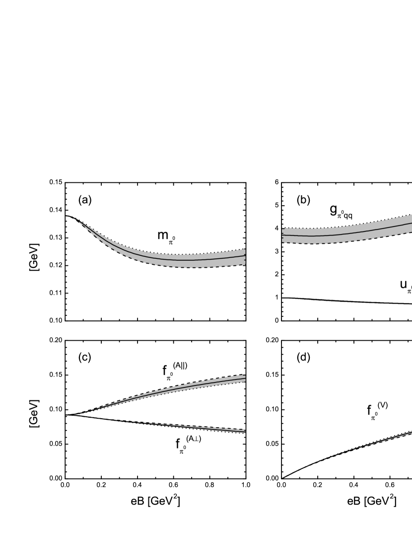
Figure 1: Neutral pion properties as functions of $eB$. Solid lines correspond to set I, while the limits of the gray bands correspond to set II (dashed lines) and set III (dotted lines).

It is interesting to notice that the numerical results given above (which have been obtained from parametrization sets leading to $m_{\pi^{0}}=138$ MeV at $B=0$) satisfy quite well the chiral limit relations in Eqs. (87-91). In fact, it is found that all these relations are satisfied at a level of less than 1% for all considered values of $eB$.

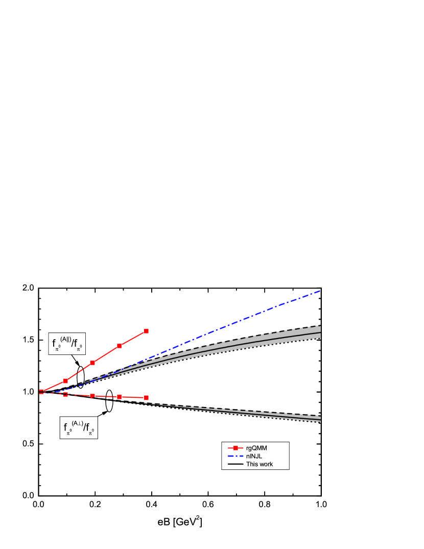
Figure 2: Neutral pion decay constants as functions of $eB$ for various models.

To conclude this subsection, in Fig. 2 we show a comparison between our results for the axial decay constants, normalized to the value at $B=0$, and the results obtained in Refs. GomezDumm:2017jij and Kamikado:2013pya . Those works are based on a nonlocal NJL model (nlNJL), dashed-dotted line in the figure, and on the functional renormalization group approach to the quark-meson model (rgQMM), red squares, respectively. We see that in the case of $f_{\pi^{0}}^{(A\parallel)}$ our results are somewhat below those obtained within the rgQMM. This is likely to be correlated with the fact that in that approach the $\pi^{0}$ mass shows a stronger decrease as the magnetic field increases. A similar trend is found for $f_{\pi^{0}}^{(A\perp)}$, although in this case the difference with the rgQMM calculation of Ref. Kamikado:2013pya is somewhat smaller. It should be mentioned that additional calculations for $f_{\pi^{0}}^{(A\parallel)}$ have been carried out using ChPT Andersen:2012zc and within the effective chiral confinement Lagrangian approach Andreichikov:2018wrc . The latter shows a behavior similar to that of the nlNJL model considered in Ref. GomezDumm:2017jij , while ChPT results, trustable for values of the magnetic field up to say $eB\sim 0.1$ GeV², are found to be in reasonable agreement with our curves.

IV.2 Charged pions

In Fig. 3 we show our numerical results for the quantities associated with charged pions, in the lowest Landau level (LLL), as functions of $eB$. As in the previous subsection, solid lines indicate the results for parameter set I, while the limits of the gray bands correspond to set II (dashed lines) and set III (dotted lines). From the figure it is observed that, as in the case of the $\pi^{0}$, the qualitative behavior of all calculated quantities is not significantly affected by changes in the model parametrization within the considered limits. In Fig. 3(a) we quote the results for the magnetic field-dependent charged pion mass, see Eq. (44), which have already been presented in Ref. Coppola:2018vkw . They are included here just for completeness. As discussed in Ref. Coppola:2018vkw , our results are in fair agreement with those obtained from LQCD Bali:2017ian , once the current quark mass is increased so that $m_{\pi^{+}}(B=0)$ matches the value of the pion mass considered in lattice calculations.

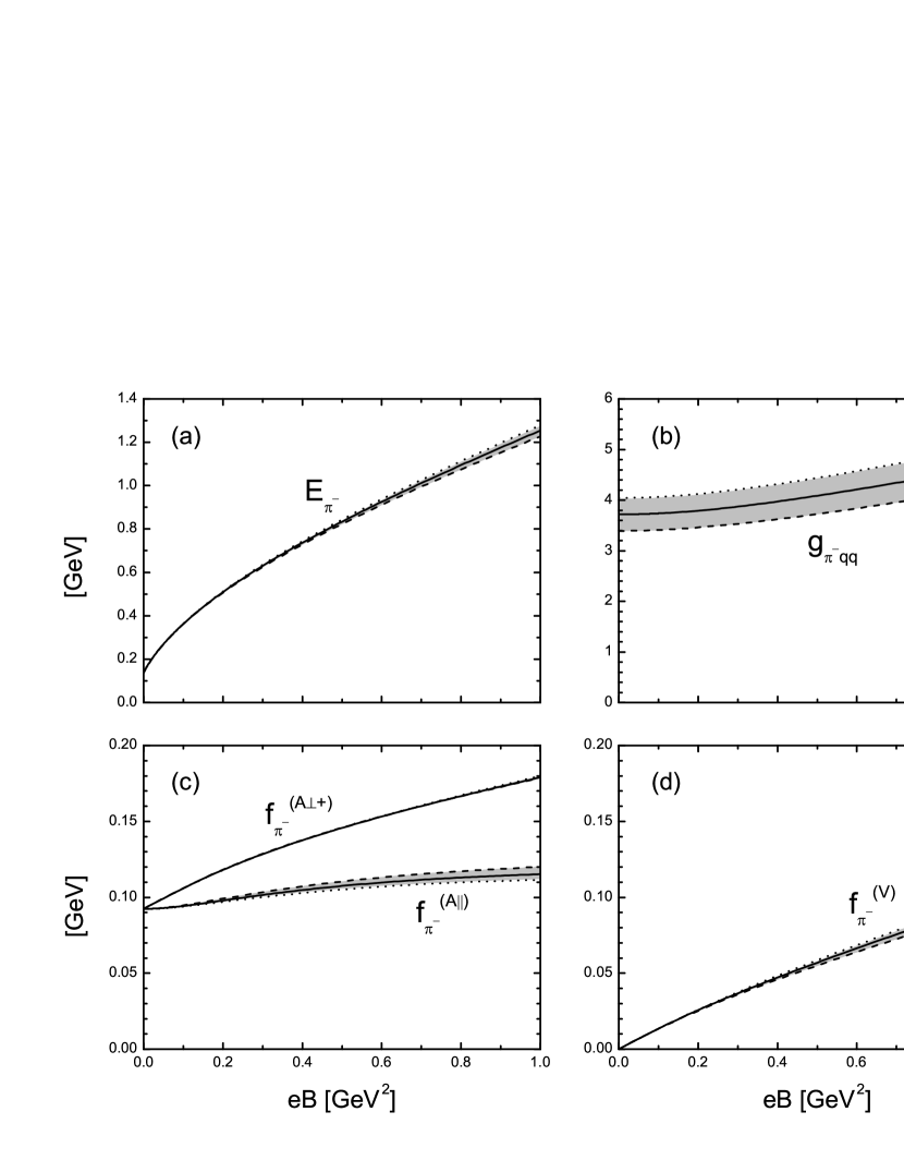
Figure 3: Charged pion decay properties as functions of $eB$. Solid lines correspond to set I, while the limits of the grey bands correspond to set II (dashed lines) and set III (dotted lines).

In Fig. 3(b) we quote the curves corresponding to the coupling constant $g_{\pi^{-}qq}$ as a function of $eB$. It can be seen that they are quite similar to those obtained for the neutral pion in Fig. 1(b). The behavior of the axial decay constants is shown in Fig. 3(c). We choose to plot $f_{\pi^{-}}^{(A\parallel)}$ (also denoted as $f_{\pi^{-}}^{(A1),({\rm reg})}$) and the combination $f_{\pi^{-}}^{(A\perp+)}=f_{\pi^{-}}^{(A1),({\rm reg})}+f_{\pi^{-}}^{(A2)}-f_{\pi^{-}}^{(A3)}$, since —as discussed in Sec. II— if the pion lies on the LLL these are the only relevant form factors for the evaluation of the matrix elements of the axial current. From the figure it is observed that $f_{\pi^{-}}^{(A\parallel)}$ shows a slight growth with $eB$, lower than that of $f_{\pi^{0}}^{(A\parallel)}$ [see Fig. 1(c)]. On the other hand, $f_{\pi^{-}}^{(A\perp+)}$ exhibits a strong increase with $eB$, reaching a magnitude of about 180 MeV for $eB=1$ GeV². Finally, in Fig. 3(d) we plot $f_{\pi^{-}}^{(V)}$ as a function of the magnetic field. Its behavior is similar to that of $f_{\pi^{0}}^{(V)}$, shown in Fig. 1(d).

In the framework of lattice QCD, some results for $f_{\pi^{-}}^{(A\parallel)}$ and $f_{\pi^{-}}^{(V)}$ in the presence of an external magnetic field have been presented recently Bali:2018sey . Although errors are still relatively large, it can be seen that beyond the first lattice data points $f_{\pi^{-}}^{(A\parallel)}$ shows an overall increase with the magnetic field, in qualitative agreement with our results. On the other hand, a continuum extrapolation seems to indicate that $f_{\pi^{-}}^{(A||)}$ starts out with a negative slope, which differs from the case of $f_{\pi^{0}}^{(A\parallel)}$. We find this result difficult to understand, since the decay constants of charged and neutral pions should behave similarly Andersen:2012zc for very small values of $eB$. In addition, in Ref. Dominguez:2018njv the magnetic field dependence of $f_{\pi^{-}}^{(A\parallel)}$ has been analyzed in the context of QCD sum rules. In comparison with our results, their analysis shows a steeper enhancement with $B$, leading to $f_{\pi^{-}}^{(A\parallel)}\sim 0.17$ GeV for $eB=1$ GeV². In any case, it should be stressed that our results show that, as expected, the Goldberger-Treiman and Gell-Mann-Oakes-Renner relations for charged pions [i.e., the equivalent to Eqs. (87) and (90), obtained for neutral mesons] are violated for $eB\gtrsim m_{\pi}^{2}$, for both $f_{\pi^{-}}^{(A\parallel)}$ and $f_{\pi^{-}}^{(A\perp+)}$.

To conclude, let us make an additional comment on the magnetic field dependences of the decay constants. In the chiral limit, it can be seen that for low values of $eB$ the difference $f_{\pi^{-}}^{(A2)}-f_{\pi^{-}}^{(A3)}$ is given by

$$f_{\pi^{-},\,{\rm ch}}^{(A2)}-f_{\pi^{-},\,{\rm ch}}^{(A3)}\ =\ \frac{eB}{8\pi^{2}f_{\pi^{-},\,{\rm ch}}^{(A\parallel)}}\,\Big{(}1\,-\,\frac{7\,eB}{45\,M_{\rm ch}^{2}}\,+\,\dots\Big{)}\ .$$ (93)

On the other hand, in the case of $f_{\pi^{-}}^{(V)}$, for low values of the magnetic field a relation similar to Eq. (91) is expected to be satisfied in the chiral limit. From our numerical calculations we find quite remarkable that relations of the same form, i.e.,

$$f_{\pi^{-}}^{(A2)}-f_{\pi^{-}}^{(A3)}\ =\ \frac{eB}{8\pi^{2}f_{\pi^{-}}^{(A\parallel)}}\,\Big{(}1\,-\,\frac{7\,eB}{45\,M^{2}}\Big{)}$$ (94)

and

$$f_{\pi^{-}}^{(V)}\ =\ \frac{eB}{8\pi^{2}f_{\pi^{-}}^{(A\parallel)}}\ ,$$ (95)

are in fact approximately valid also for large external magnetic fields. Indeed, although in the presence of the magnetic field the $\pi^{-}$ cannot be considered a pseudo-Goldstone boson, we find that $f_{\pi^{-}}^{(A2)}-f_{\pi^{-}}^{(A3)}$ and $f_{\pi^{-}}^{(V)}$ can be approximated by the expressions in Eqs. (94) and (95) within 15% and 10% accuracy, respectively, for values of $eB$ up to 1 GeV². It would be interesting to verify if equivalent relations also arise within other theoretical approaches to low energy hadron physics.

V Summary and conclusions

In this work we have considered the approach introduced in Ref. Coppola:2018vkw for the study of pion masses, extending the calculations to other properties of neutral and charged pions. Such an approach is based on the usage of the Nambu-Jona-Lasinio effective model for low energy QCD dynamics, in which pions are treated as quantum fluctuations in the random phase approximation. While for the $\pi^{0}$ one can take the usual momentum basis to diagonalize the corresponding polarization functions, this is not possible in the case of charged pions, due to the presence of nonvanishing contributions from Schwinger phases. Therefore, to diagonalize the charged pion polarization function we use a method based on the Ritus eigenfunction approach to magnetized relativistic systems. Since the NJL model is not renormalizable, the calculation of observables requires an appropriate regularization scheme in order to deal with ultraviolet divergences. Here, we have used the magnetic field independent regularization procedure, in which only divergent vacuum contributions to quantities at zero external magnetic field are regularized. This scheme has been shown to provide more reliable predictions in comparison with other regularization methods often used in the literature Avancini:2019wed . Within the framework just described, we have concentrated in particular on the analysis of the quark-meson coupling constants, the neutral pion directional refraction index $u_{\pi^{0}}$, and the form factors associated with pion-to-vacuum matrix elements of the vector and axial vector hadronic currents.

In the case of the neutral pion we find that while the coupling constant $g_{\pi^{0}qq}$ shows some enhancement if the external magnetic field is increased, $u_{\pi^{0}}$ decreases monotonously with $eB$, remaining always lower than one. We have checked that $u_{\pi^{0}}$ is kept almost unchanged if one takes $m_{0}\rightarrow 0$, which implies that, contrary to the result obtained in Ref. Fayazbakhsh:2013cha , for nonzero $B$ neutral pions move at a speed lower than the speed of light even in the chiral limit. Concerning the study of pion-to-vacuum amplitudes, in agreement with previous analyses Miransky:2002rp ; Kamikado:2013pya ; Fayazbakhsh:2012vr ; Coppola:2018ygv we find that for the $\pi^{0}$, in the presence of the external magnetic field, there are in general two axial nonvanishing form factors, namely $f_{\pi^{0}}^{(A\parallel)}$ and $f_{\pi^{0}}^{(A\perp)}$. Moreover, as discussed in Ref. Coppola:2018ygv , the vector hadronic current is also found to be nonvanishing, and an additional vector form factor $f_{\pi^{0}}^{(V)}$ can be defined. We have verified that in the chiral limit these quantities satisfy some relations. In fact, apart from the well-known generalized Goldberger-Treiman and Gell-Mann-Oakes-Renner equations for $f_{\pi^{0}}^{(A\parallel)}$ (see e.g. Ref. Agasian:2001ym ), we show that in that limit the relations $f_{\pi^{0}}^{(A\perp)}\ =\ u^{2}_{\pi^{0}}f_{\pi^{0}}^{(A\parallel)}$ and $f_{\pi^{0}}^{(V)}\ =\ eB/(8\pi^{2}f_{\pi^{0}}^{(A\parallel)})$ hold. The first of these equations follows from the expressions quoted in Ref. Fayazbakhsh:2013cha and can also be derived in the context of ChPT. On the other hand, the second one can be related to the anomalous Wess-Zumino-Witten effective lagrangian, and—to the best of our knowledge—has not been previously stated in the literature. Our numerical results for the neutral axial decay constants indicate that, starting from a common value at $B=0$, $f_{\pi^{0}}^{(A\parallel)}$ gets enhanced for increasing $eB$, while $f_{\pi^{0}}^{(A\perp)}$ gets reduced. We see that in the case of $f_{\pi^{0}}^{(A\parallel)}$ our results are somewhat below those obtained in Refs. Kamikado:2013pya ; GomezDumm:2017jij . This is likely to be correlated with the fact that in those approaches the $\pi^{0}$ mass shows a stronger decrease as the magnetic field increases. A similar trend is found for $f_{\pi^{0}}^{(A\perp)}$, although in this case the difference with the calculation of Ref. Kamikado:2013pya is somewhat smaller. It is interesting to notice that the numerical results for the form factors, obtained for model parameters leading to a physical $B=0$ pion mass, satisfy chiral limit relations in Eqs. (87-91) quite well (that is, within 1% for all considered values of $eB$).

For the charged pions we find that the $B$ dependence of the corresponding quark-meson coupling constant is quite similar to the one found in the case of the $\pi^{0}$. Concerning the axial form factors, we see that while in general three decay constants can be defined GomezDumm:2017jij , only two linear combinations of them, $f_{\pi^{-}}^{(A\parallel)}$ and $f_{\pi^{-}}^{(A\perp+)}$, are physically relevant for charged pions in their lowest energy state. As in the case of the $\pi^{0}$, we find that there is also a vector form factor $f_{\pi^{-}}^{(V)}$ that can be nonvanishing Bali:2018sey ; GomezDumm:2017jij . Our numerical results indicate that while $f_{\pi^{-}}^{(A\parallel)}$ shows a rather slight growth with the magnetic field (somewhat lower than that of $f_{\pi^{0}}^{(A\parallel)}$), $f_{\pi^{-}}^{(A\perp+)}$ exhibits a stronger increase with $eB$, reaching a magnitude of about 180 MeV for $eB=1$ GeV². Finally, it is seen that for $eB\lesssim 1$ GeV² the decay constants for the charged pion satisfy approximate relations that are equivalent to those obtained in the chiral limit for low values of the magnetic field.

APPENDIX A: DIRAC TRACES

In this appendix we provide the explicit form of the Dirac traces that appear in the calculation of the pion two-point functions and the pion-to-vacuum matrix elements. In all cases we use the Schwinger form of the propagators, with $\tilde{S}_{p}^{f}$ given by Eq. (15). As in the main text, we separate the four-vectors into parallel and perpendicular two-vectors, e.g. $p_{\perp}=(p_{1},p_{2})$ , $p_{\parallel}=(p_{3},p_{4})$.

The traces appearing in the two-point functions can be written as

$${\rm tr}_{D}\left[\tilde{S}_{p^{+}}^{f_{1}}\gamma_{5}\,\tilde{S}_{p^{-}}^{f_{2}}\gamma_{5}\right]\ =\ \int_{0}^{\infty}d\tau\int_{0}^{\infty}d\tau^{\prime}\ \exp\left[-\tau\phi_{f_{1}}(\tau,p^{+})-\tau^{\prime}\phi_{f_{2}}(\tau^{\prime},p^{-})\right]\,T_{5}\ ,$$ (96)

where

$$\phi_{f_{i}}(\tau,p^{\pm})\ =\ M^{2}\,+\,{p_{\parallel}^{\pm}\,}^{2}\,+\,\frac{t_{f_{i}}}{\tau B_{f}}\;{p_{\perp}^{\pm}\,}^{2}\ ,$$ (97)

with $t_{f_{i}}=\tanh(\tau B_{f_{i}})$. Writing $p^{\pm}=p\pm v/2$, from Eq. (15) one has

$$T_{5}\ =\ 4\,\left[\left(M^{2}+p_{\parallel}^{2}-\frac{v_{\parallel}^{2}}{4}\,\right)\,(1+s_{f_{1}}\,s_{f_{2}}\,t_{f_{1}}\,t^{\prime}_{f_{2}})\,+\,(1-t^{2}_{f_{1}})\,(1-{t^{\prime}_{f_{2}}}^{2})\,\left(p_{\perp}^{2}-\frac{v_{\perp}^{2}}{4}\right)\right]\ ,$$ (98)

where $t^{\prime}_{f_{i}}=\tanh(\tau^{\prime}B_{f_{i}})$. Similarly, for the traces appearing in the analysis of the pion-to-vacuum matrix elements we write

$${\rm tr}_{D}\left[\tilde{S}_{p^{+}}^{f_{1}}\gamma_{5}\,\tilde{S}_{p^{-}}^{f_{2}}\Gamma^{C}_{\mu}\right]\ =\ \int_{0}^{\infty}d\tau\int_{0}^{\infty}d\tau^{\prime}\ \exp\left[-\tau\phi_{f_{1}}(\tau,p^{+})-\tau^{\prime}\phi_{f_{2}}(\tau^{\prime},p^{-})\right]\,T^{C}_{\mu}\ .$$ (99)

Taking into account the linear combinations relevant for our calculations, we find

$$T_{\parallel}^{V,\epsilon} = T^{V}_{4}+\epsilon\,T^{V}_{3}\,=\,-4iM\,(v_{3}-\epsilon\,v_{4})\,\big{(}s_{f_{1}}\,t_{f_{1}}+s_{f_{2}}\,t^{\prime}_{f_{2}}\big{)}\ ,$$ (100)

$$T_{\parallel}^{A,\epsilon} = T^{A}_{4}+\epsilon\,T^{A}_{3}\,=\,-4M\,(v_{4}+\epsilon\,v_{3})\,\big{(}1\,+\,s_{f_{1}}\,s_{f_{2}}\,t_{f_{1}}\,t^{\prime}_{f_{2}}\big{)}\ ,$$ (101)

$$T_{\perp}^{V,\epsilon} = T^{V}_{1}+\epsilon\,i\,T^{V}_{2}\,=\,0\ ,$$ (102)

$$T_{\perp}^{A,\epsilon} = T^{A}_{1}+\epsilon\,i\,T^{A}_{2}\,=\,-4M\bigg{\{}\!(p_{1}+\epsilon\,ip_{2})\Big{[}(1-t_{f_{1}}^{2})\,(1+\epsilon\,s_{f_{2}}\,t^{\prime}_{f_{2}})-(1-t_{f_{2}}^{2})\,(1-\epsilon\,s_{f_{1}}\,t_{f_{1}})\Big{]}+$$ (103)

$$\frac{1}{2}\,(v_{1}+\epsilon\,iv_{2})\Big{[}(1-t_{f_{1}}^{2})\,(1+\epsilon\,s_{f_{2}}\,t^{\prime}_{f_{2}})+(1-{t^{\prime}_{f_{2}}}^{2})\,(1-\epsilon\,s_{f_{1}}\,t_{f_{1}})\Big{]}\bigg{\}}\ .$$

APPENDIX B: INTEGRALS OVER INTERNAL MOMENTA

The integrals in Eqs. (37) and (76) can be performed using the properties of the cylindrical parabolic functions $D_{k}(x)$. We need to calculate

$$I_{\lambda}\ =\ \int_{p\,v_{\perp}}e^{-\tau\phi_{f_{1}}(\tau,p^{+})}\,e^{-\tau^{\prime}\phi_{f_{2}}(\tau^{\prime},p^{-})}\,e^{iv_{1}(x_{1}-x^{\prime}_{1})}\,D_{k}(\sqrt{2B_{e}}\,x^{\prime}_{1}+\sqrt{2/B_{e}}\,q^{\prime}_{2})\;T_{\lambda}\ ,$$ (104)

where $T_{\lambda}$ stands for the functions $T_{5}$, $T_{\parallel}^{C,\epsilon}$ and $T_{\perp}^{C,\epsilon}$ in Appendix A.

The integrals over $p_{\parallel}$ can be easily obtained from the relations

$$\int_{p_{\parallel}}e^{-a(p_{\parallel}+v_{\parallel}/2)^{2}}\,e^{-b(p_{\parallel}-v_{\parallel}/2)^{2}} = \frac{1}{4\pi(a+b)}\;e^{-\frac{ab}{a+b}\;v_{\parallel}^{2}}\ ,$$

$$\int_{p_{\parallel}}\left(p_{\parallel}^{2}-\frac{v_{\parallel}^{2}}{4}\right)\;e^{-a(p_{\parallel}+v_{\parallel}/2)^{2}}\,e^{-b(p_{\parallel}-v_{\parallel}/2)^{2}} = \frac{1}{4\pi(a+b)^{2}}\,\Big{[}1-\frac{ab}{a+b}\;v_{\parallel}^{2}\Big{]}\,e^{-\frac{ab}{a+b}\;v_{\parallel}^{2}}\ .$$ (105)

These expressions can be also applied for the integrals over $p_{\perp}$. For the case of $T_{\perp}^{A,\epsilon}$ we also need

$$\int_{p_{\perp}}(p_{1}+\epsilon\,ip_{2})\,e^{-a(p_{\perp}+v_{\perp}/2)^{2}-b(p_{\perp}-v_{\perp}/2)^{2}}\ =\ -\,\frac{1}{8\pi}\,(v_{1}+\epsilon\,iv_{2})\,\frac{(a-b)\;}{(a+b)^{2}}\;e^{-\frac{ab}{a+b}\;v_{\perp}^{2}}\ .$$ (106)

On the other hand, the integrals over $v_{\perp}$ can be obtained taking into account the following useful relations. Defining

$${\cal D}_{k}(x_{1},q_{2},v_{\perp})\ =\ D_{k}(\sqrt{2B_{e}}\,x^{\prime}_{1}+\sqrt{2/B_{e}}\,q_{2})\;e^{iv_{1}(x_{1}-x^{\prime}_{1})}\,\Big{|}_{x_{1}^{\prime}=-x_{1}+2(v_{2}-q_{2})/B_{e}}\ \ ,$$ (107)

one has

$$\int_{v_{\perp}}{\cal D}_{k}(x_{1},q_{2},v_{\perp})\;e^{-\gamma v_{\perp}^{2}} = \frac{B_{e}}{4\pi}\,\frac{(1-\gamma B_{e})^{k}}{(1+\gamma B_{e})^{k+1}}\,D_{k}(\sqrt{2B_{e}}\,x_{1}+\sqrt{2/B_{e}}\,q_{2})\ ,$$

$$\int_{v_{\perp}}(v_{1}+\epsilon\,iv_{2})\,{\cal D}_{k}(x_{1},q_{2},v_{\perp})\;e^{-\gamma v_{\perp}^{2}} = \frac{i\,\epsilon\sqrt{2}\,B_{e}^{3/2}}{4\pi}\,\Big{(}\frac{1-\gamma B_{e}}{1+\gamma B_{e}}\Big{)}^{k+\epsilon}\frac{k^{(1-\epsilon)/2}}{(1+\gamma B_{e})\,(1-\epsilon\gamma B_{e})}\,\times$$

$$D_{k+\epsilon}(\sqrt{2B_{e}}\,x_{1}+\sqrt{2/B_{e}}\,q_{2})\ ,$$

$$\int_{v_{\perp}}\,v_{\perp}^{2}\,{\cal D}_{k}(x_{1},q_{2},v_{\perp})\;e^{-\gamma v_{\perp}^{2}} = \frac{B_{e}^{2}}{4\pi}\,\frac{(1-\gamma B_{e})^{k-1}}{(1+\gamma B_{e})^{k+2}}\,(1-\gamma B_{e}+2k)\,\times$$ (108)

$$D_{k}(\sqrt{2B_{e}}\,x_{1}+\sqrt{2/B_{e}}\,q_{2})\ .$$

References

• (1) D. E. Kharzeev, K. Landsteiner, A. Schmitt and H. U. Yee, Lect. Notes Phys.  871, 1 (2013).
• (2) J. O. Andersen, W. R. Naylor and A. Tranberg, Rev. Mod. Phys.  88, 025001 (2016).
• (3) V. A. Miransky and I. A. Shovkovy, Phys. Rep.  576, 1 (2015).
• (4) D. Grasso and H. R. Rubinstein, Phys. Rep.  348, 163 (2001).
• (5) D. E. Kharzeev, L. D. McLerran and H. J. Warringa, Nucl. Phys. A 803, 227 (2008); V. Skokov, A. Y. Illarionov, and V. Toneev, Int. J. Mod. Phys. A 24, 5925 (2009); V. Voronyuk, V. Toneev, W. Cassing, E. Bratkovskaya, V. Konchakovski, and S. Voloshin, Phys. Rev. C 83, 054911 (2011).
• (6) R. C. Duncan and C. Thompson, Astrophys. J. 392, L9 (1992); C. Kouveliotou et al., Nature (London) 393, 235 (1998).
• (7) S. Fayazbakhsh, S. Sadeghian and N. Sadooghi, Phys. Rev. D 86, 085042 (2012).
• (8) S. Fayazbakhsh and N. Sadooghi, Phys. Rev. D 88, 065030 (2013).
• (9) S. S. Avancini, W. R. Tavares and M. B. Pinto, Phys. Rev. D 93, 014010 (2016).
• (10) S. S. Avancini, R. L. S. Farias, M. Benghi Pinto, W. R. Tavares and V. S. Timoteo, Phys. Lett. B 767, 247 (2017).
• (11) S. Mao and Y. Wang, Phys. Rev. D 96, 034004 (2017).
• (12) R. Zhang, W. j. Fu and Y. x. Liu, Eur. Phys. J. C 76, 307 (2016).
• (13) D. Gomez Dumm, M. F. I. Villafañe and N. N. Scoccola, Phys. Rev. D 97, 034025 (2018).
• (14) Z. Wang and P. Zhuang, Phys. Rev. D 97, 034026 (2018).
• (15) H. Liu, X. Wang, L. Yu and M. Huang, Phys. Rev. D 97, 076008 (2018).
• (16) M. Coppola, D. Gomez Dumm and N. N. Scoccola, Phys. Lett. B 782, 155 (2018).
• (17) S. Mao, Phys. Rev. D 99, 056005 (2019).
• (18) S. S. Avancini, R. L. S. Farias and W. R. Tavares, Phys. Rev. D 99, 056009 (2019).
• (19) A. Ayala, R. L. S. Farias, S. Hernández-Ortiz, L. A. Hernández, D. M. Paret and R. Zamora, Phys. Rev. D 98, 114008 (2018).
• (20) K. Kamikado and T. Kanazawa, JHEP 1403, 009 (2014).
• (21) N. O. Agasian and I. A. Shushpanov, JHEP 0110, 006 (2001).
• (22) J. O. Andersen, JHEP 1210, 005 (2012).
• (23) G. Colucci, E. S. Fraga and A. Sedrakian, Phys. Lett. B 728, 19 (2014).
• (24) V. D. Orlovsky and Y. A. Simonov, JHEP 1309, 136 (2013).
• (25) M. A. Andreichikov, B. O. Kerbikov, E. V. Luschevskaya, Y. A. Simonov and O. E. Solovjeva, JHEP 1705, 007 (2017).
• (26) Y. A. Simonov, Phys. Atom. Nucl.  79, 455 (2016) [Yad. Fiz.  79, 277 (2016)].
• (27) M. A. Andreichikov and Y. A. Simonov, Eur. Phys. J. C 78, 902 (2018).
• (28) C. A. Dominguez, M. Loewe and C. Villavicencio, Phys. Rev. D 98, 034015 (2018).
• (29) G. S. Bali, F. Bruckmann, G. Endrodi, Z. Fodor, S. D. Katz, S. Krieg, A. Schafer and K. K. Szabo, JHEP 1202, 044 (2012).
• (30) Y. Hidaka and A. Yamamoto, Phys. Rev. D 87, 094502 (2013).
• (31) E. V. Luschevskaya, O. E. Solovjeva, O. A. Kochetkov and O. V. Teryaev, Nucl. Phys. B 898, 627 (2015).
• (32) B. B. Brandt, G. Bali, G. Endrodi and B. Glaessle, PoS LATTICE 2015, 265 (2016).
• (33) G. S. Bali, B. B. Brandt, G. Endrodi and B. Glaessle, Phys. Rev. D 97, 034505 (2018).
• (34) U. Vogl and W. Weise, Prog. Part. Nucl. Phys. 27, 195 (1991).
• (35) S. P. Klevansky, Rev. Mod. Phys.  64, 649 (1992).
• (36) T. Hatsuda and T. Kunihiro, Phys. Rep.  247, 221 (1994).
• (37) J. S. Schwinger, Phys. Rev.  82, 664 (1951).
• (38) V. I. Ritus, Sov. Phys. JETP 48, 788 (1978).
• (39) S. S. Avancini, R. L. S. Farias, N. N. Scoccola and W. R. Tavares, Phys. Rev. D 99, 116002 (2019).
• (40) G. S. Bali, B. B. Brandt, G. Endrődi and B. Gläßle, Phys. Rev. Lett.  121, 072001 (2018).
• (41) M. Coppola, D. Gomez Dumm, S. Noguera and N. N. Scoccola, Phys. Rev. D 99, 054031 (2019).
• (42) D. P. Menezes, M. Benghi Pinto, S. S. Avancini, A. Perez Martinez and C. Providencia, Phys. Rev. C 79, 035807 (2009).
• (43) P. G. Allen, A. G. Grunfeld and N. N. Scoccola, Phys. Rev. D 92, 074041 (2015).
• (44) V. A. Miransky and I. A. Shovkovy, Phys. Rev. D 66, 045006 (2002).
• (45) J. Wess and B. Zumino, Phys. Lett.  37B, 95 (1971); E. Witten, Nucl. Phys. B 223, 422 (1983).
• (46) V. P. Gusynin, V. A. Miransky and I. A. Shovkovy, Nucl. Phys. B 462, 249 (1996).
• (47) K. Fukushima and Y. Hidaka, Phys. Rev. Lett.  110, 031601 (2013).