Dual Extrapolation for Sparse Generalized Linear Models

Abstract

Generalized Linear Models (GLM) form a wide class of regression and classification models, where prediction is a function of a linear combination of the input variables. For statistical inference in high dimension, sparsity inducing regularizations have proven to be useful while offering statistical guarantees. However, solving the resulting optimization problems can be challenging: even for popular iterative algorithms such as coordinate descent, one needs to loop over a large number of variables. To mitigate this, techniques known as screening rules and working sets diminish the size of the optimization problem at hand, either by progressively removing variables, or by solving a growing sequence of smaller problems. For both techniques, significant variables are identified thanks to convex duality arguments. In this paper, we show that the dual iterates of a GLM exhibit a Vector AutoRegressive (VAR) behavior after sign identification, when the primal problem is solved with proximal gradient descent or cyclic coordinate descent. Exploiting this regularity, one can construct dual points that offer tighter certificates of optimality, enhancing the performance of screening rules and working set algorithms.

Keywords: Convex optimization, extrapolation, screening rules, working sets, Lasso, sparse logistic regression, generalized linear models

1 Introduction

Since the introduction of the Lasso (Tibshirani, 1996), similar to the Basis Pursuit denoising (Chen and Donoho, 1995) in signal processing, sparsity inducing penalties have had a tremendous impact on machine learning (Bach et al., 2012). They have been applied to a variety of statistical estimators, both for regression and classification tasks: sparse logistic regression (Koh et al., 2007), Group Lasso (Yuan and Lin, 2006), Sparse Group Lasso (Simon et al., 2013), multitask Lasso (Obozinski et al., 2010), Square-Root Lasso (Belloni et al., 2011). All of these estimators fall under the framework of Generalized Linear Models (McCullagh and Nelder, 1989), where the output is assumed to follow an exponential family distribution whose mean is a linear combination of the input variables. The key property of $\ell_{1}$ regularization is that it allows to jointly perform feature selection and prediction, which is particularly useful in high dimensional settings. Indeed, it can drastically reduce the number of variables needed for prediction, thus improving model interpretability and computation time for prediction. Amongst the algorithms proposed to solve these, coordinate descent (Tseng, 2001; Friedman et al., 2007) is the most popular in machine learning scenarios (Fan et al., 2008; Friedman et al., 2010; Richtárik and Takáč, 2014; Fercoq and Richtárik, 2015; Perekrestenko et al., 2017; Karimireddy et al., 2018). It consists in updating the vector of parameters one coefficient at a time, looping over all the predictors until convergence.

Since only a fraction of the coefficients are non-zero in the optimal parameter vector, a recurring idea to speed up solvers is to limit the size of the optimization problem by ignoring features which are not included in the solution. To do so, two approaches can be distinguished:

• screening rules, introduced by El Ghaoui et al. (2012) and later developed by Ogawa et al. (2013); Wang et al. (2012); Xiang et al. (2016); Bonnefoy et al. (2014); Fercoq et al. (2015); Ndiaye et al. (2016, 2017), progressively remove features from the problems in a backward approach,

• working sets techniques (Fan and Lv, 2008; Roth and Fischer, 2008; Kowalski et al., 2011; Tibshirani et al., 2012; Johnson and Guestrin, 2015) solve a sequence of smaller problems restricted to a growing number of features.

One common idea between the current state-of-art methods for screening (Gap Safe rules Fercoq et al. 2015; Ndiaye et al. 2017) and working sets (Blitz, Johnson and Guestrin 2015, 2018) is to rely heavily on a dual point to identify useful features. The quality of such a dual point for the dual problem is critical here as it has a direct impact on performance. However, although a lot of attention has been devoted to creating a sequence of primal iterates that converge fast to the optimum (Fercoq and Richtárik, 2015), the construction of dual iterates has not been scrutinized, and the standard approach to obtain dual iterates from primal ones (Mairal, 2010), although converging, is crude.

In this paper, we propose a principled way to construct a sequence of dual points that converges faster than the standard approach proposed by Mairal (2010). Based on an extrapolation procedure inspired by Scieur et al. (2016), it comes with no significant extra computational costs, while retaining convergence guarantees of the standard approach. This construction was first introduced for non-smooth optimization by Massias et al. (2018) for the Lasso case only, while we generalize it here to any Generalized Linear Model (GLM). More precisely, we properly define, quantify and prove the asymptotic Vector AutoRegressive (VAR) behavior of dual iterates for sparse GLMs solved with proximal gradient descent or cyclic coordinate descent. The resulting new construction:

• provides a tighter control of optimality through duality gap evaluation,

• improves the performance of Gap safe rules,

• is easy to implement and combine with other solvers.

The article proceeds as follows. We introduce the framework of $\ell_{1}$-regularized GLMs and duality in Section 2. As a seminal example, we present our results on dual iterates regularity and dual extrapolation for the Lasso in Section 3. We generalize it to a variety of problems in Sections 4 and 5. Results of Section 6 demonstrate a systematic improvement in computing time when dual extrapolation is used together with Gap Safe rules or working set policies.

Notation

For any integer $d\in\mathbb{N}$, we denote by $[d]$ the set $\{1,\dots,d\}$. The design matrix $X\in\mathbb{R}^{n\times p}$ is composed of observations $\mathbf{x}_{i}\in\mathbb{R}^{p}$ stored row-wise, and whose $j$-th column is $x_{j}\in\mathbb{R}^{n}$; the vector $y\in\mathbb{R}^{n}$ (resp. $\{-1,1\}^{n}$) is the response vector for regression (resp. binary classification). The support of $\beta\in\mathbb{R}^{p}$ is $\mathcal{S}(\beta)=\{j\in[p]\,:\,\beta_{j}\neq 0\}$, of cardinality $\lVert{\beta}\rVert_{0}$. For $\mathcal{W}\subset[p]$, $\beta_{\mathcal{W}}$ and $X_{\mathcal{W}}$ are $\beta$ and $X$ restricted to features in $\mathcal{W}$. As much as possible, exponents between parenthesis (e.g., $\beta^{(t)}$) denote iterates and subscripts (e.g., $\beta_{j}$) denote vector entries or matrix columns. The sign function is $\operatorname{sign}:x\mapsto x/\lvert x\rvert$ with the convention $0/0=0$. The sigmoid function is $\sigma:x\mapsto 1/(1+e^{-x})$. The soft-thresholding of $x$ at level $\nu$ is $\operatorname{ST}(x,\nu)=\operatorname{sign}(x)\cdot\max(0,\left\lvert x\right\rvert-\nu)$. Applied to vectors, $\operatorname{sign}$, $\sigma$ and $\operatorname{ST}(\cdot,\nu)$ (for $\nu\in\mathbb{R}_{+}$) act element-wise. Element-wise product between vectors of same length is denoted by $\odot$. The vector of size $n$ whose entries are all equal to 0 (resp. 1) is denoted by $\mathbf{0}_{n}$ (resp. $\mathbf{1}_{n}$). On square matrices, $\lVert{\cdot}\rVert_{2}$ is the spectral norm (and the standard Euclidean norm for vectors reads $\left\lVert{\cdot}\right\rVert$); $\lVert{\cdot}\rVert_{1}$ is the $\ell_{1}$-norm. For a symmetric positive definite matrix $H$, $\langle x,y\rangle_{H}=x^{\top}Hy$ is the $H$-weighted inner product, whose associated norm is denoted $\lVert{\cdot}\rVert_{H}$. We extend the small-$o$ notation to vector valued functions in the following way: for $f:\mathbb{R}^{n}\to\mathbb{R}^{n}$ and $g:\mathbb{R}^{n}\to\mathbb{R}^{n}$, $f=o(g)$ if and only if $\lVert{f}\rVert=o(\lVert{g}\rVert)$, i.e., $\lVert{f}\rVert/\lVert{g}\rVert$ tends to 0 when $\lVert{g}\rVert$ tends to 0. For a convex and proper function $f:\mathbb{R}^{n}\to\mathbb{R}\cup\{\infty\}$, its Fenchel-Legendre conjugate $f^{*}:\mathbb{R}^{n}\to\mathbb{R}\cup\{\infty\}$ is defined by $f^{*}(u)=\sup_{x\in\mathbb{R}^{n}}u^{\top}x-f(x)$, and its subdifferential at $x\in\mathbb{R}^{n}$ is $\partial f(x)=\{u\in\mathbb{R}^{n}\,:\,\forall y\in\mathbb{R}^{n},f(y)\geq f(x)+u^{\top}(y-x)\}$.

2 GLMs, Vector AutoRegressive sequences and sign identification

We first introduce the class of optimization problems we consider.

Definition 1 (Sparse Generalized Linear Model).

We call Sparse Generalized Linear Model the following optimization problem:

$$\hat{\beta}\in\mathop{\mathrm{arg\,min}}_{\beta\in\mathbb{R}^{p}}\underbrace{\sum_{i=1}^{n}f_{i}(\beta^{\top}\mathbf{x}_{i})+\lambda\lVert{\beta}\rVert_{1}}_{\mathcal{P}(\beta)}\enspace,$$ (0)

where all $f_{i}$ are convex, differentiable functions with $1/\gamma$-Lipschitz gradients. The parameter $\lambda$ is a non-negative scalar, controlling the trade-off between data fidelity and regularization.

Two popular instances of (0) are the Lasso ($f_{i}(t)=\tfrac{1}{2}(y_{i}-t)^{2}$, $\gamma=1$) and Sparse Logistic regression ($f_{i}(t)=\log(1+\exp(-y_{i}t))$, $\gamma=4$); our naming is an abuse of language since for some choice of $f_{i}$’s, e.g., an Huber loss, there is no underlying statistical GLM.

A more complex regularizer could be used in (0), to handle group penalties for example. For the sake of clarity we rather remain specific, and generalize to other penalties when needed in Section 4.2.

Proposition 2 (Duality for sparse GLMs).

A dual formulation of (0) reads:

$$\hat{\theta}=\mathop{\mathrm{arg\,max}}_{\theta\in\Delta_{X}}\underbrace{\left(-\sum_{i=1}^{n}f_{i}^{*}(-\lambda\theta_{i})\right)}_{\mathcal{D}(\theta)}\enspace,$$ (0)

where $\Delta_{X}=\{\theta\in\mathbb{R}^{n}\,:\,\lVert{X^{\top}\theta}\rVert_{\infty}\leq 1\}$. The dual solution $\hat{\theta}$ is unique because the $f_{i}^{*}$’s are $\gamma$-strongly convex (Hiriart-Urruty and Lemaréchal, 1993, Thm 4.2.1) and the KKT conditions read:

$$\forall i\in[n],\quad\quad \,\hat{\theta}_{i}=-f_{i}^{\prime}(\hat{\beta}^{\top}\mathbf{x}_{i})/\lambda$$ (link equation) (1)

$$\forall j\in[p],\quad\quad \,x_{j}^{\top}\hat{\theta}\in\partial\lvert\cdot\rvert(\hat{\beta}_{j})$$ (subdifferential inclusion) (2)

If for $u\in\mathbb{R}^{n}$ we write $F(u)\stackrel{{\scriptstyle\mbox{\tiny def.}}}{{=}}\sum_{i=1}^{n}f_{i}(u_{i})$, the link equation reads $\hat{\theta}=-\nabla F(X\hat{\beta})/\lambda$.

For any $(\beta,\theta)\in\mathbb{R}^{p}\times\Delta_{X}$, one has $\mathcal{D}(\theta)\leq\mathcal{P}(\beta)$, and $\mathcal{D}(\hat{\theta})=\mathcal{P}(\hat{\beta})$. The duality gap $\mathcal{P}(\beta)-\mathcal{D}(\theta)$ can thus be used as an upper bound for the sub-optimality of a primal vector $\beta$: for any $\epsilon>0$, any $\beta\in\mathbb{R}^{p}$, and any feasible $\theta\in\Delta_{X}$:

$$\mathcal{P}(\beta)-\mathcal{D}(\theta)\leq\epsilon\Rightarrow\mathcal{P}(\beta)-\mathcal{P}(\hat{\beta})\leq\epsilon\enspace.$$ (3)

These results holds because Slater’s condition is met: (0) is unconstrained and the objective function has domain $\mathbb{R}^{p}$ (Boyd and Vandenberghe, 2004, §5.2.3), therefore strong duality holds.

Remark 3.

Equation 3 shows that even though $\hat{\beta}$ is unknown in practice and the sub-optimality gap cannot be evaluated, creating a dual feasible point $\theta\in\Delta_{X}$ allows to compute an upper bound which can be used as a tractable stopping criterion.

In high dimension, solvers such as proximal gradient descent (PG) and coordinate descent (CD) are slowed down due to the large number of features. However, by design of the $\ell_{1}$ penalty, $\hat{\beta}$ is known to be sparse, especially for large values of $\lambda$. Thus, a key idea to speed up these solvers is to identify the support of $\hat{\beta}$ so that features outside of it can be safely ignored: this leads to a smaller problem that is faster to solve. Removing features when it is guaranteed that they are not in the support of the solution is at the heart of the so-called Gap Safe Screening rules (Fercoq et al., 2015; Ndiaye et al., 2017).

Proposition 4 (Gap Safe Screening rule, (Ndiaye et al., 2017, Thm. 6)).

The Gap Safe screening rule for (0) reads:

$$\forall j\in[p],\forall\beta\in\mathbb{R}^{p},\forall\theta\in\Delta_{X},\,\frac{1-\lvert x_{j}^{\top}\theta\rvert}{\lVert{x_{j}}\rVert}>\sqrt{\tfrac{2}{\gamma\lambda^{2}}(\mathcal{P}(\beta)-\mathcal{D}(\theta))}\implies\hat{\beta}_{j}=0\enspace.$$ (4)

Therefore, while running an iterative solver, the criterion (4) can be tested periodically for all features $j$, and the features guaranteed to be inactive at optimum can be ignored.

Equations 3 and 4 do not require a specific choice of $\theta$, provided it is in $\Delta_{X}$. It is up to the user and so far it has not attracted much attention in the literature. Thanks to the link equation $\hat{\theta}=-\nabla F(X\hat{\beta})/\lambda$, a natural way to construct a dual feasible point $\theta^{(t)}\in\Delta_{X}$ at iteration $t$, when only a primal vector $\beta^{(t)}$ is available, is:

$$\theta_{\mathrm{res}}^{(t)}\stackrel{{\scriptstyle\mbox{\tiny def.}}}{{=}}-\nabla F(X\beta^{(t)})/\max(\lambda,\lVert{X^{\top}\nabla F(X\beta^{(t)})}\rVert_{\infty})\enspace.$$ (5)

This was coined residuals rescaling (Mairal, 2010) following the terminology used for the Lasso case where $-\nabla F(X\beta)$ is equal to the residuals, $y-X\beta$.

To improve the control of sub-optimality and identification of useful features, the aim of our proposed dual extrapolation is to obtain a better dual point (i.e., closer to the optimum $\hat{\theta}$). The idea is to do it at a low computational cost by exploiting the structure of the sequence of dual iterates $(X\beta^{(t)})_{t\in\mathbb{N}}$; we explain what is this “structure”, and how to exploit it, in the following.

Definition 5 (Vector AutoRegressive sequence).

We say that $(r^{(t)})_{t\in\mathbb{N}}\in(\mathbb{R}^{n})^{\mathbb{N}}$ is a Vector AutoRegressive (VAR) sequence (of order 1) if there exists $A\in\mathbb{R}^{n\times n}$ and $b\in\mathbb{R}^{n}$ such that for $t\in\mathbb{N}$:

$$r^{(t+1)}=Ar^{(t)}+b\enspace.$$ (6)

We also say that the sequence $(r^{(t)})_{t\in\mathbb{N}}$, converging to $\hat{r}$, is an asymptotic VAR sequence if there exist $A\in\mathbb{R}^{n\times n}$ and $b\in\mathbb{R}^{n}$ such that for $t\in\mathbb{N}$:

$$r^{(t+1)}-Ar^{(t)}-b=o(r^{(t)}-\hat{r})\enspace.$$ (7)

Proposition 6 (Extrapolation for VAR sequences (Scieur, 2018, Thm 3.2.2)).

Let $(r^{(t)})_{t\in\mathbb{N}}$ be a VAR sequence in $\mathbb{R}^{n}$, satisfying $r^{(t+1)}=Ar^{(t)}+b$ with $A\in\mathbb{R}^{n\times n}$ a symmetric positive definite matrix such that $\lVert{A}\rVert_{2}<1$, $b\in\mathbb{R}^{n}$ and $K<n$. Assume that for $t\geq K$, the family $\{r^{(t-K)}-r^{(t-K+1)},\ldots,r^{(t-1)}-r^{(t)}\}$ is linearly independent and define

$$U^{(t)} \stackrel{{\scriptstyle\mbox{\tiny def.}}}{{=}}[r^{(t-K)}-r^{(t-K+1)},\ldots,r^{(t-1)}-r^{(t)}]\in\mathbb{R}^{n\times K}\enspace,$$ (8)

$$(c_{1},\dots,c_{K}) \stackrel{{\scriptstyle\mbox{\tiny def.}}}{{=}}\frac{(U^{(t)}{}^{\top}U^{(t)}){}^{-1}\mathbf{1}_{K}}{\mathbf{1}_{K}^{\top}(U^{(t)}{}^{\top}U^{(t)}){}^{-1}\mathbf{1}_{K}}\in\mathbb{R}^{K}\enspace,$$ (9)

$$r_{\mathrm{extr}} \stackrel{{\scriptstyle\mbox{\tiny def.}}}{{=}}\sum_{k=1}^{K}c_{k}r^{(t-K-1+k)}\in\mathbb{R}^{n}\enspace.$$ (10)

Then, $r_{\mathrm{extr}}$ satisfies

$$\left\lVert{Ar_{\mathrm{extr}}-b-r_{\mathrm{extr}}}\right\rVert\leq\mathcal{O}(\rho^{K})\enspace,$$ (11)

where $\rho=\frac{1-\sqrt{1-\lVert{A}\rVert_{2}}}{1+\sqrt{1-\lVert{A}\rVert_{2}}}<1$.

The justification for this extrapolation procedure is the following: since $\lVert{A}\rVert_{2}<1$, $(r^{(t)})_{t\in\mathbb{N}}$ converges, say to $\hat{r}$. For $t\in\mathbb{N}$, we have $r^{(t+1)}-\hat{r}=A(r^{(t)}-\hat{r})$. Let $(a_{0},\dots,a_{n})\in\mathbb{R}^{n+1}$ be the coefficients of $A$’s characteristic polynomial. By Cayley-Hamilton’s theorem, $\sum_{k=0}^{n}a_{k}A^{k}=0$. Given that $\lVert{A}\rVert_{2}<1$, $1$ is not an eigenvalue of $A$ and $\sum_{k=0}^{n}a_{k}\neq 0$, so we can normalize these coefficients to have $\sum_{k=0}^{n}a_{k}=1$. For $t\geq n$, we have:

$$\sum_{k=0}^{n}a_{k}\left(r^{(t-n+k)}-\hat{r}\right) =\left(\sum_{k=0}^{n}a_{k}A^{k}\right)(r^{(t-n)}-\hat{r})=0\enspace,$$ (12)

$$\mathrm{and~{}so}\quad\quad\sum_{k=0}^{n}a_{k}r^{(t-n+k)} =\sum_{k=0}^{n}a_{k}\hat{r}=\hat{r}\enspace.$$ (13)

Hence, $\hat{r}\in\operatorname{Span}(r^{(t-n)},\dots,r^{(t)})$.

Therefore, it is natural to seek to approximate $\hat{r}$ as an affine combination of the $(n+1)$ last iterates $(r^{(t-n)},\dots,r^{(t)})$. Using $(n+1)$ iterates might be costly for large $n$, so one might rather consider only a smaller number $K$, i.e., find $(c_{1},\dots,c_{K})\in\mathbb{R}^{K}$ such that $\sum_{k=1}^{K}c_{k}r^{(t-K-1+k)}$ approximates $\hat{r}$. Since $\hat{r}$ is a fixed point of $r\mapsto Ar+b$, $\sum_{k=1}^{K}c_{k}r^{(t-K-1+k)}$ should be one too. Under the normalizing condition $\sum_{k=1}^{K}c_{k}=1$, this means that

$$\sum_{k=1}^{K}c_{k}r^{(t-K-1+k)}-A\sum_{k=1}^{K}c_{k}r^{(t-K-1+k)}-b =\sum_{k=1}^{K}c_{k}r^{(t-K-1+k)}-\sum_{k=1}^{K}c_{k}\left(r^{(t-K+k)}-b\right)-b$$

$$=\sum_{k=1}^{K}c_{k}\left(r^{(t-K-1+k)}-r^{(t-K+k)}\right)$$ (14)

should be as close to $\mathbf{0}_{n}$ as possible; this leads to solving:

$$\hat{c}=\mathop{\mathrm{arg\,min}}_{\begin{subarray}{c}c\in\mathbb{R}^{K}\\ c^{\top}\mathbf{1}_{K}=1\end{subarray}}\left\lVert{\sum_{k=1}^{K}c_{k}\left(r^{(t-K+k)}-r^{(t-K-1+k)}\right)}\right\rVert\enspace,$$ (15)

which admits a closed-form solution if $U^{(t)}\stackrel{{\scriptstyle\mbox{\tiny def.}}}{{=}}[r^{(t-K+1)}-r^{(t-K)},\ldots,r^{(t)}-r^{(t-1)}]\in\mathbb{R}^{n\times K}$ has full column rank (Scieur et al., 2016, Lemma 2.4):

$$\hat{c}=\frac{(U^{(t)}{}^{\top}U^{(t)}){}^{-1}\mathbf{1}_{K}}{\mathbf{1}_{K}^{\top}(U^{(t)}{}^{\top}U^{(t)}){}^{-1}\mathbf{1}_{K}}\enspace.$$ (16)

In practice, the next proposition shows that when $U^{(t)}$ does not have full column rank, it is theoretically sound to use a lower value for the number of extrapolation coefficients $K$.

Proposition 7.

If $U^{(t)}{}^{\top}U^{(t)}$ is not invertible, then $\hat{r}\in\operatorname{Span}(r^{(t-1)},\ldots,r^{(t-K)})$.

Proof  Let $x\in\mathbb{R}^{K}\setminus\{\mathbf{0}_{K}\}$ be such that $U^{(t)}{}^{\top}U^{(t)}x=\mathbf{0}_{K}$, with $x_{K}\neq 0$ (the proof is similar if $x_{K}=0,x_{K-1}\neq 0$, etc.). Then $U^{(t)}x=\sum_{k=1}^{K}x_{k}(r^{(t-K+k)}-r^{(t-K+k-1)})=0$ and, setting $x_{0}\stackrel{{\scriptstyle\mbox{\tiny def.}}}{{=}}0$, $r^{(t)}=\tfrac{1}{x_{K}}\sum_{k=1}^{K}(x_{k}-x_{k-1})r^{(t-K+k-1)}\in\operatorname{Span}(r^{(t-1)},\ldots,r^{(t-K)})$. Since $\tfrac{1}{x_{K}}\sum_{k=k}^{K}(x_{k}-x_{k-1})=1$, it follows that

$$r^{(t+1)} =Ar^{(t)}+b$$

$$=\tfrac{1}{x_{K}}\sum_{k=1}^{K}(x_{k}-x_{k-1})(Ar^{(t-K+k-1)}+b)$$

$$=\tfrac{1}{x_{K}}\sum_{k=1}^{K}(x_{k}-x_{k+1})r^{(t-K+k)}\in\operatorname{Span}(r^{(t-1)},\ldots,r^{(t-K)})\enspace,$$ (17)

and subsequently $r^{(s)}\in\operatorname{Span}(r^{(t-1)},\ldots,r^{(t-K)})$ for all $s\geq t$. By going to the limit, $\hat{r}\in\operatorname{Span}(r^{(t-1)},\ldots,r^{(t-K)})$.  

Finally, we state the results on sign identification, which implies support identification. For these results, which connect sparse GLMs to VAR sequences and extrapolation, we need to make the following assumption.

Assumption 8.

(0) is non degenerate: $-\nabla f(\hat{\beta})/\lambda\in\operatorname{relint}\partial\lVert{\cdot}\rVert_{1}$, where $\operatorname{relint}$ denotes the relative interior and $f(\beta)=F(X\beta)$.

This non-degeneracy condition is frequently used in works on support identification (Fuchs, 2004; Hare and Lewis, 2007; Candès and Recht, 2013; Vaiter et al., 2015). Using it, we can extend results by Hale et al. (2008) about sign identification from proximal gradient to coordinate descent.

Theorem 9 (Sign identification for proximal gradient and coordinate descent).

Let 8 hold. Let $(\beta^{(t)})_{t\in\mathbb{N}}$ be the sequence of iterates converging to $\hat{\beta}$ and produced by proximal gradient descent or coordinate descent when solving (0) (reminded in lines 1 and 1 of Algorithm 1).

There exists $T\in\mathbb{N}$ such that: $\forall j\in[p],t\geq T\implies\operatorname{sign}(\beta^{(t)}_{j})=\operatorname{sign}(\hat{\beta}_{j})$. The smallest epoch $T$ for which this holds is when sign identification is achieved.

Proof  For lighter notation in this proof, we denote $l_{j}=\lVert{x_{j}}\rVert^{2}/\gamma$ and $h_{j}(\beta)=\beta_{j}-\frac{1}{l_{j}}x_{j}^{\top}\nabla F(X\beta)$. For $j\in[p]$, the subdifferential inclusion (2) reads:

$$-\frac{x_{j}^{\top}\nabla F(X\hat{\beta})}{\lambda}\in\begin{cases}\{1\}\enspace,&\text{ if }\hat{\beta}_{j}>0\enspace,\\ \{-1\}\enspace,&\text{ if }\hat{\beta}_{j}<0\enspace,\\ [-1,1]\enspace,&\text{ if }\hat{\beta}_{j}=0\enspace.\end{cases}$$ (18)

Motivated by these conditions, the equicorrelation set introduced by Tibshirani (2013) is:

$$E\stackrel{{\scriptstyle\mbox{\tiny def.}}}{{=}}\{j\in[p]\,:\,|x_{j}^{\top}\nabla F(X\hat{\beta})|=\lambda\}=\{j\in[p]\,:\,|x_{j}^{\top}\hat{\theta}|=1\}\enspace.$$ (19)

We introduce the saturation gap associated to (0):

$$\hat{\delta} \stackrel{{\scriptstyle\mbox{\tiny def.}}}{{=}}\min\left\{\frac{\lambda}{l_{j}}\left(1-\frac{|x_{j}^{\top}\nabla F(X\hat{\beta})|}{\lambda}\right):j\notin E\right\}=\min\left\{\frac{\lambda}{l_{j}}\left(1-|x_{j}^{\top}\hat{\theta}|\right):j\notin E\right\}>0\enspace.$$ (20)

As $\hat{\theta}$ is unique, $\hat{\delta}$ is well-defined, and strictly positive by definition of $E$. By Equation 18, the support of any solution is included in the equicorrelation set. By 8, we even have equality.

We will now show that the coefficients outside the equicorrelation eventually vanish. The proof requires to study the primal iterates after each update (instead of after each epoch), hence we use the notation $\tilde{\beta}^{(s)}$ for the primal iterate after the $s$-th update of coordinate descent. This update only modifies the $j$-th coordinate, with ${s\equiv j-1\mod p}~{}$:

$$\tilde{\beta}^{(s+1)}_{j}=\operatorname{ST}\left(h_{j}(\tilde{\beta}^{(s)}),\tfrac{\lambda}{l_{j}}\right)\enspace.$$ (21)

Note that at optimality, for every $j\in[p]$, one has:

$$\hat{\beta}_{j}=\operatorname{ST}\left(h_{j}(\hat{\beta}),\tfrac{\lambda}{l_{j}}\right)\enspace.$$ (22)

Let us consider an update $s\in\mathbb{N}$ of coordinate descent such that the updated coordinate $j$ verifies $\tilde{\beta}_{j}^{(s+1)}\neq 0$ and $j\notin E$, hence, $\hat{\beta}_{j}=0$. Then:

$$|\tilde{\beta}_{j}^{(s+1)}-\hat{\beta}_{j}| =\left|\operatorname{ST}\left(h_{j}(\tilde{\beta}^{(s)}),\tfrac{\lambda}{l_{j}}\right)-\operatorname{ST}\left(h_{j}(\hat{\beta}),\tfrac{\lambda}{l_{j}}\right)\right|$$

$$\leq\left|h_{j}(\tilde{\beta}^{(s)})-h_{j}(\hat{\beta})\right|-\left(\tfrac{\lambda}{l_{j}}-\lvert h_{j}(\hat{\beta})\rvert\right)\enspace,$$ (23)

where we used the following inequality (Hale et al., 2008, Lemma 3.2):

$$\operatorname{ST}(x,\nu)\neq 0,\operatorname{ST}(y,\nu)=0\implies|\operatorname{ST}(x,\nu)-\operatorname{ST}(y,\nu)|\leq|x-y|-(\nu-|y|)\enspace.$$ (24)

Now notice that by definition of the saturation gap (20), and since $j\notin E~{}$:

$$\frac{\lambda}{l_{j}}\left(1-\frac{|x_{j}^{\top}\nabla F(X\hat{\beta})|}{\lambda}\right)\geq\hat{\delta}\enspace,$$

$$\mathrm{that\,is,}\quad \frac{\lambda}{l_{j}}-\lvert h_{j}(\hat{\beta})\rvert\geq\hat{\delta}\quad\text{ (using }\hat{\beta}_{j}=0)\enspace.$$ (25)

Combining Sections 2 and 25 yields

$$|\tilde{\beta}_{j}^{(s+1)}-\hat{\beta}_{j}| \leq\left|h_{j}(\tilde{\beta}^{(s)})-h_{j}(\hat{\beta})\right|-\hat{\delta}\enspace.$$ (26)

This can only be true for a finite number of updates, since otherwise taking the limit would give $0\leq-\hat{\delta}$, and $\hat{\delta}>0$ (Eq. (20)). Therefore, after a finite number of updates, $\tilde{\beta}_{j}^{(s)}=0$ for $j\notin E$.

For $j\in E$, $\hat{\beta}_{j}\neq 0$ by 8, so $\beta^{(t)}_{j}$ has the same sign eventually since it converges to $\hat{\beta}_{j}$.

The proof for proximal gradient descent is a result of Hale et al. (2008, Theorem 4.5), who provide the bound $T\leq\lVert{\tilde{\beta}^{(s)}-\hat{\beta}}\rVert_{2}^{2}/\hat{\delta}^{2}$.  

3 A seminal example: the Lasso case

input : $X=[x_{1}|\dots|x_{p}],y,\lambda,\beta^{(0)},\epsilon$

param : $T,K=5,f^{\mathrm{dual}}=10$

init : $X\beta=X\beta^{(0)},\theta^{(0)}=-\nabla F(X\beta^{(0)})/\max(\lambda,\lVert{X^{\top}\nabla F(X\beta^{(0)})}\rVert_{\infty})$

1

2for $t=1,\ldots,T$ do

3       if $t=0\mod f^{\mathrm{dual}}$  then // compute $\theta$ and gap every $f$ epoch only

            $t^{\prime}=t/f^{\mathrm{dual}}$ ;

             // dual point indexing

4            

5            $r^{(t^{\prime})}=X\beta$

6            compute $\theta_{\mathrm{res}}^{(t^{\prime})}$ and $\theta_{\mathrm{acc}}^{(t^{\prime})}$ with eqs. 5, 35 and 36

7            

            $\theta^{(t^{\prime})}=\mathop{\mathrm{arg\,max}}\left\{\mathcal{D}(\theta)\,:\,\theta\in\{\theta^{(t^{\prime}-1)},\theta_{\mathrm{acc}}^{(t^{\prime})},\theta_{\mathrm{res}}^{(t^{\prime})}\}\right\}$ ;

             // robust dual extr. with (37)

8            

9            if $\mathcal{P}(\beta^{(t)})-\mathcal{D}(\theta^{(t^{\prime})})<\epsilon$ then break;

10            

11      if PG then // proximal gradient descent:

12            

13            $X\beta=X\beta^{(t)}$

14            $\beta^{(t+1)}=\operatorname{ST}\Big{(}\beta^{(t)}-\frac{\gamma}{\lVert{X^{\top}X}\rVert_{2}}X^{\top}\nabla F(X\beta),\frac{\lambda\gamma}{\lVert{X^{\top}X}\rVert_{2}}\Big{)}$

15      else if CD then // cyclic coordinate descent:

16             for $j=1,\ldots,p$ do

17                  

18                  $\beta^{(t+1)}_{j}=\operatorname{ST}\Big{(}\beta^{(t)}_{j}-\tfrac{\gamma x_{j}^{\top}\nabla F(X\beta)}{\lVert{x_{j}}\rVert^{2}}),\tfrac{\gamma\lambda}{\lVert{x_{j}}\rVert^{2}}\Big{)}$

19                  $X\beta\mathrel{+}=(\beta^{(t+1)}_{j}-\beta^{(t)}_{j})x_{j}$

return $\beta^{(t)}$, $\theta^{(t^{\prime})}$

Algorithm 1 PG/cyclic CD for (0) with dual extrapolation

Dual extrapolation was originally proposed for the Lasso in the Celer algorithm (Massias et al., 2018). As the VAR model holds exactly in this case, we first devote special attention to it. We will make use of asymptotic VAR models and generalize Celer to all sparse GLMs in Section 4.

Using the identification property of coordinate descent and proximal gradient descent, we can formalize the VAR behavior of dual iterates.

Proposition 10.

When $(\beta^{(t)})_{t\in\mathbb{N}}$ is obtained by cyclic coordinate descent or proximal gradient descent applied to the Lasso problem, $(X\beta^{(t)})_{t\in\mathbb{N}}$ is a VAR sequence after sign identification.

Proof  Let us first recall that the strong convexity constant $\gamma$ is equal to 1 in the Lasso case. Let $t\in\mathbb{N}$ denote an epoch after sign identification. The respective updates of proximal gradient descent and coordinate descent are reminded in lines 1 and 1 of Algorithm 1.

Coordinate descent:

Let $j_{1},\dots,j_{S}$ be the indices of the support of $\hat{\beta}$, in increasing order. As the sign is identified, coefficients outside the support are 0 and remain 0. We decompose the $t$-th epoch of coordinate descent into individual coordinate updates: let $\tilde{\beta}^{(0)}\in\mathbb{R}^{p}$ denote the initialization (i.e., the beginning of the epoch, $\tilde{\beta}^{(0)}=\beta^{(t)}$), $\tilde{\beta}^{(1)}\in\mathbb{R}^{p}$ the iterate after coordinate $j_{1}$ has been updated, etc., up to $\tilde{\beta}^{(S)}$ after coordinate $j_{S}$ has been updated, i.e., at the end of the epoch ($\tilde{\beta}^{(S)}=\beta^{(t+1)}$).

Let $s\in[S]$, then $\tilde{\beta}^{(s)}$ and $\tilde{\beta}^{(s-1)}$ are equal everywhere, except at coordinate $j_{s}$:

$$\tilde{\beta}^{(s)}_{j_{s}} =\operatorname{ST}\left(\tilde{\beta}^{(s-1)}_{j_{s}}+\frac{1}{\lVert{x_{j_{s}}}\rVert^{2}}x_{j_{s}}^{\top}\left(y-X\tilde{\beta}^{(s-1)}\right),\frac{\lambda}{\lVert{x_{j_{s}}}\rVert^{2}}\right)$$

$$=\tilde{\beta}^{(s-1)}_{j_{s}}+\frac{1}{\lVert{x_{j_{s}}}\rVert^{2}}x_{j_{s}}^{\top}\left(y-X\tilde{\beta}^{(s-1)}\right)-\frac{\lambda\operatorname{sign}(\hat{\beta}_{j_{s}})}{\lVert{x_{j_{s}}}\rVert^{2}}\enspace,$$ (27)

where we have used sign identification: $\operatorname{sign}(\tilde{\beta}^{(s)}_{j_{s}})=\operatorname{sign}(\hat{\beta}_{j_{s}})$. Therefore

$$X\tilde{\beta}^{(s)}-X\tilde{\beta}^{(s-1)} =x_{j_{s}}\left(\tilde{\beta}^{(s)}_{j_{s}}-\tilde{\beta}^{(s-1)}_{j_{s}}\right)$$

$$=x_{j_{s}}\left(\frac{x_{j_{s}}^{\top}(y-X\tilde{\beta}^{(s-1)})-\lambda\operatorname{sign}(\hat{\beta}_{j_{s}})}{\lVert{x_{j_{s}}}\rVert^{2}}\right)$$

$$=\frac{1}{\lVert{x_{j_{s}}}\rVert^{2}}x_{j_{s}}x_{j_{s}}^{\top}\left(y-X\tilde{\beta}^{(s-1)}\right)-\frac{\lambda\operatorname{sign}(\hat{\beta}_{j_{s}})}{\lVert{x_{j_{s}}}\rVert^{2}}x_{j_{s}}\enspace.$$ (28)

This leads to the following linear recurrent equation:

$$X\tilde{\beta}^{(s)} =\underbrace{\left(\operatorname{Id}_{n}-\frac{1}{\lVert{x_{j_{s}}}\rVert^{2}}x_{j_{s}}x_{j_{s}}^{\top}\right)}_{A_{s}\in\mathbb{R}^{n\times n}}X\tilde{\beta}^{(s-1)}+\underbrace{\frac{x_{j_{s}}^{\top}y-\lambda\operatorname{sign}(\hat{\beta}_{j_{s}})}{\lVert{x_{j_{s}}}\rVert^{2}}x_{j_{s}}}_{b_{s}\in\mathbb{R}^{n}}\enspace.$$ (29)

Hence, one gets recursively

$$X\tilde{\beta}^{(S)} =A_{S}X\tilde{\beta}^{(S-1)}+b_{S}$$

$$=A_{S}A_{S-1}X\tilde{\beta}^{(S-2)}+A_{S}b_{S-1}+b_{S}$$

$$=\underbrace{A_{S}\dots A_{1}}_{A}X\tilde{\beta}^{(0)}+\underbrace{A_{S}\dots A_{2}b_{1}+\dots+A_{S}b_{S-1}+b_{S}}_{b}\enspace.$$ (30)

We can thus write the following VAR equations for $X\beta$ at the end of each epoch coordinate descent:

$$X\beta^{(t+1)} =AX\beta^{(t)}+b\enspace,$$ (31)

$$X\beta^{(t+1)}-X\hat{\beta} =A(X\beta^{(t)}-X\hat{\beta})\enspace.$$ (32)

Proximal gradient:

Let $\beta^{(t)}_{\mathcal{S}}$, $\hat{\beta}_{\mathcal{S}}$ and $X_{\mathcal{S}}$ denote respectively $\beta^{(t)}$, $\hat{\beta}$ and $X$ restricted to features in the support $\mathcal{S}(\hat{\beta})$. Notice that since we are in the identified sign regime, $X\beta^{(t)}=X_{\mathcal{S}}\beta_{\mathcal{S}}^{(t)}~{}$. With $L=\lVert{X^{\top}X}\rVert_{2}~{}$, a proximal gradient descent update reads:

$$\beta_{\mathcal{S}}^{(t+1)} =\operatorname{ST}\left(\beta_{\mathcal{S}}^{(t)}-\tfrac{1}{L}X_{\mathcal{S}}^{\top}(X_{\mathcal{S}}\beta_{\mathcal{S}}^{(t)}-y),\tfrac{\lambda}{L}\right)$$

$$=\beta_{\mathcal{S}}^{(t)}-\tfrac{1}{L}X_{\mathcal{S}}^{\top}\left(X_{\mathcal{S}}\beta_{\mathcal{S}}^{(t)}-y\right)-\tfrac{\lambda}{L}\operatorname{sign}(\hat{\beta}_{\mathcal{S}})$$

$$=\left(\operatorname{Id}_{S}-\tfrac{1}{L}X_{\mathcal{S}}^{\top}X_{\mathcal{S}}\right)\beta_{\mathcal{S}}^{(t)}+\tfrac{1}{L}X_{\mathcal{S}}^{\top}y-\tfrac{\lambda}{L}\operatorname{sign}(\hat{\beta}_{\mathcal{S}})\enspace.$$ (33)

Hence the equivalent of Equation 31 for proximal gradient descent is:

$$X\beta^{(t+1)}=\left(\operatorname{Id}_{n}-\tfrac{1}{L}X_{\mathcal{S}}X_{\mathcal{S}}^{\top}\right)X\beta^{(t)}+\tfrac{1}{L}X_{\mathcal{S}}X_{\mathcal{S}}^{\top}y-\tfrac{\lambda}{L}X_{\mathcal{S}}\operatorname{sign}(\hat{\beta}_{\mathcal{S}})\enspace.$$ (34)

 

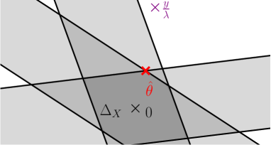
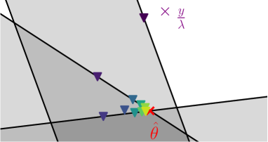
Figure 1: Illustration of the VAR nature of the dual iterates of the Lasso, on a toy dataset with $n=2$ and $p=3$. Left: dual of the Lasso problem; the dual optimum $\hat{\theta}$ is the projection of $y/\lambda$ onto $\Delta_{X}$. Right: sequence of residuals after each update of coordinate descent (first iterates in blue, last in yellow). After four updates, the iterates alternate geometrically between the same two constraint hyperplanes.

Figure 1 represents the Lasso dual for a toy problem and illustrates the VAR nature of $r^{(t)}/\lambda$. As highlighted in Tibshirani (2017), the iterates $r^{(t)}/\lambda$ correspond to the iterates of Dykstra’s algorithm to project $y/\lambda$ onto $\Delta_{X}$. During the first updates, the dual iterates do not have a regular trajectory. However, after a certain number of updates (corresponding to sign identification), they alternate in a geometric fashion between two hyperplanes. In this regime, it becomes beneficial to use extrapolation to obtain a point closer to $\hat{\theta}$.

Remark 11.

Equation 30 shows why we combine extrapolation with cyclic coordinate descent: if the coefficients are not always updated in the same order (see Massias et al. 2018, Figure 1(c-d)), the matrix $A$ depends on the epoch, and the VAR structure may no longer hold.

Having highlighted the VAR behavior of $(X\beta^{(t)})_{t\in\mathbb{N}}$, we can introduce our proposed dual extrapolation.

Definition 12 (Extrapolated dual point for the Lasso).

For a fixed number $K$ of proximal gradient descent or coordinate descent epochs, let $r^{(t)}$ denote the residuals $y-X\beta^{(t)}$ at epoch $t$ of the algorithm. We define the extrapolated residuals

$$r_{\mathrm{acc}}^{(t)}=\begin{cases}r^{(t)},&\mbox{if }t\leq K\enspace,\\ \displaystyle\sum_{k=1}^{K}c_{k}r^{(t+1-k)},&\mbox{if }t>K\enspace.\end{cases}$$ (35)

where $c=(c_{1},\dots,c_{K})^{\top}\in\mathbb{R}^{K}$ is defined as in (16) with $U^{(t)}=[r^{(t+1-K)}-r^{(t-K)},\ldots,r^{(t)}-r^{(t-1)}]\in\mathbb{R}^{n\times K}$. Then, we define the extrapolated dual point as:

$$\theta_{\mathrm{acc}}^{(t)}\stackrel{{\scriptstyle\mbox{\tiny def.}}}{{=}}r_{\mathrm{acc}}^{(t)}/\max(\lambda,\lVert{X^{\top}r_{\mathrm{acc}}^{(t)}}\rVert_{\infty})\enspace.$$ (36)

In practice, we use $K=5$ and do not compute $\theta_{\mathrm{acc}}^{(t)}$ if $U^{(t)}{}^{\top}U^{(t)}$ cannot be inverted. Additionally, to impose monotonicity of the dual objective, and guarantee a behavior at least as good at $\theta_{\mathrm{res}}$, we use as dual point at iteration $t$:

$$\theta^{(t)}=\displaystyle\mathop{\mathrm{arg\,max}}_{\theta\in\{\theta^{(t-1)},\theta_{\mathrm{acc}}^{(t)},\theta_{\mathrm{res}}^{(t)}\}}\mathcal{D}(\theta)\enspace.$$ (37)

There are two reasons why the results of Proposition 6 cannot be straightforwardly applied to Equation 36:

1. the analysis by Scieur et al. (2016) requires $A$ to be symmetrical, which is the case for proximal gradient descent but not for cyclic coordinate descent (as $\operatorname{Id}_{n}-x_{j_{s}}x_{j_{s}}^{\top}/\lVert{x_{j_{s}}}\rVert^{2}$ and $\operatorname{Id}_{n}-x_{j_{s^{\prime}}}x_{j_{s^{\prime}}}^{\top}/\lVert{x_{j_{s^{\prime}}}}\rVert^{2}$ only commute if $x_{j_{s}}$ and $x_{j_{s^{\prime}}}$ are collinear). To circumvent this issue, we can make $A$ symmetrical: instead of considering cyclic updates, we could consider that iterates $\beta^{(t)}$ are produced by a cyclic pass over the coordinates, followed by a cyclic pass over the coordinates in reverse order. The matrix of the VAR in this case is no longer $A=A_{S}\dots A_{1}$, but $A_{1}\dots A_{S}A_{S}\dots A_{1}=A_{1}^{\top}\dots A_{S}^{\top}A_{S}\dots A_{1}=A^{\top}A$ (the $A_{s}$’s are symmetrical). Experiments of Section 6, where a simple cyclic order is used, tend to indicate that there is in fact no need for $A$ to be symmetrical.

2. for both proximal gradient and coordinate descent we have $\left\lVert{A}\right\rVert=1$ instead of $\left\lVert{A}\right\rVert<1$ as soon as $S<n$: if the support of $\hat{\beta}$ is of size smaller than $n$ ($S<n$), 1 is an eigenvalue of $A$. Indeed, for coordinate descent, if $S<n$, there exists a vector $u\in\mathbb{R}^{n}$, orthogonal to the $S$ vectors $x_{j_{1}},\dots,x_{j_{S}}$. The matrix $A_{s}=\operatorname{Id}_{n}-\frac{1}{\lVert{x_{j_{s}}}\rVert^{2}}x_{j_{s}}x_{j_{s}}^{\top}$ being the orthogonal projection onto $\operatorname{Span}(x_{j_{s}})^{\bot}$, we therefore have $A_{s}u=u$ for every $s\in[S]$, hence $Au=u$. For proximal gradient descent, $\tfrac{1}{L}\tilde{X_{S}}\tilde{X_{S}}^{\top}$ is not invertible when $S<n$, hence 1 is an eigenvalue of $\operatorname{Id}_{n}-\tfrac{1}{L}\tilde{X_{S}}\tilde{X_{S}}^{\top}$. This seems to contradict the convergence of the VAR sequence but is addressed in Lemmas 13 and 14.

Lemma 13.

For coordinate descent, if an eigenvalue of $A=A_{S}\dots A_{1}$ has modulus 1, it is equal to 1.

Proof  The matrix $A_{s}=\operatorname{Id}_{n}-\frac{1}{\lVert{x_{j_{s}}}\rVert^{2}}x_{j_{s}}x_{j_{s}}^{\top}$ is the orthogonal projection onto $\operatorname{Span}(x_{j_{s}})^{\bot}$. Hence,

$$\forall x\in\mathbb{R}^{n},\left\lVert{A_{s}x}\right\rVert=\left\lVert{x}\right\rVert\implies A_{s}x=x\enspace.$$ (38)

Let $(\mu,x)\in\mathbb{C}\times\mathbb{R}^{n}$ s.t. $\left\lvert\mu\right\rvert=1$, $\left\lVert{x}\right\rVert=1$ and $Ax=\mu x$. This means $\left\lVert{Ax}\right\rVert=1$. Because $\left\lVert{A_{1}x}\right\rVert<1\implies\left\lVert{A_{S}\dots A_{1}x}\right\rVert\leq\left\lVert{A_{S}\dots A_{2}}\right\rVert\lVert{A_{1}x}\rVert<1\implies\left\lVert{Ax}\right\rVert<1$, we must have $\left\lVert{A_{1}x}\right\rVert\geq 1$. Since it holds that $\left\lVert{A_{1}x}\right\rVert\leq\left\lVert{x}\right\rVert=1$, we have $\left\lVert{A_{1}x}\right\rVert=\left\lVert{x}\right\rVert$, thus $A_{1}x=x$ because $A_{1}$ is an orthogonal projection. By a similar reasoning, $A_{2}x=x$, etc. up to $A_{S}x=x$, hence $Ax=x$ and $\mu=1$.  

Lemma 14.

For coordinate descent (resp. proximal gradient descent) applied to solve the Lasso, the VAR parameters $A\in\mathbb{R}^{n\times n}$ and $b\in\mathbb{R}^{n}$ defined in (30) (resp. (34)) satisfy $b\in\operatorname{Ker}(\operatorname{Id}_{n}-A)^{\perp}$.

Proof 

Coordinate descent case:

Let us remind that $b=A_{S}\dots A_{2}b_{1}+\dots+A_{S}b_{S-1}+b_{S}$ in this case, with $b_{s}=x_{j_{s}}^{\top}y-\lambda\operatorname{sign}(\hat{\beta}_{j_{s}})x_{j_{s}}/\lVert{x_{j_{s}}}\rVert^{2}$. Let $v\in\operatorname{Ker}(\operatorname{Id}_{n}-A)$. Following the proof of Lemma 13, we have $A_{1}v=\dots=A_{S}v=v$. For $s\in[S]$, since $A_{s}$ is the projection on $\operatorname{Span}(x_{j_{s}})^{\bot}$, this means that $v$ is orthogonal to $x_{j_{s}}$. Additionally, $v^{\top}A_{S}\dots A_{s+1}b_{s}=(A_{s+1}\dots A_{S}v)^{\top}b_{s}=v^{\top}b_{s}=0$ since $b_{s}$ is co-linear to $x_{j_{s}}$. Thus, $v$ is orthogonal to the $S$ terms which compose $b$, and $b\perp\operatorname{Ker}(\operatorname{Id}_{n}-A)$.

Proximal gradient descent case:

Let $v\in\operatorname{Ker}(\operatorname{Id}_{n}-A)=\operatorname{Ker}(X_{\mathcal{S}}X_{\mathcal{S}}^{\top})$. We have $v^{\top}X_{\mathcal{S}}X_{\mathcal{S}}^{\top}v=0=\left\lVert{X_{\mathcal{S}}^{\top}v}\right\rVert^{2}$, hence $X_{\mathcal{S}}^{\top}v=0.$ It is now clear that $v^{\top}b=v^{\top}(-X_{\mathcal{S}}X_{\mathcal{S}}^{\top}y+\lambda X_{\mathcal{S}}\operatorname{sign}\hat{\beta})/L=0$, hence $b\perp\operatorname{Ker}(\operatorname{Id}_{n}-A)$.  

Proposition 15.

Proposition 6 holds for the residuals $r^{(t)}$ (produced either by proximal gradient descent or coordinate descent) even though $\lVert{A}\rVert_{2}=1$ in both cases.

Proof  Let us write $A=\bar{A}+\underline{A}$ with $\bar{A}$ the orthogonal projection on $\operatorname{Ker}(\operatorname{Id}_{n}-A)$. By Lemma 13, $\lVert{\underline{A}}\rVert<1$.

Then, one can check that $A\underline{A}=\underline{A}^{2}$ and $A\bar{A}=\bar{A}^{2}=\bar{A}$ and $Ab=\underline{A}b$.

Let $T$ be the epoch when support identification is achieved. For $t\geq T$, we have

$$r^{(t+1)}=\underline{A}r^{(t)}+b+\bar{A}r^{(T)}\enspace.$$ (39)

Indeed, it is trivially true for $t=T$ and if it holds for $t$,

$$r^{(t+2)} =Ar^{(t+1)}+b$$

$$=A(\underline{A}r^{(t)}+b+\bar{A}r^{(T)})+b$$

$$=\underline{A}^{2}r^{(t)}+\underline{A}b+\bar{A}r^{(T)}+b$$

$$=\underline{A}(\underline{A}r^{(t)}+b)+\bar{A}r^{(T)}+b$$

$$=\underline{A}r^{(t+1)}+\bar{A}r^{(T)}+b\enspace.$$ (40)

Therefore, on the space $\operatorname{Ker}(\operatorname{Id}_{n}-A)$, the sequence $r^{(t)}$ is constant, and on its orthogonal $\operatorname{Ker}(\operatorname{Id}_{n}-A)^{\perp}$, it is a VAR sequence with associated matrix $\underline{A}$, whose spectral normal is strictly less than 1. Therefore, the results of Proposition 6 still hold.  

Remark 16 (Connection with primal-dual techniques).

The goal of our construction is to improve convergence for the primal, by constructing a better dual certificate which provides a tighter stopping criterion. In our scheme, the primal iterates directly influence the dual ones – either through the link equation (residuals rescaling), either through extrapolation – but (apart from the influence of screening or working set selection), the primal iterates do not depend on the dual ones. An alternative technique to improve convergence in the dual would be to solve simultaneously the primal and the dual. The objective function in (0) is $F(X\beta)+\lambda\lVert{\beta}\rVert_{1}$, hence since strong duality holds, an equivalent saddle point formulation is

$$\max_{\theta\in\mathbb{R}^{n}}\min_{\beta\in\mathbb{R}^{p},z\in\mathbb{R}^{n}}F(z)+\lambda\lVert{\beta}\rVert_{1}+\lambda\theta^{\top}(z-X\beta)\enspace,\quad\text{{\em i.e.,~{}}}$$ (40)

$$\max_{\theta\in\mathbb{R}^{n}}\min_{\beta\in\mathbb{R}^{p}}\underbrace{-F^{*}(-\lambda\theta)+\lambda\lVert{\beta}\rVert_{1}-\lambda\theta^{\top}X\beta}_{\mathcal{L}(\beta,\theta)}\enspace.$$

To solve this problem, the primal-dual Arrow-Hurwicz (Arrow et al., 1958) method alternates proximal maximization steps in $\theta$ and proximal minimization steps in $\beta$. Here, the maximization step can even be performed exactly, yielding:

$$\begin{cases}\beta^{(t+1)}=\operatorname{prox}_{\lambda/L\lVert{\cdot}\rVert_{1}}(\beta^{(t)}+\frac{\lambda}{L}X^{\top}\theta^{(t)})\enspace,\\ \lambda\nabla F^{*}(-\lambda\theta^{(t+1)})-\lambda X\beta^{(t+1)}=0\enspace,\end{cases}$$ (41)

and the last line is equivalent to $\theta^{(t+1)}=-\nabla F(X\beta^{(t+1)})/\lambda$ (Hiriart-Urruty and Lemaréchal, 1993, Cor. 1.4.4), as in Equation 1. Using inertial variants of the scheme (41), such as the one by Chambolle and Pock (2011) is a potential lead, which we do not investigate further. In our opinion, a more promising direction of research would be to design extrapolation methods for the primal-dual coordinate descent method of Fercoq and Bianchi (2015), which is left to future work. Finally, we are not aware of algorithms working directly in the dual; a reason for that is that getting feasible iterates by other means than rescaling requires the knowledge of the projection onto $\Delta_{X}$, which is as difficult as the primal (see Tibshirani (2017) on this matter). Dünner et al. (2016) use a so-called “Lipschitzing trick” to make the dual unconstrained, but the rough bound $\lambda\lVert{\hat{\beta}}\rVert_{1}\leq F(\mathbf{0}_{n})$ they used is likely to lead to poor values of convergence rate constants in practice.

Although so far we have proven results for both coordinate descent and proximal gradient descent for the sake of generality, we observed that coordinate descent consistently converges faster. Hence from now on, we only consider the latter.

4 Generalized linear models

4.1 Coordinate descent for $\ell_{1}$ regularization

Proposition 17 (VAR for coordinate descent and Sparse GLM).

When (0) is solved by cyclic coordinate descent, the dual iterates $(X\beta^{(t)})_{t\in\mathbb{N}}$ form an asymptotical VAR sequence.

Proof  As in the proof of Proposition 10, we place ourselves in the identified sign regime, and consider only one epoch $t$ of CD: let $\tilde{\beta}^{(0)}$ denote the value of the primal iterate at the beginning of the epoch ($\tilde{\beta}^{(0)}=\beta^{(t)}$), and for $s\in[S]$, $\tilde{\beta}^{(s)}\in\mathbb{R}^{p}$ denotes its value after the $j_{s}$ coordinate has been updated ($\tilde{\beta}^{(S)}=\beta^{(t+1)}$). Recall that in the framework of (0), the data-fitting functions $f_{i}$ have $1/\gamma$-Lipschitz gradients, and ${\nabla F(u)=(f_{1}^{\prime}(u_{1}),\dots,f_{n}^{\prime}(u_{n}))}$.

For $s\in[S]$, $\tilde{\beta}^{(s)}$ and $\tilde{\beta}^{(s-1)}$ are equal everywhere except at entry $j_{s}$, for which the coordinate descent update with fixed step size $\tfrac{\gamma}{\lVert{x_{j_{s}}}\rVert^{2}}$ is

$$\tilde{\beta}^{(s)}_{j_{s}} =\operatorname{ST}\Big{(}\tilde{\beta}^{(s-1)}_{j_{s}}-\tfrac{\gamma}{\lVert{x_{j_{s}}}\rVert^{2}}x_{j_{s}}^{\top}\nabla F(X\tilde{\beta}^{(s-1)}),\tfrac{\gamma}{\lVert{x_{j_{s}}}\rVert^{2}}\lambda\Big{)}$$

$$=\tilde{\beta}^{(s-1)}_{j_{s}}-\tfrac{\gamma}{\lVert{x_{j_{s}}}\rVert^{2}}x_{j_{s}}^{\top}\nabla F(X\tilde{\beta}^{(s-1)})-\tfrac{\gamma}{\lVert{x_{j_{s}}}\rVert^{2}}\lambda\operatorname{sign}(\hat{\beta}_{j_{s}})\enspace.$$ (42)

Therefore,

$$X\tilde{\beta}^{(s)}-X\tilde{\beta}^{(s-1)} =x_{j_{s}}\left(\tilde{\beta}^{(s)}_{j_{s}}-\tilde{\beta}^{(s-1)}_{j_{s}}\right)$$

$$=x_{j_{s}}\left(-\tfrac{\gamma}{\lVert{x_{j_{s}}}\rVert^{2}}x_{j_{s}}^{\top}\nabla F(X\tilde{\beta}^{(s-1)})-\tfrac{\gamma}{\lVert{x_{j_{s}}}\rVert^{2}}\lambda\operatorname{sign}(\hat{\beta}_{j_{s}})\right)\enspace.$$ (43)

Using point-wise linearization of the function $\nabla F$ around $X\hat{\beta}$, we have:

$$\nabla F(X\beta) =\nabla F(X\hat{\beta})+D(X\beta-X\hat{\beta})+o(X\beta-X\hat{\beta})\enspace,$$ (44)

where $D\stackrel{{\scriptstyle\mbox{\tiny def.}}}{{=}}\operatorname{diag}(f_{1}^{\prime\prime}(\hat{\beta}^{\top}\mathbf{x}_{1}),\dots,f_{n}^{\prime\prime}(\hat{\beta}^{\top}\mathbf{x}_{n}))\in\mathbb{R}^{n\times n}$. Therefore

$$X\tilde{\beta}^{(s)} =\left(\operatorname{Id}_{n}-\tfrac{\gamma}{\lVert{x_{j_{s}}}\rVert^{2}}x_{j_{s}}x_{j_{s}}^{\top}D\right)X\tilde{\beta}^{(s-1)}$$

$$\phantom{=}+\tfrac{\gamma}{\lVert{x_{j_{s}}}\rVert^{2}}\left(x_{j_{s}}^{\top}(DX\hat{\beta}-\nabla F(X\hat{\beta}))-\lambda\operatorname{sign}(\hat{\beta}_{j_{s}})\right)x_{j_{s}}+o(X\tilde{\beta}^{(s)}-X\hat{\beta})\enspace,$$

$$D^{1/2}X\tilde{\beta}^{(s)} =\underbrace{\left(\operatorname{Id}_{n}-\tfrac{\gamma}{\lVert{x_{j_{s}}}\rVert^{2}}D^{1/2}x_{j_{s}}x_{j_{s}}^{\top}D^{1/2}\right)}_{A_{s}}D^{1/2}X\tilde{\beta}^{(s-1)}$$

$$\phantom{=\quad}+{\underbrace{\tfrac{\gamma}{\lVert{x_{j_{s}}}\rVert^{2}}x_{j_{s}}^{\top}(DX\hat{\beta})D^{1/2}x_{j_{s}}}_{b_{s}}}+o(X\tilde{\beta}^{(s)}-X\hat{\beta})\enspace,$$ (45)

since the subdifferential inclusion (2) gives $-x_{j_{s}}^{\top}\nabla F(X\hat{\beta})-\lambda\operatorname{sign}(\hat{\beta}_{j_{s}})=0$. Thus, the sequence $(D^{1/2}X\beta^{(t)})_{t\in\mathbb{N}}$ is an asymptotical VAR sequence:

$$D^{1/2}X\beta^{(t+1)}=A_{S}\dots A_{1}D^{1/2}X\beta^{(t)}+b_{S}+\ldots+A_{S}\ldots A_{2}b_{1}+o(X\beta^{(t)}-X\hat{\beta})\enspace,$$ (46)

and so is $(X\beta^{(t)})_{t\in\mathbb{N}}$:

$$X\beta^{(t+1)}=\underbrace{D^{-\tfrac{1}{2}}A_{S}\dots A_{1}D^{\tfrac{1}{2}}}_{A}X\beta^{(t)}+\underbrace{D^{-\tfrac{1}{2}}(b_{S}+\ldots+A_{S}\ldots A_{2}b_{1})}_{b}+o(X\beta^{(t)}-X\hat{\beta})\enspace.$$ (47)

 

Proposition 18.

As in Lemmas 13 and 14, for the VAR parameters $A$ and $b$ defined in Equation 47, 1 is the only eigenvalue of $A$ whose modulus is 1 and $b\perp\operatorname{Ker}(\operatorname{Id}_{n}-A)$.

Proof  First, notice that as in the Lasso case, we have $\operatorname{Id}_{n}\succeq A_{s}\succeq 0$. Indeed, because $f^{\prime\prime}_{i}$ takes values in $]0,1/\gamma[$, $D^{1/2}$ exists and $\tfrac{1}{\sqrt{\gamma}}\operatorname{Id}_{n}\succeq D^{1/2}\succeq 0$. For any $u\in\mathbb{R}^{n}$,

$$u^{\top}D^{1/2}x_{j_{s}}x_{j_{s}}^{\top}D^{1/2}u =(x_{j_{s}}^{\top}D^{1/2}u)^{2}\geq 0,$$ (48)

$$\mbox{and }\quad\quad\quad\quad x_{j_{s}}^{\top}D^{1/2}u \leq\lVert{x_{j_{s}}}\rVert\lVert{D^{1/2}u}\rVert$$

$$\leq\lVert{x_{j_{s}}}\rVert\lVert{D^{1/2}}\rVert\lVert{u}\rVert$$

$$\leq\tfrac{1}{\sqrt{\gamma}}\lVert{x_{j_{s}}}\rVert\lVert{u}\rVert\enspace,$$ (49)

thus $\tfrac{\lVert{x_{j_{s}}}\rVert^{2}}{\gamma}\operatorname{Id}_{n}\succeq D^{1/2}x_{j_{s}}x_{j_{s}}^{\top}D^{1/2}\succeq 0$ and $\operatorname{Id}_{n}\succeq A_{s}\succeq 0$.

However, contrary to the Lasso case, because $\left\lVert{D^{1/2}x_{j_{s}}}\right\rVert\neq\sqrt{\gamma}\left\lVert{x_{j_{s}}}\right\rVert$, $A_{s}$ is not the orthogonal projection on $(\operatorname{Span}D^{1/2}x_{j_{s}})^{\perp}$. Nevertheless, we still have $A_{s}=A_{s}^{\top}$, $\lVert{A_{s}}\rVert\leq 1$, and for $v\in\mathbb{R}^{n}$, $A_{s}v=v$ means that $v^{\top}D^{1/2}x_{j_{s}}=0$, so the proof of Lemma 13 can be applied to show that the only eigenvalue of $A_{S}\ldots A_{1}$ which has modulus 1 is 1. Then, observing that $A=D^{-1/2}A_{S}\dots A_{1}D^{1/2}$ has the same spectrum as $A_{S}\dots A_{1}$ concludes the first part of the proof.

For the second result, let $v\in\operatorname{Ker}(\operatorname{Id}_{n}-A)$, i.e., $Av=v$, hence $A_{S}\ldots A_{1}D^{1/2}v=D^{1/2}Av=D^{1/2}v$. Therefore $D^{1/2}v$ is a fixed point of $A_{S}\ldots A_{1}$, and as in the Lasso case this means that for all $s\in[S]$, $A_{s}D^{1/2}v=D^{1/2}v$ and $(D^{1/2}v)^{\top}D^{1/2}x_{j_{s}}=0$. Now recall that

$$b =D^{-1/2}(b_{S}+\ldots+A_{S}\ldots A_{2}b_{1})\enspace,$$ (50)

$$b_{s} =\tfrac{\gamma}{\lVert{x_{j_{s}}}\rVert^{2}}\left(x_{j_{s}}^{\top}(DX\hat{\beta}-\nabla F(X\hat{\beta}))-\lambda\operatorname{sign}(\hat{\beta}_{j_{s}})\right)D^{1/2}x_{j_{s}}$$

$$=\tfrac{\gamma}{\lVert{x_{j_{s}}}\rVert^{2}}(x_{j_{s}}^{\top}DX\hat{\beta})D^{1/2}x_{j_{s}}\enspace.$$ (51)

Additionally, $v^{\top}D^{-1/2}A_{S}\dots A_{s+1}b_{s}=(A_{s+1}\dots A_{S}D^{-1/2}v)^{\top}b_{s}=(D^{-1/2}v)^{\top}b_{s}=0$. Hence $v$ is orthogonal to all the terms which compose $b$, hence $v^{\top}b=0$.  
Proposition 17 and Proposition 18 show that we can construct an extrapolated dual point for any sparse GLM, by extrapolating the sequence $(r^{(t)}=X\beta^{(t)})_{t\in\mathbb{N}}$ with the construction of Equation 35, and creating a feasible point with:

$$\theta_{\mathrm{acc}}^{(t)}\stackrel{{\scriptstyle\mbox{\tiny def.}}}{{=}}-\nabla F(r_{\mathrm{acc}}^{(t)})/\max(\lambda,\lVert{X^{\top}\nabla F(r_{\mathrm{acc}}^{(t)})}\rVert_{\infty})\enspace.$$ (52)

4.2 Multitask Lasso

Let $q\in\mathbb{N}$ be a number of tasks, and consider an observation matrix $Y\in\mathbb{R}^{n\times q}$, whose $i$-th row is the target in $\mathbb{R}^{q}$ for the $i$-th sample. For $\mathrm{B}\in\mathbb{R}^{p\times q}$, let $\lVert{\mathrm{B}}\rVert_{2,1}=\sum_{1}^{p}\left\lVert{\mathrm{B}_{j}}\right\rVert$ (with $\mathrm{B}_{j}\in\mathbb{R}^{1\times q}$ the $j$-th row of $\mathrm{B}$).

Definition 19.

The multitask Lasso estimator is defined as the solution of:

$$\hat{\mathrm{B}}\in\mathop{\mathrm{arg\,min}}_{\mathrm{B}\in\mathbb{R}^{n\times q}}\frac{1}{2}\left\lVert{Y-X\mathrm{B}}\right\rVert_{F}^{2}+\lambda\left\lVert{\mathrm{B}}\right\rVert_{2,1}\enspace.$$ (53)

Let $j_{1}<\dots<j_{S}$ denote the (row-wise) support of $\hat{\mathrm{B}}$, and let $t$ denote an iteration after support identification. Note that the guarantees of support identification for multitask Lasso requires more assumptions than the case of the standard Lasso. In particular it requires a source condition which depends on the design matrix $X$. This was investigated for instance by Vaiter et al. (2018) when considering a proximal gradient descent algorithm.

Let $\tilde{\mathrm{B}}^{(0)}=\mathrm{B}^{(t)}$, and for $s\in[S]$, let $\tilde{\mathrm{B}}^{(s)}$ denote the primal iterate after coordinate $j_{s}$ has been updated. Let $s\in[S]$, with $\tilde{\mathrm{B}}^{(s)}$ and $\tilde{\mathrm{B}}^{(s-1)}$ being equal everywhere, except for their $j_{s}$ row for which one iteration of proximal block coordinate descent gives, with $\phi(\mathrm{B})\stackrel{{\scriptstyle\mbox{\tiny def.}}}{{=}}\mathrm{B}_{j_{s}}+\frac{1}{\lVert{x_{j_{s}}}\rVert^{2}}x_{j_{s}}^{\top}(Y-X\mathrm{B})\in\mathbb{R}^{1\times q}$:

$$\tilde{\mathrm{B}}^{(s)}_{j_{s}}=\left(1-\frac{\lambda/\left\lVert{x_{j_{s}}}\right\rVert^{2}}{\lVert{\phi(\tilde{\mathrm{B}}^{(s-1)})}\rVert}\right)\phi(\tilde{\mathrm{B}}^{(s-1)})\enspace.$$ (54)

From Equation 54,

$$X\tilde{\mathrm{B}}^{(s)}-X\tilde{\mathrm{B}}^{(s-1)} =x_{j_{s}}(\tilde{\mathrm{B}}^{(s)}_{j_{s}}-\tilde{\mathrm{B}}^{(s-1)}_{j_{s}})$$

$$=x_{j_{s}}\left(\frac{1}{\lVert{x_{j_{s}}}\rVert^{2}}x_{j_{s}}^{\top}(Y-X\tilde{\mathrm{B}}^{(s-1)})-\frac{\lambda/\left\lVert{x_{j_{s}}}\right\rVert^{2}}{\lVert{\phi(\tilde{\mathrm{B}}^{(s-1)})}\rVert}\phi(\tilde{\mathrm{B}}^{(s-1)})\right)\enspace.$$ (55)

Using

$$\frac{x+h}{\lVert{x+h}\rVert} =\frac{x}{\lVert{x}\rVert}+\frac{1}{\lVert{x}\rVert}\Big{(}\operatorname{Id}-\frac{xx^{\top}}{\lVert{x}\rVert^{2}}\Big{)}h+o(\lVert{h}\rVert),$$ (56)

and introducing $\psi\stackrel{{\scriptstyle\mbox{\tiny def.}}}{{=}}e_{j_{s}}^{\top}-\frac{1}{\lVert{x_{j_{s}}}\rVert^{2}}x_{j_{s}}^{\top}X\in\mathbb{R}^{1\times p}$, so that $\phi(\mathrm{B})=\phi(\hat{\mathrm{B}})+\psi(\mathrm{B}-\hat{\mathrm{B}})$, one has the following linearization:

$$\frac{\phi(\mathrm{B})}{\lVert{\phi(\mathrm{B})}\rVert} =\frac{\phi(\hat{\mathrm{B}})}{\lVert{\phi(\hat{\mathrm{B}})}\rVert}+\frac{1}{\lVert{\phi(\hat{\mathrm{B}})}\rVert}\psi(\mathrm{B}-\hat{\mathrm{B}})\left(\operatorname{Id}_{q}-\frac{\phi(\hat{\mathrm{B}})^{\top}\phi(\hat{\mathrm{B}})}{\lVert{\phi(\hat{\mathrm{B}})}\rVert^{2}}\right)+o(\mathrm{B}-\hat{\mathrm{B}})\enspace,$$ (57)

which does not allow to exhibit a VAR structure, as $\mathrm{B}$ should appear only on the right. Despite this negative result, empirical results of Section 6 show that dual extrapolation still provides a tighter dual point in the identified support regime. Celer’s generalization to multitask Lasso consists in using $d_{j}^{(t)}=(1-\lVert{x_{j}^{\top}\Theta^{(t)}}\rVert)/{\lVert{x_{j}}\rVert}$ with the dual iterate $\Theta^{(t)}\in\mathbb{R}^{n\times q}$. The inner solver is cyclic block coordinate descent (BCD), and the extrapolation coefficients are obtained by solving Equation 15, which is an easy to solve matrix least-squares problem.

Remark 20.

As a concluding remark, we point that for the three models studied here, a VAR structure in the dual implies a VAR structure in the primal, provided $X_{\mathcal{S}(\hat{\beta})}$ has full column rank. Indeed, for any matrix $B$ such that $BX_{\mathcal{S}(\hat{\beta})}=\operatorname{Id}_{\lVert{\hat{\beta}}\rVert_{0}}$, after support identification one has $\beta^{(t+1)}_{\mathcal{S}(\hat{\beta})}=BAX_{\mathcal{S}(\hat{\beta})}\beta^{(t)}_{\mathcal{S}(\hat{\beta})}+Bb$. This paves the way for applying the techniques introduced here to extrapolation in the primal, which we leave to future work.

5 Working sets

Being able to construct a better dual point leads to a tighter gap and a smaller upper bound in Equation 4, hence to more features being discarded and a greater speed-up for Gap Safe screening rules. As we detail in this section, it can easily be integrated in a efficient working set policy.

5.1 Improved working sets policy

Working set methods originated in the domains of linear and quadratic programming (Thompson et al., 1966; Palacios-Gomez et al., 1982; Myers and Shih, 1988), where they are called active set methods.

In the context of this paper, a working set approach starts by solving (0) restricted to a small set of features $\mathcal{W}^{(0)}\subset[p]$ (the working set), then defines iteratively new working sets $\mathcal{W}^{(t)}$ and solves a sequence of growing problems (Kowalski et al., 2011; Boisbunon et al., 2014; Santis et al., 2016). It is easy to see that when $\mathcal{W}^{(t)}\subsetneq\mathcal{W}^{(t+1)}$ and when the subproblems are solved up to the precision required for the whole problem, then working sets techniques converge.

It was shown by Massias et al. (2017) that every screening rule which writes

$$\forall j\in[p],\quad d_{j}>\tau\Rightarrow\hat{\beta}_{j}=0\enspace,$$ (58)

allows to define a working set policy. For example for Gap Safe rules,

$$d_{j}=d_{j}(\theta)\stackrel{{\scriptstyle\mbox{\tiny def.}}}{{=}}\frac{1-\lvert x_{j}^{\top}\theta\rvert}{\left\lVert{x_{j}}\right\rVert}\enspace,$$ (59)

is defined as a function of a dual point $\theta\in\Delta_{X}$. The value $d_{j}$ can be seen as measuring the importance of feature $j$, and so given an initial size $p^{(1)}$ the first working set can be defined as:

$$\mathcal{W}^{(1)}=\{j_{1}^{(1)},\dots,j_{p^{(1)}}^{(1)}\}\enspace,$$ (60)

with $d_{j_{1}^{(1)}}(\theta)\leq\dots\leq d_{j^{(1)}_{p^{(1)}}}(\theta)<d_{j}(\theta),\,\forall j\notin\mathcal{W}^{(0)}$, i.e., the indices of the $p^{(1)}$ smallest values of $d(\theta)$. Then, the subproblem solver is launched on $X_{\mathcal{W}^{(1)}}$. New primal and dual iterates are returned, which allow to recompute $d_{j}$’s and define iteratively:

$$\mathcal{W}^{(t+1)}=\{j_{1}^{(t+1)},\dots,j_{p^{(t+1)}}^{(t+1)}\}\enspace,$$ (61)

where we impose $d_{j}(\theta)=-1$ when $\beta_{j}^{(t)}\neq 0$ to keep the active features in the next working set. As in Massias et al. (2018), we choose $p^{(t)}=\min(p,2\lVert{\beta^{(t)}}\rVert_{0})$ to ensure a fast initial growth of the working set, and avoid growing too much when the support is nearly identified. The stopping criterion for the inner solver on $\mathcal{W}^{(t)}$ is to reach a gap lower than a fraction $\rho=0.3$ of the duality gap for the whole problem, $\mathcal{P}(\beta^{(t)})-\mathcal{D}(\theta^{(t)})$. These adaptive working set policies are commonly used in practice (Johnson and Guestrin, 2015, 2018).

Combined with coordinate descent as an inner solver, this algorithm was coined Celer (Constraint Elimination for the Lasso with Extrapolated Residuals) when addressing the Lasso problem. The results of Section 4 justify the use of dual extrapolation for any sparse GLM, thus enabling us to generalize Celer to the whole class of models (Algorithm 2).

input : $X,y,\lambda,\beta^{(0)},\theta^{(0)}$

param : $K=5,p^{(1)}=100,\epsilon,\text{{MAX\_WS}}$

init :  $\mathcal{W}^{(0)}=\emptyset$

1if $\beta^{(0)}\neq\mathbb{0}_{p}$ then $p^{(1)}=|\mathcal{S}(\beta^{(0)})|$;

2 // warm start for  $t=1,\ldots,\emph{\text{{MAX\_WS}}}$  do

       compute $\theta_{\mathrm{res}}^{(t)}$ ;

       // Equation 5

3      

4      if solver is Prox-Celer then

5             do $K$ passes of CD on the support of $\beta^{(t)}$, extrapolate to produce $\theta_{\mathrm{acc}}^{(t-1)}$

6            $\theta_{\mathrm{inner}}^{(t-1)}=\mathop{\mathrm{arg\,max}}_{\theta\in\{\theta^{(t-1)},\theta_{\mathrm{inner}}^{(t-1)}\}}\mathcal{D}(\theta)$

7      $\theta^{(t)}=\mathop{\mathrm{arg\,max}}_{\theta\in\{\theta^{(t-1)},\theta_{\mathrm{inner}}^{(t-1)},\theta_{\mathrm{res}}^{(t)}\}}\mathcal{D}(\theta)$

      $g^{(t)}=\mathcal{P}(\beta^{(t-1)})-\mathcal{D}(\theta^{(t)})$;

       // global gap

8       if  $g^{(t)}\leq\epsilon$ then break;

9      

      $\epsilon^{(t)},\mathcal{W}^{(t)}=\texttt{create\_WS()}$ // get tolerance and working set with Algorithm 3

10      

      // Subproblem solver is Algorithm 1 or 4 for Prox-Celer:

11      

12      get ​$\tilde{\beta}^{(t)},\theta_{\mathrm{inner}}^{(t)}$ with subproblem solver applied to $(X_{\mathcal{W}^{(t)}},y,\lambda,(\beta^{(t-1)})_{\mathcal{W}^{(t)}},\epsilon^{(t)})$

13      $\theta_{\mathrm{inner}}^{(t)}=\theta_{\mathrm{inner}}^{(t)}/\max(1,\lVert{X^{\top}\theta_{\mathrm{inner}}^{(t)}}\rVert_{\infty})$

14      set $\beta^{(t)}=\mathbb{0}_{p}$ and $(\beta^{(t)})_{\mathcal{W}^{(t)}}=\tilde{\beta}^{(t)}$

return $\beta^{(t)},\theta^{(t)}$

Algorithm 2 Celer for (0)

input : $X,y,\lambda,\beta^{(t-1)},\theta^{(t)},\mathcal{W}^{(t-1)},g^{(t)}$

param : $p^{(1)}=100,\rho=0.3$

init : $d=\mathbf{0}_{p}$

1

2for $j=1,\ldots,p$ do

3       if  $\beta^{(t-1)}_{j}\neq 0$ then $d_{j}^{(t)}=-1$;

4       else $d_{j}^{(t)}=(1-\lvert x_{j}^{\top}\theta^{(t)}\rvert)/{\lVert{x_{j}}\rVert}$;

5      

6$\epsilon^{(t)}=\rho g^{(t)}$

7if $t\geq 2$ then $p^{(t)}=\min(2\lVert{\beta^{(t-1)}}\rVert_{0},p)$;

8

9$\mathcal{W}^{(t)}=\{j\in[p]\,:\,d^{(t)}_{j}\text{ among }p^{(t)}\text{ smallest values of}\;d^{(t)}\}$

return $\epsilon^{(t)},\mathcal{W}^{(t)}$

Algorithm 3 create_WS

5.2 Newton-Celer

When using a squared $\ell_{2}$ loss, the curvature of the loss is constant: for the Lasso and multitask Lasso, the Hessian does not depend on the current iterate. This is however not true for other GLM data fitting terms, e.g., Logistic regression, for which taking into account the second order information proves to be very useful for fast convergence (Hsieh et al., 2014). To leverage this information, we can use a prox-Newton method (Lee et al., 2012; Scheinberg and Tang, 2013) as inner solver; an advantage of dual extrapolation is that it can be combined with any inner solver, as we detail below. For reproducibility and completeness, we first briefly detail the Prox-Newton procedure used. In the following and in Algorithms 4, 5 and 6 we focus on a single subproblem optimization, so for lighter notation we assume that the design matrix $X$ is already restricted to features in the working set. The reader should be aware that in the rest of this section, $\beta$, $X$ and $p$ in fact refers to $\beta_{\mathcal{W}^{(t)}}$, $X_{\mathcal{W}^{(t)}}$, and $p^{(t)}$.

Writing the data-fitting term $f(\beta)=F(X\beta)$, we have $\nabla^{2}f(\beta)=X^{\top}DX$, where $D\in\mathbb{R}^{n\times n}$ is diagonal with $f_{i}^{\prime\prime}(\beta^{\top}\mathbf{x}_{i})$ as its $i$-th diagonal entry. Using $H=\nabla^{2}f(\beta^{(t)})$ we can approximate the primal objective by

$$f(\beta^{(t)})+\nabla f(\beta^{(t)})^{\top}(\beta-\beta^{(t)})+\frac{1}{2}(\beta-\beta^{(t)})^{\top}H(\beta-\beta^{(t)})+\lambda\left\lVert{\beta}\right\rVert_{1}\enspace.$$ (62)

Minimizing this approximation yields the direction $\Delta^{(t)}$ for the proximal Newton step:

$$\Delta^{(t)}+\beta^{(t)} =\mathop{\mathrm{arg\,min}}_{\beta}\frac{1}{2}\left\lVert{\beta-\beta^{(t)}+H^{-1}\nabla f(\beta^{(t)})}\right\rVert^{2}_{H}+\lambda\left\lVert{\beta}\right\rVert_{1}\enspace.$$ (63)

Then, a step size $\alpha^{(t)}$ is found by backtracking line search (Algorithm 6), and:

$$\beta^{(t+1)}=\beta^{(t)}+\alpha^{(t)}\Delta^{(t)}\enspace.$$ (64)

The approximation in (62) is the sum of a quadratic function and a $\ell_{1}$ penalty, hence it can be minimized with proximal coordinate descent. Since $H=X^{\top}DX$, coordinate descent can be implemented efficiently by keeping the model fit $X\beta$ up-to-date. The algorithm is summarized in Algorithm 5.

input : $X=[x_{1}|\dots|x_{p}]\in\mathbb{R}^{n\times p},y\in\mathbb{R}^{n},\lambda,\beta^{(0)}\in\mathbb{R}^{p},\epsilon$

param : $\text{{MAX\_CD}}=20,\text{{MAX\_BACKTRACK}}=10,K=5$

init : $\Delta\beta=\mathbf{0}_{p},X\Delta\beta=\mathbf{0}_{n},\theta^{(0)}=\mathbf{0}_{n},D=\mathbf{0}_{n\times n},L=\mathbf{0}_{p},$

1for $t=1,\ldots,T$ do

2      

3      for $i=1,\ldots,n$ do  $D_{ii}=f_{i}^{\prime\prime}(\beta^{\top}\mathbf{x}_{i})\left(={\exp(y_{i}\beta^{\top}\mathbf{x}_{i})}/{\left(1+\exp(y_{i}\beta^{\top}\mathbf{x}_{i})\right)^{2}}\right)$ ;

4       for $j=1,\ldots,p$ do  $L_{j}=\langle x_{j},x_{j}\rangle_{D}\left(=\sum_{i=1}^{n}x_{ij}^{2}{\exp(y_{i}\beta^{\top}\mathbf{x}_{i})}/{\left(1+\exp(y_{i}\beta^{\top}\mathbf{x}_{i})\right)^{2}}\right)$ ;

5      

6      if $t=1$ then $\texttt{\text{{MAX\_CD}}}=1$;

7       else $\texttt{\text{{MAX\_CD}}}=20$;

8       $\Delta\beta=\texttt{newton\_direction}(X,y,\beta^{(t-1)},D,L=(L_{1},\dots,L_{p}),\text{{MAX\_CD}})$

9      $\alpha^{(t)}=\texttt{backtracking}(\Delta\beta,X\Delta\beta,y,\lambda,\text{{MAX\_BACKTRACK}})$

10      $\beta^{(t)}=\beta^{(t-1)}+\alpha^{(t)}\times\Delta\beta$

11      $\theta_{\mathrm{res}}^{(t)}=-\nabla F(X\beta^{(t)})/\lambda\left(=-y/(\lambda\mathbf{1}_{n}+\lambda\exp(y\odot X\beta^{(t)}))\right)$

12      $\theta_{\mathrm{res}}^{(t)}=\theta_{\mathrm{res}}^{(t)}/\max(1,\lVert{X^{\top}\theta_{\mathrm{res}}^{(t)}}\rVert_{\infty})$

13      $\theta^{(t)}=\mathop{\mathrm{arg\,max}}_{\theta\in\{\theta^{(t-1)},\theta_{\mathrm{res}}\}}\mathcal{D}(\theta)$ if $\mathcal{P}(\beta^{(t)})-\mathcal{D}(\theta^{(t)})<\epsilon$ then

14            break

return $\beta^{(t)}$, $\theta^{(t)}$

Algorithm 4 Prox-Newton subproblem solver (illustrated on logistic regression)

input : $X=[x_{1}|\dots|x_{p}]\in\mathbb{R}^{n\times p},y\in\mathbb{R}^{n},\beta\in\mathbb{R}^{p},D\in\mathbb{R}^{n\times n},L=(x_{j}^{\top}Dx_{j})_{j}\in\mathbb{R}^{p},\text{{MAX\_CD}}$

param : $\epsilon,\texttt{MIN\_CD}=2$

init : $\Delta\beta=\mathbf{0}_{p},X\Delta\beta=\mathbf{0}_{n}$

1

2for $k=1,\dots,\emph{\text{{MAX\_CD}}}$ do

       $\tau=0$ // stopping condition

3       for $j=1,\dots,p$ do

4            

5            $u_{j}=\beta_{j}+(\Delta\beta)_{j}$

6            $\tilde{u}_{j}=\operatorname{ST}\left(\beta_{j}+(\Delta\beta)_{j}-\frac{1}{L_{j}}\left(x_{j}^{\top}\nabla F(X\beta^{(t)})-x_{j}^{\top}DX\Delta\beta\right),\frac{\lambda}{L_{j}}\right)$

7            $(\Delta\beta)_{j}=\tilde{u}_{j}-\beta_{j}$

8            $X\Delta\beta\mathrel{+}=(\tilde{u}_{j}-u_{j})x_{j}$

9            $\tau\mathrel{+}=(\tilde{u}_{j}-u_{j})^{2}\times L_{j}^{2}$

10      if $\tau\leq\epsilon$ and $k\geq\mathrm{\emph{{MIN\_CD}}}$ then break;

11      

return $\Delta\beta$

Algorithm 5 newton_direction (illustrated on logistic regression)

Contrary to coordinate descent, Newton steps do not lead to an asymptotic VAR, which is required to guarantee the success of dual extrapolation. To address this issue, we compute $K$ passes of cyclic coordinate descent restricted to the support of the current estimate $\beta$ before defining a working set (Algorithm 2, line 2). The $K$ values of $X\beta$ obtained allow for the computation of both $\theta_{\mathrm{acc}}$ and $\theta_{\mathrm{res}}$. The motivation for restricting the coordinate descent to the support of the current estimate $\beta$ comes from the observation that dual extrapolation proves particularly useful once the support is identified.

The Prox-Newton solver we use is detailed in Algorithm 4. When Algorithm 2 is used with Algorithm 4 as inner solver, we refer to it as the Newton-Celer variant.

Values of parameters and implementation details

In practice, Prox-Newton implementations such as GLMNET (Friedman et al., 2010), newGLMNET (Yuan et al., 2012) or QUIC (Hsieh et al., 2014) only solve the direction approximately in Equation 63. How inexactly the problem is solved depends on some heuristic values. For reproducibility, we expose the default values of these parameters as inputs to the algorithms. Importantly, the variable MAX_CD is set to 1 for the computation of the first Prox-Newton direction. Experiments have indeed revealed that a rough Newton direction for the first update was sufficient and resulted in a substantial speed-up. Other parameters are set based on existing Prox-Newton implementations such as Blitz.

input : $\Delta\beta,X\Delta\beta,\lambda$

param : $\text{{MAX\_BACKTRACK}}=20$

init : $\alpha=1$

1for $k=1,\dots,\text{\text{{MAX\_BACKTRACK}}}$ do

2       $\delta=0$

3      for $j=1,\dots,p$ do

4            

5            if $\beta_{j}+\alpha\times(\Delta\beta)_{j}<0$ then $\delta\mathrel{-}=\lambda(\Delta\beta)_{j}$;

6             else if $\beta_{j}+\alpha\times(\Delta\beta)_{j}>0$ then $\delta\mathrel{+}=\lambda(\Delta\beta)_{j}$;

7             else if $\beta_{j}+\alpha\times(\Delta\beta)_{j}=0$ then $\delta\mathrel{-}=\lambda\left\lvert(\Delta\beta)_{j}\right\rvert$;

8            

9      $\theta=\nabla F(X\beta+\alpha\times X\Delta\beta)\left(=-y\odot\sigma(-y\odot(X\beta+\alpha\times X\Delta\beta))\right)$

10      $\delta\mathrel{+}=(X\Delta\beta)^{\top}\theta$

11      if $\delta<0$ then break;

12       else $\alpha=\alpha/2$;

13      

return $\alpha$

Algorithm 6 backtracking (illustrated on logistic regression)

6 Experiments

In this section, we numerically illustrate the benefits of dual extrapolation on various data sets. Implementation is done in Python, Cython (Behnel et al., 2011) and numba (Lam et al., 2015) for the low-level critical parts. The solvers exactly follow the scikit-learn API (Pedregosa et al., 2011; Buitinck et al., 2013), so that Celer can be used as a drop-in replacement in existing code. The package is available under BSD3 license at https://github.com/mathurinm/celer, with documentation and examples at https://mathurinm.github.io/celer.

In all this section, the estimator-specific $\lambda_{\max}$ refers to the smallest value giving a null solution (for instance $\lambda_{\max}=\lVert{X^{\top}y}\rVert_{\infty}$ in the Lasso case, $\lambda_{\max}=\lVert{X^{\top}y}\rVert_{\infty}/2$ for sparse logistic regression, and $\lambda_{\max}=\lVert{X^{\top}Y}\rVert_{2,\infty}$ for the Multitask Lasso).

Table 1: Characteristics of datasets used

name	$n$	$p$	$q$	density
leukemia	$72$	$7129$	-	$1$
news20	$19996$	$632983$	-	$6.1\,10^{-4}$
rcv1_train	$20242$	$19960$	-	$3.7\,10^{-3}$
finance (log1p)	$16087$	$1668738$	-	$3.4\,10^{-3}$
Magnetoencephalography (MEG)	$305$	$7498$	49	$1$

6.1 Illustration of dual extrapolation

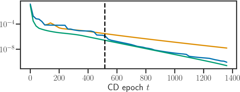
(a) Lasso, on news20 for $\lambda=\lambda_{\max}/5$.

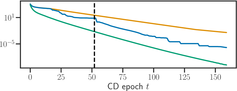
(b) Log. reg., on rcv1 (train) for $\lambda=\lambda_{\max}/20$.

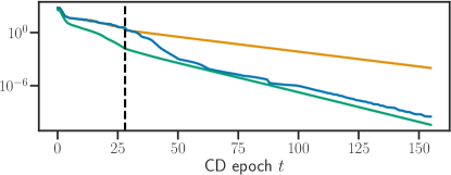
(c) Multitask Lasso, on MEG data for $\lambda=\lambda_{\max}/10$.

Figure 2: Dual objectives with classical and proposed approach, for Lasso (top left), Logistic regression (top right), Multitask Lasso (bottom). The dashed line marks sign identification (support identification for Multitask Lasso).

For the Lasso (Figure 2(a)), Logistic regression (Figure 2(b)) and Multitask Lasso (Figure 2(c)), we illustrate the applicability of dual extrapolation. Monotonicity of the duality gap computed with extrapolation is enforced via the construction of Equation 37. For all problems, the figures show that $\theta_{\mathrm{acc}}$ gives a better dual objective after sign identification, with a duality gap sometimes even matching the suboptimality gap. They also show that the behavior is stable before identification.

In particular, Figure 2(c) hints that dual extrapolation works in practice for the Multitask Lasso, even though there is no such result as sign identification, and we are not able to exhibit a VAR behavior for $(X\mathrm{B}^{(t)})_{t\in\mathbb{N}}$. Figure 1 suggests that the lower the stopping criterion threshold $\epsilon$, the higher the impact of dual extrapolation is. However, when combined with screening, this improvement can be less visible in terms of time: if a large number of variables are screened before support identification, the later iterations concern a very small number of features. In this case, decreasing the duality gap by running the solver longer after screening is not costly.

6.2 Alternative exploitation of VAR structure

Once one postulates that $\hat{\theta}$ is a linear combination of the $K$ most recent residuals, alternatives to our proposed dual extrapolation can be investigated to determine the coefficients of this combination. This is particularly appealing in the Lasso case, for which the dual (0) is:

$$\hat{\theta}=\mathop{\mathrm{arg\,max}}_{\theta\in\Delta_{X}}\;\frac{1}{2}\lVert{y}\rVert^{2}-\frac{\lambda^{2}}{2}\lVert{y/\lambda-\theta}\rVert^{2}\enspace.$$ (64)

In this case, assuming that $\hat{\theta}$ belongs to $\operatorname{Span}(r^{(t)},\ldots,r^{(t-K+1)})$, we can reformulate (64) as a $K$-dimensional quadratic program, and directly optimize over the extrapolation coefficients. If we write $R=[r^{(t)}|\ldots|r^{(t-K+1)}]\in\mathbb{R}^{n\times K}$ and assume that $\hat{\theta}=R\hat{c}$, then (64) is equivalent to:

$$\hat{c} =\mathop{\mathrm{arg\,min}}_{c\in\mathbb{R}^{K}}\;\frac{1}{2}\lVert{y/\lambda-Rc}\rVert^{2}\text{\quad subject to \quad}-\mathbf{1}_{p}\preceq X^{\top}Rc\preceq\mathbf{1}_{p}$$ (64)

$$=\mathop{\mathrm{arg\,min}}_{c\in\mathbb{R}^{K}}\;\frac{\lambda}{2}c^{\top}(R^{\top}R)c-(R^{\top}y)^{\top}c\text{\quad subject to \quad}Ac\preceq\mathbf{1}_{2p}\enspace,$$

where $A^{\top}=[R^{\top}X;-R^{\top}X]^{\top}\in\mathbb{R}^{2p\times K}$. (64) can be solved straightforwardly with solvers such as CVXPY (Diamond and Boyd, 2016), which we use in Figure 3. As visible on the latter, the QP approach seems to suffer more from numerical instabilities: at some iterations, CVXPY does not converge, which we represent by setting the dual objective to 0, hence the visible peaks. Although it performs similarly to dual extrapolation at first, the QP dual point appears to eventually perform the same as residuals rescaling. We do not perform an extensive time study of the compared approaches, but have observed that the $2p$ constraints of (64) make it orders of magnitude slower to solve. In practice, we therefore had to limit the experiment to the rather small leukemia dataset to get reasonable running times. Finally, the QP approach does not lead to simple optimization problems for sparse logistic regression and Multitask Lasso.

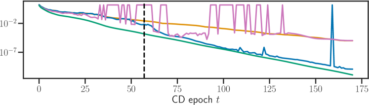
Figure 3: Duality gaps evaluated with rescaled residuals (yellow), our proposed dual extrapolation (blue), QP approach (purple) and optimal dual point (green), on the leukemia dataset, with $\lambda=\lambda_{\max}/5$ resulting in 23 non-zero coefficients at optimum. The dashed line marks support identification. Peaks occur because we set the duality gap to 0 when a method numerically fails to produce extrapolation coefficients.

6.3 Improved screening and working set policy

In order to have a stopping criterion scaling with $n$, the solvers are stopped when the duality gap goes below $\epsilon\times F(\mathbf{0}_{n})$. Features are normalized to have norm 1, and for sparse datasets, features with strictly less than 4 non-zero entries are removed.

6.3.1 Lasso

Path computation

For a fine (resp. coarse) grid of 100 (resp. 10) values of $\lambda$ geometrically distributed between $\lambda_{\max}$ and $\lambda_{\max}/100$, the competing algorithms solve the Lasso on various real world datasets from LIBSVM (Fan et al., 2008). Warm start is used for all algorithms: except for the first value of $\lambda$, the algorithms are initialized with the solution obtained for the previous value of $\lambda$ on the path. Note that paths are computed following a decreasing sequence of $\lambda$ (from high value to low). Computing Lasso solutions for various values of $\lambda$ is a classical task, in cross-validation for example. The values we choose for the grid are the default ones in scikit-learn or GLMNET. For Gap Safe Rules (GSR), we use the strong warm start variant which was shown by Ndiaye et al. (2017, Section 4.6.4) to have the best performance. We refer to “GSR + extr.” when, on top of this, our proposed dual extrapolation technique is used to create the dual points for screening. To evaluate separately the performance of working sets and extrapolation, we also implement “Celer w/o extr.”, i.e., Algorithm 2 without using extrapolated dual point. Doing this, GSR can be compared to GSR + extrapolation, and Celer without extrapolation to Celer. Finally, we also add the performance of Blitz (Johnson and Guestrin, 2018) and StingyCD (Johnson and Guestrin, 2017), the latter being a Lasso-specific coordinate descent designed to skip zero-to-zero updates. Note that dual extrapolation could easily be combined with the update policy of StingyCD. For fair comparison, all algorithms use the duality gap as a stopping criterion.

On Figures 4, 5 and 6, one can see that using acceleration systematically improves the performance of Gap Safe rules, up to a factor 3. Similarly, dual extrapolation makes Celer more efficient than a WS approach without extrapolation (Blitz or Celer w/o extr.) This improvement is more visible for low values of stopping criterion $\epsilon$, as dual extrapolation is beneficial once the support is identified. Generally, working set approaches tend to perform better on coarse grid, while screening is beneficial on fine grids – a finding corroborating Lasso experiments in Ndiaye et al. (2017, Sec. 6.1). Indeed, on a fine grid, the value of the regularizer $\lambda$ changes slowly and each solution on the grid is close to the previous one. In this case, when warm-start is used, the initialization (approximate solution for the previous value of the regularizer) is close to the solution for the new value of the regularizer, and the duality gap always remains low, allowing to quickly screen features. On the contrary, if the grid is coarse, each problem on the grid is quite different from the previous one. Warm start here provides a less useful initialization as the duality gap is higher for the early iterations of each problem. This results in a reduced efficiency of screening.

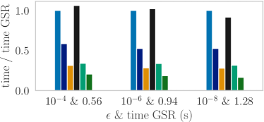
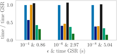
Figure 4: Time to compute a Lasso path from $\lambda_{\max}$ to $\lambda_{\max}/100$ on the leukemia dataset (left: coarse grid of 10 values, right: fine grid of 100 values). $\lambda_{\max}/100$ gives a solution with $60$ nonzero coefficients.

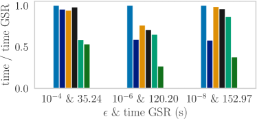
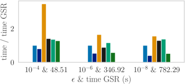
Figure 5: Time to compute a Lasso path from $\lambda_{\max}$ to $\lambda_{\max}/100$ on the news20 dataset (left: coarse grid of 10 values, right: fine grid of 100 values). $\lambda_{\max}/100$ gives a solution with $14817$ nonzero coefficients.

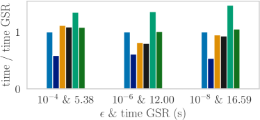
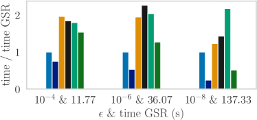
Figure 6: Time to compute a Lasso path from $\lambda_{\max}$ to $\lambda_{\max}/100$ on the rcv1 dataset (left: coarse grid of 10 values, right: fine grid of 100 values). $\lambda_{\max}/100$ gives a solution with $4610$ nonzero coefficients.

Single $\lambda$

Table 2: Computation time (in seconds) for Celer, Blitz and scikit-learn to reach a given precision $\epsilon$ on the Finance dataset with $\lambda=\lambda_{\max}/20$ (without warm start: $\beta^{(0)}=\mathbb{0}_{p}$).

$\epsilon$	$10^{-2}$	$10^{-3}$	$10^{-4}$	$10^{-6}$
Celer	$5$	$7$	$8$	$10$
Blitz	$25$	$26$	$27$	$30$
scikit-learn	$470$	$1350$	$2390$	-

The performance observed in the previous paragraph is not only due to the sequential setting: in the experiment of Table 2, we solve the Lasso for a single value of $\lambda=\lambda_{\max}/20$. The duality gap stopping criterion $\epsilon$ varies between $10^{-2}$ and $10^{-6}$. Celer is orders of magnitude faster than scikit-learn, which uses vanilla CD. The working set approach of Blitz is also outperformed, especially for low $\epsilon$ values.

6.3.2 Logistic regression

In this section, we evaluate separately the first order solvers (Gap Safe, Gap Safe with extrapolation, Celer with coordinate descent as inner solver), and the Prox-Newton solvers: Blitz, Newton-Celer with working set but without using dual extrapolation (PN WS), and Newton-Celer.

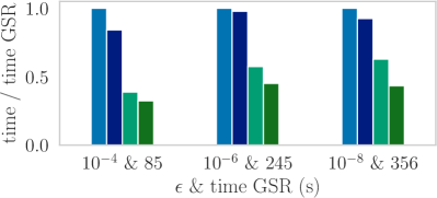
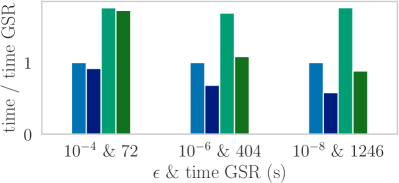
Figure 7: Time to compute a Logistic regression path from $\lambda_{\max}$ to $\lambda_{\max}/100$ on the news20 dataset (left: coarse grid of 10 values, right: fine grid of 100 values). $\lambda_{\max}/100$ gives 5319 non-zero coefficients.

Figure 7 shows that when cyclic coordinate descent is used, extrapolation improves the performance of screening rules, and that using a dual-based working set policy further reduces the computational burden.

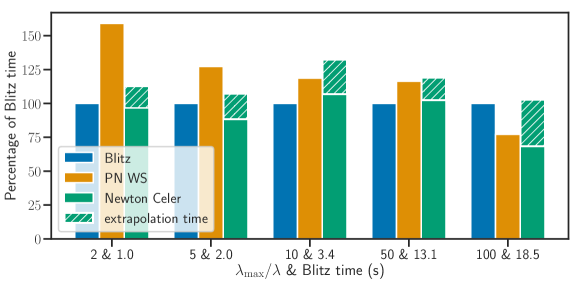
Figure 8: Time to solve a Logistic regression problem for different values of $\lambda$, on the rcv1 dataset ($\epsilon=10^{-6}$).

Figure 8 shows the limitation of dual extrapolation when second order information is taken into account with a Prox-Newton: because the Prox-Newton iterations do not create a VAR sequence, it is necessary to perform some passes of coordinate descent to create $\theta_{\mathrm{acc}}$, as detailed in Section 5.2. This particular experiment reveals that this additional time unfortunately mitigates the gains observed in better working sets and stopping criterion.

6.3.3 Multitask Lasso

The data for this experiment uses magnetoencephalography (MEG) recordings which are collected for neuroscience studies. Here we use data from the sample dataset of the MNE software (Gramfort et al., 2014). Data were obtained using auditory stimulation. There are $n=305$ sensors, $p=$7498$$ source locations in the brain, and the measurements are time series of length $q=49$. Using a Multitask Lasso formulation allows to reconstruct brain activitiy exhibiting a stable sparsity pattern across time (Gramfort et al., 2012). The inner solver for Celer is block coordinate descent, which is also used for the Gap Safe solver (Ndiaye et al., 2015).

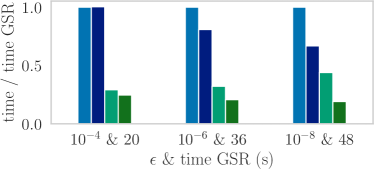
Figure 9: Time to compute a Multitask Lasso path from $\lambda_{\max}$ to $\lambda_{\max}/100$ on MEG data (left: coarse grid of 10 values, right: fine grid of 100 values). $\lambda_{\max}/100$ gives $254$ non-zero rows for $\hat{\mathrm{B}}$.

While Figure 2(c) showed that for the Multitask Lasso the dual extrapolation performance also gives an improved duality gap, here Figure 9 shows that the working set policy of Celer performs better than Gap Safes rules with strong active warm start. We could not include Blitz in the benchmark as there is no standard public implementation for this problem.

Conclusion

In this work, we generalize the dual extrapolation procedure for the Lasso (Celer) to a wider class of $\ell_{1}$-penalized problems, in particular sparse Logistic regression. Theoretical guarantees based on sign identification of coordinate descent are provided. Experiments show that dual extrapolation yields more efficient Gap Safe screening rules and working sets solver. Finally, we adapt Celer to make it compatible with prox-Newton solvers, and empirically demonstrate its applicability to the Multi-task Lasso, for which we leave the proof to future work.

Acknowledgments

This work was funded by the ERC Starting Grant SLAB ERC-StG-676943, by the Chair Machine Learning for Big Data at Télécom ParisTech and by the ANR grant GraVa ANR-18-CE40-0005.

References

- Arrow et al. (1958) K. Arrow, L. Hurwicz, and H. Uzawa. Studies in Nonlinear Programming. Stanford University Press, 1958.
- Bach et al. (2012) F. Bach, R. Jenatton, J. Mairal, and G. Obozinski. Convex optimization with sparsity-inducing norms. Foundations and Trends in Machine Learning, 4(1):1–106, 2012.
- Bauschke and Combettes (2011) H. H. Bauschke and P. L. Combettes. Convex analysis and monotone operator theory in Hilbert spaces. Springer, New York, 2011.
- Behnel et al. (2011) S. Behnel, R. Bradshaw, C. Citro, L. Dalcin, D. S. Seljebotn, and K. Smith. Cython: The best of both worlds. Computing in Science Engineering, 13(2):31 –39, 2011.
- Belloni et al. (2011) A. Belloni, V. Chernozhukov, and L. Wang. Square-root Lasso: pivotal recovery of sparse signals via conic programming. Biometrika, 98(4):791–806, 2011.
- Boisbunon et al. (2014) A. Boisbunon, R. Flamary, and A. Rakotomamonjy. Active set strategy for high-dimensional non-convex sparse optimization problems. In ICASSP, pages 1517–1521, 2014.
- Bonnefoy et al. (2014) A. Bonnefoy, V. Emiya, L. Ralaivola, and R. Gribonval. A dynamic screening principle for the lasso. In EUSIPCO, 2014.
- Boyd and Vandenberghe (2004) S. Boyd and L. Vandenberghe. Convex optimization. Cambridge University Press, 2004.
- Buitinck et al. (2013) L. Buitinck, G. Louppe, M. Blondel, F. Pedregosa, A. Mueller, O. Grisel, V. Niculae, P. Prettenhofer, A. Gramfort, J. Grobler, R. Layton, J. Vanderplas, A. Joly, B. Holt, and G. Varoquaux. API design for machine learning software: experiences from the scikit-learn project. arXiv e-prints, 2013.
- Candès and Recht (2013) E. Candès and B. Recht. Simple bounds for recovering low-complexity models. Mathematical Programming, 141(1-2):577–589, 2013.
- Chambolle and Pock (2011) A. Chambolle and T. Pock. A first-order primal-dual algorithm for convex problems with applications to imaging. J. Math. Imaging Vis., 40(1):120–145, 2011.
- Chen and Donoho (1995) S. S. Chen and D. L. Donoho. Atomic decomposition by basis pursuit. In SPIE, 1995.
- Diamond and Boyd (2016) S. Diamond and S. Boyd. CVXPY: A Python-embedded modeling language for convex optimization. J. Mach. Learn. Res., 17(83):1–5, 2016.
- Dünner et al. (2016) C. Dünner, S.Forte, M. Takáč, and M. Jaggi. Primal-dual rates and certificates. In ICML, pages 783–792, 2016.
- El Ghaoui et al. (2012) L. El Ghaoui, V. Viallon, and T. Rabbani. Safe feature elimination in sparse supervised learning. J. Pacific Optim., 8(4):667–698, 2012.
- Fan et al. (2008) R.-E. Fan, K.-W. Chang, C.-J. Hsieh, X.-R. Wang, and C.-J. Lin. Liblinear: A library for large linear classification. J. Mach. Learn. Res., 9:1871–1874, 2008.
- Fan and Lv (2008) J. Fan and J. Lv. Sure independence screening for ultrahigh dimensional feature space. J. R. Stat. Soc. Ser. B Stat. Methodol., 70(5):849–911, 2008.
- Fercoq and Bianchi (2015) O. Fercoq and P. Bianchi. A coordinate descent primal-dual algorithm with large step size and possibly non separable functions. arXiv preprint arXiv:1508.04625, 2015.
- Fercoq and Richtárik (2015) O. Fercoq and P. Richtárik. Accelerated, parallel and proximal coordinate descent. SIAM J. Optim., 25(3):1997 – 2013, 2015.
- Fercoq et al. (2015) O. Fercoq, A. Gramfort, and J. Salmon. Mind the duality gap: safer rules for the lasso. In ICML, pages 333–342, 2015.
- Friedman et al. (2007) J. Friedman, T. J. Hastie, H. Höfling, and R. Tibshirani. Pathwise coordinate optimization. Ann. Appl. Stat., 1(2):302–332, 2007.
- Friedman et al. (2010) J. Friedman, T. J. Hastie, and R. Tibshirani. Regularization paths for generalized linear models via coordinate descent. J. Stat. Softw., 33(1):1, 2010.
- Fuchs (2004) J.-J. Fuchs. On sparse representations in arbitrary redundant bases. IEEE transactions on Information theory, 50(6):1341–1344, 2004.
- Gramfort et al. (2012) A. Gramfort, M. Kowalski, and M. Hämäläinen. Mixed-norm estimates for the M/EEG inverse problem using accelerated gradient methods. Phys. Med. Biol., 57(7):1937–1961, 2012.
- Gramfort et al. (2014) A. Gramfort, M. Luessi, E. Larson, D. A. Engemann, D. Strohmeier, C. Brodbeck, L. Parkkonen, and M. S. Hämäläinen. MNE software for processing MEG and EEG data. NeuroImage, 86:446 – 460, 2014.
- Hale et al. (2008) E. Hale, W. Yin, and Y. Zhang. Fixed-point continuation for -minimization: Methodology and convergence. SIAM J. Optim., 19(3):1107–1130, 2008.
- Hare and Lewis (2007) W. L. Hare and A. S. Lewis. Identifying active manifolds. Algorithmic Operations Research, 2(2):75–75, 2007.
- Hiriart-Urruty and Lemaréchal (1993) J.-B. Hiriart-Urruty and C. Lemaréchal. Convex analysis and minimization algorithms. II, volume 306. Springer-Verlag, Berlin, 1993.
- Hsieh et al. (2014) C.-J Hsieh, M. Sustik, I. Dhillon, and P. Ravikumar. QUIC: Quadratic approximation for sparse inverse covariance estimation. J. Mach. Learn. Res., 15:2911–2947, 2014.
- Johnson and Guestrin (2015) T. B. Johnson and C. Guestrin. Blitz: A principled meta-algorithm for scaling sparse optimization. In ICML, pages 1171–1179, 2015.
- Johnson and Guestrin (2017) T. B. Johnson and C. Guestrin. StingyCD: Safely avoiding wasteful updates in coordinate descent. In ICML, pages 1752–1760, 2017.
- Johnson and Guestrin (2018) T. B. Johnson and C. Guestrin. A fast, principled working set algorithm for exploiting piecewise linear structure in convex problems. arXiv preprint arXiv:1807.08046, 2018.
- Karimireddy et al. (2018) P. Karimireddy, A. Koloskova, S. Stich, and M. Jaggi. Efficient Greedy Coordinate Descent for Composite Problems. arXiv preprint arXiv:1810.06999, 2018.
- Koh et al. (2007) K. Koh, S.-J. Kim, and S. Boyd. An interior-point method for large-scale l1-regularized logistic regression. J. Mach. Learn. Res., 8(8):1519–1555, 2007.
- Kowalski et al. (2011) M. Kowalski, P. Weiss, A. Gramfort, and S. Anthoine. Accelerating ISTA with an active set strategy. In OPT 2011: 4th International Workshop on Optimization for Machine Learning, page 7, 2011.
- Lam et al. (2015) S. K. Lam, A. Pitrou, and S. Seibert. Numba: A LLVM-based Python JIT Compiler. In Proceedings of the Second Workshop on the LLVM Compiler Infrastructure in HPC, pages 1–6. ACM, 2015.
- Lee et al. (2012) J. Lee, Y. Sun, and M. Saunders. Proximal Newton-type methods for convex optimization. In NIPS, pages 827–835, 2012.
- Mairal (2010) J. Mairal. Sparse coding for machine learning, image processing and computer vision. PhD thesis, École normale supérieure de Cachan, 2010.
- Massias et al. (2017) M. Massias, A. Gramfort, and J. Salmon. From safe screening rules to working sets for faster lasso-type solvers. In 10th NIPS Workshop on Optimization for Machine Learning, 2017.
- Massias et al. (2018) M. Massias, A. Gramfort, and J. Salmon. Celer: a fast solver for the Lasso with dual extrapolation. In ICML, 2018.
- McCullagh and Nelder (1989) P. McCullagh and J.A. Nelder. Generalized Linear Models, Second Edition. Chapman and Hall/CRC Monographs on Statistics and Applied Probability Series. 1989.
- Myers and Shih (1988) D. Myers and W. Shih. A constraint selection technique for a class of linear programs. Operations Research Letters, 7(4):191–195, 1988.
- Ndiaye et al. (2015) E. Ndiaye, O. Fercoq, A. Gramfort, and J. Salmon. Gap safe screening rules for sparse multi-task and multi-class models. In NIPS, pages 811–819, 2015.
- Ndiaye et al. (2016) E. Ndiaye, O. Fercoq, A. Gramfort, and J. Salmon. GAP safe screening rules for sparse-group-lasso. In NIPS, 2016.
- Ndiaye et al. (2017) E. Ndiaye, O. Fercoq, A. Gramfort, and J. Salmon. Gap safe screening rules for sparsity enforcing penalties. J. Mach. Learn. Res., 18(128):1–33, 2017.
- Obozinski et al. (2010) G. Obozinski, B. Taskar, and M. I. Jordan. Joint covariate selection and joint subspace selection for multiple classification problems. Statistics and Computing, 20(2):231–252, 2010.
- Ogawa et al. (2013) K. Ogawa, Y. Suzuki, and I. Takeuchi. Safe screening of non-support vectors in pathwise SVM computation. In ICML, pages 1382–1390, 2013.
- Palacios-Gomez et al. (1982) F. Palacios-Gomez, L. Lasdon, and M. Engquist. Nonlinear optimization by successive linear programming. Management Science, 28(10):1106–1120, 1982.
- Pedregosa et al. (2011) F. Pedregosa, G. Varoquaux, A. Gramfort, V. Michel, B. Thirion, O. Grisel, M. Blondel, P. Prettenhofer, R. Weiss, V. Dubourg, J. Vanderplas, A. Passos, D. Cournapeau, M. Brucher, M. Perrot, and E. Duchesnay. Scikit-learn: Machine learning in Python. J. Mach. Learn. Res., 12:2825–2830, 2011.
- Perekrestenko et al. (2017) D. Perekrestenko, V. Cevher, and M. Jaggi. Faster coordinate descent via adaptive importance sampling. In AISTATS, pages 869–877, 2017.
- Richtárik and Takáč (2014) P. Richtárik and M. Takáč. Iteration complexity of randomized block-coordinate descent methods for minimizing a composite function. Mathematical Programming, 144(1-2):1–38, 2014.
- Roth and Fischer (2008) V. Roth and B. Fischer. The group-lasso for generalized linear models: uniqueness of solutions and efficient algorithms. In ICML, pages 848–855, 2008.
- Santis et al. (2016) M. De Santis, S. Lucidi, and F. Rinaldi. A fast active set block coordinate descent algorithm for -regularized least squares. SIAM J. Optim., 26(1):781–809, 2016.
- Scheinberg and Tang (2013) K. Scheinberg and X. Tang. Complexity of inexact proximal Newton methods. arXiv preprint arxiv:1311.6547, 2013.
- Scieur (2018) D. Scieur. Acceleration in Optimization. PhD thesis, École normale supérieure, 2018.
- Scieur et al. (2016) D. Scieur, A. d’Aspremont, and F. Bach. Regularized nonlinear acceleration. In NIPS, pages 712–720, 2016.
- Simon et al. (2013) N. Simon, J. Friedman, T. J. Hastie, and R. Tibshirani. A sparse-group lasso. J. Comput. Graph. Statist., 22(2):231–245, 2013. ISSN 1061-8600.
- Thompson et al. (1966) G. Thompson, F. Tonge, and S. Zionts. Techniques for removing nonbinding constraints and extraneous variables from linear programming problems. Management Science, 12(7):588–608, 1966.
- Tibshirani (1996) R. Tibshirani. Regression shrinkage and selection via the lasso. J. R. Stat. Soc. Ser. B Stat. Methodol., 58(1):267–288, 1996.
- Tibshirani et al. (2012) R. Tibshirani, J. Bien, J. Friedman, T. J. Hastie, N. Simon, J. Taylor, and R. J. Tibshirani. Strong rules for discarding predictors in lasso-type problems. J. R. Stat. Soc. Ser. B Stat. Methodol., 74(2):245–266, 2012.
- Tibshirani (2013) R. J. Tibshirani. The lasso problem and uniqueness. Electron. J. Stat., 7:1456–1490, 2013.
- Tibshirani (2017) R. J. Tibshirani. Dykstra’s Algorithm, ADMM, and Coordinate Descent: Connections, Insights, and Extensions. In NIPS, pages 517–528, 2017.
- Tseng (2001) P. Tseng. Convergence of a block coordinate descent method for nondifferentiable minimization. J. Optim. Theory Appl., 109(3):475–494, 2001.
- Vaiter et al. (2015) S. Vaiter, M. Golbabaee, J. Fadili, and G. Peyré. Model selection with low complexity priors. Information and Inference: A Journal of the IMA, 4(3):230–287, 2015.
- Vaiter et al. (2018) S. Vaiter, G. Peyré, and J. M. Fadili. Model consistency of partly smooth regularizers. IEEE Trans. Inf. Theory, 64(3):1725–1737, 2018.
- Wang et al. (2012) J. Wang, P. Wonka, and J. Ye. Lasso screening rules via dual polytope projection. arXiv preprint arXiv:1211.3966, 2012.
- Xiang et al. (2016) Z. J. Xiang, Y. Wang, and P. J. Ramadge. Screening tests for lasso problems. IEEE Trans. Pattern Anal. Mach. Intell., PP(99), 2016.
- Yuan et al. (2012) G Yuan, C.-H Ho, and C.-J Lin. An improved GLMNET for l1-regularized logistic regression. J. Mach. Learn. Res., 13:1999–2030, 2012.
- Yuan and Lin (2006) M. Yuan and Y. Lin. Model selection and estimation in regression with grouped variables. J. R. Stat. Soc. Ser. B Stat. Methodol., 68(1):49–67, 2006.