Coulomb gases under constraint:
some theoretical and numerical results

Abstract.

We consider Coulomb gas models for which the empirical measure typically concentrates, when the number of particles becomes large, on an equilibrium measure minimizing an electrostatic energy. We study the behaviour when the gas is conditioned on a rare event. We first show that the special case of quadratic confinement and linear constraint is exactly solvable due to a remarkable factorization, and that the conditioning has then the simple effect of shifting the cloud of particles without deformation. To address more general cases, we perform a theoretical asymptotic analysis relying on a large deviations technique known as the Gibbs conditioning principle. The technical part amounts to establishing that the conditioning ensemble is an $I$-continuity set of the energy. This leads to characterizing the conditioned equilibrium measure as the solution of a modified variational problem. For simplicity, we focus on linear statistics and on quadratic statistics constraints. Finally, we numerically illustrate our predictions and explore cases in which no explicit solution is known. For this, we use a Generalized Hybrid Monte Carlo algorithm for sampling from the conditioned distribution for a finite but large system.

1. Introduction

This section contains the main elements of the considered model, some motivations and the plan of the paper. We consider here the so-called Coulomb gas model that, in addition to its physical interest, shows an interesting behaviour in the limit of a large number of particles, see for instance [14, 50, 35]. The model consists of a set of random particles $X_{n,1},\ldots,X_{n,n}$ for $n\geq 2$, where each $X_{n,i}$ belongs to $\mathbb{R}^{d}$ for some physical dimension $d\geq 2$. The particles interact through the Coulomb kernel $g:\mathbb{R}^{d}\to\mathbb{R}$ defined by

$$g(x)=\left\{\begin{aligned} &\log\frac{1}{|x|},&\mathrm{if}\quad d=2,\\ &\frac{1}{(d-2)|x|^{d-2}},&\mathrm{if}\quad d\geq 3.\end{aligned}\right.$$

This denomination comes from the equation satisfied by the interaction $g$. Indeed, denoting by $\delta_{0}$ the Dirac mass at $0$, $g$ solves in the sense of distributions the following Poisson problem:

(1) $$-\Delta g=c_{d}\delta_{0},\quad\mathrm{with}\quad c_{d}=\mathrm{surface}\big{(}\{x\in\mathbb{R}^{d}:|x|=1\}\big{)}=2\frac{\pi^{d/2}}{\Gamma(d/2)}.$$

Note that $\lim_{|x|\to+\infty}g(x)=0$ if $d\geq 3$, while $\lim_{|x|\to+\infty}g(x)=-\infty$ if $d=2$. In (1) $\Delta=\sum_{i=1}^{n}\partial^{2}_{i}$ denotes the Laplacian operator in $\mathbb{R}^{d}$. In addition to this pair interaction, the particles are subject to a confining potential $V:\mathbb{R}^{d}\to\mathbb{R}$ assumed to be lower semi-continuous and such that

(2) $$\varliminf_{|x|\to+\infty}\big{(}V(x)-2\mathds{1}_{d=2}\log|x|\big{)}>-\infty.$$

Following [15] or [49], under this assumption, we can define the electrostatic energy on $\mathcal{P}(\mathbb{R}^{d})$ by

(3) $$\mathcal{E}(\mu)=\iint_{\mathbb{R}^{d}\times\mathbb{R}^{d}}\left(g(x-y)+\frac{V(x)+V(y)}{2}\right)\mu(\mathrm{d}x)\mu(\mathrm{d}y).$$

This makes sense in $\mathbb{R}\cup\{+\infty\}$ since the integrand is bounded from below thanks to the assumption (2) on $V$. Moreover for all $\mu\in\mathcal{P}(\mathbb{R}^{d})$ such that

(4) $$\int\log(1+|x|)\mathbf{1}_{d=2}\,\mu(\mathrm{d}x)<\infty,$$

we have

(5) $$\mathcal{E}(\mu)=\iint_{\mathbb{R}^{d}\times\mathbb{R}^{d}}g(x-y)\mu(\mathrm{d}x)\mu(\mathrm{d}y)+\int_{\mathbb{R}^{d}}V(x)\mu(\mathrm{d}x);$$

see (20) below. The functional $\mathcal{E}$ has a unique minimizer on $\mathcal{P}(\mathbb{R}^{d})$ called the equilibrium measure [15, 49]:

(6) $$\mu_{\star}=\underset{\mathcal{P}(\mathbb{R}^{d})}{\mathrm{argmin}}\ \mathcal{E}.$$

It has compact support, and if moreover $V$ has a Lipschitz continuous derivative then it has density

(7) $$\frac{\Delta V}{2c_{d}}$$

on the interior of its support. In particular if $V$ is proportional to $\left|\cdot\right|^{2}$ then $\mu_{\star}$ is uniform on a ball. The compactness of the support of $\mu_{\star}$ comes from the strong confinement assumption (2). Note that it is possible to consider weakly confining potentials for which the equilibrium measure still exists but is no longer compactly supported, see for instance the spherical ensemble in [29, 16].

Let $X_{n}=(X_{n,1},\ldots,X_{n,n})$ be a random vector of $(\mathbb{R}^{d})^{n}$ with law

(8) $$P_{n}(\mathrm{d}x)=\frac{\mathrm{e}^{-\beta_{n}H_{n}(x_{1},\ldots,x_{n})}}{Z_{n}}\mathrm{d}x_{1}\cdots\mathrm{d}x_{n},$$

where $\beta_{n}>0$ satisfies

(9) $$\lim_{n\to\infty}\frac{\beta_{n}}{n}=+\infty,$$

and

(10) $$H_{n}(x_{1},\ldots,x_{n})=\frac{1}{n}\sum_{i=1}^{n}V(x_{i})+\frac{1}{n^{2}}\sum_{i\neq j}g(x_{i}-x_{j}).$$

This makes sense only if

(11) $$Z_{n}=\int_{(\mathbb{R}^{d})^{n}}\mathrm{e}^{-\beta_{n}H_{n}(x_{1},\ldots,x_{n})}\mathrm{d}x_{1}\cdots\mathrm{d}x_{n}<\infty,$$

which is the case when $V$ satisfies

(12) $$\int_{\mathbb{R}^{d}}\mathrm{e}^{-\frac{\beta_{n}}{n}(V(x)-2\mathds{1}_{d=2}\log(1+|x|))}\mathrm{d}x<\infty.$$

Remark 1.1.

The condition (9) ensures a large deviation principle with a simple rate function. It is possible to consider the Sanov regime $\beta_{n}=\beta n$ for which the rate function has an additional classical entropy term, see for instance [14, 25, 7, 21, 32].

This model is standard in mathematical physics: $P_{n}$ is a Boltzmann–Gibbs measure modelling a gas of particles, called here a Coulomb gas, at inverse temperature $\beta_{n}$ and with Hamiltonian $H_{n}$. The law $P_{n}$ is exchangeable in the sense that $H_{n}$ is symmetric in $x_{1},\ldots,x_{n}$. Indeed, it depends on $x_{1},\ldots,x_{n}$ only via the empirical measure, namely, $P_{n}$ almost surely,

(13) $$H_{n}=\int_{\mathbb{R}^{d}}V(x)\mu_{n}(\mathrm{d}x)+\iint_{\neq}g(x-y)\mu_{n}(\mathrm{d}x)\mu_{n}(\mathrm{d}y)\quad\text{with}\quad\mu_{n}=\frac{1}{n}\sum_{i=1}^{n}\delta_{x_{i}},$$

where the double integration runs over $\{(x,y)\in\mathbb{R}^{d}\times\mathbb{R}^{d}\,|\,x\neq y\}$. A heuristic reasoning suggests that, if $\beta_{n}\to+\infty$ fast enough, under $P_{n}$ the empirical measure $\mu_{n}$ should concentrate in the limit $n\to+\infty$ on the equilibrium measure $\mu_{\star}$ that minimizes the energy $\mathcal{E}$ in (5)-(6). This is intuited from the Laplace principle given the expression (8) for $P_{n}$, where $H_{n}$ is defined by (13). This intuition can be made rigorous through a large deviations principle (LDP), which can be established in this case and many others, see for instance [5, 14, 21, 25] and the references therein. In particular, the case $d=2$ with quadratic confinement $V$ corresponds to the well-known Ginibre ensemble for random matrices [24, 22]. We could also consider more general interactions, such as Riesz kernels [14, 35], discontinuous [21] or weak [29] confinement, but we stick to this setting for ease of presentation. The technical requirements needed for extending our proofs will be pointed out throughout the paper, and cases not covered by the theoretical analysis will be investigated numerically in Section 4.

As large deviations are concerned with probabilities of rare fluctuations, it is possible to consider the empirical measure of the random gas conditioned on such a fluctuation. There has been a number of works on the behaviour of such gases conditioned on having an unusual proportion of the particles lying in some region of the space. As an example, for $d=2$ and $V$ quadratic, [3] reformulates the conditioned equilibrium measure through an obstacle problem. On the other hand [26, 27] consider the rare situation in which there is a “hole” in the distribution, in other words no particle around zero. Finally [42, 43] consider the one dimensional Wigner situation in which an abnormal proportion of particles lie on one side of the real line. Explicit expressions can be obtained in the latter case. The study of such conditionings is motivated by questions arising in theoretical physics, see for instance the references in [43].

While the above mentioned works bring substantial contributions to the understanding of conditioned random gas distributions, they also motivate further questions. Indeed, one may consider more general constraints, like conditioning on the barycenter of the cloud being far away from the origin. This may be of interest for both theoretical [3] and practical purposes (if one wants to filter out noise conditioned on some rare event [10]). Moreover, the numerical methods proposed in [26, 27, 43] do not seem adapted to sampling the empirical distribution conditioned on some event – since this event is typically rare, direct rejection sampling is generally inefficient. The goal of this paper is therefore to investigate some theoretical results on such conditioned Coulomb gases, as well as providing an algorithm to sample conditioned distributions.

Mathematically, our aim is to consider the particles $Y_{n}=(Y_{n,1},\ldots,Y_{n,n})$ in $(\mathbb{R}^{d})^{n}$ such that

(14) $$Y_{n}\sim\mathrm{Law}\big{(}X_{n}\,\big{|}\,\xi_{n}(X_{n})\leq 0\big{)},$$

where $\xi_{n}:(\mathbb{R}^{d})^{n}\to\mathbb{R}$, and to consider the limiting behaviour of the empirical measure

$$\frac{1}{n}\sum_{i=1}^{n}\delta_{Y_{n,i}},$$

as $n\to+\infty$, depending on the confinement potential $V$ and the constraint $\xi_{n}$. Instead of an inequality constraint like (14), we may instead consider an equality constraint

$$Y_{n}\sim\mathrm{Law}\big{(}X_{n}\,\big{|}\,\xi_{n}(X_{n})=0\big{)}.$$

We will generally consider inequality constraints since they naturally lead to a Gibbs conditioning principle. Equality constraints could be considered as well by an additional limiting procedure, see [20, Section 7.3] and the discussion in Section 3. We could also consider $\xi_{n}$ to be $\mathbb{R}^{m}$-valued for some $m\geq 2$ but we restrict to one dimensional constraints for ease of exposition. The cases studied in [3, 26, 27, 42, 43] correspond to the choice

$$\xi_{n}(x_{1},\ldots,x_{n})=\mu_{n}(\mathds{1}_{U})-c,$$

for some measurable set $U\subset\mathbb{R}^{d}$ and constant $c\in\mathbb{R}$. We will study in this paper more general linear statistics of the form

(15) $$\xi_{n}(x_{1},\ldots,x_{n})=\mu_{n}(\varphi),$$

for some constraint function $\varphi:\mathbb{R}^{d}\to\mathbb{R}$ satisfying growth conditions, see Section 3.2. A particular case of interest is when the constraint function $\varphi$ is itself linear, namely:

(16) $$\varphi(x)=x\cdot v-c,$$

for $v\in\mathbb{R}^{d}$ and $c\in\mathbb{R}$. Indeed, when $\varphi$ is chosen according to (16) and $V$ is quadratic, the equilibrium measure under conditioning is the unconditioned one translated in the direction of $v$. We provide a simple proof of this result in Section 2. We next turn to more general constraints in Section 3, proving first an abstract Gibbs conditioning principle in Section 3.1. When considering linear statistics, we prove in Section 3.2 that conditioning $P_{n}$ boils down to modifying the confinement potential $V$. In Section 3.3 we consider the case of quadratic statistics, which amounts to modifying the interaction kernel $g$.

In order to validate our theoretical results and explore cases in which explicit solutions are not available, we also propose a method for sampling the law of $Y_{n}$ for a fixed $n$. Actually, sampling probability distributions under constraint is a long standing problem in molecular dynamics and computational statistics. Concerning molecular simulation, one can be interested in fixing some degrees of freedom of a system like bond lengths, or the value of a so-called reaction coordinate, typically for free energy computations – we refer e.g. to [19, 36] for more details. An example of application in computational statistics is for instance Approximate Bayesian Computations, see [51, 45]. Based on the Hamiltonian Monte Carlo (HMC) method used in [12] for sampling Gibbs measures associated to Coulomb and Log-gases, we describe and implement the generalized Hamiltonian Monte Carlo algorithm proposed in [38] for sampling probability measures on submanifolds. The method is detailed in Section 4.1, and the results presented in Section 4.2 are in agreement with the theory developed in Section 3.

Notation

We introduce some notation used throughout the paper. For all $d\geq 1$ we denote by $\left|x\right|=(x_{1}^{2}+\cdots+x_{d}^{2})^{1/2}$ the Euclidean norm and by $x\cdot y=x_{1}y_{1}+\cdots+x_{d}y_{d}$ the scalar product on $\mathbb{R}^{d}$. We denote by $\mathcal{P}(\mathbb{R}^{d})$ the set of probability measures on $\mathbb{R}^{d}$ and, for all $p\geq 1$, by $\mathcal{P}_{p}(\mathbb{R}^{d})$ those probability measures having finite $p$-moments in the sense that $\left|\cdot\right|^{p}$ is integrable. For any measure $\mu\in\mathcal{P}(\mathbb{R}^{d})$, the support of $\mu$ is defined as $\mathrm{supp}(\mu)=\mathbb{R}^{d}\setminus A$, where $A$ is the largest open set such that $\mu(A)=0$ (which may be empty). For all measurable $f:\mathbb{R}^{d}\to\mathbb{R}$, we define

$$\|f\|_{\infty}=\mathop{\textrm{sup}}_{x\in\mathbb{R}^{d}}|f(x)|\quad\text{and}\quad\|f\|_{\mathrm{Lip}}=\sup_{x\neq y}\frac{|f(x)-f(y)|}{|x-y|}.$$

We define the bounded-Lipschitz distance on $\mathcal{P}(\mathbb{R}^{d})$ by

$$\mathrm{d}_{\mathrm{BL}}(\mu,\nu)=\sup_{\begin{subarray}{c}\|f\|_{\infty}\leq 1\\ \|f\|_{\mathrm{Lip}}\leq 1\end{subarray}}\int_{\mathbb{R}^{d}}f\,\mathrm{d}(\mu-\nu).$$

For all $p\geq 1$, we define the $p$-Wasserstein distance on $\mathcal{P}_{p}(\mathbb{R}^{d})$ by

(17) $$\mathrm{d}_{\mathrm{W}_{p}}(\mu,\nu)=\left(\inf_{\pi\in\Pi(\mu,\nu)}\iint_{\mathbb{R}^{d}\times\mathbb{R}^{d}}|x-y|^{p}\pi(\mathrm{d}x,\mathrm{d}y)\right)^{\frac{1}{p}},$$

where $\Pi(\mu,\nu)$ is the set of probability measures on the product space $\mathbb{R}^{d}\times\mathbb{R}^{d}$ with marginal distributions $\mu$ and $\nu$. For $p\geq 1$, the application $p\mapsto\mathrm{d}_{\mathrm{W}_{p}}$ is monotonic. Moreover, following [52], the Kantorovich–Rubinstein duality theorems state that

(18) $$\mathrm{d}_{\mathrm{W}_{1}}(\mu,\nu)=\sup_{\|f\|_{\mathrm{Lip}}\leq 1}\int_{\mathbb{R}^{d}}f\,\mathrm{d}(\mu-\nu)\quad\text{and}\quad\mathrm{d}_{\mathrm{W}_{p}}(\mu,\nu)^{p}=\sup_{\begin{subarray}{c}f\in\mathrm{L}^{1}(\mu),\,g\in\mathrm{L}^{1}(\nu)\\ f(x)\leq g(y)+|x-y|^{p}\end{subarray}}\left(\int_{\mathbb{R}^{d}}f\,\mathrm{d}\mu-\int_{\mathbb{R}^{d}}g\,\mathrm{d}\nu\right).$$

For any $p\geq 1$, we say that a measurable function $f$ is dominated by $|x|^{p}$ when

$$\|f\|_{\infty,p}=\mathop{\textrm{sup}}_{x\in\mathbb{R}^{d}}\frac{|f(x)|}{1+|x|^{p}}<\infty.$$

The $p$-Wasserstein topology is the one induced on $\mathcal{P}_{p}(\mathbb{R}^{d})$ by $\mathrm{d}_{\mathrm{W}_{p}}$. If $(\nu_{n})_{n}$ is a sequence in $\mathcal{P}(\mathbb{R}^{d})$ then $\lim_{n\to\infty}\mathrm{d}_{\mathrm{BL}}(\nu_{n},\nu)=0$ if and only if $\lim_{n\to\infty}\int f\mathrm{d}\nu_{n}=\int f\mathrm{d}\nu$ for all bounded continuous $f:\mathbb{R}^{d}\to\mathbb{R}$. For all $p\geq 1$ and all sequence ${(\nu_{n})}_{n}$ in $\mathcal{P}_{p}(\mathbb{R}^{d})$, we have $\lim_{n\to\infty}\mathrm{d}_{\mathrm{W}_{p}}(\nu_{n},\nu)=0$ if and only if $\lim_{n\to\infty}\mathrm{d}_{\mathrm{BL}}(\nu_{n},\nu)=0$ and $\lim_{n\to\infty}\int|x|^{p}\mathrm{d}\nu_{n}=\int|x|^{p}\mathrm{d}\nu$. In other words $\mathrm{d}_{\mathrm{BL}}$ metrizes weak convergence, while $\mathrm{d}_{\mathrm{W}_{p}}$ metrizes weak convergence plus convergence of the $p$-moment, see [52]. Moreover, for any $\mu,\nu\in\mathcal{P}(\mathbb{R}^{d})$, we denote by $\mu*\nu$ the convolution of $\nu$ with $\mu$. This probability measure is defined by its action over test functions $\varphi$ through

$$(\mu*\nu)(\varphi)=\iint_{\mathbb{R}^{d}\times\mathbb{R}^{d}}\varphi(x-y)\mu(\mathrm{d}y)\,\nu(\mathrm{d}x).$$

We write $X\sim P$ to say that the random variable $X$ has law $P$, and $X\overset{\mathrm{d}}{=}Y$ to say that the random variables $X$ and $Y$ have same law. A sequence of random variables $(X_{n})_{n}$ is exchangeable if for any $n\geq 1$ and any permutation $\sigma$ of $\{1,\ldots,n\}$ it holds $(X_{1},\ldots,X_{n})\overset{\mathrm{d}}{=}(X_{\sigma(1)},\ldots,X_{\sigma(n)})$.

We say that a sequence of random variables $(Z_{n})_{n}$ taking values in a metric space $(\mathcal{Z},\mathrm{d})$ satisfies a large deviations principle at speed $(\beta_{n})_{n}$ if, for any Borel set $A\subset\mathcal{Z}$, it holds

(19) $$-\inf_{\mu\in\mathring{A}}I(\mu)\leq\liminf_{n\to+\infty}\frac{1}{\beta_{n}}\log\mathbb{P}(Z_{n}\in A)\leq\limsup_{n\to+\infty}\frac{1}{\beta_{n}}\log\mathbb{P}(Z_{n}\in A)\leq-\inf_{\mu\in\overline{A}}I(\mu),$$

where the interior and closure are taken with respect to the topology induced by $\mathrm{d}$, while $I:\mathcal{Z}\to[0,+\infty]$ is lower semicontinuous and called the rate function. If $I$ has compact level sets for the topology induced by $\mathrm{d}$, we say that $I$ is a good rate function.

We finally recall some elements of potential theory. The interaction energy

(20) $$J(\mu)=\iint_{\mathbb{R}^{d}\times\mathbb{R}^{d}}g(x-y)\mu(\mathrm{d}x)\mu(\mathrm{d}y)$$

is well defined and takes values in $\mathbb{R}\cup\{+\infty\}$ when $\mu\in\mathcal{P}(\mathbb{R}^{d})$ satisfies (4). For $d\geq 3$, this is a consequence of the fact that the kernel $g$ is positive. For $d=2$, we use the inequality $\log|x-y|\leq\log(1+|x|)+\log(1+|y|)$ to write

$$J(\mu) =\iint_{|x-y|\leq 1}-\log|x-y|\,\mu(\mathrm{d}x)\mu(\mathrm{d}y)+\iint_{|x-y|\geq 1}-\log|x-y|\,\mu(\mathrm{d}x)\mu(\mathrm{d}y)$$

$$\geq\iint_{|x-y|\leq 1}-\log|x-y|\,\mu(\mathrm{d}x)\mu(\mathrm{d}y)-\iint_{|x-y|\geq 1}\left[\log(1+|x|)+\log(1+|y|)\right]\mu(\mathrm{d}x)\mu(\mathrm{d}y).$$

The second integral on the last line is finite in view of the logarithmic integrability condition (4), while the first one is non-negative (although possibly infinite). Next, for $\mu,\nu\in\mathcal{P}(\mathbb{R}^{d})$ such that $J(\mu),J(\nu)<+\infty$, we define with some abuse of notation the interaction energy $J(\mu,\nu)$ by polarization (as done in [33, Chapter I]):

$$J(\mu,\nu)=\frac{1}{2}\Big{(}J(\mu)+J(\nu)-J(\mu-\nu)\Big{)},$$

where $J(\mu-\nu)$ is well defined with values in $\mathbb{R}\cup\{+\infty\}$ by [33, Theorem 1.16]. Moreover, for any compact set $K\subset\mathbb{R}^{d}$, $J$ attains its infimum over probability measures supported on $K$. This value is called the capacity of the set $K$ [33, Chapter II]. A measurable set $A$ has positive capacity if it contains a compact set $K$ and a measure $\mu$ with $\mathrm{supp}(\mu)\subset K$ and such that $J(\mu)<+\infty$. Otherwise, the set is said to have null capacity. A property is said to hold quasi-everywhere if it is satisfied on a set whose complementary has null capacity. Although inner and outer capacities should be considered, we know these notions coincide for Borel sets on $\mathbb{R}^{d}$, see [33, Theorem 2.8]. Denoting by $\mathcal{P}_{\mathrm{c}}(\mathbb{R}^{d})$ the set of compactly supported probability measures, in accordance with [33, Theorems 1.15 and 1.16], for any $\mu,\nu\in\mathcal{P}_{\mathrm{c}}(\mathbb{R}^{d})$ with $J(\mu)<+\infty$ and $J(\nu)<+\infty$, it holds $J(\mu-\nu)=0$ if and only if $\mu=\nu$.

2. From conditioning to shifting: quadratic confinement with linear constraint

This section is devoted to the particular case where $V(x)=|x|^{2}$ and the constraint is chosen according to (15)-(16). The following theorem states that this special case is exactly solvable: the conditioning has the effect of a shift without deformation, due to a remarkable factorization. The proof, presented in Appendix A, is quite elegant. It is inspired from the seemingly unrelated work [17]. The result by itself appears as a special case of the general variational approach presented in Section 3.

Theorem 2.1 (From conditioning to shifting).

Let $d,n\geq 2$ and $V=\left|\cdot\right|^{2}$, so that (11) holds. Let $X_{n}=(X_{n,1},\ldots,X_{n,n})$ and $P_{n}$ be as in (8). Then the equilibrium measure $\mu_{\star}$ is the uniform law on the centered ball of $\mathbb{R}^{d}$ of radius $1$. Moreover, almost surely and for all $p\geq 1$, it holds

(21) $$\lim_{n\to\infty}\mathrm{d}_{\mathrm{W}_{p}}\left(\frac{1}{n}\sum_{i=1}^{n}\delta_{X_{n,i}},\mu_{\star}\right)=0,$$

regardless of the way we define the random variables $X_{n}$ on the same probability space. Now let $v\in\mathbb{R}^{d}$ with $|v|=1$, $c\in\mathbb{R}$, choose $\varphi(x)=x\cdot v-c$ and consider $Y_{n}=(Y_{n,1},\ldots,Y_{n,n})$ with

$$Y_{n}\sim\mathrm{Law}\left(X_{n}\,\left|\,\frac{\varphi(X_{n,1})+\cdots+\varphi(X_{n,n})}{n}=0\right.\right).$$

Then

$$Y_{n}\overset{\mathrm{d}}{=}X_{n}+\left(c-\frac{X_{n,1}+\cdots+X_{n,n}}{n}\cdot v\right)(v,\ldots,v).$$

Moreover, denoting by $\mu^{\varphi}=\delta_{cv}*\mu_{\star}$, we have that almost surely and for all $p\geq 1$, it holds

(22) $$\lim_{n\to\infty}\mathrm{d}_{\mathrm{W}_{p}}\left(\frac{1}{n}\sum_{i=1}^{n}\delta_{Y_{n,i}},\mu^{\varphi}\right)=0,$$

regardless of the way we define the random variables $Y_{n}$ on the same probability space.

The proof of Theorem 2.1 relies crucially on the quadratic nature of the confinement potential, but remains valid whatever the pair interaction, beyond Coulomb gases, as far as it is translation invariant. More general linear projections can be used. Indeed, if we choose $\varphi(x)=p(x)-c$ where $p$ is a linear projection over a subspace $E\subset\mathbb{R}^{d}$ of dimension $m$ and $c\in\mathbb{R}^{m}$, the result still holds.

Remark 2.2 (Ginibre random matrices).

When $d=2$ and $\beta_{n}=(\beta/2)n^{2}$ for some $\beta>0$, the probability distribution $P_{n}$ in Theorem 2.1 is a Coulomb gas known as the $\beta$-Ginibre ensemble. It appears also in the Laughlin fractional quantum Hall effect. The case $d=2$ and $\beta=2$ is even more remarkable and is known as the complex Ginibre ensemble. More precisely, let $M$ be an $n\times n$ random matrix with independent and identically distributed complex Gaussian entries with independent real and imaginary parts of mean $0$ and variance $1/(2n)$. Its density is proportional to $\mathrm{e}^{-n\mathrm{Tr}(MM^{*})}$. Its eigenvalues have law $P_{n}$ with $d=2$, $\beta_{n}=n^{2}$, $V(x)=|x|^{2}$, see for instance [24, Chapter 15]. Let $\mathbb{R}^{2}=\mathbb{C}$, $v\in\mathbb{R}^{2}$ with $|v|=1$ and $c\in\mathbb{R}$. The assumptions of Theorem 2.1 are satisfied and the constraint in terms of matrices reads $\mathrm{Tr}(M)\cdot v=nc$, where we identify again $\mathbb{C}$ with $\mathbb{R}^{2}$. More precisely (22) holds and the conditioned equilibrium measure reads

$$\mu^{\varphi}(dz)=\frac{\mathds{1}_{|z-cv|\leq 1}}{\pi}\mathrm{d}z.$$

Since the entries of $M$ are independent, we have in particular the decomposition $M=M-\mathrm{diag}(M)+\mathrm{diag}(M)$ where $M-\mathrm{diag}(M)$ and $\mathrm{diag}(M)$ are independent. In this case we could probably deduce the desired result on $\mu^{\varphi}$ from the Gibbs conditioning principle for independent Gaussian random variables to handle the diagonal part $\mathrm{diag}(M)$ conditioned on the value of $\mathrm{Tr}(M)=\mathrm{Tr}(\mathrm{diag}(M))$. Some numerical experiments are provided in Section 4.2. Note that such fixed trace random matrix models appear in the Physics literature, see for instance [1, 34].

In practice, we would like to consider a non-quadratic confinement and a non-linear constraint function $\varphi$. The numerical applications presented in Section 4.2 show a much wider range of behaviours than shifting the equilibrium measure. It turns out that the conditioning mechanism is an instance of the Gibbs conditioning principle from large deviations theory. The purpose of the next section is to provide proofs in this direction, which allow to derive the conditioned equilibrium measure in more general contexts, of which Theorem 2.1 appears as a particular case.

3. A general conditioning framework

As is known from the seminal work of Ben Arous and Guionnet [5], large deviations theory provides a natural framework to study the concentration of empirical measures of the spectrum of random matrices and, beyond, of singularly interacting particles systems. We refer in particular to [14, 21, 8] and references therein for recent accounts. Since large deviations theory is concerned with estimating probabilities of rare events, conditioning on such a rare event is a natural direction to follow. This procedure is generally referred to as Gibbs conditioning principle or maximum entropy principle. This principle is explained for instance in [47, Section 6.3] and [20, Section 7.3].

When no conditioning is considered, we know that under mild assumptions the empirical measure associated to the Gibbs measure (8) satisfies a LDP with rate function $\mathcal{E}$. When the random gas is considered under conditioning on an appropriate rare event, the Gibbs conditioning principle states that the resulting conditioned empirical measures concentrate on a minimizer of $\mathcal{E}$ under constraint. Proofs of this fact in our context are presented in Section 3.1. Next, Section 3.2 studies the corresponding constrained minimization problem for linear statistics, while Section 3.3 is concerned with quadratic statistics.

3.1. Gibbs conditioning

The goal of this section is to present an abstract Gibbs conditioning principle and apply it to the Coulomb gas model. Most works considered hitherto Gibbs principles associated to Sanov’s theorem [20, 47, 40], in other words in absence of interaction, showing that by conditioning the empirical measure, the resulting equilibrium measure minimizes the rate function under constraint. The same strategy can actually be applied to any exchangeable system satisfying a large deviations principle provided the conditioning set is an $I$-continuity set, following for instance [18], [20, Section 1.2] and [47, Section 5.3]. This is the purpose of the next theorem, which can be of independent interest, and whose proof is postponed to Appendix B.

Theorem 3.1 (A Gibbs conditioning principle).

Suppose that ${(Z_{n})}_{n}$ is a sequence of random variables taking values in a metric space $(\mathcal{Z},\mathrm{d})$ satisfying a large deviations principle at speed ${(\beta_{n})}_{n}$, and with good rate function $I$. Consider a closed set $B$ which is $I$-continuous in the sense that

(23) $$\inf_{\mathring{B}}I=\inf_{B}I<+\infty.$$

Then, the set of minimizers

(24) $$\mathscr{I}_{B}=\left\{z\in\mathcal{Z}:I(z)=\inf_{B}I\right\}$$

is a non-empty closed subset of $B$. Moreover, for any $\varepsilon>0$, setting

$$A_{\varepsilon}=\big{\{}z\in\mathcal{Z}:\mathrm{d}(z,\mathscr{I}_{B})>\varepsilon\big{\}},$$

there exists $c_{\varepsilon}>0$ such that

(25) $$\limsup_{n\to+\infty}\frac{1}{\beta_{n}}\log\mathbb{P}\left(Z_{n}\in A_{\varepsilon}\ \Big{|}\ Z_{n}\in B\right)\leq-c_{\varepsilon}.$$

In particular, if we assume that $\sum_{n}\mathrm{e}^{-c\beta_{n}}<+\infty$ for any $c>0$, and if we define a random variable $Z^{\prime}_{n}\sim\mathrm{Law}(Z_{n}\mid Z_{n}\in B)$ for all $n$, then almost surely

$$\lim_{n\to\infty}\mathrm{d}(Z^{\prime}_{n},\mathscr{I}_{B})=0,$$

regardless of the way we define the $Z^{\prime}_{n}$’s on the same probability space. Finally, in the particular case where $\mathscr{I}_{B}=\{z_{B}\}$ is a singleton then almost surely it holds

$$\lim_{n\to\infty}Z^{\prime}_{n}=z_{B}=\min_{B}I.$$

In words, (25) shows that the variables $Z_{n}$ conditioned on being in $B$ concentrate on a minimizer of $I$ over $B$. It is alluring to consider a more general LDP for the conditioned empirical measure as in [31], but the arguments proposed in [31] do not fit the case of the singular rate functional (5). Our strategy is then to restrict to an $I$-continuity set $B$ satisfying (23), which allows to use the lower bound of the LDP, very similarly to [47].

In order to use Theorem 3.1 in the Coulomb gas setting, we start by recalling a LDP associated with the Coulomb gas model (see [14, 21]). In order to consider unbounded constraints in what follows, we make the following assumption.

Assumption 3.2 (Growth condition).

There exist $a>0$, $R\in\mathbb{R}$ and $q>1$ such that

$$\forall\,x\in\mathbb{R}^{d},\quad V(x)\geq a|x|^{q}-R.$$

The above growth condition not only ensures that $V$ satisfies (2), but also allows to consider a finer topology for the LDP, see [21, Theorem 1.8]. It could certainly be relaxed under appropriate modifications. In particular, Assumption 3.2 shows that [21, Assumption C’1] is satisfied for any function of the form $|x|^{p}$ for $1<p<q$, so [21, Lemma 1.1] applies. Assumption 3.2 thus has the following consequence. Consider an exponent $p\in(1,q)$. Then, under $P_{n}$ defined in (8)-(9), the empirical measure

$$\mu_{n}=\frac{1}{n}\sum_{i=1}^{n}\delta_{x_{i}}$$

satisfies a large deviations principle (19) in the $p$-Wasserstein topology at speed $(\beta_{n})_{n}$ and with the following good rate function:

$$\mathcal{E}_{\star}=\mathcal{E}-\inf_{\mathcal{P}_{p}(\mathbb{R}^{d})}\mathcal{E},\quad\mathrm{with}\quad\inf_{\mathcal{P}_{p}(\mathbb{R}^{d})}\mathcal{E}>-\infty,$$

where $\mathcal{E}$ is defined in (3). The energy $\mathcal{E}$ has additional nice properties, which we recall below for convenience.

Proposition 3.3 (Properties of the electrostatic energy).

Let $\mathcal{E}$ be as in (3). Suppose that Assumption 3.2 holds, and take some $p\in(1,q)$. Then, denoting by $D_{\mathcal{E}}=\{\mu\in\mathcal{P}(\mathbb{R}^{d}):\mathcal{E}(\mu)<+\infty\}$ the domain of $\mathcal{E}$, the following properties are satisfied:

• $D_{\mathcal{E}}$ is convex and $\mathcal{E}$ is strictly convex on $D_{\mathcal{E}}$;

• $D_{\mathcal{E}}\subset\mathcal{P}_{p}(\mathbb{R}^{d})$ and there exists a unique $\mu_{\star}\in\mathcal{P}_{\mathrm{c}}(\mathbb{R}^{d})$ such that

  (26) $$\mathcal{E}(\mu_{\star})=\inf_{\mathcal{P}(\mathbb{R}^{d})}\mathcal{E}=\inf_{\mathcal{P}_{p}(\mathbb{R}^{d})}\mathcal{E}=\inf_{\mathcal{P}_{\mathrm{c}}(\mathbb{R}^{d})}\mathcal{E};$$

• the minimizer $\mu_{\star}\in\mathcal{P}_{\mathrm{c}}(\mathbb{R}^{d})$ is unique and satisfies the Euler–Lagrange conditions (where $C_{\star}=\mathcal{E}(\mu_{\star})$)

  (27) $$\left\{\begin{aligned} 2g*\mu_{\star}+V=C_{\star},&\quad\mathrm{quasi-everywhere\ in\ supp}(\mu_{\star}),\\ 2g*\mu_{\star}+V\geq C_{\star},&\quad\mathrm{quasi-everywhere}.\end{aligned}\right.$$

The domain is not empty since it contains for instance measures with a smooth density over a compact support. For convenience, we recall a proof of these classical results in Appendix B.

Remark 3.4 (Going beyond Coulomb gases and convexity).

The LDP presented here holds for a much larger range of models than the Coulomb gas setting, see for instance [21]. However, the assumptions in [21] do not ensure the convexity of the rate function $\mathcal{E}$, which poses problems when it comes to identifying the equilibrium measure – we thus stick to this setting here. In practice, the convexity of $\mathcal{E}$ is derived from a Bochner-type positivity of the interaction potential, see [14].

We are now in position to apply Theorem 3.1 to the Coulomb gas model.

Corollary 3.5 (Gibbs conditioning for Coulomb gases).

Let $\mathcal{E}$ be as in (3). Suppose that Assumption 3.2 holds and take some $p\in(1,q)$. Consider a closed set $B\subset\mathcal{P}_{p}(\mathbb{R}^{d})$ such that

(28) $$\inf_{\mathring{B}}\mathcal{E}=\inf_{B}\mathcal{E}<+\infty,$$

where the interior is taken with respect to the $p$-Wasserstein topology. Then the set of minimizers

(29) $$\mathscr{E}_{B}=\left\{\mu\in\mathcal{P}(\mathbb{R}^{d}):\mathcal{E}(\mu)=\inf_{B}\mathcal{E}\right\}$$

is a non-empty closed subset of $B$. Moreover, if $X_{n}\sim P_{n}$ is as in (8), and if $Y_{n}=(Y_{n,1},\ldots,Y_{n,n})$ is such that

$$Y_{n}\sim\mathrm{Law}\big{(}X_{n}\,\big{|}\,\mu_{n}\in B\big{)},\quad\mathrm{with}\quad\mu_{n}=\frac{1}{n}\sum_{i=1}^{n}\delta_{X_{n,i}},$$

then almost surely it holds

$$\lim_{n\to\infty}\mathrm{d}_{\mathrm{W}_{p}}\left(\frac{1}{n}\sum_{i=1}^{n}\delta_{Y_{n,i}},\mathscr{E}_{B}\right)=0,$$

regardless of the way we define the random variables $Y_{n}$ on the same probability space.

The proof of Corollary 3.5, which can be found in Appendix B, is an instance of the Gibbs conditioning principle of Theorem 3.1: the conditioned empirical measure concentrates almost surely on a minimizer of $\mathcal{E}$ over $B$.

Next, rather than aiming at the greatest generality, we consider the case of linear and quadratic statistics constraints, for which $I$-continuity can be proved and the resulting equilibrium measure can be identified in terms of a modified version of (27).

3.2. Linear statistics

As explained in the introduction, the case of linear statistics is of particular importance. This motivates focusing first on conditioning sets $B\subset\mathcal{P}_{p}(\mathbb{R}^{d})$ of the form

(30) $$B=\big{\{}\nu\in\mathcal{P}_{p}(\mathbb{R}^{d}):\nu(\varphi)\leq 0\big{\}},$$

for some measurable function $\varphi:\mathbb{R}^{d}\to\mathbb{R}$. This kind of constraint was studied for example in [3, 26, 27, 42, 43]. In particular, the Ginibre case with $\varphi=\mathds{1}_{U}-c$ for a measurable set $U\subset\mathbb{R}^{2}$ and $c\in\mathbb{R}$ is considered in [3]. The choice $\varphi(x)=c-x\cdot v$ for $v\in\mathbb{R}^{d}$ has been treated in Section 2 for the related equality constraint. We consider here more general potentials $V$ and constraint functions $\varphi$. The next assumption on $\varphi$ ensures that $B$ is suitable for conditioning.

Assumption 3.6.

• Assumption 3.2 holds for some $q>1$;

• $\|\varphi\|_{\mathrm{Lip}}<+\infty$ (and thus $\|\varphi\|_{\infty,p}<+\infty$ for all $p\geq 1$);

• there exists $\mu_{-}\in D_{\mathcal{E}}$ such that $\mu_{-}(\varphi)<0$;

• there exists $\mu_{+}\in D_{\mathcal{E}}$ such that $\mu_{+}(\varphi)>0$.

The existence of $\mu_{-}$ means that the set $B$ has non empty interior, while that of $\mu_{+}$ implies that $B\neq\mathcal{P}_{p}(\mathbb{R}^{d})$, so that the constraint is not trivial. Since the Gibbs principle relies on $B$ being an $I$-continuity set, we provide a fine analysis of the minimization of $\mathcal{E}$ over the set $B$ defined in (30). We prove in particular that the minimizer is unique with compact support, and we characterize it through an integral equation similar to (27) with an additional Lagrange multiplier. The proof of this result is presented in Appendix C.

Theorem 3.7 (Variational characterization).

Let $\mu_{\star}\in\mathcal{P}_{\mathrm{c}}(\mathbb{R}^{d})$ be the unconstrained equilibrium measure as in Proposition 3.3, and let $B$ be the set defined in (30). Suppose that Assumption 3.6 hold for some $q>1$, and choose $p\in(1,q)$. Then $B$ is closed in the $p$-Wasserstein topology and

(31) $$\inf_{\mathring{B}}\mathcal{E}=\inf_{B}\mathcal{E}<+\infty.$$

Moreover

$$\mathscr{E}_{B}=\left\{\mu\in\mathcal{P}(\mathbb{R}^{d}):\mathcal{E}(\mu)=\inf_{B}\mathcal{E}\right\}=\left\{\mu^{\varphi}\right\},$$

where $\mu^{\varphi}$ has compact support and is solution to, for some $\alpha\geq 0$,

(32) $$\left\{\begin{aligned} 2g*\mu^{\varphi}+V+\alpha\varphi=C_{\varphi},&\quad\mathrm{quasi-everywhere\ in}\ \mathrm{supp}(\mu^{\varphi}),\\ 2g*\mu^{\varphi}+V+\alpha\varphi\geq C_{\varphi},&\quad\mathrm{quasi-everywhere},\end{aligned}\right.$$

with $C_{\varphi}=\mathcal{E}(\mu^{\varphi})$. Finally, one of the two following conditions holds:

• $\mu_{\star}\in B$ and $\alpha=0$;

• $\mu_{\star}\notin B$, in which case $\mu^{\varphi}(\varphi)=0$ and $\alpha>0$. In other words, the constraint is saturated and the Lagrange multiplier is active.

We now have the following consequence of Corollary 3.5 and Theorem 3.7.

Corollary 3.8 (From conditioning to confinement deformation).

Suppose that Assumption 3.6 holds for some $q>1$, and choose $p\in(1,q)$. Consider a Coulomb gas $X_{n}=(X_{n,1},\ldots,X_{n,n})\sim P_{n}$ as in (8). Introduce $Y_{n}=(Y_{n,1},\ldots,Y_{n,n})$ with law given by

$$Y_{n}\sim\mathrm{Law}\left(X_{n}\,\left|\,\frac{1}{n}\sum_{i=1}^{n}\varphi(X_{n,i})\leq 0\right.\right).$$

Let $\mu^{\varphi}$ be as in Theorem 3.7. Then almost surely it holds

(33) $$\lim_{n\to\infty}\mathrm{d}_{\mathrm{W}_{p}}\left(\frac{1}{n}\sum_{i=1}^{n}\delta_{Y_{n,i}},\mu^{\varphi}\right)=0,$$

regardless of the way we define the random variables $Y_{n}$ on the same probability space.

Theorem 3.7 and Corollary 3.8 show that conditioning on a linear statistics is equivalent to changing the confinement potential $V$ into $V+\alpha\varphi$ where $\alpha\geq 0$ is a constant determined by the constraint. If $\mu_{\star}\in B$, $\alpha=0$ and the conditioning produces no effect. Note also that the global Lipschitz condition on $\varphi$ in Assumption 3.6 could possibly be relaxed. For instance, if $\|\varphi\|_{\infty,p}<+\infty$ for some $p\in(1,q)$ we expect that a minimizing measure has compact support, and that assuming $\varphi$ locally Lipschitz suffices to prove Theorem 3.7. We leave these refinements to further studies.

Remark 3.9 (Equality constraints).

When considering conditioning principles, one is often interested in equality constraints. It is not obvious at first sight to consider a set $B$ defined by an equality constraint, since its interior may well be empty. A common strategy is to use a limiting procedure by introducing nested sets [20]. This is unnecessary here since we observe in Theorem 3.7 that either the equilibrium measure lies in $B$, or the constraint is saturated.

Remark 3.10 (Projection).

The conditioned equilibrium measure $\mu^{\varphi}$ can be interpreted as an instance of entropic projection. These projections have been studied for a long time in the context of the Sanov theorem, in other words independent particles or equivalently product measures without interaction at all, see [39] and the references therein. Theorem 3.7 is therefore a precise study of such a projection in the context of Coulomb gases under linear statistics constraints, where the entropy is replaced by the electrostatic energy $\mathcal{E}$. These remarks also apply to Section 3.3.

Remark 3.11 (Formula for constrained equilibrium measure under regularity assumptions).

Suppose that Assumption 3.6 holds and that $V$ and $\varphi$ have Lipschitz continuous derivatives. Then the conditioned equilibrium measure $\mu^{\varphi}$ which appears in Theorem 3.7 and in Corollary 3.8 satisfies

(34) $$\left\{\begin{aligned} &\mu^{\varphi}=\frac{\Delta V+\alpha\Delta\varphi}{2c_{d}},&\text{almost everywhere in}\ \mathrm{supp}(\mu^{\varphi}),\\ &\mu^{\varphi}=0,&\text{almost everywhere outside}\ \mathrm{supp}(\mu^{\varphi}).\end{aligned}\right.$$

Indeed, it suffices to apply the Laplacian to both sides of (32) and use (1); see for example [49, Proposition 2.22] for the technical details. We mention that a density is non-negative, hence

$$\mathrm{supp}(\mu^{\varphi})\subset\big{\{}x\in\mathbb{R}^{d}\ \big{|}\ \Delta V+\alpha\Delta\varphi\geq 0\big{\}}.$$

The constraint may therefore significantly change the support of the equilibrium measure.

It is now possible to come back to the translation phenomenon described in Section 2 through the energetic approach considered in this section.

Alternative proof of Theorem 2.1.

Using (34) under the assumptions of Theorem 2.1, we have $\Delta V=2d$ and $\Delta\varphi=0$, so that $\mu^{\varphi}$ is constant and equal to $d/c_{d}$ on its support. It then remains to show that this support is indeed a ball of correct center and radius. For this, we observe that, since $|v|=1$,

$$V(x)+\alpha\varphi(x)=|x|^{2}+\alpha(c-x\cdot v)=\left|x-\frac{\alpha v}{2}\right|^{2}+\frac{\alpha^{2}}{4}+\alpha c,$$

so that the effective confining potential is quadratic with variance $1/2$ and center $x_{0}=\alpha v/2$. By radial symmetry around $x_{0}$, $\mu^{\varphi}$ must be a uniform distribution on a ball $B(x_{0},r)$ centered at $x_{0}$ with radius $r>0$. In order to find the value of $\alpha$, we write the constraint

$$|B(x_{0},r)|^{-1}\int_{B(x_{0},r)}x\cdot v\,\mathrm{d}x=c.$$

The left hand side of the above equation reads, by symmetry,

$$|B(x_{0},r)|^{-1}\int_{B(x_{0},r)}(x-x_{0})\cdot v\,\mathrm{d}x+x_{0}\cdot v=|B(x_{0},r)|^{-1}\int_{B(0,r)}x\cdot v\,\mathrm{d}x+x_{0}\cdot v=x_{0}\cdot v.$$

Since $x_{0}=\alpha v/2$ and $|v|^{2}=1$ we obtain

$$\alpha=2c,$$

which leads to $x_{0}=cv$. Finally, the value of $\mu^{\varphi}$ over its support is $d/c_{d}$, where $c_{d}$ is the surface of the sphere in dimension $d$. Since the volume of the sphere of radius $r$ is equal to $rc_{d}/d$, we obtain that $r=1$ and we reach the conclusion of Theorem 2.1. ∎

3.3. Quadratic statistics

Once the linear statistics case has been studied, it is natural to turn to more general constraints. Considering second order statistics is a first step in this direction, which motivates considering sets of the form, for $p>1$,

(35) $$B=\big{\{}\nu\in\mathcal{P}_{p}(\mathbb{R}^{d}):Q(\nu)\leq 0\big{\}},$$

where $Q$ is the “quadratic form”

(36) $$Q:\mu\in\mathcal{P}_{p}(\mathbb{R}^{d})\mapsto\iint_{\mathbb{R}^{d}\times\mathbb{R}^{d}}\psi(x,y)\mu(\mathrm{d}x)\mu(\mathrm{d}y),$$

and $\psi:\mathbb{R}^{d}\times\mathbb{R}^{d}\to\mathbb{R}$ is a prescribed function. For any $\mu\in\mathcal{P}(\mathbb{R}^{d})$, we denote by

$$U_{\mu}^{\psi}:x\in\mathbb{R}^{d}\mapsto\int_{\mathbb{R}^{d}}\psi(x,y)\mu(\mathrm{d}y)$$

the “potential” generated by $\mu$ for the interaction $\psi$, whenever this makes sense. We now make some assumptions on the interaction $\psi$ for the functional $Q$ to define an $I$-continuity set $B$ in (35).

Assumption 3.12.

• Assumption 3.2 holds for some $q>1$;

• there is $C_{\mathrm{Lip}}>0$ such that, for any $p\geq 1$ and $\mu\in\mathcal{P}_{p}(\mathbb{R}^{d})$,

  (37) $$\big{\|}U_{\mu}^{\psi}\big{\|}_{\mathrm{Lip}}\leq C_{\mathrm{Lip}}$$

  (and thus $\big{\|}U_{\mu}^{\psi}\big{\|}_{\infty,p}<+\infty$ for all $p\geq 1$);

• $\psi$ is symmetric, i.e. $\psi(x,y)=\psi(y,x)$ for all $x,y\in\mathbb{R}^{d}$;

• $Q$ is convex;

• there exists $\mu_{-}\in D_{\mathcal{E}}$ such that $Q(\mu_{-})<0$;

• there exists $\mu_{+}\in D_{\mathcal{E}}$ such that $Q(\mu_{+})>0$.

Before turning to the minimization under constraint, let us present a class of functions $\psi$ for which (37) holds.

Proposition 3.13 (Sufficient condition for (37)).

Assume that $\psi(x,y)=\phi(x-y)$ for a function $\phi:\mathbb{R}^{d}\to\mathbb{R}$ satisfying $\|\phi\|_{\mathrm{Lip}}<+\infty$ (and thus $\|\phi\|_{\infty,p}<+\infty$ for any $p\geq 1$). Then (37) holds with $C_{\mathrm{Lip}}=\|\phi\|_{\mathrm{Lip}}$.

Proof.

Fix $p\geq 1$. For all $\nu\in\mathcal{P}_{p}(\mathbb{R}^{d})$ and $x,x^{\prime}\in\mathbb{R}^{d}$, it holds

$$\big{|}U_{\nu}^{\psi}(x)-U_{\nu}^{\psi}(x^{\prime})\big{|}\leq\int_{\mathbb{R}^{d}}|\phi(x-y)-\phi(x^{\prime}-y)|\nu(\mathrm{d}y)\leq\|\phi\|_{\mathrm{Lip}}\int_{\mathbb{R}^{d}}|x-y-(x^{\prime}-y)|\nu(\mathrm{d}y)=\|\phi\|_{\mathrm{Lip}}|x-x^{\prime}|.$$

We thus obtain (37) with $C_{\mathrm{Lip}}=\|\phi\|_{\mathrm{Lip}}$. ∎

In addition to the regularity ensured by Proposition 3.13, the convexity of $Q$ is an important part of Assumption 3.12. Conditions for this convexity to hold for an interaction of the form $\psi(x,y)=\phi(x-y)$, which is related to Bochner-type positivity, are discussed at length in [6, 30, 14]. In particular, the choice $\psi=g$ where $g$ is defined in (1) leads to a convex $Q$. Assumption 3.12 then provides a result similar to that of Theorem 3.7, now leading to a deformation of the interaction energy. The proof can be found in Appendix D.

Theorem 3.14 (Quadratic constraint).

Let $\mu_{\star}\in\mathcal{P}(\mathbb{R}^{d})$ be the unconstrained equilibrium measure defined in Proposition 3.3. Suppose that Assumption 3.12 holds for some $q>1$, fix $p\in(1,q)$ and let $B$ be the set defined in (35). Then $B$ is closed in the $p$-Wasserstein topology and

(38) $$\inf_{\mathring{B}}\mathcal{E}=\inf_{B}\mathcal{E}<+\infty.$$

Moreover

$$\mathscr{E}_{B}=\left\{\mu\in\mathcal{P}(\mathbb{R}^{d}):\mathcal{E}(\mu)=\inf_{B}\mathcal{E}\right\}=\left\{\mu^{\psi}\right\},$$

where $\mu^{\psi}$ has compact support and is solution to, for some $\alpha\geq 0$,

(39) $$\left\{\begin{aligned} 2g*\mu^{\psi}+2\alpha U_{\mu^{\psi}}^{\psi}+V=C_{\psi},&\quad\mathrm{quasi-everywhere\ in}\ \mathrm{supp}(\mu^{\psi}),\\ 2g*\mu^{\psi}+2\alpha U_{\mu^{\psi}}^{\psi}+V\geq C_{\psi},&\quad\mathrm{quasi-everywhere},\end{aligned}\right.$$

with $C_{\psi}=\mathcal{E}(\mu^{\psi})$. Finally, one of the two following conditions holds:

• $\mu_{\star}\in B$ and $\alpha=0$;

• $\mu_{\star}\notin B$, in which case $Q(\mu^{\psi})=0$ and $\alpha>0$.

The quadratic constraint leads to a change in the interaction contrarily to the linear situation, which led to a change of confinement. From Theorem 3.14, we obtain the following result.

Corollary 3.15 (From conditioning to interaction deformation).

Suppose that Assumption 3.12 holds for some $q>1$, and fix $p\in(1,q)$. Consider a Coulomb gas $X_{n}=(X_{n,1},\ldots,X_{n,n})\sim P_{n}$ as in (8), and $Y_{n}=(Y_{n,1},\ldots,Y_{n,n})$ with law given by

$$Y_{n}\sim\mathrm{Law}\left(X_{n}\,\left|\,\frac{1}{n^{2}}\sum_{i,j=1}^{n}\psi(X_{n,i}-X_{n,j})\leq 0\right.\right).$$

Let $\mu^{\psi}$ be the conditioned equilibrium measure as in Theorem 3.14. Then, almost surely, it holds

(40) $$\lim_{n\to\infty}\mathrm{d}_{\mathrm{W}_{p}}\left(\frac{1}{n}\sum_{i=1}^{n}\delta_{Y_{n,i}},\mu^{\psi}\right)=0,$$

regardless of the way we define the random variables $Y_{n}$ on the same probability space.

Remark 3.16 (Higher order constraints, convexity and regularity).

From the proof of Theorem 3.14, the Gibbs principle holds for a set $B$ of the form (35) for $Q$ convex and lower semicontinuous. However, we would not be able to say much on the solution in such an abstract setting. In particular, higher order statistics could be considered, leading to higher order convolutions, but checking the convexity of the associated functional becomes less convenient. By lack of applications in mind, we do not consider these higher order constraints here.

Remark 3.17 (Formula for the constrained equilibrium measure under regularity assumptions).

Suppose that Assumption 3.12 holds, $V$ has Lipschitz continuous derivatives and $\psi$ is $\mathcal{C}^{2}(\mathbb{R}^{d})$. Then the conditioned equilibrium measure $\mu^{\psi}$ that appears in Theorem 3.14 and in Corollary 3.15 satisfies

(41) $$\left\{\begin{aligned} &c_{d}\mu^{\psi}-\alpha\int_{\mathbb{R}^{d}}\Delta\psi(\cdot,y)\mu^{\psi}(\mathrm{d}y)=\frac{\Delta V}{2},&\text{almost everywhere in}\ \mathrm{supp}(\mu^{\psi}),\\ &\mu^{\psi}=0,&\text{almost everywhere outside}\ \mathrm{supp}(\mu^{\psi}).\end{aligned}\right.$$

Indeed, (41) follows by applying the Laplacian on both sides of (39). Note that the expression (41) is not explicit as in the linear constraint case of Remark 3.11 because we are not able to invert the convolution associated to $\Delta\psi$ in general.

4. Numerical illustration

In this section we consider the problem of sampling from conditioned distributions of the form

(42) $$\mathrm{Law}\big{(}X_{n}\,\big{|}\,\xi_{n}(X_{n})=0\big{)},$$

where $\xi_{n}:(\mathbb{R}^{d})^{n}\to\mathbb{R}^{m}$ for some $m\geq 1$, and $X_{n}$ is distributed according to $P_{n}$ defined in (8) for $n$ fixed. We drop the index $n$ on $\xi_{n}$ in what follows to shorten the notation, and consider constraints taking values in $\mathbb{R}^{m}$ for generality. Note that we consider equality rather than inequality constraints since we have seen in Sections 3.2 and 3.3 that inequality constraints are either satisfied by the equilibrium measure or saturated.

The first contribution of this section is to propose in Section 4.1 an algorithm for sampling from (42). In a second step, we present in Section 4.2 some numerical applications, where we illustrate the predictions of Sections 2 and 3. This is also the opportunity to explore conjectures which are not proved in the present paper.

4.1. Description of the algorithm

The description of the constrained Hamiltonian Monte Carlo algorithm used for sampling follows several steps. We first make precise the structure of the measure (42) in Section 4.1.1. Section 4.1.2 next introduces a constrained Langevin dynamics used for sampling, while Section 4.1.3 gives the details of the numerical integration.

4.1.1. Dirac and Lebesgue measures on submanifolds

Let us first describe more precisely the structure of the constrained measure (42) by introducing the submanifold $\mathcal{M}_{z}$ associated with the $z$-level set of $\xi$ for $z\in\mathbb{R}^{m}$, namely

(43) $$\mathcal{M}_{z}=\big{\{}x\in(\mathbb{R}^{d})^{n}:\xi(x)=z\big{\}}.$$

We use the shorthand notation $\mathcal{M}=\mathcal{M}_{0}$. To define the conditioned measure, we rely on the following disintegration of (Lebesgue) measure formula: for any bounded continuous test function $\varphi$,

(44) $$\int_{(\mathbb{R}^{d})^{n}}\varphi(x)\,\mathrm{d}x=\int_{\mathbb{R}^{m}}\int_{\mathcal{M}_{z}}\varphi(x)\delta_{\xi(x)-z}(\mathrm{d}x)\,\mathrm{d}z.$$

This defines for any $z\in\mathbb{R}^{m}$ the conditioned measure $\delta_{\xi(x)-z}(dx)$, see [37, Section 2.3.2]. Since $P_{n}$ is given by (8), the constrained measure (42) can be written with the conditioned measure $\delta_{\xi(x)}(dx)$ associated with $\mathcal{M}$ as: for any bounded continuous $\varphi$,

(45) $$\mathbf{E}\big{[}\varphi(X_{n})\,\big{|}\,\xi_{n}(X_{n})=0\big{]}=\frac{1}{Z_{n}^{\xi}}\int_{\mathcal{M}}\varphi(x)\,\mathrm{e}^{-\beta_{n}H_{n}(x)}\delta_{\xi(x)}(\mathrm{d}x),$$

where $Z_{n}^{\xi}$ is a normalizing constant. The measure of interest is therefore

(46) $$P_{n}^{\xi}(\mathrm{d}x)=\frac{\mathrm{e}^{-\beta_{n}H_{n}(x)}}{Z_{n}^{\xi}}\delta_{\xi(x)}(\mathrm{d}x).$$

In order to obtain a better understanding of (46), we relate the conditioned measure proportional to $\delta_{\xi(x)}(\mathrm{d}x)$ to the volume measure induced on the submanifold $\mathcal{M}$ by the canonical Euclidean metric on $(\mathbb{R}^{d})^{n}$, which we denote by $\sigma_{\mathcal{M}}(\mathrm{d}x)$, see [36, Section 3.2.1.1]. We use to this end the co-area formula [2, 23, 37]. We denote by $\nabla\xi=(\nabla\xi_{1},\ldots,\nabla\xi_{m})\in\mathbb{R}^{dn\times m}$ and introduce the Gram matrix:

(47) $$G(x)=\nabla\xi(x)^{T}\nabla\xi(x)\in\mathbb{R}^{m\times m},$$

where the superscript $T$ denotes matrix transposition. In what follows, we assume that the Gram matrix (47) is non-degenerate in the sense that $G(x)$ is invertible for $x$ in a neighborhood of $\mathcal{M}$ (see [37, Proposition 2.1]).

Proposition 4.1.

The measures $\delta_{\xi(x)}(\mathrm{d}x)$ and $\sigma_{\mathcal{M}}(\mathrm{d}x)$ are related by

(48) $$\delta_{\xi(x)}(\mathrm{d}x)=|\mathrm{det}\,G(x)|^{-\frac{1}{2}}\sigma_{\mathcal{M}}(\mathrm{d}x).$$

In particular it holds

(49) $$P_{n}^{\xi}(\mathrm{d}x)=\frac{\mathrm{e}^{-\beta_{n}H_{n}^{\xi}(x)}}{Z_{n}^{\xi}}\sigma_{\mathcal{M}}(\mathrm{d}x),$$

where

(50) $$H_{n}^{\xi}(x)=H_{n}(x)+U_{n}(x),\quad U_{n}(x)=-\frac{1}{2\beta_{n}}\log|\mathrm{det}\,G(x)|.$$

Remark 4.2 (Parametrization invariance).

It seems at first sight that the definition of the conditioned measure in (44) depends on the choice of parametrization of $\xi$, but it does not. To illustrate this point, we consider for simplicity that $m=1$ and $\mathcal{M}=\big{\{}x\in(\mathbb{R}^{d})^{n}:\xi(x)=0\big{\}}$.

First, the induced volume measure on $\mathcal{M}$ does not depend on the parametrization of $\mathcal{M}$. Consider next a smooth function $F:\mathbb{R}\to\mathbb{R}$ such that $F(0)=0$ and $F^{\prime}(0)\neq 0$, and the change of parametrization $\mathcal{M}=\big{\{}x\in(\mathbb{R}^{d})^{n}:F\big{(}\xi(x)\big{)}=0\big{\}}$. The gradient of the constraint at $x\in(\mathbb{R}^{d})^{n}$ is then $\nabla F(\xi(x))=F^{\prime}(\xi(x))\nabla\xi(x)$. Since $\xi(x)=0$ for $x\in\mathcal{M}$, the right hand side of (48) is changed only by a multiplicative factor $|F^{\prime}(0)|\neq 0$. Therefore, the conditioned probability measure (46) is left unchanged.

The aim is therefore to sample from (49), which is not an easy task except in very particular situations, like the one studied in Section 2. As already noted in the introduction, for the rare events that we consider, it would not be efficient to use a direct approach based on rejection sampling as what is done in [26, 27, 43] for inequality constraints. We thus resort to sampling on submanifolds.

For sampling measures on submanifolds, a naive penalization of the constraint is not a good idea in general, since the dynamics used to sample it (such as (51) below) are difficult to integrate because of the stiffness of the penalized energy. Moreover, our problem is made harder by the singularity of the pair interaction in the Hamiltonian (10). It is known that Hybrid Monte Carlo schemes (relying on a second order discretization of an underdamped Langevin dynamics with a Metropolis–Hastings acceptance rule) provide efficient methods for sampling such probability distributions, see [12] and references therein. However, Metropolis–Hastings schemes crucially rely on the reversibility of the proposal. An issue when combining a Metropolis–Hastings rule with a projection on a submanifold is that reversibility may be lost, which introduces a bias. A recent strategy has been to introduce a reversibility check in addition to the standard acception-rejection rule, which makes the HMC scheme under constraint reversible [54, 38]. Note that [55] proposes an interesting alternative to the scheme used here, which is however not compatible with a Metropolis selection procedure in its current form. We thus present the algorithm as written in [38], with some simplifications and adaptations to our context, for which we introduce next the constrained Langevin dynamics.

4.1.2. Constrained Langevin dynamics

We define here an underdamped Langevin dynamics over the submanifold $\mathcal{M}$, whose invariant measure has a marginal in position which coincides with (49). We motivate using this dynamics by first considering the problem of sampling from the unconstrained measure $P_{n}$. For a given $\gamma>0$, we define

(51) $$\left\{\begin{aligned} \mathrm{d}X_{t}&=Y_{t}\,\mathrm{d}t,\\ \mathrm{d}Y_{t}&=-\nabla H_{n}(X_{t})\,\mathrm{d}t-\gamma Y_{t}\,\mathrm{d}t+\sqrt{\frac{2\gamma}{\beta_{n}}}\,\mathrm{d}W_{t},\end{aligned}\right.$$

where $(W_{t})_{t\geq 0}$ is a $dn$-dimensional Wiener process. In this dynamics, $(X_{t})_{t\geq 0}$ stands for a position, while $(Y_{t})_{t\geq 0}$ represents a momentum variable. Let us mention that the long time convergence of the law of this process towards $P_{n}$ (a difficult problem due to the singularity of the Hamiltonian) can be proved through Lyapunov function techniques, see [41] for a recent account. In practice, the singularity of $g$ also makes the numerical integration of (51) difficult, and a Metropolis–Hastings selection rule can be used to stabilize the numerical discretization, see [12] and references therein. The algorithm described below makes precise how to adapt this strategy to sample measures constrained to the submanifold $\mathcal{M}$.

Since we aim at sampling from (49), it is natural to consider the dynamics (51) with positions constrained to the submanifold (43), that is

(52) $$\left\{\begin{aligned} \mathrm{d}X_{t}&=Y_{t}\,\mathrm{d}t,\\ \mathrm{d}Y_{t}&=-\nabla H_{n}(X_{t})\,\mathrm{d}t-\gamma Y_{t}\,\mathrm{d}t+\sqrt{\frac{2\gamma}{\beta_{n}}}\,\mathrm{d}W_{t}+\nabla\xi(X_{t})\,\mathrm{d}\theta_{t},\\ \xi(X_{t})&=0.\end{aligned}\right.$$

In (52), $(\theta_{t})_{t\geq 0}\in\mathbb{R}^{m}$ is an explicit semi-martingale which plays the role of a Lagrange multiplier enforcing the dynamics to stay on $\mathcal{M}$ (see [37, Equation (3.1)] for the explicit expression, which is however not useful for numerical simulations). Let us emphasize that the position constraint induces a hidden constraint on the momenta in (52), which reads

$$\forall\,t\geq 0,\quad\nabla\xi(X_{t})^{T}Y_{t}=0.$$

The above relation is obtained by taking the derivative of $t\mapsto\xi(X_{t})$ along the dynamics (52). This implies that momenta are tangent to the submanifold’s zero level set, which is a natural geometric constraint [37, 38]. However, the dynamics (52) does not sample from the conditioned measure (42), as shown in the following proposition [37, 38].

Proposition 4.3 (Invariant measure).

The dynamics (52) has a unique invariant measure with marginal distribution in position given by

$$\frac{\mathrm{e}^{-\beta_{n}H_{n}(x)}}{\overline{Z}_{n}^{\xi}}\sigma_{\mathcal{M}}(\mathrm{d}x),$$

where $\overline{Z}_{n}^{\xi}$ is a normalization constant.

Although (52) does not sample from $P_{n}^{\xi}$, we have seen in Section 4.1.1 how to fix this problem. More precisely, Proposition 4.1 shows that the dynamics (52) run with the modified Hamiltonian $H_{n}^{\xi}$ defined in (50) samples from $P_{n}^{\xi}$.

However, in practice, it may be preferable not to use the gradient of $U_{n}$, since it involves the Hessian of the constraint $\xi$ and may be cumbersome to compute. Therefore, we will not run the dynamics (52) with the modified Hamiltonian $H_{n}^{\xi}$ but with $H_{n}$, and perform some reweighting to correct for the bias arising from the missing factor $|\mathrm{det}\,G(x)|^{-\frac{1}{2}}$. As explained in Remark 4.8 below in the context of a HMC discretization, this ensures that we are sampling from the correct target distribution while only moderately increasing the rejection rate.

4.1.3. Discretization

In order to make a practical use of (52) combined with Proposition 4.1, we need to define a discretization scheme. We present below the strategy proposed by [38], which relies on a second order discretization of (52) with a Metropolis–Hastings selection and a reversibility check.

As discussed after (52), momenta are tangent to the level sets of the submanifold. We introduce

(53) $$\Pi_{\mathcal{M}^{\perp}}=\mathrm{Id}-\nabla\xi(x)G^{-1}(x)\nabla\xi(x)^{T}\in(\mathbb{R}^{d})^{n},$$

whose action is to project the momentum orthogonally to the submanifold $\mathcal{M}$. We next define the RATTLE scheme, which is a second order discretization of the Hamiltonian part of (52).

Algo 4.4 (RATTLE).

Starting from a configuration $(x_{m},y_{m})$ with $x_{m}\in\mathcal{M}$ and $\nabla\xi(x_{m})^{T}y_{m}=0$,

1. $\displaystyle y_{m+\frac{1}{4}}=y_{m}-\frac{\Delta t}{2}\nabla H_{n}(x_{m})$;

2. $\displaystyle x_{m+\frac{1}{2}}=x_{m}+\Delta ty_{m+\frac{1}{4}}$;

3. compute the Lagrange multiplier $\theta_{m}\in\mathbb{R}^{m}$ associated with $x_{m+\frac{1}{2}}$ to enforce the constraint, using Algorithm 4.6 below (if convergence has been reached);

4. project as $\displaystyle x_{m+1}=x_{m+\frac{1}{2}}+\nabla\xi(x_{m})\theta_{m}$ and $\displaystyle y_{m+\frac{1}{2}}=y_{m+\frac{1}{4}}+\nabla\xi(x_{m})\theta_{m}/\Delta t$;

5. $\displaystyle y_{m+\frac{3}{4}}=y_{m+\frac{1}{2}}-\frac{\Delta t}{2}\nabla H_{n}(x_{m+1})$;

6. $\displaystyle y_{m+1}=\Pi_{\mathcal{M}^{\perp}}y_{m+\frac{3}{4}}$ where the projector $\Pi_{\mathcal{M}^{\perp}}$ is defined in (53).

Finally, return $(x_{m+1},y_{m+1})$.

A particular feature of this numerical integrator is to be reversible up to momentum reversal (i.e. evolving $(\hat{x}_{m+1},-\hat{y}_{m+1})$ with one step of RATTLE leads to $(\hat{x}_{m},-\hat{y}_{m})$), provided the same Lagrange multipliers are found when integrating from $(\hat{x}_{m+1},-\hat{y}_{m+1})$. This property is crucial in order to simplify the Metropolis–Hastings selection rule, see Step (4) in Algorithm 4.5 below. This is true for sufficiently small timesteps, see [28, Section VII.1.4] for further details. For larger timesteps, some care is needed since reversibility may be lost, as we discuss below.

We can now present the algorithm used to sample the conditioned distribution by integrating (52), which runs as follows. First, the momenta $y_{m}$ are updated to $\tilde{y}_{m}$ according to the Ornstein–Uhlenbeck process in (52) projected orthogonally to the submanifold with $\Pi_{\mathcal{M}^{\perp}}$. Next, we evolve the configuration $(x_{m},\tilde{y}_{m})$ with a RATTLE step, leading to $(\hat{x}_{m+1},\hat{y}_{m+1})$. However, reversibility may be lost in the procedure for two reasons: either it is not possible to perform one step of RATTLE starting from $(\hat{x}_{m+1},-\hat{y}_{m+1})$, or the image of $(\hat{x}_{m+1},-\hat{y}_{m+1})$ differs from $(x_{m},-\tilde{y}_{m})$; see [38, Section 2.2.4] for a more precise discussion and graphical illustrations of these issues. In both cases, the RATTLE move is rejected, and the configuration is updated as $(x_{m},-\tilde{y}_{m})$ (mind the fact that momenta need to be reversed here when rejecting; see for instance [36, Section 2.1.4.1] for a discussion of this point). Finally, a Metropolis–Hastings acceptance rule corrects for the time step bias in the sampling. The full algorithm reads as follows [38].

Algo 4.5 (Constrained HMC with reversibility check).

Fix $T>0$, $\Delta t>0$, $\gamma>0$, $K_{\mathrm{max}}\geq 1$, $N_{\mathrm{iter}}={{\lceil T/\Delta t\rceil}}$ and choose an initial configuration $(x_{0},y_{0})$ with $x_{0}\in\mathcal{M}$ and $\nabla\xi(x_{0})^{T}y_{0}=0$ (possibly obtained by projection). Set also thresholds $\varepsilon_{\mathrm{rev}},\varepsilon_{\mathcal{N}}>0$, and define $\eta_{\Delta t}=\mathrm{e}^{-\gamma\Delta t}$. For $m=0,\ldots,N_{\mathrm{iter}}-1$, run the following steps:

1. resample the momenta as

   $$\tilde{y}_{m}=\Pi_{\mathcal{M}^{\perp}}\left(\eta_{\Delta t}y_{m}+\sqrt{\frac{1-\eta_{\Delta t}^{2}}{\beta_{n}}}G_{m}\right),$$

   where $G_{m}$ are independent $dn$-dimensional standard Gaussian random variables;

2. perform one step of the RATTLE scheme (Algorithm 4.4) starting from $(x_{m},\tilde{y}_{m})$, providing $(\hat{x}_{m+1},\hat{y}_{m+1})$ if the Newton algorithm with $K_{\mathrm{max}}$, $\varepsilon_{\mathcal{N}}$ has converged; otherwise set $(x_{m+1},y_{m+1})=(x_{m},-\tilde{y}_{m})$ and increment $m$;

3. compute a RATTLE backward step from $(\hat{x}_{m+1},-\hat{y}_{m+1})$, providing $(x_{m}^{\mathrm{rev}},y_{m}^{\mathrm{rev}})$ if the Newton algorithm with $K_{\mathrm{max}}$, $\varepsilon_{\mathcal{N}}$ has converged. If the Newton algorithm has not converged or if $|x_{m}-x_{m}^{\mathrm{rev}}|>\varepsilon_{\mathrm{rev}}$, reject the move by setting $(x_{m+1},y_{m+1})=(x_{m},-\tilde{y}_{m})$ and increment $m$;

4. compute the Metropolis–Hastings ratio

   (54) $$p_{m}=1\wedge\mathrm{exp}\left[-\beta_{n}\left(H_{n}^{\xi}(\hat{x}_{m+1})+\frac{|\hat{y}_{m+1}|^{2}}{2}-H_{n}^{\xi}(x_{m})-\frac{|\tilde{y}_{m}|^{2}}{2}\right)\right],$$

   and set

   $$(x_{m+1},y_{m+1})=\left\{\begin{aligned} (\hat{x}_{m+1},\hat{y}_{m+1})&\ \text{with probability}\ p_{m},\\ (x_{m},-\tilde{y}_{m})&\ \text{with probability}\ 1-p_{m}.\end{aligned}\right.$$

A particularity of our implementation with respect to [38] is that we run the dynamics with the Hamiltonian $H_{n}$ while the Metropolis–Hastings ratio (54) (Step (4) of Algorithm 4.5) is computed with the modified Hamiltonian $H_{n}^{\xi}$. As pointed out in Remark 4.8 below, the modification induced by the correction term $U_{n}$ in (50) is generally small. Therefore, considering $H_{n}$ for the dynamics allows to avoid the computation of the Hessian of $\xi$, while the selection rule corrects for this small error.

In order for our description to be complete, we define how to project the position on $\mathcal{M}$ (Step (3) in Algorithm 4.4). We use a variant of Newton’s algorithm defined below.

Algo 4.6 (Newton algorithm).

Consider a tolerance threshold $\varepsilon_{\mathcal{N}}>0$ and a maximal number of steps $K_{\mathrm{max}}\geq 1$. Starting from an initial position $x^{0}\notin\mathcal{M}$ and a Lagrange multiplier $\theta^{0}=0\in\mathbb{R}^{m}$, the projection procedure reads as follows: while $k\leq K_{\mathrm{max}}$,

1. compute $M_{k}=\nabla\xi(x^{0})^{T}\nabla\xi(x^{k})\in\mathbb{R}^{m\times m}$;

2. set $\theta^{k+1}=\theta^{k}-M_{k}^{-1}\xi(x^{k})$;

3. define the new position $x^{k+1}=x^{k}+\nabla\xi(x^{0})^{T}\theta^{k+1}$;

4. if $\mathrm{max}\big{(}|\theta^{k+1}-\theta^{k}|,|\xi(x^{k})|\big{)}\leq\varepsilon_{\mathcal{N}}$, the algorithm has converged, else go back to Step (1).

If the algorithm has converged in $k\leq K_{\mathrm{max}}$ steps, return the value $\theta^{k}$ of the Lagrange multiplier.

We emphasize that a fixed direction $\nabla\xi(x^{0})$ is considered for projection, which is needed to preserve the reversibility property of the final algorithm [38]. The procedure works provided the matrix $M_{k}$ defined in Step (1) is indeed invertible at each step of the inner loop, and we refer to [38] for more details. We also mention that we can consider different stopping criteria for the Newton algorithm (Step (4) in Algorithm 4.6), for instance by using the relative error $|x^{k+1}-x^{k}|$. We are now ready to use Algorithm 4.5 to sample from the constrained distribution, challenge the theoretical results of Sections 2 and 3 and explore conjectures. An example of implementation is provided in the arXiv version of this paper [13].

Remark 4.7 (Rejection sources).

For a standard HMC scheme, rejection is only due to the Metropolis–Hastings selection (Step (4) in Algorithm 4.5). Here, rejection can be due to the following reasons:

• the Newton algorithm in Step (2) (forward move) has not converged;

• the Newton algorithm in Step (3) (backward or reversed move) has not converged;

• the reversibility check in Step (3) has failed;

• the Metropolis rule in Step (4) has rejected the step.

In any case, the first step resamples the momentum variable according to the Ornstein–Uhlenbeck process part in (51), and rejection comes with a reversal of momenta. Let us also mention that, when the ratio (54) is computed with $H_{n}$ (up to an additive constant), the Metropolis rejection rate should scale as $\Delta t^{3}$. This will be the case in our situation when $\xi$ and $\varphi$ are linear since in this case the additional term $U_{n}$ in (50) is constant. This rate of decay is confirmed by numerical simulations (see Figure 2).

Remark 4.8 (Correction term).

Proposition 4.1 shows that the Hamiltonian of the system must be modified in order for the constrained dynamics (52) to sample from the probability distribution (46). However, in Algorithm 4.5, we run the dynamics with $H_{n}$ and perform the selection with $H_{n}^{\xi}$. This is motivated by the following scaling argument. Consider

$$\xi(x)=\frac{1}{n}\sum_{i=1}^{n}\varphi(x_{i})$$

for some real-valued smooth function $\varphi$, which corresponds to the linear constraint situation described in Section 3.2. In this case, the corrector term in (50) reads

$$U_{n}(x)=-\frac{1}{2\beta_{n}}\log\left(\sum_{i=1}^{n}|\nabla\varphi(x_{i})|\right),$$

up to an additive constant. This means that the correction term in (50) scales like $\mathrm{O}(\log(n)/n^{2})$ when $\beta_{n}=\beta n^{2}$, whereas the remainder of the Hamiltonian is $\mathrm{O}(1)$. As a result, the correction is much smaller than the Hamiltonian energy $H_{n}$, and we may neglect it in the dynamics. This allows to avoid computing the Hessian of the constraint $\xi$ at the price of a small increase in the rejection rate.

4.2. Numerical results

4.2.1. Linear statistics with linear constraint: the influence of confinement

Since one motivation for our work was to study the trace constraint with quadratic confinement, as detailed in Section 2, we first consider the model presented in Theorem 2.1 with $d=2$, $\beta_{n}=n^{2}$ and

(55) $$\forall\,x\in\mathbb{R}^{2},\quad\varphi(x)=c-x\cdot v,\quad v=\begin{pmatrix}1\\ 0\end{pmatrix}.$$

We run Algorithm 4.5 setting $n=300$, $T=10^{6}$, $\Delta t=0.5$, $\gamma=1$ and $\varepsilon_{\mathcal{N}}=\varepsilon_{\mathrm{rev}}=10^{-12}$ with $K_{\mathrm{max}}=20$. In all the simulations in dimension 2, the initial configuration is drawn uniformly over $[-1,1]^{2}$. We first set $V(x)=|x|^{2}$ and $c=1$, so that according to Theorem 2.1, the conditional law of the empirical measure $\mu_{n}$ under $P_{n}$ with the constraint $\mu_{n}(\varphi)=0$ should converge in the limit of large $n$ towards a unit disk centered at $(1,0)$ in $\mathbb{R}^{2}$. The simulations presented in Figure 1 show a very good agreement with the expected result.

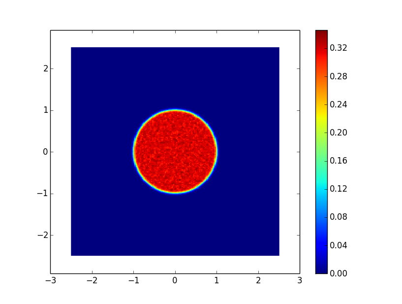
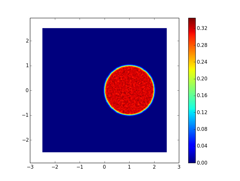
Figure 1. Study of the quadratic confinement for $n=300$ without constraint (left) and with the constraint (55) (right). We see that the constrained measure is a unit disk centered at $(1,0)$.

In this simple case, the Hamiltonian in (50) is only modified by a constant, so we expect the Metropolis rejection rate (Step (5) in Algorithm 4.5) to scale like $\mathrm{O}(\Delta t^{3})$ when $\Delta t\to 0$. In Figure 2, we plot this rate in log-log coordinates (setting here $n=50$ to reduce the computation time). The slope is indeed close to $3$, which confirms our expectation.

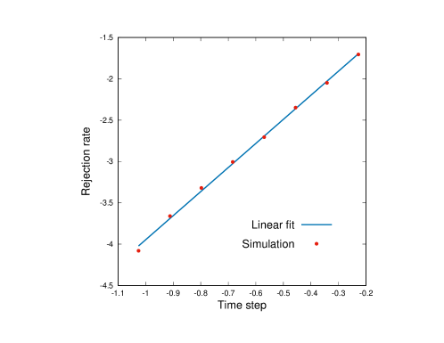
Figure 2. Study of the rejection rate of the Metropolis–Hastings selection rule with $n=50$ (Step (5) in Algorithm 4.5) in log-log coordinates. The slope of the linear fit is about $2.9$.

In order to show that the translation phenomenon is specific to the quadratic confinement, we first consider the case of a quartic confinement potential, namely $V(x)=|x|^{4}/4$ subject to the constraint (55) with $c=0.5$. This choice for $V$ together with $\varphi$ defined in (55) satisfies Assumption 3.6, so that Theorem 3.7 applies. However, no analytic solution is a priori available because the rotational symmetry is lost. The unconstrained equilibrium measure in Figure 3 (left) shows a depletion of the density around $(0,0)$. In Figure 3 (right), we observe that the shape of the distribution is significantly modified by the constraint, and does not possess any rotational invariance. As could have been expected, the particles close to the origin feel a weaker confinement, so the distribution is more concentrated near the outer edge.

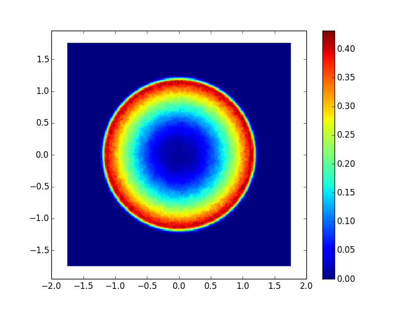
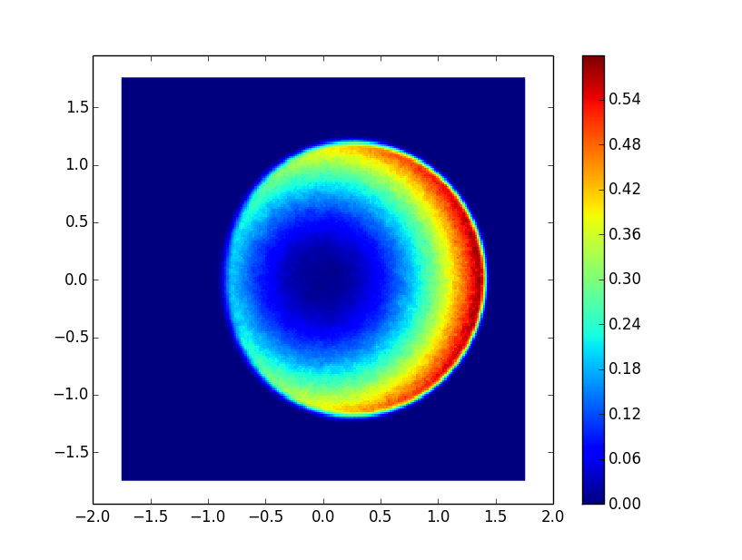
Figure 3. Study of the quartic confinement for $n=300$ without constraint (left) and with the constraint (55) (right). The shape of the equilibrium measure is significantly distorted by the constraint.

Another interesting case is when the confinement is weaker than quadratic, e.g. $V(x)=\frac{2}{3}|x|^{\frac{3}{2}}$, for which Theorem 3.7 still applies. The results are shown in Figure 4, considering again the constraint (55) with $c=0.5$. We observe that the shape of the distribution also significantly changes by spreading in the direction of the constraint. This can be interpreted as follows: since the confinement is stronger at the origin, the more likely way to observe a fluctuation of the barycenter (or less costly in terms of energy) is in this case to spread the distribution.

Quite interestingly, for both potentials the distribution obtained as $c\to+\infty$ seems to reach a limiting ellipsoidal shape, under an appropriate rescaling (figures not shown here). Studying more precisely these limiting shapes and the rate at which they appear is an interesting open problem.

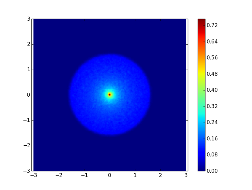
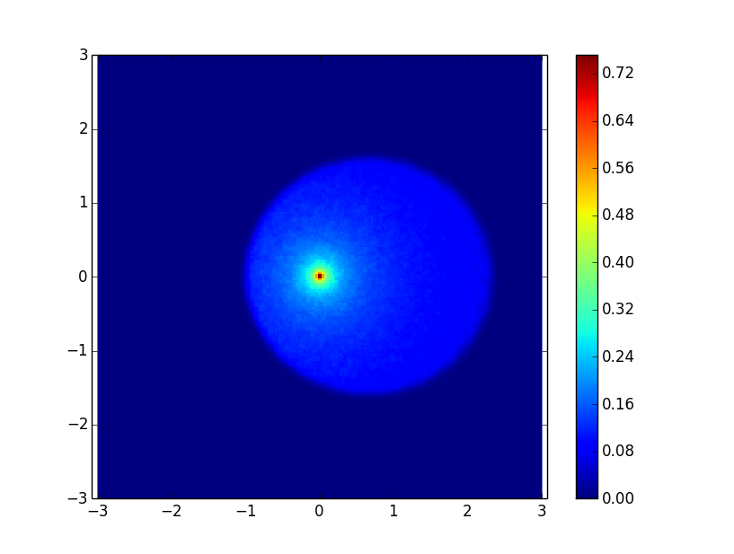
Figure 4. Study of the weak confinement for $n=300$ without constraint (left) and with the constraint (55) (right). The constraint now spreads the equilibrium measure to the right.

4.2.2. Other constraints in dimension two

In order to illustrate the efficiency of our algorithm in situations richer than the linear constraint with a linear function $\varphi$, we now present two other cases. First, we keep a linear constraint with $V(x)=|x|^{2}$, but set

$$\forall\,x\in\mathbb{R}^{2},\quad\varphi(x)=c-\frac{\cos(5x_{1})+\cos(5x_{2})}{2},$$

where $x_{1}$ and $x_{2}$ denote here the first and second coordinates of $x\in\mathbb{R}^{2}$. This choice is motivated by Remark 3.11: since the Laplacian of $\varphi$ takes positive and negative values, we expect the particles to concentrate in some regions of $\mathbb{R}^{2}$, possibly leading to a phase separation. Note also that, in order for the two last conditions in Assumption 3.6 to be satisfied, we need to choose $c\in(-1,1)$. We set again $n=300$ but $\Delta t=0.4$ to reduce the rejection rate. The other parameters are the same as in Section 4.2.1. We plot in Figure 5 the result of the simulation for $c=0.2$ and $c=0.5$. The particles concentrate in the regions where the cosines are higher, which seems to lead to a phase separation when $c$ comes close to $1$.

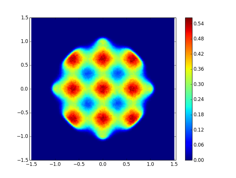
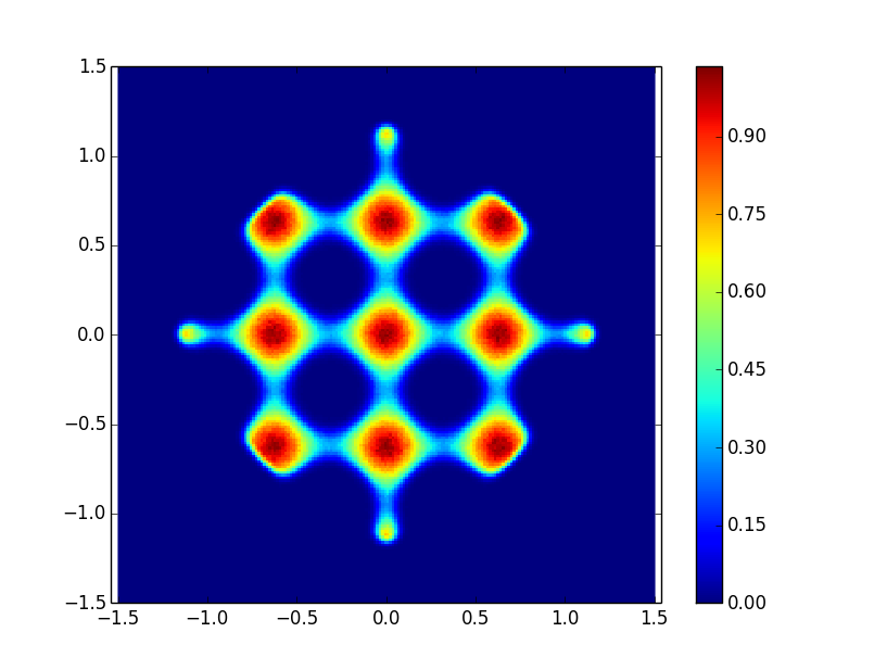
Figure 5. Study of the cosine constraint for $n=300$ with $c=0.2$ (left) and $c=0.5$ (right). A phase separation appears as the particles are constrained to stay around the local maxima of the cosines.

In order to illustrate the results of Section 3.3, we consider a quadratic constraint $\xi:(\mathbb{R}^{d})^{n}\to\mathbb{R}$ of the form

(56) $$\forall\,x\in(\mathbb{R}^{d})^{n},\quad\xi(x)=\frac{1}{n^{2}}\sum_{i,j=1}^{n}\psi(x_{i},x_{j}),$$

with, for $x,y\in\mathbb{R}^{2}$,

(57) $$\psi(x,y)=\phi(x-y),\quad\mbox{and}\quad\phi(x)=c-|x|.$$

A motivation for this choice is to modify the rigidity of the gas by constraining the particles to be closer or farther apart one from another in average. In order to make this rigidity anisotropic, we also consider (57) with

(58) $$\forall\,x\in\mathbb{R}^{2},\quad\phi(x)=c-|x_{1}|.$$

The choice (58) modifies the rigidity only in one direction. For illustration we take $V(x)=|x|^{4}/4$, $n=50$, $\Delta t=0.5$, $T=10^{6}$ (we take a lower number of particles because the constraint makes the dynamics quite stiff). We set $c=1$ for (57) and $c=0.5$ for (58), which forces the particles to move away from each other. These choices for $\psi$ satisfy the conditions of Proposition 3.13, and the application $Q$ defined in (36) can be proved to be convex, so Assumption 3.12 is satisfied and Theorem 3.14 applies. The distribution obtained for the constraint (57), presented in Figure 6 (left), shows that the more likely way for the particles to be repelled by the constraint induced by $\psi$ is to move away from the center and concentrate on the edge, compared to Figure 3 (left). For the constraint (58), we clearly observe in Figure 6 (right) the effect of anisotropy.

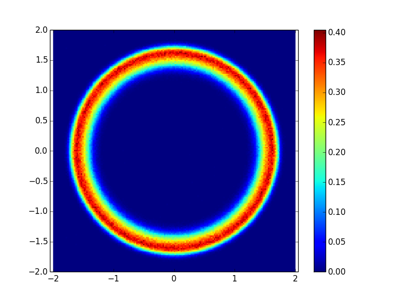
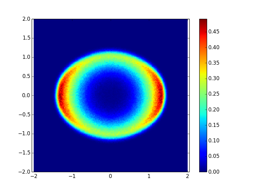
Figure 6. Study of the quartic confinement for $n=50$ with the quadratic statistics constraint (56)-(57) where $c=1$ (left), and with the constraint (58) with $c=0.5$ (right). This has to be compared to the unconstrained distribution in Figure 3 (left).

4.2.3. A one dimensional example

We consider the Gaussian Unitary Ensemble (GUE), which is a degenerate two-dimensional Coulomb gas for which the particles are confined on the real axis. It corresponds in a sense to (8) with $d=1$, $V(x)=|x|^{2}$ but $g(x)=-\log|x|$, and $\beta_{n}=n^{2}$. It is known that the equilibrium measure is then the Wigner semi–circle law, and we refer for instance to [5] for a large deviations study. We can apply Theorem 2.1 for the linear constraint (55). In this case, the Wigner semi–circle law is indeed translated by a factor $c$ (figure not shown here).

Next, in order to illustrate a case which is not covered by our analysis, we want to sample the spectrum of those matrices whose determinant is equal to $\pm 1$. In our context, this corresponds to the configurations $x\in(\mathbb{R}^{d})^{n}$ with $\prod_{i=1}^{n}|x_{i}|=1$. By taking the logarithm, this constraint is actually of the form (45) (by Remark 4.2 the conditioned probability measure (42) does not depend on the parametrization) with

(59) $$\forall\,x\in(\mathbb{R}^{d})^{n},\quad\xi(x)=\frac{1}{n}\sum_{i=1}^{n}\log|x_{i}|-c.$$

We plot in Figure 7 the distribution for $n=300$, $T=10^{5}$ and $\Delta t=0.05$ for the unconstrained log-gas, and for the constraint (59) with $c=-0.5$ and $c=0$ for $\Delta t=0.01$ (starting with particles equally spaced over the interval $[-1,1]$). We observe what looks like a symmetrized Marchenko–Pastur distribution. Actually Remark 3.11 suggests that the effective potential of the constrained distribution is $|\cdot|^{2}-\alpha\log|\cdot|$ for some $\alpha>0$, which is not that far from the Laguerre potential $|\cdot|-\alpha\log|\cdot|$.

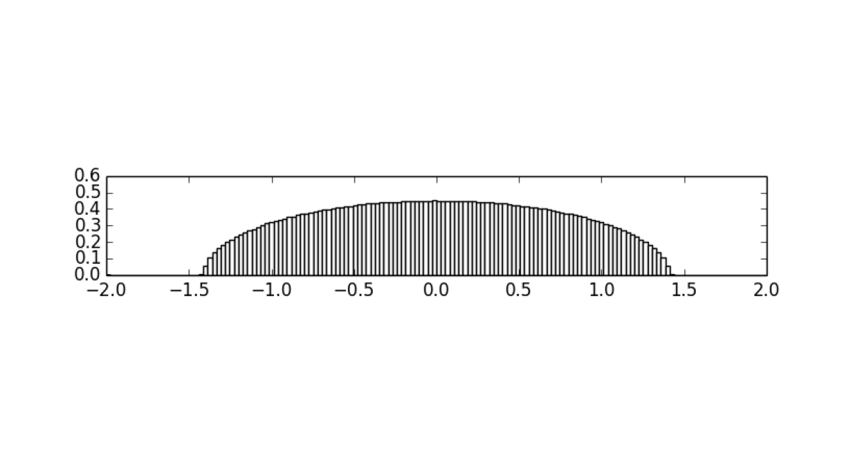
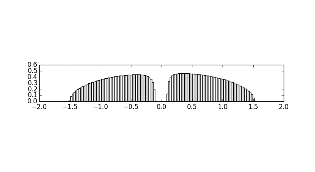
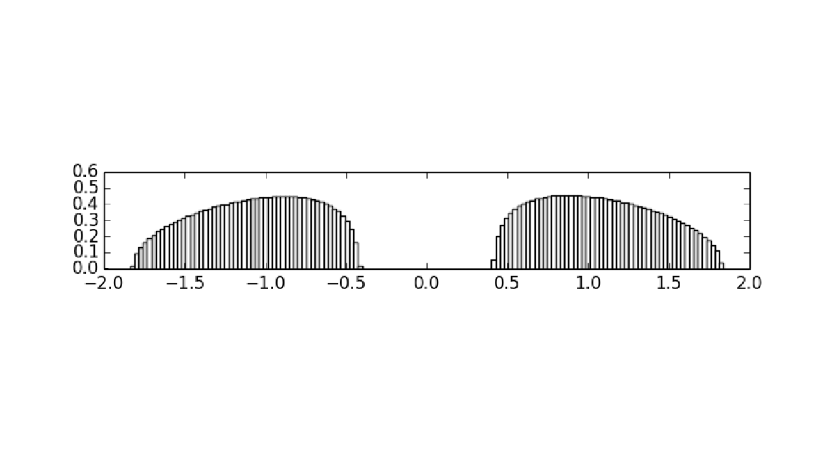
Figure 7. Study of the one dimensional log-gas for $n=300$ without constraint (top) and with the constraint (55) for $c=-0.5$ (middle) and $c=0$ (bottom). This corresponds to a deformation of the semi–circle distribution.

Appendix A Proof of Theorem 2.1

This section is devoted to the proof of Theorem 2.1. First, the following lemma is some sort of quantitative Wasserstein version of [9, Lemma C.1].

Lemma A.1 (Translation).

Let $d\geq 1$, $p\geq 1$, $\mu_{1},\mu_{2}\in\mathcal{P}_{p}(\mathbb{R}^{d})$ and $\varphi:\mathbb{R}^{d}\to\mathbb{R}$ be a measurable function. Then for all $m_{1},m_{2}\in\mathbb{R}^{d}$,

$$\mathrm{d}_{\mathrm{W}_{p}}^{p}(\mu_{1}*\delta_{m_{1}},\mu_{2}*\delta_{m_{2}})\leq 2^{p-1}|m_{1}-m_{2}|^{p}+2^{p-1}\mathrm{d}^{p}_{\mathrm{W}_{p}}(\mu_{1},\mu_{2}).$$

Moreover, if $m_{i}=a\left(\int\varphi\,\mathrm{d}\mu_{i}\right)$ for $i=1,2$ and $a\in\mathbb{R}^{d}$, then

$$\mathrm{d}_{\mathrm{W}_{p}}(\mu_{1}*\delta_{m_{1}},\mu_{2}*\delta_{m_{2}})\leq 2^{\frac{p-1}{p}}(1+|a|^{p}\|\varphi\|^{p}_{\mathrm{Lip}})^{\frac{1}{p}}\mathrm{d}_{\mathrm{W}_{p}}(\mu_{1},\mu_{2}).$$

Note that the right hand side is infinite if $\varphi$ is not Lipschitz.

Proof.

We have, by using the infimum formulation (17) of the distance $\mathrm{d}_{\mathrm{W}_{p}}$,

$$\mathrm{d}_{\mathrm{W}_{p}}^{p}(\mu_{1}*\delta_{m_{1}},\mu_{2}*\delta_{m_{2}})\leq 2^{p-1}|m_{1}-m_{2}|^{p}+2^{p-1}\mathrm{d}_{\mathrm{W}_{p}}^{p}(\mu_{1},\mu_{2}),$$

where we used the convexity inequality $|u+v|^{p}\leq 2^{p-1}(|u|^{p}+|v|^{p})$ valid for all $u,v\in\mathbb{R}^{d}$. Then, since $p\mapsto\mathrm{d}_{\mathrm{W}_{p}}$ is monotonic for $p\geq 1$, it holds

$$|m_{1}-m_{2}|=\left|a\left(\int_{\mathbb{R}^{d}}\varphi\,\mathrm{d}(\mu_{1}-\mu_{2})\right)\right|\leq|a|\|\varphi\|_{\mathrm{Lip}}\mathrm{d}_{\mathrm{W}_{1}}(\mu_{1},\mu_{2})\leq|a|\|\varphi\|_{\mathrm{Lip}}\mathrm{d}_{\mathrm{W}_{p}}(\mu_{1},\mu_{2}),$$

which is the claimed estimate. ∎

The following lemma is a $d$-dimensional version of the factorization lemma in [17]. It expresses a non obvious independence between the center of mass and the shape of the cloud of particles distributed according to $P_{n}$. As noticed in [17], it reminds the structure of certain continuous spins systems such as in [11, 44].

Lemma A.2 (Factorization).

Suppose that the assumptions of Theorem 2.1 are satisfied, and define $u=(v,\ldots,v)\in(\mathbb{R}^{d})^{n}$. Let $\pi$ and $\pi^{\perp}$ be the orthogonal projections in $(\mathbb{R}^{d})^{n}$ on the linear subspaces

$$L=\mathbb{R}u\quad\text{and}\quad L^{\perp}=\left\{x\in(\mathbb{R}^{d})^{n}:x\cdot u=0\right\}.$$

Then, abridging $X_{n}$ into $X$, the following properties hold:

• for all $x\in(\mathbb{R}^{d})^{n}$, denoting $s(x)=\frac{x_{1}+\cdots+x_{n}}{n}\in\mathbb{R}^{d}$, we have

  $$\pi(x) =(s(x)\cdot v)u=\big{(}(s(x)\cdot v)v,\ldots,(s(x)\cdot v)v\big{)},$$

  $$\pi^{\perp}(x) =x-\pi(x)=x-(s(x)\cdot v)u=\big{(}x_{1}-(s(x)\cdot v)v,\ldots,x_{n}-(s(x)\cdot v)v\big{)};$$

• $\pi(X)$ and $\pi^{\perp}(X)$ are independent random vectors;

• $\pi(X)$ is Gaussian with law $\mathcal{N}\left(0,\frac{n}{2\beta_{n}}\right)u$, so that $s(X)\cdot v$ has law $\mathcal{N}\left(0,\frac{n}{2\beta_{n}}\right)$;

• $\pi^{\perp}(X)$ has law of density proportional to $x\in L^{\perp}\mapsto\mathrm{e}^{-\beta_{n}H_{n}(x)}$ with respect to the trace of the Lebesgue measure on the linear subspace $L^{\perp}$ of $\mathbb{R}^{dn-1}$.

Proof of Lemma A.2.

Since $|v|=1$, we have $|u|=\sqrt{n}$, so the orthonormal projection on $L$ reads, for $x\in(\mathbb{R}^{d})^{n}$,

$$\pi(x)=\frac{x\cdot u}{|u|^{2}}u=\left(\frac{1}{n}\sum_{i=1}^{n}x_{i}\cdot v\right)u=\big{(}s(x)\cdot v\big{)}u.$$

The expression of $\pi^{\perp}$ follows easily. For all $x\in(\mathbb{R}^{d})^{n}$, from $x=\pi(x)+\pi^{\perp}(x)$ we get

$$|x|^{2}=|\pi(x)|^{2}+|\pi^{\perp}(x)|^{2}.$$

On the other hand, for all $i,j\in\{1,\ldots,n\}$ it holds

$$x_{i}-x_{j} =\pi(x)_{i}+\pi^{\perp}(x)_{i}-\pi(x)_{j}-\pi^{\perp}(x)_{j}$$

$$=s(x)+\pi^{\perp}(x)_{i}-s(x)-\pi^{\perp}(x)_{j}$$

$$=\pi^{\perp}(x)_{i}-\pi^{\perp}(x)_{j}.$$

Since $V(x)=|x|^{2}$, it follows that, for all $x=(x_{1},\ldots,x_{n})\in(\mathbb{R}^{d})^{n}$,

$$H_{n}(x)=\frac{1}{n}|x|^{2}+\frac{1}{n^{2}}\sum_{i\neq j}g(x_{i}-x_{j})=\frac{1}{n}|\pi(x)|^{2}+H_{n}\big{(}\pi^{\perp}(x)\big{)}.$$

Now, let $u_{1},\ldots,u_{dn}$ be an orthogonal basis of $(\mathbb{R}^{d})^{n}=\mathbb{R}^{dn}$ with $u_{1}=u/\sqrt{n}\in L$. For all $x\in(\mathbb{R}^{d})^{n}$ we write $x=\sum_{i=1}^{dn}t_{i}(x)u_{i}$. We have $\pi(x)=t_{1}(x)u_{1}=(s(x)\cdot v)u$ and $\pi^{\perp}(x)=\sum_{i=2}^{dn}t_{i}(x)u_{i}$. Then we have, for all bounded measurable $f:L\to\mathbb{R}$ and $g:L^{\perp}\to\mathbb{R}$,

$$\mathbb{E}\Big{[}f\big{(}\pi(X)\big{)}g\big{(}\pi^{\perp}(X)\big{)}\Big{]} =Z^{-1}\int_{(\mathbb{R}^{d})^{n}}f\big{(}\pi(x)\big{)}g\big{(}\pi^{\perp}(x)\big{)}\,\mathrm{e}^{-\frac{\beta_{n}}{n}|\pi(x)|^{2}}\,\mathrm{e}^{-\beta_{n}H_{n}(\pi^{\perp}(x))}\mathrm{d}x_{1}\cdots\mathrm{d}x_{n}$$

$$=Z^{-1}\left(\int_{\mathbb{R}}f(t^{\prime})\,\mathrm{e}^{-\frac{\beta_{n}}{n}|t^{\prime}|^{2}}\mathrm{d}t^{\prime}\right)\left(\int_{\mathbb{R}^{dn-1}}g(t^{\prime\prime})\,\mathrm{e}^{-\beta_{n}H_{n}(t^{\prime\prime})}\mathrm{d}t^{\prime\prime}\right),$$

where $t^{\prime}=t_{1}u_{1}$, $\mathrm{d}t^{\prime}=\mathrm{d}t_{1}$, $t^{\prime\prime}=\sum_{i=2}^{dn}t_{i}u_{i}$ and $\mathrm{d}t^{\prime\prime}=\prod_{i=2}^{dn}\mathrm{d}t_{i}$. This concludes the proof of the last two points of the lemma. ∎

We can now turn to the proof of Theorem 2.1.

Proof of Theorem 2.1.

Thanks to Lemma A.2, we have, denoting again by $u=(v,\ldots,v)\in(\mathbb{R}^{d})^{n}$,

$$\mathrm{Law}\left(X_{n}\,\left|\,\frac{1}{n}\sum_{i=1}^{n}\varphi(X_{i})=0\right.\right) =\mathrm{Law}\left(X_{n}\,\left|\,\frac{1}{n}\sum_{i=1}^{n}X_{n,i}\cdot v=c\right.\right)$$

$$=\mathrm{Law}\left(X_{n}\,\Big{|}\,s(X_{n})\cdot v=c\right)$$

$$=\mathrm{Law}\left(X_{n}\,\Big{|}\,\big{(}s(X_{n})\cdot v\big{)}u=cu\right)$$

$$=\mathrm{Law}\left(X_{n}\,\Big{|}\,\pi(X_{n})=cu\right)$$

$$=\mathrm{Law}\left(cu+\pi^{\perp}(X_{n})\right)$$

(60) $$=\mathrm{Law}\big{(}\widetilde{X}_{n}\big{)},$$

where $\widetilde{X}_{n}=cu+\pi^{\perp}(X_{n})=cu+X_{n}-\pi(X_{n})$. We also have

$$\widetilde{X}_{n}=\Big{(}\big{(}c-s(X_{n})\cdot v\big{)}v+X_{n,1},\ldots,\big{(}c-s(X_{n})\cdot v\big{)}v+X_{n,n}\Big{)}\quad\text{where}\quad s(X_{n})=\frac{X_{n,1}+\cdots+X_{n,n}}{n}.$$

In other words (recall that $\varphi(x)=x\cdot v-c$)

$$\widetilde{X}_{n}=\left(X_{n,1}-\frac{1}{n}\sum_{i=1}^{n}\varphi(X_{n,i})v,\ldots,X_{n,n}-\frac{1}{n}\sum_{i=1}^{n}\varphi(X_{n,i})v\right),$$

so that

$$\widetilde{\mu}_{n}=\frac{1}{n}\sum_{i=1}^{n}\delta_{\widetilde{X}_{n,i}}=\mu_{n}*\delta_{m_{n}}\quad\text{where}\quad\mu_{n}=\frac{1}{n}\sum_{i=1}^{n}\delta_{X_{n,i}}\quad\text{and}\quad m_{n}=v\int\varphi\,\mathrm{d}\mu_{n}.$$

Thanks to the assumptions on $V$ and $g$ we know that the equilibrium measure $\mu_{\star}$ is the uniform distribution on a ball of radius $1$. Now we note that $\|\varphi\|_{\mathrm{Lip}}\leq 1$ and $\int\varphi\,\mathrm{d}\mu_{\star}=c$, so that by Lemma A.1 and denoting by $\mu^{\varphi}=\delta_{cv}*\mu_{\star}$, for all $p\geq 1$,

(61) $$\mathrm{d}_{\mathrm{W}_{p}}(\widetilde{\mu}_{n},\mu^{\varphi})\leq 2^{1-1/p}(1+|v|^{p})^{1/p}\mathrm{d}_{\mathrm{W}_{p}}(\mu_{n},\mu_{\star})=2\mathrm{d}_{\mathrm{W}_{p}}(\mu_{n},\mu_{\star}).$$

On the other hand, the large deviations principle – see [14, Proof of Theorem 1.1(4)] and [21] for the fact that the condition (9) ensures that $(\beta_{n})_{n}$ diverges fast enough – gives, for any $\varepsilon>0$,

(62) $$\sum_{n}\mathbb{P}\big{(}\mathrm{d}_{\mathrm{BL}}(\mu_{n},\mu_{\star})\geq\varepsilon\big{)}<\infty.$$

Alternatively we could use the concentration of measure [15, Theorem 1.5] and get the result for $\mathrm{d}_{\mathrm{W}_{1}}$ as well. This summable convergence in probability towards a non-random limit, known as complete convergence [53], is equivalent, via Borel–Cantelli lemmas, to stating that almost surely, $\lim_{n\to\infty}\mathrm{d}_{\mathrm{BL}}(\mu_{n},\mu_{\star})=0$, regardless of the way we defined the random variables $X_{n}$ and thus the random measures $\mu_{n}$ on the same probability space.

In order to upgrade the convergence from $\mathrm{d}_{\mathrm{BL}}$ to $\mathrm{d}_{\mathrm{W}_{p}}$ for all $p\geq 1$ we note that, from [15, Theorem 1.12], there exists $r_{0}>0$ such that, for all $r\geq r_{0}$,

(63) $$\sum_{n}\mathbb{P}\left(\max_{1\leq k\leq n}|X_{n,k}|\geq r\right)<\infty.$$

Now for all $p\geq 1$ and all $\mu,\nu\in\mathcal{P}(\mathbb{R}^{d})$ supported in the ball of $\mathbb{R}^{d}$ of radius $r\geq 1$, we have

$$\mathrm{d}_{\mathrm{W}_{p}}^{p}(\mu,\nu)\leq(2r)^{p-1}\mathrm{d}_{\mathrm{W}_{1}}(\mu,\nu)\leq r(2r)^{p-1}\mathrm{d}_{\mathrm{BL}}(\mu,\nu).$$

Also, by combining (62) and (63), we obtain that for all $p\geq 1$ and all $\varepsilon>0$,

(64) $$\sum_{n}\mathbb{P}\big{(}\mathrm{d}_{\mathrm{W}_{p}}(\mu_{n},\mu_{\star})\geq\varepsilon\big{)}<\infty.$$

By the Borel–Cantelli lemma, for all $p\geq 1$, almost surely, $\lim_{n\to\infty}\mathrm{d}_{\mathrm{W}_{p}}(\mu_{n},\mu_{\star})=0$, regardless of the way we define the random variables $X_{n}$ on the same probability space. Finally, since $p\mapsto\mathrm{d}_{\mathrm{W}_{p}}$ is monotonic in $p$, we can make the almost sure event valid for all $p$ by taking the intersection of all the almost sure events obtained for integer values of $p$.

By combining (64) with (61), we obtain that for all $p\geq 1$ and $\varepsilon>0$,

(65) $$\sum_{n}\mathbb{P}\big{(}\mathrm{d}_{\mathrm{W}_{p}}(\widetilde{\mu}_{n},\mu^{\varphi})\geq\varepsilon\big{)}<\infty.$$

Now if $Y_{n}$ is a random vector of $(\mathbb{R}^{d})^{n}$ such that $\mathrm{Law}(Y_{n})=\mathrm{Law}(X_{n}\mid\varphi(X_{n,1})+\cdots+\varphi(X_{n,n})=0)$ then, denoting by $\mu_{n}^{Y}=\frac{1}{n}\sum_{i=1}^{n}\delta_{Y_{n,i}}$, using (60) and the fact that $\mu^{\varphi}$ is deterministic, we get

$$\mathrm{d}_{\mathrm{W}_{p}}(\mu_{n}^{Y},\mu^{\varphi})\overset{\mathrm{d}}{=}\mathrm{d}_{\mathrm{W}_{p}}(\widetilde{\mu}_{n},\mu^{\varphi}).$$

Therefore, from (65) we get, for all $p\geq 1$ and all $\varepsilon>0$,

$$\sum_{n}\mathbb{P}\big{(}\mathrm{d}_{\mathrm{W}_{p}}(\mu_{n}^{Y},\mu^{\varphi})\geq\varepsilon\big{)}<\infty.$$

By the Borel–Cantelli lemma, for all $p\geq 1$, almost surely, $\lim_{n\to\infty}\mathrm{d}_{\mathrm{W}_{p}}(\mu_{n}^{Y},\mu^{\varphi})=0$, regardless of the way we define the random variables $Y_{n}$ on the same probability space. Finally, since $\mathrm{d}_{\mathrm{W}_{p}}$ is monotonic in $p$, we can make the almost sure event valid for all $p$ by taking the intersection of all the almost sure events obtained for integer values of $p$. ∎

Note that the above proof relies crucially, via Lemma A.2, on the quadratic nature of $V$. However the Coulomb nature of $g$ is less crucial and the result should remain essentially valid provided that the convergence to the equilibrium measure holds, for instance at the level of generality of the assumptions of the large deviations principle in [14].

Appendix B Proofs of Section 3.1

We start with the proof of the abstract Gibbs conditioning principle.

Proof of Theorem 3.1.

Since $I$ is a good rate function, it is lower semicontinuous with compact level sets. The set $\mathscr{I}_{B}$ defined in (24) is not empty because the infimum is finite by (23), $B$ is closed and $I$ has compact level sets, so the infimum is attained at least for one measure. Moreover, $\mathscr{I}_{B}$ is closed by lower semicontinuity of $I$. Now, since

$$\frac{1}{\beta_{n}}\log\mathbb{P}\left(Z_{n}\in A_{\varepsilon}\ \Big{|}\ Z_{n}\in B\right)=\frac{1}{\beta_{n}}\log\mathbb{P}\left(Z_{n}\in A_{\varepsilon}\cap B\right)-\frac{1}{\beta_{n}}\log\mathbb{P}\left(Z_{n}\in B\right),$$

the result follows from an upper bound on $\mathbb{P}(A_{\varepsilon}\cap B)$ and a lower bound on $\mathbb{P}(B)$. The upper bound of the large deviations principle implies that

(66) $$\limsup_{n\to+\infty}\frac{1}{\beta_{n}}\log\mathbb{P}\left(Z_{n}\in A_{\varepsilon}\cap B\right)\leq-\inf_{\overline{A_{\varepsilon}\cap B}}I.$$

Assume first that $\overline{A_{\varepsilon}\cap B}\neq\emptyset$. Since $A_{\varepsilon}=\{z\in\mathcal{Z},\ \mathrm{d}(z,\mathscr{I}_{B})>\varepsilon\}$, the lower semi-continuity of $I$ shows that (see [14, Section 2.5]) there exists $c_{\varepsilon}>0$ for which

$$\inf_{\overline{A_{\varepsilon}\cap B}}I\geq c_{\varepsilon}+\inf_{B}I,$$

so that

(67) $$\limsup_{n\to+\infty}\frac{1}{\beta_{n}}\log\mathbb{P}\left(Z_{n}\in A_{\varepsilon}\cap B\right)\leq-\inf_{B}I-c_{\varepsilon}.$$

If $\overline{A_{\varepsilon}\cap B}=\emptyset$, the infimum in the right hand side of (66) is equal to $+\infty$ so that (67) still holds. The lower bound for the set $B$ reads

$$\liminf_{n\to+\infty}\frac{1}{\beta_{n}}\log\mathbb{P}\left(Z_{n}\in B\right)\geq-\inf_{\mathring{B}}I.$$

Since $B$ satisfies (23), it holds

$$\limsup_{n\to+\infty}-\frac{1}{\beta_{n}}\log\mathbb{P}\left(Z_{n}\in B\right)\leq\inf_{B}I,$$

which, together with (67), leads to (25).

Finally, if $Z_{n}^{\prime}\sim\mathrm{Law}(Z_{n}\mid Z_{n}\in B)$ and if we define the $Z_{n}^{\prime}$’s on the same probability space then, for all $\varepsilon>0$, thanks to (9), by the Borel–Cantelli lemma, $\sum_{n}\mathbb{P}(Z_{n}^{\prime}\in A_{\varepsilon})<\infty$ and thus, almost surely, $Z_{n}^{\prime}\not\in A_{\varepsilon}$ for large enough $n$. Since the set $A_{\varepsilon}$ depends on $\varepsilon>0$, by taking $\varepsilon\to 0$ with $\varepsilon\in\mathbb{Q}$, we obtain that almost surely, $\lim_{n\to\infty}\mathrm{d}(Z_{n}^{\prime},\mathscr{I}_{B})=0$. ∎

We next recall elements of proof for the properties of the rate function $\mathcal{E}$.

Proof of Proposition 3.3.

Consider a probability measure $\mu\in D_{\mathcal{E}}$, so

$$\int_{\mathbb{R}^{d}}V(x)\mu(\mathrm{d}x)+\iint_{\mathbb{R}^{d}\times\mathbb{R}^{d}}g(x-y)\mu(\mathrm{d}x)\mu(\mathrm{d}y)<+\infty.$$

Since $V$ satisfies Assumption 3.2 and therefore beats $g$ at infinity (in particular when $d=2$), we have

$$\int_{\mathbb{R}^{d}}|x|^{p}\mu(\mathrm{d}x)<+\infty,$$

for $1<p<q$. Thus $D_{\mathcal{E}}\subset\mathcal{P}_{p}(\mathbb{R}^{d})$.

The strict convexity of $\mathcal{E}$ is due to a Bochner-type positivity of the interaction kernel. See for instance [48, Chapter I, Lemma 1.8], [46], or [14, Section 3] for $d=2$ and [33, Theorems 1.15 and 1.16] or [14, Lemma 3.1] for $d\geq 3$. The uniqueness of the minimizer follows from the strict convexity. The compactness of its support relies on the behaviour of $V$ at infinity, see for instance [48, Chapter I, Theorem 1.3] for $d=2$ and [14, Theorem 1.2] for $d\geq 3$. Finally, since the minimizer of $\mathcal{E}$ over $\mathcal{P}(\mathbb{R}^{d})$ has compact support, the three problems in (26) clearly coincide. ∎

We finally present the proof of Corollary 3.5, which is a consequence of Theorem 3.1 and the Borel–Cantelli lemma.

Proof of Corollary 3.5.

Under $P_{n}$, the empirical measure $\mu_{n}$ associated to $X_{n}$ satisfies a LDP in the $p$-Wasserstein topology with good rate function $\mathcal{E}$. Since $B$ is assumed to be a closed continuity set for the $p$-Wasserstein topology, the set $\mathscr{E}_{B}$ defined in (29) is closed and non-empty by Theorem 3.1.

For simplicity we denote by

$$\mu_{n}^{Y}=\frac{1}{n}\sum_{i=1}^{n}\delta_{Y_{n,i}}$$

the empirical measure associated to $Y_{n}$, where $Y_{n}\sim\mathrm{Law}(X_{n}\,|\,\mu_{n}\in B)$. For any $\varepsilon>0$, we define the set $A_{\varepsilon}$ as in Theorem 3.1. Then, there exists $c_{\varepsilon}>0$ such that

$$\sum_{n}\mathbb{P}\big{(}\mathrm{d}_{\mathrm{W}_{p}}(\mu_{n}^{Y},\mathscr{E}_{B})>\varepsilon\big{)} =\sum_{n}\mathbb{P}\big{(}\mathrm{d}_{\mathrm{W}_{p}}(\mu_{n},\mathscr{E}_{B})>\varepsilon\ \big{|}\ \mu_{n}\in B\big{)}$$

$$=\sum_{n}\mathbb{P}\big{(}\mu_{n}\in A_{\varepsilon}\ \big{|}\ \mu_{n}\in B\big{)}$$

$$\leq C\sum_{n}\mathrm{e}^{-\beta_{n}c_{\varepsilon}}<+\infty,$$

for some $C>0$. Since $\beta_{n}\gg n$ thanks to (9), the Borell–Cantelli lemma implies that

$$\lim_{n\to\infty}\mathrm{d}_{\mathrm{W}_{p}}\big{(}\mu_{n}^{Y},\mathscr{E}_{B}\big{)}=0,$$

almost surely in any probability space, which concludes the proof. ∎

Appendix C Proof of Theorem 3.7

The proof is decomposed into four steps. We first show that under Assumption 3.6, the set $B$ is an $I$-continuity set for the electrostatic energy $\mathcal{E}$. We next show that any minimizer of $\mathcal{E}$ over $B$ has a compact support, and hence the minimizer is actually unique. The last two steps characterize the minimizer through (32).

Step 1: $I$-continuity

Let us first show that $B\subset\mathcal{P}_{p}(\mathbb{R}^{d})$ is closed for the $p$-Wasserstein topology by showing that $B^{c}=\{\mu\in\mathcal{P}_{p}(\mathbb{R}^{d})\,|\,\mu(\varphi)>0\}$ is open. Take $\mu\in B^{c}$ and $\nu$ such that $\mathrm{d}_{\mathrm{W}_{p}}(\mu,\nu)\leq\varepsilon^{\frac{1}{p}}$ for some $\varepsilon>0$. By definition of the $p$-Wasserstein distance it holds

(68) $$\sup_{\begin{subarray}{c}f\in\mathrm{L}^{1}(\mu),\,g\in\mathrm{L}^{1}(\nu)\\ f(x)\leq g(y)+|x-y|^{p}\end{subarray}}\left(\int_{\mathbb{R}^{d}}f\,\mathrm{d}\mu-\int_{\mathbb{R}^{d}}g\,\mathrm{d}\nu\right)\leq\varepsilon.$$

Since $\|\varphi\|_{\infty,p}<+\infty$, for any $\mu,\nu\in\mathcal{P}_{p}(\mathbb{R}^{d})$ it holds $\varphi\in L^{1}(\nu)\cap L^{1}(\mu)$. Moreover, $\|\varphi\|_{\mathrm{Lip}}<+\infty$ and $\varphi$ cannot be a constant function because this would contradict the existence of $\mu_{\pm}$ in Assumption 3.6, so $\|\varphi\|_{\mathrm{Lip}}>0$. As a result, for $|x-y|\geq 1$ we have

$$|\varphi(x)-\varphi(y)|\leq\|\varphi\|_{\mathrm{Lip}}|x-y|\leq\|\varphi\|_{\mathrm{Lip}}|x-y|^{p}.$$

Therefore, $\varphi/\|\varphi\|_{\mathrm{Lip}}$ satisfies the inf-convolution condition in (68) and we may pick $f=g=\varphi/\|\varphi\|_{\mathrm{Lip}}$ so that

$$\int_{\mathbb{R}^{d}}\frac{\varphi}{\|\varphi\|_{\mathrm{Lip}}}\,\mathrm{d}\mu-\int_{\mathbb{R}^{d}}\frac{\varphi}{\|\varphi\|_{\mathrm{Lip}}}\,\mathrm{d}\nu\leq\varepsilon,$$

which becomes

$$\nu(\varphi)\geq\mu(\varphi)-\varepsilon\|\varphi\|_{\mathrm{Lip}}>0\quad\mathrm{for}\quad\varepsilon<\frac{\mu(\varphi)}{\|\varphi\|_{\mathrm{Lip}}}.$$

As a result, $B^{c}$ is open and $B$ is closed for the $p$-Wasserstein topology.

We now prove that $B$ is an $I$-continuity set, namely that (31) holds. By the same reasoning as above, the existence of $\mu_{-}\in D_{\mathcal{E}}$ such that $\mu_{-}(\varphi)<0$ ensures that $\mu_{-}\in\mathring{B}$ (recall that $\mu_{-}\in\mathcal{P}_{p}(\mathbb{R}^{d})$ by Proposition 3.3) so

$$\inf_{\mathring{B}}\mathcal{E}<+\infty.$$

Since $B$ is closed and $\mathcal{E}$ has compact level sets, there exists $\bar{\mu}$ such that

$$\mathcal{E}(\bar{\mu})=\inf_{B}\mathcal{E}.$$

If $\bar{\mu}(\varphi)<0$, it holds $\bar{\mu}\in\mathring{B}$ and the proof is complete. Thus we may assume that $\bar{\mu}(\varphi)=0$ and, by considering a minimizing sequence, for any $\varepsilon>0$ we may find $\mu_{\varepsilon}\in\mathring{B}$ such that

(69) $$\mathcal{E}(\mu_{\varepsilon})\leq\inf_{\mathring{B}}\mathcal{E}+\varepsilon.$$

For $t\in[0,1]$, we introduce $\mu_{t}=t\mu_{\varepsilon}+(1-t)\bar{\mu}\in D_{\mathcal{E}}$. Since $\bar{\mu}(\varphi)=0$ it holds $\mu_{t}\in\mathring{B}$ for any $t\in(0,1]$. By convexity of $\mathcal{E}$ on its domain we have

$$\mathcal{E}(\mu_{t})\leq t\mathcal{E}(\mu_{\varepsilon})+(1-t)\mathcal{E}(\bar{\mu}).$$

We now proceed by contradiction by assuming that $\mathcal{E}(\bar{\mu})=\inf_{\mathring{B}}\mathcal{E}-\eta$ for some $\eta>0$. Recalling (69) we have, for some $\varepsilon>0$ and any $t\in(0,1]$,

$$\mathcal{E}(\mu_{t})\leq t\left(\inf_{\mathring{B}}\mathcal{E}+\varepsilon\right)+(1-t)\left(\inf_{\mathring{B}}\mathcal{E}-\eta\right)=\inf_{\mathring{B}}\mathcal{E}+t\varepsilon-(1-t)\eta.$$

Considering

$$t<\frac{\eta}{\varepsilon+\eta},$$

we obtain that $\mu_{t}\in\mathring{B}$ with

$$\mathcal{E}(\mu_{t})<\inf_{\mathring{B}}\mathcal{E},$$

which is a contradiction. Therefore, (31) holds true.

Step 2: the minimizer is unique and has compact support

We now show that any minimizer $\mu^{\varphi}$ has a compact support, before turning to uniqueness. We detail the proof for $d\geq 3$ following [14] by highlighting the necessary modifications, and leave the proof for $d=2$ to the reader (which is deduced from [48, Chapter I, Theorem 1.3]). We introduce

$$\zeta=\inf_{B}\mathcal{E}$$

and, for any compact $K$,

$$\zeta_{K}=\inf_{B_{K}}\mathcal{E},\quad\text{where}\quad B_{K}=\{\mu\in B\ |\ \mathrm{supp}(\mu)\subset K\}.$$

By Assumption 3.6, $B_{K}$ is non empty for $K$ large enough (consider $\mu_{-}(\,\cdot\,\mathds{1}_{K})/\mu_{-}(K)$ for $K$ large enough). By Assumption 3.2, for any constant $C$ the set

(70) $$K=\left\{x\in\mathbb{R}^{d},\ V(x)\leq C\right\}$$

is compact. In all what follows, we assume that $V\geq 0$. Since $V$ is lower bounded and defined up to a constant, there is no loss of generality in this assumption.

Let us show that $\zeta=\zeta_{K}$ for $C$ large enough when $K$ is defined by (70). Since the infimums on $B$ and $\mathring{B}$ coincide, we can consider a measure $\mu\in B$ such that $\mu(\varphi)<0$ and $\mathcal{E}(\mu)\leq\zeta+1$. If $\mu(K)=1$, the measure has compact support and we are done, so we assume that $\mu(K)<1$. The goal of the following computations is to build a measure $\mu_{K}\in B$ supported in $K$ such that $\mathcal{E}(\mu_{K})<\mathcal{E}(\mu)$; this contradiction will show that $\zeta$ and $\zeta_{K}$ are equal. Let us first show that $\mu(K)>0$ for $C$ large enough. Indeed,

$$\zeta+1\geq\mathcal{E}(\mu)=\underbrace{\int_{K}V\,\mathrm{d}\mu}_{\geq 0}+\int_{K^{c}}V\,\mathrm{d}\mu+\underbrace{J(\mu)}_{\geq 0}\geq C(1-\mu(K)),$$

which shows that $\mu(K)>0$ if $C>\zeta+1$. We may therefore define the restriction

$$\mu_{K}(\,\cdot\,)=\frac{\mu(K\cap\cdot\,)}{\mu(K)}.$$

Since $\mu(K)<1$, we define similarly $\mu_{K^{c}}$. The measure $\mu$ then reads

$$\mu=\mu(K)\mu_{K}+(1-\mu(K))\mu_{K^{c}}.$$

Moreover, we chose $\mu$ such that $\mu(\varphi)<0$, so it holds $\mu_{K}\in B_{K}$ for $C$ large enough. Using the positivity of $V$ and $J$ (since $d\geq 3$ and so $g\geq 0$) and $\mu(K)<1$, we obtain that

$$\mathcal{E}(\mu)= \ \mu(K)\int_{\mathbb{R}^{d}}V\,\mathrm{d}\mu_{K}+(1-\mu(K))\underbrace{\int_{\mathbb{R}^{d}}V\,\mathrm{d}\mu_{K^{c}}}_{\geq C}+\mu(K)^{2}J(\mu_{K})$$

$$+2\mu(K)(1-\mu(K))\underbrace{J(\mu_{K},\mu_{K^{c}})}_{\geq 0}+(1-\mu(K))^{2}\underbrace{J(\mu_{K^{c}})}_{\geq 0}$$

$$\geq \ \mu(K)^{2}J(\mu_{K})+\mu(K)^{2}\int_{\mathbb{R}^{d}}V\,\mathrm{d}\mu_{K}+(1-\mu(K))C$$

$$\geq \ \mu(K)^{2}\mathcal{E}(\mu_{K})+(1-\mu(K))C.$$

Let us proceed by contradiction by assuming that $\mathcal{E}(\mu_{K})\geq\mathcal{E}(\mu)$, which leads to

$$\mathcal{E}(\mu)\geq\mu(K)^{2}\mathcal{E}(\mu)+(1-\mu(K))C.$$

Since $\mathcal{E}(\mu)\leq\zeta+1$ we obtain

$$(\zeta+1)(1-\mu(K)^{2})\geq(1-\mu(K))C.$$

Simplifying by $1-\mu(K)$ we have

$$2(\zeta+1)\geq C,$$

which is absurd for $C>2(\zeta+1)$. Since $\mu_{K}\in B$ for $C$ large enough, this shows that $\zeta$ and $\zeta_{K}$ coincide and that any minimizer has compact support.

In the above proof, the only modification with respect to previous works (see for instance [14]) is to check that the restricted measure $\mu_{K}$ satisfies the constraint for $C$ large enough. This is done by picking the measure $\mu$ close to the minimum and such that $\mu(\varphi)<0$. The same strategy can be used in the situation where $d=2$ by writing

$$\mathcal{E}(\mu)=\iint_{\mathbb{R}^{d}\times\mathbb{R}^{d}}\left(\frac{V(x)+V(y)}{2}-\log|x-y|\right)\mu(\mathrm{d}x)\mu(\mathrm{d}y),$$

and adapting [48, Chapter I, Theorem 1.3] since $V(x)+V(y)$ dominates $\log|x-y|$ at infinity by Assumption 3.2.

The minimizer is unique due to the strict convexity of $\mathcal{E}$, see Proposition 3.3, and the linearity of the constraint.

Step 3: Lagrange multiplier

We now turn to a first step towards the expression of $\mu^{\varphi}$ involving a Lagrange multiplier $\alpha$. We adapt the proof of [4, Theorem 3.1] by introducing the following subset of $\mathbb{R}^{2}$:

(71) $$R=\big{\{}\big{(}\mathcal{E}(\mu)-\mathcal{E}(\mu^{\varphi})+a_{0},\mu(\varphi)+a_{1}\big{)}:a_{0}>0,\,a_{1}>0,\,\mu\in D_{\mathcal{E}}\big{\}}.$$

Since $\mathcal{E}$ is convex on its domain $D_{\mathcal{E}}$ (which is convex), $R$ is a non empty convex subset of $\mathbb{R}^{2}$ that does not contain $(0,0)$ (recall also that $D_{\mathcal{E}}\subset\mathcal{P}_{p}(\mathbb{R}^{d})$ so the constraint takes finite values). Separating $R$ from $(0,0)$ with a hyperplane (see [4, Corollary 1.41]), this ensures the existence of $(\alpha_{0},\alpha_{1})\in\mathbb{R}^{2}\setminus\{(0,0)\}$ such that, for any $\mu\in D_{\mathcal{E}}$ and $a_{0},a_{1}>0$ it holds

$$\alpha_{0}\big{(}\mathcal{E}(\mu)-\mathcal{E}(\mu^{\varphi})+a_{0}\big{)}+\alpha_{1}\big{(}\mu(\varphi)+a_{1}\big{)}>0.$$

By taking $a_{1}\to-\mu^{\varphi}(\varphi)\geq 0$ and $\mu=\mu^{\varphi}$ in the above equation, we obtain that $\alpha_{0}\geq 0$. Then, choosing $\mu=\mu^{\varphi}$, $a_{0}\to 0$ and $a_{1}>-\mu^{\varphi}(\varphi)\geq 0$ we find $\alpha_{1}\geq 0$. Taking $a_{0},a_{1}\to 0$, we obtain

(72) $$\forall\,\mu\in D_{\mathcal{E}},\quad\alpha_{0}\mathcal{E}(\mu^{\varphi})\leq\alpha_{0}\mathcal{E}(\mu)+\alpha_{1}\mu(\varphi).$$

We now prove that $\alpha_{0}>0$ by contradiction. If $\alpha_{0}=0$, (72) becomes

$$\forall\,\mu\in D_{\mathcal{E}},\quad 0\leq\alpha_{1}\mu(\varphi).$$

Since $\alpha_{1}\neq 0$ in this case, the above equation contradicts Assumption 3.6 by taking $\mu=\mu_{-}$, so $\alpha_{0}>0$ and we may renormalize (72) into

(73) $$\forall\,\mu\in D_{\mathcal{E}},\quad\mathcal{E}(\mu^{\varphi})\leq\mathcal{E}(\mu)+\alpha\mu(\varphi),$$

where we set $\alpha=\alpha_{1}/\alpha_{0}\geq 0$.

Finally, we show that either $\mu^{\varphi}=\mu_{\star}$, in which case $\alpha=0$, or $\mu^{\varphi}(\varphi)=0$ and $\alpha>0$. First, if $\mu_{\star}\in B$, $\mu_{\star}$ satisfies the constraint and we know from Proposition 3.3 that it solves (32) with $\alpha=0$. Otherwise, it holds $\mu_{\star}(\varphi)>0$. Since $\mathcal{E}(\mu_{\star})<\mathcal{E}(\mu^{\varphi})$ because $\mu_{\star}$ is the unique global minimizer of $\mathcal{E}$, we then obtain from (73) with the choice $\mu=\mu_{\star}$ that $\alpha>0$. Choosing next $\mu=\mu^{\varphi}$ in (73) shows that $\mu^{\varphi}(\varphi)=0$, so the minimizer actually saturates the constraint.

Step 4: potential equation

In order to derive the equation for $\mu^{\varphi}$, we follow [14, Section 4] by introducing the modified potential and electrostatic energy, for $\mu\in\mathcal{P}(\mathbb{R}^{d})$,

$$V_{\alpha}=V+\alpha\varphi,\quad\mathcal{E}_{\alpha}(\mu)=\int_{\mathbb{R}^{d}}V_{\alpha}(x)\mu(\mathrm{d}x)+J(\mu).$$

Since the case when $\alpha=0$ corresponds to no-conditioning and we already know that the equation is satisfied by the equilibrium measure in this case, we restrict our attention to the situation in which $\alpha>0$ and $\mu^{\varphi}(\varphi)=0$. We define next, for any $\mu\in D_{\mathcal{E}}$,

$$\forall\,t\in(0,1),\quad\psi(t)=\mathcal{E}_{\alpha}\big{(}(1-t)\mu^{\varphi}+t\mu\big{)}.$$

Because of (73) and the convexity of $\psi$, it holds $\psi^{\prime}(0)\geq 0$, so that

$$0 \leq\psi^{\prime}(0)=\int_{\mathbb{R}^{d}}V_{\alpha}\,\mathrm{d}(\mu-\mu^{\varphi})+2J(\mu^{\varphi},\mu-\mu^{\varphi})$$

$$\leq\int_{\mathbb{R}^{d}}V_{\alpha}\,\mathrm{d}\mu+2J(\mu^{\varphi},\mu)-\left(\int_{\mathbb{R}^{d}}V_{\alpha}\,\mathrm{d}\mu^{\varphi}+2J(\mu^{\varphi})\right)$$

$$\leq\int_{\mathbb{R}^{d}}(V_{\alpha}+2U_{\mu^{\varphi}})\,\mathrm{d}\mu-C_{\varphi},$$

where we set $U_{\mu^{\varphi}}=\mu^{\varphi}*g$ and

$$C_{\varphi}=\int_{\mathbb{R}^{d}}V_{\alpha}\,\mathrm{d}\mu^{\varphi}+2J(\mu^{\varphi})=\int_{\mathbb{R}^{d}}(V+2U_{\mu^{\varphi}})\,\mathrm{d}\mu^{\varphi},$$

since $\mu^{\varphi}(\varphi)=0$. The above inequality may be rewritten as

$$\forall\,\mu\in D_{\mathcal{E}},\quad\int_{\mathbb{R}^{d}}(V_{\alpha}+2U_{\mu^{\varphi}}-C_{\varphi})\,\mathrm{d}\mu\geq 0,$$

which proves the second line of (32). Recall indeed that, by definition, a property holds quasi-everywhere if and only if it holds almost surely for all probability measures with finite energy. Moreover, the measures $\mu$ and $\mu^{\varphi}$ belonging to $D_{\mathcal{E}}\subset\mathcal{P}_{p}(\mathbb{R}^{d})$, they satisfy condition (4) so that the quantity $J(\mu,\mu^{\varphi})$ is well-defined following the remark below (20).

Let us now prove the first line in (32) by contradiction. Assume that there is $x\in\mathrm{supp}(\mu^{\varphi})$ such that $V_{\alpha}(x)+2U_{\mu^{\varphi}}(x)>C_{\varphi}$. Since $\mu^{\varphi}$ has compact support, $U_{\mu^{\varphi}}$ is lower semi-continuous [33, page 59]. Since $V$ is lower semi-continuous and $\varphi$ is Lipschitz hence continuous, $V_{\alpha}+2U_{\mu^{\varphi}}$ is lower semi-continuous. There exists therefore a neighborhood $\mathcal{U}$ of $x$ and $\varepsilon>0$ such that

$$\forall\,x\in\mathcal{U},\quad V_{\alpha}(x)+2U_{\mu^{\varphi}}(x)\geq C_{\varphi}+\varepsilon.$$

Integrating with respect to $\mu^{\varphi}$ and using $\mu^{\varphi}(\varphi)=0$ leads to

$$C_{\varphi}=\int_{\mathbb{R}^{d}}(V_{\alpha}+2U_{\mu^{\varphi}})\,\mathrm{d}\mu^{\varphi} =\int_{\mathcal{U}}(V+2U_{\mu^{\varphi}})\,\mathrm{d}\mu^{\varphi}+\int_{\mathbb{R}^{d}\setminus\mathcal{U}}(V+2U_{\mu^{\varphi}})\,\mathrm{d}\mu^{\varphi}$$

$$\geq(C_{\varphi}+\varepsilon)\mu^{\varphi}(\mathcal{U})+\int_{\mathbb{R}^{d}\setminus\mathcal{U}}(V+2U_{\mu^{\varphi}})\,\mathrm{d}\mu^{\varphi}.$$

Since $V_{\alpha}+2U_{\mu^{\varphi}}\geq C_{\varphi}$ quasi-everywhere and $\mu^{\varphi}\in D_{\mathcal{E}}$, the above inequality becomes

$$C_{\varphi}=\int_{\mathbb{R}^{d}}(V_{\alpha}+2U_{\mu^{\varphi}})\,\mathrm{d}\mu^{\varphi}\geq C_{\varphi}+\varepsilon\mu^{\varphi}(\mathcal{U}).$$

We reach a contradiction by noting that $\mu^{\varphi}(\mathcal{U})>0$ since $\mathcal{U}$ is a neighborhood of $x\in\mathrm{supp}(\mu^{\varphi})$ (using the definition of the support), which proves the first line of (32).

Appendix D Proof of Theorem 3.14

We outline the proof of Theorem 3.14, which follows the same lines as in the linear case.

Proof.

We show below that the set $B\subset\mathcal{P}_{p}(\mathbb{R}^{d})$ defined in (35) is closed for the $p$-Wasserstein topology under Assumption 3.12. For this, we show that $B^{c}$ is open by picking $\mu\in\mathcal{P}_{p}(\mathbb{R}^{d})$ such that $Q(\mu)>0$ and using again that, for $\varepsilon>0$ and $\nu\in\mathcal{P}_{p}(\mathbb{R}^{d})$ such that $\mathrm{d}_{\mathrm{W}_{p}}(\mu,\nu)\leq\varepsilon^{\frac{1}{p}}$, it holds, by (18),

(74) $$\sup_{\begin{subarray}{c}f\in\mathrm{L}^{1}(\mu),\,g\in\mathrm{L}^{1}(\nu)\\ f(x)\leq g(y)+|x-y|^{p}\end{subarray}}\left(\int_{\mathbb{R}^{d}}f\,\mathrm{d}\mu-\int_{\mathbb{R}^{d}}g\,\mathrm{d}\nu\right)\leq\varepsilon.$$

First, by Assumption 3.12, we note that for any $\mu,\nu\in\mathcal{P}_{p}(\mathbb{R}^{d})$ it holds $\|U_{\mu}^{\psi}\|_{\infty,p}<+\infty$ and $\|U_{\nu}^{\psi}\|_{\infty,p}<+\infty$. Therefore, $U_{\mu}^{\psi}\in L^{1}(\mu)\cap L^{1}(\nu)$ and $U_{\nu}^{\psi}\in L^{1}(\mu)\cap L^{1}(\nu)$ for any probability measures $\mu,\nu$ with moments of order $p$. Next, by (37), it holds $\|U_{\mu}^{\psi}\|_{\mathrm{Lip}}\leq C_{\mathrm{Lip}}$ and $\|U_{\nu}^{\psi}\|_{\mathrm{Lip}}\leq C_{\mathrm{Lip}}$. We assume for now that these norms are non-zero, so we may first choose $f=g=U_{\mu}^{\psi}/\|U_{\mu}^{\psi}\|_{\mathrm{Lip}}$, which leads to

(75) $$Q(\mu)-\iint_{\mathbb{R}^{d}\times\mathbb{R}^{d}}\psi(x,y)\nu(\mathrm{d}x)\mu(\mathrm{d}y)\leq\varepsilon\|U_{\mu}^{\psi}\|_{\mathrm{Lip}}.$$

Symmetrically we take $f=g=-U_{\nu}^{\psi}/\|U_{\nu}^{\psi}\|_{\mathrm{Lip}}$, which leads to

(76) $$\iint_{\mathbb{R}^{d}\times\mathbb{R}^{d}}\psi(y,x)\nu(\mathrm{d}x)\mu(\mathrm{d}y)-Q(\nu)\leq\varepsilon\|U_{\nu}^{\psi}\|_{\mathrm{Lip}}.$$

By summing (75) and (76) and using the symmetry of $\psi$, we obtain

(77) $$Q(\nu)\geq Q(\mu)-\varepsilon\big{(}\|U_{\nu}^{\psi}\|_{\mathrm{Lip}}+\|U_{\mu}^{\psi}\|_{\mathrm{Lip}}\big{)}\geq Q(\mu)-2C_{\mathrm{Lip}}\varepsilon.$$

This shows that $Q(\nu)>0$ for $\varepsilon<Q(\mu)/(2C_{\mathrm{Lip}})$. To finish the argument, we consider the cases where the Lipschitz norm of the potentials generated by $\mu$ and $\nu$ may be zero. Suppose first that $\|U_{\mu}^{\psi}\|_{\mathrm{Lip}}=0$. This implies the existence of $c_{\mu}\in\mathbb{R}$ such that

(78) $$\forall\,x\in\mathbb{R}^{d},\quad\int_{\mathbb{R}^{d}}\psi(x,y)\mu(\mathrm{d}y)=c_{\mu}.$$

Integrating the above equation with respect to $\mu$ shows that $c_{\mu}=Q(\mu)>0$. As a result, if $\|U_{\mu}^{\psi}\|_{\mathrm{Lip}}=0$ and $\nu$ is such that $\|U_{\nu}^{\psi}\|_{\mathrm{Lip}}>0$ we can consider (76), which becomes (integrating (78) with respect to $\nu$)

$$Q(\nu)\geq Q(\mu)-\varepsilon\|U_{\nu}^{\psi}\|_{\mathrm{Lip}}\geq Q(\mu)-\varepsilon C_{\mathrm{Lip}}.$$

In this case, $Q(\nu)>0$ for $\varepsilon<Q(\mu)/C_{\mathrm{Lip}}$. Then, if $\|U_{\nu}^{\psi}\|_{\mathrm{Lip}}=0$ it holds, for some $c_{\nu}\in\mathbb{R}$,

(79) $$\forall\,x\in\mathbb{R}^{d},\quad\int_{\mathbb{R}^{d}}\psi(x,y)\nu(\mathrm{d}y)=c_{\nu}.$$

Integrating with respect to $\mu$ and using the symmetry of $\psi$ we obtain that $c_{\nu}=c_{\mu}>0$. Integrating next (79) with respect to $\nu$ shows that $Q(\nu)=c_{\mu}=Q(\mu)>0$. Finally, if $\|U_{\mu}^{\psi}\|_{\mathrm{Lip}}>0$ but $\|U_{\nu}^{\psi}\|_{\mathrm{Lip}}=0$, (79) holds with $c_{\nu}=Q(\nu)$ so that (75) becomes

$$Q(\nu)\geq Q(\mu)-\varepsilon C_{\mathrm{Lip}},$$

and the same conclusion follows. As a result, in any case the measures $\nu$ such that $\mathrm{d}_{\mathrm{W}_{p}}(\mu,\nu)\leq\varepsilon^{\frac{1}{p}}$ for $\varepsilon<Q(\mu)/(2C_{\mathrm{Lip}})$ belong to $B^{c}$ so that $B^{c}$ is open and $B$ is closed in the $p$-Wasserstein topology.

We next show that $B$ is an $I$-continuity set. The existence of $\mu_{-}\in D_{\mathcal{E}}\subset\mathcal{P}_{p}(\mathbb{R}^{d})$ such that $Q(\mu_{-})<0$ ensures that

$$\inf_{\mathring{B}}\mathcal{E}<+\infty.$$

Since $\mathcal{E}$ has compact level sets and $B$ is closed, there exists $\bar{\mu}$ such that

$$\mathcal{E}(\bar{\mu})=\inf_{B}\mathcal{E}.$$

If $Q(\bar{\mu})<0$, $I$-continuity is proven, so we may assume that $Q(\bar{\mu})=0$. Like in the linear case, we may take $\mu_{\varepsilon}\in\mathring{B}$ such that

$$\mathcal{E}(\mu_{\varepsilon})\leq\inf_{\mathring{B}}\mathcal{E}+\varepsilon,$$

and consider the convex combination $\mu_{t}=t\mu_{\varepsilon}+(1-t)\bar{\mu}$ for $t\in(0,1)$. The convexity of $Q$ shows that, for any $t\in(0,1)$ it holds

$$Q(\mu_{t})\leq tQ(\mu_{\varepsilon})+(1-t)Q(\bar{\mu})<0,$$

so that $\mu_{t}\in\mathring{B}$. Proceeding by contradiction by supposing that $\mathcal{E}(\bar{\mu})<\inf_{\mathring{B}}\mathcal{E}$, we obtain that for $t>0$ small enough it holds $\mu_{t}\in\mathring{B}$ and

$$\mathcal{E}(\mu_{t})<\inf_{\mathring{B}}\mathcal{E},$$

which is a contradiction, proving that $B$ is an $I$-continuity set.

One can next follow Step 2 of the proof of Theorem 3.7 to show that the minimizer $\mu^{\psi}$ is unique with compact support.

At this stage, the remaining statements in Theorem 3.14 can be proved as for Theorem 3.7. In particular, we can introduce a set similar to (71) by setting

$$R=\big{\{}\big{(}\mathcal{E}(\mu)-\mathcal{E}(\mu^{\varphi})+a_{0},Q(\mu)+a_{1}\big{)}:a_{0}>0,\,a_{1}>0,\,\mu\in D_{\mathcal{E}}\big{\}}.$$

The set $R$ is convex by convexity of $Q$, so the same convex separation theorem can be used, and we can show that there exists $\alpha\geq 0$ such that

$$\forall\,\mu\in D_{\mathcal{E}},\quad\mathcal{E}(\mu^{\psi})\leq\mathcal{E}(\mu)+\alpha Q(\mu).$$

In this procedure, we use the existence of $\mu_{\pm}$ from Assumption 3.12 in order to reproduce the qualification of constraint argument. This leads to computations where the interaction energy $J$ is replaced by

$$J_{\alpha}(\mu,\nu)=J(\mu,\nu)+\alpha\iint_{\mathbb{R}^{d}\times\mathbb{R}^{d}}\psi(x,y)\mu(\mathrm{d}x)\mu(\mathrm{d}y),$$

from which (39) follows by mimicking Step 4 of the proof of Theorem 3.7. ∎

As a final comment, let us insist on the importance of the convexity of $Q$ for the above proof to be valid.

References

- [1] G. Akemann & M. Cikovic – “Products of random matrices from fixed trace and induced Ginibre ensembles”, J. Phys. A 51 (2018), no. 18, p. 184002, 34.
- [2] L. Ambrosio, N. Fusco & D. Pallara – Functions of Bounded Variation and Free Discontinuity Problems, Oxford Mathematical Monographs, vol. 254, Clarendon Press Oxford, 2000.
- [3] S. N. Armstrong, S. Serfaty & O. Zeitouni – “Remarks on a constrained optimization problem for the Ginibre ensemble”, Potential Anal. 41 (2014), no. 3, p. 945–958.
- [4] V. Barbu & T. Precupanu – Convexity and Optimization in Banach Spaces, Mathematics and its Applications, vol. 10, Springer Science & Business Media, 2012.
- [5] G. Ben Arous & A. Guionnet – “Large deviations for Wigner’s law and Voiculescu’s non-commutative entropy”, Probab. Theory Relat. Fields 108 (1997), no. 4, p. 517–542.
- [6] C. Berg, J. P. R. Christensen & P. Ressel – Harmonic Analysis on Semigroups: Theory of Positive Definite and Related Functions, Graduate Texts in Mathematics, vol. 100, Springer, 1984.
- [7] Berman, Robert J. – “On large deviations for Gibbs measures, mean energy and Gamma-convergence”, Constructive Approximation 48 (2018), no. 1, p. 3–30.
- [8] R. J. Berman – “The Coulomb gas, potential theory and phase transitions”, preprint arXiv:1811.10249 (2018).
- [9] C. Bordenave, P. Caputo & D. Chafaï – “Circular law theorem for random Markov matrices”, Probab. Theory Relat. Fields 152 (2012), no. 3-4, p. 751–779.
- [10] J.-P. Bouchaud & M. Potters – Financial applications of random matrix theory: a short review, The Oxford Handbook of Random Matrix Theory, 824–850, Oxford Univ. Press, Oxford, 2011.
- [11] D. Chafaï – “Glauber versus Kawasaki for spectral gap and logarithmic Sobolev inequalities of some unbounded conservative spin systems”, Markov Process. Relat. 9 (2003), no. 3, p. 341–362.
- [12] D. Chafaï & G. Ferré – “Simulating Coulomb and log-gases with Hybrid Monte Carlo algorithms”, J. Statist. Phys. 174 (2018), no. 3, p. 692–714.
- [13] D. Chafaï, G. Ferré & G. Stoltz – “Coulomb gases under constraint: some theoretical and numerical results”, preprint arXiv:1907.05803v1 (2019).
- [14] D. Chafaï, N. Gozlan & P.-A. Zitt – “First-order global asymptotics for confined particles with singular pair repulsion”, Ann. Appl. Probab. 24 (2014), no. 6, p. 2371–2413.
- [15] D. Chafaï, A. Hardy & M. Maïda – “Concentration for Coulomb gases and Coulomb transport inequalities”, J. Funct. Anal. 275 (2018), no. 6, p. 1447–1483.
- [16] D. Chafaï & S. Péché – “A note on the second order universality at the edge of Coulomb gases on the plane”, J. Stat. Phys. 156 (2014), no. 2, p. 368–383.
- [17] D. Chafaï & J. Lehec – “On Poincaré and logarithmic Sobolev inequalities for a class of singular Gibbs measures”, To appear in Geometric Aspects of Functional Analysis – Israel Seminar (GAFA) 2017–2019, Lecture Notes in Mathematics 2256
- [18] I. Csiszár – “Sanov property, generalized I-projection and a conditional limit theorem”, Ann. Probab. 12 (1984), no. 3, p. 768–793.
- [19] E. Darve – “Thermodynamic integration using constrained and unconstrained dynamics”, in Free Energy Calculations (C. Chipot & A. Pohorille, eds.), Springer Series in Chemical Physics, vol. 86, Springer, 2007, p. 119–170.
- [20] A. Dembo & O. Zeitouni – Large Deviations Techniques and Applications, Stochastic Modelling and Applied Probability, vol. 38, Springer-Verlag, Berlin, 2010, Corrected reprint of the second (1998) edition.
- [21] P. Dupuis, V. Laschos & K. Ramanan – “Large deviations for configurations generated by Gibbs distributions with energy functionals consisting of singular interaction and weakly confining potentials”, Electron. J. Probab. 25 (2020), paper no. 46.
- [22] L. Erdős & H.-T. Yau – A Dynamical Approach to Random Matrix Theory, Courant Lecture Notes in Mathematics, vol. 28, American Mathematical Society, Providence, RI, 2017.
- [23] L. Evans & R. Gariepy – Measure Theory and Fine Properties of Functions, Studies in Advanced Mathematics, vol. 5, CRC Press, 2018.
- [24] P. J. Forrester – Log-gases and Random Matrices, London Mathematical Society Monographs Series, vol. 34, Princeton University Press, Princeton, NJ, 2010.
- [25] D. García-Zelada – “A large deviation principle for empirical measures on Polish spaces: Application to singular Gibbs measures on manifolds”, Ann. Inst. Henri Poincaré Probab. Stat. 55 (2019), no. 3, p. 1377–1401.
- [26] S. Ghosh & A. Nishry – “Gaussian complex zeros on the hole event: the emergence of a forbidden region”, Comm. Pure Appl. Math. 72 (2019), no. 1, 3–62.
- [27] by same author, “Point processes, hole events, and large deviations: random complex zeros and Coulomb gases”, Constr. Approx. 48 (2018), no. 1, p. 101–136.
- [28] E. Hairer, C. Lubich & G. Wanner – Geometric Numerical Integration: Structure-Preserving Algorithms for Ordinary Differential Equations, Springer Series in Computational Mathematics, vol. 31, Springer Science & Business Media, 2006.
- [29] A. Hardy – “A note on large deviations for 2D Coulomb gas with weakly confining potential”, Electron. Commun. Probab. 17 (2012), paper no. 19.
- [30] A. Koldobsky – Fourier Analysis in Convex Geometry, Mathematical Surveys and Monographs, no. 116, American Mathematical Soc., 2005.
- [31] B. R. La Cour & W. C. Schieve – “A general conditional large deviation principle”, J. Stat. Phys. 161 (2015), no. 1, p. 123–130.
- [32] G. Lambert – “Poisson statistics for Gibbs measures at high temperature”, preprint arXiv:1912.10261v1 (2019).
- [33] N. S. Landkof – Foundations of Modern Potential Theory, Springer-Verlag, 1972, Translated from the Russian by A. P. Doohovskoy, Die Grundlehren der mathematischen Wissenschaften, Band 180.
- [34] G. Le Caër & R. Delannay – “The fixed-trace -Hermite ensemble of random matrices and the low temperature distribution of the determinant of an -Hermite matrix”, J. Phys. A 40 (2007), no. 7, p. 1561–1584.
- [35] T. Leblé & S. Serfaty – “Large deviation principle for empirical fields of Log and Riesz gases”, Invent. Math. 210 (2017), no. 3, p. 645–757.
- [36] T. Lelièvre, M. Rousset & G. Stoltz – Free Energy Computations. A Mathematical Perspective, Imperial College Press, London, 2010.
- [37] by same author, “Langevin dynamics with constraints and computation of free energy differences”, Math. Comp. 81 (2012), no. 280, p. 2071–2125.
- [38] T. Lelièvre, M. Rousset & G. Stoltz – “Hybrid Monte Carlo methods for sampling probability measures on submanifolds”, Numer. Math. 143 (2019), no 2, p. 379–421.
- [39] C. Léonard – “Entropic projections and dominating points”, ESAIM: Probab. Stat. 14 (2010), p. 343–381.
- [40] C. Léonard & J. Najim – “An extension of Sanov’s theorem: application to the Gibbs conditioning principle”, Bernoulli 8 (2002), no. 6, p. 721–743.
- [41] Y. Lu & J. C. Mattingly – “Geometric ergodicity of Langevin dynamics with Coulomb interactions”, Nonlinearity 33 (2020), no. 2, 675–699.
- [42] S. N. Majumdar, C. Nadal, A. Scardicchio & P. Vivo – “Index distribution of Gaussian random matrices”, Phys. Rev. Lett. 103 (2009), p. 220603.
- [43] by same author, “How many eigenvalues of a Gaussian random matrix are positive?”, Phys. Rev. E 83 (2011), p. 041105.
- [44] F. Malrieu – “Logarithmic Sobolev inequalities for some nonlinear PDE’s”, Stoch. Proc. Appl. 95 (2001), no. 1, p. 109–132.
- [45] J.-M. Marin, P. Pudlo, C. P. Robert & R. J. Ryder – “Approximate Bayesian computational methods”, Stat. Comput. 22 (2012), no. 6, p. 1167–1180.
- [46] D. Petz, & F. Hiai Logarithmic energy as an entropy functional. Advances in Differential Equations and Mathematical Physics (Atlanta, GA, 1997), 205–221, Contemp. Math., 217, Amer. Math. Soc., Providence, RI, 1998.
- [47] F. Rassoul-Agha & T. Seppäläinen – A Course on Large Deviations with an Introduction to Gibbs measures, Graduate Studies in Mathematics, vol. 162, American Mathematical Society, Providence, RI, 2015.
- [48] E. B. Saff & V. Totik – Logarithmic Potentials with External Fields, Grundlehren der Mathematischen Wissenschaften, vol. 316, Springer-Verlag, Berlin, 1997.
- [49] S. Serfaty – Coulomb gases and Ginzburg-Landau vortices, Zurich Lectures in Advanced Mathematics, Euro. Math. Soc. (EMS), Zürich, 2015.
- [50] by same author, “Systems of points with Coulomb interactions”, Proceedings of the International Congress of Mathematicians—Rio de Janeiro 2018. Vol. I. Plenary lectures, 935–977, World Sci. Publ., 2018.
- [51] S. Tavaré, D. J. Balding, R. C. Griffiths & P. Donnelly – “Inferring coalescence times from DNA sequence data”, Genetics 145 (1997), no. 2, p. 505–518.
- [52] C. Villani – Topics in Optimal Transportation, Graduate Studies in Mathematics, vol. 58, American Mathematical Society, 2003.
- [53] J. E. Yukich – Probability Theory of Classical Euclidean Optimization Problems, Lecture Notes in Mathematics, vol. 1675, Springer-Verlag, Berlin, 1998.
- [54] E. Zappa, M. Holmes-Cerfon & J. Goodman – “Monte Carlo on manifolds: sampling densities and integrating functions”, Comm. Pure Appl. Math. 71 (2018), no. 12, p. 2609–2647.
- [55] W. Zhang – “Ergodic SDEs on submanifolds and related numerical sampling schemes”, ESAIM Math. Model. Numer. Anal. 54 (2020), no. 2, 391–430.