Exploration by Optimisation in Partial Monitoring

Abstract

We provide a simple, intuitive and efficient algorithm for adversarial $k$-action $d$-outcome partial monitoring games. Let $m\leq d$ denote the maximum number of different observations per action. We show that for non-degenerate locally observable games the $n$-round minimax regret is bounded by $2mk^{3/2}\sqrt{3n\log(k)}$, matching the best known information-theoretic upper bound in this case. The same algorithm also achieves near-optimal regret for full information, bandit and globally observable games. High probability bounds and simple experiments are also provided.

1 Introduction

Partial monitoring is a generalisation of the bandit framework that decouples the loss and the observations. The framework is sufficiently rich to model bandits, linear bandits, full information games, dynamic pricing, bandits with graph feedback and many problems between and beyond these examples. For positive integer $m$ let $[m]=\{1,\dots,m\}$. A finite adversarial partial monitoring game is determined by a signal matrix $\Phi\in\Sigma^{k\times d}$ and loss matrix $\mathcal{L}\in[0,1]^{k\times d}$ where $\Sigma$ is an arbitrary finite set. Both $\Phi$ and $\mathcal{L}$ are known to the learner. The game proceeds over $n$ rounds. First the adversary chooses a sequence $(x_{t})_{t=1}^{n}$ with $x_{t}\in[d]$. In each round $t\in[n]$ the learner chooses an action $A_{t}\in[k]$, suffers loss $\mathcal{L}_{A_{t}x_{t}}$, but only observes the signal $\sigma_{t}=\Phi_{A_{t}x_{t}}$. The regret is

$$\mathfrak{R}_{n}=\max_{a\in[k]}\sum_{t=1}^{n}\left(\mathcal{L}_{A_{t}x_{t}}-\mathcal{L}_{ax_{t}}\right)\,.$$

The minimax regret is

$$\mathfrak{R}_{n}^{*}=\inf_{\pi}\sup_{(x_{t})_{t=1}^{n}}\mathbb{E}\left[\mathfrak{R}_{n}\right]\,,$$

where the expectation is with respect to the randomness in the actions and $\pi$ is the policy of the learner mapping action/observation sequences to distributions over the actions. Our main contribution is a simple and efficient algorithm for finite non-degenerate locally observable partial monitoring games for which

$$\mathfrak{R}_{n}^{*}\leq 2k^{3/2}m\sqrt{3n\log(k)}\,.$$ (1)

The same algorithm is adaptive to other types of game, achieving near-optimal regret for globally observable games, a regret of $\sqrt{2nk\log(k)}$ for bandits and $\sqrt{2n\log(k)}$ for full information games.

Trivial	$\mathfrak{R}_{n}^{*}=0$
Easy	$\mathfrak{R}_{n}^{*}=\Theta(n^{1/2})$
Hard	$\mathfrak{R}_{n}^{*}=\Theta(n^{2/3})$
Hopeless	$\mathfrak{R}_{n}^{*}=\Omega(n)$

Table 1: Classification of finite partial monitoring

Related work

Partial monitoring goes back to the work by Rustichini, [1999], who derived Hannan consistent policies. There has been significant effort in understanding the dependence of the regret on the horizon. The key result is the classification theorem, showing that all finite partial monitoring games lie in one of four categories as illustrated in Table 1. The classification theorem also gives a procedure to decide into which category a given game belongs. Since the game is known in advance, there is no need to learn the classification of the game. This result has been pieced together over about a decade by a number of authors [Cesa-Bianchi et al.,, 2006; Foster and Rakhlin,, 2012; Antos et al.,, 2013; Bartók et al.,, 2014; Lattimore and Szepesvári, 2019a, ]. Ironically, the ‘easy’ games present the greatest challenge for algorithm design and analysis.

The best known bound for an efficient algorithm for ‘easy’ games is $\mathbb{E}[\mathfrak{R}_{n}]\leq C(\Phi,\mathcal{L})\sqrt{n\log(n)}$, where the constant $C(\Phi,\mathcal{L})$ can be arbitrarily large, even for fixed $k$ and $d$ [Foster and Rakhlin,, 2012; Lattimore and Szepesvári, 2019a, ]. Furthermore, the algorithms achieving this bound are complicated to analyse and the proofs yield little insight into the structure of partial monitoring. Recently we proved that for the ‘non-degenerate’ (defined later) subset of easy games, the minimax regret is at most $\mathfrak{R}_{n}^{*}\leq mk^{3/2}\sqrt{2n\log(k)}$ [Lattimore and Szepesvári, 2019b, ]. Unfortunately, however, our proof non-constructively appealed to minimax duality and the Bayesian regret analysis techniques by Russo and Van Roy, [2016]. No algorithm was provided, a deficiency we now resolve.

Partial monitoring has been studied in a variety of contexts. For example, bandits with graph feedback [Alon et al.,, 2015] and a linear feedback setting [Lin et al.,, 2014]. Some authors also consider a variant of the regret that refines the notion of optimality in hopeless games [Rustichini,, 1999; Mannor and Shimkin,, 2003; Perchet,, 2011; Mannor et al.,, 2014]. Our focus is on the adversarial setting, but the stochastic setup is also interesting and is better understood [Bartók et al.,, 2011; Vanchinathan et al.,, 2014; Komiyama et al.,, 2015].

Approach

Our algorithms are based on exponential weights with importance-weighted loss difference estimators [Freund and Schapire,, 1997]. Crucially, the algorithms do not sample from the distribution proposed by exponential weights. Instead, they solve a convex optimisation problem to find a loss difference estimator and new distribution over actions for which the loss cannot be much larger than the proposal distribution and the ‘stability’ term in the bound of exponential weights is minimised. We then prove that the value of the optimisation problem appears in the resulting regret guarantee and provide upper bounds for different classes of games. The most challenging aspect is to prove the existence of a suitable exploration distribution for locally observable non-degenerate games, which follows by combining a minimax theorem with insights from the Bayesian setting. The idea to modify the distribution proposed by exponential weights is reminiscent of the work by McMahan and Streeter, [2009] for bandits with expert advice, though the situation here is rather different.

2 Notation and concepts

We write $\bm{0}$ and $\bm{1}$ for the column vectors of all zeros and all ones respectively. For a positive semidefinite matrix $A$ and vector $x$, we let $\left\|x\right\|_{A}^{2}=x^{\top}Ax$ and $\operatorname{diag}(x)$ be the diagonal matrix with $x$ on the diagonal. We use $\left\|A\right\|_{\infty}=\max_{ij}|A_{ij}|$ for the (entrywise) maximum norm of $A$, which we also use for the special case that $A$ is a vector. The minimum entry of a matrix is $\min(A)=\min_{ij}A_{ij}$. The standard basis vectors are $e_{1},\ldots,e_{d}$; we use the same symbols regardless of the dimension, which should be clear from the context in all cases.

In-trees

An in-tree with vertex set $[k]$ is a set $\mathcal{T}\subseteq[k]\times[k]$ representing the edges of a directed tree with vertices $[k]$. Furthermore, we assume there is a root vertex denoted by $\operatorname{root}_{\mathcal{T}}\in[k]$ such that for all $a\in[k]$ there is a directed path $\operatorname{path}_{\mathcal{T}}(a)\subseteq\mathcal{T}$ from $a$ to the root. The path from the root is the empty set: $\operatorname{path}_{\mathcal{T}}(\operatorname{root}_{\mathcal{T}})=\emptyset$. The figure depicts an in-tree over $k=10$ vertices. The blue (barred) path is $\operatorname{path}_{\mathcal{T}}(a)$.

Partial monitoring

Throughout we fix a partial monitoring game $\mathcal{G}=(\Phi,\mathcal{L})$ with loss matrix $\mathcal{L}\in[0,1]^{k\times d}$ and signal matrix $\Phi\in\Sigma^{k\times d}$. Let $\mathcal{D}=\{\nu\in[0,1]^{d}:\left\|\nu\right\|_{1}=1\}$ and $\mathcal{P}=\{p\in[0,1]^{k}:\left\|p\right\|_{1}=1\}$ be the probability simplices of dimension $d-1$ and $k-1$ respectively. It is helpful to notice that if $p\in\mathcal{P}$ and $\nu\in\mathcal{D}$, then $p^{\top}\mathcal{L}\nu$ is the expected loss suffered by a learner sampling an action from $p$ while the adversary samples its output from $\nu$. Given an action $a\in[k]$ let $C_{a}=\{\nu\in\mathcal{D}:e_{a}^{\top}\mathcal{L}\nu\leq\min_{b\in[k]}e_{b}^{\top}\mathcal{L}\nu\}$ be the set of probability vectors in $\mathcal{D}$ where action $a$ is optimal to play in expectation if the adversary plays randomly according to $\nu$. We call $C_{a}$ the cell of action $a$. Cells are convex polytopes because they are bounded and are determined by finitely many non-strict linear constraints. The collection $\{C_{a}:a\in[k]\}$, illustrated in Fig. 1, is called the cell decomposition.

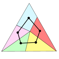
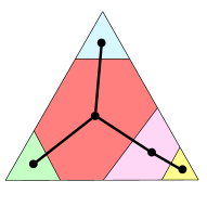
Figure 1: Cell decompositions and neighbourhood graphs for two games with $d=3$ and $k=5$.

Remark 1.

A generalisation of the framework allows $(x_{t})_{t=1}^{n}$ to be chosen in an arbitrary outcome space $\mathcal{X}$ and $\mathcal{L}:[k]\times\mathcal{X}\to[0,1]$ and $\Phi:[k]\times\mathcal{X}\to\Sigma$ are arbitrary functions. Our mathematical results continue to hold in this case with $d=|\mathcal{X}|$, but the proposed algorithms may not be computationally efficient when $|\mathcal{X}|=\infty$. A short discussion of infinite games appears in Section 7.

Neighbourhood graph

A key concept in partial monitoring is the neighbourhood relation, which gives those pairs of potentially optimal actions that can be optimal simultaneously. An action $a$ is called Pareto optimal if $\dim(C_{a})=d-1$ where the dimension of a polytope is defined as the dimension of its affine hull as an affine subspace. The set of Pareto optimal actions is denoted by $\Pi=\{a:\dim(C_{a})=d-1\}$. An action $a$ with $C_{a}\neq\emptyset$ and $\dim(C_{a})\leq d-2$ is called degenerate while actions with $C_{a}=\emptyset$ are dominated. Distinct actions $a$ and $b$ are duplicates if $(e_{a}-e_{b})^{\top}\mathcal{L}=\bm{0}$. Pareto optimal actions $a$ and $b$ are neighbours if $\dim(C_{a}\cap C_{b})=d-2$. More informally, actions are neighbours if their cells share a boundary of dimension $d-2$. Note that $\dim(C_{a}\cap C_{b})=d-1$ is only possible when $a$ and $b$ are duplicates. The neighbourhood relation defines a graph over $[k]$. We let $\mathcal{E}=\{(a,b):a\text{ and }b\text{ are neighbours}\}$ be the set of edges in this graph. A game is called non-degenerate if it has no degenerate actions. Of course, $\dim(\mathcal{D})=d-1$, so actions $a$ with $\dim(C_{a})<d-1$ are optimal on a ‘negligible’ subset of $\mathcal{D}$, where they cannot be uniquely optimal. For the remainder we make the following simplifying assumption.

Assumption 2.

$\mathcal{G}$ is globally observable, non-degenerate and contains no duplicate actions.

There is no particular reason to discard degenerate games except their analysis requires careful handling of certain edge cases, as we discuss briefly in the discussion and extensively in other work [Lattimore and Szepesvári, 2019a, ]. No modifications to the algorithm are required.

Observability

The classification of a partial monitoring game depends on both the loss and signal matrices. What is important to make a non-degenerate game ‘easy’ is that the learner should have some way to estimate the loss differences between neighbouring actions by playing only those actions, a property known as local observability. A game is globally observable if for all edges $e=(a,b)\in\mathcal{E}$ in the neighbourhood graph there exists a function $w_{e}:[k]\times\Sigma\to\mathbb{R}$ such that

$$\mathcal{L}_{ax}-\mathcal{L}_{bx}=\sum_{c=1}^{k}w_{e}(c,\Phi_{cx})\text{ for all }x\in[d]\,.$$ (2)

A non-degenerate game is locally observable if Eq. 2 holds and additionally $w_{e}$ can be chosen so that $w_{e}(c,\sigma)=0$ for all $c\notin\{a,b\}$ and all $\sigma$. Of course, all locally observable games are globally observable.

Remark 3.

The reader should be aware that for arbitrary (possibly degenerate) games the definition of local observability is that there exist estimation vectors such that Eq. 2 holds and $w_{e}(c,\sigma)=0$ unless $e_{c}^{\top}\mathcal{L}=\alpha e_{a}^{\top}\mathcal{L}+(1-\alpha)e_{b}^{\top}\mathcal{L}$ for some $\alpha\in[0,1]$. For non-degenerate games the definitions are equivalent by [Bartók et al.,, 2014, Lemma 11].

The classification theorem we mentioned in the introduction says that

$$\mathfrak{R}_{n}^{*}=\begin{cases}0\,,&\text{if there exists an $a$ with $C_{a}=\mathcal{D}$}\,;\\ \Theta(n^{1/2})\,,&\text{if the game is locally observable}\,;\\ \Theta(n^{2/3})\,,&\text{if the game is globally observable}\,;\\ \Omega(n)\,,&\text{otherwise}\,,\end{cases}$$

where the Big-Oh notation hides game-dependent constants.

Estimation

The following lemma and discussion afterwards shows that for globally observable games Eq. 2 can be chained along paths in the neighbourhood graph to estimate the loss differences between any pair of actions, not just neighbours. Let $\mathcal{H}$ be the set of all functions $G:[k]\times\Sigma\to\mathbb{R}^{k}$.

Lemma 4.

If $\mathcal{G}$ is globally observable, then there exists a function $G\in\mathcal{H}$ such that for all $b,c\in\Pi$,

$$\sum_{a=1}^{k}\left(G(a,\Phi_{ax})_{b}-G(a,\Phi_{ax})_{c}\right)=\mathcal{L}_{bx}-\mathcal{L}_{cx}\,.$$

Proof.

Let $\mathcal{T}\subseteq\mathcal{E}$ be any in-tree over $\Pi$ and for $b\in\Pi$ let $G(a,\sigma)_{b}=\sum_{e\in\operatorname{path}_{\mathcal{T}}(b)}w_{e}(a,\sigma)$. Then

$$\sum_{a=1}^{k}G(a,\Phi_{ax})_{b}=\sum_{a=1}^{k}\sum_{e\in\operatorname{path}_{\mathcal{T}}(b)}w_{e}(a,\Phi_{ax})=\mathcal{L}_{bx}-\mathcal{L}_{\operatorname{root}_{\mathcal{T}}x}\,.$$

The result follows by repeating the argument for $c\in\Pi$ and taking the difference. ∎

Given a distribution $p\in\mathcal{P}\cap(0,1)^{k}$ and $G$ satisfying the conclusion of Lemma 4, it follows that if $A$ is sampled from $p$ and $x\in[d]$ is arbitrary, then for actions $a,b$,

$$\mathbb{E}\left[\frac{(e_{a}-e_{b})^{\top}G(A,\Phi_{Ax})}{p_{A}}\right]=\sum_{c=1}^{k}(e_{a}-e_{b})^{\top}G(c,\Phi_{cx})=\mathcal{L}_{ax}-\mathcal{L}_{bx}\,.$$ (3)

In other words, the function $G$ can be used with importance-weighting to estimate the loss differences. The set of functions that satisfy the consequences of Lemma 4 are denoted by

$$\mathcal{H}_{\circ}=\left\{G:(e_{b}-e_{c})^{\top}\sum_{a=1}^{k}G(a,\Phi_{ax})=\mathcal{L}_{bx}-\mathcal{L}_{cx}\text{ for all }b,c\in\Pi\text{ and }x\in[d]\right\}\,.$$

Bandit and full information games

Bandit and full information games with finitely many possible losses can be modelled by finite partial monitoring games, and serve as useful examples. Bandit games are those with $\mathcal{L}=\Phi$ and full information games have $\Phi_{ax}=(\mathcal{L}_{1x},\ldots,\mathcal{L}_{kx})$. Estimation functions witnessing the conclusion of Lemma 4 are easily constructed. The obvious choice for bandit games is $G(a,\sigma)=e_{a}\sigma$ while for full information games $G(a,\sigma)=p_{a}\sigma$ where $p\in\mathcal{P}$ is any probability distribution over the actions.

Exponential weights

We briefly summarise a well-known bound on the regret of exponential weights. For $q\in\mathcal{P}$ define $\Psi_{q}:\mathbb{R}^{k}\to\mathbb{R}$ by

$$\Psi_{q}(z)=\big{\langle}q,\exp(-z)+z-1\big{\rangle}\,,$$ (4)

where the exponential function is applied coordinate-wise. Suppose that $(\hat{y}_{t})_{t=1}^{n}$ is an arbitrary sequence of (loss) vectors with $\hat{y}_{t}\in\mathbb{R}^{k}$ and $(\eta_{t})_{t=1}^{n}$ is a non-increasing sequence of positive learning rates. Define a sequence of probability vectors $(q_{t})_{t=1}^{n}$ by

$$q_{ta}=\frac{\exp\left(-\eta_{t}\sum_{s=1}^{t-1}\hat{y}_{sa}\right)}{\sum_{b=1}^{k}\exp\left(-\eta_{t}\sum_{s=1}^{t-1}\hat{y}_{sb}\right)}\,.$$

Then the following bound on the regret holds for any $a^{*}\in[k]$ [Lattimore and Szepesvári,, 2019, Chapter 28, for example],

$$\sum_{t=1}^{n}\sum_{a=1}^{k}q_{ta}(\hat{y}_{ta}-\hat{y}_{ta^{*}})\leq\frac{\log(k)}{\eta_{n}}+\sum_{t=1}^{n}\frac{\Psi_{q_{t}}\!\left(\eta_{t}\hat{y}_{t}\right)}{\eta_{t}}\,.$$ (5)

Note, there is no randomness here. The term involving $\Psi$ is sometimes called the stability term. The following inequality is useful:

$$\Psi_{q}(\eta y)\leq\begin{cases}\eta^{2}\left\|y\right\|_{\operatorname{diag}(q)}^{2}\,,&\text{if }\eta y\geq-\bm{1}\,;\\ \frac{1}{2}\eta^{2}\left\|y\right\|^{2}_{\operatorname{diag}(q)}\,,&\text{if }\eta y\geq\bm{0}\,,\end{cases}$$ (6)

which follows from the inequalities $\exp(-x)\leq x^{2}-x+1$ for all $x\geq-1$ and $\exp(-x)\leq x^{2}/2-x+1$ for $x\geq 0$. We will use the fact that the perspective $(p,z)\mapsto p\Psi_{q}(z/p)$ is convex for $p>0$.

3 Exploration by optimisation

Our algorithm is a combination of exponential weights and a careful exploration strategy. The following example game, called costly matching pennies, is helpful to gain some intuition:

$$\mathcal{L}=\begin{pmatrix}0&1\\ 1&0\\ c&c\end{pmatrix}\qquad\text{ and }\qquad\Phi=\begin{pmatrix}\bot&\bot\\ \bot&\bot\\ \textsc{h}&\textsc{t}\end{pmatrix}\,.\qquad\leavevmode\hbox to120.13pt{\vbox to45.69pt{\text{[drawing]}}}$$ (7)

The figure on the right is the neighbourhood graph when $c=1/4$, which shows the first two actions are separated by the third. The structure of the feedback matrix means that the learner only gains information by playing the third action. Suppose that $q\in\mathcal{P}$ is a distribution with $q_{3}$ close to zero and both $q_{1}$ and $q_{2}$ reasonably large. Sampling an action from $q$ leads to a low probability of gaining information and a correspondingly high variance when estimating the difference between the losses of the first and second actions. Consider the transformation of $q$ defined by $p=q-\min(q_{1},q_{2})(e_{1}+e_{2})+2\min(q_{1},q_{2})e_{3}$, which is illustrated in Fig. 2. Then $p_{3}\geq q_{3}$ and

$$(p-q)^{\top}\mathcal{L}=-\frac{1}{2}\min(q_{1},q_{2})\bm{1}\,.$$ (8)

Hence, any algorithm proposing to play distribution $q\in\mathcal{P}$ with $\min(q_{1},q_{2})>0$ could improve its decision by playing $p$, which decreases the expected loss and increases the amount of information. Our new algorithm solves an optimisation problem to find a sampling distribution and estimation function that minimise the sum of the loss relative to a distribution proposed by exponential weights and the stability term in Eq. 5. In the example above the solution always results in a distribution $p$ with $\min(p_{1},p_{2})=0$. By contrast, previous algorithms for adversarial locally observable partial monitoring games do not exhibit this behaviour [Foster and Rakhlin,, 2012; Lattimore and Szepesvári, 2019a, ].

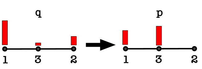
Figure 2: An exploration distribution $p$ derived from $q$ for the game in Eq. 7. The expected loss when playing $p$ is smaller than playing $q$ and simultaneously more information is gained because the third action is revealing.

Optimisation problem

Suppose that exponential weights proposes a distribution $q\in\mathcal{P}$. Our algorithm solves an optimisation problem to find an exploration distribution and estimation function that determine the loss estimators. Given an estimation function $G\in\mathcal{H}$ and outcome $x\in[d]$, define a ‘bias’ function that measures the degree of bias when using importance-weighting to estimate loss differences:

$$\operatorname{bias}_{q}(G;x)=\left\langle q,\,\mathcal{L}e_{x}-\sum_{a=1}^{k}G(a,\Phi_{ax})\right\rangle+\max_{c\in\Pi}\left(\sum_{a=1}^{k}G(a,\Phi_{ax})_{c}-\mathcal{L}_{cx}\right)\,.$$

As a function of $G$ the bias is max-affine and hence convex. It is always non-negative and vanishes when the estimation function $G\in\mathcal{H}_{\circ}$ is unbiased. For $q\in\mathcal{P}$ and $\eta>0$ let $\operatorname{opt}_{q}(\eta)$ be the value of the following convex optimisation problem: $\displaystyle\underset{G\in\mathcal{H},p\in\mathcal{P}}{\text{minimise}}\qquad$ $\displaystyle\max_{x\in[d]}\Bigg{[}\frac{(p-q)^{\top}\mathcal{L}e_{x}+\operatorname{bias}_{q}(G;x)}{\eta}+\frac{1}{\eta^{2}}\sum_{a=1}^{k}p_{a}\Psi_{q}\left(\frac{\eta G(a,\Phi_{ax})}{p_{a}}\right)\Bigg{]}\,.$ (9) We assume that Eq. 9 can be solved exactly to obtain minimising values for $G\in\mathcal{H}$ and $p\in\mathcal{P}$. Our algorithm, however, is robust to small perturbations of these quantities. Numerical issues and a practical approximation are discussed in Appendix F. Let

$$\operatorname{opt}_{*}(\eta)=\sup_{q\in\mathcal{P}}\operatorname{opt}_{q}(\eta)\,.$$

Note that both $\operatorname{opt}_{q}(\eta)$ and $\operatorname{opt}_{*}(\eta)$ depend on $\mathcal{G}$; this dependence is not shown to minimize clutter. The optimisation problem can be formulated as an exponential cone problem and solved using off-the-shelf solvers. The algorithm is a simple combination of exponential weights using the exploration distribution and estimation function provided by solving Eq. 9.

input: $\eta$ for $t=1,\ldots,n$: Compute $\displaystyle Q_{ta}=\frac{\mathds{1}_{\Pi}(a)\exp\left(-\eta\sum_{s=1}^{t-1}\hat{y}_{sa}\right)}{\sum_{b\in\Pi}\exp\left(-\eta\sum_{s=1}^{t-1}\hat{y}_{sb}\right)}$
Solve (9) with $q=Q_{t}$ to find $P_{t}\in\mathcal{P}$ and $G_{t}\in\mathcal{H}$
Sample $A_{t}\sim P_{t}$, observe $\sigma_{t}$ and compute $\displaystyle\hat{y}_{t}=\frac{G_{t}(A_{t},\sigma_{t})}{P_{tA_{t}}}$

Algorithm 1: Exponential weights for partial monitoring with confidence

The regret of Algorithm 1 depends on the learning rate and the value of the optimisation problem, which depends on the structure of the game. Bounds on $\operatorname{opt}_{*}(\eta)$ are provided subsequently.

Theorem 5.

For any $\eta>0$, the regret of Algorithm 1 is bounded by $\displaystyle\mathbb{E}[\mathfrak{R}_{n}]\leq\frac{\log(k)}{\eta}+\eta n\operatorname{opt}_{*}(\eta)$.

Proof.

Let $a^{*}=\operatornamewithlimits{arg\,min}_{a\in[k]}\sum_{t=1}^{n}\mathcal{L}(a,x_{t})$ be the optimal action in hindsight, where ties are broken so that $a^{*}\in\Pi$ is Pareto optimal. Note, this is where we are using that the adversary is oblivious. Then

$$\mathbb{E}[\mathfrak{R}_{n}] =\mathbb{E}\left[\sum_{t=1}^{n}\sum_{b=1}^{k}P_{tb}(\mathcal{L}_{bx_{t}}-\mathcal{L}_{a^{*}x_{t}})\right]$$

$$\leq\mathbb{E}\left[\sum_{t=1}^{n}\left((P_{t}-Q_{t})^{\top}\mathcal{L}e_{x_{t}}+\operatorname{bias}_{Q_{t}}(G_{t};x_{t})\right)\right]+\mathbb{E}\left[\sum_{t=1}^{n}\sum_{b=1}^{k}Q_{tb}(\hat{y}_{tb}-\hat{y}_{ta^{*}})\right]\,.$$ (10)

Next,

$$\mathbb{E}\left[\sum_{t=1}^{n}\sum_{b=1}^{k}Q_{tb}(\hat{y}_{tb}-\hat{y}_{ta^{*}})\right] \leq\frac{\log(k)}{\eta}+\frac{1}{\eta}\mathbb{E}\left[\sum_{t=1}^{n}\Psi_{Q_{t}}(\eta\hat{y}_{t})\right]$$ (11)

$$=\frac{\log(k)}{\eta}+\frac{1}{\eta}\mathbb{E}\left[\sum_{t=1}^{n}\sum_{a=1}^{k}P_{ta}\Psi_{Q_{t}}\!\left(\frac{\eta G_{t}(a,\Phi_{ax_{t}})}{P_{ta}}\right)\right]\,,$$

where Eq. 11 follows from Eq. 5 and the definitions of $Q_{t}$ and $\hat{y}_{t}$. The result follows by combining Eq. 10 and the definition of $\operatorname{opt}_{*}(\eta)$. ∎

Applications

Table 2 provides bounds on $\operatorname{opt}_{*}(\eta)$ for different games and the regret bound that results from optimising the learning rate. The proofs are provided in Sections 5 and 6. Except for locally observable games, they mirror existing proofs bounding the stability of exponential weights. In this way many other results could be added to this table, including bandits with graph feedback [Alon et al.,, 2015] and linear bandits with finitely many arms [Bubeck et al.,, 2012].

Game type	$\text{{opt}}^{\bm{*}}\bm{(\eta)\,}$ bound	Conditions	Ref.	Regret
Bandit	$k/2$		Prop. 8	$\sqrt{2nk\log(k)}$
Full information	$1/2$		Prop. 9	$\sqrt{2n\log(k)}$
Globally observable	$\displaystyle c_{\mathcal{G}}/\sqrt{\eta}$	$\displaystyle\eta\leq 1/c_{\mathcal{G}}^{2}$	Prop. 11	$3(c_{\mathcal{G}}n/2)^{2/3}(\log(k))^{1/3}$
Locally observable non-degenerate	$3k^{3}m^{2}$	$\displaystyle\eta\leq 1/(mk^{2})$	Prop. 12	$2k^{3/2}m\sqrt{3n\log(k)}$

Table 2: Upper bounds on $\operatorname{opt}_{*}(\eta)$ and the regret of Algorithm 1 for different games. The constant $c_{\mathcal{G}}$ is game-dependent and can be exponentially large in $d$, which we believe is unavoidable.

4 Online learning rate tuning

Tuning the learning rate used by Algorithm 1 is delicate. First, it is not clear that $\operatorname{opt}_{*}(\eta)$ can be computed efficiently in general. Second, the learning rate that minimises the bound in Theorem 5 may be overly conservative. Algorithm 2 mitigates these issues by using an adaptive learning rate. The algorithm is parameterised by a constant $B$ that determines the initialisation of the learning rate. $B$ should be chosen large enough that $\eta=1/B$ satisfies the conditions for the relevant game in Table 2, but the additional regret from choosing $B$ too large is only additive.

input: $B$ for $t=1,2,\ldots,$: Set $\displaystyle\eta_{t}=\min\left\{\frac{1}{B},\,\,\sqrt{\frac{\log(k)}{1+\sum_{s=1}^{t-1}V_{s}}}\right\}$
Compute $\displaystyle Q_{ta}=\frac{\mathds{1}_{\Pi}(a)\exp\left(-\eta_{t}\sum_{s=1}^{t-1}\hat{y}_{sa}\right)}{\sum_{b\in\Pi}\exp\left(-\eta_{t}\sum_{s=1}^{t-1}\hat{y}_{sb}\right)}$
Solve (9) with $\eta=\eta_{t}$ and $q=Q_{t}$ to find $V_{t}=\max\{0,\operatorname{opt}_{Q_{t}}(\eta_{t})\}$ and corresponding $P_{t}$ and $G_{t}$
Sample $A_{t}\sim P_{t}$, observe $\sigma_{t}$ and compute $\displaystyle\hat{y}_{t}=\frac{G_{t}(A_{t},\sigma_{t})}{P_{tA_{t}}}$

Algorithm 2: Adaptive exponential weights for partial monitoring

We now present a general theorem that bounds the regret as a function of $(V_{t})_{t}$, which is computed by the algorithm. This theorem implies that Algorithm 2 recovers all regret bounds in Table 2 up to small constant factors and additive terms.

Theorem 6.

There exists a universal constant $c>0$ such that the regret of Algorithm 2 is bounded by

$$\mathbb{E}[\mathfrak{R}_{n}]\leq 5\mathbb{E}\left[\sqrt{\left(1+\sum_{t=1}^{n}V_{t}\right)\log(k)}\right]+\mathbb{E}\left[\max_{t\in[n]}V_{t}\right]\sqrt{\log(k)}+B\log(k)\,.$$

A corollary using the definition of $V_{t}$ is that the regret of Algorithm 2 is bounded by

$$\mathbb{E}[\mathfrak{R}_{n}]=O\left(\sqrt{n\sup\{\max\{0,\operatorname{opt}_{*}(\eta)\}:\eta\leq 1/B\}\log(k)}+B\log(k)\right)\,.$$ (12)

This bound is most useful for full information, bandit and locally observable non-degenerate games when $B$ can be chosen so that $\eta_{1}\leq 1/B$ satisfies the conditions in the second column of Table 2. As a consequence, for games of this category Theorem 6 recovers the bounds in the last column Table 2 up to small constant factors and additive terms.

For games that are globally observable but not locally observable $\operatorname{opt}_{*}(\eta)\to\infty$ as $\eta\to 0$ and the supremum in Eq. 12 is infinite. Soon, we will argue that the learning rate used by Algorithm 2 does not decrease too fast and that the algorithm still achieves the regret bound shown in Table 2 for globally observable games.

Proof sketch of Theorem 6.

We explain only the differences relative to the proof of Theorem 5. Recall that $V_{t}=\max\{0,\operatorname{opt}_{Q_{t}}(\eta_{t})\}$. Note, the learning rate $\eta_{t}$ is non-increasing. Hence, by Eq. 5,

$$\mathbb{E}[\mathfrak{R}_{n}] \leq\mathbb{E}\left[\sum_{t=1}^{n}\sum_{a=1}^{k}Q_{ta}(\hat{y}_{ta}-\hat{y}_{ta^{*}})+\sum_{t=1}^{n}(P_{t}-Q_{t})^{\top}\mathcal{L}e_{x_{t}}+\operatorname{bias}_{Q_{t}}(G_{t};x_{t})\right]$$

$$\leq\mathbb{E}\left[\frac{\log(k)}{\eta_{n}}+\sum_{t=1}^{n}\frac{\Psi_{Q_{t}}(\eta_{t}\hat{y}_{t})}{\eta_{t}}+\sum_{t=1}^{n}(P_{t}-Q_{t})^{\top}\mathcal{L}e_{x_{t}}+\operatorname{bias}_{Q_{t}}(G_{t};x_{t})\right]$$ (13)

$$\leq\mathbb{E}\left[\frac{\log(k)}{\eta_{n}}+\sum_{t=1}^{n}\eta_{t}V_{t}\right]\,,$$ (14)

where Eq. 14 follows from the same argument as the proof of Theorem 5 and the definition of $V_{t}$. The second term is bounded using Lemma 22 in the appendix by

$$\sum_{t=1}^{n}\eta_{t}V_{t} \leq 4\sqrt{\left(1+\frac{1}{2}\sum_{t=1}^{n}V_{t}\right)\log(k)}+\max_{t\in[k]}V_{t}\sqrt{\log(k)}\,.$$

The definition of $(\eta_{t})_{t=1}^{n}$ means that

$$\frac{\log(k)}{\eta_{n}}\leq B\log(k)+\sqrt{\left(1+\sum_{t=1}^{n}V_{t}\right)\log(k)}\,.$$

The bound follows by combining the parts and naive algebra. ∎

As promised, we now show that for sufficiently large $B$ the algorithm achieves the best known regret for any globally observable game.

Proposition 7.

Fix a globally observable game $\mathcal{G}$. Suppose that $\alpha>0$ and $\operatorname{opt}_{*}(\eta)\leq\alpha/\sqrt{\eta}$ for all $\eta\leq 1/B$. Then, the regret of Algorithm 2 on $\mathcal{G}$ is at most

$$\mathbb{E}[\mathfrak{R}_{n}]=O\left((n\alpha)^{2/3}(\log(k))^{1/3}+B\log(k)\right)\,,$$

where the Big-Oh hides only universal constants.

Note that the conditions of this result will be satisfied with $\alpha=c_{\mathcal{G}}$ once $B\geq c_{\mathcal{G}}^{2}$ with (cf. Table 2).

Proof.

The result follows from Theorem 6 and an almost sure bound on $\sum_{t=1}^{n}V_{t}$. Clearly, $\eta_{t}\leq 1/B$ and so by assumption $V_{t}=\max\{0,\operatorname{opt}_{Q_{t}}(\eta_{t})\}\leq\alpha/\sqrt{\eta_{t}}$. Then, using the definition of $(\eta_{t})_{t=1}^{n}$,

$$\frac{\log(k)}{\eta_{t+1}^{2}}\leq\frac{\log(k)}{\eta_{t}^{2}}+\frac{\alpha}{\eta_{t}^{1/2}}=\frac{\log(k)}{\eta_{t}^{2}}+\frac{\alpha}{\log(k)^{1/4}}\left(\frac{\log(k)}{\eta_{t}^{2}}\right)^{\frac{1}{4}}\,.$$

Hence, using the definition of $\eta_{n}$ and Lemma 23 in the appendix,

$$1+\sum_{t=1}^{n}V_{t}\leq\frac{\log(k)}{\eta_{n}^{2}}\leq\left(\frac{3\alpha(n-1)}{4\log(k)^{1/4}}+\max\{1,B^{2}\log(k)\}^{3/4}\right)^{4/3}\,.$$

Substituting the above bound into the dominant term of Theorem 6 shows that

$$\sqrt{\left(1+\sum_{t=1}^{n}V_{t}\right)\log(k)}=O\Big{(}(kn\alpha)^{2/3}(\log(k))^{1/3}+B\log(k)\Big{)}\,.$$

The result is completed by noting that $\max_{t\in[n]}V_{t}\leq\alpha\eta_{n}^{-1/2}$ is lower-order. ∎

5 Bandit, full information and globally observable games

We now bound $\operatorname{opt}_{*}(\eta)$ for bandit, full information and globally observable games. All results follow from the usual arguments for bounding the stability term in the regret guarantee for exponential weights in Eq. 5.

Proposition 8.

For bandit games, $\operatorname{opt}_{*}(\eta)\leq k/2$ for all $\eta>0$.

Proof.

Let $q\in\mathcal{P}$ be arbitrary and let $p=q$ and $G(a,\sigma)=e_{a}\sigma$. This corresponds to the usual importance-weighted estimators used for $k$-armed bandits. Then

$$\operatorname{opt}_{q}(\eta) \leq\max_{x\in[d]}\sum_{a=1}^{k}\frac{p_{a}}{\eta^{2}}\Psi_{q}\left(\frac{\eta G(a,\Phi_{ax})}{p_{a}}\right)=\max_{x\in[d]}\sum_{a=1}^{k}\frac{p_{a}}{\eta^{2}}\Psi_{q}\left(\frac{\eta\mathcal{L}_{ax}e_{a}}{p_{a}}\right)\leq\max_{x\in[d]}\sum_{a=1}^{k}\frac{\mathcal{L}_{ax}^{2}}{2}\leq\frac{k}{2}\,,$$

where in the second last inequality we used Eq. 6 and the fact that $p_{a}=q_{a}$. ∎

Proposition 9.

For full information games, $\operatorname{opt}_{*}(\eta)\leq 1/2$ for all $\eta>0$.

Proof.

As in the previous proof let $p=q$, but now choose $G(a,\sigma)=p_{a}\sigma$, which is unbiased. The argument then follows along the same lines as the proof of Proposition 8. ∎

Remark 10.

You might wonder whether these choices of $p$ and $G$ actually minimise Eq. 9, in which case the algorithm would reduce to Hedge for full information games. As we show in Appendix D, however, they do not. The minimisers of Eq. 9 shift the loss estimates and play a distribution that is close to $q$, but not exactly the same. A similar story holds for bandits.

Proposition 11.

For non-degenerate globally observable games there exists a constant $c_{\mathcal{G}}$ depending only on $\Phi$ and $\mathcal{L}$ such that for all $\eta\leq 1/c_{\mathcal{G}}^{2}$,

$$\operatorname{opt}_{*}(\eta)\leq\frac{c_{\mathcal{G}}}{\sqrt{\eta}}\,.$$

Proof.

By the definition of a globally observable game there exists an unbiased estimation function $G\in\mathcal{H}_{\circ}$. Let $\beta=\left\|G\right\|_{\infty}$ and $c_{\mathcal{G}}=\max\{1,2k\beta\}$. Then let $\gamma=k\beta\sqrt{\eta}$ and $p=(1-\gamma)q+\gamma\bm{1}/k$, which is a probability distribution since $\gamma\in[0,1]$ for $\eta\leq 1/c_{\mathcal{G}}^{2}$. We claim that $\eta G(a,\Phi_{ax})/p_{a}\geq-\bm{1}$, which follows from the definitions of $\gamma$ and $\beta$ so that

$$p_{a}\bm{1}\geq\frac{\gamma}{k}\bm{1}=\beta\sqrt{\eta}\bm{1}\geq\beta\eta\bm{1}\geq\eta G(a,\Phi_{ax})\,,$$

where the second inequality uses the fact that $c_{\mathcal{G}}\geq 1$ and $\eta\leq 1/c_{\mathcal{G}}^{2}\leq 1$. To bound the objective notice that for any $x\in[d]$ it holds that

$$\frac{1}{\eta}(p-q)^{\top}\mathcal{L}e_{x}=\frac{\gamma}{\eta}(\bm{1}/k-q)^{\top}\mathcal{L}e_{x}\leq\frac{\gamma}{\eta}=\frac{k\beta}{\sqrt{\eta}}\,.$$

For the second term in the objective, by Eq. 6,

$$\frac{1}{\eta^{2}}\max_{x\in[d]}\sum_{a=1}^{k}p_{a}\Psi_{q}\left(\frac{\eta G(a,\Phi_{ax})}{p_{a}}\right) \leq\max_{x\in[d]}\sum_{a=1}^{k}\frac{\left\|G(a,\Phi_{ax})\right\|_{\operatorname{diag}(q)}^{2}}{p_{a}}$$

$$\leq\frac{k}{\gamma}\max_{x\in[d]}\sum_{a=1}^{k}\langle q,G(a,\Phi_{ax})^{2}\rangle$$

$$\leq\frac{k^{2}\beta^{2}}{\gamma}=\frac{k\beta}{\sqrt{\eta}}\,.$$

The result follows by combining the previous two displays and the definition of $c_{\mathcal{G}}$. ∎

6 Locally observable games

Controlling $\operatorname{opt}_{*}(\eta)$ for locally observable games is more involved. The main result of this section is a proof of the following proposition.

Proposition 12.

For locally observable non-degenerate games and $\eta\leq 1/(2mk^{2})$,

$$\operatorname{opt}_{*}(\eta)\leq 3m^{2}k^{3}\,.$$

We make use of the water transfer operator, which is a construction from our earlier paper that provides an exploration distribution suitable for locally observable games in the Bayesian setting. The challenge in partial monitoring is that the observability structure only allows for pairwise comparison between neighbours. This is problematic when two non-neighbouring actions are played with high probability and the actions separating them are played with low probability. Given distributions $q\in\mathcal{P}$ and $\nu\in\mathcal{D}$, the water transfer operator ‘flows’ probability in $q$ towards the greedy action $a$ for which $\nu\in C_{a}$. Then all loss differences can be estimated relative to the greedy action. This decreases the variance of estimation without increasing the expected loss when the adversary samples its action from $\nu$.

Lemma 13 (Lattimore and Szepesvári, 2019b ).

Suppose that $\mathcal{G}$ is non-degenerate and locally observable and $\nu\in\mathcal{D}$. Then there exists a function $W_{\nu}:\mathcal{P}\to\mathcal{P}$ such that the following hold for all $q\in\mathcal{P}$:

1. The expected loss does not increase: $\left(W_{\nu}(q)-q\right)^{\top}\mathcal{L}\nu\leq 0$.

2. Action probabilities are not too small: $W_{\nu}(q)_{a}\geq q_{a}/k$ for all $a\in[k]$.

3. Probabilities increase towards the root of some in-tree: there exists an in-tree $\mathcal{T}\subseteq\mathcal{E}$ over $[k]$ such that $W_{\nu}(q)_{a}\leq W_{\nu}(q)_{b}$ for all $(a,b)\in\mathcal{T}$.

A simplified proof of the above lemma is provided for completeness in Appendix B.

Proof of Proposition 12.

Let $q\in\mathcal{P}$. By Sion’s minimax theorem

$$\operatorname{opt}_{q}(\eta) \leq\min_{G\in\mathcal{H}_{\circ},p\in\mathcal{P}}\max_{\nu\in\mathcal{D}}\left[\frac{1}{\eta}(p-q)^{\top}\mathcal{L}\nu+\frac{1}{\eta^{2}}\sum_{x=1}^{d}\nu_{x}\sum_{a=1}^{k}p_{a}\Psi_{q}\left(\frac{\eta G(a,\Phi_{ax})}{p_{a}}\right)\right]$$

$$=\max_{\nu\in\mathcal{D}}\min_{G\in\mathcal{H}_{\circ},p\in\mathcal{P}}\left[\frac{1}{\eta}(p-q)^{\top}\mathcal{L}\nu+\frac{1}{\eta^{2}}\sum_{x=1}^{d}\nu_{x}\sum_{a=1}^{k}p_{a}\Psi_{q}\left(\frac{\eta G(a,\Phi_{ax})}{p_{a}}\right)\right]\,,$$

where in the first inequality we added the constraint that $G\in\mathcal{H}_{\circ}$, which zeros the bias term. Let $\nu\in\mathcal{D}$ and let $\mathcal{T}$ and $r=W_{\nu}(q)$ be the in-tree over $[k]$ and distribution in $\mathcal{P}$ provided by the water transfer operator (Lemma 13), respectively. Define $G\in\mathcal{H}_{\circ}$ by

$$G(a,\sigma)_{b}=\sum_{e\in\operatorname{path}_{\mathcal{T}}(b)}w_{e}(a,\sigma)\,.$$

By Lemma 20 and the assumption that $\mathcal{G}$ is non-degenerate, $w_{e}$ can be chosen so that $\left\|w_{e}\right\|_{\infty}\leq m/2$. Since paths in $\mathcal{T}$ have length at most $k$ it follows that

$$\left\|G\right\|_{\infty}\leq km/2\,.$$

Furthermore, $G\in\mathcal{H}_{\circ}$ by the proof of Lemma 4. Then let $\gamma=\eta mk^{2}/2$ and $p=(1-\gamma)r+\gamma\bm{1}/k$, which means that for any $x\in[d]$,

$$\frac{\eta G(a,\Phi_{ax})}{p_{a}}\geq-\frac{\eta mk^{2}}{2\gamma}=-1\,.$$

Additionally, the assumption that $\eta\leq 1/(mk^{2})$ means that $\gamma\leq 1/2$ so that $r\geq p/2$. Hence, by Eq. 6 and using Parts (b) and (c) of Lemma 13 with the definition of $r$,

$$\frac{1}{\eta^{2}}\sum_{a=1}^{k}p_{a}\Psi_{q}\left(\frac{\eta G(a,\Phi_{ax})}{p_{a}}\right) \leq\sum_{a=1}^{k}\frac{\left\|G(a,\Phi_{ax})\right\|^{2}_{\operatorname{diag}(q)}}{p_{a}}$$

$$\leq 2\sum_{a=1}^{k}\frac{\left\|G(a,\Phi_{ax})\right\|^{2}_{\operatorname{diag}(q)}}{r_{a}}$$

$$=2\sum_{b=1}^{k}\sum_{a=1}^{k}\frac{q_{b}}{r_{a}}\left(\sum_{e\in\operatorname{path}_{\mathcal{T}}(b)}w_{e}(a,\Phi_{ax})\right)^{2}$$

$$\leq\frac{m^{2}}{2}\sum_{b=1}^{k}\sum_{a=1}^{k}\frac{q_{b}}{r_{a}}\left(\sum_{e\in\operatorname{path}_{\mathcal{T}}(b)}\mathds{1}(a\in e)\right)^{2}$$

$$\leq 2k^{3}m^{2}\,,$$

where we used Part (b) of Lemma 13 to show that $q_{b}\leq kr_{b}$ and Part (c) to show that $r_{a}\geq r_{b}$ for $a\in\operatorname{path}_{\mathcal{T}}(b)$. Finally,

$$\frac{1}{\eta}(p-q)^{\top}\mathcal{L}\nu =\frac{1}{\eta}(r-q)^{\top}\mathcal{L}\nu+\frac{\gamma}{\eta}(\bm{1}/k-r)^{\top}\mathcal{L}\nu\leq\frac{\gamma}{\eta}(\bm{1}/k-r)^{\top}\mathcal{L}\nu\leq\frac{\gamma}{\gamma}=mk^{2}\leq k^{3}m^{2}\,.$$

Hence $\operatorname{opt}_{q}(\eta)\leq 3k^{3}m^{2}$. ∎

Remark 14.

The bound can be improved to $\operatorname{opt}_{q}(\eta)\leq 3km^{2}\operatorname{diam}(\mathcal{E})^{2}$, where $\operatorname{diam}(\mathcal{E})$ is the diameter of the neighbourhood graph.

7 Discussion

We introduced a new algorithm for finite partial monitoring that is efficient, nearly parameter free and enjoys roughly the best known regret in all classes of games. Notably, this is the first efficient algorithm for which the regret is independent of arbitrarily large game-dependent constants for locally observable non-degenerate games. A natural criticism of previous algorithms for partial monitoring is that the algorithms are generally quite conservative and not practical for normal problems. As far as we can tell, the proposed algorithm does not suffer from this problem, at least recovering standard bounds in bandit and full information settings. In certain cases the algorithm may also adapt to the choices of the adversary. The principle for finding an exploration distribution and estimation procedure is generic and may work well in other problems.

Lower bounds

The best known lower bound for locally observable partial monitoring games is either $\Omega(\sqrt{kn})$ or $\Omega(d\sqrt{n})$, which are witnessed by a standard Bernoulli bandit [Auer et al.,, 1995] and a result by the authors [Lattimore and Szepesvári, 2019a, ]. If pressed, we would speculate that $\Theta(d\sqrt{kn})$ is the correct worst-case regret over all $d$-outcome $k$-action non-degenerate locally observable partial monitoring games, at least as $n$ tends to infinity.

High probability bounds

By replacing the bias term in Eq. 9 with a constraint on a certain moment-generating function the algorithm can be adapted to prove high probability bounds. Details are provided in Appendix A.

Infinite outcome spaces

Finiteness of the outcome space was not used in the proofs of Theorem 5 or Theorem 6 and in particular the results in Table 2 continue to hold in this case The main cost of infinite outcome spaces is that the optimisation problem Eq. 9 is unlikely to be tractable without additional structure. Classic examples of infinite games for which the regret can be well controlled are bandit and full information games. In both games the outcomes $(x_{t})_{t=1}^{n}$ are chosen in $\mathcal{X}=[0,1]^{k}$ and $\mathcal{L}(a,x)=x_{a}$ (using the notation of Remark 1). The signal function is $\Phi(a,x)=x_{a}$ for bandits and $\Phi(a,x)=x$ for the full information games. Exploring the existence of a simple classification theorem for infinite-outcome games is an interesting future direction. Understanding when Eq. 9 is tractable is also intriguing.

Game-dependent bounds

One of the objectives of this work was to design an efficient algorithm for which the regret does not depend on arbitrarily large game-dependent constants. Naturally it is desirable to have small game-dependent constants and adaptivity to the choices of the adversary. Table 2 provides upper bounds on $\operatorname{opt}_{*}(\eta)$ for various classes, but the actual values depends on the game. Understanding the dependence of this optimisation problem on the structure of the loss and signal matrices is an interesting open direction. Also interesting is whether or not $\operatorname{opt}_{*}(\eta)$ is a fundamental quantity for the difficulty of the game and/or the regret of our algorithms.

Adaptivity

Algorithm 2 already exhibits some adaptivity in the lucky situation that $V_{t}$ is small. This is not entirely satisfactory, however, since $V_{t}$ is a random variable that depends on the choices of both the learner and the adversary. We anticipate that all the usual enhancements for adaptivity – log barrier, biased estimates and optimism – can be applied here [Rakhlin and Sridharan,, 2013; Bubeck et al.,, 2018; Wei and Luo,, 2018; Bubeck et al.,, 2019, for example]. A related challenge would be to seek a best-of-both-worlds result, perhaps using the INF potential [Zimmert et al.,, 2019].

Beyond exponential weights

The objective in Eq. 9 is chosen so that the terms in Eq. 11 are well controlled, which corresponds to bounding the stability term in the regret analysis of exponential weights. Other algorithms can be obtained by replacing exponential weights with follow the regularized leader and Legendre potential $F$. A standard regret bound (holding under certain technical conditions) is

$$\mathbb{E}[\mathfrak{R}_{n}] \leq\frac{\operatorname{diam}_{F}(\mathcal{P})}{\eta}+\frac{1}{\eta}\mathbb{E}\left[\sum_{t=1}^{n}\sum_{a=1}^{k}P_{ta}D_{F^{*}}\left(\nabla F(Q_{t})-\frac{\eta G_{t}(a,\Phi_{ax_{t}})}{P_{ta}},\nabla F(Q_{t})\right)\right]$$ (15)

$$\qquad\qquad\qquad\qquad\qquad+\mathbb{E}\left[\sum_{t=1}^{n}(P_{t}-Q_{t})^{\top}\mathcal{L}e_{x_{t}}+\operatorname{bias}_{Q_{t}}(G_{t};x_{t})\right]\,.$$

where $\operatorname{diam}_{F}(\mathcal{P})=\max_{x,y\in\mathcal{P}}F(x)-F(y)$ is the diameter and $D_{F^{*}}(x,y)$ is the Bregman divergence between $x$ and $y$ with respect to the Fenchel conjugate of $F$. Let

$$\Psi_{q}(z)=D_{F^{*}}(\nabla F(q)-z,\nabla F(q))\,.$$

Then convexity of $F^{*}$ implies that the perspective $(p,z)\mapsto p\Psi_{q}(z/p)$ is also convex for $p>0$. When $F$ is the unnormalised negentropy, the definition above reduces to Eq. 4. All this means that the same approach holds more broadly for other potentials, which carry certain advantages in some settings [Audibert and Bubeck,, 2009; Bubeck et al.,, 2018; Wei and Luo,, 2018; Bubeck et al.,, 2019, and others]. For more details on follow the regularised leader and bounds of the form in Eq. 15, see [Lattimore and Szepesvári,, 2019, Chapter 28] and [Hazan,, 2016]. We leave a deeper exploration of these ideas for the future.

Degenerate games

The non-degeneracy assumption is purely for simplicity. Only the proof of Proposition 12 and its dependents need to be modified in minor ways. The notable difference is that the magnitude of the estimation vectors is no longer guaranteed to be small. More specifically, Lemma 20 does not hold when estimating loss differences between actions $(a,b)$ for which there are degenerate actions $c$ with $C_{c}=C_{a}\cap C_{b}$. As in our previous work, using Proposition 21 instead introduces constants that may be exponential in $d$, which we believe is unavoidable [Lattimore and Szepesvári, 2019b, ]. Duplicate actions can be handled similarly and have the same affect.

Connections between stability and the information ratio

Zimmert and Lattimore, [2019] have shown that the generalised information ratio can be bounded by a worst-case bound on the stability term of mirror descent, which makes a connection between the information-theoretic tools and those from online convex optimisation. Here we work in the other direction, using duality and the techniques for bounding the information ratio to bound the stability term. The argument does not provide an equivalence between stability and the information ratio, but perhaps reinforces the feeling that there is an interesting connection here.

Acknowledgements

We are grateful to András György for many insightful comments.

Appendix A High probability bounds

The same design principle can be used to construct algorithms for which the regret is controlled with high probability. The idea is to replace the bias term in the objective with constraints on the range of the loss estimators and on an appropriately chosen moment-generating function. Given $q\in\mathcal{P}$ and $\eta>0$, let $\operatorname{opthp}_{q}(\eta)$ be the solution to the following optimisation problem:

$\displaystyle\underset{G\in\mathcal{H},p\in\mathcal{P},\,\lambda\geq 0}{\text{minimise}}\qquad$ $\displaystyle\lambda+\frac{2}{\eta^{2}}\max_{x\in[d]}\sum_{a=1}^{k}p_{a}\Psi_{q}\left(\frac{\eta G(a,\Phi_{ax})}{p_{a}}\right)$ (16) subject to $\displaystyle\max_{c\in[k]}\sum_{a=1}^{k}p_{a}\exp\left(\eta\left(\mathcal{L}_{ax}-\mathcal{L}_{cx}-\frac{\langle q-e_{c},\,G(a,\Phi_{ax})\rangle}{p_{a}}\right)\right)\leq\exp(\lambda\eta^{2})$ and $\displaystyle\eta\left\|G(a,\sigma)\right\|_{\infty}\leq p_{a}\text{ for all $a$ and $\sigma$}\,.$

The optimisation problem in Eq. 16 is not convex, but the solution can be approximated efficiently within a factor of two. Let $\operatorname{opthp}_{q}(\eta,\lambda)$ be the optimal value of Eq. 16 with a fixed value of $\lambda$, which is convex. A larger value of $\lambda$ leads to a larger constraint set and hence $\lambda\mapsto\operatorname{opthp}_{q}(\eta,\lambda)-\lambda$ is decreasing. Then the bisection method can be used to find (approximately) the value of $\lambda$ such that $\operatorname{opthp}_{q}(\eta,\lambda)=2\lambda$ and you can check that for this choice $\operatorname{opthp}_{q}(\eta,\lambda)\leq 2\operatorname{opthp}_{q}(\eta)$. We also define

$$\operatorname{opthp}_{*}(\eta) =\sup_{q\in\mathcal{P}}\operatorname{opthp}_{q}(\eta)\,.$$

The algorithm is exactly the same as Algorithm 1 except that the optimisation problem in Eq. 16 is used instead of Eq. 9.

input: $\eta$ for $t=1,\ldots,n$: Compute $\displaystyle Q_{ta}=\frac{\mathds{1}_{\Pi}(a)\exp\left(-\eta\sum_{s=1}^{t-1}\hat{y}_{sa}\right)}{\sum_{b\in\Pi}\exp\left(-\eta\sum_{s=1}^{t-1}\hat{y}_{sb}\right)}$
Solve (16) with $q=Q_{t}$ to find $\lambda_{t}\in\mathbb{R}$ and $P_{t}\in\mathcal{P}$ and $G_{t}\in\mathcal{H}$
Sample $A_{t}\sim P_{t}$ and observe $\sigma_{t}$
Compute $\displaystyle\hat{y}_{t}=\frac{G_{t}(A_{t},\sigma_{t})}{P_{tA_{t}}}$

Algorithm 3: Exponential weights for partial monitoring

Theorem 15.

With probability at least $1-2\delta$ the regret of Algorithm 3 is bounded by

$$\mathfrak{R}_{n}\leq\frac{\log(k)+2\log(1/\delta)}{\eta}+\eta n\operatorname{opthp}_{*}(\eta)\,.$$

Proof.

Let $(\lambda_{t})_{t=1}^{n}$ be the sequence of real values as defined in the algorithm. Using Lemma 26, the regret is bounded with probability at least $1-\delta$ by

$$\mathfrak{R}_{n} =\sum_{t=1}^{n}\left(\mathcal{L}_{A_{t}x_{t}}-\mathcal{L}_{a^{*}x_{t}}\right)\leq\frac{\log(1/\delta)}{\eta}+\eta\sum_{t=1}^{n}\lambda_{t}+\sum_{t=1}^{n}\sum_{b=1}^{k}Q_{tb}\left(\hat{y}_{tb}-\hat{y}_{ta^{*}}\right)\,.$$

The second sum is bounded as in the proof of Theorem 5 using Eq. 5 by

$$\sum_{t=1}^{n}\sum_{b=1}^{k}Q_{tb}\left(\hat{y}_{tb}-\hat{y}_{ta^{*}}\right) \leq\frac{\log(k)}{\eta}+\frac{1}{\eta}\sum_{t=1}^{n}\Psi_{q}\left(\eta\hat{y}_{t}\right)\,.$$

Let $\mathbb{E}_{t-1}[\cdot]$ denote the expectation conditioned on the history observed after $t-1$ rounds. The last constraint in Eq. 16 ensure that $|\eta\hat{y}_{t}|\leq 1$. Therefore $\Psi_{q}(\eta\hat{y}_{t})\in[0,1]$ and

$$\mathbb{E}_{t-1}\left[\exp\big{(}\Psi_{Q_{t}}(\eta\hat{y}_{t})-\mathbb{E}_{t-1}[\Psi_{Q_{t}}(\eta\hat{y}_{t})]\big{)}\right] \leq 1+\mathbb{E}_{t-1}\left[(\Psi_{Q_{t}}(\eta\hat{y}_{t}))^{2}\right]\leq\exp\left(\mathbb{E}_{t-1}\left[\Psi_{Q_{t}}(\eta\hat{y}_{t})\right]\right)\,,$$

where we used that $\exp(x)\leq 1+x+x^{2}$ for $x\leq 1$ and that $\mathbb{E}[X^{2}]\leq\mathbb{E}[X]$ for random variables $X\in[0,1]$ and finally that $1+x\leq\exp(x)$. Hence, another application of Lemma 26 shows that with probability at least $1-\delta$,

$$\frac{1}{\eta}\sum_{t=1}^{n}\Psi_{Q_{t}}\left(\eta\hat{y}_{t}\right) \leq\frac{2}{\eta}\sum_{t=1}^{n}\mathbb{E}_{t-1}\left[\Psi_{Q_{t}}\left(\eta\hat{y}_{t}\right)\right]+\frac{1}{\eta}\log\left(\frac{1}{\delta}\right)$$

$$\leq\eta\sum_{t=1}^{n}\left(\operatorname{opthp}_{Q_{t}}(\eta)-\lambda_{t}\right)+\frac{1}{\eta}\log\left(\frac{1}{\delta}\right)\,.$$

Combining the pieces shows that the regret is bounded with probability at least $1-2\delta$ by

$$\mathfrak{R}_{n} \leq\frac{\log(k)+2\log(1/\delta)}{\eta}+\eta\sum_{t=1}^{n}\operatorname{opthp}_{Q_{t}}(\eta)\leq\frac{\log(k)+2\log(1/\delta)}{\eta}+\eta n\operatorname{opthp}_{*}(\eta)\,.\qed$$

Remark 16.

Algorithm 3 can be modified with a little effort to adapt the learning rate in a similar manner as Algorithm 2. The analysis remains more-or-less the same except a version of Lemma 26 must be proven for decreasing sequences of learning rates.

Applications

Like $\operatorname{opt}_{q}(\eta)$, the quantity $\operatorname{opthp}_{q}(\eta)$ is game-dependent. In all the applications that we know of the stability component of the optimisation problem in Eq. 9 can be bounding by choosing $p$ and $G$ so that the loss estimators do not have magnitude larger than $1/\eta$ and then using the bounds on $\Psi_{q}$ in Eq. 6. The following lemma extracts the core assumptions needed for this argument. Afterwards we give applications for full information, bandit and partial monitoring games.

Lemma 17.

Let $q\in\mathcal{P}$ and $\eta\in(0,1/2)$ and suppose there exists a $p\in\mathcal{P}$ and $G\in\mathcal{H}_{\circ}$ and $\varphi\in\mathbb{R}^{k}$ with $\varphi\geq\bm{0}$ such that for all actions $a$ and $b$ and outcomes $x$,

$$\frac{\eta}{p_{a}}\left\|G(a,\Phi_{ax})\right\|_{\infty}\leq\frac{1}{2}\qquad\text{and}\qquad\sum_{a=1}^{k}\frac{G(a,\Phi_{ax})^{2}}{p_{a}}\leq\varphi\qquad\text{and}\qquad\eta^{2}\varphi\leq\frac{\bm{1}}{2}\,.$$ (17)

Then $\operatorname{opthp}_{q}(\eta)\leq 1+12\langle q,\varphi\rangle+\frac{1}{\eta}\max_{x\in[d]}(p-q)^{\top}\mathcal{L}e_{x}$.

Proof.

Let $G^{\prime}(a,\sigma)=G(a,\sigma)-3\eta p_{a}\varphi$. At heart this is the same biased loss estimator used by Auer et al., [1995] and generalised by Abernethy and Rakhlin, [2009]. Define

$$\lambda=1+6\langle q,\varphi\rangle+\frac{1}{\eta}\max_{x\in[d]}(p-q)\mathcal{L}e_{x}\,.$$

We now show that $G^{\prime}$, $p$ and $\lambda$ satisfies the constraints in Eq. 16 and then that they provide a witness to the claimed upper bound on $\operatorname{opthp}_{q}$. For any action $c$ and outcome $x$,

$$\sum_{a=1}^{k}p_{a}\exp\left(\eta\left(\mathcal{L}_{ax}-\mathcal{L}_{cx}-\frac{\langle q-e_{c},G^{\prime}(a,\Phi_{ax})\rangle}{p_{a}}\right)\right)$$

$$\qquad=\exp\left(3\eta^{2}\langle q-e_{c},\varphi\rangle-\eta\mathcal{L}_{cx}\right)\sum_{a=1}^{k}p_{a}\exp\left(\eta\left(\mathcal{L}_{ax}-\frac{\langle q-e_{c},G(a,\Phi_{ax})\rangle}{p_{a}}\right)\right)\,.$$ (18)

The second term is bounded using $\exp(x)\leq 1+x+x^{2}$ for $x\leq 1$,

$$\sum_{a=1}^{k}p_{a}\exp\left(\eta\left(\mathcal{L}_{ax}-\frac{\langle q-e_{c},G(a,\Phi_{ax})\rangle}{p_{a}}\right)\right)$$

$$\qquad\leq 1+\eta\mathcal{L}_{cx}+\eta(p-q)^{\top}\mathcal{L}e_{x}+\eta^{2}\sum_{a=1}^{k}p_{a}\left(\mathcal{L}_{ax}-\frac{\langle q-e_{c},G(a,\Phi_{ax})\rangle}{p_{a}}\right)^{2}$$

$$\qquad\leq 1+\eta\mathcal{L}_{cx}+\eta(p-q)^{\top}\mathcal{L}e_{x}+3\eta^{2}\left(1+\sum_{a=1}^{k}\frac{\langle q,G(a,\Phi_{ax})^{2}\rangle}{p_{a}}+\sum_{a=1}^{k}\frac{\langle e_{c},G(a,\Phi_{ax})^{2}\rangle}{p_{a}}\right)$$

$$\qquad\leq\exp\left(\eta\mathcal{L}_{cx}+\eta(p-q)^{\top}\mathcal{L}e_{x}+3\eta^{2}(1+\langle q+e_{c},\varphi\rangle)\right)\,,$$

where in the first inequality we used the fact that $G\in\mathcal{H}_{\circ}$ is unbiased. In the second we used that $(x+y+z)^{2}\leq 3x^{2}+3y^{2}+3z^{2}$. In the last we used the assumptions on $\varphi$ and $1+x\leq\exp(x)$. Combining with Eq. 18 shows that

$$\sum_{a=1}^{k}p_{a}\exp\left(\eta\left(\mathcal{L}_{ax}-\mathcal{L}_{cx}-\frac{\langle q-e_{c},G^{\prime}(a,\Phi_{ax})\rangle}{p_{a}}\right)\right)\leq\exp(\lambda\eta^{2})\,,$$

which confirms that the first constraint in Eq. 16 is satisfies for this choice of $G$ and $p$. The second constraint in Eq. 16 is satisfied from the assumptions of the lemma:

$$\frac{\eta}{p_{a}}\left\|G^{\prime}(a,\sigma)\right\|_{\infty}\leq\frac{\eta}{p_{a}}\left\|G(a,\sigma)\right\|_{\infty}+\eta^{2}\left\|\varphi\right\|_{\infty}\leq 1\,.$$

For the objective we have

$$\lambda+\frac{2}{\eta^{2}}\sum_{a=1}^{k}p_{a}\Psi_{q}\left(\frac{\eta G^{\prime}(a,\Phi_{ax})}{p_{a}}\right) \leq\lambda+2\sum_{a=1}^{k}\frac{\langle q,G^{\prime}(a,\Phi_{ax})^{2}\rangle}{p_{a}}$$

$$\leq\lambda+4\sum_{a=1}^{k}\frac{\langle q,G(a,\Phi_{ax})^{2}\rangle}{p_{a}}+4\eta^{2}\langle q,\varphi^{2}\rangle$$

$$\leq\lambda+6\langle q,\varphi\rangle$$

$$=1+12\langle q,\varphi\rangle+\frac{1}{\eta}\max_{x\in[d]}(p-q)^{\top}\mathcal{L}e_{x}\,.\qed$$

Using the same analysis as in the proofs of Propositions 9, 8, 12 and 11 you can prove all the bounds in Table 3. For example, Lemma 17 can be applied to full information games by defining $G(a,\sigma)=p_{a}\sigma$ and $p=q$ and $\varphi=\bm{1}$. Then $\langle q,\varphi\rangle=1$ and for $\eta\leq 1/2$ it follows that $\operatorname{opthp}_{*}(\eta)\leq 13$. And hence the familiar bound of $O(\sqrt{n\log(k/\delta)})$ is recovered using Theorem 15. For bandits choose $G(a,\sigma)=e_{a}\sigma$ and $p=(1-\gamma)q+\gamma\bm{1}/k$ with $\gamma=k\eta$ and $\varphi=1/p$. Then $\operatorname{opthp}_{*}(\eta)\leq 1+13k$ and the regret is $O(\sqrt{nk\log(k/\delta)})$ as expected.

Remark 18.

The bounds in Table 3 are obtained by tuning the learning rate in a manner that depends on $\delta$. The learning rate can be tuned without the knowledge of $\delta$, but then the dependence on $\log(1/\delta)$ moves outside the square root, a price that is known to be unavoidable [Gerchinovitz and Lattimore,, 2016].

Game type	Regret
Full information	$O\left(\sqrt{n\log(k/\delta)}\right)$
Bandit	$O\left(\sqrt{nk\log(k/\delta)}\right)$
Globally observable	$O\left((c_{\mathcal{G}}n)^{2/3}\log(k/\delta)^{1/3}\right)$
Locally observable non-degenerate	$O\left(mk^{3/2}\sqrt{n\log(k/\delta)}\right)$

Table 3: High probability regret upper bounds that hold for a given $\delta\in(0,1)$. The constant $c_{\mathcal{G}}$ is game-dependent and can be exponentially large in $d$, which we believe is unavoidable.

Appendix B Water transfer operator

Here we provide a simple proof of Lemma 13. Let $\mathcal{T}$ be an in-tree over $[k]$. A vector $y\in\mathbb{R}^{k}$ is called $\mathcal{T}$-increasing if $y_{a}\leq y_{b}$ for all $(a,b)\in\mathcal{T}$, which means the function $a\mapsto y_{a}$ is increasing towards the root of $\mathcal{T}$. Similarly, $y$ is $\mathcal{T}$-decreasing if $y_{a}\geq y_{b}$ for all $(a,b)\in\mathcal{T}$.

Lemma 19.

Given a tree $\mathcal{T}$ over $[k]$ and $q\in\mathcal{P}$, there exists an $r\in\mathcal{P}$ such that:

1. $r\geq q/k$.

2. $r$ is $\mathcal{T}$-increasing.

3. $\langle r-q,y\rangle\leq 0$ for all $\mathcal{T}$-decreasing $y\in\mathbb{R}^{k}$.

Proof.

Let $\operatorname{desc}_{\mathcal{T}}(a)$ be the descendants of $a$ in $\mathcal{T}$ with the convention that $a\in\operatorname{desc}_{\mathcal{T}}(a)$. Define $d_{\mathcal{T}}(a)$ as the depth of $a$ in $\mathcal{T}$ with $d_{\mathcal{T}}(\operatorname{root}_{\mathcal{T}})=1$. Define $r_{a}=\sum_{b\in\operatorname{desc}_{\mathcal{T}}(a)}q_{b}/d_{\mathcal{T}}(b)$, which is illustrated in Fig. 3. That $r\in\mathcal{P}$ follows since

$$\sum_{a=1}^{k}\sum_{b\in\operatorname{desc}_{\mathcal{T}}(a)}\frac{q_{b}}{d_{\mathcal{T}}(b)} =\sum_{b=1}^{k}\frac{q_{b}}{d_{\mathcal{T}}(b)}\sum_{a=1}^{k}\mathds{1}(b\in\operatorname{desc}_{\mathcal{T}}(a))=\sum_{b=1}^{k}q_{b}=1\,.$$

Part (a) follows because $d_{\mathcal{T}}(b)\leq k$. Part (b) follows because if $(a,b)\in\mathcal{T}$, then $\operatorname{desc}_{\mathcal{T}}(a)\subset\operatorname{desc}_{\mathcal{T}}(b)$. For the last part, the fact that $y$ is $\mathcal{T}$-decreasing means that

$$\langle r,y\rangle =\sum_{a=1}^{k}y_{a}\sum_{b\in\operatorname{desc}_{\mathcal{T}}(a)}\frac{q_{b}}{d_{\mathcal{T}}(b)}\leq\sum_{a=1}^{k}\sum_{b\in\operatorname{desc}_{\mathcal{T}}(a)}\frac{y_{b}q_{b}}{d_{\mathcal{T}}(b)}=\sum_{b=1}^{k}\frac{y_{b}q_{b}}{d_{\mathcal{T}(b)}}\sum_{a=1}^{k}\mathds{1}(b\in\operatorname{desc}_{\mathcal{T}}(a))=\langle q,y\rangle\,.$$

Rearranging completes the proof. ∎

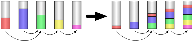
Figure 3: Illustration of $r$ as defined in the proof of Lemma 13.

Proof of Lemma 13.

The result follows from Lemma 19 and by proving there exists an in-tree $\mathcal{T}$ over $[k]$ such that $\mathcal{L}\nu$ is $\mathcal{T}$-decreasing. We start by proving the existence of $\mathcal{T}$ when $\nu\in\operatorname{ri}(C_{a^{*}_{\nu}})$ for some Parent optimal action $a^{*}_{\nu}$. Define a function $\operatorname{par}:[k]\to[k]$ by

$$\operatorname{par}(a)=\operatornamewithlimits{arg\,min}_{b:(a,b)\in\mathcal{E}}e_{b}^{\top}\mathcal{L}\nu\,,$$

where the ties in the $\operatornamewithlimits{arg\,min}$ are broken arbitrarily. We will shortly show that $(e_{a}-e_{\operatorname{par}(a)})^{\top}\mathcal{L}\nu>0$ for all $a\neq a^{*}_{\nu}$, which means that $\mathcal{T}=\{(a,\operatorname{par}(a)):a\neq a^{*}_{\nu}\}$ is an in-tree over $[k]$ on which $\mathcal{L}^{\top}\nu$ is $\mathcal{T}$-decreasing. Let $D=\{(a,b,c):\dim(C_{a}\cap C_{b}\cap C_{c})\leq d-3\}$ and

$$A=\bigcup_{a,b,c\in D}C_{a}\cap C_{b}\cap C_{c}\,.$$

Let $a\neq a^{*}_{\nu}$ and $\mu\in\operatorname{ri}(C_{a})$ be such that the chord connecting $\mu$ and $\nu$ does not intersect $A$. Next, let $\rho\in\partial C_{a}$ be such that $\rho-\mu$ is proportional to $\nu-\mu$ and $b\neq a$ be an action with $\rho\in C_{b}$. Since $\mu\in\operatorname{ri}(C_{a})$ we have $e_{a}^{\top}\mathcal{L}\mu<e_{b}^{\top}\mathcal{L}\mu$ and since $\rho\in C_{a}\cap C_{b}$ we have $e_{a}^{\top}\mathcal{L}\rho=e_{b}^{\top}\mathcal{L}\rho$. Hence $e_{b}^{\top}\mathcal{L}\nu<e_{a}^{\top}\mathcal{L}\nu$. The choice of $\mu$ ensures that $\rho\notin A$ and hence $(a,b)\in\mathcal{E}$, which means that $\operatorname{par}(a)$ is well defined and satisfies the claimed monotonicity conditions. Suppose now that $\nu$ is arbitrary and $a^{*}_{\nu}\in C_{\nu}$. Then take a sequence $(\nu_{t})_{t=1}^{\infty}$ converging to $\nu$ and with $\nu_{t}\in\operatorname{ri}(a^{*}_{\nu})$. By the previous argument there exists a sequence of in-trees $(\mathcal{T}_{t})_{t=1}^{\infty}$ such that $\mathcal{L}\nu_{t}$ is $\mathcal{T}_{t}$-decreasing. Since the space of trees is finite, the sequence $(\mathcal{T}_{t})_{t=1}^{\infty}$ has a cluster point $\mathcal{T}$ and it is easy to see that $\mathcal{L}\nu$ is $\mathcal{T}$-decreasing. ∎

Appendix C Bounds on the estimation functions

The polynomial dependence on $k$ and $m$ in locally observable non-degenerate games follows from the simple combinatorial structure when loss differences are estimated by playing two actions only. We provide the following lemma, which strengthens slightly our previous result [Lattimore and Szepesvári, 2019a, ].

Lemma 20.

If $\mathcal{G}=(\Phi,\mathcal{L})$ is locally observable and non-degenerate and actions $(a,b)\in\mathcal{E}$ are neighbours, then there exist functions $w_{a},w_{b}:\Sigma\to\mathbb{R}$ such that $\left\|w_{a}\right\|_{\infty}\leq m/2$ and $\left\|w_{b}\right\|_{\infty}\leq m/2$ and

$$\mathcal{L}_{ax}-\mathcal{L}_{bx}=w_{a}(\Phi_{ax})+w_{b}(\Phi_{bx})\text{ for all }x\in[d]\,.$$ (19)

Proof of Lemma 20.

By the definition of local observability and non-degeneracy there exists $w_{a},w_{b}$ satisfying Eq. 19. Consider the bipartite graph over $V=\{(a,1),\ldots,(a,m),(b,1),\ldots,(b,m)\}$ and edges between vertices $(a,\sigma)$ and $(b,\sigma^{\prime})$ if there exists an $x\in[d]$ such that $\Phi_{ax}=\sigma$ and $\Phi_{bx}=\sigma^{\prime}$. Define a function $f:V\to\mathbb{R}$ by $f((a,\sigma))=w_{a}(\sigma)$ and $f((b,\sigma))=w_{b}(\sigma)$. Since entries in the loss matrix are bounded in $[0,1]$ it holds that $f(w)+f(v)\in[0,1]$ for all edges $(w,v)$. The result follows from Lemma 25. ∎

For degenerate games the learner may need more than two actions to produce unbiased loss estimates, which unfortunately introduces the potential for an unpleasant combinatorial structure that makes learning much harder. Nevertheless, the norm of the estimation vectors can be uniformly bounded in terms of $d$ and $k$.

Proposition 21.

Suppose that $(\mathcal{L},\Phi)$ is globally observable and $a$ and $b$ are neighbours. Then there exists a function $w:[k]\times\Sigma\to\mathbb{R}$ such that for all $x\in[d]$,

$$\sum_{c=1}^{k}w(c,\Phi_{cx})=\mathcal{L}_{ax}-\mathcal{L}_{bx}\,.$$

Furthermore, $w$ can be chosen so that $\left\|w\right\|_{\infty}\leq d^{1/2}k^{d/2}$.

Proof.

For action $a$, let $S_{a}\in\{0,1\}^{|\Sigma|\times d}$ be the matrix with $(S_{a})_{\sigma x}=\mathds{1}(\Phi_{ax}=\sigma)$, which means that $S_{a}e_{x}=e_{\Phi_{ax}}$. Here we have abused notation by indexing the rows of $S_{a}$ using signals. Let $S=(S_{1}^{\top},\ldots,S_{k}^{\top})$, which means that $S\in\mathbb{R}^{d\times mk}$. Then let $y=(e_{a}-e_{b})^{\top}\mathcal{L}\in[-1,1]^{k}$. We identify $w$ with a vector in $\mathbb{R}^{km}$. By the assumption of global observability there exists a $w\in\mathbb{R}^{km}$ such that $Sw=y$. Hence we may take $w=S^{+}y$ with $S^{+}$ the Moore-Penrose pseudo-inverse and for which

$$\left\|w\right\|_{\infty}\leq\left\|w\right\|_{2}\leq\|S^{+}\|_{2}\left\|y\right\|_{2}\leq d^{1/2}\|S^{+}\|_{2}\leq d^{1/2}k^{d/2}\,,$$

where $\left\|S^{+}\right\|_{2}$ is the spectral norm of $S^{+}$ and the final inequality follows from Lemma 24. ∎

Appendix D Non-equivalence to Hedge

Algorithm 1 does not reduce to Hedge in the full information setting. The full information game with binary losses and $k$ actions has $d=2^{k}$ outcomes, which we associate with $\{0,1\}^{k}$ via some arbitrary bijection and then view the outcomes as being in $\{0,1\}^{k}$ instead of $[d]$. The signal matrix is $\Phi_{ax}=x\in\{0,1\}^{k}$ and the loss matrix is $\mathcal{L}_{ax}=x_{a}$. Given distribution $q\in\mathcal{P}$, the estimation function $G\in\mathcal{H}$ that minimises the objective in Eq. 9 for the full information game can be calculated analytically as

$$G(a,\sigma)=p_{a}(\sigma+c(\sigma))\,,$$

where the shifting constant $c(\sigma)$ is given by

$$c(\sigma)=\frac{1}{\eta}\log\left(\langle q,\exp(-\eta\sigma)\rangle\right)=-\langle q,\sigma\rangle+O(\eta)\,.$$

Note that $G\in\mathcal{H}_{\circ}$ is unbiased. The sampling distribution $p$ should be the minimiser of

$$\frac{1}{\eta}\min_{p\in\mathcal{P}}\max_{x\in\{0,1\}^{k}}\left(\langle p-q,x\rangle+\frac{1}{\eta}\left(\eta\langle q,x\rangle+\log\left(\langle q,\exp(-\eta x)\rangle\right)\right)\right)$$

$$\qquad\qquad\qquad\approx\frac{1}{\eta}\min_{p\in\mathcal{P}}\max_{x\in\{0,1\}^{k}}\left(\langle p-q,x\rangle+\frac{\eta}{2}\langle q,x^{2}\rangle\right)\,.$$

The inner optimisation problem is not especially pleasant, but as $\eta$ tends to zero the linear term dominates and the optimal $p$ tends to $q$. Generally speaking, however, the optimal $p$ is not equal to $q$. A numerical calculation shows that when $k=2$ and $\eta=0.5$ and $q=(0.9,0.1)$, then the optimal $p$ is approximately $p=(0.897,0.103)\neq q$.

Appendix E Technical lemmas

Lemma 22 (Pogodin and Lattimore, 2019).

Let $(a_{t})_{t=1}^{n}$ be a sequence of non-negative reals. Then

$$\sum_{t=1}^{n}\frac{a_{t}}{\sqrt{1+\sum_{s=1}^{t-1}a_{s}}}\leq 4\sqrt{1+\frac{1}{2}\sum_{t=1}^{n}a_{t}}+\max_{t\in[n]}a_{t}\,.$$

Lemma 23.

Let $\alpha>0$ and $(a_{t})_{t=1}^{n}$ be a sequence of non-negative reals with $a_{t+1}\leq a_{t}+\alpha a_{t}^{1/4}$. Then

$$a_{n}\leq\left(\frac{3\alpha(n-1)}{4}+a_{1}^{3/4}\right)^{4/3}\,.$$

Proof.

Consider the differential equation $y(0)=a_{1}$ and $y^{\prime}(t)=\alpha y(t)^{1/4}$, which has solution

$$y(t)=\left(\frac{3\alpha t}{4}+a_{1}^{3/4}\right)^{4/3}\,.$$

By comparison, $a_{n}\leq y(n-1)$ and the result follows. ∎

The next lemma provides a lower bound on the smallest non-zero eigenvalue of a positive semi-definite matrix with integer entries. Such results are somehow the reverse of the more well-known Hadamard problem of finding the maximum determinant [Alon and Vũ,, 1997]. Presumably the naive bound below is known to experts, but a source seems hard to find.

Lemma 24.

Let $k\geq 3$ and $A\in\{0,\ldots,k\}^{d\times d}$ be non-zero and positive semi-definite with eigenvalues $\lambda_{1},\ldots,\lambda_{d}$. Then $\min\{\lambda_{i}:\lambda_{i}>0\}\geq k^{-d}$.

Proof.

Assume without loss of generality that $(\lambda_{j})_{j=1}^{d}$ is decreasing and $i$ is the index of the smallest non-zero eigenvalue. If $i=1$, then $\lambda_{i}\geq 1$ and the result is immediate. Suppose now that $i>1$. Since $A$ has integer coefficients, the product of its non-zero eigenvalues is a positive integer, which means that $\prod_{i:\lambda_{i}>0}\lambda_{i}\geq 1$. Hence, by the arithmetic-geometric mean inequality,

$$\frac{1}{\lambda_{i}} \leq\prod_{j=1}^{i-1}\lambda_{j}\leq\left(\frac{1}{i-1}\sum_{j=1}^{i-1}\lambda_{j}\right)^{i-1}\leq\left(\frac{\operatorname{tr}(A)}{i-1}\right)^{i-1}\leq\left(\frac{dk}{i-1}\right)^{i-1}\leq k^{d}\,.\qed$$

Lemma 25.

Let $V_{1}$ and $V_{2}$ be disjoint sets with $|V_{1}|=|V_{2}|=m$ and $V=V_{1}\cup V_{2}$. Suppose that $(V,E)$ is a bipartite graph with $E\subseteq V_{1}\times V_{2}$ and $f:V\to\mathbb{R}$ is a function such that $f(u)+f(v)\in[0,1]$ for all $(u,v)\in E$. Then there exists a function $g:V\to\mathbb{R}$ such that

1. $\left\|g\right\|_{\infty}\leq\frac{m}{2}$.

2. $g(u)+g(v)=f(u)+f(v)$ for all $u,v\in E$.

Proof.

We define $g$ on each connected component of $(V,E)$. For edge $(u,v)\in E$ we abuse notation by writing $f(e)=f(u)+f(v)$. Let $U\subseteq V$ be a connected component and $u=\operatornamewithlimits{arg\,min}_{v\in U\cap V_{1}}f(v)$.

$$g(v)=\begin{cases}f(v)-f(u)-m/2+1,&\text{if }v\in V_{1};\\ f(v)+f(u)+m/2-1,&\text{if }v\in V_{2}\,.\end{cases}$$

Then for any $v\in U\cap V_{1}$ there exists a path $(e_{t})_{t=1}^{n}$ from $v$ to $u$ with $n\leq 2(m-1)$ and

$$g(v)+m/2-1=g(v)-g(u)=\sum_{t=1}^{n}(-1)^{t+1}f(e_{t})\leq m-1\,.$$

Hence $g(v)\in[-m/2+1,m/2]$ for all $v\in U\cap V_{1}$ and so $g(v)\in[-m/2,m/2]$ for all $v\in U\cap V_{2}$. ∎

The following lemma has been seen before in many forms [Auer et al.,, 1995, for example] and follows immediately from the Chernoff method.

Lemma 26.

Suppose that $(X_{t})_{t=1}^{n}$ is a sequence of random variables adapted to filtration $(\mathcal{F}_{t})_{t=1}^{n}$ and $(\lambda_{t})_{t=1}^{n}$ is $(\mathcal{F}_{t})$-predictable and for $\eta>0$,

$$\mathbb{E}[\exp(\eta X_{t}-\lambda_{t}^{2})\mid\mathcal{F}_{t-1}]\leq 1\,\,\,a.s.\,.$$

Then for any $\delta\in(0,1)$,

$$\mathbb{P}\left(\sum_{t=1}^{n}X_{t}\geq\sum_{t=1}^{n}\frac{\lambda_{t}^{2}}{\eta}+\frac{\log(1/\delta)}{\eta}\right)\leq\delta\,.$$

Proof.

By Markov’s inequality and the tower rule for conditional expectation,

$$\mathbb{P}\left(\exp\left(\sum_{t=1}^{n}\eta X_{t}-\lambda_{t}^{2}\right)\geq\frac{1}{\delta}\right)\leq\delta\,.$$

Re-arranging completes the proof. ∎

Appendix F A second-order cone approximation

The optimisation problem in Eq. 9 is convex and can be written as an exponential cone program. For small problems and reasonably large $\eta$ it is amenable to standard methods. Numerical instability seems to be a problem when $\eta$ is small, however. A practical resolution is to move some of the analysis into the optimisation problem by adding constraints on the magnitude of the estimation function and then approximating $\Psi_{q}$ by an upper bound as in Eq. 6. This leads to the following formulation of the approximation of Eq. 9 as a second-order cone program: $\displaystyle\underset{G\in\mathcal{H},p\in\mathcal{P}}{\text{minimise}}\qquad$ $\displaystyle\max_{x\in[d]}\Bigg{[}\frac{(p-q)^{\top}\mathcal{L}e_{x}+\operatorname{bias}_{q}(G;x)}{\eta}+\sum_{a=1}^{k}\frac{\langle q,G(a,\Phi_{ax})^{2}\rangle}{p_{a}}\Bigg{]}$ (20) subject to $\displaystyle G(a,\sigma)+\frac{p_{a}}{\eta}\bm{1}\geq\bm{0}\text{ for all }a\text{ and }\sigma$ and $\displaystyle p_{a}\geq\varepsilon\text{ for all }a\,.$ The first constraint justifies using the bound in Eq. 6 to approximate $\Psi_{q}$. The parameter $\varepsilon\geq 0$ in the second constraint is present to improve numerical stability and should be chosen so that its impact on the regret is negligible. For example, $\varepsilon=\eta^{2}$.

Let $\operatorname{opt}_{q}^{\sim}(\eta)$ be the optimal value of the above optimisation problem and

$$\operatorname{opt}_{*}^{\sim}(\eta)=\sup_{q\in\mathcal{P}}\operatorname{opt}_{q}^{\sim}(\eta)\,.$$

It is straightforward to show that the value of Eq. 9 at the optimiser of Eq. 20 is at most $\operatorname{opt}_{q}^{\sim}(\eta)$. Indeed, the upper bounds on $\operatorname{opt}_{q}(\eta)$ were all proven in this manner. We are not aware of a situation where $\operatorname{opt}_{q}(\eta)\ll\operatorname{opt}_{q}^{\sim}(\eta)$.

Figure 4: The plot illustrates the quality of the approximation in Eq. 20 for the matching pennies game with the cost varying on the $x$-axis and a fixed learning rate: $\eta=0.01$. The blue line shows $\operatorname{opt}_{*}(\eta)$. The red line shows $\operatorname{opt}_{*}^{\sim}(\eta)$ and the black line is the value of Eq. 9 evaluated at the optimiser of Eq. 20. At least for this game the approximation is quite reasonable. The abrupt increase when $c>1/2$ occurs because this is where the game transitions from being locally observable to only globally observable. Both Eq. 9 and Eq. 20 were solved using the Splitting Cone Solver [O’Donoghue et al.,, 2016, 2017].

Appendix G Experiments

In our simple experiments we use the Splitting Cone Solver [O’Donoghue et al.,, 2016, 2017] to solve the optimisation problem in Eq. 20. The performance of the algorithm is illustrated on the costly matching pennies game (Eq. 7), which is locally observable and non-degenerate for $c\in(0,1/2)$ and globally observable for $c>1/2$. When $c=1/2$ it is degenerate and locally observable. When $c=0$ it is trivial. The next figure shows the regret of ExpPM in costly matching pennies for two different values of $c$.

Figure 5: Costly matching pennies where the adversary is stochastic and samples from the outcomes i.i.d. from distribution $(\mu,1-\mu)$. The horizon is $n=2000$. On the left plot the cost is $c=3/10$ and the algorithm is compared to Neighbourhood Watch 2 [Lattimore and Szepesvári, 2019a, ]. On the right plot the cost is $c=1$ and the algorithm is compared to the algorithm by Cesa-Bianchi et al., [2006].

References

- Abernethy and Rakhlin, [2009] Abernethy, J. D. and Rakhlin, A. (2009). Beating the adaptive bandit with high probability. In COLT.
- Alon et al., [2015] Alon, N., Cesa-Bianchi, N., Dekel, O., and Koren, T. (2015). Online learning with feedback graphs: Beyond bandits. In Grünwald, P., Hazan, E., and Kale, S., editors, Proceedings of The 28th Conference on Learning Theory, volume 40 of Proceedings of Machine Learning Research, pages 23–35, Paris, France. PMLR.
- Alon and Vũ, [1997] Alon, N. and Vũ, V. H. (1997). Anti-hadamard matrices, coin weighing, threshold gates, and indecomposable hypergraphs. Journal of Combinatorial Theory, Series A, 79(1):133–160.
- Antos et al., [2013] Antos, A., Bartók, G., Pál, D., and Szepesvári, C. (2013). Toward a classification of finite partial-monitoring games. Theoretical Computer Science, 473:77–99.
- Audibert and Bubeck, [2009] Audibert, J.-Y. and Bubeck, S. (2009). Minimax policies for adversarial and stochastic bandits. In Proceedings of Conference on Learning Theory (COLT), pages 217–226.
- Auer et al., [1995] Auer, P., Cesa-Bianchi, N., Freund, Y., and Schapire, R. E. (1995). Gambling in a rigged casino: The adversarial multi-armed bandit problem. In Foundations of Computer Science, 1995. Proceedings., 36th Annual Symposium on, pages 322–331. IEEE.
- Bartók et al., [2014] Bartók, G., Foster, D. P., Pál, D., Rakhlin, A., and Szepesvári, C. (2014). Partial monitoring—classification, regret bounds, and algorithms. Mathematics of Operations Research, 39(4):967–997.
- Bartók et al., [2011] Bartók, G., Pál, D., and Szepesvári, C. (2011). Minimax regret of finite partial-monitoring games in stochastic environments. In Proceedings of the 24th Annual Conference on Learning Theory, pages 133–154.
- Bubeck et al., [2012] Bubeck, S., Cesa-Bianchi, N., and Kakade, S. (2012). Towards minimax policies for online linear optimization with bandit feedback. In Annual Conference on Learning Theory, volume 23, pages 41–1. Microtome.
- Bubeck et al., [2018] Bubeck, S., Cohen, M., and Li, Y. (2018). Sparsity, variance and curvature in multi-armed bandits. In Janoos, F., Mohri, M., and Sridharan, K., editors, Proceedings of Algorithmic Learning Theory, volume 83 of Proceedings of Machine Learning Research, pages 111–127. PMLR.
- Bubeck et al., [2019] Bubeck, S., Li, Y., Luo, H., and Wei, C.-Y. (2019). Improved path-length regret bounds for bandits. In Beygelzimer, A. and Hsu, D., editors, Proceedings of the Thirty-Second Conference on Learning Theory, volume 99 of Proceedings of Machine Learning Research, pages 508–528, Phoenix, USA. PMLR.
- Cesa-Bianchi et al., [2006] Cesa-Bianchi, N., Lugosi, G., and Stoltz, G. (2006). Regret minimization under partial monitoring. Mathematics of Operations Research, 31:562–580.
- Foster and Rakhlin, [2012] Foster, D. and Rakhlin, A. (2012). No internal regret via neighborhood watch. In Lawrence, N. D. and Girolami, M., editors, Proceedings of the 15th International Conference on Artificial Intelligence and Statistics, volume 22 of Proceedings of Machine Learning Research, pages 382–390, La Palma, Canary Islands. PMLR.
- Freund and Schapire, [1997] Freund, Y. and Schapire, R. E. (1997). A decision-theoretic generalization of on-line learning and an application to boosting. Journal of computer and system sciences, 55(1):119–139.
- Gerchinovitz and Lattimore, [2016] Gerchinovitz, S. and Lattimore, T. (2016). Refined lower bounds for adversarial bandits. In Lee, D. D., Sugiyama, M., Luxburg, U. V., Guyon, I., and Garnett, R., editors, Advances in Neural Information Processing Systems 29, NIPS, pages 1198–1206. Curran Associates, Inc.
- Hazan, [2016] Hazan, E. (2016). Introduction to online convex optimization. Foundations and Trends® in Optimization, 2(3-4):157–325.
- Komiyama et al., [2015] Komiyama, J., Honda, J., and Nakagawa, H. (2015). Regret lower bound and optimal algorithm in finite stochastic partial monitoring. In Cortes, C., Lawrence, N. D., Lee, D. D., Sugiyama, M., and Garnett, R., editors, Advances in Neural Information Processing Systems 28, NIPS, pages 1792–1800. Curran Associates, Inc.
- Lattimore and Szepesvári, [2019] Lattimore, T. and Szepesvári, C. (2019). Bandit Algorithms. Cambridge University Press (preprint).
- [19] Lattimore, T. and Szepesvári, C. (2019a). Cleaning up the neighborhood: A full classification for adversarial partial monitoring. In Garivier, A. and Kale, S., editors, Proceedings of the 30th International Conference on Algorithmic Learning Theory, volume 98 of Proceedings of Machine Learning Research, pages 529–556, Chicago, Illinois. PMLR.
- [20] Lattimore, T. and Szepesvári, C. (2019b). An information-theoretic approach to minimax regret in partial monitoring. In Beygelzimer, A. and Hsu, D., editors, Proceedings of the Thirty-Second Conference on Learning Theory, volume 99 of Proceedings of Machine Learning Research, pages 2111–2139, Phoenix, USA. PMLR.
- Lin et al., [2014] Lin, T., Abrahao, B., Kleinberg, R., Lui, J., and Chen, W. (2014). Combinatorial partial monitoring game with linear feedback and its applications. In International Conference on Machine Learning, pages 901–909.
- Mannor et al., [2014] Mannor, S., Perchet, V., and Stoltz, G. (2014). Set-valued approachability and online learning with partial monitoring. The Journal of Machine Learning Research, 15(1):3247–3295.
- Mannor and Shimkin, [2003] Mannor, S. and Shimkin, N. (2003). On-line learning with imperfect monitoring. In Learning Theory and Kernel Machines, pages 552–566. Springer.
- McMahan and Streeter, [2009] McMahan, H. B. and Streeter, M. J. (2009). Tighter bounds for multi-armed bandits with expert advice. In COLT.
- O’Donoghue et al., [2016] O’Donoghue, B., Chu, E., Parikh, N., and Boyd, S. (2016). Conic optimization via operator splitting and homogeneous self-dual embedding. Journal of Optimization Theory and Applications, 169(3):1042–1068.
- O’Donoghue et al., [2017] O’Donoghue, B., Chu, E., Parikh, N., and Boyd, S. (2017). SCS: Splitting conic solver, version 2.1.1. https://github.com/cvxgrp/scs.
- Perchet, [2011] Perchet, V. (2011). Approachability of convex sets in games with partial monitoring. Journal of Optimization Theory and Applications, 149(3):665–677.
- Pogodin and Lattimore, [2019] Pogodin, R. and Lattimore, T. (2019). On first-order bounds, variance and gap-dependent bounds for adversarial bandits.
- Rakhlin and Sridharan, [2013] Rakhlin, S. and Sridharan, K. (2013). Optimization, learning, and games with predictable sequences. In Advances in Neural Information Processing Systems, pages 3066–3074.
- Russo and Van Roy, [2016] Russo, D. and Van Roy, B. (2016). An information-theoretic analysis of Thompson sampling. Journal of Machine Learning Research, 17(1):2442–2471.
- Rustichini, [1999] Rustichini, A. (1999). Minimizing regret: The general case. Games and Economic Behavior, 29(1):224–243.
- Vanchinathan et al., [2014] Vanchinathan, H. P., Bartók, G., and Krause, A. (2014). Efficient partial monitoring with prior information. In Ghahramani, Z., Welling, M., Cortes, C., Lawrence, N. D., and Weinberger, K. Q., editors, Advances in Neural Information Processing Systems 27, NIPS, pages 1691–1699. Curran Associates, Inc.
- Wei and Luo, [2018] Wei, C.-Y. and Luo, H. (2018). More adaptive algorithms for adversarial bandits. In Bubeck, S., Perchet, V., and Rigollet, P., editors, Proceedings of the 31st Conference On Learning Theory, volume 75 of Proceedings of Machine Learning Research, pages 1263–1291. PMLR.