Computation of extremes values of time averaged observables in climate models with large deviation techniques

Abstract

One of the goals of climate science is to characterize the statistics of extreme and potentially dangerous events in the present and future climate. Extreme events like heat waves, droughts, or floods due to persisting rains are characterized by large anomalies of the time average of an observable over a long time. The framework of Donsker–Varadhan large deviation theory could therefore be useful for their analysis. In this paper we discuss how concepts and numerical algorithms developed in relation with large deviation theory can be applied to study extreme, rare fluctuations of time averages of surface temperatures at regional scale with comprehensive numerical climate models. We study the convergence of large deviation functions for the time averaged European surface temperature obtained with direct numerical simulation of the climate model Plasim, and discuss their climate implications. We show how using a rare event algorithm can improve the efficiency of the computation of the large deviation rate functions. We discuss the relevance of the large deviation asymptotics for applications, and we show how rare event algorithms can be used also to improve the statistics of events on time scales shorter than the one needed for reaching the large deviation asymptotics.

¹Univ Lyon, Ens de Lyon, Univ Claude Bernard, CNRS, Laboratoire de Physique, Lyon, France

1 Introduction

The study of high impact rare events, like extreme droughts, heat waves, rainfalls and storms, is a major topic of interest in climate science. Extreme events can have a severe impact on ecosystems and socio-economic systems [1, 17, 18], and it is crucial to better understand their dynamics and statistical properties. A general problem is that it is difficult to sample a sufficient amount of rare extreme events to have a robust statistics. Observational records are typically too short to study events with return times longer than a few decades. State of the art general circulation models are computationally extremely expensive, and can be run at most for a few thousands of years, making it unrealistic to study even approximately extreme events with return times longer than a century.

In climate science several techniques are adopted to compensate for the lack of data. The general idea is to extract informations about rare, unobserved events from the limited but available statistics of less rare, observed events. Purely statistical approaches are usually framed in the context of extreme value theory [5, 14, 24]. Stochastic weather generators provide to some extent a hybrid statistical-dynamical approach [33, 2]. A new approach entirely based on the dynamics of numerical models was proposed in [26], where we have introduced the use of rare event algorithms to improve the sampling efficiency of climate models. These techniques allow to increase the number of extreme events observed for a given computational cost, by generating trajectories that are real solutions of the equations of the model, without additional statistical assumptions.

Different types of extreme events have different spatio-temporal characteristics. Events like wind storms or flash floods are transient, typically localized phenomena due to large fluctuations of an observable on short time scales (from a few hours to a few days) compared to the typical time scale of the synoptic variability. Events like heat waves or floods due to persisting rains are larger spatial scale phenomena characterized by large anomalies of the time average of an observable over longer time scales (from several weeks to months).

A statistical framework to analyze time persistent events is provided by Donsker-Varadhan large deviation theory. Large deviation theory deals in general with the exponential decay of probabilities of fluctuations in random systems, providing an extension of the law of large numbers and central limit theorem [30]. Typically one obtains a large deviation scaling as asymptotic behavior of probability distributions depending on a small parameter. Donsker-Varadhan large deviation theory is a particular case of large deviation theory, which deals with the scaling of the statistics of time averages over a time $T$. It predicts the asymptotic behavior of the probability distribution function of the time average of an observable for any large enough $T$ (where the small parameter is given by $1/T$), described by a large deviation rate function. Establishing a large deviation result for a climatic observable would mean that the probability of extremely rare fluctuations of the time average of that observable can be inferred from the probability of much less rare events. For example, the probability of having a (very rare) heat wave characterized by a value $a$ of the temperature anomaly over several months could be obtained from the probability of having a (much less rare) heat wave characterized by the same value $a$ of the temperature anomaly over just a few weeks.

With the exception of a few works on multifractal modeling of rainfall [31], the use of large deviation theory to study climate extremes has not been considered until very recently. In [26] we used a rare event algorithm developed for the computation of Donsker-Varadhan type large deviation functions, and applied it to study rare heat waves, although for durations shorter than what necessary to be in the large deviation limit. [13] recently performed a comparison of extreme value theory and large deviation theory based approaches to study time and space averages of climatic observables in an idealized general circulation model. Considering the increasing interest in time persistent climate extremes, it is of interest to explore more in depth the applicability of large deviation theory to study rare fluctuations of time averages of climatic observables, and to discuss the methodological challenges one faces to perform this type of analysis.

The first step of an empirical analysis of the large deviations of the time average of an observable is to determine the minimum length of the averaging period $T$ for which the convergence to the large deviation limit is satisfied up to an acceptable degree of accuracy. The second step is to determine if the data available are enough to study the non Gaussian tails of the rate function for the chosen range of values of $T$. [27] have recently provided a systematic analysis of the convergence of statistical estimators of large deviation functions of sums of independent and identically distributed random variables, including a detailed study of the maximum range of fluctuations for which the rate functions can be computed, given a finite sample of data. These results in principle could be used, with some additional considerations, to analyse the large fluctuations of the time averages of an observable from time series of a dynamical process [27], and could therefore be of interest to perform precise large deviation analysis of climatic observables.

Given the typical limitations in the amount of available data in these applications, it is likely that it will be rather difficult to go substantially (if at all) beyond the Gaussian regime given by the central limit theorem. In this case, one could use rare event algorithms dedicated to compute Donsker-Varadhan type large deviation functions in numerical models that have been developed in recent years [16, 21], and very recently applied to study heat waves in a climate model [26].

The tools to perform a large deviation analysis of time averages of climatic observables are thus available; however, a systematic description and evaluation of such tools specifically framed for climate studies is still lacking. In this paper we describe how to use large deviation principles and rare event algorithms in a climatic study. The paper is structured as follows. First we introduce the basic formalism of Donsker-Varadhan large deviation theory. Then we provide a detailed description of how to compute large deviation functions from time series of an observable of a dynamical system, following [27]. We give a practical example of such analysis, computing large deviation functions of the time average of the European surface temperature from long simulations with the climate model Plasim [12]. We then show how the tails of the large deviation functions can be computed very efficiently using the rare event algorithm we have used in [26], giving here more details about the method and focusing on the role of large deviation theory. Finally we discuss the potential for further studies.

2 Large deviation theory for time averaged observables

In this section we introduce large deviation theory for time averaged observables and the related notation. We consider $X(t)$ the time dependent state of the dynamics of a climate model, which is a deterministic dynamical system. In general $X\in\mathbb{R}^{n}$ and $\left\{X(t)\right\}_{t\geq 0}$ is a Markov process. We consider a generic observable $A:\mathbb{R}^{n}\rightarrow\mathbb{R}$, of which we want to study the statistics. For example, in this paper we will take $A(X(t))$ as the time dependent surface temperature averaged over Europe.

For ergodic systems, the time average $a=\frac{1}{T}\int_{0}^{T}A(X(t))\,\mbox{d}t$ converges in the limit of large $T$ to the ergodic average $\mathbb{E}(A)$. Moreover, when some mixing hypothesis are verified, the central limit theorem guarantees that, for large $T$, typical fluctuations of $a$ are of order $\sqrt{T}$ and are Gaussian. More precisely, the probability density function of $\left[a-\mathbb{E}(A)\right]/\sqrt{T}$ is a Gaussian distribution function with mean $\mathbb{\mu=E}(A)$ and variance $\int_{0}^{\infty}\mathbb{E}\left[(A(X(t))-\mu)(A(X(0))-\mu)\right]\text{d}t=\sigma^{2}\tau_{c}$ where $\sigma^{2}=\mathbb{E}\left[(A(X(0))-\mu)(A(X(0))-\mu)\right]$ is the variance of $A$ and the previous equality is a definition of the autocorrelation time $\tau_{c}$.

In many cases we are interested in events much rarer than those described by a Gaussian approximation. It is then useful to consider fluctuations of $a$ that are of order $T$, rather than $\sqrt{T}$. For these large fluctuations, a generalization of the central limit theorem, called a large deviation result [30], states that

$$\rho(a,T)\underset{T\rightarrow\infty}{\asymp}\mbox{e}^{-TI\left[a\right]},$$ (1)

where the non negative function $I(a)$ is called large deviation rate function. The symbol $f\underset{T\rightarrow\infty}{\asymp}g$ stands for logarithmic equivalence, that is $\log\left[f\right]\underset{T\rightarrow\infty}{\sim}\log\left[g\right]$. Then (1) is equivalent to

$$I(a)=\lim_{T\rightarrow\infty}I(a,T),\,\,\,\mbox{with}\,\,\,I(a,T)=-\frac{1}{T}\log\left[\rho(a,T)\right].$$ (2)

Such a large deviation result is valid for mixing enough dynamics and observables with probability distribution function that decay sufficiently fast for large values of the observable. For a Gaussian process with exponential correlation function, the autocorrelation time and the mixing time are of the same order of magnitude. However, in more complex dynamics the picture can be more complicated. Sufficient conditions are given by Donsker-Varadhan’s theory for Markov processes [9, 8] or by [34, 20] for dynamical systems. The more general result $\rho(a,T)\underset{T\rightarrow\infty}{\sim}C(a,T\text{)}\mbox{e}^{-TI(a)}$ would imply $\rho(a,T)\underset{T\rightarrow\infty}{\asymp}\mbox{e}^{-TI(a)}$ if $C(a,T)$ increases less than exponentially for large $T$. The logarithmic equivalence thus means that the prefactor $C$ is subdominant in the large $T$ limit with respect to the the exponential term, and is not determined.

From (1), we see that the minimum of $I(a)$ is attained at the most probable values. If we assume that there is a unique most probable $a_{m}$, then $I(a)\geq I(a_{m})=0$ for any $a$. If $I(a)>0$ for any $a\neq a_{m}$, then $\rho(a,T)$ concentrate exponentially close to $a_{m}=\mu=\mathbb{E}(A)$. When a large deviation result holds, the asymptotic behavior of $\rho(a,T)$, that in general depends on both $a$ and $T$, is summarized by a single function $I(a)$. The large deviation asymptotics is then a huge simplification and the probability of the fluctuations of $a$ for very large values of $T$ can be determined from fluctuations observed for smaller values of $T$.

Large deviation theory for time averaged observables could be relevant in all those cases in which an extreme event is characterized by its anomalous persistence in time (e.g. heat waves and cold spells, windy seasons, droughts, accumulation of rainfall in flood prone regions, etc.). In particular, if the considered observable is a flux with respect to time (e.g. precipitation, greenhouse gases emissions), then the accumulated anomaly is the actual surplus of the quantity accumulated during the observation period.

Rather than dealing directly with the probability distribution function $\rho(a,T)$, it is often useful and practical to compute the scaled cumulant generating function

$$\lambda(k)=\lim_{T\rightarrow\infty}\lambda(k,T),\,\,\,\mbox{with}\,\,\,\lambda(k,T)=\frac{1}{T}\log\left[\mathbb{E}\left(\mbox{e}^{k\int_{0}^{T}A(X(t))\,\mbox{d}t}\right)\right].$$ (3)

We can notice that $\int\textrm{d}a\,e^{T[ka-I(a,T)]}\underset{T\rightarrow\infty}{\asymp}\mbox{e}^{T\lambda(k,T)}$, where we have used (3) and (1). Since $T$ is very large, the Laplace integral on the left hand side is dominated by the supremum of the argument of the exponential (analogously to a saddle point approximation), and in the limit of $T$ going to infinity we have

$$\lambda(k)=\sup_{a}\left\{ka-I(a)\right\}.$$ (4)

Such a relation between $I(a)$ and $\lambda(k)$ is called a Legendre–Fenchel transform. When $I(a)$ is a convex function and differentiable, or equivalently when $\lambda(k)$ is differentiable, the Legendre–Fenchel transform can be inverted and $I(a)=\sup_{k}\left\{ka-\lambda(k)\right\}$. The hypothesis under which this heuristic derivation is valid are provided by the Gärtner–Ellis theorem [10]. On domains for which the Legendre–Fenchel is invertible and $\lambda(k)$ differentiable, the variational problem (4) gives $I(a)=k(a)a-\lambda(k(a))$, where $k(a)$ is given by $a=\lambda^{\prime}(k(a))$.

Assuming that $I(a)$ is twice differentiable, we can obtain informations about the Gaussian fluctuations directly from $I(a)$. Performing a Taylor expansion of (1), one obtains that $\frac{1}{\sqrt{T}}\int_{0}^{T}\left[A(X(t))-\mathbb{E}(A)\right]\,\mbox{d}t$ is asymptotically Gaussian, with variance $\sigma=1/I^{\prime\prime}(a)$. This can be seen also expanding the scaled cumulant generating function in powers of $k$, which gives $\lambda(k)=\tau_{c}\sigma^{2}k^{2}+O(k^{3})$, where $\tau_{c}$ is the autocorrelation time of the observable defined above. Consequently, $\lambda^{{}^{\prime}}(k)=2\tau_{c}\sigma^{2}k+O(k^{2})$ and $I(a)=a^{2}/4\tau_{c}\sigma^{2}+O(a^{3})$. However, $I(a)$ contains more information than just the average and the Gaussian fluctuations: the next derivatives of $I(a)$ are related to higher order cumulants, and $I(a)$ for large values of $a$ characterizes rare events beyond the Gaussian approximation. Clearly, the main interest in analyzing large deviation functions lies in having access to the non Gaussian parts of their tails.

3 Estimate of large deviation functions with direct sampling

3.1 Direct estimate of large deviations from time series

In this section we describe how to compute empirically large deviation functions from timeseries of $A(X(t))$, following closely [27]. The presentation is kept as simple as possible, and aims at providing a clear recipe that can be reproduced for any application with complex numerical models. More technical details about the convergence of the estimators are presented in Appendix A.

Computing estimates of large deviation functions from the time correlated output of a complex dynamical system is not trivial. In general the applicability of the large deviation scaling depends on whether the time scales that characterize the persistence of the rare events of interest are large enough such that they belong to the asymptotic regime. Heuristically, a minimal requirement is that $T$ is much larger than the autocorrelation time $\tau_{c}$ of the time series of the observable. However the full answer to this question strongly depends on the structure of the correlations of $A(X(t))$, and on the overall distribution of the process. When performing an empirical estimation, the convergence of (2) and (3) has to be analysed case by case.

Let us suppose that we have a long simulation obtained running a climate model for a time $T$, and that we want to perform a large deviation analysis of an observable $A(X(t))$. We divide the time series in $N_{b}=T/\tau_{b}$ blocks of length $\tau_{b}$, and we consider the time average of the chosen observable $A(X(t))$ in the $j$-th block

$$A_{\tau_{b}}^{j}=\frac{1}{\tau_{b}}\intop_{(j-1)\tau_{b}}^{j\tau_{b}}A(X(t))\,\text{d}t$$ (5)

Under mixing conditions for the process $A(X(t))$, for a sufficiently large $\tau_{b}$ the random variable $A_{\tau_{b}}$ can be considered by block averaging as a sum of independent and identically distributed (iid) random variables, for which explicit results for the convergence of estimators of large deviation functions have been obtained [27]. Euristically one expects that the integral in each block corresponds to a sum over $\tau_{b}/\tau_{c}$ values. The $N_{b}$ values from the original time series are then taken as independent realizations of such sum of iid random variables. This approach allows to study precisely the convergence of the estimates of the large deviation functions. Note that the same approach can be followed if instead of a single long simulation we have an ensemble of shorter simulations each of length $\tau_{b}$.

In a climate application we are interested in computing the rate function $I(a)$. However, the direct estimation of the rate function is not usually the best way to proceed [27], as it is difficult to provide quantitative arguments to justify the convergence of estimators of probability density functions. A more precise way of proceeding is to compute the scaled cumulant generating function first, and then to compute the rate function as its Legendre–Fenchel transform. Following this approach, the first step is to compute an estimate of the generating function approximating the expectation value with the average over the $N_{b}$ blocks in the limit of large $N_{b}$

$$\hat{G}(k,\tau_{b},N_{b})=\frac{1}{N_{b}}\sum_{j=1}^{N_{b}}e^{kA_{\tau_{b}}^{j}}.$$ (6)

An estimate of the scaled cumulant generating function can then be computed as

$$\hat{\lambda}(k,\tau_{b},N_{b})=\frac{1}{\tau_{b}}\log\hat{G}(k,\tau_{b},N_{b})$$ (7)

Given a value of $k$ and estimate of the derivative of the scaled cumulant generating function $\lambda^{\prime}(k)=a(k)$ is computed as

$$\hat{a}(k,\tau_{b},N_{b})=\frac{\sum_{j=1}^{N_{b}}A_{\tau_{b}}^{j}e^{kA_{\tau_{b}}^{j}}}{\sum_{j=1}^{N_{b}}e^{kA_{\tau_{b}}^{j}}},$$ (8)

and eventually the estimate of the rate function is computed as

$$\hat{I}(\hat{a}(k,\tau_{b},N_{b}),\tau_{b},N_{b})=k\hat{a}(k,\tau_{b},N_{b})-\hat{\lambda}(k,\tau_{b},N_{b}).$$ (9)

Note that here we have two limits. In the limit $N_{b}\rightarrow+\infty$, the estimate $\hat{\lambda}(k,\tau_{b},N_{b})$ converges to $\lambda(k,\tau_{b})=\frac{1}{\tau_{b}}\log\mathbb{E}\left[e^{k\intop_{0}^{\tau_{b}}A(X(t))\textrm{d}t}\right],$ which, in the limit $\tau_{b}\rightarrow+\infty$, converges to the scaled cumulant generating function $\lambda(k)$ (and consequently the same holds for the convergence of $\hat{I}(k,\tau_{b},N_{b})$ to $I(a)$). The convergence of both limits has to be checked to ensure the correct computation of the large deviation functions. In a practical application one is constrained by the fixed length $T=N_{b}\tau_{b}$ of the time-series, so that one faces a trade off in the choice of $\tau_{b}$ and $N_{b}$. The appeal of this method over attempting at a direct estimate of the rate function is that one can check precisely the convergence, exploiting results on the convergence of estimators of expectation values of exponentials of sums of random variables [27]. The convergence is limited by two problems.

The first issue is that, due to the finite size of the sample, as the value of $k$ increases the sum over the realizations is rapidly dominated by the largest value in the sample. This leads to the artificial linearization of the tails of the estimate of the scaled cumulant generating function. Given $\tau_{b}$ and $N_{b}$, one can estimate upper and lower bounds $k_{c}^{-}(\tau_{b},N_{b})$ and $k_{c}^{+}(\tau_{b},N_{b})$ such that the estimate of generating function converges for $k_{c}^{-}(\tau_{b},N_{b})<k<k_{c}^{+}(\tau_{b},N_{b})$. There are different possible ways to determine values for $k_{c}^{-}(\tau_{b},N_{b})$ and $k_{c}^{+}(\tau_{b},N_{b})$ given a sample of data, and to estimate their scaling with $N_{b}$, as discussed in [27]. In this paper we have taken a completely empirical approach, and determined the bounds by requiring that the relative contribution of the largest value in the sample to the estimate of the generating function does not overcome an arbitrary threshold of 50% (see Appendix A). Note that if the observable is bounded, that is if it has an upper or lower limit, the linearization is not an artifact but it is the correct behavior of the scaled cumulant generating function.

The second issue is the non-uniform convergence of the estimate when $k$ is increased, which limits the regions in which statistical errors can be defined. In order to define a statistical error, one normally assumes that the distribution of the sum over the $N_{b}$ values converges to a Gaussian distribution around its mean. Statistical errors are then defined based on the standard deviation of the distribution. For of sum of exponentials of random variables, like in our case, this is true only on half of the convergence region of the estimator [27]. For $k_{c}^{-}(\tau_{b},N_{b})/2<k<k_{c}^{+}(\tau_{b},N_{b})/2$, the estimators converge, they are Gaussian-distributed, and statistical errors can be computed from their empirical variance. For $k_{c}^{-}(\tau_{b},N_{b})<k<k_{c}^{-}(\tau_{b},N_{b})/2$ or $k_{c}^{+}(\tau_{b},N_{b})/2<k<k_{c}^{+}(\tau_{b},N_{b})$, the estimators converge, but they are not Gaussian-distributed, and their statistical error cannot be determined from the empirical variance. The estimates in these regions therefore cannot be properly analyzed. In the inner convergence region, the statistical error on the estimate of $G(k)$ is computed as the standard deviation of the sample of values involved in the sum replacing the expectation value. The statistical errors on the estimates of $\lambda(k)$ and $I(a)$ can then be computed by error propagation, as described in Appendix A.

By studying the empirical convergence of the estimators, one can identify an optimal value (or range of values) of $\tau_{b}$ and $N_{b}$, and obtain the corresponding best estimates of the large deviation functions. One is typically interested in the tails of the large deviation functions, beyond the Gaussian approximation. Correctly estimating the tails however requires a large amount of data. How large depends critically on the characteristics of the process under study. The longer it needs to converge to the large deviation limit, the larger the block size $\tau_{b}$ has to be. For a fixed length of the available record this means a smaller number of blocks $N_{b}$, and thus a poorer statistics and a narrower convergence domain, possibly confined to the Gaussian region. With observational records the problem of limited data availability can not be circumvented. With numerical models, a possible way out is given by rare event algorithms, as discussed in Section 4.

3.2 Analysis of large deviations of European surface temperature in a climate model with direct sampling

We give here a demonstration of the procedure described in the previous Section, by computing large deviation functions for the average European surface temperature in the numerical climate model Plasim [12]. The model is set at a T42 horizontal resolution and 10 levels vertical resolution, for a total of $O(10^{5})$ degrees of freedom. The model features a full suite of physical parameterizations (see the Reference Manual freely available together with the code at http://www.mi.uni-hamburg.de/plasim) and creates a fairly realistic climate. In order to simplify the analysis we remove the daily and seasonal cycles from the system, so that the evolution equations do not explicitly depend on time. The standard tested version of Plasim already runs without daily cycle. In order to remove the seasonal cycle we set the boundary conditions (sea surface temperature, ice coverage, and radiative forcing at top of the atmosphere) to their climatological values for the 16th of July, so that the model runs in perpetual summer conditions.

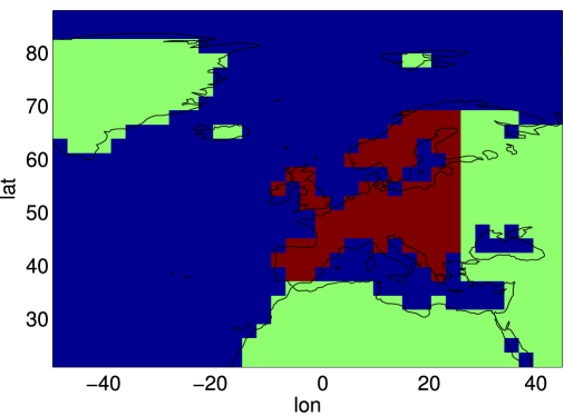
Figure 1: European domain $\Omega$ over which the surface temperature is averaged (in red). Note that here we show a zoom over a region, but the model Plasim simulate the dynamics over the whole globe.

We consider a 1000 year long simulation. We take as target observable the European surface temperature $T_{\Omega}(X(t))$, computed as the average of the local surface temperature $T_{s}(\phi,\lambda,t)$ (where $\phi$ is the latitude and $\lambda$ the longitude), over the domain $\Omega$ shown in figure (1), given by the land area included between 36 °N and 70 °N, and -11 °W and 25 °E. Since the spatial average depends only on time, we explicit in $T_{\Omega}(X(t))$ only the dependence on time of the state of the system, consistently with the notation in the previous section (while in general the state of the system depends on both space and time when we consider an extended system like a climate model).

a)
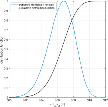
b)

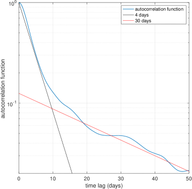
Figure 2: a) Probability distribution function (blue) and cumulative distribution function (black) of the 6 hourly values of the average European surface temperature $T_{\Omega}(X(t))$. Fro graphical reasons the probability distribution function has been normalized so that its maximum has value 1. b) Autocorrelation function of $T_{\Omega}(X(t))$ (blue). The black and red lines show exponential decays on time scales of 4 and 30 days respectively.

Figure (2a) shows the probability density function (normalized so that its maximum has value 1) and cumulative distribution function of the 6 hourly values of $T_{\Omega}(X(t))$. The spatially averaged temperature has mean $\mu\approx 306.5$ $K$ and standard deviation $\sigma\approx 1.6$ $K$, and is slightly asymmetric, with a longer tail for values below the mean. Overall temperatures are rather high if compared with normal climatological summer values, but differences of this order are expected for a perpetual summer simulation without daily cycle. We analyse the large deviation functions of the the anomaly of the spatially averaged temperature with respect to its mean that is, form now on we analyse the observable

$$A(X(t))=T_{\Omega}(X(t))-\mu$$ (10)

Note that, therefore, the mean of $A(X(t))$ is zero. The large deviation rate function $A(X(t))$ and of $T_{\Omega}(X(t))$ is the same up to a translation of $\mu$.

From the 1000 year long run we compute the large deviation functions of the European surface temperature, using the method described in section 3. First of all we study the time required to reach the large deviation asymptotic behavior, which sets the minimum value for the block size $\tau_{b}$. The minimal requirement is that $\tau_{b}$ is much larger than the autocorrelation time of the observable. Figure (2b) shows the autocorrelation function of $A(X(t))$

$$R(t)=\frac{\mathbb{E}\left[A(X(t))A(X(0))\right]}{\sigma^{2}}.$$ (11)

The autocorrelation function is well approximated by a double exponential, with a first decay on time scale $\tau_{s}\approx$4 days, representative of the synoptic fluctuations, and a longer decay on a time scale of about $\tau_{l}\approx$30 days, probably due to the land surface processes, in particular the dynamics of the soil moisture. The integral autocorrelation time, computed as $\tau_{c}=\int_{0}^{+\infty}R(t)\,\textrm{d}t$, results to be $\tau_{c}\approx$ 7.5 days (see Appendix A for the details on the computation of $\tau_{c}$). In terms of applications to the heat wave statistics, an extreme heat wave case can last 1 to 3 months, corresponding to about 4 to 12 autocorrelation times.

a)
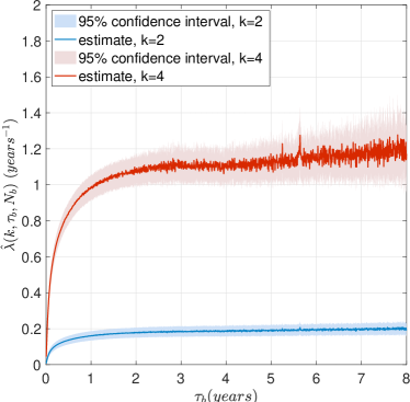
b)
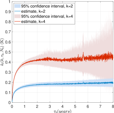
c)

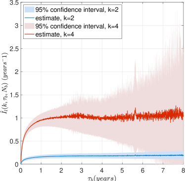
Figure 3: For fixed values of $k$, convergence with the averaging time $\tau_{b}$ of the scaled cumulant generating function $\lambda(k)$ (a), the large deviation estimate of the averaged temperature anomaly $a_{l}=\lambda^{\prime}(k)$ (b), and the large deviation rate function $I(a)$ (c). For each panel the two curves show the results for a value of $k$ inside the region of statistical convergence of both the estimate and its variance ($k=2$, blue), and a value of $k$ inside the region of statistical convergence region of the estimate but not of the variance ($k=4$, red).

The study of the convergence to the large deviation limit shows however that the time necessary to converge is much longer than that. The best value of the block size to have proper convergence is $\tau_{b}=3$ $years$ (see Appendix A). The upper and lower bounds of the convergence region are estimated at $k_{c}^{+}(\tau_{b},N_{b})=5$ $K^{-1}years^{-1}$ and $k_{c}^{-}(\tau_{b},N_{b})=-2.5$ $K^{-1}years^{-1}$. Figures 3a), 3b) and 3c) show the convergence as a function of $\tau_{b}$ of the scaled cumulant generating function, of its derivative, and of the rate function, for two values of $k$: one inside the convergence region of both the estimate and its variance ($k=2$, blue), and one inside the convergence region of the estimate but not of the variance ($k=4$, red).. They correspond to values of the temperature anomaly $a$ of respectively $0.21\>K$ and $0.38\>K$. For example, for $k=2$ the estimated value of $I(a)$ is $0.18\>years^{-1}$, and in order to reach an estimate of $I(a)$ within a relative error of 10% of this value we need $\tau_{b}>1.1\>years$. The analysis of the convergence thus shows that, at the very least, the averaging time should be larger than 1 year to consider to be even approximately in the large deviation asymptotics. Computing a rate function limiting the averaging time to to 40 days and 90 days gives estimates that are about 50% and 65% of the asymptotic result respectively.

The block averaging approach is based on the idea that, whenever the processes is sufficiently mixing, one may consider the time average as an analogous of the sum of $N$ independent variables, $N$ being of the order of $\tau_{b}/\tau_{c}$. As a rule of thumb the convergence towards the large deviation rate function would be expected to be achieved when $N$ is of the order of a few tens. In a case like this, however, we can see that this reasoning is simplistic. The convergence here is extremely slow: the minimal $\tau_{b}$ is much larger than a few times $10\tau_{c}$. The probable reason for this slow convergence is the slowly decreasing long tail of the correlation function of the observable. Indeed, the convergence of the large deviation limit is obtained after about a few years, which is a few times $10\tau_{l}$.

This indicates that the dynamical processes leading to the long decay time $\tau_{l}=30\,\text{days}$ are connected to the dynamics of the extreme fluctuations of the time averaged temperature, which correspond phenomenologically to persistent heat waves. The shorter time scale $\tau_{s}\approx$4 days is compatible with the classical time scale of synoptic variability at midlatitudes, essentially the life cycle of cyclones and anticyclones. The longer time scale $\tau_{l}\approx$30 days is probably due to the low frequency variability of the atmospheric dynamics and to the atmosphere-surface interactions, in particular through the soil moisture dynamics. The soil moisture memory is indeed considered to be a key factor in some of the most extreme heat waves observed in Europe, like the one of 2003 [11, 23, 29].

From our analysis it appears that the large deviation limit per se can not be used to characterize heat waves: due to the presence of the seasonal cycle in the real world, heat waves are of interest up to time period of a season, about 90 days, that as we have seen is far from the time scales for which the large deviation rate function gives meaningful informations. In a recent paper, [13] performed a large deviation analysis of surface temperatures using the model Puma, which consists in the dynamical core of Plasim, obtaining faster convergence rates than what we observe. Puma is essentially Plasim without physical parameterizations, which are substituted by Newtonian cooling. As a consequence the dynamics in Puma does not include the range of processes which determine the surface fluxes of sensible and latent heat, and that lead to memory effects on time scales longer than the synoptic scale. The faster convergence rates is very probably due to this aspect. In more realistic setups, from our analysis it seems unlikely that the statistics of the surface temperature averaged at regional scale could converge to the large deviation limit on time scales shorter that a few years, which makes it not directly relevant for applications.

(a)
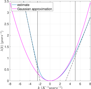
(b)
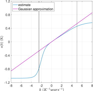
(c)

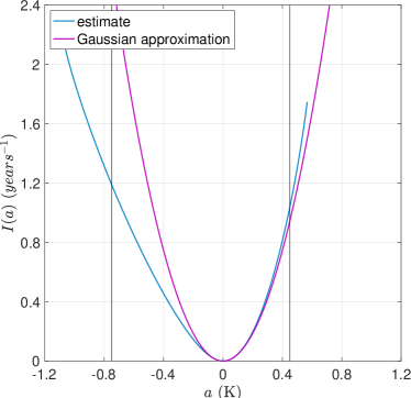
Figure 4: For the time averaged European surface temperature, estimates of $\lambda(k)$ the scaled cumulant generating function (panel a)), $a_{l}=\lambda^{\prime}(k)$ the large deviation estimate of the averaged temperature anomaly (panel b), and $I(a)$ the large deviation rate (c) versus $k$ or $a$ (blue). For each cases, the magenta curves represent the Gaussian approximation.

Figures 4a), 4b) and 4c) show the best estimates from the 1000 year long run of the scaled cumulant generating function , its derivative, and the rate function, with $\tau_{b}$=3 years and $N_{b}=$333. The vertical black lines indicate the boundaries of the convergence region. The dashed black lines show the artificial asymptotic linear behavior of the estimate of the scaled cumulant generating function beyond the convergence region. We see that the large deviation functions are markedly asymmetric. The rate function is steeper for positive anomalies than for negative anomalies, and accordingly the scaled cumulant generating function is larger for positive values than for negative ones. From the definition (2), this means that large persistent temperature anomalies are much more rare than cold anomalies with the same magnitude and duration. This can be quantified at the level of the large deviation rate function. From Figure 4c), one can see that the large deviation rate function value is about the same for a $0.4\,\text{K}$ warm anomaly and for a $-0.7\,\text{K}$ cold anomaly. This means that the probability of $0.4\,\text{K}$ heat wave that lasts a duration $T$, decreases exponential with $T$ at a rate of about $1\,\text{y}^{-1}$ ($I(0.4)\simeq 1\text{y}^{-1}$). The probability of a $-0.7\,\text{K}$ cold spell of duration $T$ decreases at about the same rate ($I(-0.7)\simeq 1\text{y}^{-1}$). However the probability of a $-0.4\,\text{K}$ cold spell of duration $T$ decreases about $2.5$ times slower ($I(-0.4)\simeq 0.4\text{y}^{-1}$).

Note that [13] obtained very symmetric large deviation functions of surface temperature from simulations with the dynamical core of the same model, and noted that the symmetry was likely unrealistic and caused by the lack of a proper representation of moist processes in the model. The fact that in a version of the model that properly takes into account water phase transitions in the atmosphere the rate function is rather asymmetric confirms their observation.

The black vertical lines in figures 4a), 4b) and 4c) show the convergence regions. The temperature anomalies that can be properly sampled with $1\,000$ years of data belong to the range $(-0.8\,\text{\textdegree}\text{K},0.4\,\text{\textdegree}\text{K})$. As one might expect, the corresponding values of the probabilities at the two boundaries of this range are about the same ($I(-0.8)\simeq I(0.4)$). Accordingly the confidence intervals are larger for negative anomalies which are less rare. How does this range compare with the Gaussian range? As can be seen in figures 4, for positive anomalies the estimate in the convergence region is still very close to the Gaussian approximation. For negative anomalies the tail is markedly less Gaussian. This illustrate that long lasting cold spell with a return time of about $1\,000$ years can not be studied with a Gaussian model. In the case of positive anomalies, even 1000 years of data are not enough to observe the non Gaussian tails of the large deviation rate function. In order to explore the far tails of the large deviation functions, one may use rare event algorithms.

4 Estimate of large deviation functions with rare event algorithms

4.1 A large deviation rare event algorithm

Rare event simulation techniques are numerical tools specifically dedicated to the computation of rare events in numerical models at a much smaller computational effort than direct sampling. Such tools have a long history [19] and have attracted a growing interest in the last two decades [28, 4, 15, 6]. The goal of these methods is to make rare events effectively less rare, thereby improving the efficiency of the statistical estimators.

The method we describe in this paper is a genealogical algorithm originally proposed by [7], and subsequently adapted to compute large deviation functions of time averaged observables in numerical models [16, 21]. In [26], we have used this method to study European heat waves, focusing on seasonal time scales. As we discussed in the previous section, such times scales are out of the large deviation asymptotics. Here we show instead how the algorithm can be extremely useful to compute large deviation functions of climate observables, overcoming the limitations of direct estimates. In the following we refer to this algorithm as large deviation algorithm or Giardina-Kurchan-Lecomte-Tailleur (GKLT) algorithm when used to compute large deviation functions, and as the Del Moral-Garnier algorithm when used to simulate rare events outside of the large deviation asymptotics.

We give a general description of the large deviation algorithm; more details are discussed in [26] or in the original papers [16, 21]. We perform simulations of an ensemble of $N$ trajectories $\left\{X_{n}(t)\right\}$ (with $n=1,2,...,N$) starting from different initial conditions. The total integration time of the trajectories is denoted $T_{a}$. We consider an observable $A(X(t))$ of which we want to compute the large deviations. We define a resampling time $\tau$, and during the evolution of the system we perform at times $t_{i}=i\tau$ (with $i=1,2,...,T_{a}/\tau$) a resampling procedure based on the past values of the observable on the trajectories. At time $t_{i}$ we assign to each trajectory $n$ a weight $W_{n}^{i}$ defined as

$$W_{n}^{i}=\frac{e^{k^{*}\intop_{t_{i-1}}^{t_{i}}A(X_{n}(t))\,\text{d}t}}{R_{i}}\,\,\,\mbox{with}\,\,\,R_{i}=\frac{1}{N}\sum_{n=1}^{N}e^{k^{*}\int_{t_{i-1}}^{t_{i}}A(X(t))\,\text{d}t},$$ (12)

where $k^{*}$ is a tuning parameter of the algorithm, whose role is described in the following. For each trajectory $n$, a random number of copies of the trajectory are generated at time $t_{i}$. The expectation value of the number of copies generated by a trajectory $n$is proportional to its weight $W_{n}^{i}$. Trajectories featuring large values of the time average of the observable will thus produce many copies of themselves, while trajectories featuring small values of the observable will not produce any copies and will effectively be killed. For practical reasons it is convenient to generate the copies in such a way to fix the total number of trajectories to be always exactly $N$ after each resampling, as described in [26]. The value of the parameter $k^{*}$ defines how stringent is the selection. For large values of $k^{*}$ only the trajectories with the very largest values of the observable will be allowed to generate copies of themselves. If the system is deterministic, like in the case of climate models, a small random perturbation is added just after the cloning to each trajectory, so that copies of the same trajectory will evolve differently. See [26] for more details.

Once the final time $T_{a}$ is reached and the simulation is over, an effective ensemble is reconstructed by removing all the pieces of trajectories that did not survive until time $T_{a}$. We indicate with $\mathbb{P}_{0}\left(\left\{X(t)\right\}_{0\leq t\leq T_{a}}\right)$ the probability of observing a certain trajectory between time 0 and $T_{a}$ as normally generated by the dynamics of the model, and with $\mathbb{P}_{k^{*}}\left(\left\{X(t)\right\}_{0\leq t\leq T_{a}}\right)$ the probability of observing that same trajectory in the effective ensemble. One can show that

$$\mathbb{P}_{k^{*}}\left(\left\{X(t)\right\}_{0\leq t\leq T_{a}}\right)\underset{N\rightarrow\infty}{\sim}\frac{e^{k^{*}\int_{0}^{T_{a}}A(X(t))dt}}{\mathbb{E}\left[e^{k^{*}\int_{0}^{T_{a}}A(X(t))dt}\right]}\mathbb{\mathbb{P}}_{0}\left(\left\{X(t)\right\}_{0\leq t\leq T_{a}}\right),$$ (13)

where $\underset{N\rightarrow\infty}{\sim}$ means that this is true asymptotically for large $N$ with typical error of order $1/\sqrt{N}$ when evaluating averages over observables. For large positive values of $k^{*}$, the path measure $\mathbb{P}_{k^{*}}$ is thus tilted with respect to $\mathbb{P}_{0}$ such that large values of $a=\frac{1}{T}\int_{0}^{T}A(X_{n}(t))\,\mbox{d}t$ will be favored. In order obtain (13), we have used the mean field approximation

$$R_{i}=\frac{1}{N}\sum_{n=1}^{N}e^{k^{*}\int_{t_{i-1}}^{t_{i}}A(X_{n}(t))dt}\underset{N\rightarrow\infty}{\sim}\mathbb{E}\left[e^{k^{*}\int_{t_{i-1}}^{t_{i}}A(X_{n}(t))dt}\right].$$ (14)

The validity of this approximation and the fact that typical relative errors are of order $1/\sqrt{N}$ have been proved to hold asymptotically for large $N$ by [6], for a family of genealogical algorithms which includes the one adopted here.

The algorithm thus samples very efficiently the tails of the probability distribution $\rho(a,T)$. Equation (13) can be used to compute statistics according to $\mathbb{P}_{0}$ (the original statistics of the system, what we are interested in) from an ensemble of trajectories distributed according to $\mathbb{P}_{k^{*}}$ (obtained with a simulation with the algorithm). An estimator of the expectation value of any quantity $O\left(\left\{X(t)\right\}_{0\leq t\leq T_{a}}\right)$ based on (13) is

$$\mathbb{E}\left[O\left(\left\{X(t)\right\}_{0\leq t\leq T_{a}}\right)\right]\underset{N\rightarrow\infty}{\sim}\frac{1}{N}\sum_{n=1}^{N}\left(e^{-k^{*}\int_{0}^{T_{a}}A(X_{n}(t))\,\text{d}t}\prod_{i=1}^{T_{a}/\tau}R_{i}\right)O\left(\left\{X_{n}(t)\right\}_{0\leq t\leq T_{a}}\right),$$ (15)

where the $X_{n}$ are the $N$ backward reconstructed trajectories present in the effective ensemble. Note that in (15) there is no assumption of $T_{a}$ being large. Since in the tilted ensemble large values of $a=\frac{1}{T}\int_{0}^{T}f(x(t))\,\mbox{d}t$ will be more common, the estimation of the tails of $\rho(a,T)$ will have smaller statistical errors. Tuning $k^{*}$ will allow us to study different ranges of extreme values in the tails of $\rho(a,T)$.

In the limit of very large $T_{a}$, the algorithm provides a direct way to compute very efficiently the scaled cumulant generating function. Using (14) one obtains that the scaled cumulant generating function at $k=k^{*}$ can be computed as

$$\hat{\lambda}(k^{*})=\lim_{T_{a}\rightarrow\infty}\frac{1}{T_{a}}\sum_{i=1}^{T_{a}/\tau}\log\left[R_{i}\right],$$ (16)

with a relative error of order $1/\sqrt{N}$. This is the main output of the large deviation algorithm in its GKLT formulation [16, 21]. From the scaled cumulant generating function one can then compute the rate function as described in the previous section.

In typical applications of the large deviation algorithm [15], the systems under consideration were sufficiently inexpensive to run that it was possible to perform several experiments with different values of $k^{*}$ and compute the scaled cumulant generating function pointwise. With a climate model this is computationally unfeasible. However, equation (13) can be used to compute a very precise estimate of the scaled cumulant generating function in a neighborhood of $k^{*}$. Using (15) an estimator of $\lambda(k)$ is

$$\hat{\lambda}(k)=\hat{\lambda}(k^{*})+\lim_{T_{a}\rightarrow\infty}\frac{1}{T_{a}}\log\left[\frac{1}{N}\sum_{n=1}^{N}e^{(k-k^{*})\int_{0}^{T_{a}}A(X_{n}(t))dt}\right].$$ (17)

Equation (17) gives a very good estimate of the scaled cumulant generating function in a neighborhood of $k^{*}$. This can be seen noting that the typical value of the observable $\frac{1}{T_{a}}\intop_{0}^{T_{a}}A(X(t))dt$ observed in the algorithm statistics in the limit of large $T_{a}$ is, using equation (13),

$$\mathbb{E}_{k^{*}}\left[\lim_{T_{a}\rightarrow+\infty}\frac{1}{T_{a}}\intop_{0}^{T_{a}}A(X(t))\,\mbox{d}t\right]=\lim_{T_{a}\rightarrow+\infty}\mathbb{E}\left[\left(\frac{1}{T_{a}}\intop_{0}^{T_{a}}A(X(t))\,\text{d}t\right)\frac{e^{k^{*}\int_{0}^{T_{a}}A(X(t))\,\text{d}t}}{\mathbb{E}\left[e^{k^{*}\int_{0}^{T_{a}}A(X(t))\,\text{d}t}\right]}\right]=\lambda^{{}^{\prime}}(k^{*}).$$ (18)

Since in the large deviation regime the average and the most probable value coincide as a first approximation, this means that the time average of the observable in the effective ensemble will fluctuate around a typical value given by the derivative of the scaled cumulant generating function evaluated in $k^{*}$. This is exactly the range of fluctuations that are needed in order to compute correctly the large deviation function in a neighborhood of $k^{*}$ [27]. Effectively tilting the trajectory probability density shifts the center of the convergence region of the estimator around $k=k^{*}$. It is therefore possible to perform a few experiments with different values of $k^{*}$, compute the estimate of $\lambda(k)$ for the neighborhoods of the values of $k^{*},$ and then join the estimates to reconstruct $\lambda(k)$ piecewise. This allows to explore the tails of the scaled cumulant generating function (hence of the rate function) with a huge gain in terms of computational cost with respect to direct estimation methods.

4.2 Analysis of large deviations of Europe surface temperature in a climate model with the large deviation algorithm

We demonstrate here the performances of the large deviation algorithm applied to the climate model Plasim to compute the large deviation functions of the European surface temperature. We use the direct estimate obtained with the 1000 years long control run as a benchmark and show that with the algorithm it is possible to compute the same values of the large deviation functions with a smaller computational cost.

The experiments are carried out for different values of $k^{*}$ with $N=128$ trajectories, each run for a total time $T_{a}=$800 days. Each experiment has thus a total computational cost of about 284 years. The initial conditions of the trajectories are taken from the control run, spaced by a few years from each other to ensure statistical independence. The first 80 days of simulations are considered as a transient to reach statistical equilibrium, and the statistical analysis is performed on the last 720 days. The resampling time is set at 8 days, as in [26]. The choice of the resampling time is determined by how trajectories starting from the same initial condition separate in time after the addition of a small random perturbation. Heuristically it is expected that a good choice should be $\tau$ to be of the order of $\tau_{c}$. If the resampling time is much smaller than the autocorrelation time of the process, the trajectories do not have time to separate enough and useless resampling will increase the variance. If on the contrary the resampling time is much larger than the autocorrelation time, the trajectories will fall back to the typical states, and the importance sampling efficiency will be lost. Tests with simpler systems [22] have shown that the precise value of $\tau$ does not affect the results, as long as it is of the order of the autocorrelation time. The trajectories are perturbed after cloning by adding a small random field to the surface pressure, as described in [26].

(a)
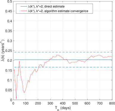
(b)

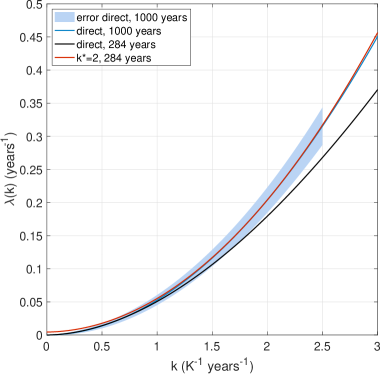
Figure 5: (a) Estimate of $\lambda(k^{*})$ with $k^{*}=2$. The blue solid line indicates the reference value obtained from the control run, with the blue dashed lines indicating the 95% confidence interval. The red line shows the convergence of the estimate obtained with the algorithm as a function of the length of the simulation $T_{p}$. From simulations of 300 days or longer the estimate of $\lambda(k^{*})$ oscillates stably well inside the 95% confidence interval of the direct estimate. (b) Direct estimate of the scaled cumulant generating function from the 1000 years long control run (blue), direct estimate from the control run using only 284 years (black) and estimate with the algorithm with $k^{*}=2$ (red).

We first consider $k^{*}=2$, a value for which the direct estimate of the large deviation rate function with the 1000 years control run converges. Figure 5 shows the convergence of the estimate obtained with the algorithm as a function of the length of the simulation, that is the quantity

$$\hat{\lambda}(k^{*})=\frac{1}{T_{p}}\sum_{i=1}^{T_{p}/\tau}\log\left[R_{i}\right],$$ (19)

with the partial simulation length going from $T_{p}=0$ to $T_{p}=T_{a}=800$ days. From simulations of 300 days or longer the estimate of $\lambda(k^{*})$ oscillates stably well inside the 95% confidence interval of the direct estimate. Note that $T_{p}=300$ days corresponds to a total computational cost of about 107 years. The convergence speed depends on the value of $k^{*}$, hence the choice of considering in general a length of $T_{p}=T_{a}=800$ days, to stay on the safe side. The estimate of $\lambda(k^{*})$ using the algorithm is a sum of $T_{a}/\tau$ values, each for each resampling. We can associate to the estimate an error as the standard deviation associated to such sum, divided by the square root of $T_{a}/\tau$. In this case we have that for $k^{*}=2$ the rare event algorithm estimate gives $\lambda(k^{*})=0.218\pm 0.025$ against a direct estimate of $\lambda(k^{*})=0.204\pm 0.038$.

The data from the large deviation algorithm can also be used also to estimate $\lambda(k)$ in a neighborhood of $k^{*}$. Figure 16b shows the estimate of $\lambda(k)$ for $0<k<3$ obtained with the experiment with $k^{*}=2$ , using equation (17), compared with the direct estimate obtained from a 1000 years of control run and with a direct estimate obtained using only 284 years of the control run. We can see that the estimate of the large deviation algorithm perfectly coincides with the direct estimate from the long run in its convergence region. By contrast the direct estimate for short control run performs poorly for $k>1$, due to the lack of statistics. In particular, for $k>1.75$ the estimate is outside of the confidence interval of the direct estimate from the long control run, so that the short control run estimate is clearly wrong for those values of $k$. As already said, the large deviation algorithm essentially shifts the center of the convergence region from $k=0$ to $k=k^{*}$ . Consequently, the best agreement with the benchmark is obtained for $k=2$, while the agreement is slightly worse close to $k=0$. We can conclude that indeed the large deviation algorithm outperforms the estimation of the scale cumulant generating functions in range of $k$ centered around the value used in the algorithm.

One can use the algorithm to extend the estimates to values of $k$ that are outside the convergence region of the long control run, for which we would need an extremely long simulation in order to use the direct sampling method. The idea is to perform a series of $N_{k}$ experiments with different values of $k^{*}=k_{i}^{*}$, with $i=1,2,...,N_{k}$, each providing a local estimate $\hat{\lambda}_{i}(k,\tau_{b},N_{b})$ around $k_{i}^{*}$. We then reconstruct the scaled cumulant generating function, for instance by piecewise linear approximations $\hat{\lambda}(k)=\alpha_{i}\hat{\lambda}_{i}(k)+(1-\alpha_{i})\hat{\lambda}_{i+1}(k),\,\,\,\mbox{with}\,\,\,k_{i}^{*}\leq k<k_{i+1}^{*}$ where $\alpha_{i}=(k_{i+1}^{*}-k)/(k_{i+1}^{*}-k_{i}^{*}).$ In order to make a proper analysis we have to add an uncertainty to the estimates. However, in the case of the large deviation algorithm we have no rigorous results on the range of convergence of the estimator and of its variance. Empirical analysis shows that the estimates of the scale cumulant generating function obtained with the large deviation algorithm suffers from the same linearization problem as the direct estimate, only with the center of the convergence region shifted around $k=k^{*}$. Therefore, we can estimate the error of the scale cumulant generating function and its range of convergence by simply mimicking what we did in the case of the direct method.

(a)
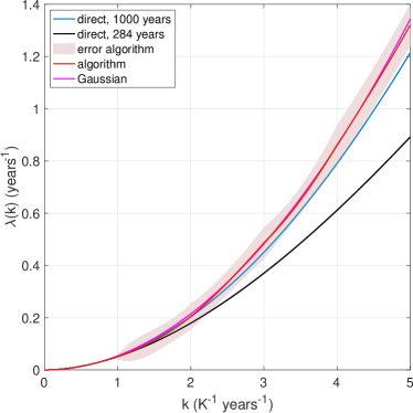
(b)

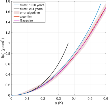
Figure 6: (a) Direct estimate of the scaled cumulant generating function from the 1000 years control run (blue), direct estimate from the 284 years control run (black) and estimate obtained combining the results obtained with the algorithm with $k^{*}=2,3,4$ (red). (b) The same for the rate function.

Figure 6 shows the scaled cumulant generating function reconstructed in this way using three experiments with $k^{*}=2,3,4$. For $0\leq k<1$ we have used only the 284 years direct estimate, for $1\leq k<2$ we have used the 284 years direct estimate and the $k^{*}=2$ estimate, and for $k\geq 2$ we have used the method described above. We note that the 284 year direct estimate is clearly wrong for large values of $k$. Moreover, for $k>3.5$, the 1000 years control run estimate is outside the error bar of the large deviation algorithm estimate, which is the most reliable in this range. This is consistent with last section results that concluded that the 1000 years control run estimate is unreliable for $k>2.5$. We would have needed much more than 1000 years of data in order to have a reliable direct estimate for those values of $k$.

Somehow surprisingly, looking at figure 6, we learn that the large deviation function for warm anomalies is extremely Gaussian. Relying only on direct estimates without performing a proper convergence analysis, we may have led us to the wrong conclusion that 1000 years of data would have been sufficient to go beyond the Gaussian regime. Instead, the large deviation functions are Gaussian well beyond the convergence region of the direct estimate even for such a long run. If one is interested in computing the non Gaussian part of the tail the use of rare event sampling techniques seem thus of vital importance. A piecewise reconstruction of the large deviation functions with the algorithm can seem computationally expensive, as one has to perform several experiments for different values of $k^{*}$. However, in this case the computational cost grows linearly with the size of the range of $k$ one wants to explore, while in the case of the direct estimate it grows exponentially, making a proper analysis impossible.

5 Using the large deviation algorithm for extreme heat waves

As we have discussed, the time scales required to reach the large deviation asymptotics are too long for the large deviation rate functions to be relevant to discuss seasonal heat waves or cold spells. However, the rare event algorithm itself [7] does not need $T_{a}$ to be in the large deviation asymptotics. In [26] we have exploited this property to show how the algorithm could be used to sample extremely rare heat waves with return times up to millions of years, with computational costs two to three orders of magnitude smaller. Here we recall the main results of [26], connecting them more explicitly with the previous sections.

We are interested in computing the tail of the distribution of the European surface temperature time averaged over a time $T$ of interest for applications. The strongest heat waves are characterized by persistence at scales from sub-seasonal to seasonal (between a few weeks and 3 months). This value of $T$ is more than one order of magnitude smaller than the values we have considered in the previous section. Consequently, the value of the algorithm parameter $k^{*}$ must be chosen carefully. The value of the parameter $k^{*}$ determines the most probable value of the fluctuations observed in a simulation with the algorithm, independently of the value of $T$. When we lower $T$ to study time scales more realistic for heat waves, the width of $\rho(a,T)$ increases substantially. This means that the values of the fluctuations $a$that one obtains with the values of $k^{*}$ that used in the previous section to study the large deviation limit will not correspond to very rare events for smaller values of $T$. Therefore we need to use values of the biasing parameter $k^{*}$ much larger than those used in the large deviation limit, to reach fluctuations that are rare for the new values of $T$.

The choice of the range of values of $k^{*}$ to be used depends on the value of the averaging time $T$ and on the range on temperature anomalies $a$ that one wants to analyze. In the large deviation limit, the relation $\mathbb{E}_{k^{*}}[a]=\lambda^{\prime}(k^{*})$ can be used to choose the value of $k^{*}.$ For smaller $T$ the relation does not hold anymore. However, one can still think to use it to get a rough estimate at least of the order of magnitude of the value of $k^{*}$ necessary to target a certain range of fluctuations. Since the value of $k^{*}$ to be used is very large, a direct estimate of $\lambda(k^{*})$ and thus $\lambda^{\prime}(k^{*})$ is not be available, for the reasons discussed in the previous sections. One could use then the Gaussian approximation of the scaled cumulant generating function to have at least the order of magnitude of $k^{*}$ necessary to observe fluctuations of order $a$, obtaining $k^{*}\approx a/\left(2\tau_{c}\sigma^{2}\right)$. This is a very crude approximation, but it is still better than a blind guess.

(a)
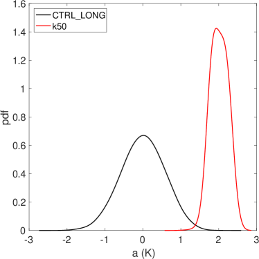
(b)

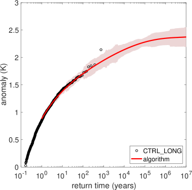
Figure 7: (a) Probability distribution function of the 90 days average European surface temperature, from the control run (black) and the $k^{*}=50$ experiment (red). (b) Return time of the 90 days average European surface temperature, from the control run (black) and the experiments with $k^{*}=10,20,40,50$ experiments (red).

As a test case, we study $T=90$ days. The domain of $k$ over which the scaled cumulant generating function is known, from the long control run, with an acceptable degree of accuracy is too narrow to include values of the derivative of the scaled cumulant generating function above $\sim 1\>K$. The black curve of figure 7a shows the probability distribution of the 90 days averaged European surface temperature estimated from the 1000 years long control run. We can see that a threshold on 1 K does not actually select extremely rare events, confirming the discussion above. In the following we study heat waves for which the time averaged Europe surface temperature during $T=90$ is larger than $a=2\,\text{K}$, that are extremely rare. Using the Gaussian approximation of the scaled cumulant generating function, we infer that the value of $k^{*}$ for which fluctuations of order $a=2\>K$ are typical is $k\approx 19$. Since this is an order of magnitude argument, we consider for our experiments four different values, $k^{*}=10,20,40,50$.

The resampling time $\tau$ is kept at 8 days, while the length of the simulations and the number of trajectories are changed with respect to the case of the large deviation limit. While in the case of the computation of the large deviation function it was crucial to wait for the system to reach statistical equilibrium, and thus $T_{a}$ had to be very large, in this case it is sufficient to take $T_{a}$ at least larger than 90 days to resolve both the transient leading to the extreme heat wave and the heat wave itself. Since the value of $k^{*}$ is be much larger than in the large deviation case, it is necessary to have a larger number of trajectories, in order to avoid ending up with an effective ensemble populated by the clones of just one trajectory. We set $T_{a}=128$ days and $N=512$ trajectories. Each experiment has thus a computational cost of about 182 years.

Figure 7a) shows the probability distribution function of the 90 day average of the European surface temperature for the experiment with $k^{*}=50$ compared with the probability distribution function of the control run. We can see that indeed the distribution of the anomalies of the 90 days averaged temperature is heavily shifted towards positive values. For a $2\,\text{K}$ threshold, in the $k^{*}=50$ experiment the system is in heat wave conditions in about 50% of the trajectories. Thanks to importance sampling, we can hugely improve the estimate of the statistics of the events belonging to the tail of the original distribution.

The return time of extreme events is an important characterization of extremes. Figure 7b) shows the return time of the anomalies of the 90 days temperature, estimated from the 1000 years long control run (black). With direct sampling clearly we can not estimate correctly events with return time larger than a few centuries. Thanks to the rare event algorithm, we can extend the estimate of the return time curve to much rarer events. The return time can be computed from the output of the rare event algorithm as described in details in [26] and [22]. The red line in figure 7b) has been obtained by computing return time functions from the experiments with the algorithm (the case $k^{*}=20$ and $k^{*}=40$ repeated twice with different sets of initial conditions to improve the statistics) and averaging the results in the areas of overlap. Using several experiments with different values of $k^{*}$ and different sets of initial conditions helps to improve the statistics and to obtain a better estimate. The total computational cost of the experiments is of about 1090 years, basically the same of the control run. We can see that the return time curve obtained with the large deviation algorithm overlaps with the upper part of the curve given by the control run (confirming the correctness of the procedure), but extends to much larger values of the return time. With the algorithm we can compute return times up to $10^{6}-10^{7}$ years with a total computational cost of the order of $10^{3}$ years. There is thus a gain of more than three orders of magnitude in the sampling efficiency.

This result has two implications. First, in this way it is possible to observe ultra rare events that could never be observed in a direct numerical simulation, unless one employs an unrealistic amount of computational resources. Second, and possibly more importantly, the quality of the statistics of rare events in general is greatly improved. For example, in 1000 years in the control run there is only one event with temperature in excess of 2 K during the 90 days period. With the rare event algorithm instead, we have access to several hundreds of them even considering only one of the experiments, at a fraction of the computational cost. This improvement of the statistics allows to perform studies of extreme events that are out of reach with standard direct sampling.

We can for example compute composite maps of the surface temperature anomalies and of the 500 hPa geopotential height anomalies, conditional on the occurrence of an heat wave. This kind of composite statistics is sometimes used in the study of climatic extremes, in order to detect the typical dynamical patterns connected to the extremes of interest. For example, [29] provided a classification of European heat waves by performing a cluster analysis of composites of heat wave events, although the condition of occurrence of an heat wave in their case was defined in a more complex way than in this study. How can this type of analysis be performed with data obtained with the large deviation algorithm? Let us write either the surface temperature or the 500 hPa geopotential height anomaly field as $O\left(X(t)\right)$, and the condition of occurrence of the heat wave as $\frac{1}{T}\int_{0}^{T}A(X(t))dt>a$, with $T$=90 days and $a$= 2 K. The conditional expectation value can be computed as

$$\mathbb{E}\left[O\left(X(t)\right)\left|\,\frac{1}{T}\intop_{0}^{T}A\left(X(t)\right)dt>a\right.\right]=\frac{\mathbb{E}\left[O\left(X(t)\right)\Theta\left(\frac{1}{T}\int_{0}^{T}A\left(X(t)\right)dt-a\right)\right]}{\mathbb{E}\left[\Theta\left(\frac{1}{T}\int_{0}^{T}A\left(X(t)\right)dt-a\right)\right]},$$ (20)

where $\Theta(\cdot)$ is the Heaviside function. Empirical estimators of conditional expectation values can be easily extended to the case of the tilted trajectory probability by using (15) at numerator and denominator of (20).

(a)
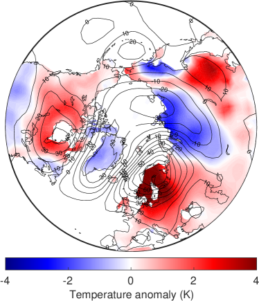
(b)

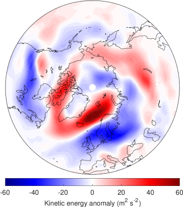
Figure 8: (a) Surface temperature anomaly (colors) and 500 hPa geopotential height anomaly (contours) for the k50 experiment, conditional on the occurrence of heat wave conditions. (b) Horizontal kinetic energy anomaly at 500 hPa for the k50 experiment, conditional on the occurrence of heat wave conditions.

Figure 8a) shows the composite average of surface temperature and 500 hPa geopotential height anomalies over the Northern hemisphere above 35° latitude, conditional on the occurrence of an European heat wave, estimated from the large deviation algorithm with $k^{*}=50$. The heat wave pattern shows an extended warming over Europe. The warm anomaly is larger over Scandinavia than over the rest of Europe. The 500 hPa geopotential height field show a strong anticyclonic anomaly right above the area experiencing the maximum warming, as expected in heat wave conditions. Overall the pattern over Europe is qualitatively very similar to the Scandinavian heat wave cluster detected by [29]. However, it appears connected to a teleconnection pattern spanning the entire Northern Hemisphere, with an apparent wavenumber 3 structure. The 500 hPa geopotential height anomalies in the North Atlantic/European area are consistent with a southward shift of the jet stream over the North Atlantic and a northward shift of the jet stream over continental Europe, as shown in 8 b), where we plot the composite of the kinetic energy related to the horizontal motion, as anomalies with respect to the control run.

Note that usual teleconnection patterns are computed typically through empirical orthogonal functions analysis or similar techniques, and thus describe pattern for typical fluctuations of the atmosphere. Extreme event conditional statistics are instead related to very rare states of the flow characterizing the extreme events. With $T$=90 days and $a$=2 K, the events that we have selected have return times larger than 1000 years. Thanks to this method it is thus possible to compute these maps with a sufficient degree of precision to be able to robustly speak of teleconnection patterns for extreme events.

6 Conclusions

In this paper we have discussed techniques to compute large deviation functions of climatic observables. Direct estimation of large deviation functions in a complex chaotic system is a delicate procedure that needs care in properly checking the convergence of both the large deviation limit and of the statistical estimators [27]. A simplistic analysis relying on visual arguments for the collapse of the scaled functions on some seemingly well behaved function can lead to wrong estimates, as the functions will indeed converge, but to wrong values. In particular, wrong estimates may lead to think that the available data were enough to go beyond the Gaussian regime, while as we have seen there may be cases in which a more refined analysis shows that non Gaussian behaviors can appear as an artifact of not having properly studied the convergence.

The rare event algorithm described in this paper [7, 16, 21] can greatly help to compute large deviation rate functions for large values of the anomalies that cannot be accessed with a direct approach. This method was never used for systems of the complexity of a numerical climate model, until in [26] we have used it to study European heat waves. In this paper we have used it for the explicit task of computing large deviation rate functions, highlighting its connection to large deviation theory. The recipe presented in this paper can be easily replicated for climate studies on different observables and with different climate models.

We have observed that the large deviation limit is not of direct interest for studying real heat waves. From a physical point of view, the problem is that in the model Plasim with physical parameterizations, the autocorrelation function of the European temperature has a slow decaying tail that involves time scales of about $30$ days. The consequence of this slow decorrelation is that the large time asymptotics of the large deviation rate function is not attained before a few years. This makes the use of the large deviation asymptotics irrelevant for this case for time averages of the order of a few months. The large deviation limit could however be of practical relevance for quantities with faster decaying autocorrelation functions, for example precipitation, or for spatial averages of surface temperature over different regions.

Moreover, algorithms initially dedicated to the computation of large deviations are still efficient to compute the probability of extreme heat waves. The results show in this paper and in [26] refer to a perpetual summer setup, with no time dependent external forcing acting on the system. In the applications envisioned by [16] and [21], the algorithm was not meant to be applied in presence of a time dependent forcing on time scales comparable with the duration of the events of interest, while in the original formulation of [7] there are not limitations in this sense. The daily cycle is shorter than the resampling time, so that including it does not present any problem. We are currently testing the performances of the algorithm in presence of seasonal cycle, that will be the subject of future studies. Even in the form presented in this paper however, the large deviation algorithm could be of extreme interest for application to more theoretical studies in which perpetual summer condition are a common setup.

Appendix A Convergence of direct estimate of large deviation functions and statistical errors

The choice of the size of the time block $\tau_{b}$ and the test of the convergence to the large deviation limit requires computing the autocorrelation time of the process, which sets a lower bound to the values of the averaging time that it makes sense to consider. Figure 2b) shows for the first 50 days the autocorrelation function $R(t)$ of the average European surface temperature $T_{s}$ computed from a 1000 years long run. We can see that to a first approximation the function is well described by a double exponential, with a first decay time of about 4 days compatible with the time scale of synoptic variability, followed by a slowly decaying tail that at least in the first part seems to decay exponentially on a time scale of one month. The longer time scales inducing the slow decay of the autocorrelation function could be related to the low frequency variability of the atmospheric dynamics, and/or to time scales relate to the water vapor cycle in the atmosphere and the land surface processes.

The integral autocorrelation time $\tau_{c}$ is defined as the integral from time lag 0 to $+\infty$ of the autocorrelation function $R(t)=\mathbb{E}\left[(A(X(t))-\mu)(A(X(0))-\mu)\right]/\sigma^{2}$. An equivalent expression for $\tau_{c}$ is [3]

$$\tau_{c}=\frac{1}{2\sigma^{2}}\lim_{\tau_{b}\rightarrow+\infty}\frac{1}{\tau_{b}}\int_{0}^{\tau_{b}}\int_{0}^{\tau_{b}}\mathbb{E}\left[\left(A(X(t))-\mu\right)\left(A(X(s))-\mu\right)\right]dtds.$$ (21)

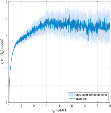
Figure 9: Convergence with $\tau_{b}$ of autocorrelation time.

Equation 21 gives a better estimator of the autocorrelation time than a simple time integration of the autocorrelation function. In practice what we do is to divide the time series in $N_{b}$ blocks of length $\tau_{b}$, and then we compute the integrals in (21) in each block and approximate the expectation value as a sum of the $N_{b}$ blocks. Figure 9 shows the value of the estimate of the autocorrelation time as a function of $\tau_{b}$. The shaded area represents the 95% confidence interval of the estimate computed as two standard deviations of the sample of estimates over the $N_{b}$ blocks. We can see that the estimate converges to a value of about 7.5 days, but that it is necessary to use a very large value of $\tau_{b}$, of at least 3 years, in order to reach convergence.

Once computed the autocorrelation time, the first step of the direct estimate is to compute the generating function

$$\hat{G}(k,\tau_{b},N_{b})=\frac{1}{N_{b}}\sum_{j=1}^{N_{b}}e^{kA_{\tau_{b}}^{j}},\mathrm{with}\;A_{\tau_{b}}^{j}=\frac{1}{\tau_{b}}\intop_{(j-1)\tau_{b}}^{j\tau_{b}}A(X(t))dt$$ (22)

knowing that $\tau_{b}$ will have to be much larger than $\tau_{c}$. When we deal with a discrete time series as the output of a numerical model, where time is discretized in time steps of length $\Delta t$, this means in practice computing

$$\hat{G}(k,\tau_{b},N_{b})=\frac{1}{N_{b}}\sum_{j=0}^{N_{b}-1}e^{k\sum_{n=jp+1}^{jp+p}A(X(n\Delta t))\Delta t},$$ (23)

where $p=\tau_{b}/\Delta t$. Following [3], a more sophisticated way that makes a better use of the available data would be to compute

$$\hat{G}(k,\tau_{b},N_{b})=\frac{1}{2N_{b}}\sum_{j=0}^{2N_{b}-1}e^{k\sum_{n=jp/2+1}^{jp/2+p}A(X(n\Delta t))\Delta t}.$$ (24)

In (24) the sample mean is computed on $2N_{b}$ blocks overlapping by 50%, as suggested by the Welch’s estimator of the power spectrum of a random process [32]. Using (24) instead of (23) does not change the results of the estimate or the convergence region, but gives smaller statistical errors where they can be computed. In the following we keep the simpler notation (22) for ease of presentation.

As discussed in the main text, in a practical application one is constrained by the fixed length $T$ of the time-series, and the choice of $\tau_{b}$ and $N_{b}$ has to be considered carefully. The convergence of the estimators has been studied by [27]. In the case of unbounded variables, obtaining a correct estimate is limited by two problems: 1) the artificial linearization of the tails of the functions due to the finite size of the sample and 2) the non-uniform convergence for different values of $k$.

The linearization effect is an artifact in the estimate of $\hat{G}(k,\tau_{b},N_{b})$ for large values of $k$ which causes the estimate of $\hat{\lambda}(k,\tau_{b},N_{b})$ to become linear in $k$ for any value of $k$ whose module is large enough. This is due to the fact that a sum of exponentials over a finite sample, as the one involved in (22), is dominated for large $k$ by the largest value in the sample, so that $\sum_{j=1}^{N_{b}}e^{kA_{\tau_{b}}^{j}}\approx e^{kA_{\tau_{b}}^{max}}$, with $A_{\tau_{b}}^{max}=\max_{j}\{A_{\tau_{b}}^{j}\}$. Therefore, for a given pair of $\tau_{b}$ and $N_{b}$, for positive $k$ there is an upper critical value $k_{c}^{+}(\tau_{b},N_{b})>0$ for which $\hat{\lambda}(k,\tau_{b},N_{b})\approx kA_{\tau_{b}}^{max}$ for $k>k_{c}^{+}(\tau_{b},N_{b})$. Equivalently for negative $k$ there is a lower critical value $k_{c}^{-}(\tau_{b},N_{b})<0$ for which $\hat{\lambda}(k,\tau_{b},N_{b})\approx kA_{\tau_{b}}^{min}$ for $k<k_{c}^{-}(\tau_{b},N_{b})$. If an observable is bounded, the linear behavior is actually correct. For unbounded variables it is instead an artifact of the finite size of the sample.

Scaling arguments can be provided to estimate $k_{c}^{+}(\tau_{b},N_{b})$ and $k_{c}^{-}(\tau_{b},N_{b})$, as discussed in details in [27]. However, the actual values depend on the underlying probability distribution of the process, and in complex applications they have to be estimated case by case by empirical analysis. A simple way to proceed is to compute the relative contribution of the largest value to the sample mean

$$r(k,\tau_{b},N_{b})=\frac{e^{kA_{\tau_{b}}^{max}}}{\sum_{j=1}^{N_{b}}e^{kA_{\tau_{b}}^{j}}}.$$ (25)

a)
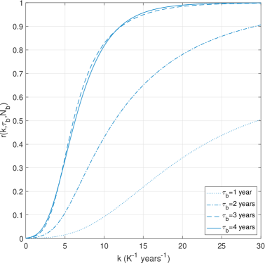
b)

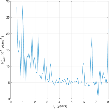
Figure 10: (a) Contribution of the largest value in the sample to the estimate of the generating function as a function of $k$ for different values of $\tau_{b}$. (b) Estimate of upper convergence limit as a function of $\tau_{b}$, taking as threshold a 50% contribution from the largest value in the sample.

By fixing an arbitrary upper threshold for $r(k,\tau_{b},N_{b})$, one finds an estimate for the value of $k_{c}^{+}(\tau_{b},N_{b})$ (and an equivalent procedure gives a value for $k_{c}^{-}(\tau_{b},N_{b})$ ). Figure 10a) shows $r(k,\tau_{b},N_{b})$ as a function of $k$ for different values of $\tau_{b}$ for which there is actual convergence to the large deviation limit. Figure 10b) shows the estimate of $k_{c}^{+}(\tau_{b},N_{b})$ as a function of $\tau_{b}$, obtained taking a threshold of 50% for $r(k,\tau_{b},N_{b})$. We can see that there is a large difference in $k_{c}^{+}(\tau_{b},N_{b})$ if taking a value of $\tau_{b}$ of about 1 year or 3-4 years. However, the estimate for lower values of $\tau_{b}$ is extremely unstable, showing that if proper convergence in time is not reached, also the convergence of the statistical estimator itself is not well behaved. For $\tau_{b}$ larger than 3 years the estimate of $k_{c}^{+}(\tau_{b},N_{b})$ stabilizes around a value of 5 $K^{-1}years^{-1}$. We have therefore taken $\tau_{b}=3$ years and $k_{c}^{+}(\tau_{b},N_{b})=5\>K^{-1}years^{-1}.$ A similar analysis gives $k_{c}^{-}(\tau_{b},N_{b})=-2.5\>K^{-1}years^{-1}$.

Once identified the convergence region of, one can compute statistical errors in half of it, following [27]. The error on the generating function can be naturally estimated as

$$\mathsf{\mathfrak{\textrm{err}}}[\hat{G}(k,\tau_{b},N_{b})]=\sqrt{\mathrm{var}(\hat{G}(k,\tau_{b},N_{b}))/N_{b}},$$ (26)

where $\mathrm{var}(\hat{G}(k,\tau_{b},N_{b}))$ is the empirical variance associated with the sample mean replacing the expectation value. An estimate of the associated error on $\hat{\lambda}(k,\tau_{b},N_{b})$ can be computed by taking a Taylor expansion of the estimator [25, 27]

$$\mathsf{\mathfrak{\textrm{err}}}[\hat{\lambda}(k,\tau_{b},N_{b})]=\frac{\mathsf{\mathfrak{\textrm{err}}}[\hat{G}(k,\tau_{b},N_{b})]}{\hat{G}(k,\tau_{b},N_{b})}.$$ (27)

The statistical error on $\hat{a}(k,\tau_{b},N_{b})$ can be estimated by

$$\mathsf{\mathfrak{\textrm{err}}}[\hat{a}(k,\tau_{b},N_{b})]=\sqrt{\frac{\mathsf{\mathfrak{\textrm{err}}}[\hat{H}(k,\tau_{b},N_{b})]^{2}}{\left(\hat{G}(k,\tau_{b},N_{b})\right)^{2}}+\frac{\left(\hat{H}(k,\tau_{b},N_{b})\right)^{2}\mathsf{\mathfrak{\textrm{err}}}[\hat{G}(k,\tau_{b},N_{b})]^{2}}{\left(\hat{G}(k,\tau_{b},N_{b})\right)^{4}}},$$ (28)

where $\hat{H}(k,\tau_{b},N_{b})=\sum_{j=1}^{N_{b}}A_{\tau_{b}}^{j}e^{kA_{\tau_{b}}^{j}}$ and $\mathsf{\mathfrak{\textrm{err}}}[\hat{H}(k,\tau_{b},N_{b})]$ is computed as $\mathsf{\mathfrak{\textrm{err}}}[\hat{G}(k,\tau_{b},N_{b})]$. This formula is obtained assuming that $\hat{H}(k,\tau_{b},N_{b})$ and $\hat{G}(k,\tau_{b},N_{b})$ are independent [27]. The error on $\hat{I}(\hat{a}(k,\tau_{b},N_{b}),\tau_{b},N_{b})$ can then be estimated as

$$\mathsf{\mathfrak{\textrm{err}}}[\hat{I}(\hat{a}(k,\tau_{b},N_{b}),\tau_{b},N_{b})]=\sqrt{k\mathsf{\mathfrak{{}^{2}\textrm{err}}}[\hat{a}(k,\tau_{b},N_{b})+\mathsf{\mathfrak{\textrm{err}}}[\hat{\lambda}(k,\tau_{b},N_{b})}.$$ (29)

again assuming independence between $\hat{a}(k,\tau_{b},N_{b})$ and $\hat{\lambda}(k,\tau_{b},N_{b})$.

Conflict of interest

The authors declare that they have no conflict of interest.

References

- [1] AghaKouchak, A.: Extremes in a changing climate detection, analysis and uncertainty. Springer, Dordrecht; New York (2012)
- [2] Ailliot, P., Allard, D., Monbet, V., Naveau, P.: Stochastic weather generators: an overview of weather type models. Journal de la Societe Francaise de Statistique 156(1), 101–113 (2015)
- [3] Bouchet, F., Marston, J.B., Tangarife, T.: Fluctuations and large deviations of reynolds stresses in zonal jet dynamics. Physics of Fluids 30(1), 015110 (2018). DOI 10.1063/1.4990509
- [4] Bucklew, J.A.: An introduction to rare event simulation. Springer, New York (2004)
- [5] Coles, S.: An Introduction to Statistical Modeling of Extreme Values. Springer-Verlag, New York (2001)
- [6] Del Moral, P.: Feynman-Kac Formulae Genealogical and Interacting Particle Systems with Applications. Springer New York (2004)
- [7] Del Moral, P., Garnier, J.: Genealogical particle analysis of rare events. The Annals of Applied Probability 15(4), 2496–2534 (2005). DOI 10.1214/105051605000000566
- [8] Dembo, A., Zeitouni, O.: Large Deviations and Applications, in Handbook of stochastic analysis and application. CRC Press (2001)
- [9] Donsker, M.D., Varadhan, S.S.: Asymptotic evaluation of certain markov process expectations for large time, i. Communications on Pure and Applied Mathematics 28(1), 1–47 (1975)
- [10] Ellis, R.S.: Entropy, large deviations, and statistical mechanics. Springer (2007)
- [11] Fischer, E.M., Seneviratne, S.I., Vidale, P.L., Luthi, D., Schaer, C.: Soil moisture-atmosphere interactions during the 2003 european summer heat wave. Journal of Climate 20(20), 5081–5099 (2007). DOI 10.1175/JCLI4288.1
- [12] Fraedrich, K., Jansen, H., Luksch, U., Lunkeit, F.: The Planet Simulator: towards a user friendly model. Meteorol. Z. 14, 299–304 (2005)
- [13] Galfi, V.M., Lucarini, V., Wouters, J.: A large deviation theory-based analysis of heat waves and cold spells in a simplified model of the general circulation of the atmosphere. Journal of Statistical Mechanics: Theory and Experiment 2019(3), 033404 (2019). DOI 10.1088/1742-5468/ab02e8
- [14] Ghil, M., Yiou, P., Hallegatte, S., Malamud, B., Naveau, P., Soloviev, A., Friederichs, P., Keilis-Borok, V., Kondrashov, D., Kossobokov, V., Mestre, O., Nicolis, C., Rust, H., Shebalin, P., Vrac, M., Witt, A., Zaliapin, I.: Extreme events: dynamics, statistics and prediction. Nonlinear Processes in Geophysics 18(3), 295–350 (2011). DOI 10.5194/npg-18-295-2011
- [15] Giardina, C., Kurchan, J., Lecomte, V., Tailleur, J.: Simulating rare events in dynamical processes. Journal of Statistical Physics 145(4), 787–811 (2011). DOI 10.1007/s10955-011-0350-4
- [16] Giardina, C., Kurchan, J., Peliti, L.: Direct evaluation of large-deviation functions. Physical Review Letters 96(12), 120603 (2006). DOI 10.1103/PhysRevLett.96.120603
- [17] IPCC: Managing the risks of extreme events and disasters to advance climate change adaption: special report of the Intergovernmental Panel on Climate Change. Cambridge University Press, New York, NY (2012)
- [18] IPCC: Climate Change 2013: The Physical Science Basis. Contribution of Working Group I to the Fifth Assessment Report of the Intergovernmental Panel on Climate Change. Cambridge University Press, Cambridge, United Kingdom and New York, NY, USA (2013)
- [19] Kahn, H., Harris, T.E.: Estimation of particle transmission by random sampling. National Bureau of Standards applied mathematics series 12, 27–30 (1951)
- [20] Kifer, Y.: Large deviations in dynamical systems and stochastic processes. Transactions of the American Mathematical Society 321(2), 505–524 (1990)
- [21] Lecomte, V., Tailleur, J.: A numerical approach to large deviations in continuous time. Journal of Statistical Mechanics: Theory and Experiment 2007(03), P03004 (2007). DOI 10.1088/1742-5468/2007/03/P03004
- [22] Lestang, T., Ragone, F., Brehier, C.E., Herbert, C., Bouchet, F.: Computing return times or return periods with rare event algorithms. Journal of Statistical Mechanics: Theory and Experiment 2018(4), 043213 (2018). DOI 10.1088/1742-5468/aab856
- [23] Lorenz, R., Jaeger, E.B., Seneviratne, S.I.: Persistence of heat waves and its link to soil moisture memory. Geophysical Research Letters 37(9), L09703 (2010). DOI 10.1029/2010GL042764
- [24] Lucarini, V., Faranda, D., Freitas, A.C.G.M.M., Freitas, J.M.M., Holland, M., Kuna, T., Nicol, M., Todd, M., Vaienti, S.: Extremes and Recurrence in Dynamical Systems. John Wiley and Sons, Inc. (2016)
- [25] Pohorille, A., Jarzynski, C., Chipot, C.: Good practices in free-energy calculations. J. Phys. Chem. B 114, 10235–10253 (2010)
- [26] Ragone, F., Wouters, J., Bouchet, F.: Computation of extreme heat waves in climate models using a large deviation algorithm. Proceedings of the National Academy of Sciences 115(1), 24–29 (2018). DOI 10.1073/pnas.1712645115
- [27] Rohwer, C.M., Angeletti, F., Touchette, H.: Convergence of large-deviation estimators. Phys. Rev. E 92, 052104 (2015). DOI 10.1103/PhysRevE.92.052104
- [28] Rubino, G., Tuffin, B.: Rare event simulation using Monte Carlo methods. Wiley, Chichester, U.K. (2009)
- [29] Stefanon, M., D’Andrea, F., Drobinski, P.: Heatwave classification over Europe and the Mediterranean region. Environmental Research Letters 7, 014023 (2012)
- [30] Touchette, H.: The large deviation approach to statistical mechanics. Physics Reports 478, 1–69 (2009)
- [31] Veneziano, D., Langousis, A., Lepore, C.: New asymptotic and preasymptotic results on rainfall maxima from multifractal theory. Water Resources Research 45(11), W11421 (2009). DOI 10.1029/2009WR008257
- [32] Welch, P.D.: The use of fast Fourier transform for the estimation of power spectra: a method based on time averaging over short, modified periodograms. IEEE Transactions on audio and electroacoustics 15(2), 70–73 (1967)
- [33] Wilks, D., Wilby, R.: The weather generation game: a review of stochastic weather models. Progress in Physical Geography 23(3), 329–357 (1999)
- [34] Young, L.S.: Large deviations in dynamical systems. Transactions of the American Mathematical Society 318(2), 525–543 (1990)
a)
b)
a)
b)
c)
(a)
(b)
(c)
(a)
(b)
(a)
(b)
(a)
(b)
(a)
(b)
a)
b)