Propagation of Polar Gravitational Waves in $f(R,T)$ Scenario

Abstract

This paper investigates the propagation of polar gravitational waves in the spatially flat FRW universe consisting of a perfect fluid in the scenario of $R+2\lambda T$ model of $f(R,T)$ gravity ($\lambda$ being the model parameter). The spatially flat universe model is perturbed via Regge-Wheeler perturbations inducing polar gravitational waves and the field equations are formulated for both unperturbed as well as perturbed spacetimes. We solve these field equations simultaneously for the perturbation parameters introduced in the metric, matter, and velocity in the radiation, as well as dark energy, dominated phases. It is found that the polar gravitational waves can produce changes in the background matter distribution as well as velocity components in the radiation era similar to general relativity case. Moreover, we have discussed the impact of model parameter on the amplitude of gravitational waves.

Keywords: Gravitational waves; $f(R,T)$ theory.
PACS: 04.30.-w; 04.50.Kd.

1 Introduction

From the last few decades, researchers have been trying to disclose the mystery behind accelerated expansion of the universe. On theoretical grounds, they introduced various proposals to discuss this issue including modification in the Einstein-Hilbert action. Any change in the geometric part of this action leads to modified theories of gravity, for example, $f(R)$ [1], $f(G)$ [2] and $f(R,T)$ [3], where $R$ denotes the Ricci scalar, $G$ represents Gauss-Bonnet invariant and $T$ corresponds to the trace of the energy-momentum tensor. Similarly, change in the matter part produces different modified matter models [4]-[8]. There is also another class of alternative theories to general relativity (GR) called the teleparallel equivalent to GR [9] in which the curvature scalar is replaced by the torsion scalar.

A direct and straight forward generalization of GR is $f(R)$ gravity. Harko et al. [3] introduced a curvature-matter coupled theory named as $f(R,T)$ gravity where the dependence on $T$ is included due to the considerations of exotic fluids or quantum effects. The extended curvature-matter coupling leads to the existence of an extra force which can be associated with the effects of dark matter. Different issues like cosmic evolution [10]-[14], laws of thermodynamics [15]-[18], stability analysis of compact objects [19]-[26] as well as wormhole geometry [27]-[30] have been studied in this context.

After the detection of gravitational waves (GWs) by LIGO-VIRGO collaboration [31]-[33], the study of GWs have gained much importance. The detection and analysis of GWs produced by different events can give information about structure formation and kinematics of the universe. The geometrical orientation of these waves can be investigated by exploring their polarization modes. In GR, a GW has two polarization modes while in modified theories of gravity a GW can have extra modes than GR. For example, it has been shown that a GW has two extra modes than GR in $f(R)$ [34, 35] and $f(R,T)$ theories [36] (because $f(R,T)$ is reduced to $f(R)$ gravity in vacuum). However, in $f(R,T^{\phi})$ gravity ($\phi$ stands for scalar field), the number of polarization modes depends upon the expression of $T^{\phi}$ [36]. We have examined the axially symmetric dust with dissipation for gravitational radiation (energy carried by GW) in $f(R)$ gravity [37]. It is found that spinning fluid can radiate gravitationally in comparison to GR.

The study of GWs has been carried out by introducing different types of perturbations in various cosmological backgrounds. Regge and Wheeler [38] proposed perturbations in the Schwarzschild metric that produce axial and polar waves. They analyzed these fluctuations deducing that the Schwarzschild solution is stable under such non-spherical disturbances. Zerilli [39] examined gravitational radiation emitted by a black hole when it swallows a star by using Regge-Wheeler perturbations and also corrected the polar wave equation. Malec and Wylȩżek [40] assumed these Regge-Wheeler wavelike perturbations to investigate the GW propagation in FRW background. They examined the validity of Huygens principle for such GWs and found that this principle holds in radiation dominated era but does not hold in matter dominated universe. The perturbations proposed by Stewart and Walker [41] are used to study the GWs in Kantowski-Sachs [42] and locally rotationally symmetric class-II [43] cosmological backgrounds.

Viaggiu [44] studied Regge-Wheeler perturbations (both axial and polar) for de Sitter universe with the help of Laplace transformation. Kulczycki and Malec [45] discussed the Huygens principle for both axial as well as polar modes of GWs in FRW background and examined the cosmological rotation induced by axial GWs in radiation dominated universe [46]. These perturbations have also been investigated using gauge-invariant quantities [47]-[49]. Clarkson et al. [49] discussed these cosmological perturbations in the background of Lemaitre-Tolman metric.

The study of GWs via perturbation scheme (like Regge-Wheeler gauge) has not been carried out in the context of modified theories of gravity. Recently, we have explored the propagation of axial type GWs (produced by odd wavelike perturbations) for the model $f(R,T)=R+2\lambda T$ [50] and found that GWs can generate cosmological rotation when the wave profile exhibits a discontinuity at the wave front. In this paper, we study the polar GWs induced by the even type of wavelike perturbations in the similar background. The paper has following format. In the next section, we give some basic equations for the background metric in $f(R,T)$ scenario. Section 3 consists of perturbation scheme, the corresponding field equations and the simultaneous solution of these equations for radiation and dark energy dominated universe. The results are discussed in the last section.

2 Background Cosmology

The Weyl tensor vanishes for FRW cosmic models which implies conformal flatness. Similar to axial waves, we consider the background metric as the conformally flat FRW universe such that the distortions are explicitly associated with polar GWs. The conformally flat FRW model is defined as

$$ds^{2}=a^{2}(\eta)(-d\eta^{2}+dr^{2}+r^{2}d\theta^{2}+r^{2}\sin^{2}\theta d\phi^{2}),$$ (1)

where $(\eta,r,\theta,\phi)$ are conformal coordinates with $\eta$ as conformal time. These coordinates are related to $(t,r,\theta,\phi)$ via some conformal transformation. The relation of conformal time with ordinary time is given by

$$\eta=\int\frac{dt}{a}.$$ (2)

Here the conformal Hubble parameter $H$ is associated with the ordinary Hubble parameter $\mathcal{H}$ by the relation

$$\mathcal{H}=\frac{H}{a}.$$ (3)

The background matter has the following energy-momentum tensor

$$T_{\mu\nu}=(\rho_{0}+p_{0})V_{\mu}V_{\nu}+p_{0}g_{\mu\nu},$$ (4)

where $V_{\mu}$, $\rho_{0}$ and $p_{0}$ correspond to four velocity, density and pressure, respectively.

The $f(R,T)$ gravity action

$$S=\int d^{4}x\sqrt{-g}\left[\frac{1}{16\pi}f(R,T)+\mathcal{L}_{m}\right],$$ (5)

yields the following field equations

$$f_{R}R_{\mu\nu}-\frac{1}{2}g_{\mu\nu}f-(\nabla_{\mu}\nabla_{\nu}-g_{\mu\nu}\Box)f_{R}=8\pi T_{\mu\nu}-f_{T}(\Theta_{\mu\nu}+T_{\mu\nu}),$$ (6)

where $\mathcal{L}_{m}$ is the matter Lagrangian density, $f_{R}=\frac{\partial f}{\partial R},~{}f_{T}=\frac{\partial f}{\partial T}$ and $\Theta_{\mu\nu}=-2T_{\mu\nu}+\mathcal{L}_{m}g_{\mu\nu}$. We consider the $f(R,T)$ gravity model as $f(R,T)=R+2\lambda T$ (with $\lambda$ as a coupling constant called model parameter) [3], which represents the simplest minimal curvature-matter coupling. This model can be associated with $\Lambda$CDM model by considering a trace dependent cosmological constant and also by $\Lambda(T)$ gravity proposed by Poplawski [51]. The choices for matter Lagrangian density $\mathcal{L}_{m}$ are $p_{0}$ or $-\rho_{0}$ and it is shown that these two densities yield the same results for minimal curvature-matter coupling if the considered matter is perfect fluid [52]. Further, assuming $\mathcal{L}_{m}=p_{0}$ and replacing $f(R,T)=R+2\lambda T$, we have the following form of the field equations

$$G_{\mu\nu}=(8\pi+2\lambda)T_{\mu\nu}-2\lambda pg_{\mu\nu}+\lambda Tg_{\mu\nu},$$ (7)

leading to the following two independent field equations for the metric (1)

$$3H^{2}=(8\pi+3\lambda)\rho_{0}a^{2}-\lambda p_{0}a^{2},$$ (8)

$$-2\dot{H}-H^{2}=(8\pi+3\lambda)p_{0}a^{2}-\lambda\rho_{0}a^{2},$$ (9)

where an over dot indicates differentiation with respect to conformal time $\eta$.

We evaluate the modified expressions of Hubble parameter, scale factor and background density. For this reason, we formulate the following differential equation in $H$ using the field equations

$$-\dot{H}+H^{2}=(4\pi+\lambda)a^{2}(\rho_{0}+p_{0}).$$ (10)

To solve this equation for $H$, we can consider equation of state (EoS) for different evolutionary eras of the universe. Using the EoS for radiation era, $p_{0}=\frac{\rho_{0}}{3}$ as well as (8), Eq.(10) becomes

$$2\dot{H}+\frac{6\pi+\lambda}{3\pi+\lambda}H^{2}=0.$$

Its solution gives the following values of Hubble parameter and scale factor

$$H(\eta)=\frac{6\pi+2\lambda}{6\pi+\lambda}\frac{1}{\eta},$$ (11)

$$a(\eta)=c_{1}\eta^{\frac{6\pi+2\lambda}{6\pi+\lambda}},$$ (12)

with $c_{1}$ is an integration constant. The covariant derivative of the energy-momentum tensor is

$$\nabla^{\mu}T_{\mu\nu}=\frac{f_{T}}{8\pi-f_{T}}\left[(T_{\mu\nu}+\Theta_{\mu\nu})\nabla^{\mu}\ln f_{T}+\nabla^{\mu}\Theta_{\mu\nu}-\frac{1}{2}g_{\mu\nu}\nabla^{\mu}T\right].$$ (13)

The first term within square brackets in the above equation vanishes because $\nabla^{\mu}\ln f_{T}=0$ for our model and the last term vanishes as $T=0$ for the radiation-dominated phase. Simplifying the remaining terms, we obtain the following differential equation in $\rho_{0}$ for radiation era

$$\dot{\rho}_{0}+3\frac{4\pi+\lambda}{3\pi+\lambda}H\rho_{0}=0,$$

whose solution is

$$\rho_{0}=c_{2}a^{\frac{-3(4\pi+\lambda)}{3\pi+\lambda}},$$ (14)

$c_{2}$ is another integration constant. These expressions are useful in onward calculations.

3 Polar Perturbations and their Effects

In this section, we study the polar form of wavelike perturbations in an initially flat universe by considering Regge-Wheeler approach. If $g^{(flat)}_{\mu\nu}$ denotes the background metric (i.e., FRW universe) and the corresponding perturbations are denoted by $h_{\mu\nu}$, then

$$g^{(perturb)}_{\mu\nu}=g^{(flat)}_{\mu\nu}+\hat{e}h_{\mu\nu}+O(\hat{e}^{2}),$$ (15)

where $\hat{e}$ is a small parameter that measures the strength of oscillations and the terms involving higher powers of $\hat{e}$ are ignored. The polar or even perturbation matrix is [38]

$$h_{\mu\nu}=\left(\begin{array}[]{cccc}(\chi+\varphi)Y&\sigma Y&0&0\\ \sigma Y&(\chi+\varphi)Y&0&0\\ 0&0&r^{2}\varphi Y&0\\ 0&0&0&r^{2}\varphi Y\sin^{2}\theta\\ \end{array}\right),$$ (16)

where $\chi$, $\varphi$, $\sigma$ are functions of $\eta$ and $r$ while $Y(\theta)=Y_{lm}(\theta)$ (where $l$ denotes the angular momentum and $m$ corresponds to its projection on $z$-axis) are the spherical harmonics. Here we take $m=0$ [38] as well as $l=2,3,...$ for wavelike solution. Consequently, the perturbed spacetime can be written as

$$ds^{2} = (-a^{2}+\hat{e}(\chi+\varphi)Y)d\eta^{2}+2\hat{e}\sigma Yd\eta dr+(a^{2}+\hat{e}(\chi+\varphi))dr^{2}$$ (17)

$$+ r^{2}(a^{2}+\hat{e}\varphi Y)(d\theta^{2}+\sin^{2}d\phi^{2})+O(\hat{e}^{2}).$$

The perturbations in matter quantities are taken as [45]

$$\rho = \rho_{0}(1+\hat{e}\Delta(\eta,r)Y)+O(\hat{e}^{2}),$$ (18)

$$p = p_{0}(1+\hat{e}\Pi(\eta,r)Y)+O(\hat{e}^{2}).$$ (19)

In the perturbed scenario, the fluid also suffers distortions and may become non-comoving such that the perturbed four velocity has the components [45]

$$V_{0} = \frac{2g^{(0)}_{00}+\hat{e}k_{00}}{2a(\eta)}+O(\hat{e}^{2}),$$ (20)

$$V_{1} = \hat{e}a(\eta)w(\eta,r)Y+O(\hat{e}^{2}),$$ (21)

$$V_{2} = \hat{e}v(\eta,r)Y^{\prime}+O(\hat{e}^{2}),$$ (22)

$$V_{3} = \hat{e}\sin\theta u(\eta,r)Y^{\prime}+O(\hat{e}^{2}),$$ (23)

with $V_{\alpha}V^{\alpha}=-1+O(\hat{e}^{2})$, i.e., the above defined form of velocity components satisfy the normalization condition with arbitrary functions $w$, $v$ and $u$. We first formulate the perturbed field equations and then discuss the evolution of the unknown perturbation parameters in the curvature-matter coupling background. The perturbed field equations are obtained as

$$-2\varphi^{\prime\prime}-\frac{4}{r}\varphi^{\prime}+6H\dot{\varphi}-6H^{2}\varphi+2\frac{l(l+1)}{r^{2}}\varphi+\frac{2}{r}\chi^{\prime}+2H\dot{\chi}+\frac{2\chi}{r^{2}}+2\chi H^{2}$$

$$-\frac{l(l+1)}{r^{2}}\chi-4H\sigma^{\prime}-\frac{8H}{r}\sigma=2a^{4}[(8\pi+3\lambda)\rho_{0}\Delta-\lambda p_{0}\Pi],$$ (24)

$$-2\ddot{\varphi}+2H\dot{\varphi}+2H^{2}\varphi-2H\dot{\chi}+\frac{2\chi^{\prime}}{r}+\frac{\chi}{r^{2}}[l(l+1)-2]-4\dot{H}\chi+2H^{2}\chi$$

$$=2a^{4}[(8\pi+3\lambda)p_{0}\Pi-\lambda\rho_{0}\Delta],$$ (25)

$$\chi^{\prime}=\dot{\sigma},$$ (26)

$$-\frac{\ddot{\chi}}{2}-\frac{\chi^{\prime\prime}}{2}-\frac{\chi^{\prime}}{r}+\chi(H^{2}-\dot{H})-\ddot{\varphi}+H\dot{\varphi}+H^{2}\varphi+\dot{\sigma}^{\prime}+\frac{\dot{\sigma}}{r}$$

$$=a^{4}[(8\pi+3\lambda)p_{0}\Pi-\lambda\rho_{0}\Delta],$$ (27)

$$2\dot{\varphi}^{\prime}+2H\varphi^{\prime}+2H\chi^{\prime}-\frac{2}{r}\dot{\chi}+\frac{4H\chi}{r}-2H^{2}\sigma-\frac{l(l+1)}{r}\sigma$$

$$=a^{2}w(8\pi+2\lambda)(\rho_{0}+p_{0}),$$ (28)

$$2\dot{\varphi}-2H\varphi+\dot{\chi}-\sigma^{\prime}=a^{3}v(8\pi+2\lambda)(\rho_{0}+p_{0}),$$ (29)

where prime shows differentiation with respect to $r$. During simplification of the above equations, we have used the unperturbed field equations as well as the following relation [45]

$$\partial_{\theta}\partial_{\theta}Y=-l(l+1)Y-\cot\theta\partial_{\theta}Y.$$

Equations (24)-(27) relate geometrical and material perturbations while (28) and (29) describe the deformation in velocity components due to polar perturbations. Also, we have $u=0$ because $G_{03}=0$. Using Eqs.(25) and (26) in (27), we obtain

$$\ddot{\chi}-\chi^{\prime\prime}-2H\dot{\chi}+2\frac{\chi^{\prime}}{r}-2\dot{H}\chi+\frac{\chi}{r^{2}}[l(l+1)-2]=0,$$ (30)

which looks similar to Eq.(33) in [45] but here the values of $H$ and $\dot{H}$ depend on the model parameter $\lambda$.

To solve the above equation, we assume that

$$\chi(\eta,r)=ra(\eta)q(\eta,r),$$ (31)

which gives

$$\ddot{q}-q^{\prime\prime}+\left[\frac{l(l+1)}{r^{2}}-\dot{H}-H^{2}\right]q=0.$$ (32)

Replacing $l=2$ (for wavelike solution) and using Eq.(11), we have

$$\ddot{q}-q^{\prime\prime}+\left[\frac{6}{r^{2}}+\frac{A_{1}}{\eta^{2}}\right]q=0,$$ (33)

where $A_{1}=\frac{6\pi+2\lambda}{6\pi+\lambda}-\left(\frac{6\pi+2\lambda}{6\pi+\lambda}\right)^{2}$. This is the wave equation and its solution can be obtained through separation of variables technique. For this purpose, we assume $q(\eta,r)=\mathbb{T}(\eta)\mathbb{R}(r)$ and the separation constant $-A_{2}^{2}$, it follows that

$$\mathbb{R}^{\prime\prime}+\left(A_{2}^{2}-\frac{6}{r^{2}}\right)\mathbb{R} = 0,$$ (34)

$$\ddot{\mathbb{T}}+\left(A_{2}^{2}+\frac{A_{1}}{\eta^{2}}\right)\mathbb{T} = 0.$$ (35)

The solutions of these differential equations are given by, respectively.

$$\mathbb{R}(r) = \sqrt{\frac{2}{A_{2}\pi}}c_{3}\left(\frac{-3\cos A_{2}r}{A_{2}r}-\sin A_{2}r+\frac{3\sin A_{2}r}{A_{2}^{2}r^{2}}\right)$$ (36)

$$+ \sqrt{\frac{2}{A_{2}\pi}}c_{4}\left(\frac{-3\cos A_{2}r}{A_{2}^{2}r^{2}}-\frac{3\sin A_{2}r}{A_{2}r}+\cos A_{2}r\right),$$

$$\mathbb{T}(\eta) = c_{5}\sqrt{\eta}J_{\frac{\sqrt{1-4A_{1}}}{2}}(A_{2}\eta)+c_{6}\sqrt{\eta}Y_{\frac{\sqrt{1-4A_{1}}}{2}}(A_{2}\eta),$$

where $c_{i}^{\prime}s$ for $i=3,4,5,6$ are constants of integration, $J_{\frac{\sqrt{1-4A_{1}}}{2}}(A_{2}\eta)$ and $Y_{\frac{\sqrt{1-4A_{1}}}{2}}(A_{2}\eta)$ are Bessel functions of first and second kind, respectively. Their expressions are

$$J_{\frac{\sqrt{1-4A_{1}}}{2}}(A_{2}\eta) = \sum_{m=0}^{\infty}\frac{(-1)^{m}}{m!\Gamma\left(m+\alpha+1\right)}\left(\frac{\eta}{2}\right)^{2m+\alpha},$$

$$Y_{\frac{\sqrt{1-4A_{1}}}{2}}(A_{2}\eta) = \frac{J_{\alpha}(A_{2}\eta)\cos\alpha\pi-J_{-\alpha}(A_{2}\eta)}{\sin A_{2}\eta},$$

with $\alpha=\frac{\sqrt{1-4A_{1}}}{2}$.

Inserting $\mathbb{T}(\eta)$ and $\mathbb{R}(r)$ in $q(\eta,r)=\mathbb{T}(\eta)\mathbb{R}(r)$, we obtain $q$ which leads Eq.(31) to the expression of $\chi$ as

$$\chi(\eta,r) = \frac{-c_{1}\sqrt{\frac{2}{\pi}}}{rA_{2}^{\frac{5}{2}}}\eta^{\frac{18\pi+5\lambda}{12\pi+2\lambda}}\{(3A_{2}rc_{3}+3c_{4}-A_{2}^{2}r^{2}c_{4})\cos A_{2}r+(3A_{2}rc_{4}-3c_{3}$$

$$+ A_{2}^{2}r^{2}c_{3})\sin A_{2}r\}\left\{c_{5}\sqrt{\eta}J_{\frac{\sqrt{1-4A_{1}}}{2}}(A_{2}\eta)+c_{6}\sqrt{\eta}Y_{\frac{\sqrt{1-4A_{1}}}{2}}(A_{2}\eta)\right\},$$

Moreover, Eq.(26) yields

$$\sigma(\eta,r)=\mathcal{B}(r)+\int_{\eta_{0}}^{\eta}\chi^{\prime}(\tau,r)d\tau,$$ (38)

where $\eta_{0}$ corresponds to conformal time at the hypersurface generating GWs. Assuming $\sigma(\eta_{0},r)=0$, we have $\mathcal{B}(r)=0$ and using Eq.(31), $\sigma$ becomes

$$\sigma(\eta,r)=(r\mathbb{R}(r))^{\prime}\int_{\eta_{0}}^{\eta}a(\tau)\mathbb{T}(\tau)d\tau,$$

which gives

$$\sigma(\eta,r) = \frac{-c_{1}\sqrt{r}2^{\frac{-1-\sqrt{1-4A_{1}}}{2}}}{\sqrt{\pi}(A_{2}r)^{\frac{5}{2}}}\eta^{\frac{20\pi+7\lambda}{12\pi+2\lambda}}[(-3A_{2}rc_{3}+A_{2}^{3}r^{3}c_{3}-3c_{4}+2A_{2}^{2}r^{2}c^{4})$$ (39)

$$\times \cos A_{2}r+(3c_{3}-2A_{2}^{2}r^{2}c_{3}-3A_{2}rc_{4}+A_{2}^{3}r^{3}c_{4})\sin A_{2}r]$$

$$\times \left[(A_{2}\eta)^{\sqrt{1-4A_{1}}}\left(c_{5}+c_{6}\cot\left(\frac{\sqrt{1-4A_{1}}\pi}{2}\right)\right)\right.$$

$$\times \left.\Gamma\left[\frac{6(5+\sqrt{1-4A_{1}})\pi+(7+\sqrt{1-4A_{1}})\lambda}{4(6\pi+\lambda)}\right]\right.$$

$$\times \left.\text{HypergeometricPFQRegularized}\left[\frac{6(5+\sqrt{1-4A_{1}})\pi}{4(6\pi+\lambda)}\right.\right.$$

$$+ \left.\left.\frac{(7+\sqrt{1-4A_{1}})\lambda}{4(6\pi+\lambda)},\frac{1}{2}(2+\sqrt{1-4A_{1}}),\frac{6(9+\sqrt{1-4A_{1}})\pi}{4(6\pi+\lambda)}\right.\right.$$

$$+ \left.\left.\frac{(11+\sqrt{1-4A_{1}})\lambda}{4(6\pi+\lambda)},\frac{-A_{2}^{2}\eta^{2}}{4}\right]-2^{\sqrt{1-4A_{1}}}c_{6}\csc\left(\frac{\sqrt{1-4A_{1}}\pi}{2}\right)\right.$$

$$\times \left.\Gamma\left[\frac{(2-\sqrt{1-4A_{1}})}{4}+\frac{(18\pi+5\lambda)}{4(6\pi+\lambda)}\right]\right.$$

$$\times \left.\text{HypergeometricPFQRegularized}\left[\frac{(2-\sqrt{1-4A_{1}})}{4}\right.\right.$$

$$+ \left.\left.\frac{(18\pi+5\lambda)}{4(6\pi+\lambda)},1-\frac{\sqrt{1-4A_{1}}}{2},\frac{(2-\sqrt{1-4A_{1}})}{4}\right.\right.$$

$$+ \left.\left.\frac{(18\pi+5\lambda)}{4(6\pi+\lambda)},\frac{-A_{2}^{2}\eta^{2}}{4}\right]\right].$$

Here HypergeometricPFQregularized is the regularized generalized hypergeometric function.

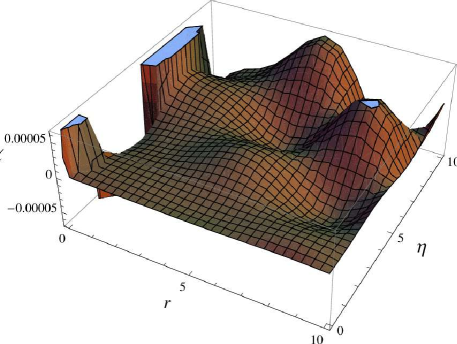
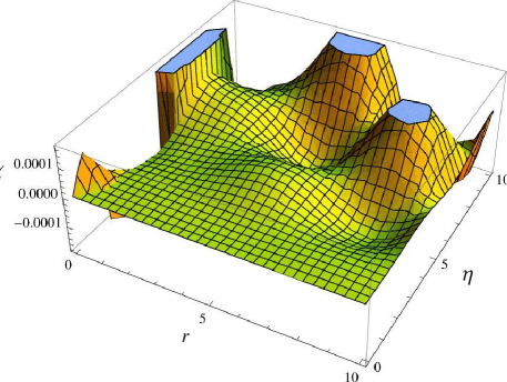
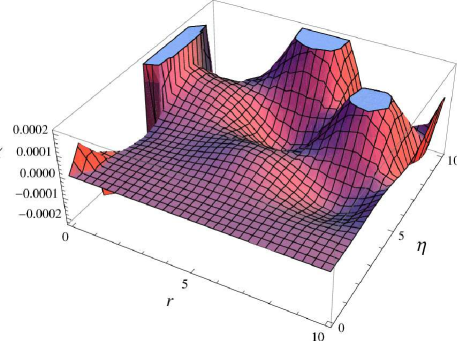
Figure 1: Plots of $\chi$ versus $r$ and $\eta$ for $A_{1}=-1$, $c_{3}=0.01$, $c_{4}=0.01$, $c_{5}=0.01$, $c_{6}=0.01$, $\lambda=0$ (brown), $\lambda=3(1+\sqrt{5})\pi$ (yellow) and $\lambda=3(1+\sqrt{5})\pi$ (pink).

To find the remaining metric perturbation coefficient $\varphi$, we consider the speed of sound formula $v_{s}^{2}=\frac{\partial p}{\partial\rho}$ which gives $\Delta\rho_{0}=\Pi p_{0}$. Using this relation (between $\Delta$ and $\Pi$) and then comparing Eqs.(24), (25), we have

$$-2A_{3}\varphi^{\prime\prime}+2A_{4}\ddot{\varphi}+(6A_{3}-2A_{4})\dot{\varphi}H-\frac{4A_{3}}{r}\varphi^{\prime}+\left\{A_{3}\left(\frac{12}{r^{2}}-6H^{2}\right)\right.$$

$$\left.-2H^{2}A_{4}\right\}\varphi+\frac{2}{r}(A_{3}-A_{4})\chi^{\prime}+2H(A_{3}+A_{4})\dot{\chi}+\left\{A_{3}\left(-\frac{4}{r^{2}}+2H^{2}\right)\right.$$

$$\left.-A_{4}\left(\frac{2}{r}-\frac{4}{r^{2}}-4\dot{H}+2H^{2}\right)\right\}\chi-4HA_{3}\sigma^{\prime}-\frac{8H}{r}A_{3}\sigma=0,$$ (40)

with $A_{3}=8\pi v_{s}^{2}+(3v_{s}^{2}-1)\lambda$ and $A_{4}=8\pi+(3-v_{s}^{2})\lambda$. Replacing the values of $\chi$ and $\sigma$ in the above equation, we can obtain the evolution equation of $\varphi$ which will be a hyperbolic differential equation and may be solved using some suitable initial as well as boundary conditions. The first two perturbed field equations describe the evolution of matter fluctuations and the last two can depict the disturbances in velocity components. All these evolution equations for perturbation parameters contain the curvature-matter coupling parameter $\lambda$ implying that their evolution will be affected by $\lambda$. To observe the effects of coupling on the propagation of GWs, we plot the metric perturbation parameter $\chi$ for three different values of $\lambda$ as shown in Figure 1. The constant $A_{1}$ is related with $\lambda$ via the relation $A_{1}=\frac{6\pi+2\lambda}{6\pi+\lambda}-\left(\frac{6\pi+2\lambda}{6\pi+\lambda}\right)^{2}$. Thus we choose the value of $A_{1}$ such that the corresponding value of $\lambda$ lies in the range $\lambda>-4\pi$ which comes from the viability or stability criteria for any $f(R,T)$ gravity model [53]. For the assumed values of all constants as well as ranges of independent parameters, the maximum amplitude of wave is approximately $0.00005$ for $\lambda=0$ (GR case), $0.0001$ for $3(1+\sqrt{5})\pi$ and $0.0002$ for $6(1+\sqrt{5})\pi$. It can easily be noted that the increase in the value of $\lambda$ causes an increase in the maximal amplitude of GW.

Now, we extend our discussion for dark energy dominated phase of cosmic evolution. For this purpose, we substitute the EoS $p_{0}=-\rho_{0}$ in the field equations and obtain the following evolution equations

$$-2\varphi^{\prime\prime}-\frac{4}{r}\varphi^{\prime}+6H\dot{\varphi}-6H^{2}\varphi+2\frac{l(l+1)}{r^{2}}\varphi+\frac{2}{r}\chi^{\prime}+2H\dot{\chi}+\frac{2\chi}{r^{2}}+2\chi H^{2}$$

$$-\frac{l(l+1)}{r^{2}}\chi-4H\sigma^{\prime}-\frac{8H}{r}\sigma=2a^{4}[(8\pi+3\lambda)\Delta+\lambda\Pi]\rho_{0},$$ (41)

$$-2\ddot{\varphi}+2H\dot{\varphi}+2H^{2}\varphi-2H\dot{\chi}+\frac{2\chi^{\prime}}{r}+\frac{\chi}{r^{2}}[l(l+1)-2]-4\dot{H}\chi+2H^{2}\chi$$

$$=-2a^{4}[(8\pi+3\lambda)\Pi+\lambda\Delta]\rho_{0},$$ (42)

$$\chi^{\prime}=\dot{\sigma},$$ (43)

$$-\frac{\ddot{\chi}}{2}-\frac{\chi^{\prime\prime}}{2}-\frac{\chi^{\prime}}{r}+\chi(H^{2}-\dot{H})-\ddot{\varphi}+H\dot{\varphi}+H^{2}\varphi+\dot{\sigma}^{\prime}+\frac{\dot{\sigma}}{r}$$

$$=-a^{4}[(8\pi+3\lambda)\Pi+\lambda\Delta]\rho_{0},$$ (44)

$$2\dot{\varphi}^{\prime}+2H\varphi^{\prime}+2H\chi^{\prime}-\frac{2}{r}\dot{\chi}+\frac{4H\chi}{r}-2H^{2}\sigma-\frac{l(l+1)}{r}\sigma=0,$$ (45)

$$2\dot{\varphi}-2H\varphi+\dot{\chi}-\sigma^{\prime}=0,$$ (46)

Here, the Hubble parameter and background density have the following expressions

$$H(\eta)=\frac{1}{\hat{c}_{1}-\eta},\quad\rho_{0}=\frac{3}{4(2\pi+\lambda)\hat{c}_{2}},$$

with $\hat{c}_{1}$ and $\hat{c}_{2}$ as constants of integration. Equation (44) yields the same evolution equation for $\chi$ as in the radiation era. Consequently, we have the same expressions for the metric perturbation parameters $\chi$ and $\sigma$ (for $\hat{c}_{1}=0$) with $A_{1}=-2$. We also find the expression of $\varphi$ from Eq.(46) but that is too much lengthy to present here. The expressions of $\Delta$ and $\Pi$ can be found from Eqs.(41) and (42). However, the velocity perturbation parameters do not appear in these field equations.

4 Concluding Remarks

Gravitational waves are the outcome of some cosmic events such as big bang, gravitational collapse and mergence of two black holes or ultra dense neutron stars. These waves flow over the Earth continuously but our instruments are not yet too sensitive to detect most of them individually. A very few of these signals that can be assigned to a single event have been observed by the latest laser interferometers. These collisions of compact objects also produce stochastic background of GWs and advanced LIGO-Virgo interferometers are sensitive to these signals with a certain frequency and wave amplitude [54]. If the GW causes a displacement in the initial positions (i.e., the positions before passing the GW) of freely falling particles which remains permanently after the GW passed, we speak of the GW memory effect. A GW without this effect can cause an oscillatory deformation in a detector while with memory effect can cause a permanent deformation in a true free falling detector [55].

Gravitational waves have also been studied extensively in modified theories of gravity. It is expected that the Earth based network of interferometers could provide constraints for these theories by analyzing different properties of GWs. Cai et al. [56] and Li et al. [57] discussed some constraints for teleparallel theory using the effective field theory approach. Gong et al. [58] worked out to constrain the scalar tensor theory in view of recent GW observations.

This paper investigates the propagation of polar GWs in $f(R,T)$ theory of gravity. The polar GWs are assumed by perturbing the flat FRW metric through polar (or even) waves in Regge-Wheeler gauge. The corresponding matter and four velocity are also perturbed such that the four velocity may be non-comoving. We find the perturbing parameters via the field equations. The evolution equation of $\chi$ is a wave equation yielding its value (LABEL:s11) which in turn gives $\sigma$ (39). Equation (40) leads to a hyperbolic differential equation in $\varphi$ after replacing the expressions of $\chi$ and $\sigma$. This can be solved using suitable initial and boundary conditions as well as choosing appropriate free parameters. The parameters $v$ and $w$ can be explicitly obtained from Eqs.(28) and (29) while $u$ vanishes.

All the equations as well as obtained expressions have the terms involving model parameter $\lambda$ indicating that the curvature-matter coupling affect the evolution of perturbation parameters and consequently the propagation of polar waves in radiation dominated era. We have also investigated the propagation of polar waves in dark energy dominated universe. It is observed that the increase in $\lambda$ can enhance wave amplitude, i.e., we can expect GWs with higher amplitudes if the value of curvature-matter coupling constant increases. The analysis of observed GW signals by LIGO-VIRGO collaboration shows that masses of the merging black holes are directly related with energy radiated by the coalesce as well as the amplitude of resulting GW. For $f(R,T)=R+2\lambda T$ gravity model, it has also been observed that if the value of $\lambda$ is increased, it increases the mass range of the corresponding compact object [21, 25]. Moreover, when these compact objects are in binaries and their mergence produces GWs then the massive objects produce GWs of greater amplitude. Hence our conclusion that amplitude increases with $\lambda$ is in agreement with the literature.

In GR [45], it is proved that vanishing of material perturbations lead to vanishing of polar GWs, i.e., if polar waves are passing through the spacetime the corresponding mater must also be perturbed. In the absence of material perturbations, i.e., for $\Delta=\Pi=v=w=0$ we obtain the same perturbed field equations as in GR. The only difference is in the value of $H$ which has no impact on the above mentioned fact. Thus, we can conclude that for $f(R,T)=R+2\lambda T$ gravity model, there are no polar GWs when there are no matter perturbations which is consistent with GR.

For axial waves, we have found the expressions of perturbation parameters which show the effect of $f(R,T)=R+2\lambda T$ gravity on the propagation of axial GW [50]. To find these perturbations, we use the constraint that matter perturbations vanish for axial waves which are originally non-zero in $f(R,T)$ gravity in contrast to GR. However, for polar waves, such an assumption leads to vanishing of polar GWs. For polar waves, we have checked the effects of $R+2\lambda T$ gravity model by plotting the metric perturbation function $\chi$ for different values of $\lambda$.

Acknowledgment

One of us (AS) would like to thank the Higher Education Commission, Islamabad, Pakistan for its financial support through the Indigenous Ph.D. 5000 Fellowship Program Phase-II, Batch-III.

References

- [1] Buchdahl, H. A.: Mon. Not. R. Astron. Soc. 150(1970)1.
- [2] Nojiri, S. and Odintsov, S.D.: Phys. Lett. B 631(2005)1.
- [3] Harko, T., Lobo, F.S.N., Nojiri, S. and Odintsov, S.D.: Phys. Rev. D 84(2011)024020.
- [4] Ratra, P. and Peebles, L.: Phys. Rev. D 37(1988)3406.; Caldwell, R.R., Dave, R. and Steinhardt, P.J.: Phys. Rev. Lett. 80(1998)1582.
- [5] Kamenshchik, A.Yu, Moschella, U. and Pasquier, V.: Phys. Lett. B 511(2001)265; Bento, M.C., Bertolami, O. and Sen, A.A.: Phys. Rev. D 66(2002)043507.
- [6] Caldwell, R.R.: Phys. Lett. B 545(2002)23.
- [7] Afshordi, N., Chung, D.J.H. and Geshnizjani, G.: Phys. Rev. D 75(2007)083513.
- [8] Setare, M.R.: Phys. Lett. B 648(2007)329; ibid. 653(2007)116.
- [9] Cai, Y.F., Capozziello, S., De Laurentis, M. and Saridakis, E.N.: Rept. Prog. Phys. 79(2016)106901.
- [10] Jamil, M. et al.: Eur. Phys. J. C 72(2012)1999.
- [11] Houndjo, M.J.S.: Int. J. Mod. Phys. D 21(2012)1250003.
- [12] Sharif, M. and Nawazish, I.: Eur. Phys. J. C 77(2017)198.
- [13] Sharif, M. and Siddiqa, A.: Mod. Phys. Lett. A 32(2017)1750151.
- [14] Sharif, M. and Siddiqa, A.: Commun. Theor. Phys. 69(2018)537.
- [15] Sharif, M. and Zubair, M.: J. Cosmol. Astropart. Phys. 03(2012)028.
- [16] Jamil, M., Momeni, D. and Myrzakulov, R.: Chin. Phys. Lett. 29(2012)109801.
- [17] Sharif, M. and Zubair, M.: Exp. Theor. Phys. 117(2013)248,
- [18] Momeni, D., Moraes, P.H.R.S. and Myrzakulov R.: Astrophys. Space Sci. 361(2016)228.
- [19] Noureen, I. and Zubair, M.: Astrophys. Space Sci. 356(2015)103.
- [20] Zubair, M., Abbas, G. and Noureen, I.: Astrophys. Space Sci. 361(2016)8.
- [21] Moraes, P.H.R.S., Jos D.V.A. and Malheiro, M.: J. Cosmol. Astropart. Phys. 06(2016)005.
- [22] Sharif, M. and Waseem, A.: Can. J. Phys. 94(2016)1024.
- [23] Carvalho, G.A. et al.: Eur. Phys. J. C 77(2017)871.
- [24] Yousaf, Z., Bhatti, M.Z. and Ume Farwa: Class. Quantum Grav. 34(2017)145002.
- [25] Sharif, M. and Siddiqa, A.: Eur. Phys. J. Plus 132(2017)529.
- [26] Sharif, M. and Siddiqa, A.: Int. J. Mod. Phys. D 27(2018)1850065.
- [27] Zubair, M., Waheed, S. and Ahmad, Y.: Eur. Phys. J. C 76(2016)444.
- [28] Moraes, P.H.R.S. and Sahoo, P.K.: Phys. Rev. D 96(2017)044038.
- [29] Zubair, M., G. Mustafa, Waheed, S. and Abbas, G.: Eur. Phys. J. C 77(2017)680.
- [30] Sahoo, P.K., Moraes, P.H.R.S. and Sahoo, P.: Eur. Phys. J. C 78(2018)46.
- [31] Abbott, B.P. et al.: Phys. Rev. Lett. 116(2016)061102.
- [32] Abbott, B.P. et al.: Phys. Rev. Lett. 118(2017)221101.
- [33] Abbott, B.P. et al.: Phys. Rev. Lett. 119(2017)161101.
- [34] Kausar, H.R., Philippoz, L. and Jetzer, P.: Phys. Rev. D 93(2016)124071.
- [35] Sharif, M. and Siddiqa, A.: Astrophys. Space Sci. 362(2017)226.
- [36] Alves, M.E.S., Moraes, P.H.R.S., de Araujo, J.C.N. and Malheiro, M.: Phys. Rev. D 94(2016)024032.
- [37] Sharif, M. and Siddiqa, A.: Phys. Dark Universe 15(2017)105.
- [38] Regge, T. and Wheeler, J.A.: Phys. Rev. 108(1957)1063.
- [39] Zerilli, F.J.: Phys. Rev. D 02(1970)2141.
- [40] Malec, E. and Wylȩżek, G.: Class. Quantum Grav. 22(2005)3549.
- [41] Stewart, J.M., Walker, M.: Proc. R. Soc. Lond. A 341(1974)49.
- [42] Keresztes, Z., Forsberg, M., Bradley, M., Dunsby, P.K.S. and Gergely, L.A.: J. Cosmol. Astropart. Phys. 2015(2015)042.
- [43] Bradley, M., Forsberg, M. and Keresztes, Z.: Universe 3(2017)69.
- [44] Viaggiu, S.: Class. Quantum Grav. 34(2017)035018.
- [45] Kulczycki, W. and Malec, E.: Class. Quantum Grav. 34(2017)135014.
- [46] Kulczycki, W. and Malec, E.: Phys. Rev. D 96(2017)063523.
- [47] Gerlach, U.H. and Sengupta, U.K.: Phys. Rev. D 19(1979)2268; ibid. 22 (1980)1300.
- [48] Gundlach, C. and Martin-Garcia, J.M.: Phys. Rev. D 61(2000)084024.
- [49] Clarkson, C., Clifton, T. and February, S.: J. Cosmol. Astropart. Phys. 06(2009)25.
- [50] Sharif, M. and Siddiqa, A.: Eur. Phys. J. C 78(2018)721.
- [51] Poplawski, N.J.: arXiv:gr-qc/0608031.
- [52] Faraoni, V.: Phys. Rev. D 80(2009)124040.
- [53] Haghani, Z., Harko, T., Lobo, F.S.N., Sepangi, H.R. and Shahidi, S.: Phys. Rev. D 88(2013)044023; Sharif, M. and Zubair, M.: Astrophys. Space Sci. 349(2014)529.
- [54] Abbott, B.P. et al.: Phys. Rev. Lett. 120(2018)091101.
- [55] Favata, M.: Class. Quantum Grav. 27(2010)084036.
- [56] Cai, Y.F., Li, C., Saridakis, E.N. and Xue, L.: Phys. Rev. D 97(2018)103513.
- [57] Li, C., Cai, Y., Cai, Y.F. and Saridakis, E.N.: J. Cosmol. Astropart. Phys. 10(2018)001.
- [58] Gong, Y., Papantonopoulos, E. and Yi, Z.: Eur. Phys. J. C 78(2018)738.