Abstract

We introduce in this paper an equivalence notion for submersions $U\to\mathbb{R}$, $U$ open in $\mathbb{R}^{2}$, which makes it possible to identify a smooth planar curve with a unique class of submersions. This idea, which extends to the nonlinear setting the construction of a dual projective space, provides a systematic way to handle global implicit descriptions of smooth planar curves. We then apply this framework to model nonlinear electrical devices as classes of equivalent functions. In this setting, linearization naturally accommodates incremental resistances (and other analogous notions) in homogeneous terms. This approach, combined with a projectively-weighted version of the matrix-tree theorem, makes it possible to formulate and address in great generality several problems in nonlinear circuit theory. In particular, we tackle unique solvability problems in resistive circuits, and discuss a general expression for the characteristic polynomial of dynamic circuits at equilibria. Previously known results, which were derived in the literature under unnecessarily restrictive working assumptions, are simply obtained here by using dehomogenization. Our results are shown to apply also to circuits with memristors. We finally present a detailed, graph-theoretic study of certain stationary bifurcations in nonlinear circuits using the formalism here introduced.

Keywords: planar curve, projective space, homogeneous coordinates, matrix-tree theorem, nonlinear circuit, memristor, characteristic polynomial, equilibrium point, bifurcation.

1 Introduction

Implicit descriptions are often used at the initial stages in dynamical system modelling within many branches of science and engineering. Incidentally, implicit systems of differential-equations, also termed differential-algebraic systems or singular systems, have become a widely used tool in system modelling, with different names depending on the application field: e.g. DAEs are termed semistate systems in circuit modelling, descriptor systems in control theory, or constrained systems in mechanics [2, 19, 20, 27, 29]. Much research has been focused on numerical methods directed to such implicit descriptions: see [2, 19, 20, 28].

However, from an analytical perspective, it is common to renounce such implicit formulations at a relatively early stage of the aforementioned modelling process, in particular in the formulation of reduced-order models. This is the case when using local coordinates for the description of the manifold where trajectories lie, within the aforementioned differential-algebraic framework. Alternatively, one can restrict the scope of the analysis to cases in which such a manifold admits a global coordinate description. The price we pay for this is of course a loss of generality.

The circuit context provides clear examples of this. Focusing for instance on a nonlinear resistor (a device defined by a nonlinear characteristic relating voltage and current), it is very common to assume that this characteristic either has a global current-controlled form or a global voltage-controlled form, i.e. that it can be written either as $v=h(i)$ or as $i=g(v)$ for appropriate, globally defined functions $h$ or $g$. Analogous remarks apply for other types of devices. In many cases such restrictions make perfect sense because of physical reasons but, at the risk of being too sketchy, from a mathematical point of view they may also reflect the fact that the available concepts and tools are mainly directed to such restricted contexts. Keeping a fully-implicit form (that is, working with a general implicit characteristic $f(i,v)=0$ throughout the analysis, to continue with the example above) often involves additional difficulties or is simply unfeasible. The reader is referred to subsection 3.2.1 for a more detailed discussion of this. Regardless of the reasons, it is clear that such a loss of generality is important from a theoretical point of view and may also be relevant in many practical contexts, in particular in qualitative studies of nonlinear systems (including e.g. global bifurcation analyses).

Surprisingly, such unnecessarily restrictive assumptions often occur in the simplest linear problems. In the circuit context, when writing Ohm’s law for a linear resistor as $v=zi$ or $i=yv$ (we use the common notations $z$, $y$ for the impedance and the admittance parameters, which take complex values; the reader may also think of resistance and conductance in the real domain) some cases are necessarily left out; indeed, the form $v=zi$ does not accommodate an open-circuit, whereas $i=yv$ excludes a short-circuit. The idea, of course, is to treat $z$ or $y$ as symbolic variables in general parametric analyses, not focusing on specific numerical values. To this aim, we might consider using a fully-implicit description of a linear resistor or an impedance, by writing such a characteristic in the general form

$$pv-qi=0,$$ (1)

with the only requirement that the parameters $p$ and $q$ do not vanish simultaneously. As detailed in subsection 2.1, it is natural to think of $(p:q)$ as homogeneous coordinates of a point in a (real or complex) projective line, with the invariant ratios $y=p/q$ and $z=q/p$ defined on the corresponding subsets of the parameter space. The key idea is to look at the left-hand side of (1), with fixed values of $p$ and $q$, only as a representative of a family of equivalent forms, which are defined up to a non-vanishing constant (as in the standard construction of the projective space from a given vector space, in this case the space of linear forms $L(\mathbb{K}^{2},\mathbb{K})$, with $\mathbb{K}=\mathbb{R}$ or $\mathbb{C}$). This way we identify a linear resistor with an equivalence class of linear forms and we are naturally led to a projective context. This supports a projective-based formalism to set up linear circuit models in broadly general terms, as detailed in [32].

In this context, the present paper is driven by a two-fold goal. Our first purpose is to set the foundations for the extension of this approach to the nonlinear setting. This is a purely mathematical problem, independent of the application field. Using ideas from sheaf theory, we will extend in Section 2 the projective-based approach above in order to describe smooth planar curves as classes of equivalent functions; here the equivalence notion will not rely on the one supporting the construction of a projective space, as indicated for (1) above, but extends this idea using the notion of associate submersions (we borrow the “associate” term from the polynomial context). This provides a nice setting to handle systematically global implicit descriptions of planar curves. Linearization at a given point of the characteristic curve will naturally define a linear form fitting the projective context mentioned above. We believe these ideas to be of independent mathematical interest and of potential use in different branches of applied mathematics, science and engineering.

The formalism above can be naturally combined with determinantal, graph-theoretic tools [6, 7] to address in broad generality certain qualitative aspects of nonlinear circuits. This is the second goal of the paper, which is tackled in Sections 3 and 4. Following the philosophy of [11, 31], but using very different tools, we will characterize in graph-theoretic terms different analytical properties of nonlinear circuits, involving e.g. the unique solvability of nonlinear resistive circuits or certain bifurcations of equilibria in a dynamic context. We will also derive a general expression for the characteristic polynomial of a nonlinear circuit at equilibrium, in terms of the structure of spanning trees. All these results hold under a fully-implicit form for resistors (and memristors, when present). A key result in our approach, proved in [32], is a projectively-weighted version of the matrix-tree theorem. This result makes it possible to exploit the homogeneous form of the incremental resistances and memristances to address in an implicit context the problems mentioned above, without the need to resort to (local or global) explicit descriptions of the corresponding devices. We consider in more detail a bifurcation problem in Section 4 where, specifically, we use our framework to provide a graph-theoretic characterization of so-called simple stationary bifurcation points in nonlinear circuits. Finally, the reader can find some concluding remarks in Section 5. Throughout the paper, several examples illustrate the results.

2 Associate submersions

In this section we address the following problem. From elementary linear algebra we know that a straight line through the origin in the real plane can be described as the kernel of a nontrivial linear form, that is, a nonzero element of $L(\mathbb{R}^{2},\mathbb{R})$. Moreover, all such linear forms can be identified as equivalent in terms of a standard relation, namely, the one defining a projective space from a given vector space. Consider now the nonlinear version of this problem: given a smooth curve in the plane, can we describe it as a zero set of a globally defined function? Provided that this is the case (this actually follows from well-known results in differential geometry), may all such functions be made equivalent in some sense? We tackle this in what follows. By way of motivation, we present in advance further details of the problem in the linear context in electrical circuit terms.

2.1 Motivation: linear devices as points in a projective line

As indicated in Section 1, following [32] we look at the characteristic of a given linear electrical device as the kernel of a linear form or, more precisely, as the common kernel of all linear forms from a certain equivalence class. Specifically, in the vector space of linear forms $\mathbb{R}^{2}\to\mathbb{R}$ (with the standard operations) we identify two non-null forms $f$, $g$ as equivalent if there exists a (non-zero) constant $\mu$ such that

$$f=\mu g.$$ (2)

In the circuit context, a linear resistor will be a point in the resulting quotient space, that is, an equivalence class of linear forms.

This construction defines a real projective line. Fix now the attention on a resistor defined by a characteristic such as (1) and let $f(i,v)$ stand for the left-hand side of this equation. By means of the basis defined by $f_{1}(i,v)=v$ and $f_{2}(i,v)=-i$ we may understand the parameters $p$, $q$ to define homogeneous coordinates in the aforementioned projective line, since $(p:q)$ is the pair for which the identity $f(i,v)=pf_{1}(i,v)+qf_{2}(i,v)$ holds. If we multiply the left-hand side of (1) by a non-null constant, this constant arises as a common factor to both parameters $p$ and $q$, so that the ratio is the same: this makes the homogeneous nature of the pair clear. Such a coordinate pair $(p:q)$ is called a homogeneous description of the resistance.

The advantage of this formalism is of course its generality. Regardless of the choice of a specific pair of homogeneous coordinates or, in other terms, of the choice of a particular linear form within the equivalence class defining the resistor, the (say, classical) resistance $q/p$ and the conductance $p/q$ are well-defined and unique in the so-called current-controlled and voltage-controlled affine patches defined by the conditions $p\neq 0$ and $q\neq 0$, respectively. The point is that by using the projective formalism we do not need to restrict the analysis to such patches, and this idea may in principle apply throughout the whole of linear circuit theory. The same holds for the impedance and the admittance in the complex domain. A detailed discussion, focusing on the formulation of reduced models, can be found in [32]. We refer the reader to [4, 5, 25, 34] for some related approaches.

2.2 Nonlinear devices as equivalence classes of associate submersions

2.2.1 Global description of planar curves

Our first goal in this paper is to extend this modeling approach to the nonlinear context. To do so, we introduce in what follows a formalism to describe smooth planar curves as classes of equivalent functions; the equivalence notion will not rely on the one supporting the projective construction above, but extends this idea using the notion of associate submersions (recall that a submersion is a smooth map with a surjective differential everywhere). Linearization at a given point of the curve will naturally define a linear form fitting the projective context of subsection 2.1. We will exploit these notions in the electrical circuit context in later sections but, for the sake of generality, in the remainder of this one we work with abstract curves and functions.

All maps and manifolds will be (often implicitly) assumed to be $C^{\infty}$, so that “smooth” means $C^{\infty}$, even if this could be relaxed at many points. The attention is focused on smooth, connected 1-manifolds in $\mathbb{R}^{2}$, which for brevity will be termed smooth planar curves. We adopt the usual notion for manifolds in Euclidean space, defining them as regular submanifolds of $\mathbb{R}^{n}$ by assuming the existence of adapted charts (find this e.g. in [38, Definition 9.1]). This amounts to requiring that each point of the curve, with the topology inherited from $\mathbb{R}^{2}$, has a neighborhood diffeomorphic to a real interval [21]. We do not assume that the curves define closed subsets of $\mathbb{R}^{2}$.

Regular submanifolds are well-known to admit local descriptions as level sets of submersions (see [21, Proposition 5.16]). Our first remark is that for planar curves the same kind of description is also feasible in a global sense.

Proposition 1.

Any smooth planar curve admits a global description as the zero set of a smooth submersion defined on some open subset of  $\mathbb{R}^{2}$.

Even if it is not easy to find an explicit statement of this claim in the literature, it is a straightforward combination of two well-known facts in differential geometry, namely: that an orientable codimension-one manifold (hypersurface) in $\mathbb{R}^{n}$ is the zero set of a submersion $U\to\mathbb{R}$ for some open set $U$ including the hypersurface (an explicit statement can be found for instance in [35]), and that 1-dimensional manifolds are orientable (see e.g. [21]).

This means that an implicit description $f(x)=0$ of a smooth planar curve ${\cal C}$ holds in a global sense, with $f$ defined on some open neighborhood $U$ of ${\cal C}$; such a function $f:U\to\mathbb{R}$ is called a global defining function for ${\cal C}$. Note that in general $U$ need not be the whole plane $\mathbb{R}^{2}$, although if the curve is diffeomorphic to $\mathbb{S}^{1}$ then it can indeed be described as the zero set of a submersion defined on $\mathbb{R}^{2}$, as a consequence of the smooth Jordan-Schöenflies theorem.

2.2.2 Equivalence classes of associate submersions

It is clear that there are infinitely many submersions defining a given smooth curve ${\cal C}$. Our present purpose is to provide a formal definition making all of them equivalent and extending the aforementioned projective-based construction, which only applies to linear problems. The difficulty in the nonlinear case relies on the fact that the submersions eventually defining a zero set do not need to share a common domain, contrary to linear forms which are well-defined on the whole of $\mathbb{R}^{2}$; moreover, since ${\cal C}$ is not fixed a priori there is no chance to localize the definition on a neighborhood of the curve, as it is done for instance to define germs. Sheaves naturally arise here, since this notion accommodates families of functions defined on open subsets of a given topological space without restricting a priori a common domain for all of them. We refer the reader to [14] for general background on sheaf theory. For our purposes it is enough to consider the sheaf of submersions ${\cal S}$ (which is a sheaf of sets, cf. [14]) as the family of all pairs $(f,U)$ with $U$ an open set of $\mathbb{R}^{2}$ and $f:U\to\mathbb{R}$ a smooth submersion. In this context, the following definition will capture the sought correspondence between smooth planar curves and classes of global defining functions (cf. Theorem 1).

Definition 1.

Two smooth submersions $f_{1}$, $f_{2}$, defined respectively on open subsets $U_{1}$, $U_{2}$ of $\mathbb{R}^{2}$, are said to be associates if the following two conditions hold.

1. If $U_{1}\neq U_{2}$, then $f_{i}\neq 0$ on $U_{i}-U_{j}$, for $\{i,j\}=\{1,2\}$.

2. If $U=U_{1}\cap U_{2}\neq\emptyset$, then there exists a nowhere zero smooth function $\gamma:U\to\mathbb{R}$ such that $f_{1}=\gamma f_{2}$ holds on the whole of $U$.

Proposition 2.

The relation of being associates is an equivalence relation in the sheaf ${\cal S}$.

Proof. The fact that the relation is reflexive and symmetric is clear. We need to show that it is also transitive. To this end, denote the relation by $\sim$ and suppose $(f_{1},U_{1})\sim(f_{2},U_{2})$ and $(f_{2},U_{2})\sim(f_{3},U_{3})$. We prove in what follows that $(f_{1},U_{1})\sim(f_{3},U_{3})$.

We first need to check that $f_{1}\neq 0$ on $U_{1}-U_{3}$ (for $f_{3}$ the reasoning is symmetrical). Split this set as $U_{1}-U_{3}=[U_{1}-(U_{2}\cup U_{3})]\cup[(U_{1}\cap U_{2})-U_{3}].$ The first set in the right-hand side is a subset of $U_{1}-U_{2}$ and therefore $f_{1}\neq 0$ there. The second one is a subset of $U_{1}\cap U_{2}$, where the identity $f_{1}=\gamma_{12}f_{2}$ holds for some nowhere zero function $\gamma_{12}$, and it is also a subset of $U_{2}-U_{3}$, where $f_{2}$ is known not to vanish: we conclude that $f_{1}=\gamma_{12}f_{2}$ is not zero there, either, and the first part of the proof is complete.

We also need to show that if $U_{1}\cap U_{3}$ is non-empty, then there exists a nowhere zero, smooth function $\gamma_{13}$ such that $f_{1}=\gamma_{13}f_{3}$ there. Write $U_{1}\cap U_{3}=[U_{1}\cap U_{2}\cap U_{3}]\cup[(U_{1}\cap U_{3})-U_{2}]$ and note that on the first we set may write $f_{1}=\gamma_{12}\gamma_{23}f_{3}$, where $\gamma_{23}$ is nowhere zero and such that $f_{2}=\gamma_{23}f_{3}$ on $U_{2}\cap U_{3}$. Let us then define

$$\gamma_{13}(x)=\begin{cases}\gamma_{12}(x)\gamma_{23}(x)&\text{ if }x\in U_{1}\cap U_{2}\cap U_{3}\vspace{1mm}\\ f_{1}(x)/f_{3}(x)&\text{ if }x\in(U_{1}\cap U_{3})-U_{2}.\end{cases}$$ (3)

Be aware that the quotient here is well-defined because $f_{3}$ does not vanish on $U_{3}-U_{2}$, which includes $(U_{1}\cap U_{3})-U_{2}$. Note also that the identity $f_{1}=\gamma_{13}f_{3}$ holds trivially in light of the definition of $\gamma_{13}$. The function $\gamma_{13}$ so defined does not vanish because, on the one hand, neither $\gamma_{12}$ nor $\gamma_{23}$ do on $U_{1}\cap U_{2}\cap U_{3}$ and, on the other, $f_{1}$ is non-null on $(U_{1}\cap U_{3})-U_{2}\subseteq U_{1}-U_{2}$. Finally, $\gamma_{13}$ is smooth; this is clear for any $x\in U_{1}\cap U_{2}\cap U_{3}$ because this is an open set and $\gamma_{13}$ is a product of smooth functions there; for $x\in(U_{1}\cap U_{3})-U_{2}$, smoothness follows from the fact that $f_{3}$ does not vanish on this set, and by construction $\gamma_{13}$ equals the smooth quotient $f_{1}/f_{3}$ on some open neighborhood of $x$. $\Box$

Theorem 1.

Two smooth submersions from the sheaf ${\cal S}$ defined above yield the same zero set if and only if they are associates.

Proof. The “if” part of the claim directly follows from Definition 1. For the “only if” part, what we need to show is that, if $f_{1},$ $f_{2}$ are two submersions with open domains $U_{1}$, $U_{2}$ and defining the same zero set ${\cal C}$, there exists a nowhere zero smooth function $\gamma:U\to\mathbb{R}$ defined on the intersection $U=U_{1}\cap U_{2}$ such that

$$f_{1}=\gamma f_{2}$$ (4)

on $U$. To do this, let us first fix $x^{*}\in{\cal C}$. Since by definition $f_{2}$ is a submersion, the differential $(df_{2})_{x^{*}}$ is surjective and this implies that at least one of the partial derivatives ${f_{2}}_{x_{i}}$ does not vanish (for brevity, we write $x_{i}$ as a subscript to denote partial differentiation). Assume w.l.o.g. that the first partial derivative ${f_{2}}_{x_{1}}$ is not zero at $x^{*}$, and define a local coordinate change by the local diffeomorphism $y=\alpha(x)$ given by $y_{1}=f_{2}(x)$, $y_{2}=x_{2}$. Denote the inverse of $\alpha$ as $\beta$, so that $x=\beta(y)$. Then we have $f_{2}(\beta(y))=y_{1}$ and, by the hypothesis that $f_{1}$ and $f_{2}$ define the same zero set, we have (always in a local sense) $f_{1}(\beta(y))=0$ iff $y_{1}=0$. According to Hadamard’s lemma (see e.g. [12]), it follows that $f_{1}(\beta(y))$ can be written as $f_{1}(\beta(y))=\kappa(y)y_{1}$ for some locally defined function $\kappa$. In $x$-coordinates the latter relation reads as $f_{1}(x)=\kappa(\alpha(x))f_{2}(x),$ so that $\kappa\circ\alpha$ yields a locally defined function, say $\gamma^{x^{*}}$, for which the identity $f_{1}(x)=\gamma^{x^{*}}(x)f_{2}(x)$ holds on some neighborhood of $x^{*}$.

To check that $\gamma^{x^{*}}$ does not vanish at $x^{*}$ (and hence on a sufficiently small neighborhood of this point) it is enough to use $f_{2}(x^{*})=0$ in order to derive $(df_{1})_{x^{*}}=\gamma^{x^{*}}(x^{*})(df_{2})_{x^{*}}$ by Leibniz’s rule. The fact that $df_{1}$ is surjective at $x^{*}$ implies $\gamma^{x^{*}}(x^{*})\neq 0$, as claimed.

To finish the proof, we define $\gamma$ globally on the intersection $U=U_{1}\cap U_{2}$ as

$$\gamma(x)=\begin{cases}f_{1}(x)/f_{2}(x)&\text{ if }f_{2}(x)\neq 0\\ \gamma^{x}(x)&\text{ if }f_{2}(x)=0,\end{cases}$$ (5)

which obviously does not vanish and meets the requirement depicted in (4) (recall that we are assuming $f_{1}$ and $f_{2}$ to define the same zero set). One can easily check that $\gamma$ is smooth because, for any $x^{*}\in{\cal C}$, the function $\gamma(x)$ equals the locally defined one $\gamma^{x^{*}}(x)$ on some neighborhood of $x^{*}$; indeed, for any $x\in{\cal C}$ sufficiently close to $x^{*}$, the prescribed value $\gamma^{x}(x)$ must equal $\gamma^{x^{*}}(x)$ because $\gamma^{x}$ and $\gamma^{x^{*}}$ coincide, by construction, in the open and dense subset defined by the condition $f_{2}(x)\neq 0$ on the intersection of their domains. $\Box$

Theorem 1 yields a one-to-one correspondence between smooth planar curves and equivalence classes of global defining functions, since we have shown that two submersions $f_{1}$, $f_{2}$ define the same zero set if and only if a relation of the form $f_{1}=\gamma f_{2}$ holds for some nowhere-zero function $\gamma$ defined on an open neighborhood of this zero set.

2.3 Linearization

Linearization at a given point naturally amounts to the projective construction of subsection 2.1. Indeed, fix any submersion $f_{1}$ defining a smooth planar curve ${\cal C}$. The differential of $f_{1}$ at any given $x\in{\cal C}$ defines the linear form $(df_{1})_{x}:\mathbb{R}^{2}\to\mathbb{R}$ (mind the canonical identification $T_{x}\mathbb{R}^{2}\sim\mathbb{R}^{2}$). Following the construction in Theorem 1 (cf. (4)), and using the property $f_{2}(x)=0$ for $x\in{\cal C}$, $f_{2}$ being any other submersion defining ${\cal C}$, we derive $(df_{1})_{x}=\gamma(x)(df_{2})_{x}$ with $\gamma(x)\neq 0$: therefore, $(df_{1})_{x}$ and $(df_{2})_{x}$ are equivalent linear forms in the projective sense indicated in subsection 2.1. Geometrically, the remarks above simply express that the common kernel of all these differentials characterizes the tangent space to the curve at $x$.

It is worth remarking, however, that the connection with the projective construction in the linear context is much deeper, and we finish this section with a remark in this direction. Fix a smooth planar curve ${\cal C}$ and consider two open neighborhoods $U_{1}$, $U_{2}$ of ${\cal C}$ and two smooth functions $f_{i}:U_{i}\to\mathbb{R}$, $i=1,2$. The pairs $(f_{1},U_{1})$ and $(f_{2},U_{2})$ are germ-equivalent at ${\cal C}$ if there exists an open set $U\subseteq U_{1}\cap U_{2}$ containing ${\cal C}$ where $f_{1}$ and $f_{2}$ coincide. A germ at ${\cal C}$ is an equivalence class of such pairs. The set of germs at ${\cal C}$, denoted by $G({\cal C})$, has a natural (commutative and unital) ring structure. Now, the set $N({\cal C})$ of germs of smooth functions not vanishing at any point of ${\cal C}$ is the multiplicative group of units (elements with a multiplicative inverse) in $G({\cal C})$. This set makes it possible to stress the similarities with the construction in the linear setting reported in subsection 2.1: indeed, two linear forms are equivalent in the projective construction, and yield the same kernel, iff they differ by a non-vanishing constant, these constants being the units in the ring of polynomials. According to Definition 1, two submersions are equivalent, and define the same zero set ${\cal C}$, iff they differ by a function which is a representative of a germ in the set of units $N({\cal C})$. This analogy also supports borrowing the “associates” term from the polynomial context, since two polynomials are associates [13] if they differ by a non-null multiplicative constant (again, a unit in the ring of polynomials), whereas two submersions are associates if they differ by a nowhere zero function (that is, a function yielding a unit in $G({\cal C}$)) on a neighborhood of their zero set ${\cal C}$.

3 Nonlinear circuits with implicit characteristics

We now drive the attention to nonlinear circuit theory, with the focus on problems which involve implicitly-defined characteristics. In this section we address some general qualitative properties of such circuits (possibly including memristors), combining the framework of Section 2 with some determinantal, graph-theoretic tools which are compiled in subsection 3.2.2. Section 4 will be specifically focused on bifurcation properties.

3.1 Nonlinear devices in electrical circuits. Homogeneous incremental resistance

Let us elaborate on the ideas discussed at the beginning of subsection 2.3. In that context, the standard coordinates $(x_{1},x_{2})$ on $\mathbb{R}^{2}$ yield two globally well-defined linear forms $dx_{1}$ and $dx_{2}$ such that $dx_{i}(v)=v_{i}$ ($i=1,2$) for any vector $v=(v_{1},v_{2})$. Now, at any point $x$ of a given smooth planar curve ${\cal C}$, and using again the the canonical identification $T_{x}\mathbb{R}^{2}\sim\mathbb{R}^{2}$, we choose $(dx_{2},-dx_{1})$ as a basis for the cotangent space at $x$ (that is, the space of linear forms defined on $T_{x}\mathbb{R}^{2}$). In this basis, the differential at $x\in{\cal C}$ of any submersion $f$ defining ${\cal C}$ has coordinates $\left(f_{x_{2}},-f_{x_{1}}\right).$ Here, as above, we are using subindices to denote partial differentiation, and note that for notational simplicity we omit the dependence on $x$. Worth emphasizing is the fact that any other defining submersion $g$ may well yield different partial derivatives, but one can easily check that $\left(g_{x_{2}},-g_{x_{1}}\right)$ need be collinear with $\left(f_{x_{2}},-f_{x_{1}}\right)$. It is then clear that $(f_{x_{2}}:-f_{x_{1}})$ and $(g_{x_{2}}:-g_{x_{1}})$ define homogeneous coordinates of the same point, regardless of the choice of the defining submersion.

The ideas above are geometric in nature and apply to any smooth curve in the plane, regardless of any actual physical meaning of the coordinates involved. In what follows we focus on the case in which the coordinates of the Euclidean plane are the current and the voltage in a given circuit branch, in order to emphasize the electrical meaning of the notions to be introduced. We therefore write $x=(i,v)$ from now on. Accordingly, ${\cal C}$ will now stand for the characteristic of a nonlinear resistor in an electrical circuit. After fixing a point $x\in{\cal C}$, the projective point defined by the equivalence class (in the sense of subsection 2.1) comprising the differentials of all defining submersions is the linearized resistor at $x$.

The following definition, which naturally follows from the remarks above, makes it possible to handle the incremental resistance notion in a fully-implicit setting.

Definition 2.

Let a smooth planar curve  ${\cal C}$ be the characteristic of a nonlinear resistor. Assume that $f$ is any smooth submersion defining this characteristic, and fix $(i,v)\in{\cal C}$. The pair of homogeneous coordinates

$$\left(\frac{\partial f}{\partial v}(i,v):-\frac{\partial f}{\partial i}(i,v)\right)$$

is called the homogeneous incremental resistance of the nonlinear resistor at $(i,v)$.

We emphasize that the homogeneous incremental resistance does not depend on the choice of $f$, for the reasons indicated above, and that this definition handles the incremental resistance without resort to a description either in terms of the current $i$ or the voltage $v$. Locally, at least one of these descriptions is always feasible, since at least one of the partial derivatives of the submersion $f$ does not vanish. If the partial derivative $f_{i}(i,v)$ does not vanish at a given point then the implicit function theorem supports a local description in the voltage-controlled form $i=g(v)$, with incremental conductance $g^{\prime}(v)=-(f_{i}(g(v),v))^{-1}f_{v}(g(v),v).$ This is actually a dehomogenization of the homogeneous incremental resistance: indeed, in this setting an admissible choice for the homogeneous coordinates above is $(g^{\prime}:1)=(-f_{i}^{-1}f_{v}:1)$, where we omit the dependence on $v$ for notational simplicity. Dual remarks hold for the (classical) incremental resistance. But note that the homogeneous formalism avoids the need to perform any of these local reductions and makes it possible to handle the incremental resistance in homogeneous form at all points of a fully-implicit characteristic. Remark finally that for a linear characteristic $pv-qi=0$ the notion above yields the homogeneous resistance in the form $(p:q)$, the classical resistance and conductance being well-defined as $q/p$ and $p/q$ on the regions of the parameter space where the respective denominators do not vanish, consistently with the framework of [32] (cf. subsection 2.1 above).

Finally, we define a device as strictly locally passive at a given point $(i,v)$ of a smooth characteristic if for some (hence any) defining submersion both $f_{v}(i,v)$ and $f_{i}(i,v)$ are non-vanishing and have opposite signs. The idea behind this notion is that the (classical) incremental resistance and the incremental conductance, as defined above, are positive: note that the non-vanishing assumption for both derivatives in strictly locally passive regions guarantees that both current- and voltage-controlled descriptions are locally feasible. Many of the determinantal-based results to be discussed later become relevant in contexts in which at least one device becomes non-passive on some operating region.

3.2 Nonlinear resistive circuits

We show in this and the following subsections the way in which the formalism above can be used in nonlinear circuit modelling and analysis, specially when one needs to employ fully-implicit descriptions of the devices. We begin with resistive problems. Even if this defines a non-dynamic context, these problems will pave the way for a smooth introduction to some key tools extensively used later. Since subindices will be henceforth used to distinguish digraph branches, in what follows we resort to the conventional notation concerning partial derivatives.

3.2.1 Explicit vs. implicit characteristics

Let us consider a connected circuit with $n$ nodes and $m$ branches composed of independent voltage/current sources and smooth resistors without coupling effects. By letting $i\in\mathbb{R}^{m}$, $v\in\mathbb{R}^{m}$ stand for the current/voltage vectors, the formalism above makes it possible to describe the set of characteristics of the whole set of devices via a single map

$$f:U\to\mathbb{R}^{m}$$

(with $U=U_{1}\times\ldots\times U_{m}$, each $U_{j}$ open in $\mathbb{R}^{2}$), $f$ being a product of $m$ submersions $f_{j}:U_{j}\to\mathbb{R}$, that is, $f(i,v)=\left(f_{1}(i_{1},v_{1}),\ldots,f_{m}(i_{m},v_{m})\right)$. Every individual submersion $f_{j}$ is defined up to an everywhere nonzero functional factor $\gamma_{j}$, as detailed in Section 2. Be aware of the fact that resistors and sources are treated in a unified manner; e.g. a current source in the $j$-th branch is simply defined by an everywhere null derivative $\partial f_{j}/\partial v_{j}$.

We assume that Kirchhoff laws are written as $Ai=0$, $Bv=0$ for appropriate matrices $A\in\mathbb{R}^{(n-1)\times m}$, $B\in\mathbb{R}^{(m-n+1)\times m}$ (see e.g. [1, 29, 32]; additional details are given in subsection 3.2.2 below). The circuit equations then read as

$$Ai = 0$$ (6a)

$$Bv = 0$$ (6b)

$$f(i,v) = 0.$$ (6c)

This simple model already makes it possible to illustrate further a digression sketched in Section 1, namely the one concerning the feasibility of working with implicit descriptions throughout the whole circuit analysis. Assume we want to analyze the isolation of a given solution by examining whether the matrix of partial derivatives of the left-hand side of (6), that is,

$$\begin{pmatrix}A&0\vspace{0.5mm}\\ 0&B\vspace{0.5mm}\\ \ \displaystyle\frac{\partial f}{\partial i}\ \hskip 8.53581pt&\ \displaystyle\frac{\partial f}{\partial v}\ \hskip 8.53581pt\end{pmatrix}$$ (7)

has full rank at this solution. A typical approach to this kind of problems involves a model reduction, which is based on imposing a global control structure on the devices. For instance, one might assume that (6c) can be globally recast in the voltage-controlled form $i=g(v)$ (in particular, this voltage-control assumption entails that all sources are current sources, meaning that the branches accommodating sources are governed by relations of the form $i=i_{s}$; these are implicitly included in the map $g$ above). Equation (6b) may in turn be easily reduced in terms of an $(n-1)$-dimensional vector by recasting Kirchhoff’s voltage law as $v=A^{{\sf T}}e$; we may assume for simplicity that $A$ is a reduced incidence matrix so that $e$ is the corresponding vector of node potentials. Altogether, this process reduces (6) to the (so-called nodal) form

$$Ag(A^{{\sf T}}e)=0.$$ (8)

To address the aforementioned problem in this restricted context, we may now differentiate the left-hand side of (8), so that the maximal rank condition relies on the nonsingularity of the weighted Laplacian matrix

$$Ag^{\prime}(A^{{\sf T}}e)A^{{\sf T}}.$$ (9)

The classical form of the weighted matrix-tree theorem [6] naturally applies here. This theorem says that the determinant of (9) equals the sum of the products of tree incremental conductances $g_{j}^{\prime}$ (this stands for the derivative of the $j$-th component of $g$; recall that we exclude coupling effects among the different devices) extended over the set of spanning trees. Note in particular that the derivative $g_{j}^{\prime}$ vanishes at current sources and therefore the sum can be restricted to so-called proper trees, which have all current sources in the cotree.

Our point is that the scope of this analysis is obviously restricted by the voltage-control assumption above. Needless to say, a loss of generality also occurs under the dual current-control assumption, as well as in hybrid descriptions. By contrast, we may keep the generality of the fully-implicit formalism for our present purpose by resorting to a form of the matrix-tree theorem which does not impose (even locally) any restriction on the controlling variables. This will naturally involve the homogeneous form of the incremental resistance introduced in Definition 2, and will make it possible to assess directly the non-singularity of the matrix (7) without assuming any control structure on the devices.

3.2.2 A projectively-weighted version of the matrix-tree theorem

The result stated in Theorem 2 is proved in [32]. It involves arbitrary choices of the reduced cut and cycle matrices $A\in\mathbb{R}^{(n-1)\times m}$ and $B\in\mathbb{R}^{(m-n+1)\times m}$ of a given (connected) digraph, making it possible to describe Kirchhoff’s current and voltage laws as $Ai=0$ and $Bv=0$, as in (6) above. The reader is referred to [1] for background on such matrices and, more generally, on digraph theory.

We denote by ${\cal T}$ the set of spanning trees in the digraph, which for simplicity is assumed connected. Spanning trees will be described by the set of indices of their constituting branches (or twigs), so that $T$ and $\overline{T}$ stand for the indices of branches in a spanning tree $T$ and its cotree, respectively. The branches indexed by $\overline{T}$ are called chords or links.

Theorem 2.

For any choice of the reduced cut and cycle matrices $A$, $B$ of a given connected digraph, there exists a non-vanishing constant $k_{AB}$ such that the identities

$$\det\begin{pmatrix}A&0\\ 0&B\\ -Q&P\end{pmatrix}=\det\begin{pmatrix}AP\\ BQ\end{pmatrix}=k_{AB}\sum_{T\in{\cal T}}\left(\prod_{j\in T}p_{j}\prod_{k\in\overline{T}}q_{k}\right),$$ (10)

hold for any pair of diagonal matrices $P=\mathrm{diag}(p_{1},\ldots,p_{m})$, $Q=\mathrm{diag}(q_{1},\ldots,q_{m})$.

We remark that it is always possible to choose $A$ and $B$ so that $k_{AB}=1$; as shown in [32], the condition $k_{AB}=1$ is met in particular when $A$ and $B$ are the fundamental cutset and cycle matrices defined by a spanning tree. Such fundamental matrices take the form

$$A=\begin{pmatrix}I&K\end{pmatrix},\ \ B=\begin{pmatrix}-K^{{\sf T}}&I\end{pmatrix}$$ (11)

for a given matrix $K$.

The polynomial in the right-hand side of (10) is the multihomogeneous form of the Kirchhoff polynomial or tree-enumerator polynomial. The “multihomogeneous” label reflects the fact that every circuit branch $j$ contributes exactly one factor (either $p_{j}$ or $q_{j}$) to each monomial, so that the polynomial is homogeneous of degree one in each pair of variables $(p_{j},q_{j})$, for $j=1,\ldots,m$. Specifically, the $j$-th branch contributes the factor $p_{j}$ or $q_{j}$ to the monomial defined by a given spanning tree if the branch is a twig or a chord, respectively, for that tree.

3.2.3 Nondegenerate solutions of resistive circuits

Theorem 2 makes it easy to characterize the nondegeneracy of solutions of the circuit equations (6) in fully-implicit form, in terms of the partial derivatives which arise in the definition of the incremental resistance in homogeneous form (cf. Definition 2). We say that a given solution $(i^{*},v^{*})$ of (6) is nondegenerate if the matrix (7), evaluated at that point, is nonsingular, a condition which by the implicit function theorem implies that this solution is locally unique.

Theorem 3.

Let the model (6) describe an uncoupled circuit. The nondegeneracy of a given solution $(i^{*},v^{*})$ of these equations is characterized by the non-vanishing of the sum

$$\sum_{T\in{\cal T}}\left(\hskip 1.42262pt\prod_{j\in T}\frac{\partial f_{j}}{\partial v_{j}}(i_{j}^{*},v_{j}^{*})\prod_{k\in\overline{T}}\frac{\partial f_{k}}{\partial i_{k}}(i_{k}^{*},v_{k}^{*})\right),$$ (12)

for any choice of the defining submersions $f_{j}(i_{j},v_{j})$, $j=1,\ldots,m$.

Proof. Choose first a fixed set of submersions $f_{j}(i_{j},v_{j})$ defining the devices. The absence of coupling effects makes the matrices of partial derivatives in (7) diagonal, and this gives the whole matrix (7) the form arising in (10), with

$$P=\ \displaystyle\frac{\partial f}{\partial v}(i^{*},v^{*}),\ Q=-\displaystyle\frac{\partial f}{\partial i}(i^{*},v^{*}).$$

We may then apply Theorem 2 above to show that the determinant of (7) reads as

$$k_{AB}\sum_{T\in{\cal T}}\left(\hskip 1.42262pt\prod_{j\in T}\frac{\partial f_{j}}{\partial v_{j}}(i_{j}^{*},v_{j}^{*})\prod_{k\in\overline{T}}\left(-\frac{\partial f_{k}}{\partial i_{k}}(i_{k}^{*},v_{k}^{*})\right)\right),$$ (13)

for a certain nonzero constant $k_{AB}$. The fact that all spanning trees define $m-n+1$ chords implies that (13) equals the expression depicted in (12) except for a nonzero factor $(-1)^{m-n+1}k_{AB}$, and the claim holds for the chosen set of submersions $f_{j}(i_{j},v_{j})$.

Additionally, from Theorem 1 and elementary properties of determinants, any other set of submersions $f_{j}(i_{j},v_{j})$ yields non-vanishing factors $\gamma_{j}(i_{j}^{*},v_{j}^{*})$ in the determinant of (7). The resulting product defines a nonzero factor $\gamma(i^{*},v^{*})$ which does not affect the nonsingular nature of (7). $\Box$

The key contribution is that our formalism allows one to handle (12) in multihomogeneous form, yielding a general result which applies to devices displaying fully-implicit characteristics; this way we avoid any assumption on controlling variables, which are thereby proved unnecessarily restrictive. Of course, under additional hypotheses we get (as dehomogenizations) known results in restricted scenarios. For instance, on voltage-controlled regions, where all derivatives $\partial f_{j}/\partial i_{j}$ are non-null (thus allowing for local voltage-controlled descriptions $i_{j}=g_{j}(v_{j})$ of the devices), by multiplying (12) by the product of all inverses $(\partial f_{j}/\partial i_{j})^{-1}(i^{*},v^{*})$, $j=1,\ldots,m$ or, in other terms, by dehomogenizing (12), we get, up to a $(-1)^{n-1}$ factor, the sum of the products of incremental conductances over the circuit spanning trees. In this setting the results of subsection 3.2.1 apply, including the classical form of the matrix-tree theorem: but we emphasize the fact that this is only one of the many possible dehomogenizations which can be derived from the general expression (12).

3.3 Dynamic circuits: the characteristic polynomial in multihomogeneous form

The ideas above are also useful in the context of dynamics circuits, involving reactive devices and/or memristors. In the presence of capacitors and inductors (memristors are considered in subsection 3.4 below), which for simplicity are assumed to be voltage- and current-controlled, respectively, the circuit equations now read as

$$C(v_{c})v_{c}^{\prime} = i_{c}$$ (14a)

$$L(i_{l})i_{l}^{\prime} = v_{l}$$ (14b)

$$0 = A_{c}i_{c}+A_{l}i_{l}+A_{r}i_{r}$$ (14c)

$$0 = B_{c}v_{c}+B_{l}v_{l}+B_{r}v_{r}$$ (14d)

$$0 = f(i_{r},v_{r}).$$ (14e)

We keep a fully implicit formalism for resistors, choosing again arbitrary submersions $f_{j}$ for their description in (14e). Note that, as in the resistive context, the latter equation also accommodates independent sources. It is also worth remarking that when writing Kirchhoff equations in (14c) and (14d) we have split the cut and cycle matrices by columns: e.g. $A_{c}$ denotes the submatrix of $A$ defined by the columns which correspond to capacitors. Analogously, the vectors of currents and voltages are split according to the nature of the different devices. The context should avoid any misunderstanding with subindices specifying a single branch (we use systematically $j$ and $k$ for such subindices in what follows). We assume, as before, that the circuit displays no coupling effects.

Focus the attention on an equilibrium point of (14), defined by the conditions $i_{c}=0$, $v_{l}=0$, together with the corresponding restrictions stemming from (14c)-(14e). The spectrum of the linearization of the circuit equations at a given equilibrium $(i^{*},v^{*})$ is given by the matrix pencil [20, 29]

$$\lambda\begin{pmatrix}C(v_{c}^{*})\vspace{0.99mm}&0&0&0&0&0\\ 0&L(i_{l}^{*})\vspace{0.99mm}&0&0&0&0\\ 0&0&0&0\vspace{0.99mm}&0&0\\ 0&0&0&0&0\vspace{0.99mm}&0\\ 0&0&0&0&0&0\end{pmatrix}-\begin{pmatrix}0&0&I_{c}&0&0&0\\ 0&0&0&I_{l}&0&0\\ 0&A_{l}&A_{c}&0&A_{r}&0\\ B_{c}&0&0&B_{l}&0&B_{r}\\ 0&0&0&0&\displaystyle\frac{\partial f}{\partial i_{r}}(i^{*},v^{*})&\displaystyle\frac{\partial f}{\partial v_{r}}(i^{*},v^{*})\end{pmatrix},$$ (15)

whose determinant defines the characteristic polynomial of the circuit model (14) at equilibrium. After elementary rearrangements, this determinant can be recast as

$$\det\begin{pmatrix}A_{c}&A_{l}&A_{r}&0&0&0\\ 0&0&0&B_{c}&B_{l}&B_{r}\\ -I_{c}&0&0&\lambda C(v_{c}^{*})&0&0\\ 0&-\lambda L(i_{l}^{*})&0&0&I_{l}&0\\ 0&0&\displaystyle\frac{\partial f}{\partial i_{r}}(i^{*},v^{*})&0&0&\displaystyle\frac{\partial f}{\partial v_{r}}(i^{*},v^{*})\end{pmatrix},$$ (16)

maybe up to a sign. Theorem 2 then applies in a straightforward manner to yield the result stated in Theorem 4 below. Within this result, for a given tree $T$ we denote by $T_{c}$, $T_{l}$ and $T_{r}$ (resp. $\overline{T}_{c}$, $\overline{T}_{l}$ and $\overline{T}_{r}$) the sets of indices of twig (resp. chord) capacitors, inductors and resistors, respectively.

Theorem 4.

Up to a non-vanishing factor, the characteristic polynomial of the linearization of the circuit equations (14) at a given equilibrium reads as

$$\sum_{T\in{\cal T}}\prod_{\stackrel{{\scriptstyle j\in T_{r}}}{{\text{\tiny{$k\in\overline{T}_{r}$}}}}}\frac{\partial f_{j}}{\partial v_{j}}(i_{j}^{*},v_{j}^{*})\left(-\frac{\partial f_{k}}{\partial i_{k}}(i_{k}^{*},v_{k}^{*})\right)\prod_{j\in T_{c}}(\lambda C_{j}(v_{j}^{*}))\prod_{k\in\overline{T}_{l}}(\lambda L_{k}(i_{k}^{*})).$$ (17)

Here we join the contribution of all resistors (either twigs or chords) in a single product for notational simplicity; note also that we are implicitly assuming that the circuit branches are ordered in a way such that the indices of resistors are the first ones, to make the subindex notation consistent with the components of the map $f$. This expression displays again a multihomogeneous nature in the parameters defining the incremental resistances, that is, in the partial derivatives $\partial f_{j}/\partial v_{j}$ and $\partial f_{j}/\partial i_{j}$. In other words, the choice of another defining submersion (say for the $j$-th resistor) yields a non-vanishing common factor $\gamma_{j}(i_{j}^{*},v_{j}^{*})$ in the expression above, since every branch contributes exactly one of such partial derivatives to each monomial. Of course, this is the same idea that supports the homogeneous definition of the incremental resistance in 3.1. Altogether, another set of submersions for the whole set of resistors yields a nonzero coefficient $\gamma(i_{r}^{*},v_{r}^{*})$ in the expression above.

For the sake of completeness it is useful to particularize the expression above to linear problems. Provided that $j$ and $k$ are indices of a capacitive and an inductive branch, respectively, we write as $C_{j}$, $L_{k}$ the corresponding scalar values of the capacitance and inductance; analogously, if the subindex $j$ corresponds to a resistive branch, we replace the partial derivatives $\partial f_{j}/\partial v_{j}$ and $-\partial f_{j}/\partial i_{j}$ by the parameters $P_{j}$ and $Q_{j}$. In this linear context, the characteristic polynomial then has the multihomogeneous form

$$\sum_{T\in{\cal T}}\prod_{\stackrel{{\scriptstyle j\in T_{r}}}{{\text{\tiny{$k\in\overline{T}_{r}$}}}}}P_{j}Q_{k}\prod_{j\in T_{c}}(\lambda C_{j})\prod_{k\in\overline{T}_{l}}(\lambda L_{k}).$$ (18)

By dehomogenization we obtain Bryant’s original expression for the characteristic polynomial, derived in the seminal paper [3]. The author assumes there that the circuit is linear and that all resistors are current-controlled, being hence described by the classical resistance parameters $R_{j}$. In our framework, this particular context corresponds to the affine patch defined by the conditions $P_{j}\neq 0$ for all resistors (cf. [32]); in this so-called current-controlled patch the resistances $R_{j}$ are well-defined as the quotients $Q_{j}/P_{j}$. We then get Bryant’s expression, namely,

$$\sum_{T\in{\cal T}}\prod_{k\in\overline{T}_{r}}R_{k}\prod_{j\in T_{c}}(\lambda C_{j})\prod_{k\in\overline{T}_{l}}(\lambda L_{k})$$ (19)

simply by dividing (18) by $\prod_{j}P_{j}$, the product ranging over all resistors. Note that, in each monomial, the contribution of twig resistances disappears, and only the resistances of chord resistors matter. It is a simple exercise to check that in the dual case (that is, in the voltage-controlled affine patch), the corresponding expression for the characteristic polynomial is

$$\sum_{T\in{\cal T}}\prod_{j\in T_{r}}G_{j}\prod_{j\in T_{c}}(\lambda C_{j})\prod_{k\in\overline{T}_{l}}(\lambda L_{k}),$$ (20)

obtained after dividing (18) by the full product $\prod_{j}Q_{j}$. The reader may find the example of subsection 4.3 useful at this point; we refer him/her in particular to the multihomogeneous expression (39) for the characteristic polynomial of the circuit analyzed there, and also to the voltage-controlled (conductance) dehomogenization (40). We remark, finally, that all hybrid expressions, combining current- and voltage-controlled descriptions for different resistors, can be derived from (18) in an analogous manner.

3.4 Memristors

Memristors and memristive devices have attracted a lot of attention in Electronics since the publication of the paper [36] in 2008. The existence of this device was predicted by Leon Chua in the seminal work [8], and the reader is referred to [9, 10, 17, 18, 22, 23, 24, 16, 30, 31, 37, 39] and references therein for background on this topic.

3.4.1 Memristance and its homogeneous form

Memristors are defined by an intrinsically nonlinear flux-charge characteristic, which is typically written either in the charge-controlled form

$$\varphi=h(\sigma)$$ (21)

or in the flux-controlled one

$$\sigma=g(\varphi).$$ (22)

Provided that the involved functions are differentiable, in the former setting the memristance is defined as $M(\sigma)=h^{\prime}(\sigma)$, whereas in the second the memductance is $W(\varphi)=g^{\prime}(\varphi)$. When both descriptions (21) and (22) are well-defined, the identities $M(\sigma)=(W(h(\sigma)))^{-1}$ and $W(\varphi)=(M(g(\varphi)))^{-1}$ do hold. In either case, we emphasize the nonlinear nature of the device; note, indeed, that if $h$ or $g$ above are linear functions, then the memristance (resp. the memductance) is constant and the device simply behaves as a linear resistor.

In this subsection we extend our previous results by using an implicit formalism for memristors: that is, we avoid imposing any specific control variable by considering a fully-implicit characteristic

$$f(\sigma,\varphi)=0,$$ (23)

where $f$ is a submersion which can be assumed to be globally defined on some open subset of $\mathbb{R}^{2}$, consistently with the framework of Section 2. As before, this avoids restricting in advance the scope of the analysis and, again, when needed and by dehomogenization we can derive results holding for explicit formulations such as (21) or (22). In this context, akin to the resistive context we define the homogeneous memristance at any point of the characteristic as the pair of homogeneous coordinates

$$\left(\frac{\partial f}{\partial\varphi}(\sigma,\varphi):-\frac{\partial f}{\partial\sigma}(\sigma,\varphi)\right),$$ (24)

which (as a homogeneous pair) is easily proved independent of the choice of the submersion $f$. Akin to the resistive setting, at points where the partial derivative $\partial f/\partial\varphi$ does not vanish, via the implicit function theorem we may guarantee the existence of a local description of the form (21), with memristance

$$M(\sigma)=-\left(\frac{\partial f}{\partial\varphi}(\sigma,h(\sigma))\right)^{-1}\frac{\partial f}{\partial\sigma}(\sigma,h(\sigma)).$$

Analogous remarks apply in the dual case.

3.4.2 The characteristic polynomial of memristive circuits at equilibria

The expressions defining the coefficients of the characteristic polynomial in subsection 3.3 can be naturally extended to the memristive context. We do that in what follows, omitting some details for the sake of brevity.

Under an implicit description of both resistors and memristors, the circuit equations now take the form

$$C(v_{c})v_{c}^{\prime} = i_{c}$$ (25a)

$$L(i_{l})i_{l}^{\prime} = v_{l}$$ (25b)

$$\sigma_{m}^{\prime} = i_{m}$$ (25c)

$$\varphi_{m}^{\prime} = v_{m}$$ (25d)

$$0 = A_{c}i_{c}+A_{l}i_{l}+A_{m}i_{m}+A_{r}i_{r}$$ (25e)

$$0 = B_{c}v_{c}+B_{l}v_{l}+B_{m}v_{m}+B_{r}v_{r}$$ (25f)

$$0 = f_{m}(\sigma_{m},\varphi_{m})$$ (25g)

$$0 = f_{r}(i_{r},v_{r}).$$ (25h)

Equilibrium points are obtained after annihilating the right-hand side; it is known in the circuit-theoretic literature that such equilibria are never isolated in the presence of at least one memristor [9, 22, 31].

Now, using a Schur reduction [15], the characteristic polynomial at a given equilibrium may in this context be checked to be defined by

$$\lambda^{m_{w}}\det\begin{pmatrix}A_{c}&A_{l}&A_{m}&A_{r}&0&0&0&0\\ 0&0&0&0&B_{c}&B_{l}&B_{m}&B_{r}\\ -I_{c}&0&0&0&\lambda C&0&0&0\\ 0&-\lambda L&0&0&0&I_{l}&0&0\\ 0&0&-Q_{m}&0&0&0&P_{m}&0\\ 0&0&0&-Q_{r}&0&0&0&P_{r}\end{pmatrix}$$ (26)

where $m_{w}$ is the number of memristors. For notational simplicity, we are writing

$$P_{m}=\frac{\partial f_{m}}{\partial\varphi_{m}},\ Q_{m}=-\frac{\partial f_{m}}{\partial\sigma_{m}}$$ (27)

for memristors, and

$$P_{r}=\frac{\partial f_{r}}{\partial v_{r}},\ Q_{r}=-\frac{\partial f_{r}}{\partial i_{r}}$$ (28)

for resistors; the dependence on the different circuit variables (charge, flux, voltage and current) is also omitted for simplicity. As in previous sections we are excluding coupling effects within each device type and therefore all the matrices in (27) and (28) are diagonal.

Proceeding as above, the characteristic polynomial now has the expression (always up to a non-vanishing factor)

$$\lambda^{m_{w}}\sum_{T\in{\cal T}}\prod_{\stackrel{{\scriptstyle j\in T_{r}\cup T_{m}}}{{\text{\tiny{$k\in\overline{T}_{r}\cup\overline{T}_{m}$}}}}}P_{j}Q_{k}\prod_{j\in T_{c}}(\lambda C_{j})\prod_{k\in\overline{T}_{l}}(\lambda L_{k})$$ (29)

where we denote by $P_{j}$ and $Q_{j}$ the individual homogeneous parameters of both resistors and memristors. Note incidentally that the $P_{j}Q_{k}$ products range in (29) over the full set of resistors and memristors which, again, provide a homogeneous contribution to every monomial, the appearance of either $P$ or $Q$ depending on the actual location of the device in the corresponding tree or cotree. Conventional expressions in terms of the individual memristances and/or memductances can be derived as in subsection 3.3 by setting $M_{j}=Q_{j}/P_{j}$ or $W_{j}=P_{j}/Q_{j}$ in the patches where the respective denominators do not vanish (an example is discussed below). Finally, worth remarking is also the presence of a $\lambda^{m_{w}}$ term which is responsible for a zero eigenvalue whose algebraic multiplicity equals the number of memristors (find details in this regard in [31]).

3.4.3 Example

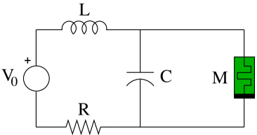
Figure 1: Murali-Lakshmanan-Chua circuit.

We illustrate the form of this polynomial in terms of the example depicted in Figure 1, taken from [16]. Specifically, our purpose is to detail in an example how the different coefficients in the multihomogeneous characteristic polynomial (29) can be examined in terms of the spanning-tree structure of the circuit, and show the way in which eventual restrictions in the controlling variables are captured via dehomogenization. First, it is easy to check that only spanning trees including the voltage source define nonzero products in (29): the attention will be henceforth restricted to trees including the voltage source without further explicit mention. Additionally, the absence of loops defined exclusively by voltage sources and capacitors, and of cutsets just defined by current sources (absent in this example) and inductors, guarantees that, generically, the order of the circuit (that is, the degree of the characteristic polynomial) equals the number of memristors and reactive elements (see [30]). Actually, the leading term of the characteristic polynomial is defined by the set of spanning trees including the capacitor and excluding the inductor. There is only one such tree, depicted on the left of Figure 2. Since the resistor is in the tree but the memristor is not, this yields a leading coefficient of the form

$$LCP_{r}Q_{m}\lambda^{3}.$$

According to (29) the coefficient of $\lambda^{2}$ is defined in this case by the spanning trees which include either both or none of the reactive elements. These are the remaining trees in Figure 2, and yield the term

$$(CQ_{r}Q_{m}+LP_{r}P_{m})\lambda^{2}.$$

Finally, the coefficient of $\lambda$ is defined by the trees which include the inductor but not the capacitor. These are displayed in Figure 3. The corresponding term is

$$(P_{r}Q_{m}+P_{m}Q_{r})\lambda$$

and the full characteristic polynomial reads as

$$LCP_{r}Q_{m}\lambda^{3}+(CQ_{r}Q_{m}+LP_{r}P_{m})\lambda^{2}+(P_{r}Q_{m}+P_{m}Q_{r})\lambda.$$ (30)

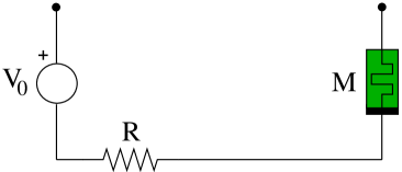
Figure 2: Spanning trees yielding the $\lambda^{3}$ and $\lambda^{2}$ terms.

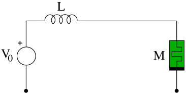
Figure 3: Spanning trees defining the term in $\lambda$.

We emphasize the fact that our approach applies without the need to assume neither a specific voltage- or current-controlled form for resistors nor a flux- or charge-controlled description of memristors; this means that (30) holds without any such restrictions. Again, particular forms can be obtained by dehomogenization under specific hypotheses: for example, in [16] the authors assume that the resistor is linear and current-controlled and that the memristor is flux-controlled. This case is obtained by dividing (30) by $P_{r}$ and $Q_{m}$ to get the resistance $R$ as the quotient $Q_{r}/P_{r}$ and the memductance $W$ as $P_{m}/Q_{m}$. This transforms (30) into

$$LC\lambda^{3}+(RC+LW)\lambda^{2}+(1+RW)\lambda,$$ (31)

an expression which is obtained (with normalized parameters) in [16] only after linearizing a state-space model of the circuit. Even if such assumptions are reasonable in many practical cases, notice that some key information is lost when turning from (30) to (31). In particular, (31) provides no information about the dual setting to the one considered in [16]. Indeed, should the resistor be voltage-controlled (and described by the conductance $G$) and/or the memristor charge-controlled (with memristance $M$), singularities due to the eventual vanishing of $G$ or $M$ would not be captured in (31). This means that there is no chance to describe such singularities (and the corresponding order reduction, possibly responsible for impasse phenomena: see [9] in this regard) by looking at (31). By contrast, the general form depicted in (30) captures these cases in a smooth manner simply by fixing respectively the parameter values $P_{r}=0$ or $Q_{m}=0$, both of which annihilate the leading term of (30).

4 Simple stationary bifurcation points in nonlinear circuits

The formalism introduced in previous sections provides a set of useful tools for qualitative studies of the dynamics of nonlinear circuits. In particular, in what follows we apply our framework to a bifurcation analysis, focusing on steady bifurcations of dynamic circuits without memristors. The goal is to provide a characterization of so-called simple stationary bifurcation points in graph-theoretic terms, that is, a characterization explicitly formulated in terms of certain assumptions on the topology of the circuit and the electrical properties of the devices. This extends previous studies of other bifurcations in the circuit context [11, 31].

4.1 Stationary bifurcations

Consider an explicit ODE $x^{\prime}=F(x,\mu)$, $x\in\Omega\subseteq\mathbb{R}^{n}$, and let the origin (assumed to belong to $\Omega$) be an equilibrium for any $\mu$ on a neighborhood of a given $\mu_{0}$. In this setting, the point $(0,\mu_{0})$ is called a simple stationary bifurcation point if the following conditions hold:

• $\lambda=0$ is a simple eigenvalue of $F_{x}(0,\mu_{0})$; and

• $F_{x\mu}(0,\mu_{0})v\notin\mathrm{im}\hskip 1.42262ptF_{x}(0,\mu_{0})$ for $v\in\mathrm{ker}\hskip 1.42262ptF_{x}(0,\mu_{0})-\{0\}$.

Here we are using the subscripts $x$ and $\mu$ to denote partial differentiation. Find detailed introductions to stationary bifurcations in [26, 33]: note only that the conditions above can be stated in this straightforward form because of the assumption that the origin is, at least locally, an equilibrium for any $\mu$. For our present purposes, the important remark is that under additional requirements (namely, a second order transversality condition and the absence of other eigenvalues in the imaginary axis), a simple stationary bifurcation point as defined above is well-known to be responsible for a transcritical bifurcation [26], displaying an exchange of stability between two equilibrium branches; this will be the case in the example considered at the end of this section.

4.2 A circuit-theoretic characterization of the bifurcation

Theorem 5 below presents a graph-theoretic characterization of the existence of simple stationary bifurcation points in nonlinear circuits, in the presence of certain topological configurations. The bifurcation phenomenon will be related to a distinguished resistor (supposed w.l.o.g. to be the first one), which is here assumed to be voltage-controlled, with a characteristic of the form

$$i=g(v,\mu)=\mu v+\tilde{g}(v),$$ (32)

with $\tilde{g}(v)=o(|v|)$. Note that $\mu$ is the incremental conductance at the origin and our purpose is to characterize the bifurcation conditions with this conductance behaving as the bifurcation parameter. Because of the form of (32) we have $g(0,\mu)=0$. The remaining resistors are assumed to be characterized by arbitrary submersions $f_{j}(i_{j},v_{j}).$

In the statement of Theorem 5 we split the hypotheses into those referring to the circuit topology (hypotheses T1 and T2) and the ones involving the electrical properties of the constitutive devices (D1, D2 and D3). We will make use of the notion of a proper tree, which is a spanning tree including all capacitors and no inductors. We denote the family of proper trees by ${\cal T}_{p}$.

Theorem 5.

Consider an uncoupled electrical circuit for which the following hypotheses hold:

1. There are no loops or cutsets defined by only one type of reactive elements (capacitors or inductors).

2. The bifurcating resistor (governed by (32)) forms a cutset together with one or more capacitors.

3. The characteristics of all resistors meet the origin.

4. All circuit devices but the bifurcating resistor are strictly locally passive at the origin.

5. The sum $\displaystyle\sum_{T\in{\cal T}_{p}}\left(\hskip 1.42262pt\prod_{j\in T_{r}}\frac{\partial f_{j}}{\partial v_{j}}(0,0)\prod_{k\in\overline{T}_{k}}\frac{\partial f_{k}}{\partial i_{k}}(0,0)\right),$ ranging over proper trees, does not vanish.

Then $\mu_{0}=0$ yields a simple stationary bifurcation point at the origin.

Proof. Note first that because of the condition $g(0,\mu)=0$ holding for the bifurcating resistor (cf. (32)), together with hypothesis D1, the origin happens to be an equilibrium for any value of the parameter $\mu$. We therefore need to check that conditions (i) and (ii) in subsection 4.1 hold, in the understanding that the vector field $F$ arising there comes from the reduction of the differential-algebraic model (14), in the terms detailed later.

Let us first focus on condition (i), which in our context amounts to saying that the characteristic polynomial (17) has a null independent term at the origin (so that $\lambda=0$ is an eigenvalue) with the coefficient of the term in $\lambda$ not vanishing (this making $\lambda=0$ a simple eigenvalue). To check this we have to examine the form of such coefficients in light of the hypotheses above.

The independent term in (17) is given by the sum

$$\sum_{T\in{\cal T}_{p}^{*}}\prod_{j\in T_{r}}\frac{\partial f_{j}}{\partial v_{j}}(0,0)\prod_{k\in\overline{T}_{k}}\left(-\frac{\partial f_{k}}{\partial i_{k}}(0,0)\right),$$ (33)

ranging over spanning trees which include all inductors and no capacitors (we denote the family of such trees by ${\cal T}_{p}^{*}$). At least one such tree exists because of the absence of inductor loops and capacitor cutsets assumed in T1. The key fact at this point is that all trees in ${\cal T}_{p}^{*}$ have the bifurcating resistor as a twig. This is a consequence of an elementary graph-theoretic property, namely, that a spanning tree must include at least one branch from every cutset; since capacitors are necessarily excluded from the spanning trees in ${\cal T}_{p}^{*}$, hypothesis T2 implies that the bifurcating resistor enters all such trees. Now, by setting $f_{1}=-i_{1}+\mu v_{1}+\tilde{g}(v_{1})$ for the bifurcating resistor (cf. (32)), we have $\partial f_{1}/\partial v_{1}=\mu$ at the origin, so that $\mu$ is a common factor to all the summands in (33). Additionally, by the strict passivity assumption stated in hypothesis D2, all summands in (33) must display the same sign, regardless of the actual choice of the defining submersions. Indeed, the passivity condition implies that $\partial f_{j}/\partial v_{j}$ and $-\partial f_{j}/\partial i_{j}$ have at the origin the same sign for each $j$ (exception made of $j=1$, that is, of the bifurcating resistor), and the claim then follows easily from the multihomogeneous form of the polynomial (10). This means that the independent term of the characteristic polynomial simply reads as $\mu k$ for some non-null constant $k$. In particular, this independent term vanishes at the bifurcation value $\mu=0$.

Regarding the term in $\lambda$ within the characteristic polynomial (17), notice that this term comes from all spanning trees which include either exactly one capacitor and all inductors in the tree, or exactly one inductor and all capacitors in the cotree. Again, one can check that at least one of such spanning trees does exist, since the replacement of the bifurcating resistor in any of the spanning trees in the paragraph above (namely, the ones defining the independent term of the characteristic polynomial) by one capacitor from the cutset defined in hypotheses T2 results in a spanning tree which includes exactly one capacitor and all inductors. The contribution of this term to the coefficient is non-zero because of the absence of the bifurcating resistor from the tree (so that it contributes a factor $-\partial f_{1}/\partial i_{1}=1$, with $f_{1}$ defined above) together with the assumption that all remaining devices are strictly locally passive. Since other spanning trees contribute to the sum terms which are zero (if such trees include the bifurcating resistor) or, as in the preceding paragraph, have otherwise the same sign as the one above (if they do not), one concludes that the coefficient of the term in $\lambda$ is non-null and this means that the zero eigenvalue is indeed a simple one.

It remains to check condition (ii) from subsection 4.1, that is, $F_{x\mu}v\notin\mathrm{im}\hskip 1.42262ptF_{x}$ for $v\in\mathrm{ker}\hskip 1.42262ptF_{x}-\{0\}$ (with all derivatives evaluated at the origin). From well-known properties of matrix analysis (see [15] or, specifically, Lemma 1 in [31]), this condition can be equivalently assessed as

$$\frac{\partial\det F_{x}}{\partial\mu}(0,\mu_{0})\neq 0.$$ (34)

In our setting $F$ stands for the vector field defining an explicit local reduction of the differential-algebraic model (14) at equilibrium: here we use hypothesis D3, which guarantees that the leading coefficient of the characteristic polynomial (17) does not vanish; worth remarking is that the capacitances and inductances are positive at the origin because of the strict local passivity hypothesis D2. This means that the matrix pencil (15) has nilpotency index one (cf. [2, 20]) and a state reduction of (14) (or, in other words, the vector field $F$ above) is thus well-defined in terms of $v_{c}$ and $i_{l}$ [29].

For our purposes there is no need to compute explicitly this reduced vector field; it is enough to use the Jacobian matrix $F_{x}$ at the origin, which by construction is the Schur reduction [15] $M_{1}/M_{2}$, with

$$M_{1}=\begin{pmatrix}0&0&(C(0))^{-1}&0&0&0\\ 0&0&0&(L(0))^{-1}&0&0\\ 0&A_{l}&A_{c}&0&A_{r}&0\\ B_{c}&0&0&B_{l}&0&B_{r}\\ 0&0&0&0&-Q&P\end{pmatrix}$$

coming from the linearization of (14), and

$$M_{2}=\begin{pmatrix}A_{c}&0&A_{r}&0\\ 0&B_{l}&0&B_{r}\\ 0&0&-Q&P\end{pmatrix}.$$

In both matrices we denote $P=\partial f_{r}/\partial v_{r}$, $Q=-\partial f_{r}/\partial i_{r}$, with the derivatives being always evaluated at equilibrium. We leave it to the reader to check that $M_{2}$ is non-singular because of hypothesis D3. Now, a well-known property of the Schur reduction says that

$$\det M_{1}=\det M_{2}\det F_{x}.$$ (35)

Additionally, since as shown above the matrix pencil (and hence the linearized vector field $F_{x}$) has a zero eigenvalue at equilibrium, we have $\det F_{x}=0$ at the origin and, by differentiating (35) we may hence evaluate (34) as

$$\frac{\partial\det M_{1}}{\partial\mu}\neq 0.$$ (36)

However, up to a non-zero factor the determinant of $M_{1}$ equals

$$\det\begin{pmatrix}A_{c}&A_{l}&A_{r}&0&0&0\\ 0&0&0&B_{c}&B_{l}&B_{r}\\ I_{c}&0&0&0&0&0\\ 0&0&0&0&I_{l}&0\\ 0&0&-Q&0&0&P\end{pmatrix}.$$ (37)

Using Theorem 2 one can check that the latter determinant is given by the sum (33) (because tree capacitors or cotree inductors yield a null factor in the corresponding term, in light of the form of the matrix in (37)), again possibly up to a sign. As shown in the first part of the proof, this sum is given by $\mu k$ for some non-vanishing constant $k$. This means that the derivative in (36) is not zero, as we aimed to show. From (36) it follows that (34) is met: therefore, condition (ii) also holds and the proof is complete. $\Box$

4.3 Example

Finally, we illustrate the result stated in Theorem 5 by means of an elementary example, depicted in Figure 4. This circuit may also help the reader understand the expression (17) derived for the characteristic polynomial in subsection 3.3.

Figure 4: A circuit undergoing a transcritical bifurcation.

The resistor labelled as $R_{1}$ will behave as the bifurcating device, and is therefore assumed to be governed by an expression of the form depicted in (32), that is,

$$i_{1}=g_{1}(v_{1},\mu)=\mu v_{1}+\tilde{g}(v_{1}).$$

Note that it forms a cutset together with the capacitor, since the removal of both branches disconnects the circuit. The key topological hypothesis in Theorem 5 (hypothesis T2) is therefore met. For simplicity, we take $\tilde{g}(v_{1})=v_{1}^{2}$. For later use, let additionally $f_{1}(i_{1},v_{1},\mu)$ stand for $i_{1}-g_{1}(v_{1},\mu)$. The capacitor and the inductor are assumed to be linear and strictly passive, with positive capacitance and inductance $C$ and $L$, respectively. Finally, we give the second resistor an implicit form, that is, we write its characteristic in the form $f_{2}(i_{2},v_{2})=0$, and assume $f_{2}(0,0)=0$.

Defining directions by choosing top-down orientations in the branches depicted in vertical in the figure, the circuit equations can be easily written as follows:

$$Cv_{c}^{\prime} = g_{1}(v_{1},\mu)$$ (38a)

$$Li_{l}^{\prime} = v_{1}+v_{c}$$ (38b)

$$0 = i_{l}+i_{2}+g_{1}(v_{1},\mu)$$ (38c)

$$0 = f_{2}(i_{2},v_{1}+v_{c}),$$ (38d)

where we have performed some elementary simplifications with respect to the general model (14) (in particular, the voltage across the inductor and the second resistor is written in terms of $v_{1}$ and $v_{c}$ in (38b) and (38d)).

In this setting, the circuit can be easily checked to have two equilibrium loci, defined by $v_{1}=0$ and $v_{1}=-\mu$ (together with $v_{c}=-v_{1},$ $i_{l}=i_{2}=0$), which intersect at the origin. For the sake of simplicity in the notation, we introduce the parameters

$$P_{j}=\frac{\partial f_{j}}{\partial v_{j}},\ Q_{j}=-\frac{\partial f_{j}}{\partial i_{j}},\ j=1,2,$$

with $f_{1}$ and $f_{2}$ defined above. The multihomogeneous form (17) of the characteristic polynomial reads at equilibrium as

$$LC(P_{1}Q_{2}+Q_{1}P_{2})\lambda^{2}+(CQ_{1}Q_{2}+LP_{1}P_{2})\lambda+P_{1}Q_{2},$$ (39)

an expression that the reader may derive either from linearizing (38) or by examining the structure of the spanning trees of the circuit, as we did in subsection 3.4.3.

To illustrate more easily the notions used in Theorem 5, let us restrict the attention to cases in which both resistors admit a voltage-controlled description. This is equivalent to dehomogenize the polynomial above by dividing by $Q_{1}Q_{2}$, to get

$$LC(G_{1}+G_{2})\lambda^{2}+(C+LG_{1}G_{2})\lambda+G_{1}.$$ (40)

The non-vanishing of the leading coefficient amounts to the condition $LC(G_{1}+G_{2})\neq 0$: both $L$ and $C$ are non-zero (actually positive) by hypothesis, whereas the non-vanishing condition on $G_{1}+G_{2}$ reflects in this case the general requirement expressed by hypothesis D3 in Theorem 5. Note in this direction that the circuit has two proper trees, defined by the capacitor and each one of the two resistors, which are responsible for the $G_{1}+G_{2}$ expression above (or, in greater generality, for the term $P_{1}Q_{2}+Q_{1}P_{2}$ in the multihomogeneous expression (39)). Focusing the attention on the bifurcation value $\mu=0$, we have $G_{1}=0$ at the origin, and the requirement $G_{1}+G_{2}\neq 0$ is in this case actually met by the strict passivity assumption on the second resistor (which means that $G_{2}>0$). The reader may check that all the remaining hypotheses of Theorem 5 are met and, therefore, a simple stationary bifurcation point is expected to be displayed at the origin. This is actually the case and, moreover, a transcritical bifurcation occurs at that point: indeed, the system experiences an exchange of stability, since the equilibrium branch defined by $v_{1}=0$ can be checked to be asymptotically stable for $\mu>0$ but unstable for $\mu<0$, whereas the opposite holds for the branch $v_{1}=-\mu$.

5 Concluding remarks

Because of their generality, we believe the results of Section 2, involving the description of smooth planar curves as equivalence classes of submersions, to be of potential interest in different branches of applied mathematics. In the context of nonlinear circuit theory, this formalism has led to a framework where homogeneous forms for incremental magnitudes can be handled systematically, making it easier to analyze different properties of circuits with implicit characteristics, both in the classical and in the memristive context. Such analyses admit several extensions: let us mention, in particular, that all the results concerning dynamic circuits can be easily extended to accommodate implicit characteristics in reactive devices, and that most ideas seem to be applicable to circuits with memcapacitors and meminductors. Distributed systems can be possibly included in the same formalism. Our approach should be useful in other qualitative studies: in the scope of future research is the formulation of Routh-Hurwitz criteria for electrical circuits in graph-theoretic terms, using the general multihomogeneous description of the characteristic polynomial here discussed. This should be of help in a general analysis of stability problems in nonlinear circuits. The study of other bifurcations, including bifurcations without parameters in memristive circuits, may also benefit from our approach.

References

- [1] B. Bollobás, Modern Graph Theory, Springer-Verlag, 1998.
- [2] K. E. Brenan, S. L. Campbell and L. R. Petzold, Numerical Solution of Initial-Value Problems in Differential-Algebraic Equations, SIAM, 1996.
- [3] P. R. Bryant, The order of complexity of electrical networks, Proceedings of the IEE, Part C 106 (1959) 174-188.
- [4] R. E. Bryant, J. D. Tygar and L. P. Huang, Geometric characterization of series-parallel variable resistor networks, IEEE Trans. Circuits Syst. I 41 (1994) 686-698.
- [5] S. Chaiken, Ported Tutte functions of extensors and oriented matroids, ArXiv, 2006.
- [6] S. Chaiken and D. J. Kleitman, Matrix tree theorems, J. Combinatorial Theory A 24 (1978) 377-381.
- [7] W.-K. Chen, Graph Theory and its Engineering Applications, World Scientific, 1997.
- [8] L. O. Chua, Memristor – The missing circuit element, IEEE Trans. Circuit Theory 18 (1971) 507-519.
- [9] F. Corinto and M. Forti, Memristor circuits: Flux-charge analysis method, IEEE Trans. Circuits Syst. I 63 (2016) 1997-2009.
- [10] M. Di Ventra, Y. V. Pershin and L. O. Chua, Circuit elements with memory: memristors, memcapacitors and meminductors, Proc. IEEE 97 (2009) 1717-1724.
- [11] I. García de la Vega and R. Riaza, Saddle-node bifurcations in classical and memristive circuits, Internat. J. Bifur. Chaos 26 (2016) 1650064.
- [12] M. Giaquinta and G. Modica, Mathematical Analysis, Birkhäuser, 2009.
- [13] F. M. Hall, An Introduction to Abstract Algebra, Cambridge University Press, 1972.
- [14] R. Hartshorne, Algebraic Geometry, Springer, 1977.
- [15] R. A. Horn and Ch. R. Johnson, Matrix Analysis, Cambridge Univ. Press, 1985.
- [16] A. Ishaq Ahamed and M. Lakshmanan, Discontinuity induced Hopf and Neimark–Sacker bifurcations in a memristive Murali-Lakshmanan-Chua circuit, Internat. J. Bifur. Chaos 27 (2017), 1730021.
- [17] M. Itoh and L. O. Chua, Memristor oscillators, Internat. J. Bifur. Chaos 18 (2008) 3183-3206.
- [18] M. Itoh and L. O. Chua, Parasitic effects on memristor dynamics, Internat. J. Bifur. Chaos 26 (2016) 1630014.
- [19] P. Kunkel and V. Mehrmann, Differential-Algebraic Equations. Analysis and Numerical Solution, EMS, 2006.
- [20] R. Lamour, R. März and C. Tischendorf, Differential-Algebraic Equations. A Projector Based Analysis, Springer, 2013.
- [21] J. M. Lee, Introduction to Smooth Manifolds, Springer, 2013.
- [22] M. Messias, C. Nespoli and V. A. Botta, Hopf bifurcation from lines of equilibria without parameters in memristors oscillators, Internat. J. Bifur. Chaos 20 (2010) 437-450.
- [23] B. Muthuswamy, Implementing memristor based chaotic circuits, Internat. J. Bifur. Chaos 20 (2010) 1335-1350.
- [24] B. Muthuswamy and L. O. Chua, Simplest chaotic circuit, Internat. J. Bifur. Chaos 20 (2010) 1567-1580.
- [25] A. Penin, Analysis of Electrical Circuits with Variable Load Regime Parameters, Springer, 2015.
- [26] L. Perko, Differential Equations and Dynamical Systems, Springer, 2001.
- [27] P. J. Rabier and W. C. Rheinboldt, Nonholonomic Motion of Rigid Mechanical Systems from a DAE Viewpoint, SIAM, 2000.
- [28] P. J. Rabier and W. C. Rheinboldt, Theoretical and numerical analysis of differential-algebraic equations, in P. G. Ciarlet et al. (eds.), Handbook of Numerical Analysis, Vol. VIII, pp. 183-540, North Holland/Else vier, 2002.
- [29] R. Riaza, Differential-Algebraic Systems, World Scientific, 2008.
- [30] R. Riaza, Nondegeneracy conditions for active memristive circuits, IEEE TransĊircuits Syst. II 57 (2010) 223-227.
- [31] R. Riaza, Transcritical bifurcation without parameters in memristive circuits, SIAM J. Appl. Math. 78 (2018) 395-417.
- [32] R. Riaza, Circuit theory in projective space and homogeneous circuit models, IEEE Trans. Circuits Syst. I 66 (2019) 463-476.
- [33] R. Seydel, Practical Bifurcation and Stability Analysis, Springer, 2010.
- [34] C. A. B. Smith, Electric currents in regular matroids, in D. Welsh and D. Woodall (eds.), Combinatorics, pp. 262-284, IMA, 1972.
- [35] M. Spivak, Calculus on Manifolds, Addison-Wesley, 1965.
- [36] D. B. Strukov, G. Snider, D. Stewart and R. S. Williams, The missing memristor found, Nature 453 (2008) 80-83.
- [37] R. Tetzlaff (ed.), Memristors and Memristive Systems, Springer, 2014.
- [38] L. W. Tu, An Introduction to Manifolds, Springer, 2011.
- [39] S. Vaidyanathan and C. Bolos, Advances in Memristors, Memristive Devices and Systems, Springer, 2017.