A Sturm–Liouville theorem for quadratic operator pencils

Abstract

We establish a Sturm–Liouville theorem for quadratic operator pencils counting their unstable real roots, with applications to stability of waves. Such pencils arise, for example, in reduction of eigenvalue systems to higher-order scalar problems.

1 Introduction

In this paper, motivated by recent results of [26] in a special case, we establish a general Sturm–Liouville problem for quadratic operator pencils on the half- or whole-line. Specifically, we consider eigenvalue problems on the half line,

$$\begin{split}&y^{\prime\prime}+V(x)y=\lambda f_{1}(x)y+\lambda^{2}f_{2}(x)y;\quad x\in{\mathbb{R}}_{-},\\ &(c+\phi(\lambda))y(0)-y^{\prime}(0)=0.\end{split}$$ (1.1)

and on the whole line,

$$y^{\prime\prime}+V(x)y=\lambda f_{1}(x)y+\lambda^{2}f_{2}(x)y;\quad x\in{\mathbb{R}},$$ (1.2)

where $\phi$ is a complex analytic matrix-valued function. The matrix $c\in M_{n}(\mathbb{C})$ is Hermitian and $\phi(\lambda)$ is Hermitian for $\lambda\in\mathbb{R}$, $V,f_{j}\in C(\mathbb{R},\mathbb{C}^{n\times n})$ are Hermitian potentials. We also list the following assumptions:

(A1) The limits $\lim_{x\to-\infty}V(x)=V_{-}$ and $\lim_{x\to-\infty}f_{j}(x)=f_{j-}$ exist, and $V-V_{-},f_{j}-f_{j-}\in L^{1}({\mathbb{R}})$, $f_{1}>0$ and $f_{2}\geq\delta>0$, and there is $\gamma<0$ such that, for all $\mu\in{\mathbb{R}}$ and all $\lambda\in{\mathbb{C}}$,

$$\det(-\mu^{2}+V_{-}-\lambda f_{1-}-\lambda^{2}f_{2-})=0$$ (1.3)

implies

$$\Re\lambda\leq\gamma<0.$$ (1.4)

(A2) $\phi(0)=0$ and $\phi^{\prime}(\lambda)<0$ for $\lambda\in\mathbb{R}_{+}$.

(A3) ${\text{\rm sign }}\Im\lambda\Im\phi(\lambda)\leq 0$ for all $\lambda$ with $\Re\lambda\geq 0$.

(A4) The limits $\lim_{x\to\pm\infty}V(x)=V_{\pm}$ and $\lim_{x\to\pm\infty}f_{j}(x)=f_{j\pm}$ exist, and $V-V_{\pm},f_{j}-f_{j\pm}\in L^{1}({\mathbb{R}})$, $f_{1}>0$ and $f_{2}\geq\delta>0$, and there is $\gamma<0$ such that, for all $\mu\in{\mathbb{R}}$ and all $\lambda\in{\mathbb{C}}$,

$$\det(-\mu^{2}+V_{\pm}-\lambda f_{1\pm}-\lambda^{2}f_{2\pm})=0$$ (1.5)

implies

$$\Re\lambda\leq\gamma<0.$$ (1.6)

(A4) is related to problem (1.2); (A1), (A2) and (A3) are related to problem (1.1). Our particular interest lies in counting the number of real nonnegative eigenvalues of (1.2) and (1.1). As described further in Section 6, quadratic eigenvalue problems (1.2)–(1.1) arise for example through reduction of a standard eigenvalue system to a higher-order system in a lower-dimensional variable. As such, their stability has bearing on stability of traveling waves, calculus of variations, etc. In particular, reduction of a first-order $2\times 2$ system to a second-order scalar problem can always be performed [13, 26, 28], in which case the assumptions of Hermitian coefficients, since they are real scalar, is automatically satisfied.

We consider at the same time the truncated eigenvalue problems

$$\begin{split}&y^{\prime\prime}+V(x)y=\lambda f_{1}(x)y+\lambda^{2}f_{2}(x)y;\quad x\in{\mathbb{R}}_{L}:=(-\infty,L],\,\,L\in\mathbb{R},\\ &y(L)=0.\end{split}$$ (1.7)

Next, we introduce the corresponding operator pencils:

$$\begin{split}&\mathcal{L_{-}}(\lambda):\operatorname{dom}(\mathcal{L}_{-}(\lambda))\subset(L^{2}({\mathbb{R}}_{-}))^{n}\to(L^{2}({\mathbb{R}}_{-}))^{n},\\ &\mathcal{L_{-}}(\lambda)y:=y^{\prime\prime}+V(x)y-\lambda f_{1}(x)y-\lambda^{2}f_{2}(x)y,\,y\in\operatorname{dom}(\mathcal{L}_{-}(\lambda)),\quad x\in{\mathbb{R}}_{-},\\ &\operatorname{dom}(\mathcal{L}_{-}(\lambda))=\{y\in(H^{2}({\mathbb{R}}_{-}))^{n}:(c+\phi(\lambda))y(0)-y^{\prime}(0)=0\}.\end{split}$$ (1.8)

And

$$\begin{split}&\mathcal{L}_{L}(\lambda):\operatorname{dom}(\mathcal{L}_{L}(\lambda))\subset(L^{2}({\mathbb{R}}_{L}))^{n}\to(L^{2}({\mathbb{R}}_{L}))^{n},\\ &\mathcal{L}_{L}(\lambda)y:=y^{\prime\prime}+V(x)y-\lambda f_{1}(x)y-\lambda^{2}f_{2}(x)y,\,y\in\operatorname{dom}(\mathcal{L}_{L}(\lambda)),\quad x\in{\mathbb{R}}_{L},\\ &\operatorname{dom}(\mathcal{L}_{L}(\lambda))=\{y\in(H^{2}({\mathbb{R}}_{L}))^{n}:y(L)=0\}.\end{split}$$ (1.9)

Finally,

$$\begin{split}&\mathcal{L}(\lambda):\operatorname{dom}(\mathcal{L}(\lambda))\subset(L^{2}({\mathbb{R}}))^{n}\to(L^{2}({\mathbb{R}}))^{n},\\ &\mathcal{L}(\lambda)y:=y^{\prime\prime}+V(x)y-\lambda f_{1}(x)y-\lambda^{2}f_{2}(x)y,\,y\in\operatorname{dom}(\mathcal{L}(\lambda)),\quad x\in{\mathbb{R}},\\ &\operatorname{dom}(\mathcal{L}(\lambda))=(H^{2}({\mathbb{R}}))^{n}.\end{split}$$ (1.10)

Essential spectrum. Our first goal is to show that Assumption (A1) implies that there exists an open subset $\Omega$ containing the closed right half plane that consists of either points of the resolvent set or isolated eigenvalues of finite algebraic multiplicity of the operator pencil $\mathcal{L_{-}}(\cdot)$.

We introduce the closed densely defined operator pencil $\mathcal{T}(\lambda):\mathcal{D(\lambda)}\to\mathcal{H}$, where $\mathcal{D(\lambda)}\subset\mathcal{H}$ is the domain of $\mathcal{T}(\lambda)$.

Definition 1.1.

(essential spectrum) The essential spectrum of $\mathcal{T}$, denoted $\sigma_{ess}(\mathcal{T})$, is the set of all complex numbers $\lambda$ such that $\mathcal{T}(\lambda)$ is not a Fredholm operator with index $0$.

Since for the half-line case, the domain of the operator pencil is $\lambda$ dependent, we couldn’t find a precise reference for the following lemma which we prove in Appendix B.

Lemma 1.1.

Let Assumption (A1) hold. Then $\Omega\subset{\mathbb{C}}\setminus\sigma_{ess}(\mathcal{L_{-}})$. Moreover, $\Omega$ consists of either points of the resolvent set or isolated eigenvalues of finite algebraic multiplicity of the operator pencil $\mathcal{L_{-}}(\cdot)$.

Similarly,

Lemma 1.2.

Let Assumption (A4) hold. Then $\Omega\subset{\mathbb{C}}\setminus\sigma_{ess}(\mathcal{L}_{L})$. Moreover, $\Omega$ consists of either points of the resolvent set or isolated eigenvalues of finite algebraic multiplicity of the operator pencil $\mathcal{L}_{L}(\cdot)$.

For purpose of self-containment, we also provide the proof of the following lemma in Appendix B.

Lemma 1.3.

Let Assumption (A4) hold. Then $\Omega\subset{\mathbb{C}}\setminus\sigma_{ess}(\mathcal{L})$. Moreover, $\Omega$ consists of either points of the resolvent set or isolated eigenvalues of finite algebraic multiplicity of the operator pencil $\mathcal{L}(\cdot)$.

Maslov index. As a starting point, we define what we will mean by a Lagrangian subspace of $\mathbb{C}^{2n}$.

Definition 1.2.

We say $\ell\subset\mathbb{C}^{2n}$ is a Lagrangian subspace of $\mathbb{C}^{2n}$ if $\ell$ has dimension $n$ and

$$(J_{2n}u,v)_{\mathbb{C}^{2n}}=0,$$ (1.11)

for all $u,v\in\ell$. Here, $(\cdot,\cdot)_{\mathbb{C}^{2n}}$ denotes the standard inner product on $\mathbb{C}^{2n}$. In addition, we denote by $\Lambda(n)$ the collection of all Lagrangian subspaces of $\mathbb{C}^{2n}$, and we will refer to this as the Lagrangian Grassmannian.

Any Lagrangian subspace of $\mathbb{C}^{2n}$ can be spanned by a choice of $n$ linearly independent vectors in $\mathbb{C}^{2n}$. We will generally find it convenient to collect these $n$ vectors as the columns of a $2n\times n$ matrix $\mathbf{X}$, which we will refer to as a frame for $\ell$. Moreover, we will often coordinatize our frames as $\mathbf{X}={X\choose Y}$, where $X$ and $Y$ are $n\times n$ matrices.

Suppose $\ell_{1}(\cdot),\ell_{2}(\cdot)$ denote paths of Lagrangian subspaces $\ell_{i}:\mathcal{I}\to\Lambda(n)$, for some parameter interval $\mathcal{I}$. The Maslov index associated with these paths, which we will denote $\operatorname{Mas}(\ell_{1},\ell_{2};\mathcal{I})$, is a count of the number of times the paths $\ell_{1}(\cdot)$ and $\ell_{2}(\cdot)$ intersect, counted with both multiplicity and direction. (In this setting, if we let $t_{*}$ denote the point of intersection (often referred to as a conjugate point), then multiplicity corresponds with the dimension of the intersection $\ell_{1}(t_{*})\cap\ell_{2}(t_{*})$; a precise definition of what we mean in this context by direction will be given in Section 2.) In some cases, the Lagrangian subspaces will be defined along some path in the $(\alpha,\beta)$-plane

$$\Gamma=\{(\alpha(t),\beta(t)):t\in\mathcal{I}\},$$

and when it is convenient we will use the notation $\operatorname{Mas}(\ell_{1},\ell_{2};\Gamma)$.

We say that the evolution of $\mathcal{L}=(\ell_{1},\ell_{2})$ is monotonic provided all intersections occur with the same direction. If the intersections all correspond with the positive direction, then we can compute

$$\operatorname{Mas}(\ell_{1},\ell_{2};\mathcal{I})=\sum_{t\in\mathcal{I}}\dim(\ell_{1}(t)\cap\ell_{2}(t)).$$

Suppose $\mathbf{X}_{1}(t)={X_{1}(t)\choose Y_{1}(t)}$ and $\mathbf{X}_{2}(t)={X_{2}(t)\choose Y_{2}(t)}$ respectively denote frames for Lagrangian subspaces of $\mathbb{C}^{2n}$, $\ell_{1}(t)$ and $\ell_{2}(t)$. Then we can express this last relation as

$$\operatorname{Mas}(\ell_{1},\ell_{2};\mathcal{I})=\sum_{t\in\mathcal{I}}\dim\ker(\mathbf{X}_{1}(t)^{*}J\mathbf{X}_{2}(t)).$$

1.1 Main results

We establish the following generalized Sturm-Liouville theorems relating the spectral count, or number of real eigenvalues greater than a given nonnegative value $\lambda$, to the number of conjugate points of the Lagrangian frame asymptotic to the decaying eigenspace at $x\to-\infty$ plus, in the case of the half-line problem (1.1), a computable boundary correction term. Note that, in contrast to the standard case of a linear operator pencil, we do not obtain information for negative $\lambda$, but only about the number of possible unstable real eigenvalues $\lambda>0$. Nonetheless, this is sufficient to determine stability or instability of spectra, which is typically the question of interest.

Theorem 1.1.

For equation (1.1), let Assumptions (A1), (A2) hold, and let $\mathbf{X}$ and $\mathbf{X}_{\phi}$ denote the Lagrangian frames corresponding the unstable subpsace $E_{-}^{u}(x,\lambda)$ and the $\Phi(\lambda)$ subspace $\operatorname{colspan}{I_{n}\choose c+\phi(\lambda)}$, respectively. If $\mathcal{N}(\lambda)$ denotes the spectral count for (1.1) (the number of real eigenvalues that are greater than $\lambda$), then

$$\mathcal{N}(\lambda) =-\operatorname{Mas}(E_{-}^{u}(\cdot;\lambda),\Phi(\lambda);[-\infty,0])-\dim(\ker(\mathcal{L}_{-}(\lambda)))$$

$$+\operatorname{Mor}(\sqrt{\lambda f_{1-}+\lambda^{2}f_{2-}-V_{-}}-c-\phi(\lambda))+\dim\ker(\sqrt{\lambda f_{1-}+\lambda^{2}f_{2-}-V_{-}}-c-\phi(\lambda)),$$

$$\,\,\lambda\geq 0$$ .

Theorem 1.2.

For equation (1.7), let Assumption (A4) hold, and let $\mathbf{X}$ and $\mathbf{X}_{D}$ denote the Lagrangian frames corresponding to the unstable subpsace $E_{-}^{u}(x,\lambda)$ and the Dirichlet subspace $\mathcal{D}$, respectively. If $\mathcal{N}(\lambda)$ denotes the spectral count for (1.2) (the number of real eigenvalues that are greater than $\lambda$), then

$$\mathcal{N}(\lambda)=\sum_{-\infty<x<L}\dim(E_{-}^{u}(x,\lambda)\cap\mathcal{D})=\sum_{x\in(-\infty,L)}\dim\ker(\mathbf{X}(x;\lambda)^{*}J\mathbf{X}_{D}),\,\,\lambda\geq 0.$$

Theorem 1.3.

For equation (1.2), let Assumption (A4) hold, and let $\mathbf{X}$ and $\mathbf{X}_{D}$ denote the Lagrangian frames corresponding to the unstable subpsace $E_{-}^{u}(x,\lambda)$ and the Dirichlet subspace $\mathcal{D}$, respectively. If $\mathcal{N}(\lambda)$ denotes the spectral count for (1.2) (the number of real eigenvalues that are greater than $\lambda$), then

$$\mathcal{N}(\lambda)=\sum_{x\in{\mathbb{R}}}\dim(E_{-}^{u}(x,\lambda)\cap\mathcal{D})=\sum_{x\in{\mathbb{R}}}\dim\ker(\mathbf{X}(x;\lambda)^{*}J\mathbf{X}_{D}),\,\,\lambda\geq 0.$$

Typical examples of the eigenvalue curves

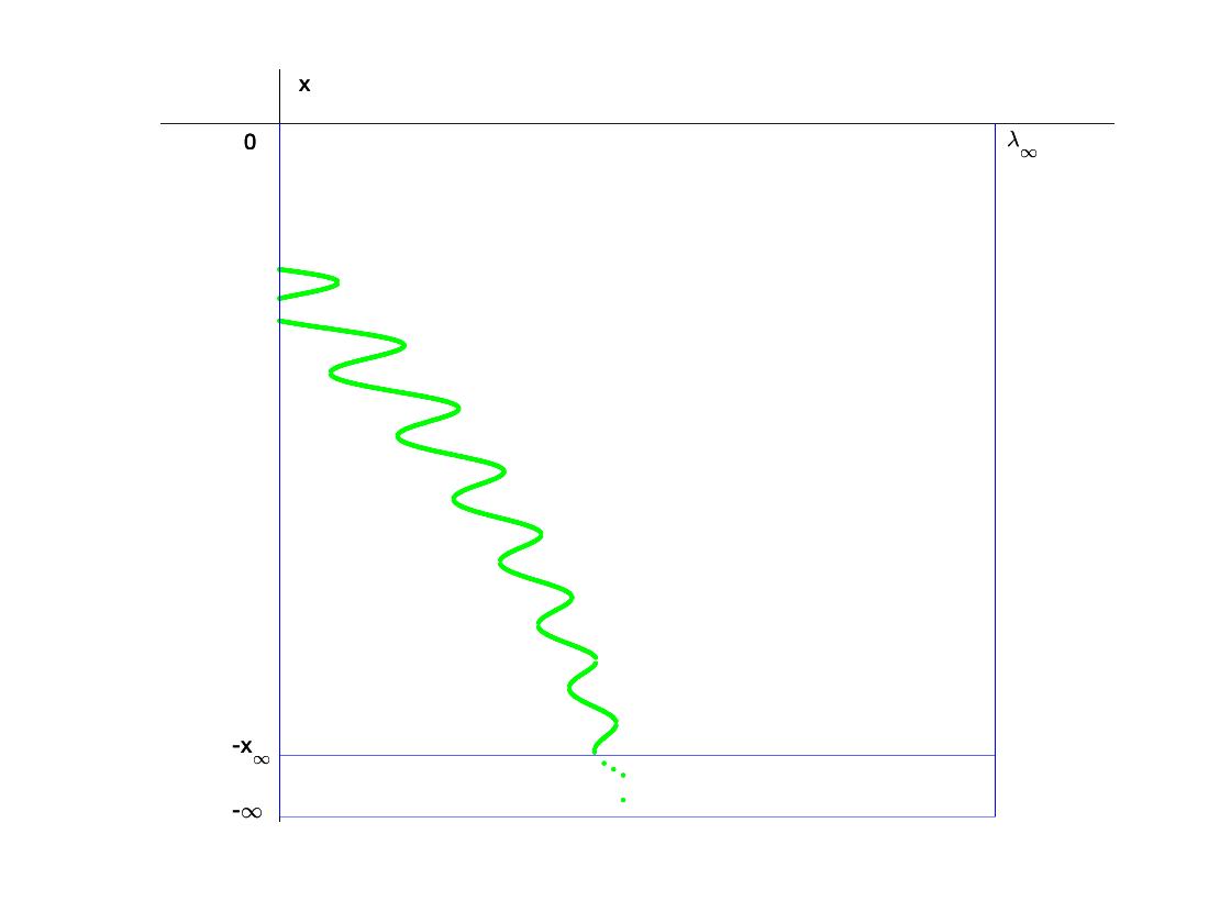
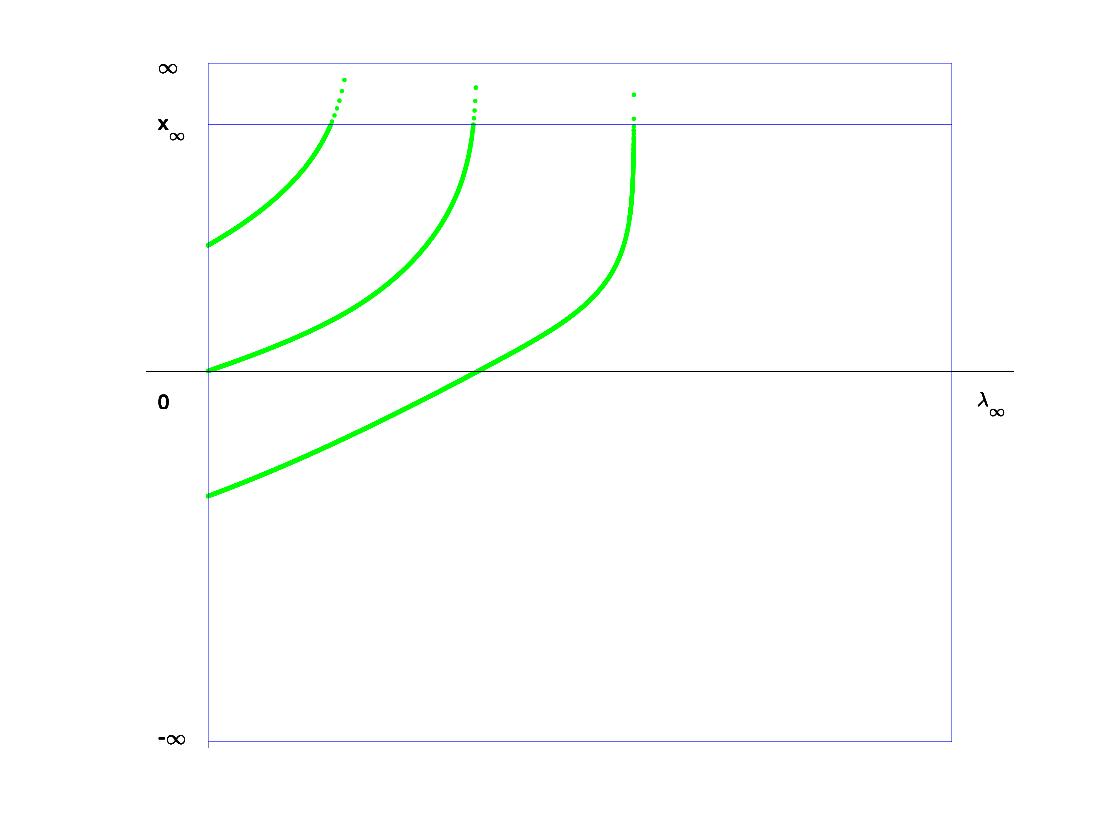
Figure 1: Eigenvalue curves

Example 1 (half-line, scalar) We consider the potentials
$V(x)=-1-(815+219\cos(1.8x))e^{0.1x}$, $f_{1}=1$, $f_{2}=2$ along with the boundary condition $(18-9\lambda)y(0)-y^{\prime}(0)=0$. In this case, we see the emergence of an eigenvalue from the bottom shelf, and we notice a very distinct loss of the monotonicity. See the left-half of Figure 1. The Maslov Index in this case is $1$, the Morse index of $\sqrt{-V_{-}}-c$ is $1$, and according to 1.1, this means that $\mathcal{N}(0)=0$ (the number of real eigenvalues for the problem (1.1) that are greater than $0$).

Example 2 (full-line, scalar) We consider the potentials $V(x)=-1+1.8e^{-0.06|x|}$, $f_{1}=1$, $f_{2}=2$. In this case, there can be no crossings along the bottom shelf, and indeed the only allowable behavior is for the eigenvalue curves to enter the box through the curve $\lambda=0$ and move upward until reaching the curve $x=\infty$. See the right-half of Figure 1. We ran our numerics up to some big positive value $x_{\infty}$. The number of intersections of the unstable subpsace $E_{-}^{u}(x,0)$ and the Dirichlet subspace $\mathcal{D}$ is 3, and according to Theorem 1.3 this means that $\mathcal{N}(0)=3$ (the number of real eigenvalues for the problem (1.2) that are greater than $0$).

Example 3 (half-line, $2\times 2$ system) We consider the potentials
$V(x)=\begin{pmatrix}-1-(815+219\cos(1.8x))e^{0.1x}&0\\ 0&-1-(255+0.1\cos(0.5x))e^{0.15x}\end{pmatrix}$, $f_{1}=I$ and $f_{2}=2I$ along with the boundary matrices $\phi(\lambda)=\begin{pmatrix}-9\lambda&0\\ 0&-9\lambda\end{pmatrix}$ and $c=\begin{pmatrix}18&2\\ 2&25\end{pmatrix}$. Note that the coupling appears via the matrix $c$. See the left-half of Figure 2. The Maslov Index in this case is $1$, the Morse index of $\sqrt{-V_{-}}-c$ is $2$, and according to 1.1, this means that $\mathcal{N}(0)=1$ (the number of real eigenvalues for the problem (1.1) that are greater than $0$).

Example 4 (full-line, $2\times 2$ system) We consider the potentials
$V(x)=\begin{pmatrix}-1+1.93e^{-0.141|x|}&0.5\\ 0.5&-1+1.93e^{-0.141|x|}\end{pmatrix}$, $f_{1}=I$ and $f_{2}=2I$. Note that the coupling appears via the potential $V$. See the right-half of Figure 2. The number of intersections of the unstable subpsace $E_{-}^{u}(x,0)$ and the Dirichlet subspace $\mathcal{D}$ is 5, and according to Theorem 1.3 this means that $\mathcal{N}(0)=5$ (the number of real eigenvalues for the problem (1.2) that are greater than $0$). Also, note that for the systems, the eigenvalue curves might intersect which can be observed for our particular $2\times 2$ system.

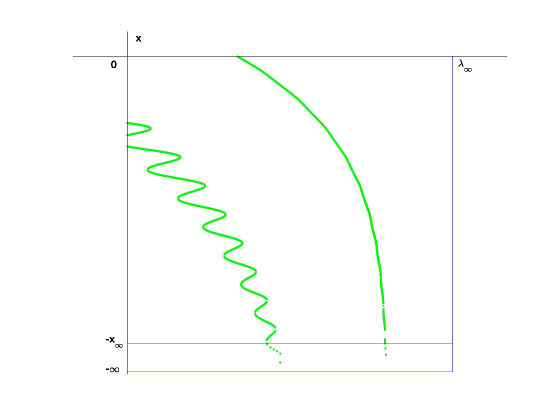
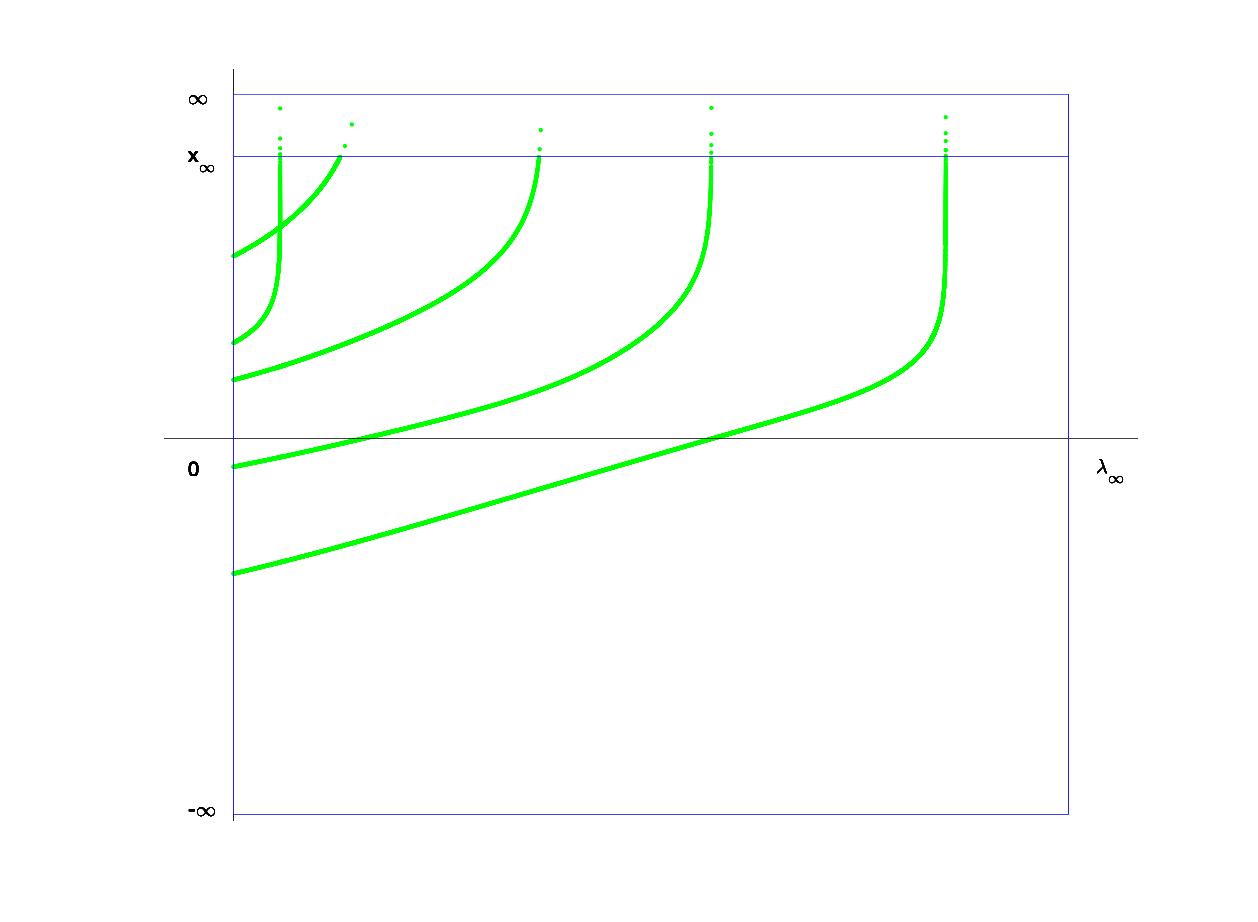
Figure 2: Eigenvalue curves

1.2 Reality of eigenvalues

The above theorems concern only the real spectrum of the associated operator pencil. However, adapting an argument of [26, Lemma 4.1] similar to that for the classic linear pencil case, we may readily see that nonstable spectra $\Re\lambda\geq 0$ of the whole-line problem are necessarily real, hence our conclusions are decisive for stability. Likewise, for the half-line problem, unstable spectra are real under the additional (sharp, see Remark 3.2) assumption that $\Im\phi(\lambda)\Im\lambda<0$ for $\Re\lambda\geq 0$; see Lemma 3.3.

2 The Maslov Index on $\mathbb{C}^{2n}$

Suppose $\mathbf{X}={X\choose Y}$, $\mathbf{X}_{D}={0\choose I_{n}}$ and $\mathbf{X}_{\phi}={I_{n}\choose c+\phi(\lambda)}$ respectively denote frames for Lagrangian subspaces $\ell(x,\lambda):=E_{-}^{u}(x,\lambda)$, the Dirichlet subspace $\mathcal{D}$ and the $\Phi(\lambda)$ subspace. We now set

$$\begin{split}\tilde{W}_{D}:&=(X+iY)(X-iY)^{-1},\\ \tilde{W}_{\phi}:&=-(X+iY)(X-iY)^{-1}(X_{\phi}-iY_{\phi})(X_{\phi}+iY_{\phi})^{-1},\\ \end{split}$$ (2.1)

noting that $\tilde{W}_{D}$ and $\tilde{W}_{\phi}$ detect intersections of $\ell=\operatorname{colspan}(\mathbf{X})=E_{-}^{u}(x,\lambda)$ with the Dirichlet subspace and the $\phi$ subspace, respectively. Moreover,

$$\begin{split}\dim\ker(\mathbf{X}^{*}J\mathbf{X}_{D})&=\dim\ker(\tilde{W}_{D}+I),\\ \dim\ker(\mathbf{X}^{*}J\mathbf{X}_{\phi})&=\dim\ker(\tilde{W}_{\phi}+I),\\ \end{split}$$

In general, given any two Lagrangian subspaces $\ell_{1}$ and $\ell_{2}$, with associated frames $\mathbf{X}_{1}={X_{1}\choose Y_{1}}$ and $\mathbf{X}_{2}={X_{2}\choose Y_{2}}$, we can define the complex $n\times n$ matrix

$$\tilde{W}=-(X_{1}+iY_{1})(X_{1}-iY_{1})^{-1}(X_{2}-iY_{2})(X_{2}+iY_{2})^{-1}.$$ (2.2)

Given two continuous maps $\ell_{1}(t),\ell_{2}(t)$ on a parameter interval $\mathcal{I}$, we denote by $\mathcal{L}(t)$ the path

$$\mathcal{L}(t)=(\ell_{1}(t),\ell_{2}(t)).$$

In what follows, we will define the Maslov index for the path $\mathcal{L}(t)$, which will be a count, including both multiplicity and direction, of the number of times the Lagrangian paths $\ell_{1}$ and $\ell_{2}$ intersect. In order to be clear about what we mean by multiplicity and direction, we observe that associated with any path $\mathcal{L}(t)$ we will have a path of unitary complex matrices as described in (2.2). We have already noted that the Lagrangian subspaces $\ell_{1}$ and $\ell_{2}$ intersect at a value $t_{*}\in\mathcal{I}$ if and only if $\tilde{W}(t_{*})$ has -1 as an eigenvalue. (Recall that we refer to the value $t_{*}$ as a conjugate point.) In the event of such an intersection, we define the multiplicity of the intersection to be the multiplicity of -1 as an eigenvalue of $\tilde{W}$ (since $\tilde{W}$ is unitary the algebraic and geometric multiplicites are the same). When we talk about the direction of an intersection, we mean the direction the eigenvalues of $\tilde{W}$ are moving (as $t$ varies) along the unit circle $S^{1}$ when they cross $-1$ (we take counterclockwise as the positive direction). We note that we will need to take care with what we mean by a crossing in the following sense: we must decide whether to increment the Maslov index upon arrival or upon departure. Indeed, there are several different approaches to defining the Maslov index (see, for example, [6, 23]), and they often disagree on this convention.

Following [5, 7, 22] (and in particular Definition 1.5 from [5]), we proceed by choosing a partition $a=t_{0}<t_{1}<\dots<t_{n}=b$ of $\mathcal{I}=[a,b]$, along with numbers $\epsilon_{j}\in(0,\pi)$ so that $\ker\big{(}\tilde{W}(t)-e^{i(\pi\pm\epsilon_{j})}I\big{)}=\{0\}$ for $t_{j-1}\leq t\leq t_{j}$; that is, $e^{i(\pi\pm\epsilon_{j})}\in\mathbb{C}\setminus\sigma(\tilde{W}(t))$, for $t_{j-1}\leq t\leq t_{j}$ and $j=1,\dots,n$. Moreover, we notice that for each $j=1,\dots,n$ and any $t\in[t_{j-1},t_{j}]$ there are only finitely many values $\beta\in[0,\epsilon_{j})$ for which $e^{i(\pi+\beta)}\in\sigma(\tilde{W}(t))$.

Fix some $j\in\{1,2,\dots,n\}$ and consider the value

$$k(t,\epsilon_{j}):=\sum_{0\leq\beta<\epsilon_{j}}\dim\ker\big{(}\tilde{W}(t)-e^{i(\pi+\beta)}I\big{)}.$$ (2.3)

for $t_{j-1}\leq t\leq t_{j}$. This is precisely the sum, along with multiplicity, of the number of eigenvalues of $\tilde{W}(t)$ that lie on the arc

$$A_{j}:=\{e^{it}:t\in[\pi,\pi+\epsilon_{j})\}.$$

The stipulation that $e^{i(\pi\pm\epsilon_{j})}\in\mathbb{C}\setminus\sigma(\tilde{W}(t))$, for $t_{j-1}\leq t\leq t_{j}$ ensures that no eigenvalue can enter $A_{j}$ in the clockwise direction or exit in the counterclockwise direction during the interval $t_{j-1}\leq t\leq t_{j}$. In this way, we see that $k(t_{j},\epsilon_{j})-k(t_{j-1},\epsilon_{j})$ is a count of the number of eigenvalues that enter $A_{j}$ in the counterclockwise direction (i.e., through $-1$) minus the number that leave in the clockwise direction (again, through $-1$) during the interval $[t_{j-1},t_{j}]$.

In dealing with the catenation of paths, it’s particularly important to understand the difference $k(t_{j},\epsilon_{j})-k(t_{j-1},\epsilon_{j})$ if an eigenvalue resides at $-1$ at either $t=t_{j-1}$ or $t=t_{j}$ (i.e., if an eigenvalue begins or ends at a crossing). If an eigenvalue moving in the counterclockwise direction arrives at $-1$ at $t=t_{j}$, then we increment the difference forward, while if the eigenvalue arrives at -1 from the clockwise direction we do not (because it was already in $A_{j}$ prior to arrival). On the other hand, suppose an eigenvalue resides at -1 at $t=t_{j-1}$ and moves in the counterclockwise direction. The eigenvalue remains in $A_{j}$, and so we do not increment the difference. However, if the eigenvalue leaves in the clockwise direction then we decrement the difference. In summary, the difference increments forward upon arrivals in the counterclockwise direction, but not upon arrivals in the clockwise direction, and it decrements upon departures in the clockwise direction, but not upon departures in the counterclockwise direction.

We are now ready to define the Maslov index.

Definition 2.1.

Let $\mathcal{L}(t)=(\ell_{1}(t),\ell_{2}(t))$, where $\ell_{1},\ell_{2}:\mathcal{I}\to\Lambda(n)$ are continuous paths in the Lagrangian–Grassmannian. The Maslov index $\operatorname{Mas}(\mathcal{L};\mathcal{I})$ is defined by

$$\operatorname{Mas}(\mathcal{L};\mathcal{I})=\sum_{j=1}^{n}(k(t_{j},\epsilon_{j})-k(t_{j-1},\epsilon_{j})).$$ (2.4)

Remark 2.1.

As we did in the introduction, we will typically refer explicitly to the individual paths with the notation $\operatorname{Mas}(\ell_{1},\ell_{2};\mathcal{I})$.

Remark 2.2.

As discussed in [5], the Maslov index does not depend on the choices of $\{t_{j}\}_{j=0}^{n}$ and $\{\epsilon_{j}\}_{j=1}^{n}$, so long as these choices follow the specifications described above.

2.1 Direction of Rotation

As noted in the previous section, the direction we associate with a conjugate point is determined by the direction in which eigenvalues of $\tilde{W}$ rotate through $-1$ (counterclockwise is positive, while clockwise is negative). When analyzing the Maslov index, we need a convenient framework for analyzing this direction, and the development of such a framework is the goal of this section.

Lemma 2.1 ([12]).

Suppose $\ell_{1},\ell_{2}:I\to\Lambda(n)$ denote paths of Lagrangian subspaces of $C^{2n}$ with absolutely continuous frames $\mathbf{X}_{1}={X_{1}\choose Y_{1}}$ and $\mathbf{X}_{2}={X_{2}\choose Y_{2}}$ (respectively). If there exists $\delta>0$ so that the matrices

$$-\mathbf{X}_{1}^{*}J\mathbf{X}_{1}^{\prime}=X_{1}(t)^{*}Y_{1}^{\prime}(t)-Y_{1}(t)^{*}X_{1}^{\prime}(t)$$

and (noting the sign change)

$$\mathbf{X}_{2}^{*}J\mathbf{X}_{2}^{\prime}=-(X_{2}(t)^{*}Y_{2}^{\prime}(t)-Y_{2}(t)^{*}X_{2}^{\prime}(t))$$

are both a.e.-non-negative in $(t_{0}-\delta,t_{0}+\delta)$, and at least one is a.e.-positive definite then the eigenvalues of $\tilde{W}(t)$ rotate in the counterclockwise direction as $t$ increases through $t_{0}$. Likewise, if both of these matrices are a.e.-non-positive, and at least one is a.e.-negative definite, then the eigenvalues of $\tilde{W}(t)$ rotate in the clockwise direction as $t$ increases through $t_{0}$.

3 Proof of Theorem 1.1

3.1 Upper Bound on the Spectrum of (1.1)

By Lemma 1.1, we know that the real part of the essential spectrum of (1.1) is bounded above by $\gamma<0$. Next, we show that a set of the real eigenvalues of (1.1) is bounded above.

Lemma 3.1.

Assume (A1) and (A2). Then there exists $\nu\in{\mathbb{R}}$ such that for all real eigenvalues $\lambda$ of (1.1)

$$\lambda\leq\frac{\sqrt{\|f_{2}\|_{L^{\infty}(\mathbb{R}_{-})}|\nu|}}{\delta}.$$ (3.1)

Proof.

Let $\lambda$ be a real eigenvalue of (1.1) with the corresponding eigenvector $y$. Then

$$\begin{split}&y^{\prime\prime}+V(x)y=\lambda f_{1}(x)y+\lambda^{2}f_{2}(x)y;\quad x\in{\mathbb{R}}_{-},\\ &(c+\phi(\lambda))y(0)-y^{\prime}(0)=0.\end{split}$$ (3.2)

Thus, after multiplying by $y$ and integration by parts, we arrive at

$$\begin{split}&\big{(}(c+\phi(\lambda))y(0),y(0)\big{)}-(y^{\prime},y^{\prime})+(Vy,y)=\lambda(f_{1}y,y)+\lambda^{2}(f_{2}y,y),\end{split}$$ (3.3)

or, rearranging,

$$\begin{split}(f_{2}y,y)\lambda^{2}+(f_{1}y,y)\lambda+(y^{\prime},y^{\prime})-(Vy,y)-\big{(}(c+\phi(\lambda))y(0),y(0)\big{)}=0.\end{split}$$ (3.4)

Therefore, $\lambda\in{\mathbb{R}}$ satisfies one of the following equalities

$$\begin{split}\lambda=\frac{-(f_{1}y,y)\pm\sqrt{(f_{1}y,y)^{2}-4(f_{2}y,y)[(y^{\prime},y^{\prime})-(Vy,y)-\big{(}(c+\phi(\lambda))y(0),y(0)\big{)}]}}{2(f_{2}y,y)}.\end{split}$$ (3.5)

If $\lambda$ satisfies the equality with the negative sign in front of the square root, then $\lambda$ is nonpositive. Thus, we may assume that $\lambda$ satisfies the equality with the positive sign in front of the square root.

Now, we estimate the following quadratic form $\mathcal{M}$ with the domain $H^{1}(\mathbb{R}_{-})$:

$$\mathcal{M}[y]=(y^{\prime},y^{\prime})-(Vy,y)-\big{(}(c+\phi(\lambda))y(0),y(0)\big{)},\,\,\,\lambda\in\mathbb{R}.$$ (3.6)

Since $\phi(\lambda)$ is Hermitian and $\phi^{\prime}(\lambda)<0$ for $\lambda\in\mathbb{R}_{+}$, by [16, Theorem 5.4.], we conclude that $\phi(\lambda)\leq 0$ for $\lambda\in\mathbb{R}_{+}$. Hence,

$$\mathcal{M}[y]\geq(y^{\prime},y^{\prime})-(Vy,y)-\big{(}cy(0),y(0)\big{)},\,\,\,\lambda\in\mathbb{R}.$$ (3.7)

Given any $\epsilon>0$ there is a corresponding $\beta(\epsilon)>0$ so that

$$|y(0)|^{2}\leq\epsilon\|y^{\prime}\|_{L^{2}(\mathbb{R}_{-})}^{2}+\beta(\epsilon)\|y\|_{L^{2}(\mathbb{R}_{-})}^{2}.$$

Choose $\epsilon>0$ small enough so that $||c||\epsilon<1$. Then (see [8])

$${\mathcal{M}}[y] \geq\|y^{\prime}\|_{L^{2}(\mathbb{R}_{-})}^{2}-\|V\|_{L^{\infty}(\mathbb{R}_{-})}\|y\|_{L^{2}(\mathbb{R}_{-})}^{2}-||c||\epsilon\|y^{\prime}\|_{L^{2}(\mathbb{R}_{-})}^{2}-||c||\beta(\epsilon)\|y\|_{L^{2}(\mathbb{R}_{-})}^{2}$$

$$=(1-||c||\epsilon)\|y^{\prime}\|_{L^{2}(\mathbb{R}_{-})}^{2}+\Big{(}-\|V\|_{L^{\infty}(\mathbb{R}_{-})}-||c||\beta(\epsilon)\Big{)}\|y\|_{L^{2}(\mathbb{R}_{-})}^{2}$$

$$\geq\Big{(}-\|V\|_{L^{\infty}(\mathbb{R}_{-})}-||c||\beta(\epsilon)\Big{)}\|y\|_{L^{2}(\mathbb{R}_{-})}^{2}.$$

Therefore, if $\nu=(-\|V\|_{L^{\infty}(\mathbb{R}_{-})}-||c||\beta(\epsilon))$ which is independent of $\lambda$ and $y\in H^{1}(\mathbb{R}_{-})$, then ${\mathcal{M}}\geq\nu$. Thus, we have

$$\begin{split}&-(f_{1}y,y)+\sqrt{(f_{1}y,y)^{2}-4(f_{2}y,y)[(y^{\prime},y^{\prime})-(Vy,y)-\big{(}(c+\phi(\lambda))y(0),y(0)\big{)}]}\\ &\leq-(f_{1}y,y)+\sqrt{(f_{1}y,y)^{2}-4(f_{2}y,y)\nu\|y\|_{L^{2}(\mathbb{R}_{-})}^{2}]}\leq 2\sqrt{\|f_{2}\|_{L^{\infty}(\mathbb{R}_{-})}|\nu|}\|y\|_{L^{2}(\mathbb{R}_{-})},\end{split}$$ (3.8)

and therefore, $\lambda\leq\frac{\sqrt{\|f_{2}\|_{L^{\infty}(\mathbb{R}_{-})}|\nu|}}{\delta}$. ∎

Remark 3.1.

We introduce the truncated eigenvalue problem

$$\begin{split}&y^{\prime\prime}+V(x)y=\lambda f_{1}(x)y+\lambda^{2}f_{2}(x)y;\quad x\in{\mathbb{R}}_{x_{0}}:=(-\infty,x_{0}],\\ &(c+\phi(\lambda))y(x_{0})-y^{\prime}(x_{0})=0.\end{split}$$ (3.9)

According to the proof of Lemma 3.1, we have the uniform upper bound estimate (independent of $x_{0}$) for any real eigenvalue of (3.9), that is,

$$\lambda\leq\frac{\sqrt{\|f_{2}\|_{L^{\infty}(\mathbb{R}_{-})}|\nu|}}{\delta}.$$

We also have the upper bound $\frac{\sqrt{\|f_{2-}\|_{L^{\infty}(\mathbb{R}_{-})}|\nu_{-}|}}{\delta}$ ($\nu_{-}:=-\|V_{-}\|_{L^{\infty}(\mathbb{R}_{-})}-||c||\beta(\epsilon)$) for any real eigenvalue of the constant-coefficient problem

$$\begin{split}&y^{\prime\prime}+V_{-}y=\lambda f_{1-}y+\lambda^{2}f_{2-}y;\quad x\in{\mathbb{R}}_{-},\\ &(c+\phi(\lambda))y(0)-y^{\prime}(0)=0.\end{split}$$ (3.10)

3.2 Positivity of the derivative of the matrix square root

Lemma 3.2.

Let $M\in C^{1}(\mathbb{R},\mathbb{C}^{n\times n})$, and assume that $M(\lambda)$ and $M^{\prime}(\lambda)$ are Hermitian and positive definite for $\lambda\in\mathbb{R}$. Then $(\sqrt{M(\lambda)})^{\prime}>0$ for $\lambda\in\mathbb{R}$.

Proof.

We have

$$(M^{1/2})^{\prime}M^{1/2}+M^{1/2}(M^{1/2})^{\prime}=M^{\prime}$$ (3.11)

Multiply both sides by $M^{-1/4}$ from the right and the left

$$M^{-1/4}(M^{1/2})^{\prime}M^{1/4}+M^{1/4}(M^{1/2})^{\prime}M^{-1/4}=M^{-1/4}M^{\prime}M^{-1/4}$$ (3.12)

Let $C:=M^{-1/4}(M^{1/2})^{\prime}M^{1/4}$. Since $M^{-1/4}M^{\prime}M^{-1/4}>0$, we have $C+C^{*}>0$. Therefore, we have the estimate on the real part of the spectrum of $C$, that is, $\Re(\sigma(C))>0$. We also know that $C$ is similar to $(M^{1/2})^{\prime}$. Hence, $\Re(\sigma((M^{1/2})^{\prime}))>0$, or $\sigma((M^{1/2})^{\prime})>0$ ($(M^{1/2})^{\prime}$ is Hermitian). Hence, $(\sqrt{M(\lambda)})^{\prime}>0$. ∎

3.3 Proof of Theorem 1.1

We define a new vector $y(x)\in\mathbb{C}^{2n}$ so that $y(x)=(y_{1}(x)\,\,y_{2}(x))^{t}$, with $y_{1}(x)=y(x)$ and $y_{2}(x)=y^{\prime}(x)$. In this way, we rewrite the equation in 1.1 in the form

$$Jy^{\prime}=\mathbb{B}(x;\lambda)y;\quad\mathbb{B}(x;\lambda)=\begin{pmatrix}V(x)-\lambda f_{1}(x)-\lambda^{2}f_{2}(x)&0\\ 0&I\end{pmatrix}.$$

Let $\lambda_{\infty}>\max\{\frac{\sqrt{\|f_{2}\|_{L^{\infty}(\mathbb{R}_{-})}|\nu|}}{\delta},\frac{\sqrt{\|f_{2-}\|_{L^{\infty}(\mathbb{R}_{-})}|\nu_{-}|}}{\delta}\}$ (cf. Lemma 3.1, Remark 3.1). By Maslov Box, we mean the following sequence of contours: (1) fix $x=0$ and let $\lambda$ run from $0$ to $\lambda_{\infty}$ (the top shelf); (2) fix $\lambda=\lambda_{\infty}$ and let $x$ run from $0$ to $-\infty$ (the right shelf); (3) fix $x=-\infty$ and let $\lambda$ run from $\lambda_{\infty}$ to $0$ (the bottom shelf); and (4) fix $\lambda=0$ and let $x$ run from $-\infty$ to $0$ (the left shelf). We denote by $\Gamma$ the simple closed curve obtained by following each of these paths precisely once.

Top shelf. For the top shelf, we know from Lemma 2.1 that monotonicity in $\lambda$ can be determined by $-\mathbf{X}(0;\lambda)^{*}J\partial_{\lambda}\mathbf{X}(0;\lambda)$, where $\mathbf{X}(0;\lambda)$ is a frame corresponding to the unstable subspace $E_{-}^{u}(0,\lambda)$, and $\mathbf{X_{\phi}}(\lambda)^{*}J\partial_{\lambda}\mathbf{X}_{\phi}(\lambda)$. We readily compute

$$\frac{\partial}{\partial x}\mathbf{X}^{*}(x;\lambda)J_{2n}\partial_{\lambda}\mathbf{X}(x;\lambda) =(\mathbf{X}^{\prime})^{*}J_{2n}\partial_{\lambda}\mathbf{X}+\mathbf{X}^{*}J_{2n}\partial_{\lambda}\mathbf{X}^{\prime}$$

$$=-(\mathbf{X}^{\prime})^{*}J_{2n}^{t}\partial_{\lambda}\mathbf{X}+\mathbf{X}^{*}\partial_{\lambda}J_{2n}\mathbf{X}^{\prime}$$

$$=-\mathbf{X}^{*}\mathbb{B}(x;\lambda)\partial_{\lambda}\mathbf{X}+\mathbf{X}^{*}\partial_{\lambda}(\mathbb{B}(x;\lambda)\mathbf{X})=\mathbf{X}^{*}\mathbb{B}_{\lambda}\mathbf{X}.$$

Integrating on $(-\infty,x]$, we see that

$$\begin{split}\mathbf{X}(x;\lambda)^{*}J_{2n}\partial_{\lambda}\mathbf{X}(x;\lambda)&=\int_{-\infty}^{x}\mathbf{X}(y;\lambda)^{*}\mathbb{B}_{\lambda}(y;\lambda)\mathbf{X}(y;\lambda)dy\\ &=-\int_{-\infty}^{x}{X}(y;\lambda)^{*}[f_{1}(x)+2\lambda f_{2}(x)]{X}(y;\lambda)dy.\end{split}$$

Also,

$$\mathbf{X_{\phi}}(\lambda)^{*}J\partial_{\lambda}\mathbf{X}_{\phi}(\lambda)=-\phi^{\prime}(\lambda)>0.$$

Monotonicity along the top shelf follows by setting $x=0$ and appealing to condition $f_{j}>0$. In this way, we see that conditions $f_{j}>0$ and $\phi^{\prime}(\lambda)<0$ for $\lambda\in\mathbb{R}$ ensure that as $\lambda$ increases the eigenvalues of $\tilde{W}_{\phi}(0;\lambda)$ will rotate in the counterclockwise direction. Therefore, $\operatorname{Mas}(\ell(0;\cdot),\Phi(\cdot);[0,\lambda_{\infty}])$ is equal to the total number of intersection of the unstable subspace $E^{u}_{-}(0,\lambda)$ and the boundary subspace $\Phi(\lambda)$ for all $\lambda\geq 0$, which in turn is the total geometric multiplicity of the operator pencil $\mathcal{L}_{-}$ (cf. (1.8)) for all $\lambda\geq 0$. Next, we show that all nonnegative eigenvalues of the operator pencil $\mathcal{L}_{-}$ are semisimple. Let a nonnegative $\lambda_{0}$ be an eigenvalue of $\mathcal{L}_{-}$ with the corresponding eigenvector $y_{0}\in\operatorname{dom}(\mathcal{L}_{-}(\lambda_{0}))$, and assume there exist a nonzero $y_{1}\in\operatorname{dom}(\mathcal{L}_{-}(\lambda_{0}))$ such that $\mathcal{L}_{-}(\lambda_{0})y_{1}=-\mathcal{L}^{\prime}_{-}(\lambda_{0})y_{0}$. We have

$$(\mathcal{L}_{-}(\lambda_{0})y_{1},y_{0})=((f_{1}+2\lambda_{0}f_{2})y_{0},y_{0}).$$ (3.13)

Moreover,

$$(\mathcal{L}_{-}(\lambda_{0})y_{1},y_{0})=y^{*}_{0}(0)y^{\prime}_{1}(0)-(y^{\prime}_{0}(0))^{*}y_{1}(0)+(y_{1},\mathcal{L}_{-}(\lambda_{0})y_{0}).$$ (3.14)

Since $y_{0}$ and $y_{1}$ satisfy the boundary condition from (1.1), and $c+\phi(\lambda_{0})$ is self-adjoint, we have

$$(\mathcal{L}_{-}(\lambda_{0})y_{1},y_{0})=(y_{1},\mathcal{L}_{-}(\lambda_{0})y_{0}).$$ (3.15)

Using (3.15) in (3.13), we arrive at

$$(y_{1},\mathcal{L}_{-}(\lambda_{0})y_{0})=((f_{1}+2\lambda_{0}f_{2})y_{0},y_{0}).$$ (3.16)

Since $y_{0}$ is the eigenvector of $\mathcal{L}_{-}(\lambda_{0})$ corresponding to $\lambda_{0}$, left-hand side of (3.16) is zero, but under Assumption (A1) the right-hand side of (3.16) is strictly positive, a contradiction. Hence,

$$\operatorname{Mas}(\ell(0;\cdot),\Phi(\cdot);[0,\lambda_{\infty}])=\mathcal{N}(0)+\dim(\ker(\mathcal{L}_{-}(0))),$$ (3.17)

where $\mathcal{N}(\lambda)$ denotes the spectral count for (1.1) (the number of real eigenvalues (including algebraic multiplicities) that are greater than $\lambda$).

Right shelf. Intersections between $\ell(x;\lambda)$ and $\Phi(\lambda)$ at some nonpositive value $x=x_{0}$ will correspond with one or more non-trivial solutions to one of the truncated eigenvalue problems (3.9) or (3.10). Then, according to Lemma 3.1 and Remark 3.1, we have

$$\operatorname{Mas}(\ell(\cdot;\lambda_{\infty}),\Phi(\lambda_{\infty});[0,-\infty])=0.$$ (3.18)

Bottom shelf. We observe that the monotonicity that we found along horizontal shelves does not immediately carry over to the bottom shelf (since that calculation is only valid for $x\in(-\infty,0]$). We can still conclude monotonicity along the bottom shelf in the following way: by continuity of our frames, we know that as $\lambda$ increases along the bottom shelf the eigenvalues of $\tilde{W}_{\phi}(-\infty,\lambda)$ cannot rotate in the clockwise direction. Moreover, eigenvalues of $\tilde{W}_{\phi}(-\infty,\lambda)$ cannot remain at $-1$ for any interval of $\lambda$ values (otherwise, there would exit an interval of $\lambda$ values consisting of the eigenvalues of the constant-coefficient operator pencil $\mathcal{L}_{-}(\cdot)$). Therefore,

$$\operatorname{Mas}(\ell(-\infty;\cdot),\Phi(\cdot);[\lambda_{\infty},0])=-\sum_{0\leq\lambda<\lambda_{\infty}}\dim(E_{-}^{u}(-\infty;\lambda)\cap\Phi(\lambda)).$$

Next, our goal is to find all the intersections of two Lagrangian subspaces $E_{-}^{u}(-\infty,\lambda)$ and $\Phi(\lambda)$, where $E_{-}^{u}(-\infty,\lambda)$ is the unstable eigenspace of the asymptotic matrix $A_{-}(\lambda)$

$$A_{-}(\lambda)=\begin{pmatrix}0&I\\ \lambda f_{1-}+\lambda^{2}f_{2-}-V_{-}&0\end{pmatrix}.$$

Note that $\lambda f_{1-}+\lambda^{2}f_{2-}-V_{-}$ is a self-adjoint holomorphic pencil, therefore, the corresponding eigenvalues denoted by $\{\nu_{j}(\lambda)\}_{j=1}^{n}$ are real for real values of $\lambda$. We denote the corresponding eigenvectors by $\{r_{j}(\lambda)\}_{j=1}^{n}$ so that $(\lambda f_{1-}+\lambda^{2}f_{2-}-V_{-})r_{j}(\lambda)=\nu_{j}(\lambda)r_{j}(\lambda)$ for all $j\in\{1,2,\dots,n\}$. Moreover, since $\lambda f_{1-}+\lambda^{2}f_{2-}-V_{-}$ is a self-adjoint holomorphic pencil, the eigenvalue funcions $\{\nu_{j}(\lambda)\}_{j=1}^{n}$ can be chosen to be holomorphic for $\lambda\in\mathbb{R}$ and the corresponding eigenvectors $\{r_{j}\}_{j=1}^{n}$ can be chosen to be orthonormal and holomorphic for $\lambda\in\mathbb{R}$ (cf. [16, VII.2.1, p. 375]). Also notice that $\{\nu_{j}(\lambda)\}_{j=1}^{n}$ are positive curves for $\lambda\in\mathbb{R}_{+}=[0,\infty)$ (otherwise, there would exist $\mu\in\mathbb{R}$ such that $\det(-\mu^{2}+V_{-}-\lambda f_{1-}-\lambda^{2}f_{2-})=0$ which means that condition (A1) is violated). We introduce $\mu_{j}^{\pm}(\lambda)$

$$\mu_{j}^{\pm}(\lambda)=\mp\sqrt{\nu_{j}(\lambda)}$$

for $j=1,2,\dots,n$.

We note that the eigenvalues of ${A}_{-}$ are precisely the values $\{\mu_{j}^{\pm}\}_{j=1}^{n}$, and the associated eigenvectors are $\{{\rm r}_{\,j}^{\,\pm}\}_{j=1}^{n}=\{{r_{j}\choose{\mu_{j}^{\pm}{r_{j}}}}\}_{j=1}^{n}$. Therefore, two Lagrangian subspaces $E_{-}^{u}(-\infty,\lambda)$ and $\Phi(\lambda)$ intersect if and only if there exist non-zero vectors $c_{1}$ and $c_{2}$ such that $R(\lambda)c_{1}=c_{2}$ and $R(\lambda)D(\lambda)c_{1}=(c+\phi(\lambda))c_{2}$, where the columns of $R(\lambda)$ are $r_{j}(\lambda)$ and $D(\lambda)$ is diagonal with $\{\mu_{j}^{-}\}_{j=1}^{n}$ on the diagonal. Hence, $R(\lambda)D(\lambda)c_{1}=(c+\phi(\lambda))R(\lambda)c_{1}$. Or, $(R(\lambda)D(\lambda)R^{-1}(\lambda)-(c+\phi(\lambda)))\tilde{c}_{1}=0$, where $\tilde{c}_{1}=R(\lambda)c_{1}$. Next, notice that

$$(R(\lambda)D(\lambda)R^{-1}(\lambda))^{2}=R(\lambda)D^{2}(\lambda)R^{-1}(\lambda)=\lambda f_{1-}+\lambda^{2}f_{2-}-V_{-}.$$ (3.19)

Hence,

$$\sqrt{\lambda f_{1-}+\lambda^{2}f_{2-}-V_{-}}=R(\lambda)D(\lambda)R^{-1}(\lambda).$$ (3.20)

Consequently, two Lagrangian subspaces $E_{-}^{u}(-\infty,\lambda)$ and $\Phi(\lambda)$ intersect if and only if the matrix pencil $M(\lambda):=\sqrt{\lambda f_{1-}+\lambda^{2}f_{2-}-V_{-}}-(c+\phi(\lambda))$ has a zero eigenvalue. It is clear that $M$ is a continuously differentiable pencil with respect to nonnegative parameter $\lambda$. In particular, the eigenvalue curves of $M$ are continuously differentiable pencil with respect to nonnegative parameter $\lambda$ and when $\lambda=0$ $M(0)$ has $\operatorname{Mor}(\sqrt{-V_{-}}-c)+\dim\ker(\sqrt{-V_{-}}-c)$ nonpositive eigenvalues. Next, notice that $\lambda f_{1-}+\lambda^{2}f_{2-}-V_{-}$ and its derivative $f_{1-}+2\lambda f_{2-}$ are strictly positive for $\lambda\geq 0$ which in turn implies that the derivative of $\sqrt{\lambda f_{1-}+\lambda^{2}f_{2-}-V_{-}}$ is strictly positive for $\lambda\geq 0$ (cf. Lemma 3.2). Then, by Assumption (A2), $M^{\prime}(\lambda)>0$ for $\lambda\geq 0$. Hence, the eigenvalue curves $\{m_{j}(\lambda)\}_{j=1}^{n}$ of $M(\lambda)$ are strictly increasing for $\lambda\geq 0$ by [16, Theorem 5.4., p. 111]. Moreover, by Assumption (A2), $-\phi(\lambda)\geq 0$, consequently, $M(\lambda)\geq\sqrt{\lambda f_{1-}+\lambda^{2}f_{2-}-V_{-}}-c$ for $\lambda\geq 0$. Now, we choose $\lambda_{0}>0$ such that $\sqrt{\lambda_{0}}>\frac{\max_{\lambda\in\sigma({c)}}\lambda}{\sqrt{\min_{\lambda\in\sigma({f_{1-})}}\lambda}}$. By the min-max principle, we know that the eigenvalues $\{\nu_{j}(\lambda_{0})\}_{j=1}^{n}$ of $\lambda_{0}f_{1-}+\lambda_{0}^{2}f_{2-}-V_{-}$ are greater than $\lambda_{0}\min_{\lambda\in\sigma({f_{1-})}}\lambda$, therefore, the eigenvalues $\{\mu_{j}^{-}\}_{j=1}^{n}$ of $\sqrt{\lambda f_{1-}+\lambda^{2}f_{2-}-V_{-}}$ are greater than $\sqrt{\lambda_{0}\min_{\lambda\in\sigma({f_{1-})}}\lambda}$. Hence,

$$M(\lambda_{0})\geq\sqrt{\lambda_{0}f_{1-}+\lambda_{0}^{2}f_{2-}-V_{-}}-\sqrt{\lambda_{0}\min_{\lambda\in\sigma({f_{1-})}}\lambda}I-(c-\sqrt{\lambda_{0}\min_{\lambda\in\sigma({f_{1-})}}\lambda}I)>0.$$ (3.21)

Hence, the eigenvalue curves of $M(\lambda)$ whose initial values at $\lambda=0$ are nonpositive eigenvalues of $M(0)$ are strictly increasing and since there exist $\lambda_{0}>0$ such that $M(\lambda_{0})>0$, these eigenvalue curves must intersect the $\lambda$-axis exactly once. Therefore, the number of times $M(\lambda)$ has a zero eigenvalue is equal to $\operatorname{Mor}(\sqrt{-V_{-}}-c)+\dim\ker(\sqrt{-V_{-}}-c)$. Therefore,

$$\operatorname{Mas}(\ell(-\infty;\cdot),\Phi(\cdot);[\lambda_{\infty},0])=-\operatorname{Mor}(\sqrt{-V_{-}}-c)-\dim\ker(\sqrt{-V_{-}}-c).$$ (3.22)

Finally, by formulas (3.17), (3.18), (3.22), and fact that the Maslov index of the Maslov box is $0$, we arrive at the formula for $\mathcal{N}(0)$

$$\mathcal{N}(0) =-\operatorname{Mas}(E_{-}^{u}(\cdot;0),\Phi(0);[-\infty,0])-\dim(\ker(\mathcal{L}_{-}(0)))$$

$$+\operatorname{Mor}(\sqrt{-V_{-}}-c)+\dim\ker(\sqrt{-V_{-}}-c).$$

Similarly, one can easily derive a formula for $\mathcal{N}(\lambda)$ for $\lambda\geq 0$.

3.4 Reality of eigenvalues

Lemma 3.3.

Let Assumptions (A1) and (A3) hold, and $\lambda=a+ib$ with $a\geq 0$ be an eigenvalue of the operator pencil (1.8). Then $b=0$, that is, $\lambda\in\mathbb{R}$.

Proof.

After multiplying (1.1) by the corresponding eigenvector $y$ and integration by parts, we arrive at

$$\begin{split}&\big{(}(c+\phi(\lambda))y(0),y(0)\big{)}-(y^{\prime},y^{\prime})+(Vy,y)=\lambda(f_{1}y,y)+\lambda^{2}(f_{2}y,y).\end{split}$$ (3.23)

Next, we take the imaginary part of (3.23)

$$\begin{split}&(\Im\phi(\lambda)y(0),y(0))=b(f_{1}y,y)+2ab(f_{2}y,y).\end{split}$$ (3.24)

It follows from Assumption (A1) that $(f_{1}y,y)+2a(f_{2}y,y)>0$, therefore, the sign of the right hand side is ${\text{\rm sign }}b={\text{\rm sign }}\Im\lambda$. By Assumption (A3), the matrix $\Im\phi(\lambda)$ is semidefinite, with sign opposite to ${\text{\rm sign }}\Im\lambda={\text{\rm sign }}b$. Therefore, the sign of the left hand side is also of (indefinite) sign opposite to ${\text{\rm sign }}\Im\lambda$. Comparing signs of lefthand and righthand sides, we find that $b=0$. ∎

$\square$

Remark 3.2.

Assumption (A1) on $\Im\phi$ is sharp in Lemma 3.3, as without it one may readily construct counterexamples for operator pencils independent of $\lambda$. For polynomial $\phi(\lambda)=\sum_{j=1}^{r}c_{j}\lambda^{j}$, (A1) on $\Im\phi$ implies that $r=1$, or linearity, as may be seen by looking at the large $|\lambda|$ limit, for which the highest term $c_{r}\lambda^{r}$ dominates $\operatorname{sgn}\Im\phi(\lambda)$.

4 Proof of Theorem 1.2

4.1 Upper Bound on the Spectrum of (1.7)

By Lemma 1.2, we know that the real part of the essential spectrum of (1.7) is bounded above by $\gamma<0$. Next, we show that a set of the real isolated eigenvalues of (1.7) is bounded above.

Lemma 4.1.

Assume (A4) . Then there exists $\nu\in{\mathbb{R}}$ such that for all real eigenvalues $\lambda$ of (1.7)

$$\lambda\leq\frac{\sqrt{\|f_{2}\|_{L^{\infty}(\mathbb{R})}\|V\|_{L^{\infty}(\mathbb{R})}}}{\delta}.$$ (4.1)

Proof.

Let $\lambda$ be a real eigenvalue of (1.7) with the corresponding eigenvector $y$. Then

$$\begin{split}&y^{\prime\prime}+V(x)y=\lambda f_{1}(x)y+\lambda^{2}f_{2}(x)y;\quad x\in{\mathbb{R}}_{L},\\ &y(L)=0.\end{split}$$ (4.2)

Or, after multiplying by $y$ and integration by parts, we arrive at

$$\begin{split}&-(y^{\prime},y^{\prime})+(Vy,y)=\lambda(f_{1}y,y)+\lambda^{2}(f_{2}y,y).\end{split}$$ (4.3)

Or,

$$\begin{split}(f_{2}y,y)\lambda^{2}+(f_{1}y,y)\lambda+(y^{\prime},y^{\prime})-(Vy,y)=0.\end{split}$$ (4.4)

Therefore, $\lambda$ satisfies one of the following equalities

$$\begin{split}\lambda=\frac{-(f_{1}y,y)\pm\sqrt{(f_{1}y,y)^{2}-4(f_{2}y,y)[(y^{\prime},y^{\prime})-(Vy,y)]}}{2(f_{2}y,y)}\end{split}$$ (4.5)

If $\lambda$ satisfies the equality with the negative sign in front of the square root, then $\lambda$ is nonpositive. Next, we assume that $\lambda$ satisfies the equality with the positive sign in front of the square root. Next, we estimate the following quadratic form $\mathcal{M}$ with the domain $H^{1}(\mathbb{R}_{L})$:

$$\mathcal{M}[y]=(y^{\prime},y^{\prime})-(Vy,y)\geq-\|V\|_{L^{\infty}(\mathbb{R})}\|y\|_{L^{2}(\mathbb{R}_{L})}^{2}.$$ (4.6)

Therefore,

$$\begin{split}&-(f_{1}y,y)+\sqrt{(f_{1}y,y)^{2}-4(f_{2}y,y)[(y^{\prime},y^{\prime})-(Vy,y)]}\\ &\leq-(f_{1}y,y)+\sqrt{(f_{1}y,y)^{2}+4(f_{2}y,y)\|V\|_{L^{\infty}(\mathbb{R})}\|y\|_{L^{2}(\mathbb{R}_{L})}^{2}]}\leq 2\sqrt{\|f_{2}\|_{L^{\infty}(\mathbb{R})}|\|V\|_{L^{\infty}(\mathbb{R})}|}\|y\|_{L^{2}(\mathbb{R}_{L})}.\end{split}$$

Therefore, $\lambda\leq\frac{\sqrt{\|f_{2}\|_{L^{\infty}(\mathbb{R})}\|V\|_{L^{\infty}(\mathbb{R})}}}{\delta}$. ∎

Remark 4.1.

Note that the upper bound from Lemma 4.1 is independent of $L$.

In this section, we use our Maslov index framework to prove our main theorems.

We define a new vector $y(x)\in\mathbb{C}^{2n}$ so that $y(x)=(y_{1}(x)\,\,y_{2}(x))^{t}$, with $y_{1}(x)=y(x)$ and $y_{2}(x)=y^{\prime}(x)$. In this way, we rewrite 1.7 in the form

$$Jy^{\prime}=\mathbb{B}(x;\lambda)y;\quad\mathbb{B}(x;\lambda)=\begin{pmatrix}V(x)-\lambda f_{1}(x)-\lambda^{2}f_{2}(x)&0\\ 0&I\end{pmatrix}.$$

4.2 Proof of Theorem 1.2

Let $\lambda_{\infty}>\frac{\sqrt{\|f_{2}\|_{L^{\infty}(\mathbb{R})}\|V\|_{L^{\infty}(\mathbb{R})}}}{\delta}$ (cf. Lemma 4.1). By Maslov Box, we mean the following sequence of contours: (1) fix $x=-\infty$ and let $\lambda$ run from $\lambda_{\infty}$ to $0$ (the bottom shelf); (2) fix $\lambda=0$ and let $x$ run from $-\infty$ to $L$ (the left shelf); (3) fix $x=L$ and let $\lambda$ run from $0$ to $\lambda_{\infty}$ (the top shelf); and (4) fix $\lambda=\lambda_{\infty}$ and let $x$ run from $L$ to $-\infty$ (the right shelf). We denote by $\Gamma$ the simple closed curve obtained by following each of these paths precisely once.

Bottom shelf. We begin our analysis with the bottom shelf. Since $E_{-}^{u}(-\infty,\lambda)$ does not intersect the Dirichlet subspace $\mathcal{D}$, we see that in fact the matrix $\det{(\tilde{W}_{D}(0;\lambda)+I)}$ does not vanish, and so

$$\operatorname{Mas}(\ell(-\infty;\cdot),\mathcal{D};[\lambda_{\infty},0])=0.$$ (4.7)

Left shelf. It is clear that $\mathbf{X}_{D}^{*}J\partial_{x}\mathbf{X}_{D}=0$, but $-\mathbf{X}(x;0)^{*}J\partial_{x}\mathbf{X}(x;0)$ is not sign definite for values of $x$ which means that can not directly apply Lemma 2.1. Instead, we can compute the spectral flow of $\tilde{W}_{D}(\cdot;0)$ through $-1$. Assume that at least one of the eigenvalues of $\tilde{W}_{D}(\cdot;0)$ at $x=x_{*}$ is $-1$ ($E^{u}_{-}(x_{*},0)$ and $\mathcal{D}$ has a non-trivial intersection). Then the spectal flow of $\tilde{W}_{D}(\cdot;0)$ through $-1$ as $x$ crosses through $x_{*}$ is determined by signature of the following quadratic form defined on $\ker(\tilde{W}_{D}(x_{*};0)+I_{n})$ (cf. [12]):

$$\begin{split}\tilde{\mathcal{Q}}(w)&=-2\Big{(}\Big{(}(X-iY)^{-1}\Big{)}^{*}\mathbf{X}(x_{*};0)^{*}J\partial_{x}\mathbf{X}(x_{*};0)(X-iY)^{-1}w,w\Big{)}_{\mathbb{C}^{n}}\\ &=2\Big{(}\Big{(}(X-iY)^{-1}\Big{)}^{*}(X(x_{*})^{*}Y^{\prime}(x_{*})-Y(x)^{*}X^{\prime}(x_{*}))(X-iY)^{-1}w,w\Big{)}_{\mathbb{C}^{n}}\\ &=2\Big{(}\Big{(}(X-iY)^{-1}\Big{)}^{*}(X(x_{*})^{*}(-V)X(x_{*})-Y(x_{*})^{*}Y(x_{*}))(X-iY)^{-1}w,w\Big{)}_{\mathbb{C}^{n}}.\end{split}$$ (4.8)

Since $(X-iY)^{-1}w\in\ker(X(x_{*}))$, we have the following formula for $\tilde{\mathcal{Q}}$:

$$\begin{split}\tilde{\mathcal{Q}}(w)&=-2\Big{(}\Big{(}(X-iY)^{-1}\Big{)}^{*}\mathbf{X}(x_{*};0)^{*}J\partial_{x}\mathbf{X}(x_{*};0)(X-iY)^{-1}w,w\Big{)}_{\mathbb{C}^{n}}\\ &=2\Big{(}\Big{(}(X-iY)^{-1}\Big{)}^{*}(X(x_{*})^{*}Y^{\prime}(x_{*})-Y(x)^{*}X^{\prime}(x_{*}))(X-iY)^{-1}w,w\Big{)}_{\mathbb{C}^{n}}\\ &=-2\Big{(}Y(x_{*})(X-iY)^{-1}w,Y(x_{*})(X-iY)^{-1}w\Big{)}_{\mathbb{C}^{n}}<0.\end{split}$$ (4.9)

Therefore,

$$\operatorname{Mas}(\ell(\cdot;0),\mathcal{D};[-\infty,L]) =-\sum_{-\infty<x\leq L}\dim(\ell(x;0)\cap\mathcal{D})$$ (4.10)

$$=-\sum_{-\infty<x\leq L}\dim\ker(\mathbf{X}(x;0)^{*}J\mathbf{X}_{D})$$

$$=-\sum_{-\infty<x<L}\dim\ker(\mathbf{X}(x;0)^{*}J\mathbf{X}_{D})-\dim(\ker(\mathcal{L}_{L}(0))).$$

Top shelf. Since $\mathbf{X}_{D}^{*}J\partial_{\lambda}\mathbf{X}_{D}=0$, by Lemma 2.1, monotonicity in $\lambda$ can be determined by $-\mathbf{X}(L;\lambda)^{*}J\partial_{\lambda}\mathbf{X}(L;\lambda)$, and we readily compute

$$\frac{\partial}{\partial x}\mathbf{X}^{*}(x;\lambda)J_{2n}\partial_{\lambda}\mathbf{X}(x;\lambda) =(\mathbf{X}^{\prime})^{*}J_{2n}\partial_{\lambda}\mathbf{X}+\mathbf{X}^{*}J_{2n}\partial_{\lambda}\mathbf{X}^{\prime}$$

$$=-(\mathbf{X}^{\prime})^{*}J_{2n}^{t}\partial_{\lambda}\mathbf{X}+\mathbf{X}^{*}\partial_{\lambda}J_{2n}\mathbf{X}^{\prime}$$

$$=-\mathbf{X}^{*}\mathbb{B}(x;\lambda)\partial_{\lambda}\mathbf{X}+\mathbf{X}^{*}\partial_{\lambda}(\mathbb{B}(x;\lambda)\mathbf{X})=\mathbf{X}^{*}\mathbb{B}_{\lambda}\mathbf{X}.$$

Integrating on $(-\infty,x]$, we see that

$$\begin{split}\mathbf{X}(x;\lambda)^{*}J_{2n}\partial_{\lambda}\mathbf{X}(x;\lambda)&=\int_{-\infty}^{x}\mathbf{X}(y;\lambda)^{*}\mathbb{B}_{\lambda}(y;\lambda)\mathbf{X}(y;\lambda)dy\\ &=-\int_{-\infty}^{x}{X}(y;\lambda)^{*}[f_{1}(x)+2\lambda f_{2}(x)]{X}(y;\lambda)dy.\end{split}$$

Monotonicity along the top shelf follows by setting $x=L$ and appealing to condition $f_{j}>0$. In this way, we see that condition $f_{j}>0$ ensures that as $\lambda$ increases the eigenvalues of $\tilde{W}_{D}(L;\lambda)$ will rotate in the counterclockwise direction. Therefore, $\operatorname{Mas}(\ell(L;\cdot),\mathcal{D};[0,\lambda_{\infty}])$ is equal to the total number of intersection of the unstable subspace $E^{u}_{-}(L,\lambda)$ and the boundary subspace $\mathcal{D}$ for all $\lambda\geq 0$, which in turn is the total geometric multiplicity of the operator pencil $\mathcal{L}_{L}$ (cf. (1.9)) for all $\lambda\geq 0$. Next, we show that all nonnegative eigenvalues of the operator pencil $\mathcal{L}_{L}$ are semisimple. Let a nonnegative $\lambda_{0}$ be an eigenvalue of $\mathcal{L}_{L}$ with the corresponding eigenvector $y_{0}\in\operatorname{dom}(\mathcal{L}_{L}(\lambda_{0}))$, and assume there exist a nonzero $y_{1}\in\operatorname{dom}(\mathcal{L}_{L}(\lambda_{0}))$ such that $\mathcal{L}_{L}(\lambda_{0})y_{1}=-\mathcal{L}^{\prime}_{L}(\lambda_{0})y_{0}$. We have

$$(\mathcal{L}_{L}(\lambda_{0})y_{1},y_{0})=((f_{1}+2\lambda_{0}f_{2})y_{0},y_{0}).$$

After ingratiating by parts, we arrive at

$$(y_{1},\mathcal{L}_{L}(\lambda_{0})y_{0})=((f_{1}+2\lambda_{0}f_{2})y_{0},y_{0}).$$ (4.11)

Since $y_{0}$ is the eigenvector of $\mathcal{L}_{L}(\lambda_{0})$ corresponding to $\lambda_{0}$, left-hand side of (4.11) is zero, but under Assumption (A4) the right-hand side of (4.11) is strictly positive, a contradiction. Hence,

$$\operatorname{Mas}(\ell(L;\cdot),\mathcal{D};[0,\lambda_{\infty}])=\mathcal{N}(0)+\dim(\ker(\mathcal{L}_{L}(0))),$$ (4.12)

where $\mathcal{N}(0)$ denotes the spectral count for (1.7) (the number of real eigenvalues (including algebraic multiplicities) that are greater than $0$).

Right shelf. Intersections between $\ell(x;\lambda)$ and $\mathcal{D}$ at some value $x=x_{0}$, where $-\infty<x_{0}\leq L$ will correspond with one or more non-trivial solutions to the truncated eigenvalue problem:

$$\begin{split}&y^{\prime\prime}+V(x)y=\lambda f_{1}(x)y+\lambda^{2}f_{2}(x)y;\quad x\in{\mathbb{R}}_{x_{0}}:=(-\infty,x_{0}],\,\,x_{0}\leq L,\\ &y(x_{0})=0.\end{split}$$ (4.13)

By Lemma 4.1 and Remark 4.1, we have the uniform upper bound $\frac{\sqrt{\|f_{2}\|_{L^{\infty}(\mathbb{R})}\|V\|_{L^{\infty}(\mathbb{R})}}}{\delta}$ for the real eigenvalues of (4.13), and $\ell(-\infty;\lambda_{\infty})$ and $\mathcal{D}$ don not intersect by the bottom shelf argument. Therefore,

$$\operatorname{Mas}(\ell(\cdot;\lambda_{\infty}),\mathcal{D});[L,-\infty])=0.$$ (4.14)

Finally, by formulas (4.7), (4.10), (4.12), (4.14), and fact that the Maslov index of the Maslov box is $0$, we arrive at the formula for $\mathcal{N}(0)$

$$\mathcal{N}(0) =\sum_{-\infty<x<L}\dim(E_{-}^{u}(x,0)\cap\mathcal{D}).$$

Similarly, one can easily derive a formula for $\mathcal{N}(\lambda)$ for $\lambda\geq 0$.

4.3 Proof of Theorem 1.3

Proof.

We follow the proof of similar results from [3, 25]. Our goal is to compute the number of positive eigenvalues of the operator pencil $\mathcal{L}(\cdot)$, that is, the number of $\lambda\in(0,\lambda_{\infty})$ such that

$$\mathbb{E}_{+}^{s}(0,\lambda)\wedge\mathbb{E}_{-}^{u}(0,\lambda)=0.$$

On the other hand, $\mathcal{N}(0)$ for the operator pencil $\mathcal{L}_{L}$ is equal to the number of zeros of the function

$$\mathcal{D}\wedge\mathbb{E}_{-}^{u}(L,\lambda),\,\,\,\lambda\in(0,\lambda_{\infty}).$$

We claim that $\mathbb{E}_{+}^{s}(0,\lambda)\wedge\mathbb{E}_{-}^{u}(0,\lambda)$ and $\mathcal{D}\wedge\mathbb{E}_{-}^{u}(L,\lambda)$ have the same number of zeros, counting multiplicity, for sufficiently large values of $L$.

Let $\phi(x_{1},x_{2};\lambda)$ denote the propagator of the non-autonomous differential equation $y^{\prime}=A(x,\lambda)y$. Also denote $\mathcal{D}_{L}(\lambda)=\phi(0,L;\lambda)\mathcal{D}\wedge\mathbb{E}_{-}^{u}(0,\lambda)$ and $\mathcal{D}_{\infty}(\lambda)=\mathbb{E}_{+}^{s}(0,\lambda)\wedge\mathbb{E}_{-}^{u}(0,\lambda)$, and choose an analytic basis $\{v_{j}^{+}(\lambda)\}$ of $\mathbb{E}_{+}^{s}(0,\lambda)$. Note that $\mathcal{D}\oplus\mathbb{E}_{+}^{u}(+\infty,\lambda)=\mathbb{C}^{2n}$ because $\mathbb{E}_{+}^{u}(+\infty,\lambda)\cap\mathcal{D}=\{0\}$.

It is known that $\mathbb{E}_{+}^{s/u}(L,\lambda)\to\mathbb{E}_{+}^{s/u}(+\infty,\lambda)$ exponentially as $L\to+\infty$; see [25, Thm. 1]. Then, as in [25, Thm. 2], there exist unique vectors $w_{j}^{+}(\lambda)\in\mathbb{E}_{+}^{u}(L,\lambda)$ such that $\mathcal{D}=\text{span}\{\phi(L,0;\lambda)v_{j}^{+}(\lambda)+w_{j}(\lambda):j=1,\ldots,n\}$ and

$$\phi(0,L;\lambda)\mathcal{D}=\text{span}\{v_{j}^{+}(\lambda)+\phi(0,L;\lambda)w_{j}^{+}(\lambda):j=1,\ldots,n\}.$$

Thus $\phi(0,L;\lambda)\mathcal{D}$ and $\mathbb{E}_{+}^{s}(0,\lambda)$ are $\exp(-\sigma_{+}L)$-close, where $\sigma_{+}$ is the rate of exponential decay of solutions at $+\infty$. Then $\mathcal{D}_{L}(\lambda)$ and $\mathcal{D}_{\infty}(\lambda)$ have the same multiplicities of zeros by [25, Rmk 4.3]. The claim now follows from the fact that $\mathbb{E}_{-}^{u}(L,\lambda)=\phi(L,0;\lambda)\mathbb{E}_{-}^{u}(0,\lambda)$, hence

$$\mathcal{D}_{L}=\phi(0,L;\lambda)\mathcal{D}\wedge\phi(0,L;\lambda)\mathbb{E}_{-}^{u}(L,\lambda)=[\det\phi(0,L;\lambda)]\mathcal{D}\wedge\mathbb{E}_{-}^{u}(L,\lambda).$$

In particular, $\mathcal{N}(0)$ for the operator pencil $\mathcal{L}_{L}$ is independent of $L$ for $L$ large enough. Finally, applying Theorem 1.2, we infer the main assertion.

∎

5 Application

We study spectral stability of hydraulic shock profiles of the (inviscid) Saint-Venant equations for inclined shallow-water flow:

$$\partial_{t}h+\partial_{x}q =0,$$ (5.1)

$$\partial_{t}q+\partial_{x}\left(\frac{q^{2}}{h}+\frac{h^{2}}{2F^{2}}\right) =h-\frac{|q|q}{h^{2}},$$

where $h$ denotes fluid height; $q=hu$ total flow, with $u$ fluid velocity; and $F>0$ the Froude number, a nondimensional parameter depending on reference height/velocity and inclination.

Following [29], we here focus on the hydrodynamically stable case $0<F<2$, and associated hydraulic shock profile solutions

$$(h,q)(x,t)=(H,Q)(x-ct),\quad\lim_{z\to-\infty}(H,Q)(z)=(H_{L},Q_{L}),\;\lim_{z\to-\infty}(H,Q)(z)=(H_{R},Q_{R}).$$ (5.2)

These are piecwise smooth traveling-wave solutions satisfying the Rankine-Hugoniot jump and Lax entropy conditions at any discontinuities. Their existence theory reduces to the study of an explicitly solvable scalar ODE with polynomial coefficients [29]

We now turn to the discussion of stability. Linearizing (5.1) about a smooth profile $(H,Q)$ following [18, 26], we obtain eigenvalue equations

$$Av^{\prime}=(E-\lambda{\rm Id}-A_{x})v,$$ (5.3)

where

$$A =\left[\begin{array}[]{cc}-c&1\\ \frac{H}{F^{2}}-\frac{Q^{2}}{H^{2}}&\frac{2Q}{H}-c\end{array}\right],\quad E=\left[\begin{array}[]{cc}0&0\\ \frac{2Q^{2}}{H^{3}}+1&-\frac{2Q}{H^{2}}\end{array}\right].$$ (5.4)

It is shown in [29] that essential spectrum of $\mathcal{L}:=-A\partial_{x}-\partial_{x}A+E$ is confined to $\{\lambda:\Re\lambda<0\}\cup\{0\}$, with an embedded eigenvalue at $\lambda=0$. Moreover, it is shown that the embedded eigenvalue at $\lambda=0$ is of multiplicity one in a generalized sense defined in terms of an associated Evans function defined as in [1, 18]. It follows by the general theory of [19] relating generalized, or Evans-type, spectral stability to linearized and nonlinear stability, that smooth hydraulic shock profiles are nonlinearly orbitally stable so long as they are weakly spectrally stable in the sense that there exist no decaying solutions of (5.3) on $\{\lambda:\Re\lambda\geq 0\}\setminus\{0\}$.

The discontinuous case is more complicated, involving a free boundary with transmission/evolution conditions given by the Rankine-Hugoniot jump conditions. However, following the approach of Erpenbeck-Majda for the study of such problems in the context of shocks and detonations, one may deduce a generalized eigenproblem consisting of the same ODE (5.3), but posed on the negative half-line $x\in(-\infty,0)$ with boundary condition

$$[\lambda\overline{W}-R(\overline{W})]_{\perp}\cdot A(0^{-})v(0^{-})=0,$$ (5.5)

where $\overline{W}:=(H,Q)^{T}$ and $[h]:=h(0^{+})-h(0^{-})$ denotes jump in $h$ across $x=0$; see [29] for further details. Similarly as in the smooth case, it is shown in [29] that essential spectrum of $\mathcal{L}$ with boundary condition (5.5) is confined to $\{\lambda:\Re\lambda<0\}\cup\{0\}$, with an embedded eigenvalue at $\lambda=0$, of multiplicity one in a generalized sense defined by an associated Evans-Lopatinsky function. It follows by the general theory of [29] that discontinuous hydraulic shock profiles are nonlinearly orbitally stable so long as they are weakly spectrally stable in the sense that there exist no decaying solutions of (5.3)-(5.5) on $\{\lambda:\Re\lambda\geq 0\}\setminus\{0\}$.

In summary, by the analytical results of [19, 29], the question of nonlinear stability of hydraulic shock profiles has been reduced in both smooth and discontinuous case to determination of weak spectral stability, or nonexistence of eigenvalues $\lambda\neq 0$ with $\Re\lambda\geq 0$ of eigenvalue problem (5.3) on the whole- or half-line, respectively.

The special structure exploited here is that the eigenvalue system (5.3) may be reduced to a scalar second-order system of generalized Sturm-Liouville type. Specifically, following the general approach described in [26], the eigenvalue system (5.3) originating from any $2\times 2$ relaxation system may converted to a scalar second-order equation

$$y^{\prime\prime}+V(x)y=\lambda f_{1}(x)y+\lambda^{2}f_{2}(x)y.$$ (5.6)

In the half-line case, there is in addition a $\lambda$-dependent Robin-type boundary condition

$$y^{\prime}(0)=(c_{1}+c_{2}\lambda)y(0),$$ (5.7)

where $f_{1}(x),f_{2}(x)>0$, $c_{1},c_{2}<0$, $V(x)<\delta<0$, and Assumptions (A1)-(A4) are satisfied for the half- and whole line, respectively. Moreover, $E^{u}_{-}(\cdot,0)$ does not intersect $\mathcal{D}$ for the whole line case, and $E^{u}_{-}(\cdot,0)$ does not intersect $\operatorname{colspan}{1\choose c_{1}}$ for the half line case [26]. Thus, applying Theorems 1.1 and 1.3, we obtain the following result:

Theorem 5.1.

Nondegenerate hydraulic shock profiles of the Saint-Venant equations (5.1) are weakly spectrally stable, across the entire range of existence.

6 Discussion and open problems

Eigenvalue problems of form (1.2), (1.1) were studied in [26] in connection with stability of hydraulic shock profiles, or asymptotically constant traveling-wave solutions $w(x,t)=W(x-ct)$ of the inclined Saint-Venant equations, a $2\times 2$ first-order hyperbolic relaxation system of form

$$w_{t}+f(w)_{x}=R(w),\quad R=(r,0)^{T}.$$ (6.1)

The eigenvalue equations associated with $W$ are of form $(Aw)^{\prime}=(E-\lambda)w$, where $A(x):=(df/dw-c{\rm Id})(W(x))$ and $E(x):=(dR/dw)(W(x))$. Solving for one coordinate of $w$ as a linear function of $\lambda$ and the other coordinate yields a second-order scalar problem in the second coordinate, now quadratic in its dependence on $\lambda$; see [26, (1.8), (1.9)]. More generally, eigenvalue problems with possibly nonlinear dependence on $\lambda$ are standard in Evans function literature [1], which treats generalized eigenvalue problems of the first-order form $w^{\prime}=A(\lambda x)w$, with $A$ analytic in $\lambda$ but not necessarily linear. For solution by rather different techniques in the fourth-order scalar case of a quadratic eigenvalue problem related to stability of phase-transitional shock waves, see [30].

In [26], the associated eigenvalue problems were shown to be stable, by a combination of classical Sturm–Liouville techniques, and by-hand arguments making use of special structure as needed. Here, we generalize and systematize this approach using Maslov index techniques, to obtain a full Sturm–Liouville theorem giving an exact eigenvalue count in the general case. The methods used in [11, 12] to obtain spectral counts of operators on a bounded interval as particularly close to the point of view followed here. At the same time, we extend the theory from scalar to vector with Hermitian coefficient case, a task involving interesting issues (Lemma 3.2) related to monotone matrix functions and Löwner’s theorem [10]; for further discussion, see Appendix A.

In the scalar case, our results answer the problem posed in [26] of determining minimal structural requirements under which one can obtain a complete Sturm–Liouville theorem counting unstable eigenvalues. In the system case, an interesting open problem is to extend our results to the general, non-Hermitian coefficient case. We note that even in the Hermitian-coefficient system case, it is not clear how to determine analytically the number of conjugate points; however, numerical counting gives an attractive alternative to numerical Evans function computations/winding number calculations, as described, e.g., in [31]. A second very interesting open problem, noted in [26] is to determine whether the assumptions of our theory developed apply to shock profiles of general $2\times 2$ relaxation systems of the type considered in [17], and if so, whether these are always stable (as in the Saint Venant case [26]) or whether one can find examples of spectrally unstable smooth or discontinuous profiles for amplitudes sufficiently large.

Appendix A Monotone matrix functions and Löwner’s theorem

In this appendix, we explore relations between Lemma 3.2 and the theory of monotone matrix operators and Löwner’s theorem [10].

A.1 Monotonicity of $f(A)=A^{p}$, $0<p\leq 1$

We first prove (a variant of) the standard result of monotonicity of $A\to A^{p}$ (proof adapted from [21]), in the process establishing a strict convex interpolation inequality for families of commuting matrices.

Lemma A.1 (Monotonicity of the geometric mean).

Let $A<B$, $C\leq D$. $A,B,C,D$ symmetric positive definite, and let $A,C$ and $B,D$ commute. Then,

$$(AC)^{1/2}<(BD)^{1/2}.$$

Proof.

$A<B$ and $C<D$ implies $|B^{-1/2}AB^{-1/2}|<1$ and $D^{-1/2}CD^{-12}|\leq 1$, which in turn gives $|B^{-1/2}AB^{-1/2}D^{-1/2}CD^{-1/2}|<1,$ and thus $\rho(B^{-1/2}AB^{-1/2}D^{-1/2}CD^{-1/2})<1,$ where $\rho(\cdot)$ denotes spectral radius and $|\cdot|$ denotes matrix norm.

By similiarity, this implies $\rho(C^{1/2}D^{-1/2}B^{-1/2}AB^{-1/2}D^{-1/2}C^{1/2})<1,$ hence, by commutativity of $A,C$ and $B,D$,

$$\rho\big{(}C^{1/2}(BD)^{-1/2}A^{1/2}(C^{1/2}(BD)^{-1/2}A^{1/2})^{*}\big{)}<1,$$

or $|C^{1/2}(BD)^{-1/2}A^{1/2}|<1$. By similarity, this is equivalent to $\rho\big{(}(AC)^{1/2}(BD)^{-1/2}\big{)}<1$, or $(AC)^{1/2}<(BD)^{1/2}$ as claimed. ∎

Corollary A.1 (Matrix interpolation).

Let $A<B$, $C\leq D$. $A,B,C,D$ symmetric positive definite, and let $A,C$ and $B,D$ commute. Then, $A^{p}C^{1-p}<B^{p}D^{1-p}$ for all $0<p\leq 1$.

Proof.

By repeated application of Lemma A.1, we obtain the result for any dyadic $p$, giving $A^{p}C^{1-p}\leq B^{p}D^{1-p}$ for general $p$ by continuity. Noting that any $0<p\leq 1$ may be expressed as the geometric mean of a dyadic $0<p_{1}\leq p$ and a general $p\leq p_{2}\leq 1$, we obtain strict inequality for general $p$ as well. ∎

Corollary A.2 (Monotonicity of $A^{p}$ [10]).

For $A<B$, $A^{p}<B^{p}$ for any $0<p\leq 1$.

Proof.

Take $C=D={\rm Id}$ in Corollary A.1. ∎

Remark A.1.

From Corollary A.2, we obtain already nonnegativity, $(A^{p})^{\prime}\geq 0$ for $A^{\prime}\geq 0$, of the derivative of the matrix function $f(A)=A^{p}$, for any $0\leq p\leq 1$.

A.2 Connection to Löwner’s matrix

Proposition A.1 ([10]).

Let $A(t)>0$ be symmetric and $R(t)$ an orthogonal matrix of eigenvectors of $A(t)$, with $A(t)R(t)=R(t)D(t)$, $D$ diagonal, and $f$ differentiable. Then

$$\big{(}R^{T}(d/dt)(f(A)R\big{)}_{jk}=\big{(}R^{T}A^{\prime}R\big{)}_{jk}\frac{f(d_{j})-f(d_{k})}{d_{j}-d_{k}}.$$ (A.1)

Proof.

From

$$A(t)R(t)=R(t)D(t),\quad R^{T}(t)A(t)=D(t)R^{T}(t),$$ (A.2)

we obtain, differentiating (A.2)(i), $A^{\prime}R+AR^{\prime}-R^{\prime}D-RD^{\prime}=0$, whence, applying $R^{T}$ on the left and using (A.2)(ii), we get

$$0=R^{T}A^{\prime}R+R^{T}AR^{\prime}-R^{T}R^{\prime}D-R^{T}RD^{\prime} =R^{T}A^{\prime}R+DR^{T}R^{\prime}-R^{T}R^{\prime}D-R^{T}RD^{\prime}$$

$$=R^{T}A^{\prime}R+DR^{T}R^{\prime}-R^{T}R^{\prime}D-D^{\prime}.$$

From this we may deduce that

$$D^{\prime}={\rm diag}R^{T}A^{\prime}R;\quad(R^{T}R^{\prime})_{jk}=\frac{R^{T}A^{\prime}R}{d_{j}-d_{k}},\,j\neq k.$$ (A.3)

Differentiating $f(A)=Rf(D)R^{T}$, gives $(A^{1/2})^{\prime}=R^{\prime}D^{1/2}R^{T}+Rf^{\prime}(D)^{\prime}R^{T}+Rf(D)(R^{T})^{\prime}$, whence, multiplying on the left by $R^{T}$ and the right by $R$, and using $R^{T}R={\rm Id}$ and $(R^{T})^{\prime}R=-R^{T}R^{\prime}$, we have

$$R^{T}f(A)^{\prime}R =R^{T}R^{\prime}f(D)+f^{\prime}(D)+f(D)(R^{T})^{\prime}R$$ (A.4)

$$=f^{\prime}(D)+\Big{(}R^{T}R^{\prime}f(D)-f(D)R^{T}R^{\prime}\Big{)}.$$

Combining this with (A.3) then gives (A.1). ∎

Definition A.1.

The Löwner matrix is defined as $L_{jk}=\frac{f(d_{j})-f(d_{k})}{d_{j}-d_{k}}$.

Corollary A.3 ([10]).

The matrix function $f(A)$ is nonstrictly monotone, $(d/dt)f(A)\geq 0$ for $(d/dt)A\geq 0$, if and only if the Löwner matrix $L_{ji}$ is positive semidefinite.

Proof.

Since $P:=R^{T}A^{\prime}R\geq 0$ if and only if $A^{\prime}\geq 0$, this is equivalent to the statement that $Q_{jk}:=L_{jk}P_{jk}\geq 0$ for all symmetric $P\geq 0$. Assume that $Q\geq 0$ for any $P\geq 0$. Then in particular, we have for any vector $v$, taking $P=vv^{T}$, that

$$x^{T}QX=\sum_{j,k}y_{j}L_{jk}y_{k}\geq 0,$$

$y_{j}:=v_{j}x_{j}$, for all choices of $x$, $v$, hence all choices of $y_{j}$. This gives $L_{jk}\geq 0$. On the other hand, if $L_{jk}\geq 0$, then, expanding any symmetric $P\geq 0$ as $P=\sum_{i}\mu_{i}v^{i}(v^{i})^{T}$, $\mu_{i}\geq 0$ we have, setting $y^{i}_{j}:=v^{i}_{j}x_{j}$,

$$x^{T}Qx=\sum_{i}\mu_{i}\sum_{jk}y^{i}_{j}L_{jk}y^{i}_{k}\geq 0.$$ (A.5)

∎

Proposition A.2 (Positivity of $f(A)^{\prime}$).

The matrix function $f(A)$ satisfies $(d/dt)f(A)>0$ for $(d/dt)A>0$, if and only if the Löwner matrix $L_{ji}$ is positive semidefinite and $f^{\prime}(t)>0$.

Proof.

By (A.5), and $L_{k}\geq 0$, we have $Q>0$ if and only if $Ly^{i}\not\equiv 0$ for all $i$ for $y^{i}_{j}:=v^{i}_{j}x_{j}$ and all choices of $x$, $v^{i}$, where $L$ is the Löwner matrix associated with $D$. By considering $A$ diagonal, we find that $f^{\prime}>0$ is a necessary condition, along with semidefiniteness of $L$ as established in Corollary A.2. To see that they are sufficient, note that $f^{\prime}>0$ implies that the coefficients of $L$ are positive. By the Frobenius–Perron theorem, therefore, it has a principal eigenvector $w$ with positive entries $w_{j}$, and $w$ has eigenvalue $\nu>0$. Thus,

$$x^{T}Qx=\sum_{i}\mu_{i}\sum_{jk}y^{i}_{j}L_{jk}y^{i}_{k}\geq\sum_{i}\mu_{i}\nu\frac{(\sum_{j}y^{i}_{j}w_{j})^{2}}{|w|}>0$$

unless $0=\sum_{j}y^{i}_{j}w_{j}=\sum_{j}v^{i}_{j}(w_{j}x_{j})$ for all $i$. As $\{v^{i}\}$ is a basis, this would imply $w_{j}x_{j}=0$, which, by $w_{j}>0$, would imply $x_{j}=0$ for all $j$, or $x=0$. Thus, $Q>0$ and we are done. ∎

Corollary A.4.

The matrix function $f(A)=A^{p}$ has positive derivative, $(d/dt)f(A)>0$ for $A>0$, $(d/dt)A>0$, for all $0<p\leq 1$.

Proof.

By Corollary A.2, $f$ is nonstrictly monotone, hence $f(A)^{\prime}\geq 0$ and $L\geq 0$. Since $f^{\prime}>0$ by inspection, we are done. ∎

Remark A.2.

The conclusions and methods regarding nonstrict monotonicity are standard. However, our conclusions regarding strict positivity of $f(A)^{\prime}$ so far as we know are new.

A.3 Implications

The conclusions of Corollaries A.2, A.4 imply interesting inequalities on the associated Löwner matrices. For example, in the case of the square root function $f(A)=A^{1/2}$, the associated Löwner matrix is $L_{jk}=\frac{d_{j}^{1/2}-d_{k}^{1/2}}{d_{j}-d_{k}}=\frac{1}{d_{j}^{1/2}+d_{k}^{1/2}}$, which must therefore be semidefinite. We conjecture that for every dimension $n$, and $d_{j}$ distinct,

$$\det\Big{(}\frac{1}{d^{1/2}_{j}+d^{1/2}_{k}}\Big{)}=\frac{\Pi_{j>k}(d^{1/2}_{j}-d^{1/2}_{k})^{2}}{\Pi_{j>k}(d^{1/2}_{j}+d^{1/2}_{k})^{2}\Pi_{j}2d^{1/2}_{j}},$$

giving positive definiteness of $L$ by induction on principal minors.

Appendix B Essential spectrum

First, we consider the limiting operator pencil $\mathcal{L_{-\infty}}(\lambda)$ and the corresponding first order operator pencil $\mathcal{T_{-\infty}}(\lambda)$:

$$\begin{split}&\mathcal{L_{-\infty}}(\lambda):\operatorname{dom}(\mathcal{L}_{-\infty}(\lambda))\subset(L^{2}({\mathbb{R}}_{-}))^{n}\to(L^{2}({\mathbb{R}}_{-}))^{n},\\ &\mathcal{L_{-\infty}}(\lambda)y:=y^{\prime\prime}+V_{-}y-\lambda f_{1-}y-\lambda^{2}f_{2-}y,\,y\in\operatorname{dom}(\mathcal{L}_{-\infty}(\lambda)),\quad x\in{\mathbb{R}}_{-},\\ &\operatorname{dom}(\mathcal{L}_{-\infty}(\lambda))=\{y\in(H^{2}({\mathbb{R}}_{-}))^{n}:(c+\phi(\lambda))y(0)-y^{\prime}(0)=0\},\\ &\mathcal{T_{-\infty}}(\lambda):\operatorname{dom}(\mathcal{T}_{-\infty}(\lambda))\subset(L^{2}({\mathbb{R}}_{-}))^{2n}\to(L^{2}({\mathbb{R}}_{-}))^{2n},\\ &\mathcal{T_{-\infty}}(\lambda)Y:=Y^{\prime}-A_{-}(\lambda)Y,\,\,A_{-}(\lambda)=\begin{pmatrix}0&I\\ \lambda f_{1-}+\lambda^{2}f_{2-}-V_{-}&0\end{pmatrix},\,Y\in\operatorname{dom}(\mathcal{T}_{-\infty}(\lambda)),\\ &\operatorname{dom}(\mathcal{T}_{-\infty}(\lambda))=\{y\in(H^{1}({\mathbb{R}}_{-}))^{2n}:(c+\phi(\lambda)\,\,\,-I)Y(0)=0\}.\\ \end{split}$$ (B.1)

When $A_{-}(\lambda)$ is hyperbolic, its stable $E^{s}_{-}(\lambda)$ and unstable $E^{u}_{-}(\lambda)$ subspaces yield direct sum decomposition of ${\mathbb{C}}^{2n}$. We denote by $P^{s}_{-}(\lambda)$ and $P^{u}_{-}(\lambda)$ the corresponding eigenprojections. Moreover, in this case, the system $Y^{\prime}=A_{-}(\lambda)Y$ possesses the exponential dichotomy on ${\mathbb{R}}_{-}$.

Let $\{\nu_{j}(\lambda)\}_{j=1}^{n}$ denote the eigenvalues of the matrix pencil $\lambda f_{1-}+\lambda^{2}f_{2-}-V_{-}$. We introduce $\{\mu_{j}^{\pm}(\lambda)\}_{j=1}^{n}$

$$\mu_{j}^{\pm}(\lambda)=\mp\sqrt{\nu_{j}(\lambda)}$$

that are are precisely the eigenvalues of ${A}_{-}(\lambda)$. Hence, $A_{-}$ is not hyperbolic at $\lambda\in{\mathbb{C}}$ if and only if $\det(-\mu^{2}+V_{-}-\lambda f_{1-}-\lambda^{2}f_{2-})=0$ for some $\mu\in{\mathbb{R}}$. In particular, Assumption (A1) guaranties that there exists an open subset denoted by $\Omega$ containing the closed right half plane that consists of the points $\lambda$ such that $A_{-}$ is hyperbolic and $n^{u}_{-}(\lambda)=\dim E^{u}_{-}(\lambda)=n$.

Next, we look for an $H^{1}({\mathbb{R}}_{-})$ solution of $Y^{\prime}=A_{-}(\lambda)Y+F$, where $F\in(L^{2}({\mathbb{R}}_{-}))^{2n}$. In what follows, we will suppress $\lambda$ dependence. By variation of parameters formula, we have

$$Y(x)=e^{A_{-}x}Y_{0}+\int_{0}^{x}e^{A_{-}(x-t)}F(t)dt,\,\,\,x\leq 0,$$

where $Y_{0}$ is the initial data. Or,

$$Y(x)=e^{A_{-}x}P_{-}^{u}Y_{0}+e^{A_{-}x}P_{-}^{s}Y_{0}+\int_{0}^{x}e^{A_{-}(x-t)}P_{-}^{u}F(t)dt+\int_{0}^{x}e^{A_{-}(x-t)}P_{-}^{s}F(t)dt.$$

Finally, we can rewrite it as follows:

$$Y(x)=e^{A_{-}x}P_{-}^{u}Y^{-}_{0}+e^{A_{-}x}P_{-}^{s}Y^{-}_{0}-\int^{0}_{x}e^{A_{-}(x-t)}P_{-}^{u}F(t)dt+\int_{-\infty}^{x}e^{A_{-}(x-t)}P_{-}^{s}F(t)dt,$$

where

$$Y^{-}_{0}=Y_{0}-\int_{-\infty}^{0}e^{-A_{-}t}P_{-}^{s}F(t)dt.$$ (B.2)

Once again, we can rewrite the solution $Y$ by using the Green’s function
$G(z)=\begin{cases}-e^{A_{-}z}P_{-}^{u},&\text{if $z\leq 0$},\\ e^{A_{-}z}P_{-}^{s},&\text{$z>0$}.\end{cases}$

$$Y(x)=e^{A_{-}x}P_{-}^{u}Y^{-}_{0}+e^{A_{-}x}P_{-}^{s}Y^{-}_{0}+(G*\hat{F})(x),$$

where $\hat{F}(x)=\begin{cases}F(x),&\text{if $x\leq 0$},\\ 0,&\text{$x>0$}.\end{cases}$. Note that $\|G*\hat{F}\|_{2}\leq C\|G\|_{2}\|F\|_{2}$. Then the solution $Y$ belongs to $(L^{2}({\mathbb{R}}_{-}))^{2n}$ if and only if $Y^{-}_{0}:=Y(0)-\int_{-\infty}^{0}e^{-A_{-}t}P_{-}^{s}F(t)dt\in E^{u}_{-}$, that is,

$$Y(x)=e^{A_{-}x}P_{-}^{u}Y^{-}_{0}+(G*\hat{F})(x).$$ (B.3)

Fix $\lambda\in\Omega$ and denote by $E(\lambda)$ the $2n\times 2n$ matrix $((I\,\,c+\phi(\lambda))^{T}\,\,\,v_{1}^{u}(\lambda)\,\,\,\ldots\,\,\,v_{n}^{u}(\lambda))$, where $n=\dim E^{u}_{-}$ and $\{v_{j}^{u}\}_{j=1}^{n}$ form a basis for $E^{u}_{-}$. If $\det(E(\lambda))\neq 0$, then there exists $\alpha\in{\mathbb{C}}^{2n}$ such that

$$E(\lambda)\alpha=\int_{-\infty}^{0}e^{-tA_{-}}P_{-}^{s}F(t)dt,$$ (B.4)

which guaranties the existence of the solution $Y$ of $Y^{\prime}=A_{-}(\lambda)Y+F$ that satisfies the boundary condition at $0$ and such that $Y^{-}_{0}\in E^{u}_{-}$, therefore, by formula (B.12), $Y\in H^{1}({\mathbb{R}}_{-})$ and $\lambda$ belongs to the resolvent set of the operator pencil $\mathcal{T_{-\infty}}(\cdot)$. Similarly, let $F=(0,f)^{T}$, where $f\in(L^{2}({\mathbb{R}}_{-}))^{n}$ and $\det(E(\lambda))\neq 0$, then the existence of $y\in\operatorname{dom}(\mathcal{L}_{-\infty}(\lambda))$ such that $\mathcal{L}_{-\infty}(\lambda)y=f$, therefore, $\lambda$ belongs to the resolvent set of the operator pencil $\mathcal{L_{-\infty}}(\cdot)$.

Before we prove the next lemma, we introduce the adjoint operator pencils $\mathcal{T}^{*}_{-\infty}(\lambda)$ $\mathcal{L}^{*}_{-\infty}(\lambda)$:

$$\begin{split}&\mathcal{L^{*}_{-\infty}}(\lambda):\operatorname{dom}(\mathcal{L}^{*}_{-\infty}(\lambda))\subset(L^{2}({\mathbb{R}}_{-}))^{n}\to(L^{2}({\mathbb{R}}_{-}))^{n},\\ &\mathcal{L^{*}_{-\infty}}(\lambda)y:=y^{\prime\prime}+V_{-}y-\bar{\lambda}f_{1-}y-\bar{\lambda}^{2}f_{2-}y,\,y\in\operatorname{dom}(\mathcal{L}^{*}_{-\infty}(\lambda)),\quad x\in{\mathbb{R}}_{-},\\ &\operatorname{dom}(\mathcal{L}_{-\infty}(\lambda))=\{y\in(H^{2}({\mathbb{R}}_{-}))^{n}:(c+\phi^{*}(\lambda))y(0)-y^{\prime}(0)=0\},\\ &\mathcal{T^{*}_{-\infty}}(\lambda):\operatorname{dom}(\mathcal{T}_{-\infty}(\lambda))\subset(L^{2}({\mathbb{R}}_{-}))^{2n}\to(L^{2}({\mathbb{R}}_{-}))^{2n},\\ &\mathcal{T^{*}_{-\infty}}(\lambda)Y:=Y^{\prime}+A^{*}_{-}(\lambda)Y,\,\,A^{*}_{-}(\lambda)=\begin{pmatrix}0&\bar{\lambda}f_{1-}+\bar{\lambda}^{2}f_{2-}-V_{-}\\ I&0\end{pmatrix},\,Y\in\operatorname{dom}(\mathcal{T}^{*}_{-\infty}(\lambda)),\\ &\operatorname{dom}(\mathcal{T}^{*}_{-\infty}(\lambda))=\{y\in(H^{1}({\mathbb{R}}_{-}))^{2n}:(I\,\,\,c+\phi^{*}(\lambda))Y(0)=0\}.\\ \end{split}$$ (B.5)

Furthermore, $F\in\operatorname{ran}(\mathcal{T^{*}_{-\infty}}(\lambda))$ if and only if there exists $\alpha\in{\mathbb{C}}^{2n}$ such that

$$\hat{E}(\lambda)\alpha=\int_{-\infty}^{0}e^{-tA^{*}_{-}}(I-(P^{s}_{-})^{*})F(t)dt,$$ (B.6)

where $\hat{E}(\lambda)$ denotes the $2n\times 2n$ matrix $((c+\phi^{*}(\lambda)\,\,-I)^{T}\,\,\,\hat{v}_{1}^{u}(\lambda)\,\,\,\ldots\,\,\,\hat{v}_{n}^{u}(\lambda))$, where $n=\dim(\operatorname{ran}(I-(P^{u}_{-})^{*}))$ and $\{\hat{v}_{j}^{u}\}_{j=1}^{n}$ form a basis for $\operatorname{ran}(I-(P^{u}_{-})^{*})$, where $I-(P^{u}_{-})^{*}$ is the exponential dichotomy projection for the system $Y^{\prime}=-A^{*}_{-}(\lambda)Y$ on ${\mathbb{R}}_{-}$.

The following lemma holds:

Lemma B.1.

Let Assumption (A1) hold and fix $\lambda\in\Omega$. Then $\operatorname{ran}(\mathcal{L_{-\infty}}(\lambda))$ and $\operatorname{ran}(\mathcal{T_{-\infty}}(\lambda))$ are closed and

$$\dim(\ker(\mathcal{L_{-\infty}}(\lambda))) =\dim(\ker(\mathcal{T_{-\infty}}(\lambda)))=\dim(\ker(E(\lambda))),\,\,\,$$

$$\operatorname{codim}(\operatorname{ran}(\mathcal{L_{-\infty}}(\lambda))) =\operatorname{codim}(\operatorname{ran}(\mathcal{T_{-\infty}}(\lambda)))=\operatorname{codim}(\operatorname{ran}(E(\lambda))).$$

Moreover, $\mathcal{L_{-\infty}}(\lambda)$ and $\mathcal{T_{-\infty}}(\lambda)$ are Fredholm with index $0$.

Proof.

It is clear from (B.12) that $F\in\operatorname{ran}(\mathcal{T_{-\infty}}(\lambda))$ if and only if $\int_{-\infty}^{0}e^{-tA_{-}}P_{-}^{s}F(t)dt\in\operatorname{ran}(E(\lambda))$. Since $\operatorname{ran}(E(\lambda))$ is closed and $F\to\int_{-\infty}^{0}e^{-tA_{-}}P_{-}^{s}F(t)dt$ is continuous in $(L^{2}({\mathbb{R}}_{-}))^{2n}$, it follows that $\operatorname{ran}(\mathcal{T_{-\infty}}(\lambda))$ is closed. Similarly, by choosing $F=(0,f)^{T}$ and constructing a continuous map $f\to\int_{-\infty}^{0}e^{-tA_{-}}P_{-}^{s}F(t)dt$ in $(L^{2}({\mathbb{R}}_{-}))^{n}$, we deduce that $\operatorname{ran}(\mathcal{L_{-\infty}}(\lambda))$ is closed.

Also, it is clear that $y\in\ker(\mathcal{L_{-\infty}}(\lambda))$ if and only if $(y,y^{\prime})^{T}\in\ker(\mathcal{T_{-\infty}}(\lambda))$ and both are in one-to-one correspondence with an $\alpha\in\ker(E(\lambda))$ (note that $\ker(E(\lambda))=\operatorname{colspan}{I\choose c+\phi(\lambda)}\cap\operatorname{ran}(P_{-}^{u}(\lambda))$).

Finally, we know that $\operatorname{codim}(\operatorname{ran}E(\lambda))=\dim(\ker(E^{*}(\lambda)))$ and

$$\begin{split}\ker(E^{*}(\lambda))&=(\operatorname{colspan}{I\choose c+\phi(\lambda)}\cup\operatorname{ran}(P_{-}^{u}(\lambda)))^{\perp}\\ &=\operatorname{colspan}^{\perp}{I\choose c+\phi(\lambda)}\cap\operatorname{ran}^{\perp}(P_{-}^{u}(\lambda))\\ &=\operatorname{colspan}{c+\phi^{*}(\lambda)\choose-I}\cap\operatorname{ran}(I-(P^{u}_{-}(\lambda))^{*})=\ker\hat{E}(\lambda).\end{split}$$ (B.7)

Since it is clear from (B.6) that $y\in\ker(\mathcal{L^{*}_{-\infty}}(\lambda))$ if and only if $(-y^{\prime},y)^{T}\in\ker(\mathcal{T^{*}_{-\infty}}(\lambda))$ and both are in one-to-one correspondence with an $\alpha\in\ker(\hat{E}(\lambda))$, by (B.7), we have

$$\dim(\ker(\mathcal{L^{*}_{-\infty}}(\lambda)))=\dim(\ker(\mathcal{T^{*}_{-\infty}}(\lambda)))=\dim(\ker\hat{E}(\lambda))=\dim(\ker(E^{*}(\lambda))),$$ (B.8)

Finally, $\mathcal{L_{-\infty}}(\lambda)$ and $\mathcal{T_{-\infty}}(\lambda)$ are Fredholm with index $0$ due to the following identity:

$$\dim(\ker(E(\lambda)))-\operatorname{codim}(\operatorname{ran}(E(\lambda)))=(2n-\operatorname{codim}(\ker(E(\lambda))))-(2n-\dim(\operatorname{ran}(E(\lambda))))=0.$$

∎

Now, we would like to mimic the above analysis for the operator pencil $\mathcal{L_{-}}(\cdot)$. Assumption (A1) guaranties the existence of exponential dichotomy on ${\mathbb{R}}_{-}$ for $\lambda\in\Omega$ for the system:

$$Y^{\prime}=A(x,\lambda)Y,\,\,A(x,\lambda)=\begin{pmatrix}0&I\\ \lambda f_{1}(x)+\lambda^{2}f_{2}(x)-V(x)&0\end{pmatrix},$$ (B.9)

which is due to the roughness theorem of exponential dichotomies. That is, there exist a projection $P$ and constants $K_{i}>0,\alpha_{i}>0$ such that for all $x,t\in{\mathbb{R}}_{-}$

$$\begin{split}|U(x)PU^{-1}(t)|&\leq K_{1}e^{-\alpha_{1}(x-t)},\,\,\,t\leq x,\\ |U(x)(1-P)U^{-1}(t)|&\leq K_{2}e^{-\alpha_{2}(t-x)},\,\,\,t\geq x,\\ \end{split}$$ (B.10)

where $U(x)$ ($U(0)=I$) is the fundamental matrix for (B.9).

$$Y(x)=U(x)Y_{0}+\int_{0}^{x}U(x)U^{-1}(t)F(t)dt,\,\,\,x\leq 0,$$

where $Y_{0}$ is the initial data. Or,

$$Y(x)=U(x)PY^{-}_{0}+U(x)(1-P)Y^{-}_{0}-\int^{0}_{x}U(x)(1-P)U^{-1}(t)F(t)dt+\int_{-\infty}^{x}U(x)PU^{-1}F(t)dt,$$

where

$$Y^{-}_{0}=Y_{0}-\int_{-\infty}^{0}PU^{-1}(t)F(t)dt.$$ (B.11)

Once again, we can rewrite the solution $Y$ by using the Green’s function
$G(x,t)=\begin{cases}-U(x)(1-P)U^{-1}(t),&\text{if $x\leq t$},\\ U(x)PU^{-1}(t),&\text{$x>t$}.\end{cases}$

$$Y(x)=U(x)PY^{-}_{0}+U(x)(1-P)Y^{-}_{0}+\int_{-\infty}^{0}G(x,t)F(t)dt,$$

where the integral term on the right hand side is $L^{2}$-integrable with respect to $x$. Then the solution $Y$ belongs to $(L^{2}({\mathbb{R}}_{-}))^{2n}$ if and only if $Y^{-}_{0}:=Y_{0}-\int_{-\infty}^{0}PU^{-1}(t)F(t)dt\in E^{u}_{-}:=\operatorname{ran}(I-P)$, that is,

$$Y(x)=U(x)(1-P)Y^{-}_{0}+\int_{-\infty}^{0}G(x,t)F(t)dt.$$ (B.12)

Fix $\lambda\in\Omega$ and denote by $E_{-}(\lambda)$ the $2n\times 2n$ matrix $((I\,\,c+\phi(\lambda))^{T}\,\,\,v_{1}^{u}(\lambda)\,\,\,\ldots\,\,\,v_{n}^{u}(\lambda))$, where $n=\dim E^{u}_{-}=\dim\operatorname{ran}(I-P)$ and $\{v_{j}^{u}\}_{j=1}^{n}$ form a basis for $E^{u}_{-}=\operatorname{ran}(I-P)$. If $\det(E_{-}(\lambda))\neq 0$, then there exists $\alpha\in{\mathbb{C}}^{2n}$ such that

$$E_{-}(\lambda)\alpha=\int_{-\infty}^{0}PU^{-1}(t)F(t)dt,$$ (B.13)

which guaranties the existence of $Y(0)$ that satisfies the boundary condition at $0$ and such that $Y^{-}_{0}\in E^{u}_{-}=\operatorname{ran}(I-P)$, therefore, $\lambda$ belongs to the resolvent set of the operator pencil $\mathcal{T_{-}}(\cdot)$. Similarly, let $F=(0,f)^{T}$, where $f\in(L^{2}({\mathbb{R}}_{-}))^{n}$ and $\det(E(\lambda))\neq 0$, then the existence of $y\in\operatorname{dom}(\mathcal{L}_{-\infty}(\lambda))$ such that $\mathcal{L}_{-\infty}(\lambda)y=f$, therefore, $\lambda$ belongs to the resolvent set of the operator pencil $\mathcal{L_{-\infty}}(\cdot)$.

Furthermore, the following lemma holds:

Lemma B.2.

Let Assumption (A1) hold and fix $\lambda\in\Omega$.Then $\operatorname{ran}(\mathcal{L_{-}}(\lambda))$ and $\operatorname{ran}(\mathcal{T_{-}}(\lambda))$ are closed and

$$\dim(\ker(\mathcal{L_{-}}(\lambda))) =\dim(\ker(\mathcal{T_{-}}(\lambda)))=\dim(\ker(E_{-}(\lambda))),\,\,\,$$

$$\operatorname{codim}(\operatorname{ran}(\mathcal{L_{-}}(\lambda))) =\operatorname{codim}(\operatorname{ran}(\mathcal{T_{-}}(\lambda)))=\operatorname{codim}(\operatorname{ran}(E_{-}(\lambda))).$$

Moreover, $\mathcal{L_{-}}(\lambda)$ and $\mathcal{T_{-}}(\lambda)$ are Fredholm with index $0$.

Proof.

The proof is similar to that of Lemma B.1, and a key relation is

$$F\in\operatorname{ran}(\mathcal{T}_{-}(\lambda))\iff\int_{-\infty}^{0}PU^{-1}(t)F(t)dt\in\operatorname{ran}(E_{-}(\lambda)).$$

∎

Let us recall the definition of multiplicity of eigenvalues of nonlinear pencils (cf. [4, 20]).

Definition B.1.

Let $\lambda_{0}$ be an eigenvalue of the pencil $\mathcal{T}(\cdot)$.

1. A tuple $(v_{0},\ldots,v_{n-1})\in(\operatorname{dom}(\mathcal{T}(\lambda_{0})))^{n}$ is called a chain of generalized eigenvectors (CGE) of $\mathcal{T}(\cdot)$ at $\lambda_{0}$ if the polynomial $v(\lambda)=\sum_{j=0}^{n-1}(\lambda-\lambda_{0})^{j}v_{j}$ satisfies

   $$(\mathcal{T}v)^{(j)}(\lambda_{0})=0,\,\,j=\overline{1,n-1}.$$

   The order of the chain is the index $r_{0}$ satisfying

   $$(\mathcal{T}v)^{(j)}(\lambda_{0})=0,\,\,j=\overline{1,r_{0}-1},\,\,\,(\mathcal{T}v)^{(r_{0})}(\lambda_{0})\neq 0.$$

   The rank $r(v_{0})$ of a vector $v_{0}\in\ker(\mathcal{T}(\lambda_{0})),v_{0}\neq 0$, is the maximum order of CGEs starting at $v_{0}$.

2. A canonical system of generalized eigenvectors (CSGE) of $\mathcal{T}(\cdot)$ at $\lambda_{0}$ is a system of vectors

   $$v_{j,p}\in\operatorname{dom}(\mathcal{T}(\lambda_{0})),\,\,j=\overline{0,\mu_{p}-1},\,p=\overline{1,q},$$

   with the following properties:

   1. $v_{0,1},\ldots,v_{0,q}$ form a basis of $\ker(\mathcal{T}(\lambda_{0}))$,

   2. the tuple $(v_{0,p},\ldots,v_{\mu_{p}-1,p})$ is a CGE of of $\mathcal{T}(\cdot)$ at $\lambda_{0}$ for $p=\overline{1,q}$,

   3. for $p=\overline{1,q}$ the indices $\mu_{p}$ satisfy

      $$\mu_{p}=\max\{r(v_{0}):v_{0}\in\ker(\mathcal{T}(\lambda_{0}))\setminus\hbox{span}\{v_{0,\nu}:1\leq\nu<p\}.$$

   4. The number $\mu_{1}+\ldots+\mu_{q}$ is called the algebraic multiplicity of $\lambda_{0}$.

Lemma B.3.

Let Assumption (A1) hold. Then $\Omega\subset{\mathbb{C}}\setminus\sigma_{ess}(\mathcal{L_{-}})$. Moreover, $\Omega$ consists of either points of the resolvent set or isolated eigenvalues of finite algebraic multiplicity of the operator pencil $\mathcal{L_{-}}(\cdot)$.

Proof.

Fix $\lambda\in\Omega$. Then, by Lemma B.3, $\lambda\notin\sigma_{ess}(\mathcal{L_{-}})$. Therefore, $\lambda$ is either a point of the resolvent set of $\mathcal{L_{-}}(\cdot)$ or an eigenvalue of $\mathcal{L_{-}}(\cdot)$. Moreover, $\lambda$ is an eigenvalue of $\mathcal{L_{-}}(\cdot)$ if and only if $\lambda$ is an eigenvalue of $\mathcal{T_{-}}(\cdot)$ if and only if it is a root of the analytic function $\det(E_{-}(\lambda))$. Therefore, all the eigenvalues from $\Omega$ are isolated. Moreover, one can show that $\mathcal{L}^{-1}_{-}(\cdot)$ is meromorphic in $\Omega$ and the order of the pole at the eigenvalue $\lambda_{0}$ is the algebraic multiplicity of $\lambda_{0}$ (cf. [4, 20]). In particular, one can use the functional analytic approach of combining the differential operator and the boundary operator to a two-component operator defined on a fixed space, not depending on the eigenvalue parameter, that is,

$$\begin{split}&\hat{\mathcal{L}}_{-}(\lambda)\in\mathcal{B}(H^{2}({\mathbb{R}}_{-}),(L^{2}({\mathbb{R}}_{-}))^{n}\times{\mathbb{C}}^{n}),\\ &\hat{\mathcal{L}}_{-}(\lambda)y:=\begin{pmatrix}y^{\prime\prime}+V(x)y-\lambda f_{1}(x)y-\lambda^{2}f_{2}(x)y\\ (c+\phi(\lambda))y(0)-y^{\prime}(0)\end{pmatrix}.\end{split}$$

∎

Lemma B.4.

Let Assumption (A4) hold. Then $\Omega\subset{\mathbb{C}}\setminus\sigma_{ess}(\mathcal{L})$. Moreover, $\Omega$ consists of either points of the resolvent set or isolated eigenvalues of finite algebraic multiplicity of the operator pencil $\mathcal{L}(\cdot)$.

Proof.

One can prove the result similar to Lemma B.3 for the full line problem. In this case, one would use $E^{s}_{+}(\lambda)$ instead of $\operatorname{colspan}{I\choose c+\phi(\lambda)}$, and a key relation is

$$F\in\operatorname{ran}(\mathcal{T}(\lambda))\iff\int_{-\infty}^{0}PU^{-1}(t)F(t)dt+\int^{\infty}_{0}(1-Q)U^{-1}(t)F(t)dt\in\operatorname{ran}(E(\lambda)),$$

where $\mathcal{T}(\lambda)$ is the first-order operator pencil associated with the eigenvalue problem (1.2), $P$ and $Q$ are the dichotomy projections on ${\mathbb{R}}_{-}$ and ${\mathbb{R}}_{+}$, respectively, and $E(\lambda)=\operatorname{ran}(I-P(\lambda))\wedge\operatorname{ran}(Q(\lambda))$. Then the proof is similar to that of Lemma B.3. ∎

References

- [1] J. Alexander, R. Gardner and C.K.R.T. Jones, A topological invariant arising in the analysis of traveling waves, J. Reine Angew. Math. 410 (1990) 167–212
- [2] F. V. Atkinson, H. Langer, R. Mennicken, and A.A. Shkalikov, The essential spectrum of some matrix operators, Math. Nachr. 167 (1994) 5 – 20.
- [3] M. Beck, G. Cox, C. Jones, Y. Latushkin, K. McQuighan, A. Sukhtayev, Instability of pulses in gradient reaction-diffusion systems: a symplectic approach. Philos. Trans. Roy. Soc. A 376 (2018), no. 2117, 20170187, 20 pp.
- [4] W.-J. Beyn, Y. Latushkin, J. Rottmann-Matthes, Finding eigenvalues of holomorphic Fredholm operator pencils using boundary value problems and contour integrals. Integral Equations Operator Theory 78 (2014), no. 2, 155–211.
- [5] B. Booss-Bavnbek and K. Furutani, The Maslov index: a functional analytical definition and the spectral flow formula, Tokyo J. Math. 21 (1998), 1–34.
- [6] S. Cappell, R. Lee and E. Miller, On the Maslov index, Comm. Pure Appl. Math. 47 (1994), 121–186.
- [7] K. Furutani, Fredholm-Lagrangian-Grassmannian and the Maslov index, Journal of Geometry and Physics 51 (2004) 269 – 331.
- [8] P. Howard, Y. Latushkin, A. Sukhtayev, The Maslov and Morse indices for Schrödinger operators on , Indiana University Mathematics Journal, 67 (2018), no. 5, 1765–1815.
- [9] P. Howard, Y. Latushkin, and A. Sukhtayev, The Maslov index for Lagrangian pairs on , J. Math. Anal. Appl. 451 (2017) 794–821.
- [10] K. Löwner, Über monotone Matrixfunktionen, Mathematische Zeitschrift. 38 (1934) 177–216.
- [11] P. Howard and A. Sukhtayev, The Maslov and Morse indices for Schrödinger operators on , J. Differential Equations 260 (2016) 4499–4559.
- [12] P. Howard and A. Sukhtayev, Renormalized oscillation theory for linear Hamiltonian systems on via the Maslov index, submitted, arXiv:1808.08264.
- [13] M. Johnson, P. Noble, L.M. Rodrigues, Z. Yang, K. Zumbrun, Spectral stability of inviscid roll waves, to appear in Comm. Math. Phys., Springer Verlag (arXiv:1803.03484).
- [14] C. K. R. T. Jones, Y. Latushkin, and S. Sukhtaiev, Counting spectrum via the Maslov index for one dimensional -periodic Schrödinger operators, Proceedings of the AMS 145 (2017) 363-377.
- [15] T. Kapitula and K. Promislow, Spectral and dynamical stability of nonlinear waves. With a foreword by Christopher K. R. T. Jones. Applied Mathematical Sciences, 185. Springer, New York, 2013. xiv+361 pp. ISBN: 978-1-4614-6994-0; 978-1-4614-6995-7 37-01
- [16] T. Kato, Perturbation Theory for Linear Operators, Springer 1980.
- [17] T.-P. Liu, Hyperbolic conservation laws with relaxation, Comm. Math. Phys. 108 (1987) 153–175.
- [18] C. Mascia and K. Zumbrun, Pointwise Green’s function bounds and stability of relaxation shocks. Indiana Univ. Math. J. 51 (2002), no. 4, 773-904.
- [19] C. Mascia and K. Zumbrun, Stability of large-amplitude shock profiles of general relaxation systems, SIAM J. Math. Anal. 37 (2005), no. 3, 889-913.
- [20] R. Mennicken, M. Möller, Non-self-adjoint Boundary Eigenvalue Problems. North-Holland Publ., Amsterdam (2003).
- [21] G.K. Pedersen, Some operator monotone functions. Proc. Amer. Math. Soc. 36 (1972), 309–310.
- [22] J. Phillips, Selfadjoint Fredholm operators and spectral flow, Canad. Math. Bull. 39 (1996), 460–467.
- [23] J. Robbin and D. Salamon, The Maslov index for paths, Topology 32 (1993) 827 – 844.
- [24] B. Sandstede, Stability of travelling waves. In: Handbook of Dynamical Systems II (B Fiedler, ed.). North-Holland (2002) 983–1055.
- [25] B. Sandstede and A. Scheel, Absolute and convective instabilities of waves on unbounded and large bounded domains, Phys. D, 145 (2000), 233–277.
- [26] A. Sukhtayev, Z. Yang and K. Zumbrun, Spectral stability of hydraulic shock profiles, to appear in Physica D: Nonlinear Phenomena, arXiv:1810.01490.
- [27] J. Weidmann, Spectral theory of ordinary differential operators, Springer-Verlag 1987.
- [28] Z. Yang, Traveling waves in an inclined channel and their stability, PhD. thesis, Indiana University (2019) xxii+ 2012 pp.
- [29] Z. Yang and K. Zumbrun, Stability of hydraulic shock profiles, preprint; arXiv:1809.02912.
- [30] K. Zumbrun, Dynamical stability of phase transitions in the -system with viscosity-capillarity, SIAM J. Appl. Math. 60 (2000), no. 6, 1913–1924 (electronic).
- [31] K. Zumbrun, Stability and dynamics of viscous shock waves, Nonlinear conservation laws and applications, 123–167, IMA Vol. Math. Appl., 153, Springer, New York, 2011.