GRN: Gated Relation Network to Enhance Convolutional Neural Network for Named Entity Recognition††thanks: Work was done during an internship at Microsoft Research.
Abstract
The dominant approaches for named entity recognition (NER) mostly adopt complex recurrent neural networks (RNN), e.g., long-short-term-memory (LSTM). However, RNNs are limited by their recurrent nature in terms of computational efficiency. In contrast, convolutional neural networks (CNN) can fully exploit the GPU parallelism with their feed-forward architectures. However, little attention has been paid to performing NER with CNNs, mainly owing to their difficulties in capturing the long-term context information in a sequence. In this paper, we propose a simple but effective CNN-based network for NER, i.e., gated relation network (GRN), which is more capable than common CNNs in capturing long-term context. Specifically, in GRN we firstly employ CNNs to explore the local context features of each word. Then we model the relations between words and use them as gates to fuse local context features into global ones for predicting labels. Without using recurrent layers that process a sentence in a sequential manner, our GRN allows computations to be performed in parallel across the entire sentence. Experiments on two benchmark NER datasets (i.e., CoNLL-2003 and Ontonotes 5.0) show that, our proposed GRN can achieve state-of-the-art performance with or without external knowledge. It also enjoys lower time costs to train and test. We have made the code publicly available at https://github.com/HuiChen24/NER-GRN.
Introduction
Named Entity Recognition (NER) is one of the fundamental tasks in natural language processing (NLP). It is designed to locate a word or a phrase that references a specific entity, like person, organization, location, etc., within a text sentence. It plays a critical role in NLP systems for question answering, information retrieval, relation extraction, etc. And many efforts have been dedicated to the field.
Traditional NER systems mostly adopt machine learning models, such as Hidden Markov Model (HMM) (?) and Conditional Random Field (CRF) (?). Although these systems can achieve high performance, they heavily rely on hand-crafted features or task-specific resources (?), which are expensive to obtain and hard to adapt to other domains or languages.
With the development of deep learning, recurrent neural network (RNN) along with its variants have brought great success to the NLP fields, including machine translation, syntactic parsing, relation extraction, etc. RNN has proven to be powerful in learning from basic components of text sentences, like words and characters (?). Therefore, currently the vast majority of state-of-the-art NER systems are based on RNNs, especially long-short-term-memory (LSTM) (?) and its variant Bi-directional LSTM (BiLSTM). For example, Huang et al. (?) firstly used a BiLSTM to enhance words’ context information for NER and demonstrated its effectiveness.
However, RNNs process the sentence in a sequential manner, because they typically factor the computation along the positions of the input sequence. As a result, the computation at the current time step is highly dependent on those at previous time steps. This inherently sequential nature of RNNs precludes them from fully exploiting the GPU parallelism on training examples, and thus can lead to higher time costs to train and test.
Unlike RNNs, convolutional neural network (CNN) can deal with all words in a feed-forward fashion, rather than composing representations incrementally over each word in a sentence. This property enables CNNs to well exploit the GPU parallelism. But in the NER community, little attention has been paid to performing NER with CNNs. It is mainly due to the fact that CNNs have the capacity of capturing local context information but they are not as powerful as LSTMs in capturing the long-term context information. Although the receptive field of CNNs can be expanded by stacking multiple convolution layers or using dilated convolution layers, the global context capturing issue still remains, especially for variant-sized text sentences, which hinders CNNs obtaining a comparable performance as LSTMs for NER.
In this paper, we propose a CNN-based network for NER, i.e., Gated Relation Network (GRN), which is more powerful than common CNNs for capturing long-term context information. Different from RNNs that capture the long-term dependencies in a recurrent component, our proposed GRN aims to capture the dependencies within a sentence by modelling the relations between any two words. Modelling word relations permits GRN to compose global context features without regard to the limited receptive fields of CNNs, enabling it to capture the global context information. This allows GRN to reach comparable performances in NER versus LSTM-based models. Moreover, without any recurrent layers, GRN can be trained by feeding all words concurrently into the neural network at one time, which can generally improve efficiency in training and test.
Specifically, the proposed GRN is customized into 4 layers, i.e., the representation layer, the context layer, the relation layer and the CRF layer. In the representation layer, like previous works, a word embedding vector and a character embedding vector extracted by a CNN are used as word features. In the context layer, CNNs with various kernel sizes are employed to transform the word features from the embedding space to the latent space. The various CNNs can capture the local context information at different scales for each word. Then, the relation layer is built on top of the context layer, which aims to compose a global context feature for a word via modelling its relations with all words in the sentence. Finally, we adopt a CRF layer as the loss function to train GRN in an end-to-end manner.
To verify the effectiveness of the proposed GRN, we conduct extensive experiments on two benchmark NER datasets, i.e., CoNLL-2003 English NER and OntoNotes 5.0. Experimental results indicate that GRN can achieve state-of-the-art performance on both CoNLL-2003 (= without external knowledge and = with ELMo (?) simply incorporated) and Ontonotes 5.0 (=), meaning that using GRN, CNN-based models can compete with LSTM-based ones for NER. Moreover, GRN can also enjoy lower time costs for training and test, compared to the most basic LSTM-based model.
Our contributions are summarized as follows.
-
•
We propose a CNN-based network, i.e., gated relation network (GRN) for NER. GRN is a simple but effective CNN architecture with a more powerful capacity of capturing the global context information in a sequence than common CNNs.
-
•
We propose an effective approach for GRN to model the relations between words, and then use them as gates to fuse local context features into global ones for incorporating long-term context information.
-
•
With extensive experiments, we demonstrate that the proposed CNN-based GRN can achieve state-of-the-art NER performance comparable to LSTM-based models, while enjoying lower training and test time costs.
Related Work
Traditional NER systems mostly rely on hand-crafted features and task-specific knowledge. In recent years, deep neural networks have shown remarkable success in the NER task, as they are powerful in capturing the syntactic dependencies and semantic information for a sentence. They can also be trained in an end-to-end manner without involving subtle hand-crafted features, thus relieving the efforts of feature engineering.
LSTM-based NER System. Currently, most state-of-the-art NER systems employ LSTM to extract the context information for each word. Huang et al. (?) firstly proposed to apply a BiLSTM for NER and achieved a great success. Later ? (?) and ? (?) introduced character-level representation to enhance the feature representation for each word and gained further performance improvement. MacKinlay et al. (?) proposed to stack BiLSTMs with residual connections between different layers of BiLSTM to integrate low-level and high-level features. ? (?) further proposed to enhance the NER model with a task-aware language model.
Though effective, the inherently recurrent nature of RNNs/LSTMs makes them hard to be trained with full parallelization. And thus here we propose a CNN-based network, i.e., gated relation network (GRN), to dispense with the recurrence issue. And we show that the proposed GRN can obtain comparable performance as those state-of-the-art LSTM-based NER models while enjoying lower training and test time costs.
Leveraging External Knowledge. It has been shown that external knowledge can greatly benefit NER models. External knowledge can be obtained by means of external vocabulary resources or pretrained knowledge representation, etc. ? (?) obtained = on CoNLL-2003 by integrating gazetteers. ? (?) adopted a character-level language model pretrained on a large external corpus and gained substantial performance improvement. More recently, ? (?) proposed ELMo, a deep language model trained with billions of words, to generate dynamic contextual word features, and gained the latest state-of-the-art performance on CoNLL-2003 by incorporating it into a BiLSTM-based model. Our proposed GRN can also incorporate external knowledge. Specifically, experiments show that, with ELMo incorporated, GRN can obtain even slightly superior performance on the same dataset.
Non-Recurrent Networks in NLP. The efficiency issue of RNNs has started to attract attention from the NLP community. Several effective models have also been proposed to replace RNNs. ? (?) proposed a convolutional sequence-to-sequence model and achieved significant improvement in both performance and training speed. ? (?) used self-attention mechanism for machine translation and obtained remarkable translation performance. Our proposed GRN is also a trial to investigate whether CNNs can get comparable NER performances as LSTM-based models with lower time costs for training and test. And different from (?; ?), we do not adopt the attention mechanism here, though GRN is a general model and can be customized into the attention mechanism easily.
Iterated dilated CNN (ID-CNN), proposed by ? (?), also aims to improve the parallelization of NER models by using CNNs, sharing similar ideas to ours. However, although ID-CNN uses dilated CNNs and stacks layers of them, its capacity of modelling the global context information for a variant-sized sentence is still limited, and thus its performance is substantially inferior to those of the state-of-the-art LSTM-based models. In contrast, our proposed GRN can enhance the CNNs with much more capacity to capture global context information, which is mainly attributed to that the relation modelling approach in GRN allows to model long-term dependencies between words without regard to the limited receptive fields of CNNs. And thus GRN can achieve significantly superior performance than ID-CNN.
Proposed Model
In this section, we discuss the overall NER system utilizing the proposed GRN in detail. To ease the explanation, we organize our system with 4 specific layers, i.e., the representation layer, the context layer, the relation layer and the CRF layer. We will elaborate on these layers from bottom to top in the following subsections.
Representation Layer
Representation layer aims to provide informative features for the upper layers. The quality of features has great impacts on the system’s performance. Traditionally, features are hand-crafted obeying some elaborative rules that may not be applicable to other domains. Therefore, currently many state-of-the-art approaches tend to employ deep neural networks for automatic feature engineering.
As previous works like (?), the representation layer in GRN is comprised of only word-level features and character-level features. In this paper, we use pre-trained static word embeddings, i.e., GloVe111http://nlp.stanford.edu/projects/glove/ (?), as the initialized word-level feature. And during training, they will be fine-tuned. Here we denote the input sentence as , where with denotes the th word in the sentence, and is the length of the sentence. We also use to denote the corresponding entity labels for all words, i.e., corresponding to . With each word represented as a one-hot vector, its word-level feature is extracted as below:
| (1) |
where is the word embedding dictionary, initialized by the GloVe embeddings and fine-tuned during training.
Furthermore, we augment the word representation with the character-level feature, which can contribute to ease the out-of-vocabulary problem (?). Same as (?), here we adopt a CNN to extract the character-level feature for each word , as illustrated in Figure 1.
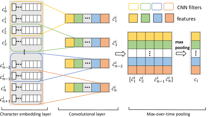
Specifically, the -th character in the word containing characters is firstly represented as an embedding vector in a similar manner as Eq. 1, except that the character embedding dictionary is initialized randomly. Then we use a convolutional layer to involve the information of neighboring characters for each character, which is critical to exploiting n-gram features. Finally, we perform a max-over-time pooling operation to reduce the convolution results into a single embedding vector :
| (2) | ||||
where is the kernel size of the convolutional layer. Here we fix as (?).
Note that RNNs, especially LSTMs/BiLSTMs are also suitable to model the character-level feature. However, as revealed in (?), CNNs are as powerful as RNNs in modelling the character-level feature. Besides, CNNs can probably enjoy higher training and test speed than RNNs. Therefore, in this paper we just adopt a CNN to model the character-level feature.
We regard as the character-level feature for the word . then we concatenate it to the word-level feature to derive the final word feature .
Context Layer
Context layer aims to model the local context information among neighboring words for each word. The local context is critical for predicting labels, regarding that there could exist strong dependencies among neighboring words in a sentence. For example, a location word often co-occurs with prepositions like in, on, at. Therefore, it is of necessity to capture the local context information for each word.
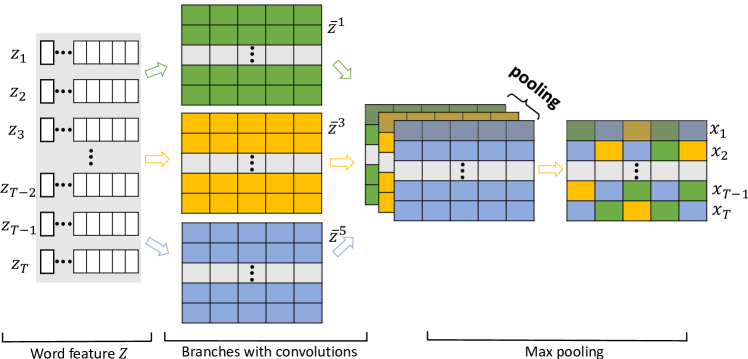
And it is obvious that the local dependencies are not limited within a certain distance. Therefore, we should enable the context layer to be adaptive to different scales of local information. Here, like InceptionNet (?), we design the context layer with different branches, each being comprised of one certain convolutionaly layer. Figure 2 shows the computational process of the context layer.
Specifically, we use three convolutional layers with the kernel size being 1, 3, 5, respectively. After obtaining the word feature of a sentence , each branch firstly extracts the local information within a window-size for each word . Then a max-pooling operation is employed to select the strongest channel-wise signals from all branches. To add the non-linear characteristic, we also apply tanh after each branch.
| (3) | ||||
where is the kernel size. For each , we use zero-paddings to ensure that each word can get the corresponding context feature. Here, we consider the output of the context layer as the context feature for word .
Although with various kernel sizes, the context layer can capture different kinds of local context information, it still struggles to capture the global one. However, we will show that with the gated relation layer described in the following subsection, the global context information can be realized by a fusion of the local one, thus tackling the shortcoming of the context layer.
Relation Layer
It has been shown that both short-term and long-term context information in a sequence is very critical in sequence learning tasks. LSTMs leverage the memory and the gating mechanism (?) to capture both context information and gain significant success. However, conventional CNNs cannot well capture the long-term context information owing to the limited receptive fields, and thus existing CNN-based NER models cannot achieve comparable performance as LSTM-based ones.
In this subsection, we introduce the gated relation layer in our proposed GRN, which aims to enhance the conventional CNNs with global context information. Specifically, it models the relations between any two words in the sentence. Then, with the gating mechanism, it composes a global context feature vector by weighted-summing up the relation scores with their corresponding local context feature vectors, as shown in Figure 3. Similar to the attention mechanism, our proposed GRN is effective in modelling long-term dependencies without regard to the limited CNN receptive fields. And importantly, GRN can allow computations to be performed in parallel across the entire sentence, which can generally help to reduce the time costs for training and test.
Given the local context features from the context layer for a sentence , the relation layer firstly computes the relation score vector between any two words and , which is of the same dimension as any . Specifically, it firstly concatenates the corresponding context features and , and then uses a linear function with the weight matrix and the bias vector to obtain :
| (4) |
Like (?), we can directly average these relation score vectors as follows:
| (5) |
where is the fused global context feature vector for the word by the direct feature fusion operation, i.e., averaging in Eq. 5. However, considering that non-entity words generally take up the majority of a sentence, this operation may introduce much noise and mislead the label prediction. To tackle that, we further introduce the gating mechanism, and enable the relation layer to learn to select other dependent words adaptively. Specifically, for the word , we firstly normalize all its relation score vectors with a sigmoid function to reduce their biases. Then we sum up the normalized relation score vectors with the corresponding local context feature vector of any other word . And similar to Eq. 5, finally we normalize the sum by the length of the sentence, i.e., .
| (6) |
where is a gate using sigmoid function, and means element-wise multiplication. Note that is asymmetrical and different from , and the relation vector w.r.t itself, i.e., , is also incorporated in the equation above. Therefore, with consisting of all the information of other words in the sentence, it can be seen as the global context feature vector for .
In a way, GRN can be seen as a channel-wise attention mechanism (?). However, instead of using a softmax function, we leverage the gating mechanism on the relation score vectors to decide how all the words play a part in predicting the label for the word . We can also customize Eq. 6 to the formula of attention with gating mechanism, where a gate is used to compute the attention weight for a word:
| (7) | ||||
where is an attention weight rather than a vector.
To distinguish from the proposed GRN (i.e., Eq. 6), we name Eq. 5 as Direct Fusion Network (DFN) and Eq. 7 as Gated Attention Network (GAttN). We will consider DFN and GAttN as two of our baseline models to show the superiority of the proposed GRN.

Here we also add a non-linear function for as follows.
| (8) |
And we define as the final predicting feature for word .
CRF Layer
Modelling label dependencies is crucial for NER task (?; ?). Following (?; ?), we employ a conditional random field (CRF) layer to model the label dependencies and calculate the loss for training GRN.
Formally, for a given sentence and its generic sequence of labels , we firstly use to denote the set of all possible label sequences for . The CRF model defines a family of conditional probability over all possible label sequences given :
| (9) |
where with being a function that maps words into labels:
| (10) |
where is derived as Eq. 8, is the predicting weights w.r.t and is the transition weight from to . Both and are parameters to be learned.
Loss of the CRF layer is formulated as follows.
| (11) |
And for decoding, we aim to find the label sequence with the highest conditional probability:
| (12) |
which can be efficiently derived via Viterbi decoding.
Experiments
To verify the effectiveness of the proposed GRN, we conduct extensive experiments on two benchmark NER datasets: CoNLL-2003 English NER (?) and OntoNotes 5.0 (?; ?).
-
•
CoNLL-2003 English NER consists of 22,137 sentences totally and is split into 14,987, 3,466 and 3,684 sentences for the training set, the development set and the test set, respectively. It includes annotations for 4 types of named entities: PERSON, LOCATION, ORGANIZATION and MISC.
-
•
OntoNotes 5.0 consists of much more (76,714) sentences from a wide variety of sources (telephone conversation, newswire, etc.). Following (?), we use the portion of the dataset with gold-standard named entity annotations, and thus excluded the New Testaments portion. It also contains much more kinds of entities, including CARDINAL, MONEY, LOC, PRODUCT, etc.
Table 1 shows some statistics of both datasets. Following (?), we use the BIOES sequence labelling scheme instead of BIO for both datasets to train models. As for test, we convert the prediction results back to the BIO scheme and use the standard CoNLL-2003 evaluation script to measure the NER performance, i.e., scores, etc.
dataset Train Dev Test CoNLL-2003 Sentence 14,987 3,466 3,684 Token 204,567 51,578 46,666 Entity 23,499 5,942 5,648 OntoNotes 5.0 Sentence 59,924 8,528 8,262 Token 1,088,503 147,724 152,728 Entity 81,828 11,066 11,257
Network Training
We implement our proposed GRN with the Pytorch library (?). And we set the parameters below following (?).
Word Embeddings. The dimension of word embedding is set as . And as mentioned, we initialize it with Stanford’s publicly available GloVe 100-dimensional embeddings. We include all words of GloVe when building the vocabulary, besides those words appearing at least times in the training set. For words out of the vocabulary (denoted as UNK) or those not in GloVe, we initialize their embeddings with kaiming uniform initialization (?).
Character Embeddings. We set the dimension of character embeddings as , and also initialize them with kaiming uniform initialization.
Weight Matrices and Bias Vectors. All weight matrices in linear functions and CNNs are initialized with kaiming uniform initialization, while bias vectors are initialized as .
Optimization. We employ mini-batch stochastic gradient descent with momentum to train the model. The batch size is set as . The momentum is set as and the initial learning rate is set as . We use learning rate decay strategy to update the learning rate during training. Namely, we update the learning rate as at the -th epoch with . We train each model on training sets with epochs totally, using dropout = . For evaluation, we select its best version with the highest performance on the development set and report the corresponding performance on the test set. To reduce the model bias, we carry out 5 runs for each model and report the average performance and the standard deviation.
Network Structure. The output channel number of the CNN in Eq. 2 and Eq. 3 is set as 30 and 400, respectively.
Model Mean() Max Mean P/R (?) 88.67 (?) 89.90 (?) 90.91 0.20 90.75 / 91.08 (?) 88.12 (?) 84.09 (?) 90.94 (?) 91.21 91.35 / 91.06 (?) 86.26 (?) 89.83 (?) 89.5 (?) 90.87 (?) 91.24 0.12 91.35 (?) 91.38 0.10 91.53 ID-CNN (?) 90.54 0.18 CNN-BiLSTM-CRF 91.17 0.18 91.45 CNN-BiLSTM-Att-CRF 90.24 0.15 90.48 GRN 91.44 0.16 91.67 91.31 / 91.57 (?)* 89.59 (?)* 91.2 (?)* 91.62 0.33 91.39 / 91.85 (?)* 91.93 0.19 (Tran et al. 2010)* 91.66 (Yang et al. 2017)* 91.26 (?)* 92.22 0.10 GRN* 92.34 0.10 92.45 92.04 / 92.65
Performance Comparison
Here we first focus on the NER performance comparison between the proposed GRN and the existing state-of-the-art approaches.
CoNLL-2003. We compare GRN with various state-of-the-art LSTM-based NER models, including (?; ?), etc. We also compare GRN with ID-CNN (?), which also adopts CNNs without recurrent layers for NER. Furthermore, considering that some state-of-the-art NER models exploit external knowledge to boost their performance, here we also report the performance of GRN with ELMo (?) incorporated as the external knowledge. Note that ELMo is trained on a large corpus of text data and can generate dynamic contextual features for words in a sentence. Here we simply concatenate the output ELMo features to the word feature in GRN. The experimental results are reported in Table 2, which also includes the max scores, mean precision and recall values if available. Note that CNN-BiLSTM-CRF is our re-implementation of (?), and we obtain comparable performance as that reported in the paper. Therefore, by default we directly compare GRN with the reported performance of compared baselines. It should also be noticed that, since the relation layer in GRN can be related to the attention mechanism, here we also include some attention-based baselines, i.e.,, (?) and (?), and we further introduce a new baseline termed CNN-BiLSTM-Att-CRF, which adds a self-attention layer for CNN-BiLSTM-CRF as (?).
As shown in Table 2, compared with those LSTM-based NER models, the proposed GRN can obtain comparable or even slightly superior performance, with or without the external knowledge, which well demonstrates the effectiveness of GRN. And compared with ID-CNN, our proposed GRN can defeat it at a great margin in terms of score. We also try to add ELMo to the latest state-of-the-art model of (?) based on their published codes, and we find that the corresponding score is , which is substantially lower than that of GRN.
OntoNotes 5.0. On OntoNotes 5.0, we compare the proposed GRN with NER models that also reported performance on it, including (?; ?; ?), etc. As shown in Table 3, GRN can obtain the state-of-the-art NER performance on OntoNotes 5.0, which further demonstrates its effectiveness.
Model Mean() Mean P/R (?) 86.28 0.26 86.04 / 86.53 (?) 86.63 0.49 (?) 84.04 85.22 / 82.89 (?) 82.30 (?) 83.45 CNN-BiLSTM-Att-CRF 87.250.17 ID-CNN (?) 86.84 0.19 GRN 87.67 0.17 87.79 / 87.56
Model Mean() Drop context GRN w/o context 88.36 0.21 3.08 GRN w/ 90.88 0.22 0.56 relation GRN w/o relation 90.13 0.28 1.31 DFN 90.72 0.06 0.72 GAttN 87.11 0.25 4.33 Full GRN 91.44 0.16 0
Model Mean() Drop context GRN w/o context 82.21 0.23 5.46 GRN w/ 86.66 0.21 1.01 relation GRN w/o relation 85.87 0.16 1.8 DFN 85.81 0.14 1.86 GAttN 79.83 0.37 7.83 Full GRN 87.67 0.17 0
Overall, the comparison results on both CoNLL-2003 and OntoNotes 5.0 well indicate that our proposed GRN can achieve state-of-the-art NER performance with or without external knowledge. It demonstrates that, using GRN, CNN-based models can compete with LSTM-based ones for NER.
Ablation Study
Here we study the impact of each layer on GRN. Firstly, we analyze the context layer by introducing two baseline models: (1) GRN w/o context: wiping out the context layer and building the relation layer on top of the representation layer directly; (2) GRN w/ : removing branches in the context layer, except the one with kernel size . Then to analyze the relation layer and the importance of gating mechanism in it, we compare GRN with: (1) GRN w/o relation: wiping out the relation layer and directly building the CRF layer on top of the context feature; (2) DFN (see Eq. 5); (3) GAttN (see Eq. 7). All compared baselines use the same experimental settings as GRN. Table 4 and Table 5 report the experimental results on both datasets, where the last column shows the absolute performance drops compared to GRN.

As shown in Table 4 and Table 5, when reducing the number of branches in the context layer, GRN w/o context and GRN w/ drop significantly, which indicates that modelling different scales of local context information plays a crucial role for NER.
Compared with GRN w/o relation, DFN and GAttN, the proposed GRN defeats them at a substantial margin in terms of score, which demonstrates that the proposed gated relation layer is beneficial to the performance improvement. The comparison also reveals that the channel-wise gating mechanism in GRN is more powerful than the gated attention approach (i.e., Eq. 7) and the direct fusion approach (i.e., Eq. 5) under the same experimental settings for NER.
Training/Test Time Comparison
In this section, we further compare the training and test time costs of the proposed GRN with those of CNN-BiLSTM-CRF, which is the most basic LSTM-based NER model achieving high performance. We conduct our experiments on a physical machine with Ubuntu 16.04, 2 Intel Xeon E5-2690 v4 CPUs, and a Tesla P100 GPU. For fair comparison, we keep the representation layer and the CRF layer the same for both models, so that the input and output dimensions for the “BiLSTM layer” in CNN-BiLSTM-CRF would be identical to those of the “context layer + relation layer” in GRN. We train both models with random initialization for a total of 30 epochs, and after each epoch, we evaluate the learned model on the test set. For both training and test, batch size is set as as before. And here we use the average training time per epoch and the average test time to calculate speedups.
As shown in Table 6, GRN can obtain a speedup of more than during training and around during test on both datasets. The speedup may seem not so significant, because the time costs reported here also include those consumed by common representation layer, CRF layer, etc. For reference, the fast ID-CNN with a CRF layer (i.e., ID-CNN-CRF) (?) was reported to have a test-time speedup of over the basic BiLSTM-CRF model on CoNLL-2003. Compared to ID-CNN-CRF, GRN sacrifices some speedup for better performance, and the speedup gap between both is still reasonable. We can also see that the speedup on CoNLL-2003 is larger than that on OntoNotes 5.0, which can be attributed to that the average sentence length of CoNLL-2003 () is smaller than that of OntoNotes 5.0 () and thus the relation layer in GRN would cost less time for the former. The results above demonstrate that the proposed GRN can generally bring efficiency improvement over LSTM-based methods for NER, via fully exploiting the GPU parallelism.
CoNLL-2003 OntoNotes 5.0 Training 1.16x 1.15x Test 1.19x 1.08x
Word Relation Visualization
Since the proposed GRN aims to boost the NER performance by modelling the relations between words, especially long-term ones, we can visualize the gating output in the relation layer to illustrate the interpretability of GRN. Specifically, we utilize the norm of to indicate the extent of relations between the word and the word . Then we further normalize the values into to build a heat map. Figure 4 shows a visualization sample. We can find out that the entity words (y-axis) are more related to other entity words as well, even though they may be “far away” from each other in the sentence, like the 1st word “Sun” and the 8th word “Sidek” in the sample. Note that “Sun” and “Sidek” are not in an identical receptive field of any CNN used in our experiments, but their strong correlation can still be exploited with the relation layer in GRN. That concretely illustrates that, by introducing the gated relation layer, GRN is able to capture the long-term dependency between words.
Conclusion
In this paper, we propose a CNN-based network, i.e., gated relation network (GRN), for named entity recognition (NER). Unlike the dominant LSTM-based NER models which process a sentence in a sequential manner, GRN can process all the words concurrently with one forward operation and thus can fully exploit the GPU parallelism for potential efficiency improvement. Besides, compared with common CNNs, GRN has a better capacity of capturing long-term context information. Specifically, GRN introduces a gated relation layer to model the relations between any two words, and utilizes gating mechanism to fuse local context features into global ones for all words. Experiments on CoNLL-2003 English NER and Ontonotes 5.0 datasets show that, GRN can achieve state-of-the-art NER performance with or without external knowledge, meaning that using GRN, CNN-based models can compete with LSTM-based models for NER. Experimental results also show that GRN can generally bring efficiency improvement for training and test.
Acknowledgements
This work is supported by the National Natural Science Foundation of China (No. 61571269).
References
- [Bikel et al. 1997] Bikel, D. M.; Miller, S.; Schwartz, R.; and Weischedel, R. 1997. Nymble: a high-performance learning name-finder. In ANLP, 194–201.
- [Chen et al. 2017] Chen, L.; Zhang, H.; Xiao, J.; Nie, L.; Shao, J.; Liu, W.; and Chua, T.-S. 2017. Sca-cnn: Spatial and channel-wise attention in convolutional networks for image captioning. In CVPR, 6298–6306.
- [Chiu and Nichols 2016] Chiu, J., and Nichols, E. 2016. Named entity recognition with bidirectional lstm-cnns. TACL 4(1):357–370.
- [Collobert et al. 2011] Collobert, R.; Weston, J.; Bottou, L.; Karlen, M.; Kavukcuoglu, K.; and Kuksa, P. 2011. Natural language processing (almost) from scratch. JMLR 12:2493–2537.
- [Durrett and Klein 2014] Durrett, G., and Klein, D. 2014. A joint model for entity analysis: Coreference, typing, and linking. TACL 2(1):477–490.
- [Gehring et al. 2017] Gehring, J.; Auli, M.; Grangier, D.; Yarats, D.; and Dauphin, Y. N. 2017. Convolutional sequence to sequence learning. In ICML, 1243–1252.
- [He et al. 2015] He, K.; Zhang, X.; Ren, S.; and Sun, J. 2015. Delving deep into rectifiers: Surpassing human-level performance on imagenet classification. In ICCV, 1026–1034.
- [Hochreiter and Schmidhuber 1997] Hochreiter, S., and Schmidhuber, J. 1997. Long short-term memory. Neural Computation 9(8):1735–1780.
- [Hovy et al. 2006] Hovy, E.; Marcus, M.; Palmer, M.; Ramshaw, L.; and Weischedel, R. 2006. Ontonotes: the 90% solution. In NAACL-HLT, 57–60.
- [Huang, Xu, and Yu 2015] Huang, Z.; Xu, W.; and Yu, K. 2015. Bidirectional lstm-crf models for sequence tagging. arXiv:1508.01991.
- [Lample et al. 2016] Lample, G.; Ballesteros, M.; Subramanian, S.; Kawakami, K.; and Dyer, C. 2016. Neural architectures for named entity recognition. In NAACL-HLT, 260–270.
- [Liu, Baldwin, and Cohn 2017] Liu, F.; Baldwin, T.; and Cohn, T. 2017. Capturing long-range contextual dependencies with memory-enhanced conditional random fields. In IJCNLP, 555–565.
- [Liu et al. 2018] Liu, L.; Shang, J.; Xu, F.; Ren, X.; Gui, H.; Peng, J.; and Han, J. 2018. Empower Sequence Labeling with Task-Aware Neural Language Model. In AAAI.
- [Luo et al. 2015] Luo, G.; Huang, X.; Lin, C.-Y.; and Nie, Z. 2015. Joint entity recognition and disambiguation. In EMNLP, 879–888.
- [Ma and Hovy 2016] Ma, X., and Hovy, E. 2016. End-to-end sequence labeling via bi-directional lstm-cnns-crf. In ACL, 1064–1074.
- [McCallum and Li 2003] McCallum, A., and Li, W. 2003. Early results for named entity recognition with conditional random fields, feature induction and web-enhanced lexicons. In CoNLL, 188–191.
- [Passos, Kumar, and McCallum 2014] Passos, A.; Kumar, V.; and McCallum, A. 2014. Lexicon infused phrase embeddings for named entity resolution. In CoNLL, 78–86.
- [Paszke et al. 2017] Paszke, A.; Gross, S.; Chintala, S.; Chanan, G.; Yang, E.; DeVito, Z.; Lin, Z.; Desmaison, A.; Antiga, L.; and Lerer, A. 2017. Automatic differentiation in pytorch. In NIPS.
- [Pennington, Socher, and Manning 2014] Pennington, J.; Socher, R.; and Manning, C. 2014. Glove: Global vectors for word representation. In EMNLP, 1532–1543.
- [Peters et al. 2017] Peters, M.; Ammar, W.; Bhagavatula, C.; and Power, R. 2017. Semi-supervised sequence tagging with bidirectional language models. In ACL, 1756–1765.
- [Peters et al. 2018] Peters, M.; Neumann, M.; Iyyer, M.; Gardner, M.; Clark, C.; Lee, K.; and Zettlemoyer, L. 2018. Deep contextualized word representations. In NAACL-HLT, 2227–2237.
- [Pradhan et al. 2013] Pradhan, S.; Moschitti, A.; Xue, N.; Ng, H. T.; Björkelund, A.; Uryupina, O.; Zhang, Y.; and Zhong, Z. 2013. Towards robust linguistic analysis using ontonotes. In CoNLL, 143–152.
- [Rei, Crichton, and Pyysalo 2016] Rei, M.; Crichton, G.; and Pyysalo, S. 2016. Attending to characters in neural sequence labeling models. In COLING, 309–318.
- [Rei 2017] Rei, M. 2017. Semi-supervised multitask learning for sequence labeling. In ACL, 2121–2130.
- [Santoro et al. 2017] Santoro, A.; Raposo, D.; Barrett, D. G.; Malinowski, M.; Pascanu, R.; Battaglia, P.; and Lillicrap, T. 2017. A simple neural network module for relational reasoning. In NIPS, 4967–4976.
- [Shen et al. 2017] Shen, Y.; Yun, H.; Lipton, Z.; Kronrod, Y.; and Anandkumar, A. 2017. Deep active learning for named entity recognition. In Workshop on Representation Learning for NLP, 252–256.
- [Strubell et al. 2017] Strubell, E.; Verga, P.; Belanger, D.; and McCallum, A. 2017. Fast and accurate entity recognition with iterated dilated convolutions. In EMNLP, 2670–2680.
- [Szegedy et al. 2015] Szegedy, C.; Liu, W.; Jia, Y.; Sermanet, P.; Reed, S.; Anguelov, D.; Erhan, D.; Vanhoucke, V.; and Rabinovich, A. 2015. Going deeper with convolutions. In CVPR, 1–9.
- [Tjong Kim Sang and De Meulder 2003] Tjong Kim Sang, E. F., and De Meulder, F. 2003. Introduction to the conll-2003 shared task: Language-independent named entity recognition. In CoNLL, 142–147.
- [Tran, MacKinlay, and Yepes 2017] Tran, Q.; MacKinlay, A.; and Yepes, A. J. 2017. Named entity recognition with stack residual lstm and trainable bias decoding. In IJCNLP, 566–575.
- [Vaswani et al. 2017] Vaswani, A.; Shazeer, N.; Parmar, N.; Uszkoreit, J.; Jones, L.; Gomez, A. N.; Kaiser, Ł.; and Polosukhin, I. 2017. Attention is all you need. In NIPS, 5998–6008.
- [Yang, Liang, and Zhang 2018] Yang, J.; Liang, S.; and Zhang, Y. 2018. Design challenges and misconceptions in neural sequence labeling. In COLING, 3879–3889.
- [Yang, Salakhutdinov, and Cohen 2017] Yang, Z.; Salakhutdinov, R.; and Cohen, W. W. 2017. Transfer learning for sequence tagging with hierarchical recurrent networks. arXiv:1703.06345.
- [Ye and Ling 2018] Ye, Z., and Ling, Z.-H. 2018. Hybrid semi-markov crf for neural sequence labeling. In ACL, 235–240.
- [Zhuo et al. 2016] Zhuo, J.; Cao, Y.; Zhu, J.; Zhang, B.; and Nie, Z. 2016. Segment-level sequence modeling using gated recursive semi-markov conditional random fields. In ACL, 1413–1423.
- [Zukov-Gregoric et al. 2017] Zukov-Gregoric, A.; Bachrach, Y.; Minkovsky, P.; Coope, S.; and Maksak, B. 2017. Neural named entity recognition using a self-attention mechanism. In ICTAI, 652–656.