Generative Modeling by Estimating Gradients of the Data Distribution

Abstract

We introduce a new generative model where samples are produced via Langevin dynamics using gradients of the data distribution estimated with score matching. Because gradients can be ill-defined and hard to estimate when the data resides on low-dimensional manifolds, we perturb the data with different levels of Gaussian noise, and jointly estimate the corresponding scores, i.e., the vector fields of gradients of the perturbed data distribution for all noise levels. For sampling, we propose an annealed Langevin dynamics where we use gradients corresponding to gradually decreasing noise levels as the sampling process gets closer to the data manifold. Our framework allows flexible model architectures, requires no sampling during training or the use of adversarial methods, and provides a learning objective that can be used for principled model comparisons. Our models produce samples comparable to GANs on MNIST, CelebA and CIFAR-10 datasets, achieving a new state-of-the-art inception score of 8.87 on CIFAR-10. Additionally, we demonstrate that our models learn effective representations via image inpainting experiments.

1 Introduction

Generative models have many applications in machine learning. To list a few, they have been used to generate high-fidelity images [26, 6], synthesize realistic speech and music fragments [58], improve the performance of semi-supervised learning [28, 10], detect adversarial examples and other anomalous data [54], imitation learning [22], and explore promising states in reinforcement learning [41]. Recent progress is mainly driven by two approaches: likelihood-based methods [17, 29, 11, 60] and generative adversarial networks (GAN [15]). The former uses log-likelihood (or a suitable surrogate) as the training objective, while the latter uses adversarial training to minimize $f$-divergences [40] or integral probability metrics [2, 55] between model and data distributions.

Although likelihood-based models and GANs have achieved great success, they have some intrinsic limitations. For example, likelihood-based models either have to use specialized architectures to build a normalized probability model (e.g., autoregressive models, flow models), or use surrogate losses (e.g., the evidence lower bound used in variational auto-encoders [29], contrastive divergence in energy-based models [21]) for training. GANs avoid some of the limitations of likelihood-based models, but their training can be unstable due to the adversarial training procedure. In addition, the GAN objective is not suitable for evaluating and comparing different GAN models. While other objectives exist for generative modeling, such as noise contrastive estimation [19] and minimum probability flow [50], these methods typically only work well for low-dimensional data.

In this paper, we explore a new principle for generative modeling based on estimating and sampling from the (Stein) score [33] of the logarithmic data density, which is the gradient of the log-density function at the input data point. This is a vector field pointing in the direction where the log data density grows the most. We use a neural network trained with score matching [24] to learn this vector field from data. We then produce samples using Langevin dynamics, which approximately works by gradually moving a random initial sample to high density regions along the (estimated) vector field of scores. However, there are two main challenges with this approach. First, if the data distribution is supported on a low dimensional manifold—as it is often assumed for many real world datasets—the score will be undefined in the ambient space, and score matching will fail to provide a consistent score estimator. Second, the scarcity of training data in low data density regions, e.g., far from the manifold, hinders the accuracy of score estimation and slows down the mixing of Langevin dynamics sampling. Since Langevin dynamics will often be initialized in low-density regions of the data distribution, inaccurate score estimation in these regions will negatively affect the sampling process. Moreover, mixing can be difficult because of the need of traversing low density regions to transition between modes of the distribution.

To tackle these two challenges, we propose to perturb the data with random Gaussian noise of various magnitudes. Adding random noise ensures the resulting distribution does not collapse to a low dimensional manifold. Large noise levels will produce samples in low density regions of the original (unperturbed) data distribution, thus improving score estimation. Crucially, we train a single score network conditioned on the noise level and estimate the scores at all noise magnitudes. We then propose an annealed version of Langevin dynamics, where we initially use scores corresponding to the highest noise level, and gradually anneal down the noise level until it is small enough to be indistinguishable from the original data distribution. Our sampling strategy is inspired by simulated annealing [30, 37] which heuristically improves optimization for multimodal landscapes.

Our approach has several desirable properties. First, our objective is tractable for almost all parameterizations of the score networks without the need of special constraints or architectures, and can be optimized without adversarial training, MCMC sampling, or other approximations during training. The objective can also be used to quantitatively compare different models on the same dataset. Experimentally, we demonstrate the efficacy of our approach on MNIST, CelebA [34], and CIFAR-10 [31]. We show that the samples look comparable to those generated from modern likelihood-based models and GANs. On CIFAR-10, our model sets the new state-of-the-art inception score of 8.87 for unconditional generative models, and achieves a competitive FID score of 25.32. We show that the model learns meaningful representations of the data by image inpainting experiments.

2 Score-based generative modeling

Suppose our dataset consists of i.i.d. samples $\{\mathbf{x}_{i}\in\mathbb{R}^{D}\}_{i=1}^{N}$ from an unknown data distribution $p_{\text{data}}(\mathbf{x})$. We define the score of a probability density $p(\mathbf{x})$ to be $\nabla_{\mathbf{x}}\log p(\mathbf{x})$. The score network $\mathbf{s}_{\boldsymbol{\theta}}:\mathbb{R}^{D}\rightarrow\mathbb{R}^{D}$ is a neural network parameterized by ${\boldsymbol{\theta}}$, which will be trained to approximate the score of $p_{\text{data}}(\mathbf{x})$. The goal of generative modeling is to use the dataset to learn a model for generating new samples from $p_{\text{data}}(\mathbf{x})$. The framework of score-based generative modeling has two ingredients: score matching and Langevin dynamics.

2.1 Score matching for score estimation

Score matching [24] is originally designed for learning non-normalized statistical models based on i.i.d. samples from an unknown data distribution. Following [53], we repurpose it for score estimation. Using score matching, we can directly train a score network $\mathbf{s}_{\boldsymbol{\theta}}(\mathbf{x})$ to estimate $\nabla_{\mathbf{x}}\log p_{\text{data}}(\mathbf{x})$ without training a model to estimate $p_{\text{data}}(\mathbf{x})$ first. Different from the typical usage of score matching, we opt not to use the gradient of an energy-based model as the score network to avoid extra computation due to higher-order gradients. The objective minimizes $\frac{1}{2}\mathbb{E}_{p_{\text{data}}}[\left\lVert\mathbf{s}_{\boldsymbol{\theta}}(\mathbf{x})-\nabla_{\mathbf{x}}\log p_{\text{data}}(\mathbf{x})\right\rVert_{2}^{2}]$, which can be shown equivalent to the following up to a constant

$$\mathbb{E}_{p_{\text{data}}(\mathbf{x})}\bigg{[}\operatorname{tr}(\nabla_{\mathbf{x}}\mathbf{s}_{\boldsymbol{\theta}}(\mathbf{x}))+\frac{1}{2}\left\lVert\mathbf{s}_{\boldsymbol{\theta}}(\mathbf{x})\right\rVert_{2}^{2}\bigg{]},$$ (1)

where $\nabla_{\mathbf{x}}\mathbf{s}_{\boldsymbol{\theta}}(\mathbf{x})$ denotes the Jacobian of $\mathbf{s}_{\boldsymbol{\theta}}(\mathbf{x})$. As shown in [53], under some regularity conditions the minimizer of Eq. (3) (denoted as $\mathbf{s}_{{\boldsymbol{\theta}}^{*}}(\mathbf{x})$) satisfies $\mathbf{s}_{{\boldsymbol{\theta}}^{*}}(\mathbf{x})=\nabla_{\mathbf{x}}\log p_{\text{data}}(\mathbf{x})$ almost surely. In practice, the expectation over $p_{\text{data}}(\mathbf{x})$ in Eq. (1) can be quickly estimated using data samples. However, score matching is not scalable to deep networks and high dimensional data [53] due to the computation of $\operatorname{tr}(\nabla_{\mathbf{x}}\mathbf{s}_{\boldsymbol{\theta}}(\mathbf{x}))$. Below we discuss two popular methods for large scale score matching.

Denoising score matching

Denoising score matching [61] is a variant of score matching that completely circumvents $\operatorname{tr}(\nabla_{\mathbf{x}}\mathbf{s}_{\boldsymbol{\theta}}(\mathbf{x}))$. It first perturbs the data point $\mathbf{x}$ with a pre-specified noise distribution $q_{\sigma}(\tilde{\mathbf{x}}\mid\mathbf{x})$ and then employs score matching to estimate the score of the perturbed data distribution $q_{\sigma}(\tilde{\mathbf{x}})\triangleq\int q_{\sigma}(\tilde{\mathbf{x}}\mid\mathbf{x})p_{\text{data}}(\mathbf{x})\mathrm{d}\mathbf{x}$. The objective was proved equivalent to the following:

$$\frac{1}{2}\mathbb{E}_{q_{\sigma}(\tilde{\mathbf{x}}\mid\mathbf{x})p_{\text{data}}(\mathbf{x})}[\|\mathbf{s}_{\boldsymbol{\theta}}(\tilde{\mathbf{x}})-\nabla_{\tilde{\mathbf{x}}}\log q_{\sigma}(\tilde{\mathbf{x}}\mid\mathbf{x})\|_{2}^{2}].$$ (2)

As shown in [61], the optimal score network (denoted as $\mathbf{s}_{{\boldsymbol{\theta}}^{*}}(\mathbf{x})$) that minimizes Eq. (2) satisfies $\mathbf{s}_{{\boldsymbol{\theta}}^{*}}(\mathbf{x})=\nabla_{\mathbf{x}}\log q_{\sigma}(\mathbf{x})$ almost surely. However, $\mathbf{s}_{{\boldsymbol{\theta}}^{*}}(\mathbf{x})=\nabla_{\mathbf{x}}\log q_{\sigma}(\mathbf{x})\approx\nabla_{\mathbf{x}}\log p_{\text{data}}(\mathbf{x})$ is true only when the noise is small enough such that $q_{\sigma}(\mathbf{x})\approx p_{\text{data}}(\mathbf{x})$.

Sliced score matching

Sliced score matching [53] uses random projections to approximate $\operatorname{tr}(\nabla_{\mathbf{x}}\mathbf{s}_{\boldsymbol{\theta}}(\mathbf{x}))$ in score matching. The objective is

$$\mathbb{E}_{p_{\mathbf{v}}}\mathbb{E}_{p_{\text{data}}}\bigg{[}\mathbf{v}^{\intercal}\nabla_{\mathbf{x}}\mathbf{s}_{\boldsymbol{\theta}}(\mathbf{x})\mathbf{v}+\frac{1}{2}\left\lVert\mathbf{s}_{\boldsymbol{\theta}}(\mathbf{x})\right\rVert_{2}^{2}\bigg{]},$$ (3)

where $p_{\mathbf{v}}$ is a simple distribution of random vectors, e.g., the multivariate standard normal. As shown in [53], the term $\mathbf{v}^{\intercal}\nabla_{\mathbf{x}}\mathbf{s}_{\boldsymbol{\theta}}(\mathbf{x})\mathbf{v}$ can be efficiently computed by forward mode auto-differentiation. Unlike denoising score matching which estimates the scores of perturbed data, sliced score matching provides score estimation for the original unperturbed data distribution, but requires around four times more computations due to the forward mode auto-differentiation.

2.2 Sampling with Langevin dynamics

Langevin dynamics can produce samples from a probability density $p(\mathbf{x})$ using only the score function $\nabla_{\mathbf{x}}\log p(\mathbf{x})$. Given a fixed step size $\epsilon>0$, and an initial value $\tilde{\mathbf{x}}_{0}\sim\pi(\mathbf{x})$ with $\pi$ being a prior distribution, the Langevin method recursively computes the following

$$\tilde{\mathbf{x}}_{t}=\tilde{\mathbf{x}}_{t-1}+\frac{\epsilon}{2}\nabla_{\mathbf{x}}\log p(\tilde{\mathbf{x}}_{t-1})+\sqrt{\epsilon}~{}\mathbf{z}_{t},$$ (4)

where $\mathbf{z}_{t}\sim\mathcal{N}(0,I)$. The distribution of $\tilde{\mathbf{x}}_{T}$ equals $p(\mathbf{x})$ when $\epsilon\rightarrow 0$ and $T\rightarrow\infty$, in which case $\tilde{\mathbf{x}}_{T}$ becomes an exact sample from $p(\mathbf{x})$ under some regularity conditions [62]. When $\epsilon>0$ and $T<\infty$, a Metropolis-Hastings update is needed to correct the error of Eq. (4), but it can often be ignored in practice [9, 12, 39]. In this work, we assume this error is negligible when $\epsilon$ is small and $T$ is large.

Note that sampling from Eq. (4) only requires the score function $\nabla_{\mathbf{x}}\log p(\mathbf{x})$. Therefore, in order to obtain samples from $p_{\text{data}}(\mathbf{x})$, we can first train our score network such that $\mathbf{s}_{\boldsymbol{\theta}}(\mathbf{x})\approx\nabla_{\mathbf{x}}\log p_{\text{data}}(\mathbf{x})$ and then approximately obtain samples with Langevin dynamics using $\mathbf{s}_{\boldsymbol{\theta}}(\mathbf{x})$. This is the key idea of our framework of score-based generative modeling.

3 Challenges of score-based generative modeling

In this section, we analyze more closely the idea of score-based generative modeling. We argue that there are two major obstacles that prevent a naïve application of this idea.

3.1 The manifold hypothesis

Figure 1: Left: Sliced score matching (SSM) loss w.r.t. iterations. No noise is added to data. Right: Same but data are perturbed with $\mathcal{N}(0,0.0001)$.

The manifold hypothesis states that data in the real world tend to concentrate on low dimensional manifolds embedded in a high dimensional space (a.k.a., the ambient space). This hypothesis empirically holds for many datasets, and has become the foundation of manifold learning [3, 47]. Under the manifold hypothesis, score-based generative models will face two key difficulties. First, since the score $\nabla_{\mathbf{x}}\log p_{\text{data}}(\mathbf{x})$ is a gradient taken in the ambient space, it is undefined when $\mathbf{x}$ is confined to a low dimensional manifold. Second, the score matching objective Eq. (1) provides a consistent score estimator only when the support of the data distribution is the whole space (cf., Theorem 2 in [24]), and will be inconsistent when the data reside on a low-dimensional manifold.

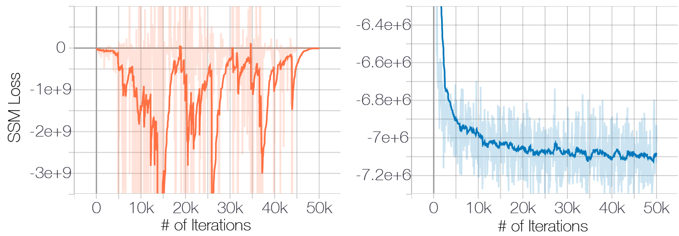
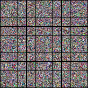
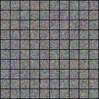
The negative effect of the manifold hypothesis on score estimation can be seen clearly from Fig. 1, where we train a ResNet (details in Appendix B.1) to estimate the data score on CIFAR-10. For fast training and faithful estimation of the data scores, we use the sliced score matching objective (Eq. (3)). As Fig. 1 (left) shows, when trained on the original CIFAR-10 images, the sliced score matching loss first decreases and then fluctuates irregularly. In contrast, if we perturb the data with a small Gaussian noise (such that the perturbed data distribution has full support over $\mathbb{R}^{D}$), the loss curve will converge (right panel). Note that the Gaussian noise $\mathcal{N}(0,0.0001)$ we impose is very small for images with pixel values in the range $[0,1]$, and is almost indistinguishable to human eyes.

3.2 Low data density regions

The scarcity of data in low density regions can cause difficulties for both score estimation with score matching and MCMC sampling with Langevin dynamics.

3.2.1 Inaccurate score estimation with score matching

Figure 2: Left: $\nabla_{\mathbf{x}}\log p_{\text{data}}(\mathbf{x})$; Right: $\mathbf{s}_{\boldsymbol{\theta}}(\mathbf{x})$. The data density $p_{\text{data}}(\mathbf{x})$ is encoded using an orange colormap: darker color implies higher density. Red rectangles highlight regions where $\nabla_{\mathbf{x}}\log p_{\text{data}}(\mathbf{x})\approx\mathbf{s}_{\boldsymbol{\theta}}(\mathbf{x})$.

In regions of low data density, score matching may not have enough evidence to estimate score functions accurately, due to the lack of data samples. To see this, recall from Section 2.1 that score matching minimizes the expected squared error of the score estimates, i.e., $\frac{1}{2}\mathbb{E}_{p_{\text{data}}}[\left\lVert\mathbf{s}_{\boldsymbol{\theta}}(\mathbf{x})-\nabla_{\mathbf{x}}\log p_{\text{data}}(\mathbf{x})\right\rVert_{2}^{2}]$. In practice, the expectation w.r.t. the data distribution is always estimated using i.i.d. samples $\{\mathbf{x}_{i}\}_{i=1}^{N}\stackrel{{\scriptstyle\text{i.i.d.\hbox{} missing}}}{{\sim}}p_{\text{data}}(\mathbf{x})$. Consider any region $\mathcal{R}\subset\mathbb{R}^{D}$ such that $p_{\text{data}}(\mathcal{R})\approx 0$. In most cases $\{\mathbf{x}_{i}\}_{i=1}^{N}\cap\mathcal{R}=\varnothing$, and score matching will not have sufficient data samples to estimate $\nabla_{\mathbf{x}}\log p_{\text{data}}(\mathbf{x})$ accurately for $\mathbf{x}\in\mathcal{R}$.

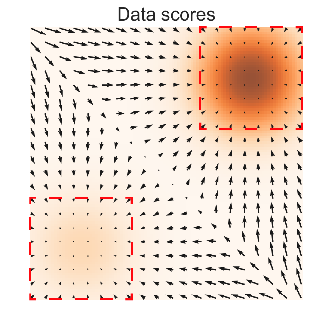
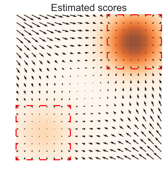
To demonstrate the negative effect of this, we provide the result of a toy experiment (details in Appendix B.1) in Fig. 2 where we use sliced score matching to estimate scores of a mixture of Gaussians $p_{\text{data}}=\frac{1}{5}\mathcal{N}((-5,-5),I)+\frac{4}{5}\mathcal{N}((5,5),I)$. As the figure demonstrates, score estimation is only reliable in the immediate vicinity of the modes of $p_{\text{data}}$, where the data density is high.

3.2.2 Slow mixing of Langevin dynamics

When two modes of the data distribution are separated by low density regions, Langevin dynamics will not be able to correctly recover the relative weights of these two modes in reasonable time, and therefore might not converge to the true distribution. Our analyses of this are largely inspired by [63], which analyzed the same phenomenon in the context of density estimation with score matching.

Figure 3: Samples from a mixture of Gaussian with different methods. (a) Exact sampling. (b) Sampling using Langevin dynamics with the exact scores. (c) Sampling using annealed Langevin dynamics with the exact scores. Clearly Langevin dynamics estimate the relative weights between the two modes incorrectly, while annealed Langevin dynamics recover the relative weights faithfully.

Consider a mixture distribution $p_{\text{data}}(\mathbf{x})=\pi p_{1}(\mathbf{x})+(1-\pi)p_{2}(\mathbf{x})$, where $p_{1}(\mathbf{x})$ and $p_{2}(\mathbf{x})$ are normalized distributions with disjoint supports, and $\pi\in(0,1)$. In the support of $p_{1}(\mathbf{x})$, $\nabla_{\mathbf{x}}\log p_{\text{data}}(\mathbf{x})=\nabla_{\mathbf{x}}(\log\pi+\log p_{1}(\mathbf{x}))=\nabla_{\mathbf{x}}\log p_{1}(\mathbf{x})$, and in the support of $p_{2}(\mathbf{x})$, $\nabla_{\mathbf{x}}\log p_{\text{data}}(\mathbf{x})=\nabla_{\mathbf{x}}(\log(1-\pi)+\log p_{2}(\mathbf{x}))=\nabla_{\mathbf{x}}\log p_{2}(\mathbf{x})$. In either case, the score $\nabla_{\mathbf{x}}\log p_{\text{data}}(\mathbf{x})$ does not depend on $\pi$. Since Langevin dynamics use $\nabla_{\mathbf{x}}\log p_{\text{data}}(\mathbf{x})$ to sample from $p_{\text{data}}(\mathbf{x})$, the samples obtained will not depend on $\pi$. In practice, this analysis also holds when different modes have approximately disjoint supports—they may share the same support but be connected by regions of small data density. In this case, Langevin dynamics can produce correct samples in theory, but may require a very small step size and a very large number of steps to mix.

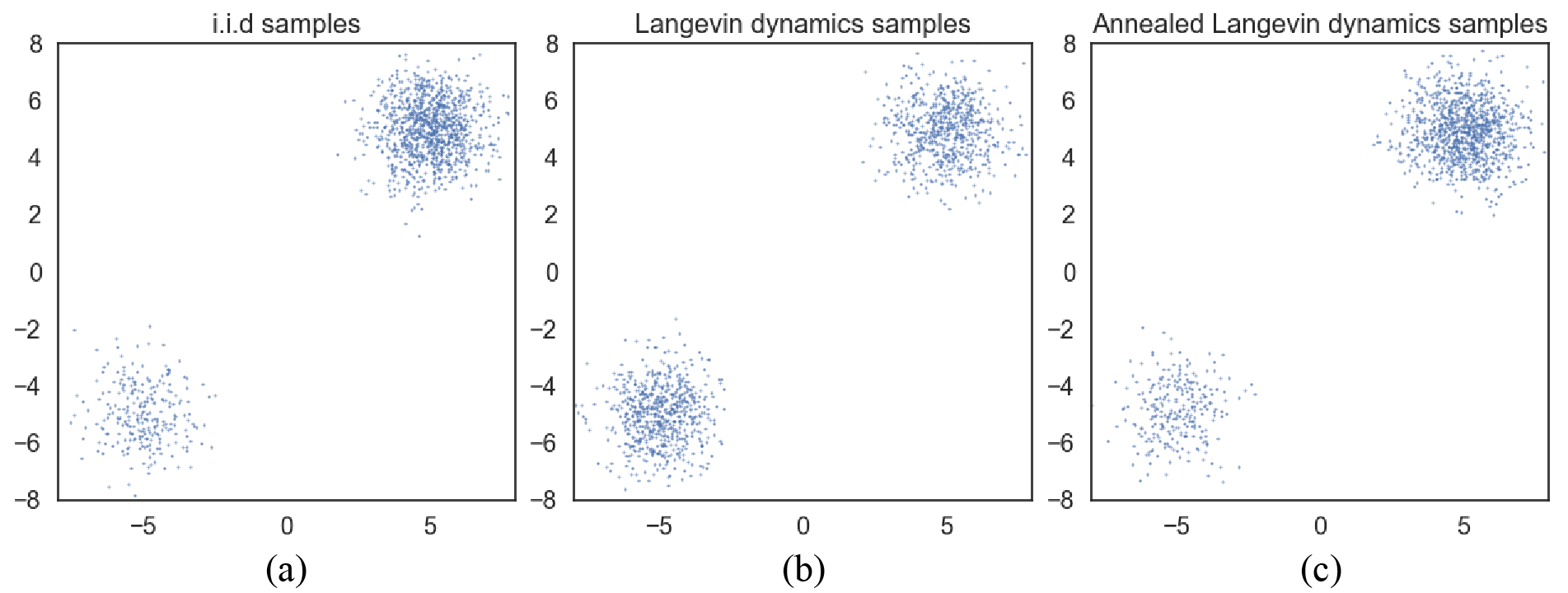
To verify this analysis, we test Langevin dynamics sampling for the same mixture of Gaussian used in Section 3.2.1 and provide the results in Fig. 3. We use the ground truth scores when sampling with Langevin dynamics. Comparing Fig. 3(b) with (a), it is obvious that the samples from Langevin dynamics have incorrect relative density between the two modes, as predicted by our analysis.

4 Noise Conditional Score Networks: learning and inference

We observe that perturbing data with random Gaussian noise makes the data distribution more amenable to score-based generative modeling. First, since the support of our Gaussian noise distribution is the whole space, the perturbed data will not be confined to a low dimensional manifold, which obviates difficulties from the manifold hypothesis and makes score estimation well-defined. Second, large Gaussian noise has the effect of filling low density regions in the original unperturbed data distribution; therefore score matching may get more training signal to improve score estimation. Furthermore, by using multiple noise levels we can obtain a sequence of noise-perturbed distributions that converge to the true data distribution. We can improve the mixing rate of Langevin dynamics on multimodal distributions by leveraging these intermediate distributions in the spirit of simulated annealing [30] and annealed importance sampling [37].

Built upon this intuition, we propose to improve score-based generative modeling by 1) perturbing the data using various levels of noise; and 2) simultaneously estimating scores corresponding to all noise levels by training a single conditional score network. After training, when using Langevin dynamics to generate samples, we initially use scores corresponding to large noise, and gradually anneal down the noise level. This helps smoothly transfer the benefits of large noise levels to low noise levels where the perturbed data are almost indistinguishable from the original ones. In what follows, we will elaborate more on the details of our method, including the architecture of our score networks, the training objective, and the annealing schedule for Langevin dynamics.

4.1 Noise Conditional Score Networks

Let $\{\sigma_{i}\}_{i=1}^{L}$ be a positive geometric sequence that satisfies $\frac{\sigma_{1}}{\sigma_{2}}=\cdots=\frac{\sigma_{L-1}}{\sigma_{L}}>1$. Let $q_{\sigma}(\mathbf{x})\triangleq\int p_{\text{data}}(\mathbf{t})\mathcal{N}(\mathbf{x}\mid\mathbf{t},\sigma^{2}I)\mathrm{d}\mathbf{t}$ denote the perturbed data distribution. We choose the noise levels $\{\sigma_{i}\}_{i=1}^{L}$ such that $\sigma_{1}$ is large enough to mitigate the difficulties discussed in Section 3, and $\sigma_{L}$ is small enough to minimize the effect on data. We aim to train a conditional score network to jointly estimate the scores of all perturbed data distributions, i.e., $\forall\sigma\in\{\sigma_{i}\}_{i=1}^{L}:\mathbf{s}_{\boldsymbol{\theta}}(\mathbf{x},\sigma)\approx\nabla_{\mathbf{x}}\log q_{\sigma}(\mathbf{x})$. Note that $\mathbf{s}_{\boldsymbol{\theta}}(\mathbf{x},\sigma)\in\mathbb{R}^{D}$ when $\mathbf{x}\in\mathbb{R}^{D}$. We call $\mathbf{s}_{\boldsymbol{\theta}}(\mathbf{x},\sigma)$ a Noise Conditional Score Network (NCSN).

Similar to likelihood-based generative models and GANs, the design of model architectures plays an important role in generating high quality samples. In this work, we mostly focus on architectures useful for image generation, and leave the architecture design for other domains as future work. Since the output of our noise conditional score network $\mathbf{s}_{\boldsymbol{\theta}}(\mathbf{x},\sigma)$ has the same shape as the input image $\mathbf{x}$, we draw inspiration from successful model architectures for dense prediction of images (e.g., semantic segmentation). In the experiments, our model $\mathbf{s}_{\boldsymbol{\theta}}(\mathbf{x},\sigma)$ combines the architecture design of U-Net [46] with dilated/atrous convolution [64, 65, 8]—both of which have been proved very successful in semantic segmentation. In addition, we adopt instance normalization in our score network, inspired by its superior performance in some image generation tasks [57, 13, 23], and we use a modified version of conditional instance normalization [13] to provide conditioning on $\sigma_{i}$. More details on our architecture can be found in Appendix A.

4.2 Learning NCSNs via score matching

Both sliced and denoising score matching can train NCSNs. We adopt denoising score matching as it is slightly faster and naturally fits the task of estimating scores of noise-perturbed data distributions. However, we emphasize that empirically sliced score matching can train NCSNs as well as denoising score matching. We choose the noise distribution to be $q_{\sigma}(\tilde{\mathbf{x}}\mid\mathbf{x})=\mathcal{N}(\tilde{\mathbf{x}}\mid\mathbf{x},\sigma^{2}I)$; therefore $\nabla_{\tilde{\mathbf{x}}}\log q_{\sigma}(\tilde{\mathbf{x}}\mid\mathbf{x})=-\nicefrac{{(\tilde{\mathbf{x}}-\mathbf{x})}}{{\sigma^{2}}}$. For a given $\sigma$, the denoising score matching objective (Eq. (2)) is

$$\ell({\boldsymbol{\theta}};\sigma)\triangleq\frac{1}{2}\mathbb{E}_{p_{\text{data}}(\mathbf{x})}\mathbb{E}_{\tilde{\mathbf{x}}\sim\mathcal{N}(\mathbf{x},\sigma^{2}I)}\bigg{[}\left\lVert\mathbf{s}_{\boldsymbol{\theta}}(\tilde{\mathbf{x}},\sigma)+\frac{\tilde{\mathbf{x}}-\mathbf{x}}{\sigma^{2}}\right\rVert_{2}^{2}\bigg{]}.$$ (5)

Then, we combine Eq. (5) for all $\sigma\in\{\sigma_{i}\}_{i=1}^{L}$ to get one unified objective

$$\mathcal{L}({\boldsymbol{\theta}};\{\sigma_{i}\}_{i=1}^{L})\triangleq\frac{1}{L}\sum_{i=1}^{L}\lambda(\sigma_{i})\ell({\boldsymbol{\theta}};\sigma_{i}),$$ (6)

where $\lambda(\sigma_{i})>0$ is a coefficient function depending on $\sigma_{i}$. Assuming $\mathbf{s}_{\boldsymbol{\theta}}(\mathbf{x},\sigma)$ has enough capacity, $\mathbf{s}_{{\boldsymbol{\theta}}^{*}}(\mathbf{x},\sigma)$ minimizes Eq. (6) if and only if $\mathbf{s}_{{\boldsymbol{\theta}}^{*}}(\mathbf{x},\sigma_{i})=\nabla_{\mathbf{x}}\log q_{\sigma_{i}}(\mathbf{x})$ a.s. for all $i\in\{1,2,\cdots,L\}$, because Eq. (6) is a conical combination of $L$ denoising score matching objectives.

There can be many possible choices of $\lambda(\cdot)$. Ideally, we hope that the values of $\lambda(\sigma_{i})\ell({\boldsymbol{\theta}};\sigma_{i})$ for all $\{\sigma_{i}\}_{i=1}^{L}$ are roughly of the same order of magnitude. Empirically, we observe that when the score networks are trained to optimality, we approximately have $\left\lVert\mathbf{s}_{\boldsymbol{\theta}}(\mathbf{x},\sigma)\right\rVert_{2}\propto\nicefrac{{1}}{{\sigma}}$. This inspires us to choose $\lambda(\sigma)=\sigma^{2}$. Because under this choice, we have $\lambda(\sigma)\ell({\boldsymbol{\theta}};\sigma)=\sigma^{2}\ell({\boldsymbol{\theta}};\sigma)=\frac{1}{2}\mathbb{E}[\|\sigma\mathbf{s}_{\boldsymbol{\theta}}(\tilde{\mathbf{x}},\sigma)+\frac{\tilde{\mathbf{x}}-\mathbf{x}}{\sigma}\|_{2}^{2}]$. Since $\frac{\tilde{\mathbf{x}}-\mathbf{x}}{\sigma}\sim\mathcal{N}(0,I)$ and $\left\lVert\sigma\mathbf{s}_{\boldsymbol{\theta}}(\mathbf{x},\sigma)\right\rVert_{2}\propto 1$, we can easily conclude that the order of magnitude of $\lambda(\sigma)\ell({\boldsymbol{\theta}};\sigma)$ does not depend on $\sigma$.

We emphasize that our objective Eq. (6) requires no adversarial training, no surrogate losses, and no sampling from the score network during training (e.g., unlike contrastive divergence). Also, it does not require $\mathbf{s}_{\boldsymbol{\theta}}(\mathbf{x},\sigma)$ to have special architectures in order to be tractable. In addition, when $\lambda(\cdot)$ and $\{\sigma_{i}\}_{i=1}^{L}$ are fixed, it can be used to quantitatively compare different NCSNs.

4.3 NCSN inference via annealed Langevin dynamics

Algorithm 1 Annealed Langevin dynamics.

1:$\{\sigma_{i}\}_{i=1}^{L},\epsilon,T$.

2:Initialize $\tilde{\mathbf{x}}_{0}$

3:for $i\leftarrow 1$ to $L$ do

4:     $\alpha_{i}\leftarrow\epsilon\cdot\sigma_{i}^{2}/\sigma_{L}^{2}$ $\triangleright$ $\alpha_{i}$ is the step size.

5:     for $t\leftarrow 1$ to $T$ do

6:         Draw $\mathbf{z}_{t}\sim\mathcal{N}(0,I)$

7:         

$\tilde{\mathbf{x}}_{t}\leftarrow\tilde{\mathbf{x}}_{t-1}+\dfrac{\alpha_{i}}{2}\mathbf{s}_{\boldsymbol{\theta}}(\tilde{\mathbf{x}}_{t-1},\sigma_{i})+\sqrt{\alpha_{i}}~{}\mathbf{z}_{t}$

8:     end for

9:     $\tilde{\mathbf{x}}_{0}\leftarrow\tilde{\mathbf{x}}_{T}$

10:end for

11:return $\tilde{\mathbf{x}}_{T}$

After the NCSN $\mathbf{s}_{\boldsymbol{\theta}}(\mathbf{x},\sigma)$ is trained, we propose a sampling approach—annealed Langevin dynamics (Alg. 1)—to produced samples, inspired by simulated annealing [30] and annealed importance sampling [37]. As shown in Alg. 1, we start annealed Langevin dynamics by initializing the samples from some fixed prior distribution, e.g., uniform noise. Then, we run Langevin dynamics to sample from $q_{\sigma_{1}}(\mathbf{x})$ with step size $\alpha_{1}$. Next, we run Langevin dynamics to sample from $q_{\sigma_{2}}(\mathbf{x})$, starting from the final samples of the previous simulation and using a reduced step size $\alpha_{2}$. We continue in this fashion, using the final samples of Langevin dynamics for $q_{\sigma_{i-1}}(\mathbf{x})$ as the initial samples of Langevin dynamic for $q_{\sigma_{i}}(\mathbf{x})$, and tuning down the step size $\alpha_{i}$ gradually with $\alpha_{i}=\epsilon\cdot\sigma_{i}^{2}/\sigma_{L}^{2}$. Finally, we run Langevin dynamics to sample from $q_{\sigma_{L}}(\mathbf{x})$, which is close to $p_{\text{data}}(\mathbf{x})$ when $\sigma_{L}\approx 0$.

Since the distributions $\{q_{\sigma_{i}}\}_{i=1}^{L}$ are all perturbed by Gaussian noise, their supports span the whole space and their scores are well-defined, avoiding difficulties from the manifold hypothesis. When $\sigma_{1}$ is sufficiently large, the low density regions of $q_{\sigma_{1}}(\mathbf{x})$ become small and the modes become less isolated. As discussed previously, this can make score estimation more accurate, and the mixing of Langevin dynamics faster. We can therefore assume that Langevin dynamics produce good samples for $q_{\sigma_{1}}(\mathbf{x})$. These samples are likely to come from high density regions of $q_{\sigma_{1}}(\mathbf{x})$, which means they are also likely to reside in the high density regions of $q_{\sigma_{2}}(\mathbf{x})$, given that $q_{\sigma_{1}}(\mathbf{x})$ and $q_{\sigma_{2}}(\mathbf{x})$ only slightly differ from each other. As score estimation and Langevin dynamics perform better in high density regions, samples from $q_{\sigma_{1}}(\mathbf{x})$ will serve as good initial samples for Langevin dynamics of $q_{\sigma_{2}}(\mathbf{x})$. Similarly, $q_{\sigma_{i-1}}(\mathbf{x})$ provides good initial samples for $q_{\sigma_{i}}(\mathbf{x})$, and finally we obtain samples of good quality from $q_{\sigma_{L}}(\mathbf{x})$.

There could be many possible ways of tuning $\alpha_{i}$ according to $\sigma_{i}$ in Alg. 1. Our choice is $\alpha_{i}\propto\sigma_{i}^{2}$. The motivation is to fix the magnitude of the “signal-to-noise” ratio $\frac{\alpha_{i}\mathbf{s}_{\boldsymbol{\theta}}(\mathbf{x},\sigma_{i})}{2\sqrt{\alpha_{i}}~{}\mathbf{z}}$ in Langevin dynamics. Note that $\mathbb{E}[\|\frac{\alpha_{i}\mathbf{s}_{\boldsymbol{\theta}}(\mathbf{x},\sigma_{i})}{2\sqrt{\alpha_{i}}~{}\mathbf{z}}\|_{2}^{2}]\approx\mathbb{E}[\frac{\alpha_{i}\left\lVert\mathbf{s}_{\boldsymbol{\theta}}(\mathbf{x},\sigma_{i})\right\rVert_{2}^{2}}{4}]\propto\frac{1}{4}\mathbb{E}[\left\lVert\sigma_{i}\mathbf{s}_{\boldsymbol{\theta}}(\mathbf{x},\sigma_{i})\right\rVert_{2}^{2}]$. Recall that empirically we found $\left\lVert\mathbf{s}_{\boldsymbol{\theta}}(\mathbf{x},\sigma)\right\rVert_{2}\propto\nicefrac{{1}}{{\sigma}}$ when the score network is trained close to optimal, in which case $\mathbb{E}[\left\lVert\sigma_{i}\mathbf{s}_{\boldsymbol{\theta}}(\mathbf{x};\sigma_{i})\right\rVert_{2}^{2}]\propto 1$. Therefore $\|\frac{\alpha_{i}\mathbf{s}_{\boldsymbol{\theta}}(\mathbf{x},\sigma_{i})}{2\sqrt{\alpha_{i}}~{}\mathbf{z}}\|_{2}\propto\frac{1}{4}\mathbb{E}[\left\lVert\sigma_{i}\mathbf{s}_{\boldsymbol{\theta}}(\mathbf{x},\sigma_{i})\right\rVert_{2}^{2}]\propto\frac{1}{4}$ does not depend on $\sigma_{i}$.

To demonstrate the efficacy of our annealed Langevin dynamics, we provide a toy example where the goal is to sample from a mixture of Gaussian with two well-separated modes using only scores. We apply Alg. 1 to sample from the mixture of Gausssian used in Section 3.2. In the experiment, we choose $\{\sigma_{i}\}_{i=1}^{L}$ to be a geometric progression, with $L=10$, $\sigma_{1}=10$ and $\sigma_{10}=0.1$. The results are provided in Fig. 3. Comparing Fig. 3 (b) against (c), annealed Langevin dynamics correctly recover the relative weights between the two modes whereas standard Langevin dynamics fail.

5 Experiments

In this section, we demonstrate that our NCSNs are able to produce high quality image samples on several commonly used image datasets. In addition, we show that our models learn reasonable image representations by image inpainting experiments.

Setup

We use MNIST, CelebA [34], and CIFAR-10 [31] datasets in our experiments. For CelebA, the images are first center-cropped to $140\times 140$ and then resized to $32\times 32$. All images are rescaled so that pixel values are in $[0,1]$. We choose $L=10$ different standard deviations such that $\{\sigma_{i}\}_{i=1}^{L}$ is a geometric sequence with $\sigma_{1}=1$ and $\sigma_{10}=0.01$. Note that Gaussian noise of $\sigma=0.01$ is almost indistinguishable to human eyes for image data. When using annealed Langevin dynamics for image generation, we choose $T=100$ and $\epsilon=2\times 10^{-5}$, and use uniform noise as our initial samples. We found the results are robust w.r.t. the choice of $T$, and $\epsilon$ between $5\times 10^{-6}$ and $5\times 10^{-5}$ generally works fine. We provide additional details on model architecture and settings in Appendix A and B.

Model Inception FID CIFAR-10 Unconditional PixelCNN [59] $4.60$ $65.93$ PixelIQN [42] $5.29$ $49.46$ EBM [12] $6.02$ $40.58$ WGAN-GP [18] $7.86\pm.07$ $36.4$ MoLM [45] $7.90\pm.10$ $\mathbf{18.9}$ SNGAN [36] $8.22\pm.05$ $21.7$ ProgressiveGAN [25] $8.80\pm.05$ - NCSN (Ours) $\mathbf{8.87}\pm.12$ $25.32$ CIFAR-10 Conditional EBM [12] $8.30$ $37.9$ SNGAN [36] $8.60\pm.08$ $25.5$ BigGAN [6] $\mathbf{9.22}$ $\mathbf{14.73}$

Table 1: Inception and FID scores for CIFAR-10

Figure 4: Intermediate samples of annealed Langevin dynamics.

(a) MNIST

(b) CelebA

(c) CIFAR-10

Figure 5: Uncurated samples on MNIST, CelebA, and CIFAR-10 datasets.

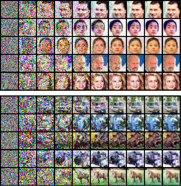
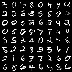
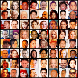
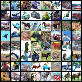
Image generation

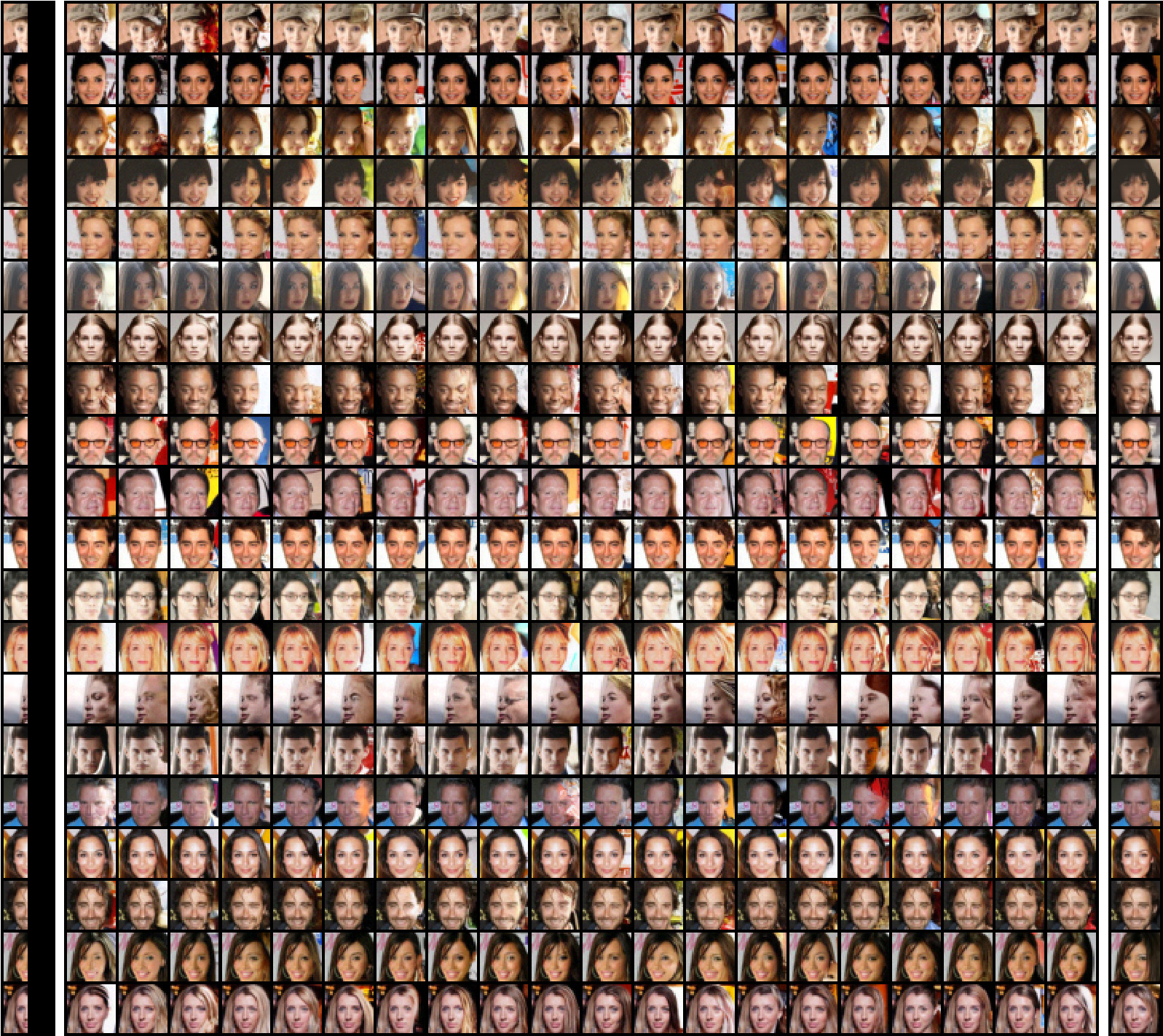
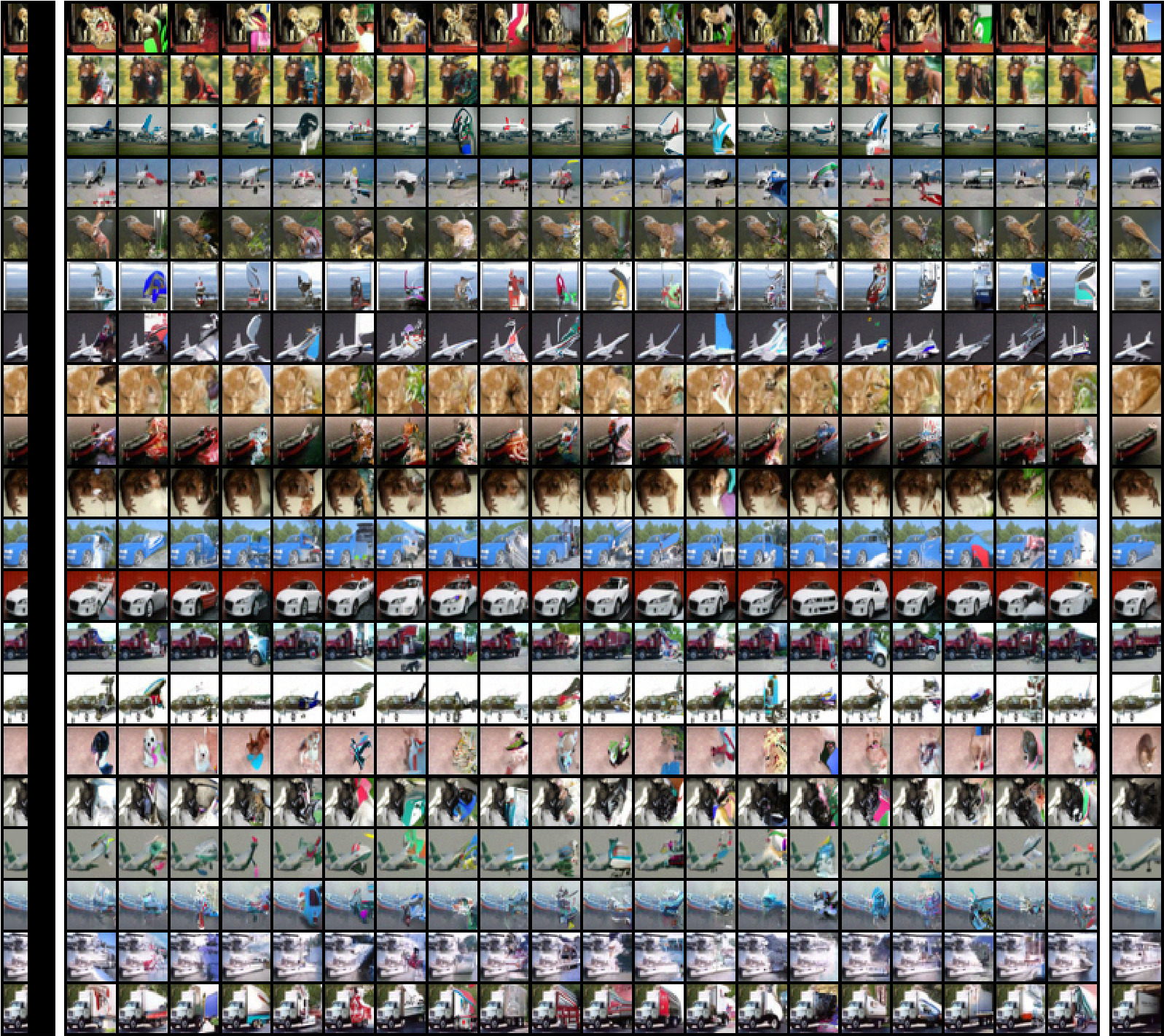
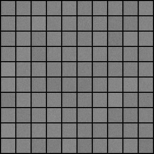
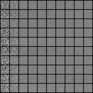
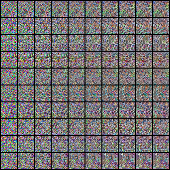
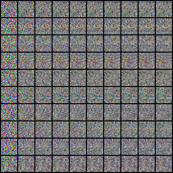
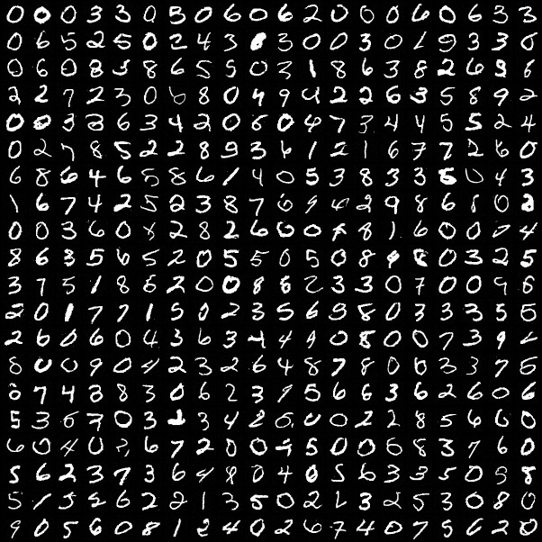
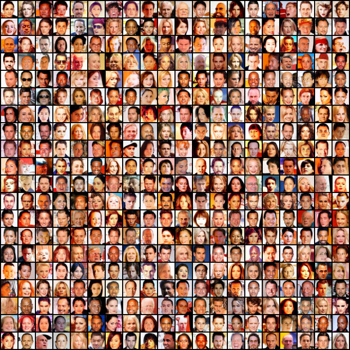
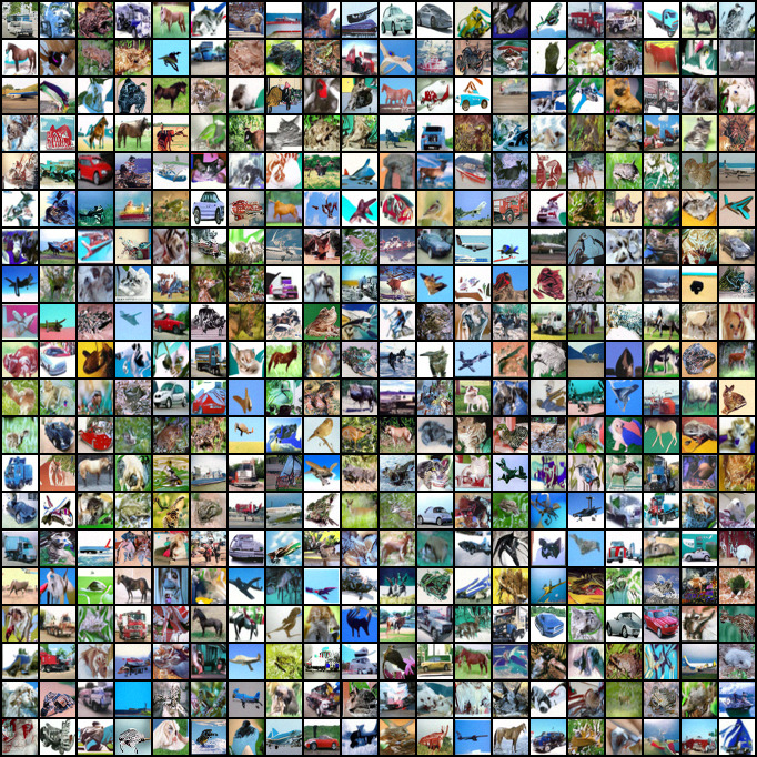
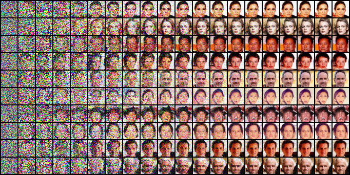
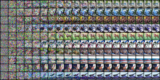
In Fig. 5, we show uncurated samples from annealed Langevin dynamics for MNIST, CelebA and CIFAR-10. As shown by the samples, our generated images have higher or comparable quality to those from modern likelihood-based models and GANs. To intuit the procedure of annealed Langevin dynamics, we provide intermediate samples in Fig. 4, where each row shows how samples evolve from pure random noise to high quality images. More samples from our approach can be found in Appendix C. We also show the nearest neighbors of generated images in the training dataset in Appendix C.2, in order to demonstrate that our model is not simply memorizing training images. To show it is important to learn a conditional score network jointly for many noise levels and use annealed Langevin dynamics, we compare against a baseline approach where we only consider one noise level $\{\sigma_{1}=0.01\}$ and use the vanilla Langevin dynamics sampling method. Although this small added noise helps circumvent the difficulty of the manifold hypothesis (as shown by Fig. 1, things will completely fail if no noise is added), it is not large enough to provide information on scores in regions of low data density. As a result, this baseline fails to generate reasonable images, as shown by samples in Appendix C.1.

For quantitative evaluation, we report inception [48] and FID [20] scores on CIFAR-10 in Tab. 1. As an unconditional model, we achieve the state-of-the-art inception score of 8.87, which is even better than most reported values for class-conditional generative models. Our FID score 25.32 on CIFAR-10 is also comparable to top existing models, such as SNGAN [36]. We omit scores on MNIST and CelebA as the scores on these two datasets are not widely reported, and different preprocessing (such as the center crop size of CelebA) can lead to numbers not directly comparable.

Figure 6: Image inpainting on CelebA (left) and CIFAR-10 (right). The leftmost column of each figure shows the occluded images, while the rightmost column shows the original images.

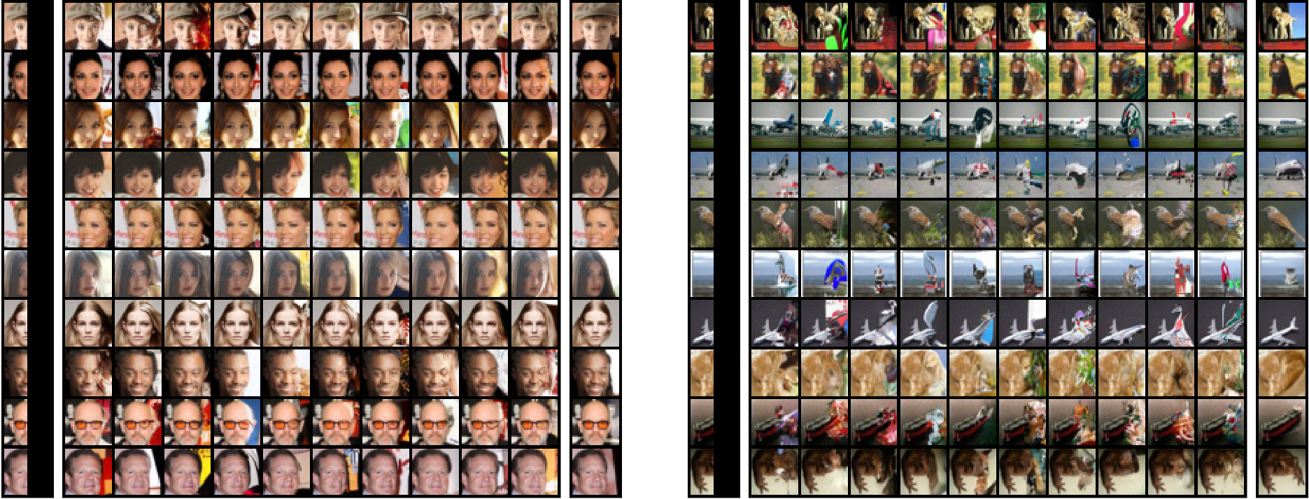
Image inpainting

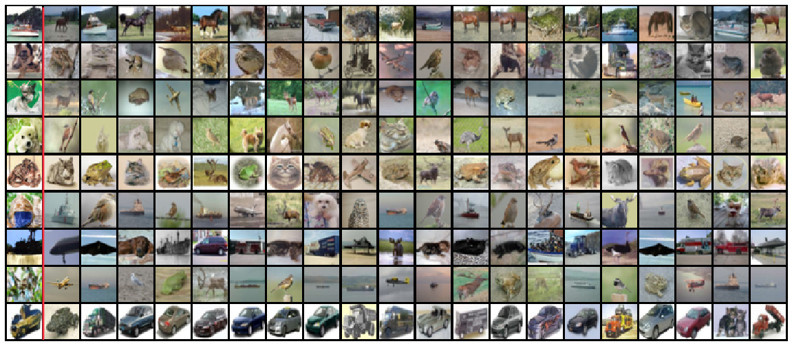
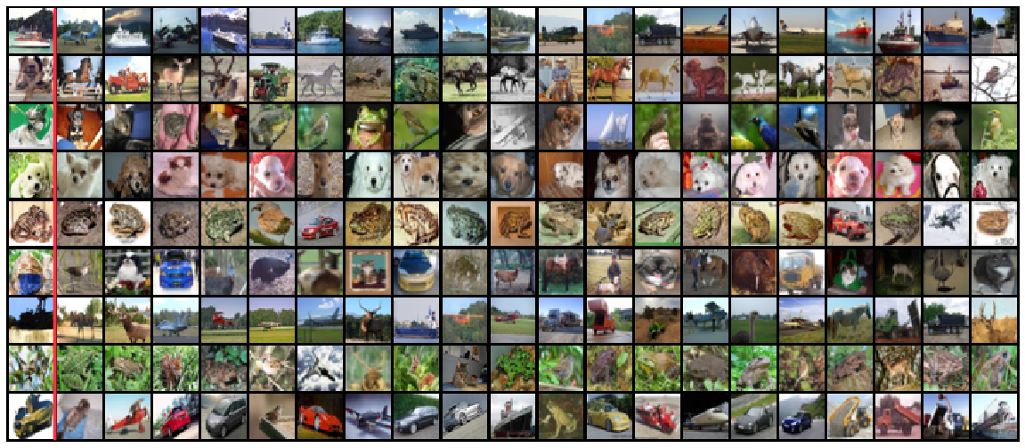
In Fig. 6, we demonstrate that our score networks learn generalizable and semantically meaningful image representations that allow it to produce diverse image inpaintings. Note that some previous models such as PixelCNN can only impute images in the raster scan order. In contrast, our method can naturally handle images with occlusions of arbitrary shapes by a simple modification of the annealed Langevin dynamics procedure (details in Appendix B.3). We provide more image inpainting results in Appendix C.5.

6 Related work

Our approach has some similarities with methods that learn the transition operator of a Markov chain for sample generation [4, 51, 5, 16, 52]. For example, generative stochastic networks (GSN [4, 1]) use denoising autoencoders to train a Markov chain whose equilibrium distribution matches the data distribution. Similarly, our method trains the score function used in Langevin dynamics to sample from the data distribution. However, GSN often starts the chain very close to a training data point, and therefore requires the chain to transition quickly between different modes. In contrast, our annealed Langevin dynamics are initialized from unstructured noise. Nonequilibrium Thermodynamics (NET [51]) used a prescribed diffusion process to slowly transform data into random noise, and then learned to reverse this procedure by training an inverse diffusion. However, NET is not very scalable because it requires the diffusion process to have very small steps, and needs to simulate chains with thousands of steps at training time.

Previous approaches such as Infusion Training (IT [5]) and Variational Walkback (VW [16]) also employed different noise levels/temperatures for training transition operators of a Markov chain. Both IT and VW (as well as NET) train their models by maximizing the evidence lower bound of a suitable marginal likelihood. In practice, they tend to produce blurry image samples, similar to variational autoencoders. In contrast, our objective is based on score matching instead of likelihood, and we can produce images comparable to GANs.

There are several structural differences that further distinguish our approach from previous methods discussed above. First, we do not need to sample from a Markov chain during training. In contrast, the walkback procedure of GSNs needs multiple runs of the chain to generate “negative samples”. Other methods including NET, IT, and VW also need to simulate a Markov chain for every input to compute the training loss. This difference makes our approach more efficient and scalable for training deep models. Secondly, our training and sampling methods are decoupled from each other. For score estimation, both sliced and denoising score matching can be used. For sampling, any method based on scores is applicable, including Langevin dynamics and (potentially) Hamiltonian Monte Carlo [38]. Our framework allows arbitrary combinations of score estimators and (gradient-based) sampling approaches, whereas most previous methods tie the model to a specific Markov chain. Finally, our approach can be used to train energy-based models (EBM) by using the gradient of an energy-based model as the score model. In contrast, it is unclear how previous methods that learn transition operators of Markov chains can be directly used for training EBMs.

Score matching was originally proposed for learning EBMs. However, many existing methods based on score matching are either not scalable [24] or fail to produce samples of comparable quality to VAEs or GANs [27, 49]. To obtain better performance on training deep energy-based models, some recent works have resorted to contrastive divergence [21], and propose to sample with Langevin dynamics for both training and testing [12, 39]. However, unlike our approach, contrastive divergence uses the computationally expensive procedure of Langevin dynamics as an inner loop during training. The idea of combining annealing with denoising score matching has also been investigated in previous work under different contexts. In [14, 7, 66], different annealing schedules on the noise for training denoising autoencoders are proposed. However, their work is on learning representations for improving the performance of classification, instead of generative modeling. The method of denoising score matching can also be derived from the perspective of Bayes least squares [43, 44], using techniques of Stein’s Unbiased Risk Estimator [35, 56].

7 Conclusion

We propose the framework of score-based generative modeling where we first estimate gradients of data densities via score matching, and then generate samples via Langevin dynamics. We analyze several challenges faced by a naïve application of this approach, and propose to tackle them by training Noise Conditional Score Networks (NCSN) and sampling with annealed Langevin dynamics. Our approach requires no adversarial training, no MCMC sampling during training, and no special model architectures. Experimentally, we show that our approach can generate high quality images that were previously only produced by the best likelihood-based models and GANs. We achieve the new state-of-the-art inception score on CIFAR-10, and an FID score comparable to SNGANs.

Acknowledgements

Toyota Research Institute ("TRI") provided funds to assist the authors with their research but this article solely reflects the opinions and conclusions of its authors and not TRI or any other Toyota entity. This research was also supported by NSF (#1651565, #1522054, #1733686), ONR (N00014-19-1-2145), AFOSR (FA9550-19-1-0024).

Appendix A Architectures

The architecture of our NCSNs used in the experiments has three important components: instance normalization, dilated convolutions and U-Net-type architectures. Below we give more background on them and discuss how we modified them to suit our purpose. For more comprehensive details and a reference implementation, we recommend the readers to check our publicly available code base. Our score networks are implemented in PyTorch. Code and checkpoints are available at https://github.com/ermongroup/ncsn.

A.1 Instance normalization

We use conditional instance normalization [13] so that $\mathbf{s}_{\boldsymbol{\theta}}(\mathbf{x},\sigma)$ takes account of $\sigma$ when predicting the scores. In conditional instance normalization, a different set of scales and biases is used for different $\sigma\in\{\sigma_{i}\}_{i=1}^{L}$. More specifically, suppose $\mathbf{x}$ is an input with $C$ feature maps. Let $\mu_{k}$ and $s_{k}$ denote the mean and standard deviation of the $k$-th feature map of $\mathbf{x}$, taken along the spatial axes. Conditional instance normalization is achieved by

$$\mathbf{z}_{k}=\gamma[i,k]\frac{\mathbf{x}_{k}-\mu_{k}}{s_{k}}+\beta[i,k],$$

where $\gamma\in\mathbb{R}^{L\times C}$ and $\beta\in\mathbb{R}^{L\times C}$ are learnable parameters, $k$ denotes the index of feature maps, and $i$ denotes the index of $\sigma$ in $\{\sigma_{i}\}_{i=1}^{L}$.

However, one downside of instance normalization is that it completely removes the information of $\mu_{k}$ for different feature maps. This can lead to shifted colors in the generated images. To fix this issue, we propose a simple modification to conditional instance normalization. First, we compute the mean and standard deviation of $\mu_{k}$’s and denote them as $m$ and $v$ respectively. Then, we add another learnable parameter $\alpha\in\mathbb{R}^{L\times C}$. The modified conditional instance normalization is defined as

$$\mathbf{z}_{k}=\gamma[i,k]\frac{\mathbf{x}_{k}-\mu_{k}}{s_{k}}+\beta[i,k]+\alpha[i,k]\frac{\mu_{k}-m}{v}.$$

We abbreviate this modification of conditional instance normalization as CondInstanceNorm++. In our architecture, we add CondInstanceNorm++ before every convolutional layer and pooling layer.

A.2 Dilated convolutions

Dilated convolutions can be used to increase the size of receptive field while maintaining the resolution of feature maps. It has been shown very effective in semantic segmentation because they preserve the location information better using feature maps of larger resolutions. In our architecture design of NCSNs, we use it to replace all the subsampling layers except the first one.

A.3 U-Net architecture

U-Net is an architecture with special skip connections. These skip connections help transfer lower level information in shallow layers to deeper layers of the network. Since the shallower layers often contain low level information such as location and shape, these skip connections help improve the result of semantic segmentation. For building $\mathbf{s}_{\boldsymbol{\theta}}(\mathbf{x},\sigma)$, we use the architecture of RefineNet [32], a modern variant of U-Net that also incorporates ResNet designs. We refer the readers to [32] for a detailed description of the RefineNet architecture.

In our experiments, we use a 4-cascaded RefineNet. We use pre-activation residual blocks. We remove all batch normalizations in the RefineNet architecture, and replace them with CondInstanceNorm++. We replace the max pooling layers in Refine Blocks with average pooling, as average pooling is reported to produce smoother images for image generation tasks such as style transfer. In addition, we also add CondInstanceNorm++ before each convolution and average pooling in the Refine Blocks, although no normalization is used in the original Refine Blocks. All activation functions are chosen to be ELU. As mentioned previously, we use dilated convolutions to replace the subsampling layers in residual blocks, except the first one. Following the common practice, we increase the dilation by a factor of 2 when proceeding to the next cascade. For CelebA and CIFAR-10 experiments, the number of filters for layers corresponding to the first cascade is 128, while the number of filters for other cascades are doubled. For MNIST experiments, the number of filters are halved.

Appendix B Additional experimental details

B.1 Toy experiments

For the results in Fig. 1, we train a ResNet with sliced score matching on CIFAR-10. We use pre-activation residual blocks, and the ResNet is structured as an auto-encoder, where the encoder contains 5 residual blocks and the decoder mirrors the architecture of the encoder. The number of filters for each residual block of the encoder part is respectively 32, 64, 64, 128 and 128. The 2nd and 4th residual block of the encoder subsamples the feature maps by a factor of two. We use ELU activations throughout the network. We train the network with 50000 iterations using Adam optimizer and a batch size of 128 and learning rate of 0.001. The experiment was run on one Titan XP GPU.

For the results in Fig. 2, we choose $p_{\text{data}}=\frac{1}{5}\mathcal{N}((-5,-5),I)+\frac{4}{5}\mathcal{N}((5,5),I)$. The score network is a 3-layer MLP with 128 hidden units and softplus activation functions. We train the score network with sliced score matching for 10000 iterations with Adam optimizer. The learning rate is 0.001, and the batch size is 128. The experiment was run on an Intel Core i7 GPU with 2.7GHz.

For the results in Fig. 3, we use the same toy distribution $p_{\text{data}}=\frac{1}{5}\mathcal{N}((-5,-5),I)+\frac{4}{5}\mathcal{N}((5,5),I)$. We generate 1280 samples for each subfigure of Fig. 3. The initial samples are all uniformly chosen in the square $[-8,8]\times[-8,8]$. For Langevin dynamics, we use $T=1000$ and $\epsilon=0.1$. For annealed Langevin dynamics, we use $T=100$, $L=10$ and $\epsilon=0.1$. We choose $\{\sigma_{i}\}_{i=1}^{L}$ to be a geometric progression, with $L=10$, $\sigma_{1}=20$ and $\sigma_{10}=1$. Both Langevin methods use the ground-truth data score for sampling. The experiment was run on an Intel Core i7 GPU with 2.7GHz.

B.2 Image generation

During training, we randomly flip the images in CelebA and CIFAR-10. All models are optimized by Adam with learning rate $0.001$ for a total of 200000 iterations. The batch size is fixed to 128. We save one checkpoint every 5000 iterations. For MNIST, we choose the last checkpoint at the 200000-th training iteration. For selecting our CIFAR-10 and CelebA models, we generate 1000 images for each checkpoint and choose the one with the smallest FID score computed on these 1000 images. Our image samples and results in Tab. 1 are from these checkpoints. Similar model selection procedures have been used in previous work, such as ProgressiveGAN [25].

The inception and FID scores are computed using the official code from OpenAI  [48] and TTUR [20] authors respectively. The architectures are described in Appendix A. When reporting the numbers in Tab. 1, we compute inception and FID scores based on a total of 50000 samples.

The baseline model uses the same score network. The only difference is that the score network is only conditioned on one noise level $\{\sigma_{1}=0.01\}$. When sampling using Langevin dynamics, we use $\epsilon=2\times 10^{-5}$ and $T=1000$.

The models on MNIST were run with one Titan XP GPU, while the models on CelebA and CIFAR-10 used two Titan XP GPUs.

B.3 Image inpainting

We use the following Alg. 2 for image inpainting.

Algorithm 2 Inpainting with annealed Langevin dynamics.

1:$\{\sigma_{i}\}_{i=1}^{L},\epsilon,T$ $\triangleright$ $\epsilon$ is smallest step size; $T$ is the number of iteration for each noise level.

2:$\mathbf{m},\mathbf{x}$ $\triangleright$ $\mathbf{m}$ is a mask to indicate regions not occluded; $\mathbf{x}$ is the given image.

3:Initialize $\tilde{\mathbf{x}}_{0}$

4:for $i\leftarrow 1$ to $L$ do

5:     $\alpha_{i}\leftarrow\epsilon\cdot\sigma_{i}^{2}/\sigma_{L}^{2}$ $\triangleright$ $\alpha_{i}$ is the step size.

6:     Draw $\tilde{\mathbf{z}}\sim\mathcal{N}(0,\sigma_{i}^{2})$

7:     $\mathbf{y}\leftarrow\mathbf{x}+\tilde{\mathbf{z}}$

8:     for $t\leftarrow 1$ to $T$ do

9:         Draw $\mathbf{z}_{t}\sim\mathcal{N}(0,I)$

10:         $\tilde{\mathbf{x}}_{t}\leftarrow\tilde{\mathbf{x}}_{t-1}+\dfrac{\alpha_{i}}{2}\mathbf{s}_{\boldsymbol{\theta}}(\tilde{\mathbf{x}}_{t-1},\sigma_{i})+\sqrt{\alpha_{i}}~{}\mathbf{z}_{t}$

11:         $\tilde{\mathbf{x}}_{t}\leftarrow\tilde{\mathbf{x}}_{t}\odot(1-\mathbf{m})+\mathbf{y}\odot\mathbf{m}$

12:     end for

13:     $\tilde{\mathbf{x}}_{0}\leftarrow\tilde{\mathbf{x}}_{T}$

14:end for

15:return $\tilde{\mathbf{x}}_{T}$

The hyperparameters are the same as those of the annealed Langevin dynamics used for image generation.

Appendix C Samples

C.1 Samples from the baseline models

(a) MNIST

(b) CelebA

(c) CIFAR-10

Figure 7: Uncurated samples on MNIST, CelebA, and CIFAR-10 datasets from the baseline model.

(a) MNIST

(b) CelebA

(c) CIFAR-10

Figure 8: Intermediate samples from Langevin dynamics for the baseline model.

C.2 Nearest neighbors

Figure 9: Nearest neighbors measured by the $\ell_{2}$ distance between images. Images on the left of the red vertical line are samples from NCSN. Images on the right are nearest neighbors in the training dataset.

Figure 10: Nearest neighbors measured by the $\ell_{2}$ distance in the feature space of an Inception V3 network pretrained on ImageNet. Images on the left of the red vertical line are samples from NCSN. Images on the right are nearest neighbors in the training dataset.

C.3 Extended samples

Figure 11: Extended MNIST samples

Figure 12: Extended CelebA samples

Figure 13: Extended CIFAR-10 samples

C.4 Extended intermediate samples from annealed Langevin dynamics

Figure 14: Extended intermediate samples from annealed Langevin dynamics for CelebA.

Figure 15: Extended intermediate samples from annealed Langevin dynamics for CelebA.

C.5 Extended image inpainting results

Figure 16: Extended image inpainting results for CelebA. The leftmost column of each figure shows the occluded images, while the rightmost column shows the original images.

Figure 17: Extended image inpainting results for CIFAR-10. The leftmost column of each figure shows the occluded images, while the rightmost column shows the original images.

References

- [1] G. Alain, Y. Bengio, L. Yao, J. Yosinski, E. Thibodeau-Laufer, S. Zhang, and P. Vincent. GSNs: generative stochastic networks. Information and Inference, 2016.
- [2] M. Arjovsky, S. Chintala, and L. Bottou. Wasserstein generative adversarial networks. In D. Precup and Y. W. Teh, editors, Proceedings of the 34th International Conference on Machine Learning, volume 70 of Proceedings of Machine Learning Research, pages 214–223, International Convention Centre, Sydney, Australia, 06–11 Aug 2017. PMLR.
- [3] M. Belkin and P. Niyogi. Laplacian eigenmaps for dimensionality reduction and data representation. Neural computation, 15(6):1373–1396, 2003.
- [4] Y. Bengio, L. Yao, G. Alain, and P. Vincent. Generalized denoising auto-encoders as generative models. In Advances in neural information processing systems, pages 899–907, 2013.
- [5] F. Bordes, S. Honari, and P. Vincent. Learning to generate samples from noise through infusion training. arXiv preprint arXiv:1703.06975, 2017.
- [6] A. Brock, J. Donahue, and K. Simonyan. Large scale GAN training for high fidelity natural image synthesis. In International Conference on Learning Representations, 2019.
- [7] B. Chandra and R. K. Sharma. Adaptive noise schedule for denoising autoencoder. In International conference on neural information processing, pages 535–542. Springer, 2014.
- [8] L.-C. Chen, G. Papandreou, I. Kokkinos, K. Murphy, and A. L. Yuille. Deeplab: Semantic image segmentation with deep convolutional nets, atrous convolution, and fully connected crfs. IEEE transactions on pattern analysis and machine intelligence, 40(4):834–848, 2017.
- [9] T. Chen, E. Fox, and C. Guestrin. Stochastic gradient hamiltonian monte carlo. In International conference on machine learning, pages 1683–1691, 2014.
- [10] Z. Dai, Z. Yang, F. Yang, W. W. Cohen, and R. R. Salakhutdinov. Good semi-supervised learning that requires a bad gan. In Advances in neural information processing systems, pages 6510–6520, 2017.
- [11] L. Dinh, D. Krueger, and Y. Bengio. Nice: Non-linear independent components estimation. arXiv preprint arXiv:1410.8516, 2014.
- [12] Y. Du and I. Mordatch. Implicit generation and generalization in energy-based models. arXiv preprint arXiv:1903.08689, 2019.
- [13] V. Dumoulin, J. Shlens, and M. Kudlur. A learned representation for artistic style. In International Conference on Learning Representations 2017, 2017.
- [14] K. J. Geras and C. Sutton. Scheduled denoising autoencoders. arXiv preprint arXiv:1406.3269, 2014.
- [15] I. Goodfellow, J. Pouget-Abadie, M. Mirza, B. Xu, D. Warde-Farley, S. Ozair, A. Courville, and Y. Bengio. Generative adversarial nets. In Advances in neural information processing systems, pages 2672–2680, 2014.
- [16] A. G. A. P. Goyal, N. R. Ke, S. Ganguli, and Y. Bengio. Variational walkback: Learning a transition operator as a stochastic recurrent net. In Advances in Neural Information Processing Systems, pages 4392–4402, 2017.
- [17] A. Graves. Generating sequences with recurrent neural networks. arXiv preprint arXiv:1308.0850, 2013.
- [18] I. Gulrajani, F. Ahmed, M. Arjovsky, V. Dumoulin, and A. C. Courville. Improved training of wasserstein gans. In Advances in Neural Information Processing Systems, pages 5767–5777, 2017.
- [19] M. Gutmann and A. Hyvärinen. Noise-contrastive estimation: A new estimation principle for unnormalized statistical models. In Proceedings of the Thirteenth International Conference on Artificial Intelligence and Statistics, pages 297–304, 2010.
- [20] M. Heusel, H. Ramsauer, T. Unterthiner, B. Nessler, and S. Hochreiter. Gans trained by a two time-scale update rule converge to a local nash equilibrium. In Advances in Neural Information Processing Systems, pages 6626–6637, 2017.
- [21] G. E. Hinton. Training products of experts by minimizing contrastive divergence. Neural computation, 14(8):1771–1800, 2002.
- [22] J. Ho and S. Ermon. Generative adversarial imitation learning. In Advances in Neural Information Processing Systems, pages 4565–4573, 2016.
- [23] X. Huang and S. Belongie. Arbitrary style transfer in real-time with adaptive instance normalization. In Proceedings of the IEEE International Conference on Computer Vision, pages 1501–1510, 2017.
- [24] A. Hyvärinen. Estimation of non-normalized statistical models by score matching. Journal of Machine Learning Research, 6(Apr):695–709, 2005.
- [25] T. Karras, T. Aila, S. Laine, and J. Lehtinen. Progressive growing of GANs for improved quality, stability, and variation. In International Conference on Learning Representations, 2018.
- [26] T. Karras, S. Laine, and T. Aila. A style-based generator architecture for generative adversarial networks. arXiv preprint arXiv:1812.04948, 2018.
- [27] D. Kingma and Y. LeCun. Regularized estimation of image statistics by score matching. In Advances in Neural Information Processing Systems 23: 24th Annual Conference on Neural Information Processing Systems 2010, NIPS 2010, 2010.
- [28] D. P. Kingma, S. Mohamed, D. J. Rezende, and M. Welling. Semi-supervised learning with deep generative models. In Advances in neural information processing systems, pages 3581–3589, 2014.
- [29] D. P. Kingma and M. Welling. Auto-encoding variational bayes. In ICLR, 2014.
- [30] S. Kirkpatrick, C. D. Gelatt, and M. P. Vecchi. Optimization by simulated annealing. SCIENCE, 220(4598):671–680, 1983.
- [31] A. Krizhevsky. Learning multiple layers of features from tiny images. Technical report, 2009.
- [32] G. Lin, A. Milan, C. Shen, and I. Reid. Refinenet: Multi-path refinement networks for high-resolution semantic segmentation. In Proceedings of the IEEE conference on computer vision and pattern recognition, pages 1925–1934, 2017.
- [33] Q. Liu, J. Lee, and M. Jordan. A kernelized stein discrepancy for goodness-of-fit tests. In International Conference on Machine Learning, pages 276–284, 2016.
- [34] Z. Liu, P. Luo, X. Wang, and X. Tang. Deep learning face attributes in the wild. In Proceedings of International Conference on Computer Vision (ICCV), 2015.
- [35] K. Miyasawa. An empirical bayes estimator of the mean of a normal population. Bull. Inst. Internat. Statist, 38(181-188):1–2, 1961.
- [36] T. Miyato, T. Kataoka, M. Koyama, and Y. Yoshida. Spectral normalization for generative adversarial networks. In International Conference on Learning Representations, 2018.
- [37] R. M. Neal. Annealed importance sampling. Statistics and computing, 11(2):125–139, 2001.
- [38] R. M. Neal. Mcmc using hamiltonian dynamics. arXiv preprint arXiv:1206.1901, 2012.
- [39] E. Nijkamp, M. Hill, T. Han, S.-C. Zhu, and Y. N. Wu. On the anatomy of mcmc-based maximum likelihood learning of energy-based models. arXiv preprint arXiv:1903.12370, 2019.
- [40] S. Nowozin, B. Cseke, and R. Tomioka. f-gan: Training generative neural samplers using variational divergence minimization. In Advances in neural information processing systems, pages 271–279, 2016.
- [41] G. Ostrovski, M. G. Bellemare, A. van den Oord, and R. Munos. Count-based exploration with neural density models. In Proceedings of the 34th International Conference on Machine Learning-Volume 70, pages 2721–2730. JMLR. org, 2017.
- [42] G. Ostrovski, W. Dabney, and R. Munos. Autoregressive quantile networks for generative modeling. In ICML, volume 80 of Proceedings of Machine Learning Research, pages 3933–3942. PMLR, 2018.
- [43] M. Raphan and E. P. Simoncelli. Learning to be bayesian without supervision. In Advances in neural information processing systems, pages 1145–1152, 2007.
- [44] M. Raphan and E. P. Simoncelli. Least squares estimation without priors or supervision. Neural computation, 23(2):374–420, 2011.
- [45] S. Ravuri, S. Mohamed, M. Rosca, and O. Vinyals. Learning implicit generative models with the method of learned moments. In J. Dy and A. Krause, editors, Proceedings of the 35th International Conference on Machine Learning, volume 80 of Proceedings of Machine Learning Research, pages 4314–4323, Stockholmsmässan, Stockholm Sweden, 10–15 Jul 2018. PMLR.
- [46] O. Ronneberger, P.Fischer, and T. Brox. U-net: Convolutional networks for biomedical image segmentation. In Medical Image Computing and Computer-Assisted Intervention (MICCAI), volume 9351 of LNCS, pages 234–241. Springer, 2015. (available on arXiv:1505.04597 [cs.CV]).
- [47] S. T. Roweis and L. K. Saul. Nonlinear dimensionality reduction by locally linear embedding. science, 290(5500):2323–2326, 2000.
- [48] T. Salimans, I. Goodfellow, W. Zaremba, V. Cheung, A. Radford, and X. Chen. Improved techniques for training gans. In Advances in neural information processing systems, pages 2234–2242, 2016.
- [49] S. Saremi, A. Mehrjou, B. Schölkopf, and A. Hyvärinen. Deep energy estimator networks. arXiv preprint arXiv:1805.08306, 2018.
- [50] J. Sohl-Dickstein, P. Battaglino, and M. R. DeWeese. Minimum probability flow learning. arXiv preprint arXiv:0906.4779, 2009.
- [51] J. Sohl-Dickstein, E. Weiss, N. Maheswaranathan, and S. Ganguli. Deep unsupervised learning using nonequilibrium thermodynamics. In International Conference on Machine Learning, pages 2256–2265, 2015.
- [52] J. Song, S. Zhao, and S. Ermon. A-nice-mc: Adversarial training for mcmc. In Advances in Neural Information Processing Systems, pages 5140–5150, 2017.
- [53] Y. Song, S. Garg, J. Shi, and S. Ermon. Sliced score matching: A scalable approach to density and score estimation. In Proceedings of the Thirty-Fifth Conference on Uncertainty in Artificial Intelligence, UAI 2019, Tel Aviv, Israel, July 22-25, 2019, page 204, 2019.
- [54] Y. Song, T. Kim, S. Nowozin, S. Ermon, and N. Kushman. Pixeldefend: Leveraging generative models to understand and defend against adversarial examples. In International Conference on Learning Representations, 2018.
- [55] B. K. Sriperumbudur, K. Fukumizu, A. Gretton, B. Schölkopf, and G. R. Lanckriet. On integral probability metrics,phi-divergences and binary classification. arXiv preprint arXiv:0901.2698, 2009.
- [56] C. M. Stein. Estimation of the mean of a multivariate normal distribution. The annals of Statistics, pages 1135–1151, 1981.
- [57] D. Ulyanov, A. Vedaldi, and V. Lempitsky. Instance normalization: The missing ingredient for fast stylization. arXiv preprint arXiv:1607.08022, 2016.
- [58] A. van den Oord, S. Dieleman, H. Zen, K. Simonyan, O. Vinyals, A. Graves, N. Kalchbrenner, A. Senior, and K. Kavukcuoglu. Wavenet: A generative model for raw audio. In Arxiv, 2016.
- [59] A. Van den Oord, N. Kalchbrenner, L. Espeholt, O. Vinyals, A. Graves, et al. Conditional image generation with pixelcnn decoders. In Advances in neural information processing systems, pages 4790–4798, 2016.
- [60] A. Van Den Oord, N. Kalchbrenner, and K. Kavukcuoglu. Pixel recurrent neural networks. In Proceedings of the 33rd International Conference on International Conference on Machine Learning - Volume 48, ICML’16, pages 1747–1756. JMLR.org, 2016.
- [61] P. Vincent. A connection between score matching and denoising autoencoders. Neural computation, 23(7):1661–1674, 2011.
- [62] M. Welling and Y. W. Teh. Bayesian learning via stochastic gradient langevin dynamics. In Proceedings of the 28th international conference on machine learning (ICML-11), pages 681–688, 2011.
- [63] L. Wenliang, D. Sutherland, H. Strathmann, and A. Gretton. Learning deep kernels for exponential family densities. In International Conference on Machine Learning, pages 6737–6746, 2019.
- [64] F. Yu and V. Koltun. Multi-scale context aggregation by dilated convolutions. In International Conference on Learning Representations (ICLR), 2016.
- [65] F. Yu, V. Koltun, and T. Funkhouser. Dilated residual networks. In Computer Vision and Pattern Recognition (CVPR), 2017.
- [66] Q. Zhang and L. Zhang. Convolutional adaptive denoising autoencoders for hierarchical feature extraction. Frontiers of Computer Science, 12(6):1140–1148, 2018.