MLR (Memory, Learning and Recognition): A General Cognitive Model - applied to Intelligent Robots and Systems Control

Abstract

This paper introduces a new perspective of intelligent robots and systems control. The presented and proposed cognitive model: Memory, Learning and Recognition (MLR), is an effort to bridge the gap between Robotics, AI, Cognitive Science, and Neuroscience. The currently existing gap prevents us from integrating the current advancement and achievements of these four research fields which are actively trying to define intelligence in either application-based way or in generic way.

This cognitive model defines intelligence more specifically, parametrically and detailed. The proposed MLR model helps us create a general control model for robots and systems independent of their application domains and platforms since it is mainly based on the dataset provided for robots and systems controls.

This paper is mainly proposing and introducing this concept and trying to prove this concept in a small scale, firstly through experimentation. The proposed concept is also applicable to other different platforms in real-time as well as in simulation.

I Introduction

Intelligent control of robots and systems have been at the center of attention for decades since Robotics is a very useful and applicable field of research in human life. After DARPA 2005 [1, 2, 3], there have been significant investments into Probabilistic Robotics [4] (i.e. the usage of learning for robot control) and more specifically, in Autonomous Navigation.

Since then, we have also seen much industrial inclination toward applying this technology to their own products to create more intelligent machines such as Google self-driving cars. The main drawback, however, has always been a lack of common intelligent architecture or a lack of a concrete and applicable definition of intelligence which should somehow explain how it is possible to create an intelligent system.

Although there has been an enormous amount of financial investment with many attempts to define intelligence from different fields of research, none of them can actually explain intelligence (human intelligence specifically) in a way that it can be applicable to other fields of research, thus connecting all, i.e. there is a lack of an operational definition.

The current advancements in machine learning known as Deep Learning [5] has brought much hope and excitement about AI general applications and perhaps this is the right way to approach intelligence and its definition [6]. An interesting review paper presents the complete historical trend of the deep learning approach in Neural Networks [7].

Another recent excitement in AI was brought by the Deep Reinforcement Learning method proposed by [8] which is presenting a Deep Learning Approach in Atari games which is also a very simple and primitive simulated environment and robots (so- called agent in the paper) for testing the control efficiency of the deep learning approach.

The latter proposed approach claims to outperform human-level control of the simulated agent in the simulated environment of the Atari games; this is a very promising step forward toward understanding the true nature of intelligence and intelligent control of robots. The latter approach, DQN, has triggered some researchers to look into the new theory of Learn-See-Act instead of the previous Sense-Plan-Act [9] and [10].

II MLR (Memory, Learning and Recognition)

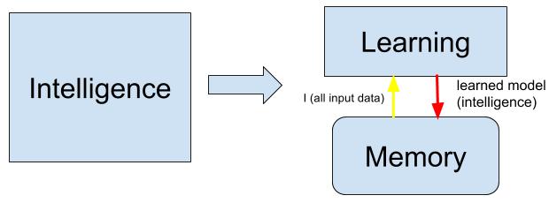
The proposed generic cognitive model is basically suggesting three main components for intelligent control: Memory, Learning and Recognition. These three components can also be categorized into three: Cognition (done by Recognition), knowledge (stored in Memory) and Intelligence (produced by learning) (please be advised that this categorization is proposed by this paper). Intelligence includes a combination of Memory and Leaning. For better understanding of the proposed model, the complete intelligent robot control architecture is illustrated in figure  1.

Figure 1: (left)The robot control architecture with four layers is presented, (right) Inside the first two layers are also shown.

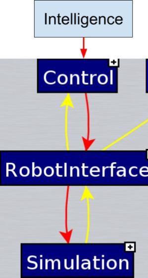
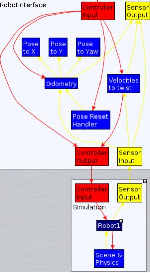
The left figure in 1 is showing that a complete intelligent robot and systems control architecture has four main layers; The first two layers are shown in more details in the right figure in  1.

As you can see the first two layers are preparing the robot to be able to deliver the sensor data to control module and also be able to receive the controlling commands from the control module in the third layer. It is important to know that our proposed cognitive model (MLR) is focusing only on the last and highest two layers, which defines intelligent control.

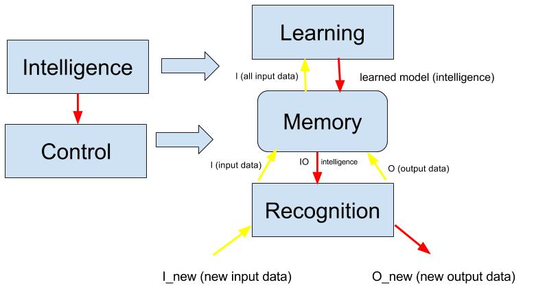
The first two layers are provided and illustrated along with the last and highest two layers to give you an overview of how our complete robot control architecture looks like and also how many layers are needed in either real or simulated robot in order to create a complete intelligent robot control. Figure 2 gives an overview of what is proposed in this paper as the cognitive model.

Figure 2: The main proposed conceptual cognitive model of intelligent control introduced as MLR

.

Based on this model, the control module equals to memory and recognition but the intelligence module is composed of memory and learning. The interesting thing about this model is that these two processes are done completely independently and can be performed on different computers and processors. In figures 3 and 4, you can see the model in more detail and as two completely independent processes.

Figure 3: The separate control module.

Figure 4: The separate intelligence module.

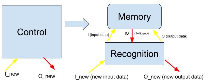
After Looking at the overall MLR architecture (the proposed cognitive model for intelligent control), now we will get into more detail on each one and how they work together.

II-A Memory

Memory is creating the data space and storage needed for writing data and reading data. Based on the memory limit and therefore our database limit, we can conclude that the intelligence created using the learning module and by learning the stored data in memory can not be beyond the limits of our input and output data stored in our memory. Basically, memory is giving us the database and based on the database, we can begin to create our own data space using learning. It is also very important to know that memorizing and remembering things play an important role in human intelligence and so the same may apply for robots and intelligent systems as well. In the proposed concept, we will start with writing Input Output $IO$ data to our memory (or the Hard disk of the computer).

$$IO=\left\{IO_{1},.............,IO_{t}\right\}$$

These input output data are sampled throughout time and are generally Sensor Output $I$ and Controller Input $O$ as shown in Ò(1). Parameter $t$ is the time index in which the data samples were acquired and recorded into memory.

The recorded $IO$ database in the memory is completely based on the manual controlling of the robot. Therefore, it is highly suggested to create Input-based Output, meaning the Sensor-based control data which is going to be used later by the robot itself for intelligent control.

II-B Learning

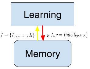
Having written and prepared the $IO$ database, we will use all the input data I for learning. Learning, in our work, is analyzing the input data space, decomposing data eigenvalues for creating input data eigenspace finally. But the main idea in learning is usually creating the Data Space in the first place. Data Space is also known as Data Feature Space or Feature Space. In order to create the feature space, We need to read all the input data from the memory as mentioned in Ò(2) and create a matrix of all input data vectors all at once.

$$I=\left\{I_{1},....,I_{t}\right\}$$

Once we have the matrix $I$, we mathematically have created the input data feature space. This matrix is a Column-Major matrix meaning that the number of columns are indicating the number of input data samples and the number of rows are indicating the number of input data dimensions.

Using PCA helps us create the data feature eigen space which is basically composed of the principle components. Principle components are also known as eigen values and eigen vectors of $I$ (Input Data Matrix). In order to do PCA, First of all we have to calculate $\mu$ (the mean) of $I$ as Òequation (3):

$$\mu=\frac{\sum_{1}^{t}I_{i}}{t}$$

Given $\mu$, we will start translating all the input vectors to the origin as Òequation (4):

$$I-\mu=\left\{I_{1}-\mu,....,I_{t}-\mu\right\}$$

$$I-\mu=\varphi,\ I_{1}-\mu=\varphi_{1},........,\ I_{t}-\mu=\varphi_{t}$$

$$\varphi=\left\{\varphi_{1},.......,\varphi_{t}\right\}$$

Once we have all $\varphi$, now we can start the principle component analysis (PCA) or eigenvalue decomposition as shown in  4 and mentioned in following Òequation (5):

$$A\cdot\nu=\lambda\cdot\nu\Rightarrow A=\nu\cdot\lambda\cdot\nu^{t}$$

Using eigenvalue decomposition, we can measure eigenvalues $\lambda$ and eigenvectors $\nu$. Also we should not forget that, according to Singular Value Decomposition (SVD) Òequation (5) and (6),

$$\varphi=\nu\cdot\Lambda\cdot\upsilon^{t}\Rightarrow\lambda=\Lambda^{2}$$

$$\varphi\cdotp\varphi^{t}=(\nu\cdot\Lambda\cdot\upsilon^{t})\cdotp(\nu\cdot\Lambda\cdot\upsilon^{t})^{t}=\nu\cdot\Lambda^{2}\cdot\nu^{t}$$

Therefore using the equations above Òequation (5) and (6), singular values $\Lambda$ can be measured using eigenvalues $\lambda$ which will help us in scaling that will be used later for recognition purposes  II-C. Having calculated $\mu$, $\Lambda$, $\nu$, we write them back into the memory. Basically the learning module reads the recorded input data from memory $I$ and generates the learned eigenspace information such as: $\mu$, $\Lambda$, $\nu$ which can be used to reduce the data dimensionality considerably to the handful of principle components. In figure  5, the input and the output of the learning module are specifically shown in reading $I$ from memory and writing $\mu$, $\Lambda$, $\nu$ back into the memory.

Figure 5: The input and output of the learning module (data flow).

II-C Recognition

Having learned the input data as discussed in previous section II-B, this module read the $IO$ recorded data both from sensors and controllers along with $\mu,\Lambda,\nu$ (learned principle components) as shown in figure  6.

Figure 6: The input and output of recognition module (data flow).

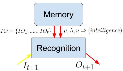
Once we read all the recorded data from the memory with their time index $IO_{t}$, we can start comparing the new input data $I_{t+1}$ with our learned input data in our database $I$. This comparison $I_{t+1}$ vs $I={I_{1},......,I_{t}}$ should be done intelligently meaning using the principle components ($\mu,\Lambda,\nu$) (or intelligence parameters). Basically in recognition, we are comparing $I_{t+1}$ with every single one of the input data in $I$ based on four different metrics in order to find the most similar and the least different existing recorded input data in our learned database.

Once we read all the recorded data from the memory with their time index $IO_{t}$, we can start comparing the new input data $I_{t+1}$ with our learned input data in our database $I$. This comparison $I_{t+1}$ vs $I={I_{1},......,I_{t}}$ should be done intelligently meaning using the principle components ($\mu,\Lambda,\nu$) (or intelligence parameters). Basically in recognition, we are comparing $I_{t+1}$ with every single one of the input data in $I$ based on four different metrics in order to find the most similar and the least different existing recorded input data in our learned database. In order to compare them, at first we need to project them onto the learned eigen space using $\mu,\Lambda,\nu$ as follows:

$$\varphi_{t+1}=I_{t+1}-\mu,\ \varphi=\left\{\varphi_{1},.......,\varphi_{t}\right\}$$

It is also important to know that the resulting number of principle components in maximum can be equal to the number of data samples $t$ but since we want to reduce the dimensionality of our data in a way that we can still accurately enough be able to reconstruct them, therefore $\nu=\left\{\nu_{1},........,\nu_{n}\right\}$, meaning that we only keep $n$ number of principle components ($\frac{n}{t}$ percentage of kept eigenvectors).

In Òequation (7), $n$ is indicating the number of principle components which is also considerably reduced compared to the initial number of input data dimensions.

$$\omega_{\varphi_{1}}=\nu\cdot\varphi_{1},......................,\omega_{\varphi_{t}}=\nu\cdot\varphi_{t}$$

$$\omega_{\varphi_{t+1}}=\nu\cdot\varphi_{t+1}$$

In Ò(8) and Ò(9), both new input data $I_{t+1}$ and the recorded input data in memory $I$ are projected to the learned eigenspace and can be reconstructed as shown in Òequation (10):

$$\varphi_{t+1}=\omega_{\varphi_{t+1}}\cdot\nu$$

When you can completely reconstruct all the recorded input data $I$ and the new one $I_{t+1}$, this means that we can easily compare them using their new projected values $\omega_{\varphi}$ vs $\omega_{\varphi_{t+1}}$ in the eigen space based on their principle components $\Lambda\nu=\left\{\Lambda_{1}\nu_{1},.................,\Lambda_{n}\nu_{n}\right\}$ based on four metrics as follows:

II-C1 Minimum Squared Difference

This metric is based on minimum distance between two vectors in the eigenspace as shown in Òequation (11). This metric is also known as Min Square Error and the min is 0 which means that the two vectors have no difference in this space and the max can be any value.

$$\left|\omega_{\varphi_{t+1}}-\omega_{\varphi_{1}}\right|,...................................,\left|\omega_{\varphi_{t+1}}-\omega_{\varphi_{t}}\right|$$

II-C2 Scaled Minimum Squared Difference

Minimum scaled difference is also based on minimum distance but it also applies the importance of every single principle components and since $\Lambda$ is basically $\omega_{max}$ on each component $\nu$, that is why using $\Lambda$ for scaling might really make the comparison more fair and more accurate (at least theoretically) between two vectors in the space as shown in Òequation (12).

$$\left\{\left|\frac{\omega_{\varphi_{t+1}}}{\Lambda}-\frac{\omega_{\varphi_{1}}}{\Lambda}\right|,........,\left|\frac{\omega_{\varphi_{t+1}}}{\Lambda}-\frac{\omega_{\varphi_{t}}}{\Lambda}\right|\right\}$$

II-C3 Maximum Normalized Cross Similarity

This metric is mainly measuring the angle between two vectors in the space and since the smaller the angle is, the more similar these two vectors are. This metric is also known as Normalized Cross Correlation which is basically the dot product or inner product of two vectors in the space as shown in Òequation (13) as follows:

$$\left\{\frac{\omega_{\varphi_{t+1}}}{\left|\omega_{\varphi_{t+1}}\right|}\cdot\frac{\omega_{\varphi_{1}}}{\left|\omega_{\varphi_{1}}\right|},...................,\frac{\omega_{\varphi_{t+1}}}{\left|\omega_{\varphi_{t+1}}\right|}\cdot\frac{\omega_{\varphi_{t}}}{\left|\omega_{\varphi_{t}}\right|}\right\}$$

The result of this metric is always $0\leq cos\angle\leq 1$ which makes it work more like a probability measurement.

II-C4 Scaled Maximum Cross Similarity

This metric is also mainly based on previous metric with two main differences:

• it is not normalized

• it is scaled using $Lamda$ with completely the same scaled minimum squared difference.

As you can see it in Òequation (14) as follows:

$$\left\{\frac{\omega_{\varphi_{t+1}}}{\Lambda}\cdot\frac{\omega_{\varphi_{1}}}{\Lambda},.....................,\frac{\omega_{\varphi_{t+1}}}{\Lambda}\cdot\frac{\omega_{\varphi_{t}}}{\Lambda}\right\}$$

Using all four metrics, we can almost precisely find the most similar and least different input data among $I=\left\{I_{1},......................,I_{t}\right\}$ to the new input data $I_{t+1}$ and once it is found, we can use its index $t$ and we can use its corresponding recorded output $IO=\left\{IO_{1},......................,IO_{t}\right\}$ as the new output $O_{t+1}$ for the new input data $I_{t+1}$.

III Experimental results

In order to speed up the implementation of the proposed MLR model, we decided to use the simulation. The simulated environment and simulated robot is the default, well-maintained and well-documented project in Finroc [12]. For the experimental setup, we are using Linux kernel in Ubuntu 14.04 (64 bit) and also as explained above, Finroc is our framework which is using its own simulation environment known as SimVis3D. The current available open-source project in Finroc is called Forklift and it has been used as the simulated experimental platform for testing the performance of our MLR model as follows: We chose our experimental setup in a way that it can show the exact role of each module in it and how they are working together.

III-A Recording the dataset into memory

The memory is very important module in the proposed MLR model since we have to start managing our memory in our experiments at first by writing sensor data into memory (will be later used as $I$). These sensor data are specifically camera images (the highest possible image resolution in simulation $900\times 700$ size and in $RGB$ scale), distance data and localization data. In this experiment, we decided to use only the camera images to show the power of the MLR model in dealing with high-dimensional input data and also for more clear understanding of the performance of the model in generating the controlling commands to the robot.

Also, we should write the controlling data $O$ at the same time with sensor data (controller data are generated initially by the data recorder and the person who is manually controlling the robot to record the data). These controlling commands are $O$ which will be recorded along with $I$ at the same time and gives us $IO$ dataset in the memory. The writing and reading data from memory has been illustrated before in figures  II-B,  II-A and  II-C.

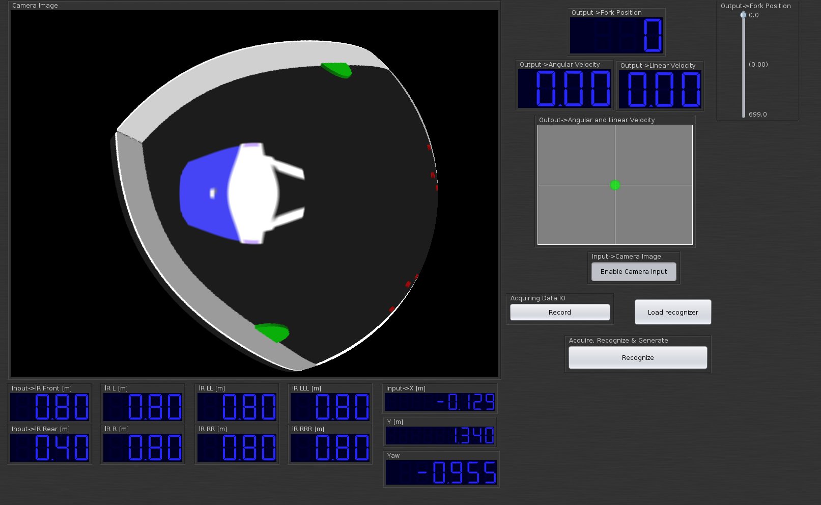
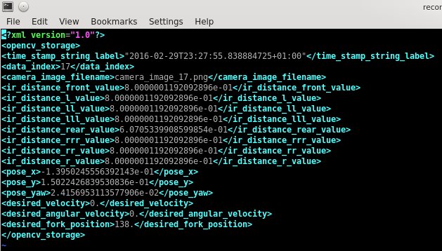
Using the Finroc GUI (Known as FinGUI), we can manually control the robot using joystick to explore the default simulated environment as shown in figure 7. At every specific date and specific length of time (or duration of time) in that date, we record only one dataset $IO=\left\{IO_{1},.................,IO_{t}\right\}$. The date of recording will be used as the directory in which all the data recorded will be written to and during recording, one index will be assigned to all of the data. The date of recording and the index of recorded data both are stored in an XML file shown in figure 8.

As you can see in this figure, the first row is time stamp label string which is the exact date of data recording accuracy. The second row is data index which is assigned to the recorded data during the recording to keep corresponding input and output data together. Data index also depends on the duration of recording the data as well. In this experiment, we had two different recordings which means two different time stamps or two complete different datasets. Each one of these recordings took about 10 minutes and we were recording at the speed on 1 data per second.

This means we have generated $1\times 10\times 60=600$ indexes of data in each recording or $IO={IO_{1},..........,IO_{600}}$. Therefore, in one recording we have a total of 600 camera images, with resolution of $900\times 700$ size and in $RGB$ scale recorded in our memory. These camera images will be used for learning and also for recognition. In XML file 8, the third row is also the name of the camera image and this image is stored in the same folder as the XML file is stored. The name of the folder (or the parent folder) is the same as the time stamp label which is the date of recording.

Also in XML file 8, after the camera image, there are distance data value which are more specifically 8 infra-red distance data values and localization data is also place after distance values composed of pose $X,Yand\ Yaw$. After localization data, there are controlling data value generated at the same time as these sensor data values. Controller value are desired linear velocity and angular velocity of the robot and also the position robot’s fork.

As you can see OpenCV [11] cv::FileStorage framework has been used for storing data into the memory. Also boost filesystem library [13] is used to search for files and store their paths so that it is possible to read the files from directory based on the XML file 8.

It is also important to notice that sensor data and controller data depends on the person who is manually controlling the robot and recording the data. Finally these recorded data create the robot intelligence which means that it is highly dependent on the data recorder intelligence.

In figure 7, the GUI for manually controlling the simulated robot and recording the data are shown along with the controller values on top of joystick and the distance value and localization values and camera image at the left side of the joystick. At right side of the joystick you can also see the fork position slider to manipulate the objects and obstacles in the environment.

Figure 7: A snapshot taken from GUI used to manually control the robot and record the $IO$ dataset.

Figure 8: The XML format in which the recorded data are converted to along with their labels and directory for better and accurate recognition.

III-B Learning the recorded dataset

Having recorded the data in the memory with labels including date of recording and the index of the recorded, now the learning process has begun. The tricky part here is to choose a threshold for the number of eigenvalues and the maximum number of eigenvalues to keep without hurting the accuracy of the work and also it is going to be very slow during the recognition process.

In this experiment, we are only using the camera images with highest possible resolution in Finroc simulation framework SimVis3D in order to prove the concept in handling a very large dimensional input data. Having read the file path of each camera images, we store them first into OpenCV Matrix and then we push them one by one to the vector. Basically each Matrix is the image data structure used in OpenCV [11] and the vector is the standard library vector class which is very efficient as data container class.

Once all the camera images are read and collected, we convert them all intro gray scale since they are all in RGB format. Therefore, we have to change them all from RGB (3-channel) to grayscale (1-channel) and also make sure that they are normalized meaning the pixel values are between 0-255. I call this process scaling the data and it is mainly composed of converting RGB to Gray scale and normalizing the data to 0-255.

Having scaled the data, now we should vectorize all of our images or in simpler way we should change all the images into one column image. In result, we change vector to only one Mat in whose each column there is only one image. Images are stored as Column Data. This Matrix (Mat) is called $I={I_{1},........,I_{t}}$. In this case $t=600$ as explained in the process of recording dataset into memory III-A. Having created $I$ all the input data matrix (images in this case), now data space can be created and learned using PCA engine in OpenCV [11]. There are plenty of implementations of PCA, SVD and Eigen Value Decomposition (EVD) which might be implemented in different ways.

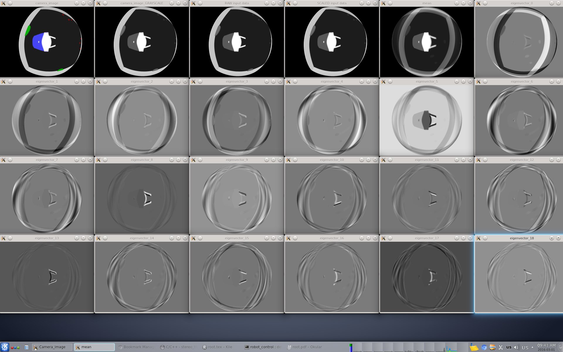
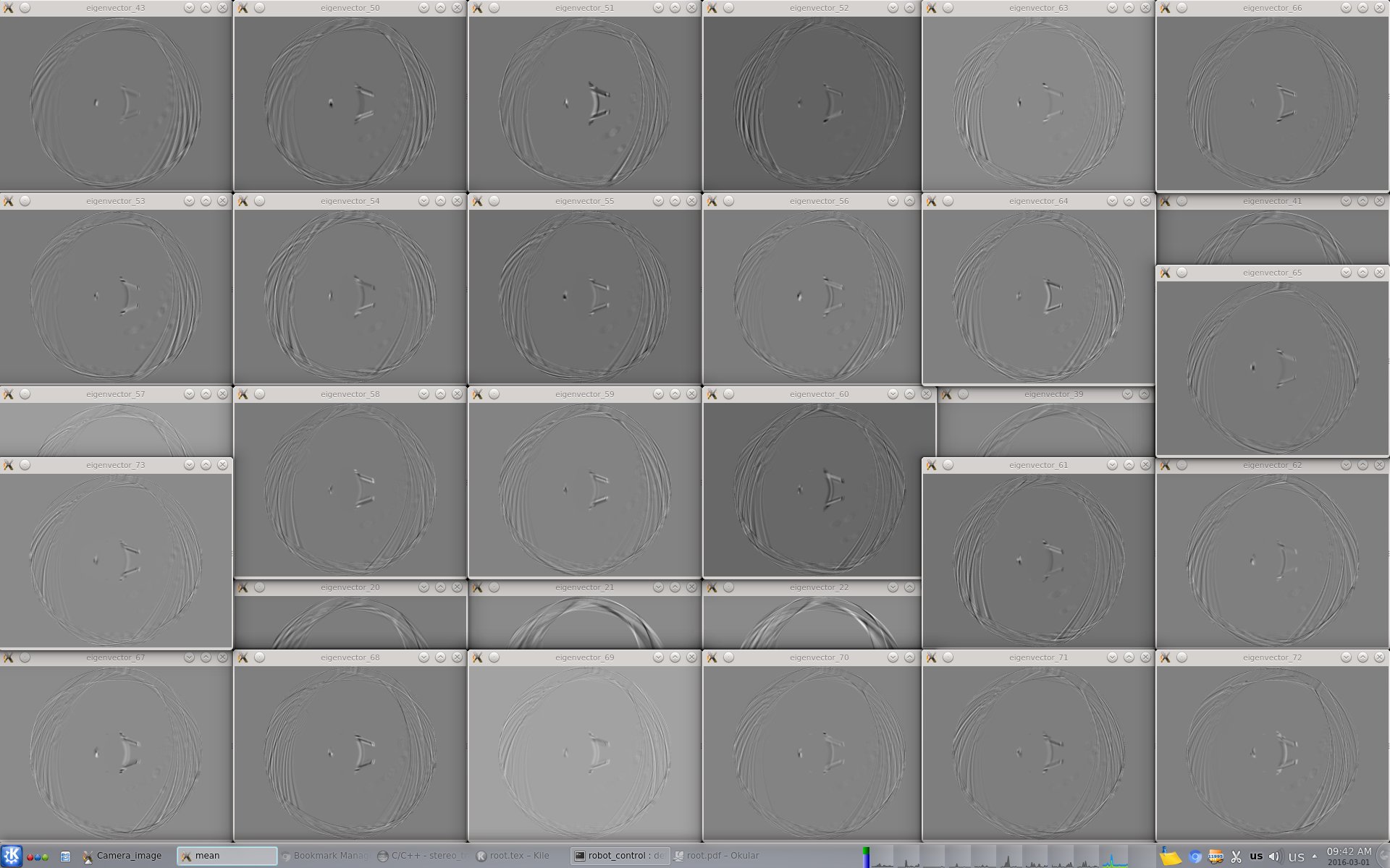
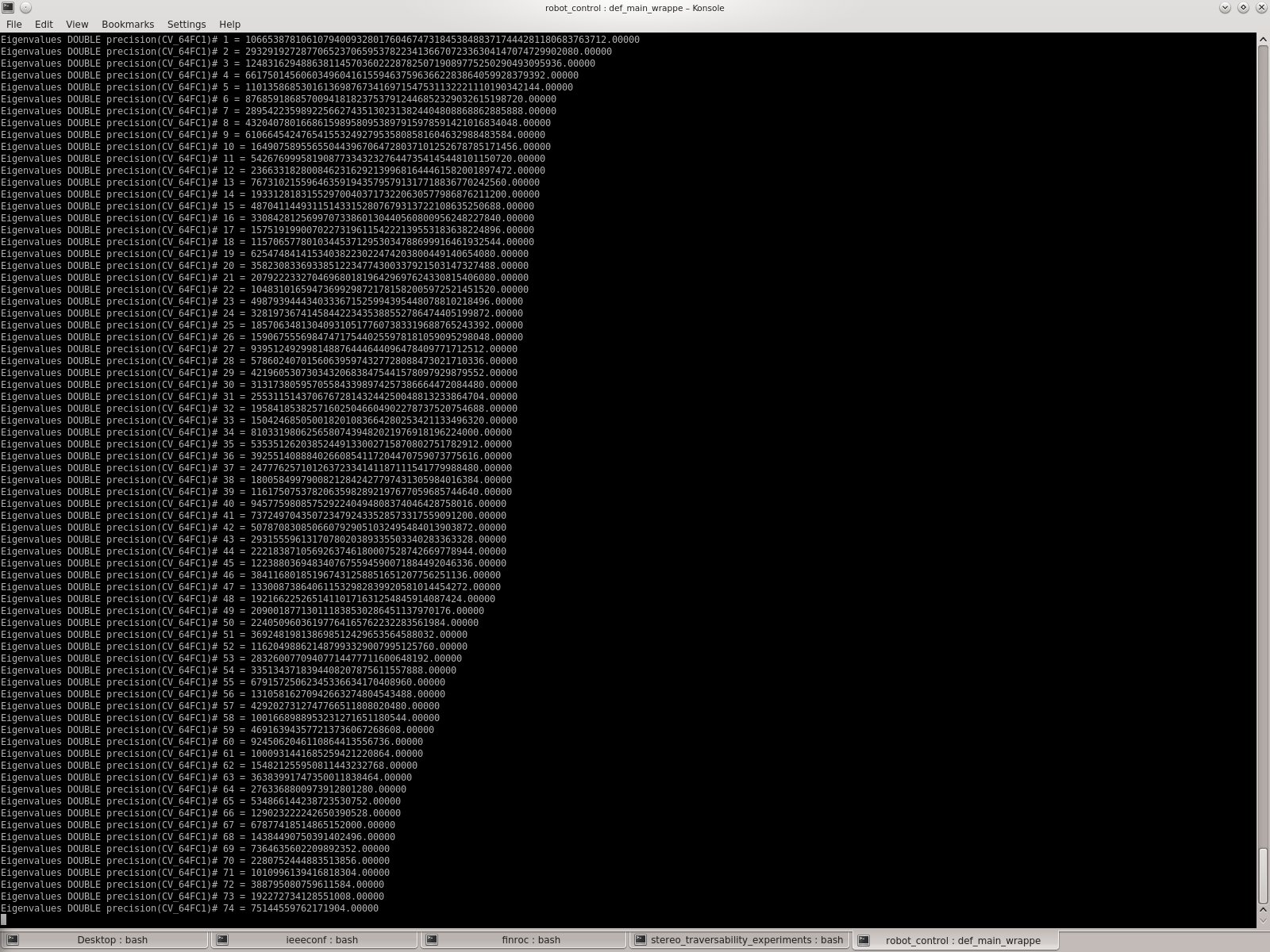
This would be an interesting research idea to also compare their results all together and see if their results are the same or not since some of them like OpenCV PCA engine is supporting the float precision value and some other implementations such as Matlab and Python are generating the results with Double precision. Using the PCA engine, we can calculate the mean $\mu,\Lambda and\nu$ which are all shown in figure 9 in order of the eigenvalues which are also shown in figure 11 and also the eigenvectors corresponds to the smaller eigenvalues are also shown in figure 10 only to give you a better idea how the eigenvectors changing in order of their corresponding eigenvalues.

In our experiment, we choose the first five principle components for data projections. This means that we just reduce the dimensionality of the data from 630000($900\times 600$) dimensions (number of pixels) to only 5 without losing precision which is an enormous amount of compression, processing power saving and memory saving.

Figure 9: The images learned and the resulting mean $\mu$ and eigenvectors $\nu$ are all visualized.

Having chosen the number of principle components to keep $\nu$ based on the largest eigenvalues $\lambda$, we start writing back the learned PCA to the memory, more specifically we write $\mu,\lambda,\nu$. Writing the $\mu,\nu,\lambda=\Lambda^{2}$ to the memory is for the use for recognition module.

Figure 10: The rest of eigenvectors corresponding to smaller eigenvalues are shown to give you an overview of how these eigenvectors tend to vary.

Figure 11: The eigenvalues are shown in order of their values and the trend of change is also clear in the length their value from top to bottom (they are completely descending).

III-C Recognition of new input data

Having learned the input camera images, as shown in figure 6, we first read the recorded data $IO$ from the memory using the aforementioned recorded XML files in figure 8 using boost library functionality [13] along with the learned model $\mu,\Lambda,\nu$ from the memory all together and then start comparing the new input data $I_{t+1}$ with the input data $I$ one by one from the memory based on the explained four metrics in the recognition part  II-C such as II-C3, II-C1, II-C4, II-C2.

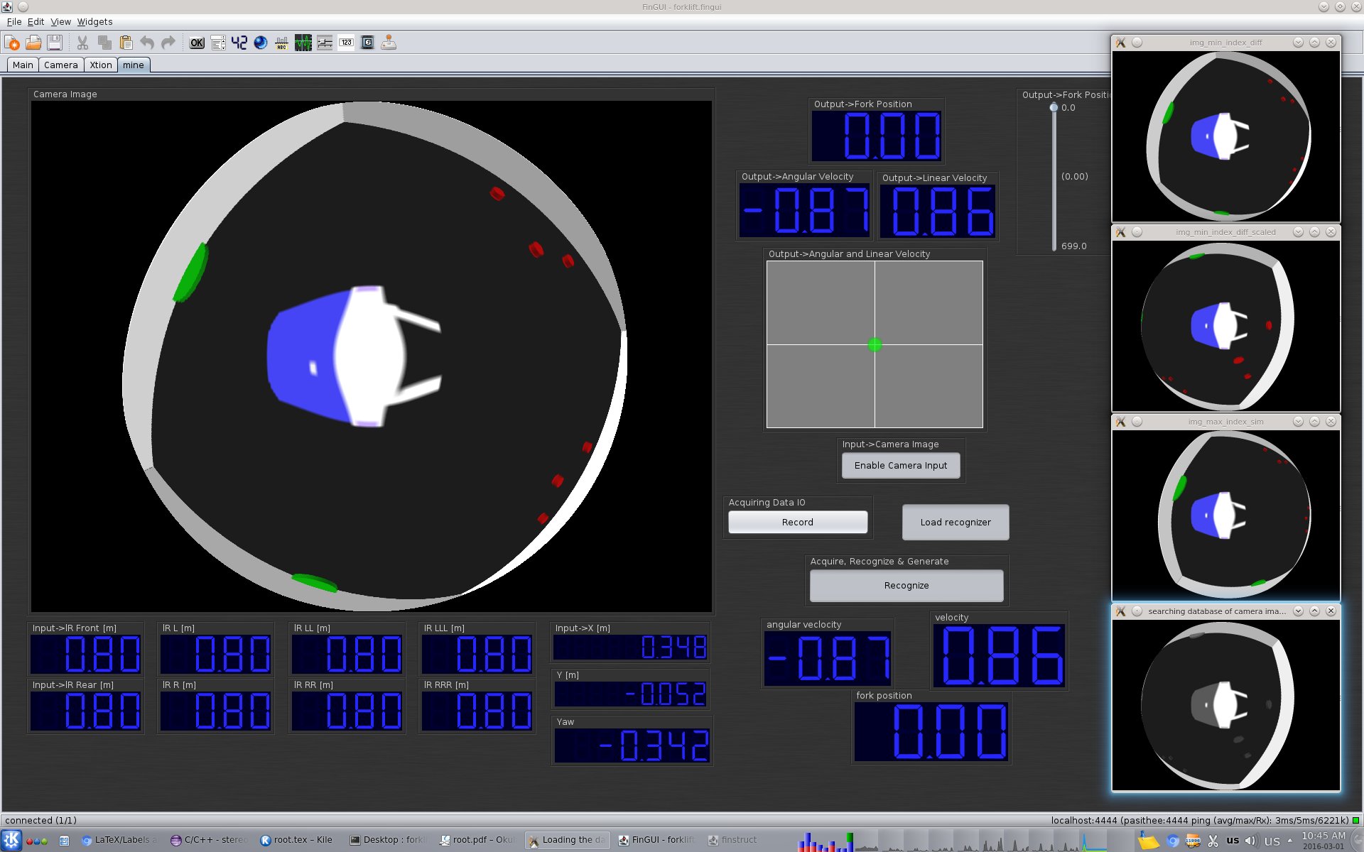
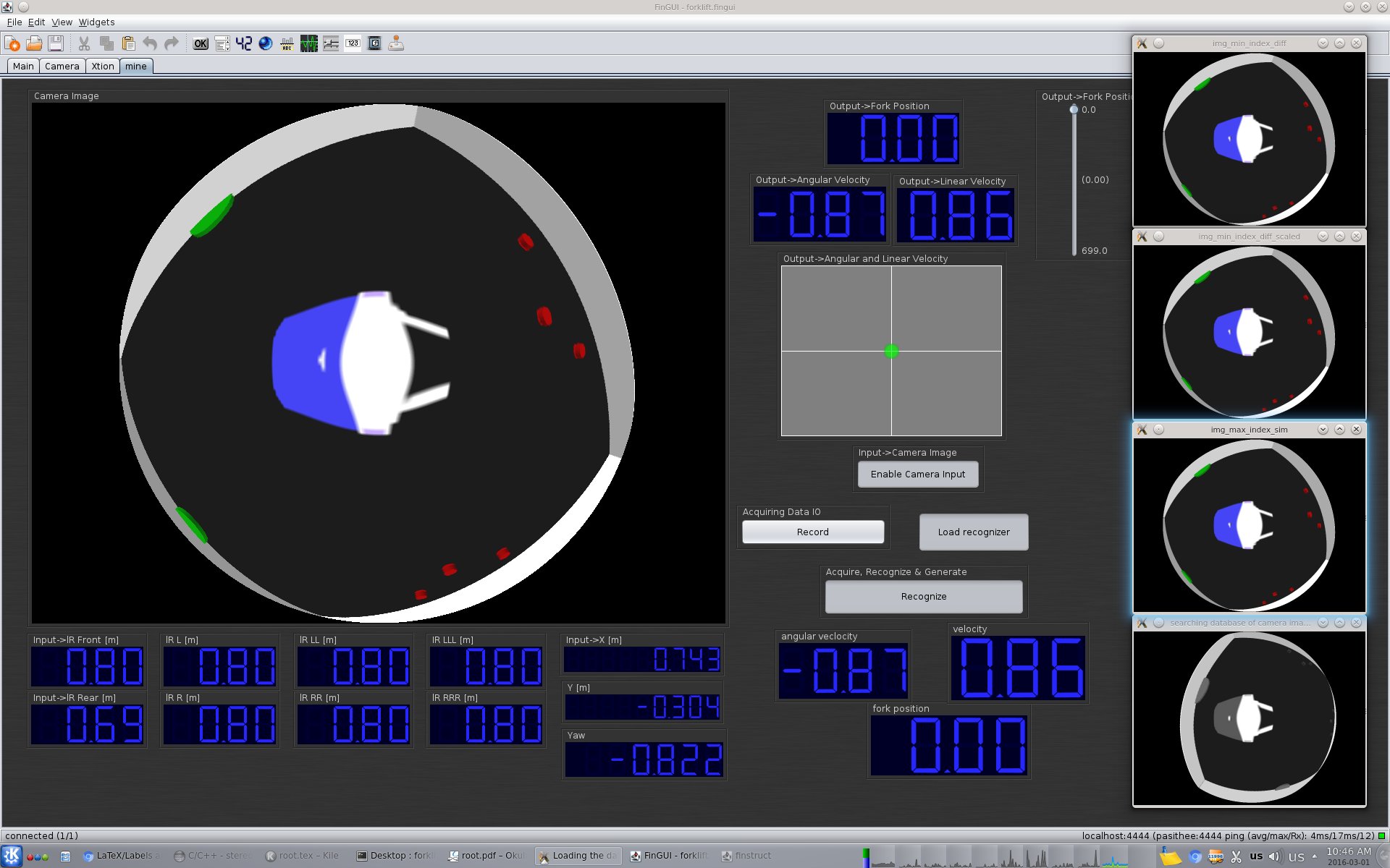
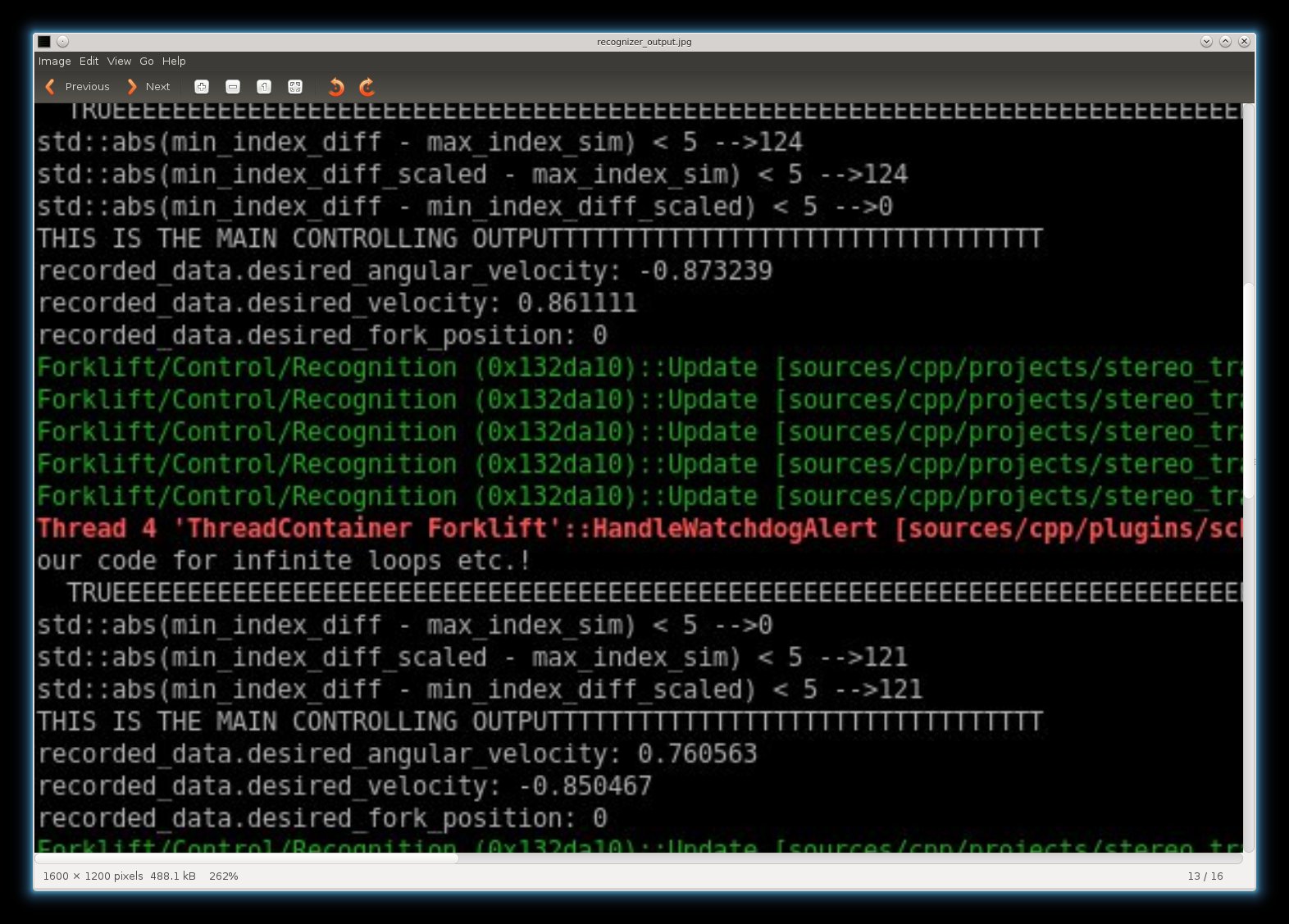
In order to start the intelligent robot control, we start the simulation at first, enable the camera images flow then, and load the recognizer with the learned model and the file path of all the recorded XML files (only the file path). Then the robot does an online recognition as shown in figure 12 and finally the output is generated for controlling the robot which is the corresponding linear velocity and angular velocity of the most similar and least different input $I$ in the memory compared to the new input $I_{t+1}$ as shown in figure 13.

Figure 12: This is how recognizer finds the best match for the input and generates its corresponding output afterwards.

Figure 13: Having found the best match, recognizer generates the corresponding output of the best input in database to the controller input in order to control the robot’s action and next move.

IV Conclusions and Future Work

The goal of this paper was introducing a new conceptual cognitive model which may redefine intelligence and add parameters to intelligence as well as redefining control as a cognition process. The question addressed is how we can generate a specific detailed intelligence with a strong mathematical foundation and also general enough to be applicable to any input data for generating any kinds of output data for control. This is the application of this cognitive model (MLR) in robotics for intelligent control but later on we may also be able to apply this to any other sensor data for any other application as well.

The discussed MLR model is a cognitive process which should be applicable to any kinds of the robot platforms or data structure and data types. For this reason, there are plenty of ideas for applying this model to different applications and different sensor data. More specifically, in the presented experimental results, we still have distance and localization input data as shown in figure  8 which also can be a very interesting quest to apply MLR on them and also their combination as well meaning that applying MLR on all of the sensor data fused together.

There is plenty of room and flexibility in putting this concept into an experiment but we should also notice that learning can be very time-consuming, recognition however should be almost real-time. We need to keep that in mind as well. Also the main power the current model is the ability to handle a high-dimensional data in a way that it reduces the dimensionality without reducing the accuracy of their reconstruction which is a very powerful tool in handling and managing the big-sized data set of different kinds. That is why one of the important future work will be to apply MLR on a huge database of sensor data and use that for intelligent control.

References

- [1] Thrun, Sebastian, et al. ”Stanley: The robot that won the DARPA Grand Challenge.” Journal of field Robotics 23.9 (2006): 661-692.
- [2] Montemerlo, Michael, et al. ”Junior: the stanford entry in the urban challenge.” The DARPA Urban Challenge. Springer Berlin Heidelberg, 2009. 91-123.
- [3] Thrun, Sebastian. ”Toward robotic cars.” Communications of the ACM 53.4 (2010): 99-106.
- [4] Thrun, Sebastian, Wolfram Burgard, and Dieter Fox. Probabilistic robotics. MIT press, 2005.
- [5] LeCun, Yann, Yoshua Bengio, and Geoffrey Hinton. ”Deep learning.” Nature 521.7553 (2015): 436-444.
- [6] Jones, Nicola. ”The learning machines.” (2014): 146-148.
- [7] Schmidhuber, Jürgen. ”Deep learning in neural networks: An overview.” Neural Networks 61 (2015): 85-117.
- [8] Mnih, Volodymyr, et al. ”Human-level control through deep reinforcement learning.” Nature 518.7540 (2015): 529-533.
- [9] Schölkopf, Bernhard. ”Artificial intelligence: Learning to see and act.” Nature 518.7540 (2015): 486-487.
- [10] Littman, Michael L. ”Reinforcement learning improves behaviour from evaluative feedback.” Nature 521.7553 (2015): 445-451.
- [11] www.opencv.org
- [12] www.finroc.org