*[arabic]figure *[arabic]table disposition [toc]toc.1toc.1ContentsContentstoc.1

BONN-TH-2019-02

Abstract

Extensions of the Standard Model often come with additional, possibly electroweakly charged Higgs states, the prototypal example being the Two-Higgs-Doublet Model. While collider phenomenology does not exclude the possibility for some of these new scalar fields to be light, it is relatively natural to consider masses in the multi-TeV range, in which case the only remaining light Higgs boson automatically receives SM-like properties. The appearance of a hierarchy between the new-physics states and the electroweak scale then leads to sizable electroweak corrections, e. g. in the decays of the heavy Higgs bosons, which are dominated by effects of infrared type, namely Sudakov logarithms. Such radiative contributions obviously affect the two-body decays, but should also be paired with the radiation of electroweak gauge bosons (or lighter Higgs bosons) for a consistent picture at the one-loop order. Resummation of the leading terms is also relatively easy to achieve. We re-visit these questions in the specific case of the fermionic decays of heavy Higgs particles in the Next-to-Minimal Supersymmetric Standard Model, in particular pointing out the consequences of the three-body final states for the branching ratios of the heavy scalars.

[]Introduction

Many extensions of the Standard Model (SM) imply the existence of an extended Higgs sector. While the reality of a SM-like Higgs boson is firmly established by the experiments at the Large Hadron Collider (LHC) Aad:2012tfa ; Chatrchyan:2012ufa ; Aad:2015zhl , the status of other Higgs states remains largely speculative. At the moment, the absence of conclusive signals for such new states has only limited implications since, in many models, only a marginal portion of the parameter space has been actually tested. In fact, light electroweakly-charged scalar particles with a mass below that of the top quark continue to be phenomenologically viable Bahl:2018zmf , even though such scenarios receive constraints from multiple directions. The situation is much looser for singlet-dominated states, such as predicted in the Next-to-Minimal Supersymmetric Standard model (NMSSM) for instance (see e. g. Ref. Domingo:2015eea for a discussion of the constraints from Run I at the LHC). On the other hand, it is tempting to retreat to the (multi-)TeV scale for the mass of the new Higgs bosons, because then the SM-like characteristics of the observed state (see Refs. Khachatryan:2016vau ; Sirunyan:2018koj ; Aad:2019mbh ) are almost automatically fulfilled, due to the decoupling properties of the heavy Higgs particles (under the assumption of perturbative couplings). In such a case, however, the presence of a comparatively high scale introduces a hierarchy with respect to the electroweak interactions that could lead to large radiative corrections, typically in the form of Sudakov logarithms—see e. g. Refs. Sudakov:1954sw ; Kuhn:1999nn ; Denner:2000jv for a few related references.

Below, we specialize in the decays of heavy Higgs bosons in the particular case of the NMSSM, although our analysis can be easily extended to any other model including additional Higgs states, in particular models based on a Two-Higgs-Doublet Model (THDM) of type II. The NMSSM Ellwanger:2009dp ; Maniatis:2009re —as any supersymmetric (SUSY) Nilles:1983ge ; Haber:1984rc extension of the SM—shields the mass of the SM-like Higgs against large radiative corrections from new physics at high-energy scales (e. g. the GUT or Planck scale), suggesting a technically natural answer to the ‘Hierarchy Problem’. Other motivations are the resolution of the ‘$\mu$ problem’ Kim:1983dt or the rich phenomenology of the Higgs or neutralino sectors, see e. g. Ellwanger:2015uaz ; Domingo:2015eea ; Conte:2016zjp ; Guchait:2016pes ; Badziak:2016tzl ; Das:2016eob ; Cao:2016uwt ; Das:2017tob ; Muhlleitner:2017dkd ; Ellwanger:2014hia ; Chakraborty:2015xia ; Kim:2015dpa ; Carena:2018nlf ; Titterton:2018pba ; Cao:2016nix ; Xiang:2016ndq ; Cao:2018rix ; Ellwanger:2018zxt ; Domingo:2018ykx for a few recent discussions. The NMSSM contains one pair of charged and four additional neutral Higgs bosons beyond the SM-like state, involving two new ${\cal CP}$-even and two ${\cal CP}$-odd degrees of freedom. Several public tools propose an evaluation of the two-body Higgs decays. The standard has long been a QCD-improved calculation: the decay routines of NMSSMTools Ellwanger:2004xm ; Ellwanger:2005dv ; Domingo:2015qaa ; NMSSMTOOLS-www and NMSSMCALC Baglio:2013iia ; NMSSMCALC-www are based on HDECAY Djouadi:1997yw ; Djouadi:2018xqq ; SOFTSUSY Allanach:2001kg ; Allanach:2013kza ; Allanach:2017hcf also performs at the same order. More recently, full one-loop analyses of the two-body Higgs decays have been performed with the code SloopS sloops-www ; Belanger:2014roa ; Belanger:2016tqb ; Belanger:2017rgu or in the $\overline{\mathrm{DR}}$ $\left(\overline{\mathrm{MS}}\right)$ scheme for generic models Goodsell:2017pdq with the code SPHENO Porod:2003um ; Porod:2011nf ; Goodsell:2014bna ; spheno-www , which employs SARAH Staub:2009bi ; Staub:2010jh ; Staub:2012pb ; Staub:2013tta . Also in Ref. Domingo:2018uim the two-body Higgs decays into SM final states were considered at the full one-loop order. Similar projects have been presented for the THDM and its extensions Krause:2018wmo ; Krause:2019oar ; Kanemura:2019kjg . Yet—with the exception of photon and gluon radiation as well as the production of off-shell gauge bosons below threshold that subsequently decay into fermions (see e. g. Ref. Spira:2016ztx for a recent summary in the MSSM)—little attention has been paid to the three-body decays, which, however, intervene at the same order as the one-loop corrections to two-body decays.

The degeneracy among the states forming an $SU(2)_{\text{L}}$ multiplet is lifted by the electroweak symmetry breaking, so that the mass-squared differences among the partners of a scalar doublet are expected to be of the order of $M_{Z}^{2}$. Therefore, in scenarios of a THDM where one doublet mass is much larger than the electroweak scale, actually four Higgs bosons have almost degenerate large masses and approximately organize as an $SU(2)_{\text{L}}$ doublet, while one Higgs boson is automatically endowed with SM-like properties, thus making it a good candidate for explaining the signals observed by the ATLAS and CMS collaborations—provided its mass falls within the suitable interval at $\mathord{\sim}\,125$ GeV. This setup fulfills the conditions of the decoupling limit Gunion:2002zf and the decays of the heavy Higgs bosons into SM final states tend to be dominated by the fermionic channels: the couplings of the heavy states to a pair of electroweak gauge bosons vanish (approximately for the ${\cal CP}$-even Higgs), because the doublet formed by the heavy states is orthogonal to that generating the electroweak-symmetry-breaking vacuum expectation value (v.e.v.); in addition, the decays into a SM-like Higgs plus an electroweak gauge boson are also suppressed, because the decoupling states are approximately partners of one another under the electroweak gauge group, and not of the SM-like Higgs; finally, Higgs-to-Higgs decays are suppressed in the limit of heavy initial states—the triple Higgs coupling of electroweak size implies a suppression $\mathord{\sim}\,M_{Z}/M_{h}$, where $M_{h}$ represents the mass of the initial Higgs boson. On the other hand, at least some of the fermionic decays are expected to be unsuppressed, depending on the type of THDM. For a type II framework, the standard search channels at the LHC thus involve tau-onic final states, while the $b\bar{b}$ or $t\bar{t}$ decays are actually sizable but suffer from the QCD background. The decays of singlet-dominated states are more difficult to characterize generically. A pure singlet could only decay radiatively into SM final states (and even not at all for $\lambda=0$). In general, the decays of mostly singlet-like states into SM particles are thus dominated by their subleading doublet components—therefore their bosonic decays, e. g. into light Higgs bosons, are not necessarily suppressed. Below, we focus on the fermionic decays for simplicity, but the procedure can be generalized to bosonic final states as well.

It was observed in Ref. Domingo:2018uim that the decays of heavy new-physics Higgs states into SM particles could receive sizable radiative corrections beyond the well-known QCD effects Braaten:1980yq ; Drees:1990dq . It is desirable to control such corrections for a better characterization of the expected signals at colliders and a more quantitative implementation of associated limits. At the LHC, the expected reach does not exceed masses of $\mathord{\sim}\,2$ TeV CMS:2016DP . However, already for masses in the TeV range, so-called electroweak Sudakov double logarithms

$$\mathord{\sim}\,\frac{g_{2}^{2}}{16\pi^{2}}\ln^{2}\frac{M_{V}^{2}}{M_{h}^{2}}$$ (1)

(where $g_{2}$ represents the gauge coupling, and $M_{V}$ and $M_{h}\sim 1$–$2$ TeV denote the masses of the gauge and heavy Higgs bosons respectively) attain the level of $\mathord{\sim}\,10\%$.

The main purpose of this paper consists in analyzing the electroweak corrections to the two-body fermionic decays of heavy Higgs bosons, and their interplay with three-body decays involving the radiation of an electroweak gauge boson. The noteworthy difference compared to the case of QED and QCD corrections is that the radiation of massive electroweak gauge bosons leads to clearly distinguishable final states, as opposed to soft and collinear photons and gluons. The corresponding decays could thus be measured separately and there is no justification on the theoretical side for considering only inclusive decay widths (summing over two-body decays and the corresponding ones with radiated $W,Z$): therefore the potentially large Sudakov double logarithms are experimentally accessible effects that are expected to reduce the branching fractions of the two-body decays. In any case, from order-counting it appears mandatory to take the three-body final states into account if one wants to perform a consistent analysis of the branching ratios for two-body decays of heavy Higgs bosons at the full one-loop order. To our knowledge, such effects have not been considered in the NMSSM (or the MSSM) yet, and we expose here how we implement these channels in view of a future inclusion within a version of FeynHiggs Heinemeyer:1998np ; Heinemeyer:1998yj ; Degrassi:2002fi ; Frank:2006yh ; Hahn:2013ria ; Bahl:2016brp ; Bahl:2017aev ; FH-www dedicated to the NMSSM Drechsel:2016jdg ; Domingo:2017rhb ; Domingo:2018uim .

In the following section, we discuss the formal aspects of our evaluation of the two- and three-body decays, emphasizing the possibility to capture most of the electroweak corrections within a simple resummation of Sudakov double logarithms Fadin:1999bq . We then illustrate the numerical impact of the electroweak corrections in a scenario with heavy SUSY sector and focusing on doublet-dominated Higgs bosons in the initial state. Finally, Sect. 7 summarizes our achievements. []Higgs decays into SM fermions in the NMSSM

In this section, we summarize the main theoretical ingredients entering the decays of heavy Higgs bosons into SM fermions. We follow the notations of Refs. Domingo:2017rhb ; Domingo:2018uim .

Two-body decay width

Decay of the Higgs bosons at one-loop order: automated calculation

We already described our full one-loop implementation of the two-body fermionic decays of neutral Higgs bosons in Ref. Domingo:2018uim . For the sake of completeness, we summarize the main ingredients in the following:

• We rely on the automated calculation of FeynArts Kublbeck:1990xc ; Hahn:2000kx , FormCalc Hahn:1998yk and LoopTools Hahn:1998yk , using the model file (and renormalization scheme) presented in Ref. Domingo:2017rhb .

• External Higgs fields are upgraded to on-shell fields using the transformation matrix $Z^{\mbox{\tiny mix}}$ that is determined by the LSZ reduction, see Ref. Domingo:2017rhb . The mixing of the external Higgs leg with the electroweak neutral current is processed diagrammatically, and we subtract gauge-violating effects of two-loop order that appear due to the difference between the (kinematical) loop-corrected Higgs mass and the tree-level mass, see Ref. Domingo:2018uim . The fermion fields are renormalized on-shell.

• The virtual QCD and QED corrections are processed separately and combined with the real-radiation contributions in order to define an infrared (IR)-finite correction factor Braaten:1980yq ; Drees:1990dq ; Dabelstein:1995js to the pure born width $\Gamma^{\text{Born}}$ describing the inclusive fermionic width (with radiated gluons and photons in the final state). The QCD logarithms are absorbed within the definition of running Yukawa couplings evaluated at the scale of the decaying Higgs:

  $$\frac{\Gamma^{\text{QCD+QED}}}{\Gamma^{\text{Born}}} =\left(\frac{Y_{f}{(M_{h})}}{Y_{f}{(m_{t})}}\right)^{2}\left[1+c^{\text{QCD}}+c^{\text{QED}}\right]$$ (2)

  where $Y_{f}$ represents the relevant Yukawa coupling absorbing QCD logarithms; $c^{\text{QCD}}$ and $c^{\text{QED}}$ represent the QCD and QED correction factors—see e. g. Eq. (2.12) of Ref. Domingo:2018uim .

• The leading SUSY corrections amount to contributions to effective dimension $4$ Higgs–fermion operators. They are explicitly extracted in the $SU(2)$-conserving limit and re-arranged so as to provide a resummation of the $\tan\beta$-enhanced effects, see Refs. Banks:1987iu ; Hall:1993gn ; Hempfling:1993kv ; Carena:1994bv ; Carena:1999py ; Eberl:1999he ; Degrassi:2000qf ; Buras:2002vd ; Guasch:2003cv ; Noth:2008tw ; Noth:2010jy ; Williams:2011bu ; Baglio:2013iia ; Ghezzi:2017enb ; a linearized (non-resummed) version is subtracted from the actual one-loop diagrammatic calculation in order to avoid double counting.

• The full one-loop corrections (excluding the QED and QCD corrections) to the Higgs–fermion vertex are derived automatically from our model file. However, we subtract gauge-violating effects of two-loop order through a re-definition of the Higgs–Goldstone couplings by a shift of one-loop order, as explained in section 2.1 of Ref. Domingo:2018uim .

Obviously, the two-body decays of the charged Higgs can be implemented in a similar fashion. In particular:

• The external charged Higgs field and its mass are renormalized on-shell, thus requiring no normalization factor. The mixing with the electroweak charged current is processed diagrammatically.

• The QCD and QED corrections are factorized out and combined with the real radiation process. The QCD-correction factor is well-known Djouadi:1994gf . The QED contribution is somewhat more involved, due to the initial state being electrically charged. We compute this correction factor by considering separately the virtual piece as well as the soft and hard radiation. For the hard radiation, we explicitly take the limit $m_{b}\to 0$. For simplicity, we only provide the leading logarithmic terms for $H^{-}\to b\bar{t}$ below:

  $$\frac{\Delta\Gamma^{\text{QED}}}{\Gamma^{\text{Born}}}[\mbox{$H^{-}\to b\bar{t}\,$}] =\frac{e^{2}}{16\,\pi^{2}}\left[C^{\text{virt}}+C^{\text{soft}}+C^{\text{hard}}\right],$$ (3a)

  $$C^{\text{virt}} =2\left[Q_{b}^{2}\,\ln\frac{m_{b}^{2}}{M_{H^{\pm}}^{2}}+Q_{t}^{2}\,\ln\frac{m_{t}^{2}}{M_{H^{\pm}}^{2}}+2\left(1+Q_{b}\,Q_{t}\right)\right]\ln\frac{M_{H^{\pm}}^{2}}{m_{\gamma}^{2}}\,,$$ (3b)

  $$\begin{split}C^{\text{soft}}&=2\left[Q_{b}^{2}\,\ln\frac{m_{b}^{2}}{M_{H^{\pm}}^{2}}+Q_{t}^{2}\,\ln\frac{m_{t}^{2}}{M_{H^{\pm}}^{2}}+2\left(1+Q_{b}\,Q_{t}\right)\right]\ln\frac{m_{\gamma}^{2}}{\Omega^{2}_{\text{IR}}}\\ &\quad-Q_{b}^{2}\left[\ln^{2}\frac{m_{b}^{2}}{M_{H^{\pm}}^{2}}+2\,\ln\frac{m_{b}^{2}}{M_{H^{\pm}}^{2}}\right]-Q_{t}^{2}\left[\ln^{2}\frac{m_{t}^{2}}{M_{H^{\pm}}^{2}}+2\,\ln\frac{m_{t}^{2}}{M_{H^{\pm}}^{2}}\right],\end{split}$$ (3c)

  $$\begin{split}C^{\text{hard}}&=2\left[Q_{b}^{2}\,\ln\frac{m_{b}^{2}}{M_{H^{\pm}}^{2}}+Q_{t}^{2}\,\ln\frac{m_{t}^{2}}{M_{H^{\pm}}^{2}}+2\left(1+Q_{b}\,Q_{t}\right)\right]\ln\frac{\Omega^{2}_{\text{IR}}}{M_{H^{\pm}}^{2}}\\ &\quad+3\left[Q_{b}^{2}\,\ln\frac{m_{b}^{2}}{M_{H^{\pm}}^{2}}+Q_{t}^{2}\,\ln\frac{m_{t}^{2}}{M_{H^{\pm}}^{2}}\right],\end{split}$$ (3d)

  where $e$ represents the electric charge, $Q_{t,b}$ the fermion charges, $m_{\gamma}$ the photon-mass regulator, and $\Omega_{\text{IR}}$ the IR cut on the photon energy.

• Non-QCD and non-QED one-loop diagrams are calculated with our automated procedure.

Below, we denote the decay widths that are derived in this automated fashion at fixed order as $\Gamma^{\text{FO}}$, while the Born results read $\Gamma^{\text{Born}}$. As in Ref. Domingo:2018uim , the renormalization scale is set equal to the pole top mass $m_{t}=173.2$ GeV for all $\overline{\mathrm{DR}}$-renormalized counterterms. As we wish to focus on the electroweak corrections, we will in practice consider a scenario with decoupling (heavy) SUSY particles. In this context, the SUSY corrections essentially reduce to their contributions to the dimension $4$ effective operators—see Refs. Banks:1987iu ; Hall:1993gn ; Hempfling:1993kv ; Carena:1994bv ; Carena:1999py ; Eberl:1999he ; Degrassi:2000qf ; Buras:2002vd ; Guasch:2003cv ; Noth:2008tw ; Noth:2010jy ; Williams:2011bu ; Baglio:2013iia ; Ghezzi:2017enb —and we thus fully factorize them as corresponding to a short-distance effect. In this procedure, however, also the SUSY contributions to the Higgs wave function—i. e. intervening in the normalization of the $Z^{\text{mix}}$ matrix—need to be extracted accordingly. This effective tree-level width, including SUSY corrections, is later denoted as $\Gamma^{\text{eff}}$. Then, in Ref. Domingo:2018uim , we kept the term of the squared one-loop amplitude in the definition of the width: this was justified in the case where one-loop contributions dominate over the tree-level result. However, the electroweak corrections that we study below are essentially proportional to the tree-level amplitude, meaning that they would be suppressed together with it. In this case, the full one-loop squared term is actually misleading, since its impact can be substantially altered by the inclusion of the interference of the amplitude of two-loop order with the tree-level one. We thus discard this term, keeping only a squared one-loop amplitude for those contributions that are not proportional to the tree-level term (and subleading in the channels that we are considering).

Electroweak double logarithms

In this one-loop evaluation of the two-body fermionic decays of heavy Higgs bosons, several pieces of the radiative corrections beyond the QCD and QED contributions can matter, in general. However, in the limit of heavy SUSY spectra, most of the SUSY-related corrections are logarithmic and can be captured within effective Yukawa couplings, as mentioned above. As can be observed e. g. in Fig. 1 of Ref. Domingo:2018uim (by comparing the green and red curves), this effective description, which works reasonably well for a light Higgs, still leaves out sizable one-loop effects for a heavy state. These remaining one-loop contributions (reaching $\mathord{\sim}\,10\%$ for the $1$ TeV states of Fig. 1 of Ref. Domingo:2018uim ) are associated with electroweak corrections. Below, we explain how most of these relatively large effects can be easily put under control.

Figure 1: Contributions to $h_{i}\to b\bar{b}$ leading to double logarithms.

The sizable electroweak contribution originates in the hierarchy between the heavy Higgs state and the light particles entering in the loops, which results in large logarithms of Sudakov type. In particular, for gauge interactions we expect to find double logarithms $\mathord{\sim}\,g_{2}^{2}/\left(16\,\pi^{2}\right)\ln^{2}{\left(M_{Z}^{2}/M_{h}^{2}\right)}$. The diagrams leading to double logarithms in the example of $h_{i}\to b\bar{b}$ are displayed in Fig. 1 and include two topologies:

1. the well-known fermion–fermion–vector triangle:
   the associated loop-function contributes $\mathord{\sim}\,\frac{1}{2}\ln^{2}{\left(M_{V}^{2}/M_{h}^{2}\right)}$ at the double-logarithmic order;

2. the fermion–scalar–vector triangle:
   under the condition that the internal scalar is almost degenerate with the external Higgs, the loop function contributes $\mathord{\sim}\,{-}\frac{1}{4}\ln^{2}{\left(M_{V}^{2}/M_{h}^{2}\right)}$; here, ‘almost degenerate’ covers a range larger than $M_{h}\pm M_{V}$, but much narrower than $\left[M_{h}/2,\,2\,M_{h}\right]$.

In our case, one cannot rely on the popular evaluations of the double-logarithmic coefficient presented in Refs. Denner:2000jv ; Fadin:1999bq , amounting to a sum of the quantity

$$-\frac{g_{2}^{2}}{32\,\pi^{2}}\left[I\left(I+1\right)+\left(Y/2\right)^{2}\,t_{\text{w}}^{2}-Q^{2}\,s_{\text{w}}^{2}\right]\ln^{2}{\frac{M_{V}^{2}}{M_{h}^{2}}}$$ (4)

over the external legs—where $I$, $Y$, $Q$ represent the isospin, hypercharge and electric charge of the external state, $t_{\text{w}}$ and $s_{\text{w}}$ denote the tangent and sine of the electroweak mixing angle; the $Q^{2}$ term subtracts the QED contribution that is considered separately. The reason why this formula fails is simply that one of the (electroweakly charged) external states, the Higgs line, is massive, actually determining the center-of-mass energy.

For a doublet state $h_{i}$ or $H^{\pm}$ in the decoupling limit, the electroweak partners of the external Higgs bosons are indeed always almost degenerate with the external state and it is easy to extract the Sudakov double logarithms explicitly (with $g_{1,2}$ the electroweak couplings; for $H^{-}\to t\bar{b}$, the subscripts $t,b$ refer to the pieces of the width that are proportional to the squared Yukawa couplings $Y_{t,\,b}^{2}$):

$$\frac{\Delta\Gamma^{\text{DL}}}{\Gamma^{\text{Born}}}{\left[\mbox{\mbox{$h_{i}\to b\bar{b}\,$}}\right]} \simeq-\frac{1}{48\,\pi^{2}}\left[\frac{5}{12}\,g_{1}^{2}+\frac{9}{4}\,g_{2}^{2}-\frac{2}{3}\,e^{2}\right]\ln^{2}\frac{M_{V}^{2}}{M_{h_{i}}^{2}}\,,$$ (5a)

$$\frac{\Delta\Gamma^{\text{DL}}}{\Gamma^{\text{Born}}}{\left[\mbox{\mbox{$h_{i}\to t\bar{t}\,$}}\right]} \simeq-\frac{1}{48\,\pi^{2}}\left[\frac{17}{12}\,g_{1}^{2}+\frac{9}{4}\,g_{2}^{2}-\frac{8}{3}\,e^{2}\right]\ln^{2}\frac{M_{V}^{2}}{M_{h_{i}}^{2}}\,,$$ (5b)

$$\frac{\Delta\Gamma^{\text{DL}}}{\Gamma^{\text{Born}}}{\left[\mbox{\mbox{$h_{i}\to\tau^{+}\tau^{-}$}}\right]} \simeq-\frac{1}{48\,\pi^{2}}\left[\frac{15}{4}\,g_{1}^{2}+\frac{9}{4}\,g_{2}^{2}-6\,e^{2}\right]\ln^{2}\frac{M_{V}^{2}}{M_{h_{i}}^{2}}\,,$$ (5c)

$$\frac{\Delta\Gamma^{\text{DL}}_{b}}{\Gamma^{\text{Born}}_{b}}{\left[\mbox{\mbox{$H^{-}\to t\bar{b}\,$}}\right]} \simeq-\frac{1}{48\,\pi^{2}}\left[\frac{5}{12}\,g_{1}^{2}+\frac{9}{4}\,g_{2}^{2}-\frac{5}{3}\,e^{2}\right]\ln^{2}\frac{M_{V}^{2}}{M_{H^{\pm}}^{2}}\,,$$ (5d)

$$\frac{\Delta\Gamma^{\text{DL}}_{t}}{\Gamma^{\text{Born}}_{t}}{\left[\mbox{\mbox{$H^{-}\to t\bar{b}\,$}}\right]} \simeq-\frac{1}{48\,\pi^{2}}\left[\frac{17}{12}\,g_{1}^{2}+\frac{9}{4}\,g_{2}^{2}-\frac{5}{3}\,e^{2}\right]\ln^{2}\frac{M_{V}^{2}}{M_{H^{\pm}}^{2}}\,,$$ (5e)

$$\frac{\Delta\Gamma^{\text{DL}}}{\Gamma^{\text{Born}}}{\left[\mbox{\mbox{$H^{-}\to\tau^{-}\bar{\nu}_{\tau}$}}\right]} \simeq-\frac{1}{48\,\pi^{2}}\left[\frac{15}{4}\,g_{1}^{2}+\frac{9}{4}\,g_{2}^{2}-3\,e^{2}\right]\ln^{2}\frac{M_{V}^{2}}{M_{H^{\pm}}^{2}}\,.$$ (5f)

Here again, the terms $\mathord{\propto}\,e^{2}$ simply correspond to the QED corrections, which are subtracted since they are separately processed as a long-distance effect. We stress that the double-logarithmic corrections always interfere destructively with the tree-level amplitude, thus leading to a systematic reduction of the two-body decay width.

For a singlet-dominated state, the situation is somewhat more subtle. If the mass of this Higgs boson is far from that of other Higgs states, then the fermion–scalar–vector triangle does not produce double-logarithms for lack of a degenerate electroweak partner of the external state. In this case, the double-logarithmic terms coincide with the formula of Eq. (4), applied to the fermionic final states (one being left-handed, the other right-handed). However, if the singlet finds itself accidentally in the window of mass degeneracy with the doublet states, then the fermion–scalar–vector topology is relevant, together with possibly substantial doublet-singlet mixing.

For Higgs masses in the range of a few TeV, we expect electroweak corrections to remain at the level of $\mathord{\sim}\,10\%$: this is still perturbative and there is no deep call for resumming these corrections. This only becomes necessary if one desires to extend the result to masses as high as $\mathcal{O}{\left(100\right)}$ TeV. On the other hand, it is remarkable that the leading double-logarithmic terms can be controlled at all orders. Such a resummation also allows us to define an effective tree-level result capturing the bulk of the radiative effects. The resummation of double logarithms can be performed by considering the IR behavior of the matrix element, see Ref. Fadin:1999bq : it eventually amounts to exponentiating the double-logarithmic coefficient obtained at the one-loop order. We stress that there is no complication from the separate treatment of the QED effects at the considered order. We can define the ‘electroweakly improved’ Born width $\Gamma^{\text{EW}}$ as

$$\frac{\Gamma^{\text{EW}}}{\Gamma^{\text{Born}}} =\exp\left[\frac{\Delta\Gamma^{\text{DL}}}{\Gamma^{\text{Born}}}\right].$$ (6)

In the ${\cal CP}$-violating case, there is no difficulty in processing the scalar and pseudoscalar components separately, since the corresponding operators do not interfere.

Single logarithms

While we expect the double logarithms to represent the numerically largest piece of the electroweak corrections, it is relatively easy to extract single logarithms as well. The latter originate in the vertex corrections of Fig. 1, but also in the counterterm and wave-function normalization $Z^{\mbox{\tiny mix}}$. Obviously, they depend on the chosen scheme, i. e. the definition of the tree-level Yukawa couplings. In our ‘on-shell’ definition and with the renormalization scale of the loop functions set to $m_{t}\sim M_{Z}$ (following the prescriptions of FeynHiggs), we obtain the following terms for the decays of doublet states (neglecting $Y_{\tau}^{2}$):

$$\frac{\Delta\Gamma^{\text{SL}}}{\Gamma^{\text{Born}}}{\left[\mbox{\mbox{$h_{i}\to b\bar{b}\,$}}\right]} \simeq\frac{1}{16\,\pi^{2}}\left[3\,Y_{b}^{2}\left(1+c_{\beta}^{2}\right)-Y_{t}^{2}\left(2+c_{\beta}^{2}\right)\right]\ln\frac{M_{h_{i}}^{2}}{M_{Z}^{2}}\,,$$ (7a)

$$\frac{\Delta\Gamma^{\text{SL}}}{\Gamma^{\text{Born}}}{\left[\mbox{\mbox{$h_{i}\to t\bar{t}\,$}}\right]} \simeq\frac{1}{16\,\pi^{2}}\left[3\,Y_{t}^{2}\left(1+s_{\beta}^{2}\right)-Y_{b}^{2}\left(2+s_{\beta}^{2}\right)\right]\ln\frac{M_{h_{i}}^{2}}{M_{Z}^{2}}\,,$$ (7b)

$$\frac{\Delta\Gamma^{\text{SL}}}{\Gamma^{\text{Born}}}{\left[\mbox{\mbox{$h_{i}\to\tau^{+}\tau^{-}$}}\right]} \simeq\frac{1}{16\,\pi^{2}}\left[3\,Y_{b}^{2}\left(1+c_{\beta}^{2}\right)-3\,Y_{t}^{2}\,c_{\beta}^{2}\right]\ln\frac{M_{h_{i}}^{2}}{M_{Z}^{2}}\,,$$ (7c)

$$\frac{\Delta\Gamma^{\text{SL}}_{b}}{\Gamma^{\text{Born}}_{b}}{\left[\mbox{\mbox{$H^{-}\to t\bar{b}\,$}}\right]} \simeq\frac{1}{16\,\pi^{2}}\left[3\,Y_{b}^{2}\left(1+c_{\beta}^{2}\right)-Y_{t}^{2}\left(2+c_{\beta}^{2}\right)\right]\ln\frac{M_{H^{\pm}}^{2}}{M_{Z}^{2}}\,,$$ (7d)

$$\frac{\Delta\Gamma^{\text{SL}}_{t}}{\Gamma^{\text{Born}}_{t}}{\left[\mbox{\mbox{$H^{-}\to t\bar{b}\,$}}\right]} \simeq\frac{1}{16\,\pi^{2}}\left[3\,Y_{t}^{2}\left(1+s_{\beta}^{2}\right)-Y_{b}^{2}\left(2+s_{\beta}^{2}\right)\right]\ln\frac{M_{H^{\pm}}^{2}}{M_{Z}^{2}}\,,$$ (7e)

$$\frac{\Delta\Gamma^{\text{SL}}}{\Gamma^{\text{Born}}}{\left[\mbox{\mbox{$H^{-}\to\tau^{-}\bar{\nu}_{\tau}$}}\right]} \simeq\frac{1}{16\,\pi^{2}}\left[3\,Y_{b}^{2}\left(1+c_{\beta}^{2}\right)-3\,Y_{t}^{2}\,c_{\beta}^{2}\right]\ln\frac{M_{H^{\pm}}^{2}}{M_{Z}^{2}}\,.$$ (7f)

We note that the terms proportional to gauge couplings cancel out (between the vertex contributions and the Higgs wave-function correction), leaving only terms proportional to the Yukawa couplings. The single logarithms are both of ultra-violet (UV) and IR origins. A resummation would disentangle both types, attributing the UV logarithms to the running of the parameters. In practice, however, we observe that $\ln{\left(M_{h}^{2}/M_{Z}^{2}\right)}\lesssim\pi^{2}$, so that constant pieces (i. e. not depending on $M_{h}$, as opposed to the double- and single-logarithmic terms, in an expansion at $M_{h}\to\infty$) compete with the single logarithms, making a resummation of the latter superfluous.

‘Improved’ width

We schematically summarize the expression of the ‘improved’ prediction of the two-body decay widths with resummed Sudakov double logarithms and factorized SUSY corrections by the following equation:

$$\Gamma^{\text{imp}} =\frac{\Gamma^{\text{QCD+QED}}}{\Gamma^{\text{Born}}}\left\{\Gamma^{\text{FO}}+\Gamma^{\text{eff}}\left(\exp\left[\frac{\Delta\Gamma^{\text{DL}}}{\Gamma^{\text{Born}}}\right]-\left[1+\frac{\Delta\Gamma^{\text{DL}}}{\Gamma^{\text{Born}}}\right]\right)\!\right\}$$ (8)

where $\Gamma^{\text{Born}}$, $\Gamma^{\text{eff}}$, $\Gamma^{\text{QCD+QED}}$ and $\Gamma^{\text{FO}}$ have already been defined above. The shift $\Delta\Gamma^{\text{DL}}$ is obtained directly from the width $\Gamma^{\text{FO}}$ that is derived from the automated calculation at fixed order by substituting the loop functions with the associated double logarithms. In Eq. (8), the two subtracted terms in the square brackets avoid double counting between the ‘tree-level improved’ width $\Gamma^{\text{eff}}\,\exp{\left(\Delta\Gamma^{\text{DL}}/\Gamma^{\text{Born}}\right)}$ and the full fixed-order one-loop width $\Gamma^{\text{FO}}$.

Real radiation

Full calculation

From the perspective of order-counting, the three-body decay widths at the tree level are of the same order as one-loop corrections to the two-body decays. For a full one-loop evaluation of the total widths (and branching ratios) of the Higgs bosons, it is thus mandatory to include these channels in the analysis. If we restrict ourselves to non-SUSY final states, the only possible relevant three-body final states involve the radiation of gauge bosons or light Higgs bosons. The radiation of photons and gluons was actually already taken into account above, hence included within the two-body decay widths.

Using FeynArts and FormCalc, we perform the calculation of the widths at the tree-level order for the following channels: $h_{i}\to Zf\bar{f}$, $H^{\pm}\to W^{\pm}f\bar{f}$, $h_{i}\to h_{j}f\bar{f}$ for $f\in\{b,t,\tau\}$, and $h_{i}\to W^{-}f\bar{f^{\prime}}$, $h_{i}\to W^{+}f^{\prime}\bar{f}$, $h_{i}\to H^{-}f\bar{f^{\prime}}$, $h_{i}\to H^{+}f^{\prime}\bar{f}$, $H^{+}\to Zf\bar{f^{\prime}}$, $H^{+}\to h_{j}f\bar{f^{\prime}}$ for $(f,f^{\prime})\in\{(t,b),(\tau^{+},\nu_{\tau})\}$. We stress that contrarily to the radiation of photons and gluons, these final states are clearly distinguishable from the fermionic two-body channels, so that there is no deep reason to consider (only) inclusive decay widths from a theoretical perspective.

The kinematical integral can be performed (e. g.) in the rest frame of the fermion pair in the final state. There, only two steps of integration are non-trivial, one applying to an ‘angular’ variable, the other to the invariant mass-squared $s$ of the fermion pair. We perform the angular integral analytically, while that on $s$ is carried out numerically. The internal lines are systematically regularized by inserting the total width $\Gamma$ of the corresponding particles in the propagators. These ‘internal’ widths are calculated from the sum of all relevant two-body processes at the tree level.

Having set up the calculation in this way, the leading terms in the squared amplitudes scale like $\Gamma{\left[\mbox{$h\to Vf\bar{f}^{\prime}$}\right]}/\Gamma{\left[\mbox{$h\to f\bar{f}^{\prime}$}\right]}\propto M_{h}^{2}/M_{V}^{2}$. This would lead to the unphysical situation where the three-body decay widths grow faster than the two-body widths, and eventually dominate the decays. However, these contributions linear in $M_{h}^{2}/M_{V}^{2}$ sum up to zero as long as the heavy Higgs doublets decouple from the electroweak sector. For the sake of not spoiling the physical interpretation, it is thus paramount to preserve these decoupling properties of the heavy Higgs states at the level of the loop-corrected Higgs-mixing matrix.

On-shell contributions

When an internal line can be exchanged on-shell, the corresponding contribution near the pole (after dismissing the quadratically growing terms discussed above) is dominated by the narrow-width approximation. In this case, a piece of the three-body width is already accounted for at the level of the two-body widths. Therefore, we subtract such on-shell contributions explicitly. This step is performed by evaluating the two-body widths and branching ratios that intervene in the considered process at the tree level. It is crucial that the full widths that are employed as regulators in the internal lines are computed at exactly the same order as these intermediate two-body widths.

We note that the narrow-width approximation tends to overestimate the contribution from the on-shell pole $M$: this can be easily understood by comparing the lorentzian distribution and its limit for $\Gamma\to 0$,

$$\left[(s-M^{2})^{2}+M^{2}\,\Gamma^{2}\right]^{-1} \xrightarrow{\Gamma\to 0}\frac{\pi}{M\,\Gamma}\,\delta{\left(s-M^{2}\right)}\,.$$ (9)

Consequently, the subtraction of the on-shell contributions can result in an apparent negative width (as long as the Sudakov terms remain subleading), which, however, should be interpreted as a correction applying to the two-body width.

In addition, we expect the radiation of electroweak gauge bosons and Higgs bosons to produce Sudakov double and single logarithms again, when compared to the corresponding two-body width at the Born level. It is useful to extract them explicitly.

Double logarithms

The double logarithms are associated with the radiation of electroweak gauge bosons. The topologies leading to Sudakov logarithms are summarized in Fig. 2 for the example of $h_{i}\to W^{-}t\bar{b}$. The topology with an internal Higgs line is relevant only if the external and internal states are close in mass. For heavy doublet-like Higgs bosons in the initial state, we obtain:

$$\frac{\Gamma^{\text{DL}}{\left[\mbox{\mbox{$h_{i}\to Zb\bar{b}\,$}}\right]}}{\Gamma^{\text{Born}}{\left[\mbox{\mbox{$h_{i}\to b\bar{b}\,$}}\right]}} \simeq\frac{1}{48\,\pi^{2}}\left[\frac{5}{12}\,g_{1}^{2}+\frac{3}{4}\,g_{2}^{2}-\frac{2}{3}\,e^{2}\right]\ln^{2}\frac{M_{V}^{2}}{M_{h_{i}}^{2}}\,,$$ (10a)

$$\frac{\Gamma^{\text{DL}}{\left[\mbox{\mbox{$h_{i}\to Zt\bar{t}\,$}}\right]}}{\Gamma^{\text{Born}}{\left[\mbox{\mbox{$h_{i}\to t\bar{t}\,$}}\right]}} \simeq\frac{1}{48\,\pi^{2}}\left[\frac{17}{12}\,g_{1}^{2}+\frac{3}{4}\,g_{2}^{2}-\frac{8}{3}\,e^{2}\right]\ln^{2}\frac{M_{V}^{2}}{M_{h_{i}}^{2}}\,,$$ (10b)

$$\frac{\Gamma^{\text{DL}}{\left[\mbox{\mbox{$h_{i}\to Z\tau^{+}\tau^{-}$}}\right]}}{\Gamma^{\text{Born}}{\left[\mbox{\mbox{$h_{i}\to\tau^{+}\tau^{-}$}}\right]}} \simeq\frac{1}{48\,\pi^{2}}\left[\frac{15}{4}\,g_{1}^{2}+\frac{3}{4}\,g_{2}^{2}-6\,e^{2}\right]\ln^{2}\frac{M_{V}^{2}}{M_{h_{i}}^{2}}\,,$$ (10c)

$$\frac{\Gamma^{\text{DL}}_{b}{\left[\mbox{\mbox{$h_{i}\to W^{-}t\bar{b}\,$}}\right]}}{\Gamma^{\text{Born}}{\left[\mbox{\mbox{$h_{i}\to b\bar{b}\,$}}\right]}} \simeq\frac{\Gamma^{\text{DL}}_{t}{\left[\mbox{\mbox{$h_{i}\to W^{-}t\bar{b}\,$}}\right]}}{\Gamma^{\text{Born}}{\left[\mbox{\mbox{$h_{i}\to t\bar{t}\,$}}\right]}}\simeq\frac{\Gamma^{\text{DL}}{\left[\mbox{\mbox{$h_{i}\to W^{-}\tau^{+}\nu_{\tau}$}}\right]}}{\Gamma^{\text{Born}}{\left[\mbox{\mbox{$h_{i}\to\tau^{+}\tau^{-}$}}\right]}}\simeq\frac{g_{2}^{2}}{64\,\pi^{2}}\ln^{2}\frac{M_{V}^{2}}{M_{h_{i}}^{2}}\,,$$ (10d)

$$\frac{\Gamma^{\text{DL}}_{b}{\left[\mbox{\mbox{$H^{-}\to Zb\bar{t}\,$}}\right]}}{\Gamma^{\text{Born}}_{b}{\left[\mbox{\mbox{$H^{-}\to b\bar{t}\,$}}\right]}} \simeq\frac{1}{48\,\pi^{2}}\left[\frac{5}{12}\,g_{1}^{2}+\frac{3}{4}\,g_{2}^{2}-\frac{5}{3}\,e^{2}\right]\ln^{2}\frac{M_{V}^{2}}{M_{H^{\pm}}^{2}}\,,$$ (10e)

$$\frac{\Gamma^{\text{DL}}_{t}{\left[\mbox{\mbox{$H^{-}\to Zb\bar{t}\,$}}\right]}}{\Gamma^{\text{Born}}_{t}{\left[\mbox{\mbox{$H^{-}\to b\bar{t}\,$}}\right]}} \simeq\frac{1}{48\,\pi^{2}}\left[\frac{17}{12}\,g_{1}^{2}+\frac{3}{4}\,g_{2}^{2}-\frac{5}{3}\,e^{2}\right]\ln^{2}\frac{M_{V}^{2}}{M_{H^{\pm}}^{2}}\,,$$ (10f)

$$\frac{\Gamma^{\text{DL}}{\left[\mbox{\mbox{$H^{-}\to Z\tau^{-}\bar{\nu}_{\tau}$}}\right]}}{\Gamma^{\text{Born}}{\left[\mbox{\mbox{$H^{-}\to\tau^{-}\bar{\nu}_{\tau}$}}\right]}} \simeq\frac{1}{48\,\pi^{2}}\left[\frac{15}{4}\,g_{1}^{2}+\frac{3}{4}\,g_{2}^{2}-3\,e^{2}\right]\ln^{2}\frac{M_{V}^{2}}{M_{H^{\pm}}^{2}}\,,$$ (10g)

$$\frac{\Gamma^{\text{DL}}_{b}{\left[\mbox{\mbox{$H^{-}\to W^{-}b\bar{b}\,$}}\right]}}{\Gamma^{\text{Born}}_{b}{\left[\mbox{\mbox{$H^{-}\to b\bar{t}\,$}}\right]}} \simeq\frac{\Gamma^{\text{DL}}_{t}{\left[\mbox{\mbox{$H^{-}\to W^{-}t\bar{t}\,$}}\right]}}{\Gamma^{\text{Born}}_{t}{\left[\mbox{\mbox{$H^{-}\to b\bar{t}\,$}}\right]}}\simeq\frac{\Gamma^{\text{DL}}{\left[\mbox{\mbox{$H^{-}\to W^{-}\tau^{+}\tau^{-}$}}\right]}}{\Gamma^{\text{Born}}{\left[\mbox{\mbox{$H^{-}\to\tau^{-}\bar{\nu}_{\tau}$}}\right]}}\simeq\frac{g_{2}^{2}}{32\,\pi^{2}}\ln^{2}\frac{M_{V}^{2}}{M_{H^{\pm}}^{2}}\,.$$ (10h)

As expected, these double logarithms exactly cancel with those of Eq. (5) for a given initial state. This means that the sizable shift associated with double logarithms affects the exclusive two-body decay widths, but not the inclusive one (including radiation of $W$ and $Z$) or the total one.

Figure 2: Contributions to $h_{i}\to W^{-}t\bar{b}$ leading to double logarithms.

If we adopt the perspective of a resummation of Sudakov double logarithms beyond three-particle final states, we can define the electroweak-radiation width $\Gamma^{\text{EW rad}}$ for a very massive Higgs boson in the initial state in terms of the quantities intervening in the two-body decays:

$$\frac{\Gamma^{\text{EW rad}}}{\Gamma^{\text{Born}}}=1-\exp\left[\frac{\Delta\Gamma^{\text{DL}}}{\Gamma^{\text{Born}}}\right].$$ (11)

This object resums the radiation of $W$ and $Z$ bosons, as well as additional photon emission at higher orders related to the mixing of abelian and non-abelian parts in the electroweak gauge group (see Ref. Fadin:1999bq ), that is associated with the two-body width $\Gamma^{\text{Born}}$.

Single logarithms

The single logarithms originate in electroweak radiation processes but also in Higgs-radiation processes. For the logarithms of electroweak type, we find the following contributions to the decays of doublet-like states:

$$\frac{\Gamma^{\text{SL}}{\left[\mbox{\mbox{$h_{i}\to Zb\bar{b}\,$}}\right]}}{\Gamma^{\text{Born}}{\left[\mbox{\mbox{$h_{i}\to b\bar{b}\,$}}\right]}} \simeq\frac{1}{16\,\pi^{2}}\left[\frac{11}{12}\,g_{1}^{2}+\frac{5}{4}\,g_{2}^{2}-\frac{2}{3}\,e^{2}\right]\ln\frac{M_{V}^{2}}{M_{h_{i}}^{2}}\,,$$ (12a)

$$\frac{\Gamma^{\text{SL}}{\left[\mbox{\mbox{$h_{i}\to Zt\bar{t}\,$}}\right]}}{\Gamma^{\text{Born}}{\left[\mbox{\mbox{$h_{i}\to t\bar{t}\,$}}\right]}} \simeq\frac{1}{16\,\pi^{2}}\left[\frac{23}{12}\,g_{1}^{2}+\frac{5}{4}\,g_{2}^{2}-\frac{8}{3}\,e^{2}\right]\ln\frac{M_{V}^{2}}{M_{h_{i}}^{2}}\,,$$ (12b)

$$\frac{\Gamma^{\text{SL}}{\left[\mbox{\mbox{$h_{i}\to Z\tau^{+}\tau^{-}$}}\right]}}{\Gamma^{\text{Born}}{\left[\mbox{\mbox{$h_{i}\to\tau^{+}\tau^{-}$}}\right]}} \simeq\frac{1}{16\,\pi^{2}}\left[\frac{17}{4}\,g_{1}^{2}+\frac{5}{4}\,g_{2}^{2}-6\,e^{2}\right]\ln^{2}\frac{M_{V}^{2}}{M_{h_{i}}^{2}}\,,$$ (12c)

$$\frac{\Gamma^{\text{SL}}_{b}{\left[\mbox{\mbox{$h_{i}\to W^{-}t\bar{b}\,$}}\right]}}{\Gamma^{\text{Born}}{\left[\mbox{\mbox{$h_{i}\to b\bar{b}\,$}}\right]}} \simeq\frac{\Gamma^{\text{SL}}_{t}{\left[\mbox{\mbox{$h_{i}\to W^{-}t\bar{b}\,$}}\right]}}{\Gamma^{\text{Born}}{\left[\mbox{\mbox{$h_{i}\to t\bar{t}\,$}}\right]}}\simeq\frac{\Gamma^{\text{SL}}{\left[\mbox{\mbox{$h_{i}\to W^{-}\tau^{+}\nu_{\tau}$}}\right]}}{\Gamma^{\text{Born}}{\left[\mbox{\mbox{$h_{i}\to\tau^{+}\tau^{-}$}}\right]}}\simeq\frac{5\,g_{2}^{2}}{64\,\pi^{2}}\ln\frac{M_{V}^{2}}{M_{h_{i}}^{2}}\,,$$ (12d)

$$\frac{\Gamma^{\text{SL}}_{b}{\left[\mbox{\mbox{$H^{-}\to Zb\bar{t}\,$}}\right]}}{\Gamma^{\text{Born}}_{b}{\left[\mbox{\mbox{$H^{-}\to b\bar{t}\,$}}\right]}} \simeq\frac{1}{16\,\pi^{2}}\left[\frac{11}{12}\,g_{1}^{2}+\frac{5}{4}\,g_{2}^{2}-\frac{11}{3}\,e^{2}\right]\ln\frac{M_{V}^{2}}{M_{H^{\pm}}^{2}}\,,$$ (12e)

$$\frac{\Gamma^{\text{SL}}_{t}{\left[\mbox{\mbox{$H^{-}\to Zb\bar{t}\,$}}\right]}}{\Gamma^{\text{Born}}_{t}{\left[\mbox{\mbox{$H^{-}\to b\bar{t}\,$}}\right]}} \simeq\frac{1}{16\,\pi^{2}}\left[\frac{23}{12}\,g_{1}^{2}+\frac{5}{4}\,g_{2}^{2}-\frac{11}{3}\,e^{2}\right]\ln\frac{M_{V}^{2}}{M_{H^{\pm}}^{2}}\,,$$ (12f)

$$\frac{\Gamma^{\text{SL}}{\left[\mbox{\mbox{$H^{-}\to Z\tau^{-}\bar{\nu}_{\tau}$}}\right]}}{\Gamma^{\text{Born}}{\left[\mbox{\mbox{$H^{-}\to\tau^{-}\bar{\nu}_{\tau}$}}\right]}} \simeq\frac{1}{16\,\pi^{2}}\left[\frac{17}{4}\,g_{1}^{2}+\frac{5}{4}\,g_{2}^{2}-5\,e^{2}\right]\ln\frac{M_{V}^{2}}{M_{H^{\pm}}^{2}}\,,$$ (12g)

$$\frac{\Gamma^{\text{SL}}_{b}{\left[\mbox{\mbox{$H^{-}\to W^{-}b\bar{b}\,$}}\right]}}{\Gamma^{\text{Born}}_{b}{\left[\mbox{\mbox{$H^{-}\to b\bar{t}\,$}}\right]}} \simeq\frac{\Gamma^{\text{SL}}_{t}{\left[\mbox{\mbox{$H^{-}\to W^{-}t\bar{t}\,$}}\right]}}{\Gamma^{\text{Born}}_{t}{\left[\mbox{\mbox{$H^{-}\to b\bar{t}\,$}}\right]}}\simeq\frac{\Gamma^{\text{SL}}{\left[\mbox{\mbox{$H^{-}\to W^{-}\tau^{+}\tau^{-}$}}\right]}}{\Gamma^{\text{Born}}{\left[\mbox{\mbox{$H^{-}\to\tau^{-}\bar{\nu}_{\tau}$}}\right]}}\simeq\frac{5\,g_{2}^{2}}{32\,\pi^{2}}\ln\frac{M_{V}^{2}}{M_{H^{\pm}}^{2}}\,.$$ (12h)

We note that, for a given initial state, if we add the electroweak single logarithms arising in the two-body decays given in Eqs. (7) (amounting to zero) and those appearing in the three-body decays in Eqs. (12), we recover the electroweak logarithms expected from the one-loop RGEs of the Yukawa couplings, up to two pieces:

• the logarithms associated to QED contributions, corresponding to the terms in $e^{2}$, are processed in the QED-correction factor and are thus subtracted from the full electroweak contribution;

• the logarithms associated to the Higgs wave function exactly cancel the electroweak single logarithms from the vertex corrections to the two-body decays: we recover the logarithms of the RGEs only if we subtract the logarithms from the Higgs field normalization (the latter correspond to the RGEs of the Higgs fields).

This result is physically intuitive: as in the case of QCD corrections, only logarithms of UV type remain at the level of the inclusive width, hence matching what is expected from the anomalous dimension of the operator mediating the decay. It would thus be possible to absorb these logarithms in a version of the Yukawa couplings including the electroweak running. However, this would hold only at the level of the inclusive width, while for the exclusive widths individual logarithms of IR type would have to be subtracted again.

In order to count the logarithms associated to the emission of light Higgs bosons in the decays of a heavy Higgs state, we can consider the radiation of a SM-like Higgs boson and that of a light singlet-dominated state separately. The radiation of a heavy doublet-like state is kinematically forbidden (or suppressed) in general: it would only be relevant for the decays of an even heavier singlet state. For the radiation of a SM-like Higgs boson from a heavy-doublet initial state, the relevant topologies are those where the light Higgs emerges from a fermion line. Indeed, the topologies with a triple-Higgs or a Higgs–vector coupling are always suppressed, because either the coupling itself leads to a suppression factor of electroweak size, or the mixing angles vanish due to the decoupling limit, or the couplings of a singlet-dominated scalar with SM fermions are small. Then, at the numerical level, the radiation of a SM-like Higgs is mostly relevant in association with a top-quark line, since the coupling to lighter fermions is suppressed in proportion with their masses. Correspondingly, we obtain the following leading logarithms:

$$\frac{\Gamma^{\text{SL}}_{h}{\left[\mbox{\mbox{$h_{i}\to h_{\text{SM}}t\bar{t}\,$}}\right]}}{\Gamma^{\text{Born}}{\left[\mbox{\mbox{$h_{i}\to t\bar{t}\,$}}\right]}} \simeq-\frac{Y_{t}^{2}\,s_{\beta}^{2}}{32\,\pi^{2}}\ln\frac{M_{h_{\text{SM}}}^{2}}{M_{h_{i}}^{2}}\,,$$ (13a)

$$\frac{\Gamma^{\text{SL}}_{h}{\left[\mbox{\mbox{$H^{-}\to h_{\text{SM}}b\bar{t}\,$}}\right]}}{\Gamma^{\text{Born}}{\left[\mbox{\mbox{$H^{-}\to b\bar{t}\,$}}\right]}} \simeq-\frac{Y_{t}^{2}\,s_{\beta}^{2}}{64\,\pi^{2}}\ln\frac{M_{h_{\text{SM}}}^{2}}{M_{H^{\pm}}^{2}}\,.$$ (13b)

Additional logarithms of Yukawa type also appear in the radiation of weak gauge bosons, replacing the contributions by radiated Goldtone bosons in the limit of conserved electroweak symmetry.

The radiation of a light singlet by a heavy doublet state is dominated by the topology with a triple-Higgs coupling, with the internal line possessing a mass close to that of the decaying state. The couplings between heavy doublet states and a singlet are typically of the order of $\sqrt{2}\,\lambda\,\mu_{\text{eff}}$. Thus the radiation of a singlet-like Higgs provides an unsuppressed logarithm if this coupling fulfills the condition $\sqrt{2}\,\lambda\,\mu_{\text{eff}}=\mathcal{O}{\left(M_{H^{\pm}}\right)}$.

Inclusive three-body width

Our automated calculation provides us with each individual three-body width $\Gamma^{\text{3b}}$, from which the on-shell contributions have been subtracted. We then define a total width for all the three-body decays. In order to resum the double logarithms consistently with Eq. (8), we schematically define the inclusive three-body width as

$$\Gamma^{\text{3b, incl}} =\sum_{\text{2b}}\Gamma^{\text{eff}}\cdot\frac{\Gamma^{\text{QCD+QED}}}{\Gamma^{\text{Born}}}\left\{1-\exp\left[\frac{\Delta\Gamma^{\text{DL}}}{\Gamma^{\text{Born}}}\right]+\frac{\Delta\Gamma^{\text{DL}}}{\Gamma^{\text{Born}}}\right\}+\sum_{\text{3b}}\Gamma^{\text{3b}}$$ (14)

where the last term inside the curly brackets avoids double counting between the resummed piece (first two terms inside the curly brackets) and the diagrammatic calculation (last term). In calculating $\Gamma^{\text{3b}}$, we include a rescaling of the widths following the QCD and QED corrections of the associated two-body decay. In particular Yukawa couplings are run to the scale of the decaying Higgs. In addition, we also take the short-distance effect of SUSY particles into account. These corrections are formally of higher order but have a sizable numerical impact. In particular, the use of ‘naive’ Yukawa couplings would make the three-body widths almost systematically larger than their two-body counterparts. The correspondence of electroweak logarithms on both sides, the two-body and three-body decays, serves us as a guideline as to the proper definition of the tree-level couplings employed in the three-body calculation.

The inclusive width for electroweak radiation defined in Eq. (14) relies on several assumptions that restrict its validity. In particular, the kinematics does not allow for the radiation of an infinite number of weak gauge bosons, meaning that the exponential series of double-logarithmic terms is in fact explicitly truncated. Yet, in the considered regime the mismatch between the truncated series and the exponential is negligible. As we will show in the following section, the double-logarithmic effects amount to $\mathord{\sim}\,10\%$ for states at $1$ TeV and $\mathord{\sim}\,40\%$ at $100$ TeV: comparing $\exp{(0.1)}$ and $\exp{(0.4)}$ with their Taylor expansion at $0$, we observe that the difference remains at or below the permil level already after including the third order, whereas the kinematics allows for a much larger number of final states with electroweak mass. The description of radiated gauge bosons as actual final states forms another limitation, as $W$ and $Z$ in fact decay into fermions. The ‘genuine’ process is therefore more complex and includes further topologies, beyond those obtained from radiated $W$ and $Z$ bosons. We believe, however, that this simplified representation still captures the leading contributions to the Higgs decays beyond two-body final states, since, in the considered regime, we do not expect larger effects than the double logarithms, the latter being intimately associated with gauge-boson radiation. []Numerical Analysis

In this section, we present the consequences of the electroweak corrections to the fermionic decays at the numerical level. Below, we focus on the heavy doublet states in a scenario with decoupled SUSY sector (masses of the order of $100$ TeV). The parameter $\tan\beta$ is kept at the intermediate value $10$ while $\lambda=\kappa\ll 1$. We then vary the mass of the charged Higgs, also controlling that of the heavy ${\cal CP}$-even and ${\cal CP}$-odd doublet states $h_{2}$ and $h_{4}$, between $1$ TeV and $100$ TeV. While the physical relevance of this scenario—e. g. with respect to the Hierarchy Problem—can be questioned, it is entirely meant to clearly exemplify the impact of the electroweak corrections in extensions of the SM based on a THDM structure.

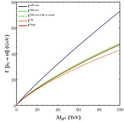
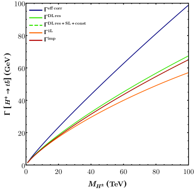
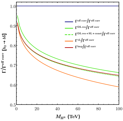
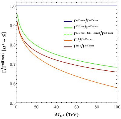
Figure 3: The electroweak corrections to the Higgs decay width into $b\bar{b}$ final states are shown for a ${\cal CP}$-even heavy doublet state (left-hand column). The corresponding plots for the ${\cal CP}$-odd doublet state are virtually identical. The plots in the column on the right-hand side correspond to the charged-Higgs decay $H^{+}\to t\bar{b}$. We display the decay widths in the first row, whereas they are normalized to $\Gamma^{\text{eff}}$ in the second row for a better appreciation of the magnitude of the effects. The blue curve represents the prediction for $\Gamma^{\text{eff}}$, the effective tree-level width including short-distance corrections of SUSY particles as well as long-distance effects from QCD and QED. The green solid curve additionally accounts for the Sudakov double logarithms while the green dashed curve also evaluates the impact of single logarithms and constant terms. The orange curve is the full one-loop evaluation at fixed order obtained from the diagrammatic calculation. For the red curve we combine a resummation of the double logarithms with this full one-loop evaluation, according to Eq. (8). In the case of $H^{+}\to t\bar{b}$, the green dashed curve is hidden by the red one.

Two-body decay width

We first consider the decay width into final states including (anti)quarks of the third generation for heavy doublet-like states in the scenario presented above. In Fig. 3, we plot these decay widths against the mass of the charged Higgs $M_{H^{\pm}}$ (we recall that $M_{H^{\pm}}\approx M_{h_{2}}\approx M_{h_{4}}$) in several approximations. The QCD and QED corrections are included per default, as well as the decoupling SUSY effects. For the blue curve, we only consider the width resulting from this level of approximation (denoted as $\Gamma^{\text{eff corr}}=\Gamma^{\text{eff}}\,\Gamma^{\text{QCD+QED}}/\Gamma^{\text{Born}}$ in the following): this is essentially the popular description employed in public codes such as HDECAY. The green solid curve corresponds to the ‘improved tree-level’ result, where Sudakov double logarithms are included:

$$\Gamma^{\text{DL res}} =\frac{\Gamma^{\text{QCD+QED}}}{\Gamma^{\text{Born}}}\,\Gamma^{\text{eff}}\,\exp{\left(\frac{\Delta\Gamma^{\text{DL}}}{\Gamma^{\text{Born}}}\right)}\,.$$ (15)

The green dashed curve is obtained after additionally incorporating the single logarithms and constant (non-logarithmic) pieces. The result of the full diagrammatic one-loop calculation of Ref. Domingo:2018uim (denoted as $\Gamma^{\text{1L}}=\Gamma^{\text{FO}}\,\Gamma^{\text{QCD+QED}}/\Gamma^{\text{Born}}$ in the following) is displayed in orange. Finally, we show the full one-loop width including resummation of the Sudakov double logarithms ($\Gamma^{\text{imp}}$ of Eq. (8)) in red. In the second row, we show the same estimates normalized to $\Gamma^{\text{eff}}$. The left-hand side focuses on the decay channel $h_{2}\to b\bar{b}$ of the ${\cal CP}$-even doublet-like state $h_{2}$, while the column on the right-hand side considers $H^{+}\to t\bar{b}$. The effects are largely comparable in both cases.

As expected, the impact of the electroweak corrections reaches $\mathcal{O}{\left(10\%\right)}$ for $M_{H^{\pm}}\sim 1$ TeV and more than $40\%$ at $M_{H^{\pm}}\sim 100$ TeV. While the tree-level-improved width, including the resummed double logarithms (green solid curve), gives a good qualitative approximation, it is still $\mathord{\sim}\,5\%$ off as compared to the full result. The agreement can be further refined if we account for the single logarithms and constant terms (green dashed curve; considering only the single logarithms would lead to an approximation of intermediate quality). Obviously, the resummation of Sudakov double logarithms only yields an appreciable effect beyond $M_{H^{\pm}}\operatorname{\raisebox{-3.00003pt}{$\stackrel{{\scriptstyle\displaystyle>}}{{\sim}}$}}10$ TeV, as the red and orange curves remain comparatively close below this mark. It only amounts to $\mathcal{O}{\left(5\text{--}10\%\right)}$ as compared to $\Gamma^{\text{1L}}$ beyond.

Three-body widths

Now, we turn to the three-body decays. In the upper row of Fig. 4, we show the widths of the three-body channels $h_{2}\to W^{-}t\bar{b}$ (left) and $H^{+}\to W^{+}b\bar{b}$ (right) in the same scenario as in Fig. 3. The orange curve corresponds to the full three-body width, while the contribution from on-shell intermediate particles (in particular $t\to W^{+}b$) is shown in green. The resulting genuine three-body contribution (beyond the two-body approximation) is shown in red and corresponds to the piece dominated by Sudakov double logarithms. We observe that this off-shell component (we continue to use this terminology below) is sizable and of competitive magnitude as compared to the two-body widths.

In the lower row of Fig. 4, we display the off-shell component of the three-body widths for the various relevant three-body channels (restricting ourselves to top and bottom quarks in the final state). Their sum is displayed in red. We observe that these contributions roughly reach the magnitude of the electroweak effects in the two-body width, corresponding to the difference between the blue and red curves in Fig. 3. We also stress that the three-body contribution is not of negligible size as compared to the two-body widths, so that we expect a sizable impact at the level of the branching ratios.

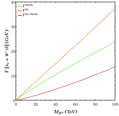
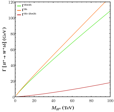
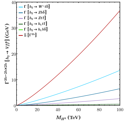
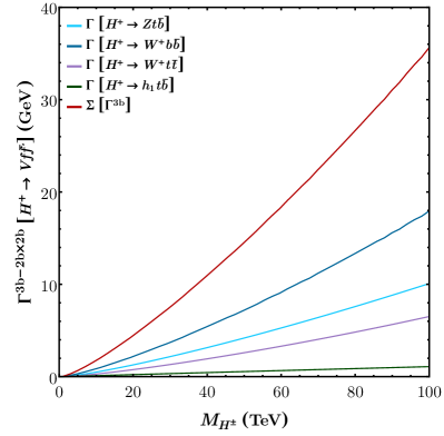
Figure 4: The fermionic three-body decay widths of a heavy decoupling ${\cal CP}$-even doublet (left column) and a charged Higgs (right column) are shown.
Top: the decay widths for the channels $h_{2}\to W^{-}t\bar{b}$ (left) and $H^{+}\to W^{+}b\bar{b}$ (right); we display the full three-body width in orange; in green, we show the two-body contributions mediated by an intermediate on-shell line (in particular $h_{2}\to t(\mbox{$\bar{t}\to W^{-}\bar{b}$})$ and $H^{+}\to(\mbox{$t\to W^{+}b$})\bar{b}$); the red curve corresponds to the genuine three-body contribution beyond the two-body approximation (difference of the orange and green curves).
Bottom: the various three-body contributions beyond the two-body approximation, considering only top and bottom quarks in the final state; the various channels with radiation of a gauge boson are displayed in shades of blue; radiation of a SM-like Higgs boson is shown in shades of green; the red curve corresponds to the sum of all these individual channels.

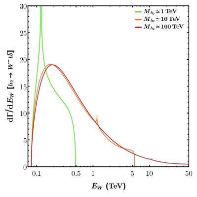
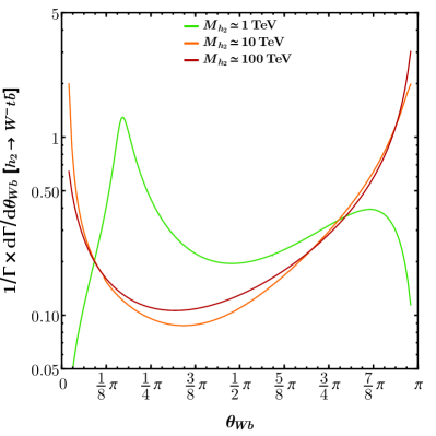
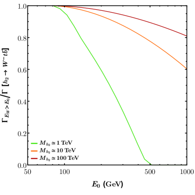
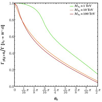
Figure 5: Softness and collinearity of the off-shell contribution to $\Gamma\left[\mbox{$h_{2}\to W^{-}t\bar{b}$}\,\right]$ for $M_{h_{2}}\approx 1$ TeV (green), $10$ TeV (orange) and $100$ TeV (red).
Top left: the differential cross-section in terms of the energy of the $W$ boson in the rest-frame of $h_{2}$ systematically peaks in the lower range of available energy. The apparent spikes slightly above $E_{W}\sim 0.1,1,10$ TeV (depending on the curve) are artifacts of the subtraction of the two-body contribution $h_{2}\to t\left(\mbox{$\bar{t}\to W\bar{b}$}\right)$.
Bottom left: the integrated cross-section as a function of the cutoff on the energy of the radiated $W$ boson.
Top right: the differential cross-section in terms of the angle between the $W$ boson and the $b$ antiquark (in the rest-frame of $h_{2}$) peaks for collinear emissions of $W$ and $\bar{b}$ (at $\theta_{Wb}=0$), or $W$ and $t$, or $b$ and $\bar{t}$ (at $\theta_{Wb}=\pi$).
Bottom right: the fraction of the width captured after requiring a minimal angular separation of $\theta_{0}$ between all the final states falls very rapidly at $\theta_{0}\operatorname{\raisebox{-3.00003pt}{$\stackrel{{\scriptstyle\displaystyle>}}{{\sim}}$}}0$.

From the IR nature of the leading off-shell effects, one can expect the (off-shell) three-body widths to exhibit soft and collinear characteristics. We illustrate this fact in Fig. 5 for the channel $h_{2}\to W^{-}t\bar{b}$, with the three cases $M_{h_{2}}\approx 1$ TeV (green), $10$ TeV (orange) and $100$ TeV (red). The differential cross-section is shown in the upper row, in terms of the energy of the $W$ boson $E_{W}$ (left), and in terms of the angle between the $W$ and the $b$ antiquark $\theta_{Wb}$ (right), in the rest-frame of the Higgs boson. We observe that the differential cross-section peaks at lower values of $E_{W}\sim 100\text{--}200$ GeV as well as at $\theta_{Wb}\sim 0$ (collinear $W$ and $\bar{b}$) or $\pi$ (collinear $W$ and $t$, or collinear $t$ and $\bar{b}$). The visible spikes in the upper-left plot slightly above $E_{W}\sim 0.1,1,10$ TeV for $M_{H^{\pm}}=1,10,100$ TeV are associated to the threshold for the on-shell decay $h_{2}\to t\left(\mbox{$\bar{t}\to W\bar{b}$}\right)$; the corresponding width is subtracted from the three-body width as a Breit–Wigner distribution that, however, does not perfectly match the threshold effect.

In the lower row of Fig. 5, we show how much of the off-shell three-body decay width can be actually observed when requiring a minimal energy of the radiated $W$ (left), or when requiring angular separations of $\theta_{0}\in\left[0,\,\pi/2\right]$ between all the particles in the final state (in the rest-frame of the decaying Higgs; plot on the right): while the width depends only weakly on the energy cutoff as long as the initial state is very heavy, up to $40\%$ of the signal could be lost with an angular cut of $20^{\circ}\approx 0.35$ for $M_{h}\simeq 10\text{--}100$ TeV. Thus, these three-body decays may be experimentally challenging. In particular, the part of the signal that produces collinear pairs with a $W$ boson and a $b$ quark could be misinterpreted as originating in an on-shell $t$. On the other hand, a collinear $t$–$W$ pair is unlikely to be mistaken for an on-shell $b$. The exact boundary between two-body and three-body decays on the experimental side would probably require a dedicated analysis, which goes beyond the scope of this paper.

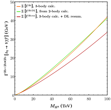
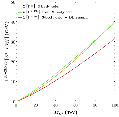
Figure 6: The inclusive three-body width and resummation of double logarithms for a ${\cal CP}$-even doublet-like Higgs (left) and a charged Higgs (right) are shown. The sum of three-body contributions involving fermions of the third generation in the final state from a direct fixed-order calculation (as in Fig. 4, but also including the leptonic channels) is shown in orange. In green, we present the double-logarithmic approximation derived from the Sudakov double logarithms of $h_{2}\to t\bar{t},b\bar{b},\tau^{+}\tau^{-}$; in red, we combine the fixed-order calculation and the resummation of double logarithms.

The impact of the resummation of double logarithms can be observed on Fig. 6. The green curve corresponds to the approximation of the inclusive three-body widths that can be inferred from the Sudakov double logarithms of the two-body channels $h_{2}\to t\bar{t},b\bar{b},\tau^{+}\tau^{-}$ (left) and $H^{+}\to t\bar{b},\tau^{+}\nu_{\tau}$ (right). It is roughly comparable with the result obtained from a direct calculation of the three-body channels (orange curve). The red curve implements Eq. (14). That this curve is somewhat below the green and orange ones can be expected from its definition: if we expand the exponential term in Eq. (14), it is obvious that we are adding a negative contribution from the Sudakov resummation to the widths obtained through explicit calculation.

In these estimates of the three-body widths, we stress that (as our educated guess) the same QCD and QED correction factors as in the two-body widths are applied, in particular with QCD-running Yukawa couplings at the scale of the mass of the decaying Higgs. While these effects are formally of higher order, they have a sizable numerical impact on the widths. At $M_{h_{2}}\approx 100$ TeV for example, the QCD running represents a correction factor of about $1/4$, meaning that, evaluated with ‘pole’ Yukawa couplings, the three-body widths would dominate the two-body channels instead of being comparable. Yet, the QCD$\times$EW order is in principle not under control in our calculation, meaning that the large difference between the widths obtained from ‘pole’ and ‘running’ Yukawa couplings should be interpreted, strictly speaking, as a contribution to the theoretical uncertainty.

Branching ratios

The Higgs branching ratios are often more helpful quantities than the decay widths, as they are more easily accessible experimentally. The three-body decays then affect all decay channels through their intervention in the full Higgs widths. We stress that the final states including the radiation of electroweak gauge bosons and Higgs bosons are clearly distinguishable from the two-body final states and that counting e. g. $W^{-}t\bar{b}$ as a $b\bar{b}$ event is only weakly motivated from an experimental perspective. We thus define the branching fractions as actual ratios of the two-body decay widths by the total width.

We continue to consider the decoupling scenario that has been presented before and show the results in Fig. 7. The following three approximations are displayed: in green, only the QCD/QED-corrected widths $\Gamma^{\text{eff}}$ (together with the factorized SUSY effect) are included, thus dismissing the electroweak corrections; the orange curves are obtained by considering the two-body widths $\Gamma^{\text{imp}}$ at the full one-loop order, but no three-body channel is counted in the total width (thus amounting to an incomplete one-loop result); in red, we add the three-body decay widths in the total width, thus achieving a consistent prediction of the two-body branching fractions at the full one-loop order. In all these evaluations, the fermionic decays are implemented as described in Sect. *, including in particular the resummation of Sudakov double logarithms. In addition, the two-body decays into the gauge bosons of the SM are incorporated at the (improved) one-loop order, as defined in Ref. Domingo:2018uim . The decays involving final states with electroweak gauge bosons are suppressed at the tree level in the decoupling limit, so that corrections of Sudakov type play a negligible part in radiative effects (dominated by the fermion loops). All other two-body decays are included at the tree level, in particular the suppressed $h_{2}\to Vh_{1}$ or $h_{2}\to 2\,h_{1}$ channels (decays into SUSY particles are kinematically forbidden in the scenario under consideration).

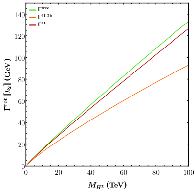
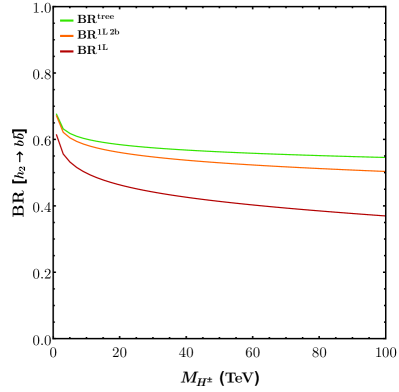
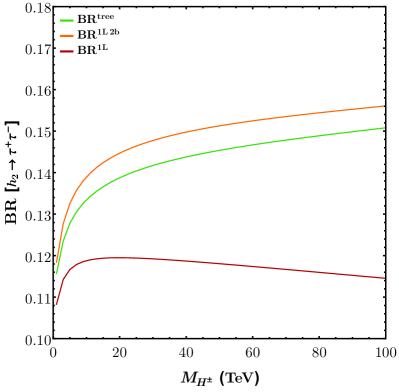
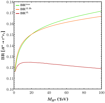
Figure 7: Total width and branching ratios of a heavy doublet-like Higgs states:
Top left: total width of the ${\cal CP}$-even state $h_{2}$ at the (QCD/QED/SUSY-corrected) tree-level order (green), considering only the two-body decays at one-loop order (orange), and including also the three-body decays (red).
Top right: branching ratio of the ${\cal CP}$-even state $h_{2}$ into $b\bar{b}$.
Bottom left: branching ratio of the ${\cal CP}$-even state $h_{2}$ into $\tau^{+}\tau^{-}$.
Bottom right: branching ratio of the charged state $H^{+}$ into $\tau^{+}\nu_{\tau}$.
The branching ratios are derived at the same orders as the total widths, i. e. employing only (QCD/QED/SUSY-corrected) effective widths (green), considering only the two-body decays at the one-loop order (orange), and finally, including also the three-body decays (red).

On the left-hand side of Fig. 7, in the upper row, we first display the total widths of the heavy ${\cal CP}$-even state for the three considered approximations: the one-loop corrections to the two-body decays (orange curve) lead to a suppression of the total width (as compared to the effective tree-level order, in green), consistent with what was observed in Fig. 3, and mainly driven by the Sudakov double logarithms of Eq. (5). Nevertheless, the inclusion of the three-body decays (red) approximately restores the magnitude of the (QCD/QED-corrected) tree-level total width: this is an expected result, due to the cancellation of the double logarithms between the two- and three-body decays. On the right-hand side, we show the branching ratio $\text{BR}{\left[\mbox{$h_{2}\to b\bar{b}$}\,\right]}$, i. e. that of the naively dominant decay channel of the ${\cal CP}$-even state. We observe that this quantity is suppressed, as compared to the tree-level prediction, by the decrease of the two-body width (orange line) but even more so by the inclusion of the three-body decays in the total width (red line). The impact of the one-loop corrections to the two-body decays is only at the percent level, while that of the inclusion of the three-body decays in the total width is of order $\mathord{\sim}\,10\%$ at $M_{h_{2}}\approx 1$ TeV and reaches $\mathord{\sim}\,30\%$ at $M_{h_{2}}\approx 100$ TeV. This can be easily understood when considering that the total width in the strict two-body approximation is suppressed in about the same proportion by the double logarithms as $\Gamma\left[\mbox{$h_{2}\to b\bar{b}$}\,\right]$ (its leading contribution): therefore, we expect little difference between the green and orange curves. On the contrary, when we include the three-body decays, the total width is approximately restored to its effective tree-level value, so that $\text{BR}{\left[\mbox{$h_{2}\to b\bar{b}$}\,\right]}$ becomes sensitive to the suppression of the associated decay width through double logarithms.

In the second row of Fig. 7, we turn to the leptonic decays $h_{2}\to\tau^{+}\tau^{-}$ (left) and $H^{+}\to\tau^{+}\nu_{\tau}$ (right) as the typical search channels at proton–proton colliders. Contrarily to what we observed in the case of $\text{BR}{\left[\mbox{$h_{2}\to b\bar{b}$}\,\right]}$, the prediction for $\text{BR}{\left[\mbox{$h_{2}\to\tau^{+}\tau^{-}$}\right]}$ that is exclusively based on one-loop-corrected two-body widths (orange) is not suppressed, but enhanced. Indeed, in this approximation, the total width, dominated by $h_{2}\to b\bar{b}$, receives a larger suppression as compared to the width of $h_{2}\to\tau^{+}\tau^{-}$: the effect amounts to less than $\mathord{\sim}\,5\%$ depending on $M_{h_{2}}$, and the green and orange curves show the same behavior—and so do they in the case $H^{+}\to\tau^{+}\nu_{\tau}$. However, the estimate at the full one-loop order (i. e. including the three-body decays; in red) shows the opposite trend. Again, as the three-body channels restore the magnitude of the total width to approximately its original effective value, there cannot be an associated enhancement any longer. On the contrary, the branching fractions become sensitive to the suppression of the tau-onic widths via Sudakov effects. Consequently, the discrepancy with the two-body approximation is sizable, loosely amounting to about $10\%$ of the corresponding branching ratio at $M_{h_{2}}\approx 1$ TeV and reaching $\mathord{\sim}\,30\%$ at $M_{h_{2}}\approx 100$ TeV.

This short study shows that it is in fact misleading to assume that the one-loop corrections at the level of the two-body widths are sufficient to provide predictive branching ratios at the full one-loop order. We actually observe little difference with the effective tree-level in this approximation, while the inclusion of the three-body decays generates a sizable shift. []Conclusions

In this paper, we have emphasized the impact of the electroweak radiative corrections on the decays of heavy Higgs states. Focusing on the specific case of fermionic decays in the NMSSM, we have shown that such contributions are dominated by effects of IR type, namely Sudakov double logarithms, which could have a sizable impact on the magnitude of the two-body decay widths. This structure also provides a grasp on the electroweak corrections of higher order, since the leading double logarithms can be explicitly resummed.

In addition, we have stressed the relevance of three-body decay channels for a consistent evaluation of the total widths and branching ratios at the full one-loop order. The IR effects of the two-body widths are indeed mirrored by double logarithms in the radiation of electroweak gauge bosons, whereas the emission of light Higgs bosons only contributes at single-logarithmic order. Contrarily to the radiation of gluons and photons in QCD/QED, the radiation of electroweak gauge bosons leads to clearly distinguishable final states (due to the explicit IR cutoff fulfilled by the mass of the gauge bosons) and, in any case, the definition of an inclusive width is non-trivial (e. g. due to the flavor changes associated to emissions of $W$ bosons). On the other hand, the off-shell three-body signals exhibit the expected soft and collinear characteristics that could make them difficult to extract experimentally.

Numerically, the inclusion of the three-body decays largely compensates the suppression of the two-body widths associated to electroweak effects, resulting in an approximately stable total width when simultaneously including or discarding the electroweak virtual corrections and real emissions. As a consequence, the branching ratios into two-body final states are fully sensitive to the suppression of the two-body widths associated to the double-logarithmic effects. We insist upon our conclusion that an estimation of the total Higgs widths and the branching ratios at the one-loop order solely from the loop-corrected two-body widths fails to capture the actual impact of the electroweak corrections.

In this work, we have focused on final states with SM fermions, since they are the expectedly leading decay channels of heavy doublet-like Higgs bosons involving SM particles in the final state—bosonic decays are suppressed in the decoupling limit. However, the main ingredients that we have discussed here also apply in alternative scenarios, e. g. decays into bosonic or SUSY final states. Indeed, three-body channels always need to be considered in parallel with one-loop corrections for a consistent order-counting and the Sudakov effects are always expected to emerge in electroweak corrections as long as there exists a hierarchy between the mass of the decaying Higgs (center-of-mass energy) and the decay products. However, these effects are only significant if the born-level amplitude itself is unsuppressed. By lowering the scale of the SUSY spectrum such that heavy Higgs bosons can decay into (comparatively) light pairs of neutralinos, charginos or sfermions, we should thus again recover sizable Sudakov corrections and relevant three-body decay widths in these channels with SUSY final states.

References

- (1) ATLAS Collaboration, Phys. Lett. B716, 1 (2012), arXiv:1207.7214.
- (2) CMS Collaboration, Phys. Lett. B716, 30 (2012), arXiv:1207.7235.
- (3) ATLAS Collaboration, CMS Collaboration, Phys. Rev. Lett. 114, 191803 (2015), arXiv:1503.07589.
- (4) E. Bagnaschi, et al., Eur. Phys. J. C79, 617 (2019), arXiv:1808.07542.
- (5) F. Domingo, G. Weiglein, JHEP 04, 095 (2016), arXiv:1509.07283.
- (6) ATLAS Collaboration, CMS Collaboration, JHEP 08, 045 (2016), arXiv:1606.02266.
- (7) CMS Collaboration, A. M. Sirunyan, et al., Eur. Phys. J. C79, 421 (2019), arXiv:1809.10733.
- (8) ATLAS Collaboration, (2019), arXiv:1909.02845.
- (9) V. V. Sudakov, Sov. Phys. JETP 3, 65 (1956), [Zh. Eksp. Teor. Fiz.30,87(1956)].
- (10) J. H. Kühn, A. A. Penin, V. A. Smirnov, Eur. Phys. J. C17, 97 (2000), arXiv:hep-ph/9912503.
- (11) A. Denner, S. Pozzorini, Eur. Phys. J. C18, 461 (2001), arXiv:hep-ph/0010201.
- (12) U. Ellwanger, C. Hugonie, A. Teixeira, Phys. Rept. 496, 1 (2010), arXiv:0910.1785.
- (13) M. Maniatis, Int. J. Mod. Phys. A25, 3505 (2010), arXiv:0906.0777.
- (14) H. Nilles, Phys. Rept. 110, 1 (1984).
- (15) H. Haber, G. Kane, Phys. Rept. 117, 75 (1985).
- (16) J. Kim, H. Nilles, Phys. Lett. B138, 150 (1984).
- (17) U. Ellwanger, M. Rodríguez-Vázquez, JHEP 02, 096 (2016), arXiv:1512.04281.
- (18) E. Conte, B. Fuks, J. Guo, J. Li, A. Williams, JHEP 05, 100 (2016), arXiv:1604.05394.
- (19) M. Guchait, J. Kumar, Phys. Rev. D95, 035036 (2017), arXiv:1608.05693.
- (20) M. Badziak, C. Wagner, JHEP 02, 050 (2017), arXiv:1611.02353.
- (21) S. P. Das, M. Nowakowski, Phys. Rev. D96, 055014 (2017), arXiv:1612.07241.
- (22) J. Cao, X. Guo, Y. He, P. Wu, Y. Zhang, Phys. Rev. D95, 116001 (2017), arXiv:1612.08522.
- (23) B. Das, S. Moretti, S. Munir, P. Poulose, Eur. Phys. J. C77, 544 (2017), arXiv:1704.02941.
- (24) M. Mühlleitner, M. O. P. Sampaio, R. Santos, J. Wittbrodt, JHEP 08, 132 (2017), arXiv:1703.07750.
- (25) U. Ellwanger, A. M. Teixeira, JHEP 10, 113 (2014), arXiv:1406.7221.
- (26) A. Chakraborty, D. K. Ghosh, S. Mondal, S. Poddar, D. Sengupta, Phys. Rev. D91, 115018 (2015), arXiv:1503.07592.
- (27) J. S. Kim, D. Schmeier, J. Tattersall, Phys. Rev. D93, 055018 (2016), arXiv:1510.04871.
- (28) M. Carena, J. Osborne, N. R. Shah, C. E. M. Wagner, Phys. Rev. D98, 115010 (2018), arXiv:1809.11082.
- (29) A. Titterton, U. Ellwanger, H. U. Flächer, S. Moretti, C. H. Shepherd-Themistocleous, JHEP 10, 064 (2018), arXiv:1807.10672.
- (30) J. Cao, Y. He, L. Shang, W. Su, Y. Zhang, JHEP 08, 037 (2016), arXiv:1606.04416.
- (31) Q.-F. Xiang, X.-J. Bi, P.-F. Yin, Z.-H. Yu, Phys. Rev. D94, 055031 (2016), arXiv:1606.02149.
- (32) J. Cao, Y. He, L. Shang, Y. Zhang, P. Zhu, Phys. Rev. D99, 075020 (2019), arXiv:1810.09143.
- (33) U. Ellwanger, C. Hugonie, Eur. Phys. J. C78, 735 (2018), arXiv:1806.09478.
- (34) F. Domingo, J. S. Kim, V. Martin-Lozano, P. Martin-Ramiro, R. Ruiz de Austri, (2018), arXiv:1812.05186.
- (35) U. Ellwanger, J. Gunion, C. Hugonie, JHEP 02, 066 (2005), arXiv:hep-ph/0406215.
- (36) U. Ellwanger, C. Hugonie, Comput. Phys. Commun. 175, 290 (2006), arXiv:hep-ph/0508022.
- (37) F. Domingo, JHEP 06, 052 (2015), arXiv:1503.07087.
- (38) See: www.th.u-psud.fr/NMHDECAY/nmssmtools.html.
- (39) J. Baglio, R. Gröber, M. Mühlleitner, D. Nhung, H. Rzehak, M. Spira, J. Streicher, K. Walz, Comput. Phys. Commun. 185, 3372 (2014), arXiv:1312.4788.
- (40) See: itp.kit.edu/~maggie/NMSSMCALC/.
- (41) A. Djouadi, J. Kalinowski, M. Spira, Comput. Phys. Commun. 108, 56 (1998), arXiv:hep-ph/9704448.
- (42) A. Djouadi, J. Kalinowski, M. Muehlleitner, M. Spira, Comput. Phys. Commun. 238, 214 (2019), arXiv:1801.09506.
- (43) B. Allanach, Comput. Phys. Commun. 143, 305 (2002), arXiv:hep-ph/0104145.
- (44) B. Allanach, P. Athron, L. Tunstall, A. Voigt, A. Williams, Comput. Phys. Commun. 185, 2322 (2014), arXiv:1311.7659.
- (45) B. Allanach, T. Cridge, Comput. Phys. Commun. 220, 417 (2017), arXiv:1703.09717.
- (46) See: code.sloops.free.fr.
- (47) G. Bélanger, V. Bizouard, G. Chalons, Phys. Rev. D89, 095023 (2014), arXiv:1402.3522.
- (48) G. Bélanger, V. Bizouard, F. Boudjema, G. Chalons, Phys. Rev. D93, 115031 (2016), arXiv:1602.05495.
- (49) G. Bélanger, V. Bizouard, F. Boudjema, G. Chalons, Phys. Rev. D96, 015040 (2017), arXiv:1705.02209.
- (50) M. Goodsell, S. Liebler, F. Staub, Eur. Phys. J. C77, 758 (2017), arXiv:1703.09237.
- (51) W. Porod, Comput. Phys. Commun. 153, 275 (2003), arXiv:hep-ph/0301101.
- (52) W. Porod, F. Staub, Comput. Phys. Commun. 183, 2458 (2012), arXiv:1104.1573.
- (53) M. Goodsell, K. Nickel, F. Staub, Eur. Phys. J. C75, 32 (2015), arXiv:1411.0675.
- (54) See: spheno.hepforge.org.
- (55) F. Staub, Comput. Phys. Commun. 181, 1077 (2010), arXiv:0909.2863.
- (56) F. Staub, Comput. Phys. Commun. 182, 808 (2011), arXiv:1002.0840.
- (57) F. Staub, Comput. Phys. Commun. 184, 1792 (2013), arXiv:1207.0906.
- (58) F. Staub, Comput. Phys. Commun. 185, 1773 (2014), arXiv:1309.7223.
- (59) F. Domingo, S. Heinemeyer, S. Paßehr, G. Weiglein, Eur. Phys. J. C78, 942 (2018), arXiv:1807.06322.
- (60) M. Krause, M. Mühlleitner, M. Spira, (2018), arXiv:1810.00768.
- (61) M. Krause, M. Mühlleitner, (2019), arXiv:1904.02103.
- (62) S. Kanemura, M. Kikuchi, K. Mawatari, K. Sakurai, K. Yagyu, (2019), arXiv:1906.10070.
- (63) M. Spira, Prog. Part. Nucl. Phys. 95, 98 (2017), arXiv:1612.07651.
- (64) J. F. Gunion, H. E. Haber, Phys. Rev. D67, 075019 (2003), arXiv:hep-ph/0207010.
- (65) A. Djouadi, J. Kalinowski, P. M. Zerwas, Z. Phys. C70, 435 (1996), arXiv:hep-ph/9511342.
- (66) E. Braaten, J. Leveille, Phys. Rev. D22, 715 (1980).
- (67) M. Drees, K. Hikasa, Phys. Lett. B240, 455 (1990), [Erratum: Phys. Lett. B262, 497 (1991)].
- (68) CMS Collaboration, (2016), CDS 2221747.
- (69) S. Heinemeyer, W. Hollik, G. Weiglein, Eur. Phys. J. C9, 343 (1999), arXiv:hep-ph/9812472.
- (70) S. Heinemeyer, W. Hollik, G. Weiglein, Comput. Phys. Commun. 124, 76 (2000), arXiv:hep-ph/9812320.
- (71) G. Degrassi, S. Heinemeyer, W. Hollik, P. Slavich, G. Weiglein, Eur. Phys. J. C28, 133 (2003), arXiv:hep-ph/0212020.
- (72) M. Frank, T. Hahn, S. Heinemeyer, W. Hollik, H. Rzehak, G. Weiglein, JHEP 0702, 047 (2007), arXiv:hep-ph/0611326.
- (73) T. Hahn, S. Heinemeyer, W. Hollik, H. Rzehak, G. Weiglein, Phys. Rev. Lett. 112, 141801 (2014), arXiv:1312.4937.
- (74) H. Bahl, W. Hollik, Eur. Phys. J. C76, 499 (2016), arXiv:1608.01880.
- (75) H. Bahl, S. Heinemeyer, W. Hollik, G. Weiglein, Eur. Phys. J. C78, 57 (2018), arXiv:1706.00346.
- (76) See: www.feynhiggs.de.
- (77) P. Drechsel, L. Galeta, S. Heinemeyer, G. Weiglein, Eur. Phys. J. C77, 42 (2017), arXiv:1601.08100.
- (78) F. Domingo, P. Drechsel, S. Paßehr, Eur. Phys. J. C77, 562 (2017), arXiv:1706.00437.
- (79) V. S. Fadin, L. N. Lipatov, A. D. Martin, M. Melles, Phys. Rev. D61, 094002 (2000), arXiv:hep-ph/9910338.
- (80) J. Küblbeck, M. Böhm, A. Denner, Comput. Phys. Commun. 60, 165 (1990).
- (81) T. Hahn, Comput. Phys. Commun. 140, 418 (2001), arXiv:hep-ph/0012260.
- (82) T. Hahn, M. Pérez-Victoria, Comput. Phys. Commun. 118, 153 (1999), arXiv:hep-ph/9807565.
- (83) A. Dabelstein, Nucl. Phys. B456, 25 (1995), arXiv:hep-ph/9503443.
- (84) T. Banks, Nucl. Phys. B303, 172 (1988).
- (85) L. Hall, R. Rattazzi, U. Sarid, Phys. Rev. D50, 7048 (1994), arXiv:hep-ph/9306309.
- (86) R. Hempfling, Phys. Rev. D49, 6168 (1994).
- (87) M. Carena, M. Olechowski, S. Pokorski, C. Wagner, Nucl. Phys. B426, 269 (1994), arXiv:hep-ph/9402253.
- (88) M. Carena, D. Garcia, U. Nierste, C. Wagner, Nucl. Phys. B577, 88 (2000), arXiv:hep-ph/9912516.
- (89) H. Eberl, K. Hidaka, S. Kraml, W. Majerotto, Y. Yamada, Phys. Rev. D62, 055006 (2000), arXiv:hep-ph/9912463.
- (90) G. Degrassi, P. Gambino, G. F. Giudice, JHEP 12, 009 (2000), arXiv:hep-ph/0009337.
- (91) A. J. Buras, P. H. Chankowski, J. Rosiek, L. Slawianowska, Nucl. Phys. B659, 3 (2003), arXiv:hep-ph/0210145.
- (92) J. Guasch, P. Hafliger, M. Spira, Phys. Rev. D68, 115001 (2003), arXiv:hep-ph/0305101.
- (93) D. Noth, M. Spira, Phys. Rev. Lett. 101, 181801 (2008), arXiv:0808.0087.
- (94) D. Noth, M. Spira, JHEP 06, 084 (2011), arXiv:1001.1935.
- (95) K. Williams, H. Rzehak, G. Weiglein, Eur. Phys. J. C71, 1669 (2011), arXiv:1103.1335.
- (96) M. Ghezzi, S. Glaus, D. Müller, T. Schmidt, M. Spira, (2017), arXiv:1711.02555.
- (97) A. Djouadi, P. Gambino, Phys. Rev. D51, 218 (1995), arXiv:hep-ph/9406431, [Erratum: Phys. Rev.D53,4111(1996)].