Simulation of 3D elasto-acoustic wave propagation based on a Discontinuous Galerkin Spectral Element method

Abstract

In this paper we present a numerical discretization of the coupled elasto-acoustic wave propagation problem based on a Discontinuous Galerkin Spectral Element (DGSE) approach in a three-dimensional setting. The unknowns of the coupled problem are the displacement field and the velocity potential, in the elastic and the acoustic domains, respectively, thereby resulting in a symmetric formulation. After stating the main theoretical results, we assess the performance of the method by convergence tests carried out on both matching and non-matching grids, and we simulate realistic scenarios where elasto-acoustic coupling occurs. In particular, we consider the case of Scholte waves and the scattering of elastic waves by an underground acoustic cavity. Numerical simulations are carried out by means of the code SPEED, available at http://speed.mox.polimi.it.

MSC2010: 65M12, 65M60, 86A17
Keywords: Discontinuous Galerkin methods, wave propagation, elasto-acoustics, Spectral Elements, computational geophysics, seismic waves, underground cavities

Introduction

The main goal of this work is to simulate three-dimensional scenarios of elasto-acoustic coupling via a Discontinuous Galerkin Spectral Element (DGSE) discretization. Coupled elasto-acoustic wave propagation arises in several scientific and engineering contexts. In a geophysical framework, a first example one can think of is given by seismic events occurring near coastal environments; another relevant situation where such a problem plays a major role is the detection of underground cavities [1, 2, 3]. Elasto-acoustic coupling occurs in structural acoustics as well, when sensing or actuation devices are immersed in an acoustic fluid [4], and also in medical ultrasonics [5, 6].

Typically, an elasto-acoustic coupling arises in the following framework: a space region made up by two subregions, one occupied by a solid (elastic) medium, the other by a fluid (acoustic) one, with suitable transmission conditions imposed at the interface between the two. The aim of such conditions is to account for the following physical properties:  (i) the normal component of the velocity field is continuous at the interface; (ii) a pressure load is exerted by the fluid body on the solid one through the interface. In a geophysics context, when a seismic event occurs near a coastal environment, both pressure (P) and shear (S) waves are generated. However, only P-waves (i.e., whose direction of propagation is aligned with the displacement of the medium) are able to travel through both solid and fluid media, unlike S-waves (i.e., whose direction of propagation is orthogonal to the displacement of the medium), which can travel only through solids. This explains the reason for considering the first interface condition. On the other hand, the second one accounts for the fact that an acoustic wave propagating in a fluid domain gives rise to an acoustic pressure exerted on the solid via the interface.

Numerical simulation of elasto-acoustic coupling scenarios has been the subject of a very broad literature. We give below a brief (and by far non-exhaustive) overview of some of the research works carried out so far in this field. Bathe et al. [7] and Bermúdez et al. [8] considered a displacement-based formulation in both subdomains. Komatitsch et al. [9] introduced a Spectral Element method for modeling wave propagation in media with both fluid (acoustic) and solid (elastic) regions. The employed formulation is symmetric (i.e., it is made in terms of displacement in elastic regions and velocity potential in acoustic regions), and matching between domains is implemented based on an interface integral in the framework of an explicit prediction-multicorrection staggered time scheme. Bermúdez et al. [10] considered a Finite Element approach to the problem based on a pressure formulation in the acoustic domain. Chaljub et al. [11] studied a Spectral Element approach for modeling elastic wave propagation in a solid-fluid sphere by taking into account the local effects of gravity, employing a symmetric formulation, as here. Flemisch et al. [4] devised a numerical treatment based on two independent triangulations on the elastic and acoustic domains with Finite Elements. Due to the flexible construction of both grids, the finite element nodes on the elastic and acoustic boundary on the interface may, in general, not coincide, so as to allow as much flexibility as possible; as a result, non-conforming grids appear at the interface of the two subdomains. Käser and Dumbser [12] considered a numerical scheme suited for unstructured 2D and 3D meshes based on a Discontinuous Galerkin approach to simulate seismic wave propagation in heterogeneous media containing fluid-solid interfaces, using a formulation in terms of a first-order hyperbolic system in velocity-stress unknowns. The solution across element interfaces is handled by Riemann solvers or numerical fluxes. De Basabe and Sen [13] investigated the stability of the Spectral Element method and the Interior Penalty Discontinuous Galerkin method, considering the Lax-Wendroff method for time stepping and showing that it allows for a larger time step than the usual leap-frog finite difference method, with higher-order accuracy. Wilcox et al. [14] studied a high-order Discontinuous Galerkin scheme for the three-dimensional problem based on a velocity-strain formulation, allowing for the solution of the acoustic and elastic wave equations within the same unified framework, based on a first-order system of hyperbolic equations. Soares [15] considered a stabilized time-domain Boundary Element method to discretize each sub-domain. Bottero et al. [16] used a time-domain Spectral Element method for simulations of wave propagation in the framework of ocean acoustics. Terrana et al. [17] studied a high-order hybridizable Discontinuous Galerkin Spectral Element method, again based on a first-order hyperbolic velocity-strain formulation of the wave equations written in conservative form. Very recently, Appelö and Wang [18] devised an energy-based Discontinuous Galerkin approach, again using a symmetric formulation. Finally, a detailed $hp$-convergence analysis of a Discontinuous Galerkin method on polytopal meshes has been presented and validated in a two-dimensional setting in [19], wherein also a well-posedness result has been obtained by a semigroup-based approach.

In this paper, the unknowns of the problem are the displacement field in the solid domain and the velocity potential in the fluid domain, i.e., we employ a symmetric formulation. The latter, say $\varphi$, is defined in terms of the acoustic velocity field $\mathbf{v}_{a}$ in such a way that $\mathbf{v}_{a}=-\bm{\nabla}\varphi$. Also, the acoustic pressure $p_{a}$ in the fluid region is given by $p_{a}=\rho_{a}\accentset{\mbox{\footnotesize.}}{\varphi}$, with $\accentset{\mbox{\footnotesize.}}{\varphi}$ the first time derivative of the velocity potential.

In the context of earthquake ground motion simulations, the numerical scheme employed has to satisfy the following requirements: accuracy, geometric flexibility, and scalability. To be accurate, the numerical method must keep dissipative and dispersive errors low. Geometric flexibility is required since the computational domain usually features complicated geometrical shapes as well as sharp discontinuities of mechanical properties. Finally, real-life seismic scenarios are typically characterized by domains whose dimension, ranging from hundreds to thousands square kilometers, is very large compared with the wavelengths of interest. This typically leads to a discrete problem featuring several millions of unknowns. As a consequence, parallel algorithms must be scalable in order to efficiently exploit high performance computers.

To comply with these requirements, we employ a Discontinuous Galerkin Spectral Element (DGSE) approach based on a domain decomposition paradigm, which was introduced in [20]. More precisely, the discontinuities are imposed only at the interfaces between suitable non-conforming macroregions, so that the flexibility of the DG methods is preserved while keeping the accuracy and efficiency of Spectral Element (SE) methods and avoiding the proliferation of degrees of freedom that characterize DG methods. We refer to [21] for a more detailed and comprehensive review of discretization methods for seismic wave propagation problems.

The rest of the paper is organized as follows. In Section 1 we give the formulation of the problem and recall the well-posedness result proven in [19] under suitable hypotheses on source terms and initial values. In Section 2 we introduce the DGSE method and present the formulation of the semi-discrete problem, also recalling a stability result for its formulation in a suitable energy norm, as well as $hp$-convergence results (with $h$ and $p$ denoting the meshsize and the polynomial approximation degree, respectively) for the error in the same norm; a discussion of the fully discrete formulation of the problem is presented as well. Finally, in Section 3, we present several numerical experiments carried out in a three-dimensional setting, with the two-fold aim of verifying the theoretical results and simulating test cases of physical interest.

Throughout the paper, we will use standard notation for Sobolev spaces [22]. The Sobolev spaces of vector-valued functions are denoted by $\textbf{H}^{m}(\Omega)\equiv[H^{m}(\Omega)]^{d}$ and their norms by $\|{\cdot}\|_{m,\Omega}$, where $\Omega\subset\mathbb{R}^{d}$ is an open bounded domain of $\mathbb{R}^{d}$, $d\in\{2,3\}$. We will use the symbol $(\cdot,\cdot)_{\Omega}$ and $\|{\cdot}\|_{\Omega}$ to denote the standard inner product and norm in the space $H^{0}(\Omega)\equiv L^{2}(\Omega)$, respectively. We also use the abridged notation $x\lesssim y$ in place of $x\leq Cy$, for $C>0$ independent of the discretization parameters (polynomial degree and meshsize), but possibly depending on the material properties of the media under consideration.

1 Problem statement

In this section, we recall the formulation of the elasto-acoustic problem in its symmetric form, i.e., written in terms of the displacement field $\mathbf{u}$ and the velocity potential $\varphi$, defined such that the velocity field in the acoustic domain $\mathbf{v}_{a}$ is given by $\mathbf{v}_{a}=-\bm{\nabla}\varphi$ (see [19]). Let $\Omega\equiv\Omega_{e}\cup\Omega_{a}\subset\mathbb{R}^{3}$ denote an open bounded domain with Lipschitz boundary, given by the union of two open disjoint bounded subdomains $\Omega_{e}$ and $\Omega_{a}$ representing the elastic and acoustic regions in their reference configurations, respectively. We denote by $\Gamma_{\mathrm{I}}\equiv\partial\Omega_{e}\cap\partial\Omega_{a}$ the interface between the two domains. Thus, given a body force $\mathbf{f}_{e}$ and a scalar volume acoustic source $f_{a}$ as well as a final time $T>0$, the strong formulation of the problem reads

$$\left\{\begin{aligned} {\rho_{e}\accentset{\mbox{\footnotesize..}}{\mathbf{u}}-\mathbf{div}\,\bm{\sigma}(\mathbf{u})}&={\mathbf{f}_{e}}&\qquad&\hbox{in }\Omega_{e}\times(0,T],\\[4.0pt] \bm{\sigma}(\mathbf{u})\mathbf{n}_{e}&=-\rho_{a}\accentset{\mbox{\footnotesize.}}{\varphi}\,\mathbf{n}_{e}&\qquad&\hbox{on }\Gamma_{\mathrm{I}}\times(0,T],\\[4.0pt] c^{-2}\accentset{\mbox{\footnotesize..}}{\varphi}-\triangle\varphi&=f_{a}&\qquad&\hbox{in }\Omega_{a}\times(0,T],\\[4.0pt] {\partial\varphi}/{\partial\mathbf{n}_{a}}&=-\accentset{\mbox{\footnotesize.}}{\mathbf{u}}\raisebox{-0.86108pt}{\scalebox{1.3}{$\cdot$}}\mathbf{n}_{a}&\qquad&\hbox{on }\Gamma_{\mathrm{I}}\times(0,T],\\[4.0pt] \end{aligned}$$

coupled with suitable boundary and initial conditions that are detailed below.

Here, $\rho_{e}\in L^{\infty}(\Omega_{e})$, $\rho_{e}>0$, is the mass density of the elastic region $\Omega_{e}$; $\bm{\sigma}(\mathbf{u})=\mathbb{C}\bm{\varepsilon}(\mathbf{u})=\lambda(\mbox{\rm tr}\,\bm{\varepsilon}(\mathbf{u}))\mathbf{I}+2\mu\bm{\varepsilon}(\mathbf{u})$ is the Cauchy stress tensor; $\mathbb{C}$ is the uniformly elliptic and symmetric fourth-order elasticity tensor, representing a linearly elastic isotropic behavior, with $\mu$ and $\lambda$ the Lamé parameters; $\bm{\varepsilon}(\mathbf{u})=\mbox{\rm sym}\,(\bm{\nabla}\mathbf{u})=\frac{1}{2}\left(\bm{\nabla}\mathbf{u}+\bm{\nabla}\mathbf{u}^{T}\right)$ is the strain tensor. Also, we denote by $\rho_{a}\in L^{\infty}(\Omega_{a})$, $\rho_{a}>0$, the density of the acoustic region $\Omega_{a}$ and by $c>0$ the speed of the acoustic wave.

The trasmission conditions on $\Gamma_{\mathrm{I}}$ take account of the pressure, of magnitude $\rho_{a}|\accentset{\mbox{\footnotesize.}}{\varphi}|$, exterted by the acoustic region onto the elastic one through the interface, and of the continuity of the normal component of the velocity field at the interface.

Concerning boundary conditions we assume the following decomposition: $\partial\Omega=(\partial\Omega_{e}\cup\partial\Omega_{a})\setminus\Gamma_{\mathrm{I}}$ where $\partial\Omega_{e}=\Gamma_{e,D}\cup\Gamma_{e,N}\cup\Gamma_{e,N\!R}\cup\Gamma_{\mathrm{I}}$ and $\partial\Omega_{a}=\Gamma_{a,D}\cup\Gamma_{a,N}\cup\Gamma_{a,N\!R}\cup\Gamma_{\mathrm{I}}$. We denote by $\mathbf{n}_{e}$ and $\mathbf{n}_{a}$ the outer unit normal vectors to $\partial\Omega_{e}$ and $\partial\Omega_{a}$, respectively. Homogeneous Dirichlet boundary conditions are assigned on $\Gamma_{e,D}\cup\Gamma_{a,D}$, i.e., $\mathbf{u}=\mathbf{0}$ and $\varphi=0$. Neumann boundary conditions on $\Gamma_{e,N}\cup\Gamma_{a,N}$ are prescribed in term of a surface traction $\mathbf{g}_{e}$ and a surface acoustic flux $g_{a}$ as

$$\left\{\begin{aligned} \bm{\sigma}(\mathbf{u})\mathbf{n}_{e}&=\mathbf{g}_{e}&\qquad&\hbox{on }\Gamma_{e,N}\times(0,T],\\ {\partial\varphi}/{\partial\mathbf{n}_{a}}&=g_{a}&\qquad&\hbox{on }\Gamma_{a,N}\times(0,T].\\ \end{aligned}\right.$$

Non-reflecting boundary conditions are imposed on $\Gamma_{e,N\!R}\cup\Gamma_{a,N\!R}$; here, the surface loads are themselves expressed in terms of the time derivatives of the unknowns. In particular, we set

$$\left\{\begin{aligned} \bm{\sigma}(\mathbf{u})\mathbf{n}_{e}&=\mathbf{g}_{e}^{\star}&\qquad&\hbox{on }\Gamma_{e,{N\!R}}\times(0,T],\\ {\partial\varphi}/{\partial\mathbf{n}_{a}}&=g_{a}^{\star}&\qquad&\hbox{on }\Gamma_{a,{N\!R}}\times(0,T],\\ \end{aligned}\right.$$ (1)

with $\mathbf{g}_{e}^{\star}\equiv\rho_{e}c_{P}(\accentset{\mbox{\footnotesize.}}{\mathbf{u}}\cdot\mathbf{n}_{e})\mathbf{n}_{e}+\rho_{e}c_{S}\accentset{\mbox{\footnotesize.}}{\mathbf{u}}_{\tau}$ and $g_{a}^{\star}\equiv c^{-1}\accentset{\mbox{\footnotesize.}}{\varphi}$ (see e.g. [23, 24, 4]), with $\accentset{\mbox{\footnotesize.}}{\mathbf{u}}_{\tau}\equiv\accentset{\mbox{\footnotesize.}}{\mathbf{u}}-(\accentset{\mbox{\footnotesize.}}{\mathbf{u}}\cdot\mathbf{n}_{e})\mathbf{n}_{e}$ is the tangential velocity field over $\Gamma_{e,N\!R}$, and $c_{P}$ and $c_{S}$ are the propagation velocities of P (pressure) and S (shear) waves, respectively, given by $c_{P}=\sqrt{{(\lambda+2\mu)}/{\rho_{e}}}$ and $c_{S}=\sqrt{{\mu}/{\rho_{e}}}$. These are commonly referred to in literature as first order absorbing boundaries [25].

Finally, as initial conditions we set $\mathbf{u}(\cdot,0)=\mathbf{u}_{0}$ and $\accentset{\mbox{\footnotesize.}}{\mathbf{u}}(\cdot,0)=\mathbf{u}_{1}$ in $\Omega_{e}$ while $\varphi(\cdot,0)=\varphi_{0}$ and $\accentset{\mbox{\footnotesize.}}{\varphi}(\cdot,0)=\varphi_{1}$ in $\Omega_{a}$, for some regular enough functions ${\mathbf{u}_{0}},{\mathbf{u}_{1}},\varphi_{0}$, and $\varphi_{1}$.

The well-posedness of the problem (1) in suitable functional spaces was proven in [19] under suitable regularity assumptions on the data, in the case $\Gamma_{e,N}\cup\Gamma_{a,N}=\emptyset=\Gamma_{e,N\!R}\cup\Gamma_{a,N\!R}$.

2 Numerical discretization

In this section we present the numerical approximation of the weak formulation of (1) through a DGSE method coupled with an explicit Newmark predictor-corrector staggered time marching scheme (see [9]). We first introduce the semi-discrete counterpart of (1), observing that the solution of (1) satisfies the following weak form: for any $t\in(0,T]$, and all $(\mathbf{v},\psi)\in{\mathbf{H}^{1}_{\Gamma_{e,D}}(\Omega_{e})}\times{H^{1}_{\Gamma_{a,D}}(\Omega_{a})}$,

$$\begin{multlined}(\rho_{e}\accentset{\mbox{\footnotesize..}}{\mathbf{u}}(t),\mathbf{v})_{\Omega_{e}}+(c^{-2}\rho_{a}\accentset{\mbox{\footnotesize..}}{\varphi}(t),\psi)_{\Omega_{a}}+\mathcal{A}_{e}(\mathbf{u}(t),\mathbf{v})+\mathcal{A}_{a}(\varphi(t),\psi)+\mathcal{I}_{e}(\accentset{\mbox{\footnotesize.}}{\varphi}(t),\mathbf{v})+\mathcal{I}_{a}(\accentset{\mbox{\footnotesize.}}{\mathbf{u}}(t),\psi)\\[2.0pt] =({\mathbf{f}_{e}}(t),\mathbf{v})_{\Omega_{e}}+(\mathbf{g}_{e}(t),\mathbf{v})_{\Gamma_{e,N}}+(\mathbf{g}_{e}^{\star}(t),\mathbf{v})_{\Gamma_{e,N\!R}}\\ +(f_{a}(t),\psi)_{\Omega_{a}}+(g_{a}(t),\psi)_{\Gamma_{a,N}}+(\mathbf{g}_{a}^{\star}(t),\mathbf{v})_{\Gamma_{a,N\!R}},\end{multlined}(\rho_{e}\accentset{\mbox{\footnotesize..}}{\mathbf{u}}(t),\mathbf{v})_{\Omega_{e}}+(c^{-2}\rho_{a}\accentset{\mbox{\footnotesize..}}{\varphi}(t),\psi)_{\Omega_{a}}+\mathcal{A}_{e}(\mathbf{u}(t),\mathbf{v})+\mathcal{A}_{a}(\varphi(t),\psi)+\mathcal{I}_{e}(\accentset{\mbox{\footnotesize.}}{\varphi}(t),\mathbf{v})+\mathcal{I}_{a}(\accentset{\mbox{\footnotesize.}}{\mathbf{u}}(t),\psi)\\[2.0pt] =({\mathbf{f}_{e}}(t),\mathbf{v})_{\Omega_{e}}+(\mathbf{g}_{e}(t),\mathbf{v})_{\Gamma_{e,N}}+(\mathbf{g}_{e}^{\star}(t),\mathbf{v})_{\Gamma_{e,N\!R}}\\ +(f_{a}(t),\psi)_{\Omega_{a}}+(g_{a}(t),\psi)_{\Gamma_{a,N}}+(\mathbf{g}_{a}^{\star}(t),\mathbf{v})_{\Gamma_{a,N\!R}},$$ (5)

where

$$\begin{aligned} \mathcal{A}_{e}(\mathbf{u},\mathbf{v})&=({\mathbb{C}}\bm{\varepsilon}(\mathbf{u}),\bm{\varepsilon}(\mathbf{v}))_{\Omega_{e}},\\ \mathcal{A}_{a}(\varphi,\psi)&=(\rho_{a}\bm{\nabla}\varphi,\bm{\nabla}\psi)_{\Omega_{a}},\end{aligned}$$

We observe that the second evolution equation has been multiplied by $\rho_{a}$ to ensure (skew)symmetry of the two interface terms (since $\mathbf{n}_{a}=-\mathbf{n}_{e}$).

2.1 Partitions and trace operators

We now consider a decomposition $\mathcal{T}_{\Omega_{e}}$ of $\Omega_{e}$ into $L_{e}$ nonoverlapping polyhedral regions $\Omega_{e}^{\ell}$, $\ell\in\{1,\dots,L_{e}\}$, such that $\Omega_{e}=\bigcup_{\ell=1}^{L_{e}}\Omega_{e}^{\ell}$, with $\Omega_{e}^{\ell}\cap\Omega_{e}^{\ell^{\prime}}=\emptyset$ for any $\ell\neq\ell^{\prime}$. This first macropartition is introduced to distinguish elastic materials with different properties (density $\rho_{e}$ and material moduli $\lambda,\mu$). On each $\Omega_{e}^{\ell}$, we build a conforming computational mesh $\mathcal{T}_{h_{\ell}}^{e}$ of meshsize $h_{\ell}>0$ made of disjoint elements $\mathcal{K}_{e,\ell}$, and suppose that each $\mathcal{K}_{e,\ell}\subset\Omega_{e}^{\ell}$ is the image through an invertible bilinear map $F_{e,\ell}:\widehat{\mathcal{K}}\to\mathcal{K}_{e,\ell}$ of the unit reference hexahedron $\widehat{\mathcal{K}}=(-1,1)^{d}$, $d\in\{2,3\}$. Given two adjacent regions $\Omega_{e}^{\ell^{\pm}}$, we define an internal face $F$ as the non-empty interior of $\partial\overline{{\mathcal{K}}_{e,\ell^{+}}}\cap\partial\overline{{\mathcal{K}}_{e,\ell^{-}}}$, for ${\mathcal{K}}_{e,\ell^{\pm}}\in{\mathcal{T}}_{h_{\ell^{\pm}}}^{e}$, ${\mathcal{K}}_{e,\ell^{\pm}}\subset\Omega_{e}^{\ell^{\pm}}$, and collect all the internal faces in the set $\mathcal{F}_{h,e}^{i}$. Moreover, we define $\mathcal{F}_{h,e}^{D}$, $\mathcal{F}_{h,e}^{N}$, and $\mathcal{F}_{h,e}^{N\!R}$ as the sets of all boundary faces where displacement, tractions, or non-reflecting elastic boundary conditions are imposed, respectively. We collect all the boundary faces not laying on $\Gamma_{\mathrm{I}}$ in the set $\mathcal{F}_{h,e}^{b}$.

On the other hand, concerning the acoustic domain $\Omega_{a}$, since we do not take into account multi-phase fluids, we introduce a conforming grid $\mathcal{T}_{h}^{a}$ of $\Omega_{a}$ made by disjoint hexahedral elements $\mathcal{K}_{a}$. As in the elastic case, we suppose that each $\mathcal{K}_{e,\ell}\subset\Omega_{e}^{\ell}$ is the image through an invertible bilinear map $F_{a}:\widehat{\mathcal{K}}\to\mathcal{K}_{a}$ of the unit reference hexahedron $\widehat{\mathcal{K}}=(-1,1)^{d}$, $d\in\{2,3\}$. Also, we define $\mathcal{F}_{h,a}^{D}$, $\mathcal{F}_{h,a}^{N}$, and $\mathcal{F}_{h,a}^{N\!R}$ as the sets of all boundary faces where velocity potential, fluxes, or non-reflecting acoustic boundary conditions are imposed, respectively. We collect all the boundary faces not laying on $\Gamma_{\mathrm{I}}$ in the set $\mathcal{F}_{h,a}^{b}$.

Finally, we collect all faces laying on $\Gamma_{\mathrm{I}}$ in the set $\mathcal{F}_{h,\Gamma_{\mathrm{I}}}$; in this case, $F\in\mathcal{F}_{h,\Gamma_{\mathrm{I}}}$ is the non-empty interior of $\partial\overline{{\mathcal{K}}_{e,\ell}}\cap\partial\overline{{\mathcal{K}}_{a}}$, for given ${\mathcal{K}}_{e,\ell}\subset\Omega_{e}^{\ell}\in\mathcal{T}_{\Omega_{e}}$ and ${\mathcal{K}}_{a}\in\mathcal{T}_{h}^{a}$. Implicit in these definitions is the assumption that each face laying on $\partial\Omega_{e}\cup\partial\Omega_{a}$ can belong to exactly one of the sets $\mathcal{F}_{h,e}^{D}$, $\mathcal{F}_{h,e}^{N}$, $\mathcal{F}_{h,a}^{D}$, $\mathcal{F}_{h,a}^{N}$, and $\mathcal{F}_{h,\Gamma_{\mathrm{I}}}$.

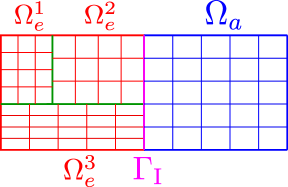
Figure 1: Example of decompositions for the domains $\Omega_{e}$ and $\Omega_{a}$. Interfaces between elastic regions $\Omega_{e}^{1}$, $\Omega_{e}^{2}$, and $\Omega_{e}^{3}$, characterized by different material properties, are highlighted in green, and the elasto-acoustic interface $\Gamma_{\mathrm{I}}$ is highlighted in purple.

Remark 2.1 (Non-matching grids at the elasto-acoustic interface).

Notice that the above-detailed framework allows to handle the situation of non-matching grids at the interface $\Gamma_{\mathrm{I}}$ between the elastic and the acoustic domains (cf. Figure 1). Meshes can therefore be generated independently on each of the domains.

We now introduce the following average and jump operators [26, 27] for mesh faces in the elastic domain. For sufficiently smooth scalar, vector, and tensor fields $\psi$, $\mathbf{v}$, and $\bm{\tau}$, we define averages and jumps on an internal face $F\in\mathcal{F}_{h,e}^{i}$, $F\subset\partial\mathcal{K}_{e,\ell^{+}}\cap\partial\mathcal{K}_{e,\ell^{-}}$, with $\mathcal{K}_{e,\ell^{\pm}}\in\mathcal{T}_{h_{\ell^{\pm}}}^{e}$, as follows:

$${[[{\psi}]]} =\psi^{+}\mathbf{n}^{+}+\psi^{-}\mathbf{n}^{-}, \qquad{\{\{{\psi}\}\}} =\frac{\psi^{+}+\psi^{-}}{2},$$

$${[[{\mathbf{v}}]]} =\mathbf{v}^{+}\otimes\mathbf{n}^{+}+\mathbf{v}^{-}\otimes\mathbf{n}^{-}, \qquad{\{\{{\mathbf{v}}\}\}} =\frac{\mathbf{v}^{+}+\mathbf{v}^{-}}{2},$$

$${[[{\bm{\tau}}]]} =\bm{\tau}^{+}\mathbf{n}^{+}+\bm{\tau}^{-}\mathbf{n}^{-}, \qquad{\{\{{\bm{\tau}}\}\}} =\frac{\bm{\tau}^{+}+\bm{\tau}^{-}}{2},$$

where $\mathbf{a}\otimes\mathbf{b}$ denotes the tensor product of $\mathbf{a},\mathbf{b}\in\mathbb{R}^{3}$; $\psi^{\pm}$, $\mathbf{v}^{\pm}$ and $\bm{\tau}^{\pm}$ are the traces of $\psi$, $\mathbf{v}$ and $\bm{\tau}$ on $F$ taken from the interior of $\mathcal{K}_{e,\ell^{\pm}}$, and $\mathbf{n}^{\pm}$ is the outer unit normal vector to $\partial\mathcal{K}_{e,\ell^{\pm}}$. When considering a boundary face $F\in\mathcal{F}_{h,e}^{b}$, we set ${[[{\psi}]]}=\psi\mathbf{n}$, ${[[{\mathbf{v}}]]}=\mathbf{v}\otimes\mathbf{n}$, ${[[{\bm{\tau}}]]}=\bm{\tau}\mathbf{n}$, and ${\{\{{\psi}\}\}}=\psi$, ${\{\{{\mathbf{v}}\}\}}=\mathbf{v}$, ${\{\{{\bm{\tau}}\}\}}=\bm{\tau}$. We also use the shorthand notation

$$\left\langle\Phi,\Psi\right\rangle_{\mathcal{F}}=\sum_{F\in\mathcal{F}}(\Phi,\Psi)_{F},\qquad\|\Phi\|_{\mathcal{F}}=\left\langle\Phi,\Phi\right\rangle_{\mathcal{F}}^{\nicefrac{{1}}{{2}}},$$

for scalar, vector or tensor fields $\Phi$ and $\Psi$ and for a given generic collection $\mathcal{F}$ of mesh faces.

2.2 Discontinuous Galerkin Spectral Element approximation

First, concerning the elastic domain $\Omega_{e}$, we associate with each subdomain $\Omega_{e}^{\ell}$ a nonnegative integer ${N_{e,\ell}\geq 1}$, and introduce the finite-dimensional space

$$\mathbf{V}(\Omega_{e}^{\ell})=\{\mathbf{v}\in\mathbf{C}^{0}(\overline{\Omega}_{e}^{\ell}):\mathbf{v}_{|\mathcal{K}_{e,\ell}}\circ F_{e,\ell}\in[\mathbb{Q}^{{N_{e,\ell}}}(\widehat{\mathcal{K}})]^{d}\ \forall\mathcal{K}_{e,\ell}\in{\mathcal{T}}_{h_{\ell}}^{e}\},$$ (6)

where $\mathbb{Q}^{{N_{e,\ell}}}(\widehat{\mathcal{K}})$ is the space of polynomials of degree $N_{e,\ell}$ in each coordinate direction on the unit reference hexahedron $\widehat{\mathcal{K}}$. We then introduce the space $\mathbf{V}(\Omega_{e})=\bigtimes_{\ell=1}^{L_{e}}\mathbf{V}(\Omega_{e}^{\ell})$. Concerning the acoustic domain $\Omega_{a}$ we choose a spectral degree $N_{a}\geq 1$ and define the following space:

$${V(\Omega_{a})=\{\psi\in C^{0}(\overline{\Omega}_{a}):\psi_{|\mathcal{K}_{a}}\circ F_{a}\in\mathbb{Q}^{{N_{a}}}(\widehat{\mathcal{K}})\ \forall\mathcal{K}_{a}\in{\mathcal{T}}_{h}^{a}\}.}$$ (7)

The semi-discrete DGSE approximation of (5) reads then: $(\mathbf{u}_{h},\varphi_{h})\!\in\!C^{2}([0,T];\!{\mathbf{V}(\Omega_{e})})\times C^{2}([0,T];\!{V(\Omega_{a}))}$ such that, for all $(\mathbf{v}_{h},\psi_{h})\in{\mathbf{V}(\Omega_{e})}\times{V(\Omega_{a})}$,

$$\begin{multlined}(\rho_{e}\accentset{\mbox{\footnotesize..}}{\mathbf{u}}_{h}(t),\mathbf{v}_{h})_{\Omega_{e}}+(c^{-2}\rho_{a}\accentset{\mbox{\footnotesize..}}{\varphi}_{h}(t),\psi_{h})_{\Omega_{a}}+\mathcal{A}_{h}^{e}(\mathbf{u}_{h}(t),\mathbf{v}_{h})+\mathcal{A}_{h}^{a}(\varphi_{h}(t),\psi_{h})\\[5.0pt] +\mathcal{I}_{h}^{e}(\accentset{\mbox{\footnotesize.}}{\varphi}_{h}(t),\mathbf{v}_{h})+\mathcal{I}_{h}^{a}(\accentset{\mbox{\footnotesize.}}{\mathbf{u}}_{h}(t),\psi_{h})=\mathcal{L}^{e}_{h}(\mathbf{v}_{h})+\mathcal{L}^{a}_{h}(\psi_{h}),\end{multlined}(\rho_{e}\accentset{\mbox{\footnotesize..}}{\mathbf{u}}_{h}(t),\mathbf{v}_{h})_{\Omega_{e}}+(c^{-2}\rho_{a}\accentset{\mbox{\footnotesize..}}{\varphi}_{h}(t),\psi_{h})_{\Omega_{a}}+\mathcal{A}_{h}^{e}(\mathbf{u}_{h}(t),\mathbf{v}_{h})+\mathcal{A}_{h}^{a}(\varphi_{h}(t),\psi_{h})\\[5.0pt] +\mathcal{I}_{h}^{e}(\accentset{\mbox{\footnotesize.}}{\varphi}_{h}(t),\mathbf{v}_{h})+\mathcal{I}_{h}^{a}(\accentset{\mbox{\footnotesize.}}{\mathbf{u}}_{h}(t),\psi_{h})=\mathcal{L}^{e}_{h}(\mathbf{v}_{h})+\mathcal{L}^{a}_{h}(\psi_{h}),$$ (10)

with initial conditions $\left(\mathbf{u}_{h}(0),\accentset{\mbox{\footnotesize.}}{\mathbf{u}}_{h}(0)\right)=\left(\mathbf{u}_{0,h},\mathbf{u}_{1,h}\right)\in{{\mathbf{V}}(\Omega_{e})}\times{{\mathbf{V}}(\Omega_{e})}$, and $\left(\varphi_{h}(0),\accentset{\mbox{\footnotesize.}}{\varphi}_{h}(0)\right)=\left(\varphi_{0,h},\varphi_{1,h}\right)\in{{V}(\Omega_{a})}\times{{V}(\Omega_{a})}$, where $\mathbf{u}_{0,h},\mathbf{u}_{1,h},\varphi_{0,h},\text{ and }\varphi_{1,h}$ are suitable approximations of the initial data. In (10)

$$\mathcal{A}_{h}^{e}(\mathbf{u},\mathbf{v}) =\sum_{\Omega_{e}^{\ell}\in\mathcal{T}_{\Omega_{e}}}(\bm{\sigma}_{h}(\mathbf{u}),\bm{\varepsilon}_{h}(\mathbf{v}))_{\Omega_{e}^{\ell}}-\left\langle{\{\{{\bm{\sigma}_{h}(\mathbf{u})}\}\}},{[[{\mathbf{v}}]]}\right\rangle_{{\mathcal{F}}_{h,e}^{i}}$$ (11)

$$\ \ \ -\left\langle{[[{\mathbf{u}}]]},{\{\{{\bm{\sigma}_{h}(\mathbf{v})}\}\}}\right\rangle_{{\mathcal{F}}_{h,e}^{i}}+\left\langle\eta{[[{\mathbf{u}}]]},{[[{\mathbf{v}}]]}\right\rangle_{{\mathcal{F}}_{h,e}^{i}} \forall\mathbf{u},\mathbf{v}\in{{\mathbf{V}}(\Omega_{e})},$$

$$\mathcal{A}_{h}^{a}(\varphi,\psi) =\sum_{\mathcal{K}_{a}\in\mathcal{T}_{h}^{a}}(\rho_{a}\bm{\nabla}\varphi,\bm{\nabla}\psi)_{\mathcal{K}_{a}} \forall\varphi,\psi\in{V(\Omega_{a})},$$

$$\mathcal{I}_{h}^{e}(\psi,\mathbf{v}) =\left\langle\rho_{a}\psi\mathbf{n}_{e},\mathbf{v}\right\rangle_{\mathcal{F}_{h,\Gamma_{\mathrm{I}}}} \forall(\psi,\mathbf{v})\in{V(\Omega_{a})}\times{{\mathbf{V}}(\Omega_{e})},$$

$$\mathcal{I}_{h}^{a}(\mathbf{v},\psi) =\left\langle{\rho_{a}\mathbf{v}}\raisebox{-0.86108pt}{\scalebox{1.3}{$\cdot$}}{\mathbf{n}_{a}},\psi\right\rangle_{\mathcal{F}_{h,\Gamma_{\mathrm{I}}}}\equiv-\mathcal{I}_{h}^{e}(\psi,\mathbf{v}) \forall(\mathbf{v},\psi)\in{{\mathbf{V}}(\Omega_{e})}\times{V(\Omega_{a})},$$

$$\mathcal{L}^{e}_{h}(\mathbf{v}) =\sum_{\Omega_{e}^{\ell}\in\mathcal{T}_{\Omega_{e}}}(\mathbf{f}_{e}(t),\mathbf{v})_{\Omega_{e}^{\ell}}+\left\langle\mathbf{g}_{e}(t),\mathbf{v}\right\rangle_{\mathcal{F}_{h,e}^{N}}+\left\langle\mathbf{g}_{e}^{\star}(t),\mathbf{v}\right\rangle_{\mathcal{F}_{h,e}^{N\!R}} \forall\mathbf{v}\in{{\mathbf{V}}(\Omega_{e})},$$

$$\mathcal{L}^{a}_{h}(\psi) =\sum_{\mathcal{K}_{a}\in\mathcal{T}_{h}^{a}}(f_{a}(t),\psi)_{\mathcal{K}_{a}}+\left\langle g_{a}(t),\psi\right\rangle_{\mathcal{F}_{h,a}^{N}}+\left\langle g_{a}^{\star}(t),\psi\right\rangle_{\mathcal{F}_{h,a}^{N\!R}} \forall\psi\in{V(\Omega_{a})}.$$

We point out that the fourth identity in (11) holds since $\mathbf{n}_{a}=-\mathbf{n}_{e}$ on $\Gamma_{\mathrm{I}}$. Here we have set, for any $\mathbf{v}\in{{\mathbf{V}}(\Omega_{e})}$,

$$\bm{\varepsilon}_{h}(\mathbf{v})=\frac{1}{2}\left(\bm{\nabla}_{h}\mathbf{v}+\bm{\nabla}_{h}\mathbf{v}^{T}\right),\quad\bm{\sigma}_{h}(\mathbf{v})=\mathbb{C}\bm{\varepsilon}_{h}(\mathbf{v}),$$

with $\bm{\nabla}_{h}$ the usual broken gradient operator. The discontinuity penalization function $\eta\colon\mathcal{F}_{h,e}^{i}\to\mathbb{R}$ is defined as follows:

$$\eta_{|F}=\alpha\{(\lambda+2\mu)^{\pm}\}_{\mathrm{H}}\left\{\left(\frac{N_{e,\ell}^{2}}{h_{\ell}}\right)^{\pm}\right\}_{\mathrm{H}},\quad F\in{\mathcal{F}_{h,e}^{i}},\;F\subset\partial{\mathcal{K}_{e,\ell^{+}}}\cap\partial{\mathcal{K}_{e,\ell^{-}}},$$ (12)

with $\mathcal{K}_{e,\ell^{\pm}}\in\mathcal{T}_{h_{\ell^{\pm}}}^{e}$. Here, $\alpha>0$ is a positive constant to be properly chosen, and $\{v^{\pm}\}_{\mathrm{H}}=2v^{+}v^{-}/(v^{+}+v^{-})$ is the harmonic mean of traces $v^{+}$ and $v^{-}$ of a given scalar field $v$.

Upon introducing the following norms

$$\|\mathbf{v}\|_{{\mathrm{DG}},e}^{2} =\|\mathbb{C}^{\nicefrac{{1}}{{2}}}\bm{\varepsilon}_{h}(\mathbf{v})\|_{\Omega_{e}}^{2}+\|{\eta^{\nicefrac{{1}}{{2}}}{[[{\mathbf{v}}]]}}\|_{{\mathcal{F}_{h,e}^{i}}}^{2} \forall\mathbf{v}\in{{\mathbf{V}}(\Omega_{e})},$$ (13)

$$\|\mathbf{v}(t)\|_{{\mathcal{E}}_{e}}^{2} =\|\rho_{e}^{\nicefrac{{1}}{{2}}}\accentset{\mbox{\footnotesize.}}{\mathbf{v}}(t)\|_{\Omega_{e}}^{2}+\|\rho_{e}^{\nicefrac{{1}}{{2}}}\zeta\mathbf{v}(t)\|_{\Omega_{e}}^{2}+\|\mathbf{v}(t)\|_{{\mathrm{DG}},e}^{2} \forall\mathbf{v}\in C^{1}([0,T];{\mathbf{V}(\Omega_{e})}),$$

$$\|\psi(t)\|_{{\mathcal{E}}_{a}}^{2} =\|c^{-1}\rho_{a}^{\nicefrac{{1}}{{2}}}\accentset{\mbox{\footnotesize.}}{\psi}(t)\|_{\Omega_{a}}^{2}+\|\rho_{a}^{\nicefrac{{1}}{{2}}}\bm{\nabla}\psi(t)\|_{\Omega_{a}}^{2} \forall\psi\in C^{1}([0,T];{V(\Omega_{a})}),$$

it is possible to prove that bilinear forms $\mathcal{A}_{h}^{e}$ and $\mathcal{A}_{h}^{a}$ are continuous and coercive. Consequently, a stability result and an error estimate in the above-defined energy norm for the semi-discrete solution can be inferred. We recall those results below; for the sake of readibility, we give a simplified statement of the error estimate (see [19] for a more general framework, and [28] for the purely elastic case).

Theorem 2.2 (Stability of the semi-discrete formulation).

Let $(\mathbf{u}_{h},\varphi_{h})$ be the solution of (10). For a sufficiently large penalty parameter $\alpha$ in (12), the following bound holds:

$$\|\mathbf{u}_{h}(t)\|_{{\mathcal{E}}_{e}}+\|\varphi_{h}(t)\|_{{\mathcal{E}}_{a}}\lesssim\|\mathbf{u}_{h}(0)\|_{{\mathcal{E}}_{e}}+\|\varphi_{h}(0)\|_{{\mathcal{E}}_{a}}+\int_{0}^{t}\left(\|{\mathbf{f}_{e}}(\tau)\|_{\Omega_{e}}+\|f_{a}(\tau)\|_{\Omega_{a}}\right)\,\mathrm{d}\tau,\quad t\in(0,T].$$ (14)

Theorem 2.3 (A priori error estimate in the energy norm).

Assume that the exact solution of problem (1) is such that $\mathbf{u}\in C^{2}([0,T];\mathbf{H}^{m}(\Omega_{e}))$ and $\varphi\in C^{2}([0,T];H^{n}(\Omega_{a}))$, for given integers $m,n\geq 2$. Then, the following error estimate holds:

$$\sup_{t\in[0,T]}(\|\mathbf{u}_{h}(t)-\mathbf{u}(t)\|_{{\mathcal{E}}_{e}}^{2}+\|\varphi_{h}(t)-\varphi(t)\|_{{\mathcal{E}}_{a}}^{2})\\ \lesssim\sup_{t\in[0,T]}\left(\sum_{\ell=1}^{L_{e}}\frac{h_{\ell}^{2\min(m,N_{e,\ell}+1)-2}}{N_{e,\ell}^{2m-3}}\left(\|\accentset{\mbox{\footnotesize.}}{\mathbf{u}}\|_{m,\Omega_{e}^{\ell}}^{2}+\|\mathbf{u}\|_{m,\Omega_{e}^{\ell}}^{2}\right)\!+\!\sum_{{\mathcal{K}}\in\mathcal{T}_{h}^{a}}\!\!\frac{h_{\mathcal{K}}^{2\min(n,N_{a}+1)-2}}{N_{a,}^{2n-3}}\left(\|\accentset{\mbox{\footnotesize.}}{\varphi}\|_{n,\mathcal{K}}^{2}+\|\varphi\|_{n,\mathcal{K}}^{2}\right)\right)\\ +\int_{0}^{T}\!\left(\sum_{\ell=1}^{L_{e}}\frac{h_{\ell}^{2\min(m,N_{e,\ell}+1)-2}}{N_{e,\ell}^{2m-3}}\left(\|\accentset{\mbox{\footnotesize..}}{\mathbf{u}}\|_{m,\Omega_{e}^{\ell}}^{2}+\|\accentset{\mbox{\footnotesize.}}{\mathbf{u}}\|_{m,\Omega_{e}^{\ell}}^{2}+\|\mathbf{u}\|_{m,\Omega_{e}^{\ell}}^{2}\right)\right.\\ \left.+\sum_{{\mathcal{K}}\in\mathcal{T}_{h}^{a}}\!\!\frac{h_{\mathcal{K}}^{2\min(n,N_{a,}+1)-2}}{N_{a}^{2n-3}}\left(\|\accentset{\mbox{\footnotesize..}}{\varphi}\|_{n,\mathcal{K}}^{2}+\|\accentset{\mbox{\footnotesize.}}{\varphi}\|_{n,\mathcal{K}}^{2}+\|\varphi\|_{n,\mathcal{K}}^{2}\right)\right)\mathrm{d}\tau.$$

Remark 2.4 (Error in the energy norm).

If both meshsizes are quasi-uniform, i.e. $h_{\ell}\simeq h_{e}\ \forall\ell\in\{1,\dots,L_{e}\}$ and $h_{\mathcal{K}}\simeq h_{a}\ \forall\mathcal{K}\in\mathcal{T}_{h}^{a}$, if the polynomial degree is uniform over elastic regions $\Omega_{e}^{\ell}$, i.e. $N_{e,\ell}=N_{e}\ \forall\ell\in\{1,\dots,L_{e}\}$, and if $m\geq N_{e}+1$ and $n\geq N_{a}+1$, the following error estimate holds:

$$\sup_{t\in[0,T]}(\|\mathbf{u}_{h}(t)-\mathbf{u}(t)\|_{{\mathcal{E}}_{e}}+\|\varphi_{h}(t)-\varphi(t)\|_{{\mathcal{E}}_{a}})\lesssim\ {C_{\mathbf{u}}(T)\frac{h_{e}^{N_{e}}}{N_{e}^{m-\nicefrac{{3}}{{2}}}}}+{C_{\varphi}(T)\frac{h_{a}^{N_{a}}}{N_{a}^{n-\nicefrac{{3}}{{2}}}}},$$ (19)

where $C_{\mathbf{u}}(T)$ and $C_{\varphi}(T)$ are positive numbers depending on the final time $T$ and the exact solution, along with its time derivatives.

2.3 Fully discrete formulation

Upon fixing polynomial bases for discrete spaces ${\mathbf{V}(\Omega_{e})}$ and ${V(\Omega_{a})}$, see e.g. [19], the semi-discrete algebraic formulation of problem (10) reads

$$\begin{dcases}\begin{aligned} \mathsf{M}_{e}\accentset{\mbox{\footnotesize..}}{\mathsf{u}}(t)+\mathsf{S}_{e}\accentset{\mbox{\footnotesize.}}{\mathsf{u}}(t)+\mathsf{K}_{e}\mathsf{u}(t)+\mathsf{C}_{e}\accentset{\mbox{\footnotesize.}}{\mathsf{\upphi}}(t)&=\mathsf{f}_{e}(t),\quad t\in(0,T],\\ \mathsf{M}_{a}\accentset{\mbox{\footnotesize..}}{\mathsf{\upphi}}(t)+\mathsf{S}_{a}\accentset{\mbox{\footnotesize.}}{\mathsf{\upphi}}(t)+\mathsf{K}_{a}\mathsf{\upphi}(t)+\mathsf{C}_{a}\accentset{\mbox{\footnotesize.}}{\mathsf{u}}(t)&=\mathsf{f}_{a}(t),\quad t\in(0,T],\end{aligned}\end{dcases}$$ (20)

with initial conditions $\mathsf{u}(0)=\mathsf{u}^{0},\,\accentset{\mbox{\footnotesize.}}{\mathsf{u}}(0)=\mathsf{v}^{0},\,\mathsf{\upphi}(0)=\mathsf{\upphi}^{0}$, and $\accentset{\mbox{\footnotesize.}}{\mathsf{\upphi}}(0)=\mathsf{\uppsi}^{0}$, and where the vectors $\mathsf{u}(t)$ and $\mathsf{\upphi}(t)$ represent the expansion coefficients of $\bm{u}_{h}(t)$ and $\varphi_{h}(t)$ in the chosen bases, respectively. Analogously, $\mathsf{M}_{e}$, $\mathsf{K}_{e}$, and $\mathsf{C}_{e}$ are the matrix representations of the bilinear forms $(\rho_{e}\mathbf{u},\mathbf{v})_{\Omega_{e}},\ \mathcal{A}_{h}(\mathbf{u},\mathbf{v})$ and $\mathcal{I}_{h}^{e}(\psi,\mathbf{v})$, respectively (see (11)). When elastic absorbing boundary conditions are included in the model, matrix $\mathsf{S}_{e}$ takes account of the boundary term $(\mathbf{g}_{e}^{\star},\mathbf{v})_{\Gamma_{e,N\!R}}$; otherwise, it is identically equal to zero. On the other hand, $\mathsf{M}_{a}$, $\mathsf{K}_{a}$, and $\mathsf{C}_{a}\equiv-\mathsf{C}_{e}^{\mathsf{T}}$ represent the bilinear forms $(c^{-2}\rho_{a}\varphi,\psi)_{\Omega_{a}},\ \mathcal{A}_{h}^{a}(\varphi,\psi)$, and $\mathcal{I}_{h}^{a}(\mathbf{v},\psi)$, respectively. When acoustic absorbing boundary conditions are considered, $\mathsf{S}_{a}$ represents the boundary term $(g_{a}^{\star},\psi)_{\Gamma_{a,N\!R}}$. Finally, $\mathsf{f}_{e}(t)$ and $\mathsf{f}_{a}(t)$ are the vector representations of linear functionals $\mathcal{L}_{h}^{e}$ and $\mathcal{L}_{h}^{a}$, respectively.

For the time integration of system (20), as in [9], we employ an explicit Newmark predictor-corrector staggered method [29]; in this case, the scheme is conditionally stable and second-order accurate. We thus subdivide the time interval $[0,T]$ into $N_{T}$ subintervals of amplitude $\Delta t=T/N_{T}$ and denote by $\mathsf{u}^{n}\approx\mathsf{u}(t_{n})$, $\mathsf{v}^{n}\approx\accentset{\mbox{\footnotesize.}}{\mathsf{u}}(t_{n})$, $\mathsf{a}_{e}^{n}\approx\accentset{\mbox{\footnotesize..}}{\mathsf{u}}(t_{n})$, $\mathsf{\upphi}^{n}\approx\mathsf{\upphi}(t_{n})$, $\mathsf{\uppsi}^{n}\approx\accentset{\mbox{\footnotesize.}}{\mathsf{\Phi}}(t_{n})$, and $\mathsf{a}_{a}^{n}\approx\accentset{\mbox{\footnotesize..}}{\mathsf{\upphi}}(t_{n})$ the approximations of $\mathsf{u}$, $\accentset{\mbox{\footnotesize.}}{\mathsf{u}}$, $\accentset{\mbox{\footnotesize..}}{\mathsf{u}}$, $\mathsf{\upphi}$, $\accentset{\mbox{\footnotesize.}}{\mathsf{\upphi}}$, and $\accentset{\mbox{\footnotesize..}}{\mathsf{\upphi}}$ at time $t_{n}=n\Delta t$, $n\in\{0,\dots,N_{T}\}$, respectively. Then, along the lines of [9], we exploit the fact that mass matrices are diagonal, and implement an iterative scheme based on a staggered prediction/correction technique. At each time step, we first compute predictors of the solution in both domains:

$$\widetilde{\mathsf{u}}^{n+1} =\mathsf{u}^{n}+\Delta t\mathsf{v}^{n}+\frac{\Delta t^{2}}{2}\mathsf{a}_{e}^{n}, \widetilde{\mathsf{v}}^{n+1} =\mathsf{v}^{n}+\frac{\Delta t}{2}\mathsf{a}_{e}^{n},$$ (21)

$$\widetilde{\mathsf{\upphi}}^{n+1} =\mathsf{\upphi}^{n}+\Delta t\mathsf{\uppsi}^{n}+\frac{\Delta t^{2}}{2}\mathsf{a}_{a}^{n}, \widetilde{\mathsf{\uppsi}}^{n+1} =\mathsf{\uppsi}^{n}+\frac{\Delta t}{2}\mathsf{a}_{a}^{n}.$$

Then, we update the solution in the elastic domain by solving the first equation of (20) for $\mathsf{a}_{e}^{n+1}$, where the coupling term is evaluated as $-\mathsf{C}_{e}\widetilde{\uppsi}^{n+1}$, hence using the predictor computed in the acoustic domain. Next, we compute the solution in the acoustic domain by solving the second equation of (20) for $\mathsf{a}_{a}^{n+1}$, now using the updated solution in the elastic domain to evaluate the coupling term, which is thus given by $-\mathsf{C}_{a}\mathsf{v}^{n+1}$, where $\mathsf{v}^{n+1}=\widetilde{\mathsf{v}}^{n+1}+\frac{\Delta t}{2}\mathsf{a}_{e}^{n+1}$. We then iterate this algorithm by returning to the first step, this time using the updated solution. The algorithm is summarized in the following scheme.

3 Numerical results

3.1 Verification test

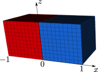
(a) $h=h_{e}=h_{a}=0.1$

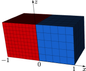
(b) $h_{e}=0.1$, $h_{a}=0.2$

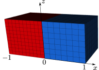
(c) $h_{e}=0.1$, $h_{a}=0.15$

Figure 2: Test case 3.1. Computational domain with matching (a) and non-matching (b)–(c) hexahedral meshes.

In this section we solve problem (1) in the parallelepiped $\Omega=(-1,1)\times(0,1)\times(0,1)$ on both matching and non-matching grids (Figure 2), and verify the convergence results shown in Theorem 2.3. Here $\Omega_{e}=(-1,0)\times(0,1)\times(0,1)$ and $\Omega_{a}=(0,1)^{3}$; the interface is thus given by $\Gamma_{\mathrm{I}}=\{0\}\times[0,1]\times[0,1]$. In all cases we compute the energy norm of the error at time $t=0.1$, cf. (19). For the time discretization we employed the staggered scheme presented in the previous section. The timestep will be precised depending on the case under consideration. Finally, we choose $\rho_{e}=2.7$, $c_{P}=6.20$, $c_{S}=3.12$, $\rho_{a}=1$, and $c=1$ (cf. [5, 6]). The right-hand sides $\mathbf{f}_{e}$ and $f_{a}$ are chosen so that the exact solution is given by

$$\mathbf{u}(x,y,z;t) =\left(\cos\Big{(}\frac{4\pi x}{c_{P}}\Big{)},\,\cos\Big{(}\frac{4\pi x}{c_{S}}\Big{)},\,\cos\Big{(}\frac{4\pi x}{c_{S}}\Big{)}\right)\cos(4\pi t),$$ (22)

$$\varphi(x,y,z;t) =\sin\Big{(}\frac{4\pi x}{c}\Big{)}\sin(4\pi t).$$

Grids are sequentially refined starting from an initial mesh with uniform meshsize $h=0.1$ in the matching case (Figure 2a); on the other hand, in the non-matching case (Figure 2b–2c), the submeshes of $\Omega_{e}$ and $\Omega_{a}$ have the two initial respective meshsizes $h_{e}=0.1$ and $h_{a}=0.2$. Numerical tests carried out in both matching (Figure 4) and non-matching (Figure 4) cases, show that $h$- and $N$-convergence rates match those predicted by (19). We also considered a further non-matching grid, where the initial submeshes are such that their meshsizes are not a multiple of each other, i.e., $h_{e}=0.1$ and $h_{a}=0.15$ (Figure 4c). In this case, we obtain a quadratic order of convergence, as expected with polynomial degree $N_{e}=N_{a}=2$.

3.2 Scholte waves

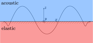
Figure 5: Test case 3.2. Scholte wave at the interface between an elastic medium and an acoustic one.

Scholte waves are an example of boundary waves, propagating along elasto-acoustic interfaces (cf. Figure 5). Their amplitude decays exponentially away from the interface. As in [14], we consider here two half-spaces. The lower half, $z<0$, is occupied by an elastic medium with $\lambda=\mu=1$ and $\rho_{e}=1$; and the upper half, $z>0$, by an acoustic medium with $c=1$ and $\rho_{a}=1$. The analytic expressions of the displacement field $\mathbf{u}\equiv(u_{1},u_{2},u_{3})$ and velocity potential $\varphi$ can be inferred from [14], where a displacement-based formulation is employed in both domains (see also [30, Section 5.2]), and are the following. For $z<0$ (elastic region), we have

$$u_{1}(x,y,z;t) =k(B_{2}e^{kb_{2p}z}-B_{3}b_{2s}e^{kb_{2s}z})\cos(kx-\omega t),$$ (23)

$$u_{2}(x,y,z;t) =0,$$

$$u_{3}(x,y,z;t) =k(B_{2}b_{2p}e^{kb_{2p}z}-B_{3}e^{kb_{2s}z})\sin(kx-\omega t);$$

and, for $z>0$ (acoustic region),

$$\varphi(x,y,z;t)=\omega B_{1}e^{-kb_{1p}z}\cos(kx-\omega t).$$ (24)

Here, the wavenumber is $k=\omega/c_{\mathrm{sch}}$, for a given frequency $\omega$ and Scholte wave speed $c_{\mathrm{sch}}$. The decay rates are given by

$$b_{1p}=\sqrt{1-\frac{c_{\mathrm{sch}}^{2}}{c^{2}}},\qquad b_{2p}=\sqrt{1-\frac{c_{\mathrm{sch}}^{2}}{c_{P}^{2}}},\qquad b_{2s}=\sqrt{1-\frac{c_{\mathrm{sch}}^{2}}{c_{S}^{2}}}.$$

Wave amplitudes $B_{1}$, $B_{2}$, and $B_{3}$ have to satisfy a suitable eigenvalue problem, say $\bm{\Lambda}\mathbf{B}=\mathbf{0}$ with $\bm{\Lambda}$ a suitable $3\times 3$ matrix and $\mathbf{B}\equiv[B_{1}\,\,B_{2}\,\,B_{3}]^{T}$, stemming from the transmission conditions imposed on $\Gamma_{\mathrm{I}}$, i.e. $\bm{\sigma}(\mathbf{u})\mathbf{n}_{e}=-\rho_{a}\accentset{\mbox{\footnotesize.}}{\varphi}\mathbf{n}_{e}$ and $\partial\varphi/\partial\mathbf{n}_{a}=-\accentset{\mbox{\footnotesize.}}{\mathbf{u}}\raisebox{-0.86108pt}{\scalebox{1.3}{$\cdot$}}\mathbf{n}_{a}$. The value of the Scholte wave speed $c_{\mathrm{sch}}$ is thus given by the condition $\det\bm{\Lambda}=0$. One can show that a Scholte wave speed exists for arbitrary combinations of material parameters. Based on the values of the material parameters we selected, we obtain, analogously to [14], $c_{\mathrm{sch}}=0.7110017230197$, and we choose $B_{1}=0.3594499773037$, $B_{2}=0.8194642725978$, and $B_{3}=1$. Also, for our numerical experiments, we choose $\omega=1$, which gives, in turn, $k=1.4064663525$.

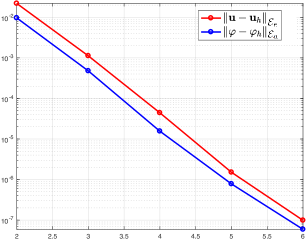
(a)

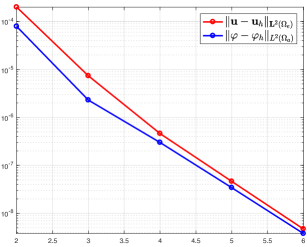
(b)

Figure 6: Test case 3.2. Error in the energy (a) and $L^{2}$ (b) norms vs. $N$ at $t=0.1\,s$, with $N$ ranging from 2 to 6.

We use a uniform mesh consisting of 2400 elements (corresponding to a meshsize $h=h_{e}=h_{a}=0.416$) over the domain $(-1,1)\times(-1,1)\times(-20,20)$, and we impose Dirichlet conditions all over the boundary. Figure 6 shows asymptotic exponential convergence rate of the error in the energy and $L^{2}$ norms, as expected.

3.3 Underground acoustic cavity

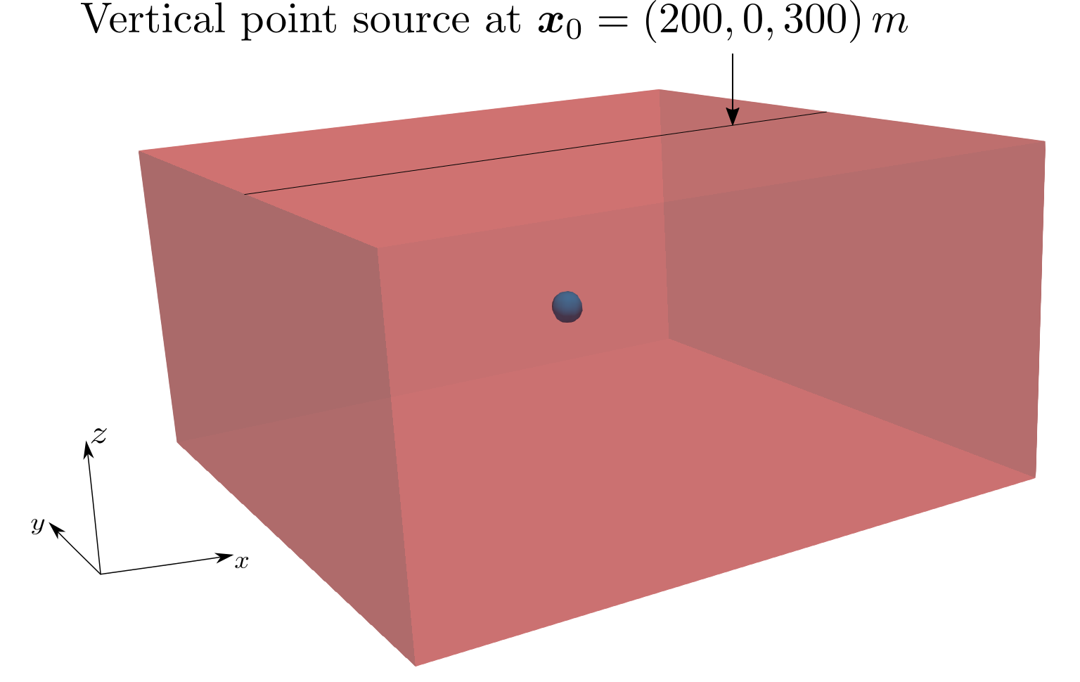
Figure 7: Test case 3.3. Geometry of the computational domain for the case of a seismic wave in the presence of an underground cavity.

As a last test case, we simulate a seismic wave in the presence of an underground spherical acoustic cavity. This problem arises in several applications, the most important one, besides non-destructive testing [31], is given by near-surface seismic studies to detect the presence of cavities in the subsoil, which are originated after underground nuclear explosions, and can give rise to resonance effects when a seismic event occurs [3]. In particular, the geometry we consider is the following: the acoustic domain is given by an open ball $\Omega_{a}=\{\bm{x}\in\mathbb{R}^{3}:\|\bm{x}\|<R\}$, of radius $R=30\,m$, and the elastic one is $\Omega_{e}=(-L_{x},L_{x})\times(-L_{y},L_{y})\times(-L_{z},L_{z})\setminus\overline{\Omega}_{a}$ surrounding the cavity, with $L_{x}=L_{y}=600\,m$ and $L_{z}=300\,m$ (Figure 7). Non-reflecting boundary conditions are imposed on the external elastic boundary. The system is excited by a point Ricker wavelet of the following form:

$$\mathbf{f}_{e}(\bm{x},t)=f(t)\mathbf{e}_{z}\delta(\bm{x}-\bm{x}_{0}),\quad f(t)=f_{0}\left(1-2\pi^{2}f_{p}^{2}(t-t_{0})^{2}\right)e^{-\pi^{2}f_{p}^{2}(t-t_{0})^{2}},$$

with $\mathbf{e}_{z}=(0,0,1)$, $\bm{x}_{0}=(200,0,300)\,m$, $t_{0}=0.25\,s$, $f_{0}=10^{10}\,N$, and peak frequency $f_{p}$. The set of data and space discretization parameters is summarized in Table 1, where we write $c_{P}$ for $c$ in the case of an acoustic wave.

Table 1: Test case 3.3. Material properties.

Region	$\rho_{e/a}\,(kg/m^{3})$	$c_{P}\,(m/s)$	$c_{S}\,(m/s)$
${\Omega_{e}}$	${2700}$	${3000}$	${1734}$
${\Omega_{a}}$	${1024}$	${300}$	–

Since the wavelength inside the cavity is much smaller than outside, we are led to choosing a finer meshsize inside the cavity, and thus employ the following meshsizes: $h_{e}=20\,m$, $h_{a}=5\,m$. We use a polynomial degree $N_{e}=N_{a}=4$ on both domains, and we set the time-step to $\Delta t=10^{-5}\,s$.

Figure 8 shows the $z$-component $u_{z}$ of the displacement field in the subsoil and the acoustic velocity potential $\varphi$ in the spherical cavity at times $t=0.4\,s$, $t=0.5\,s$, and $t=0.7\,s$ when the peak frequency is set to $f_{p}=22\,Hz$, whereas Figure 9 shows the same quantities when $f_{p}=11\,Hz$. We remark that, in the first case (Figure 8), the elastic wave detects the acoustic cavity: spherical wavefronts are generated due to refraction phenomena between the cavity and the subsoil, since the wavelength corresponding to the value $f_{p}=22\,Hz$ is comparable with the diameter of the cavity. On the other hand, if the peak frequency is reduced by a factor two (Figure 9), we observe that the interaction of the elastic wave with the cavity is weaker than in the first case, since the corresponding wavelength is twice as much as in the first case. In both cases, since outside the sphere the material is stiff, the acoustic wave remains trapped within the cavity over time and it generates reflection and refraction effects. These phenomena can be better represented and remarked if the time histories of a number of monitored points in the elastic and acoustic domains are considered. In particular, we took into account an $X$-shaped set of points in a square cross section of the computational domain lying in the $xz$-plane, centered in the origin, with side $600\,m$ (Figure 10). Time histories of points in the subsoil and in the underground cavity are showcased in Figures 11 and 12 for the first case ($f_{p}=22\,Hz$) and in Figures 13 and 14 for the second case ($f_{p}=11\,Hz$). In particular, reflection phenomena for elastic waves are clearly more remarkable in the first case than in the second. As expected, point A being the closest one to the location of the seismic source, is the first to undergo a displacement impulse, which is then delayed for the other points; the same occurs in the second case. Finally, in both cases, we clearly see that the acoustic wave remains trapped in cavity over time, due to persistent reflections.

4 Conclusions and perspectives

We have presented a Discontinuous Galerkin Spectral Element method for the approximation of the elasto-acoustic evolution problem. Several numerical experiments carried out in a three-dimensional framework have been discussed, both to verify the theoretical results and to simulate a scenario of physical interest. Our approach is well-suited to comply with the requirements for the discretization of heterogeneous seismic wave propagation problems (geometric flexibility, high-order accuracy, and flexibility); in addition, it allows for the treatment of non-matching grids at the interface between the elastic and the acoustic domains, which can therefore be generated independently on each of the domains. All numerical experiments have been carried out using the computer code SPEED [23], freely available at http://speed.mox.polimi.it.

A future work consists in the extension to general polyhedral meshes in SPEED, in order to tame the computational cost of mesh generation and enhance the geometrical flexibility of the numerical discretization. As a second perspective is given by the enrichment of the models.

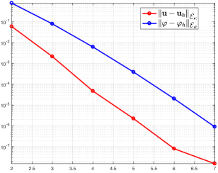
(c) $N=N_{e}=N_{a}$ ranging from 2 to 7

Figure 3: Test case 3.1. Error in the energy norm vs. $h$ (a)–(b) and $N$ (c) at $t=0.1\,s$.

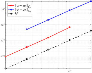
(a) $N=N_{e}=N_{a}=2$

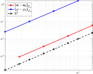
(c) $N=N_{e}=N_{a}=2$

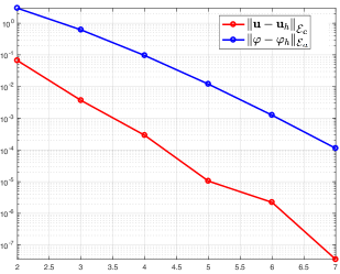
(d) $h_{e}=0.1$, $h_{a}=0.2$, $N$ ranging from 2 to 7

Figure 4: Test case 3.1. Error error vs. $h$ (a)–(b)–(c) and $N$ (d) at $t=0.1\,s$ for non-matching hexahedral grids. Initial meshsizes are $h_{e}=0.1$, $h_{a}=0.2$ in (a) and (b), and $h_{e}=0.1$, $h_{a}=0.15$ in (c).

(a)

(b)

(c)

Figure 8: Test case 3.3. Displacement along the $z$-direction and velocity potential at time $t=0.4\,s$ (a), $t=0.5\,s$ (b), and $t=0.7\,s$ (c), for $f_{p}=22\,Hz$.

(a)

(b)

(c)

Figure 9: Test case 3.3. Displacement along the $z$-direction and velocity potential at time $t=0.4\,s$ (a), $t=0.5\,s$ (b), and $t=0.7\,s$ (c), for $f_{p}=11\,Hz$.

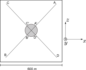
Figure 10: Test case 3.3. Set of monitors in the square cross section of the computational domain lying in the $xz$-plane, centered in the origin, with side $600\,m$.

(a)

(b)

Figure 11: Test case 3.3. Time histories of the displacement along the $z$-direction for the monitored points in the elastic subsoil, for $f_{p}=22\,Hz$.

(a)

(b)

Figure 12: Test case 3.3. Time histories of the velocity potential for the monitored points in the acoustic cavity, for $f_{p}=22\,Hz$.

(a)

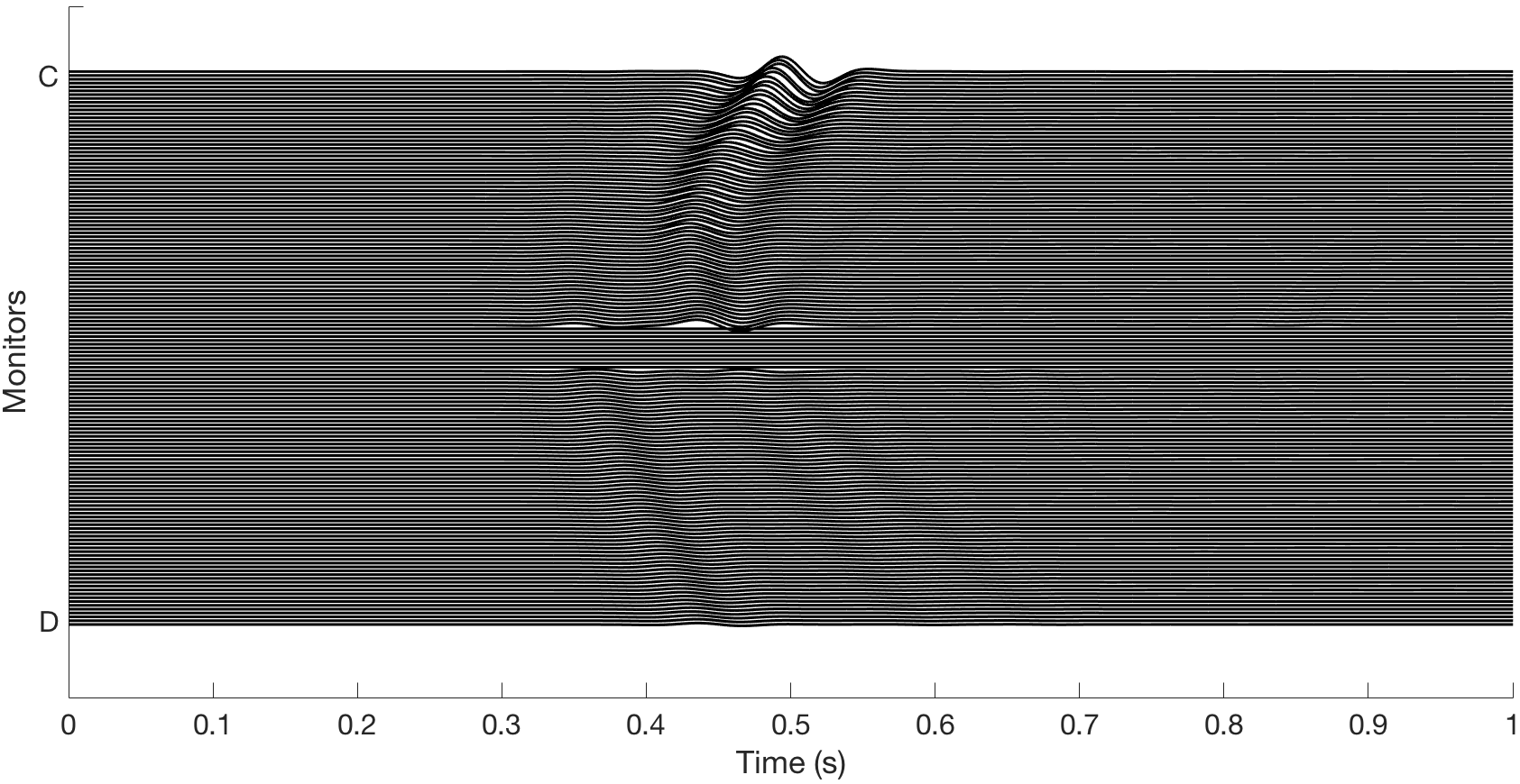
(b)

Figure 13: Test case 3.3. Time histories of the displacement along the $z$-direction for the monitored points in the elastic subsoil, for $f_{p}=11\,Hz$.

(a)

(b)

Figure 14: Test case 3.3. Time histories of the velocity potential for the monitored points in the acoustic cavity, for $f_{p}=11\,Hz$.

References

- [1] S. Esterhazy, F. Schneider, I. Mazzieri, and G. Bokelmann. Insights into the modeling of seismic waves for the detection of underground cavities. Technical Report 67/2017, MOX, Politecnico di Milano, 2017.
- [2] S. Esterhazy, F. Schneider, I. Perugia, and G. Bokelmann. Application of high-order finite-element method to the p-wave propagation around and inside an underground cavity. Geophysics, 82:T197–T206, 2017.
- [3] F. Schneider, S. Esterhazy, I. Perugia, and G. Bokelmann. Seismic resonances of spherical acoustic cavities. Geophysical Prospecting, 65:1–24, 2017.
- [4] B. Flemisch, M. Kaltenbacher, and B. I. Wohlmuth. Elasto–acoustic and acoustic–acoustic coupling on non-matching grids. Int. J. Numer. Meth. Engng, 67:1791–1810, 2006.
- [5] S. Mönköla. Numerical simulation of fluid-structure interaction between acoustic and elastic waves. PhD thesis, University of Jyväskylä, 2011.
- [6] S. Mönköla. On the accuracy and efficiency of transient spectral element models for seismic wave problems. Adv. Math. Phys., 2016.
- [7] K. J. Bathe, C. Nitikitpaiboon, and X. Wang. A mixed displacement-based finite element formulation for acoustic fluid-structure interaction. Computers & Structures, 56:225–237, 1995.
- [8] A. Bermúdez, L. Hervella-Nieto, and R. Rodríguez. Finite element computation of three-dimensional elastoacoustic vibrations. Journal of Sound and Vibration, 219:279–306, 1999.
- [9] D. Komatitsch, C. Barnes, and J. Tromp. Wave propagation near a fluid-solid interface: a spectral-element approach. Geophysics, 65:623–631, 2000.
- [10] A. Bermúdez, P. Gamallo, L. Hervella-Nieto, and R. Rodríguez. Finite element analysis of pressure formulation of the elastoacoustic problem. Numer. Math., 95:29–51, 2003.
- [11] E. Chaljub, Y. Capdeville, and J. P. Vilotte. Solving elastodynamics in a fluid-solid heterogeneous sphere: a parallel spectral element approximation on non-conforming grids. J. Comput. Phys., 187:457–491, 2003.
- [12] M. Käser and M. Dumbser. A highly accurate discontinuous galerkin method for complex interfaces between solids and moving fluids. Geophysics, 73:T23–T35, 2008.
- [13] J. D. De Basabe and M. K. Sen. Stability of the high-order finite elements for acoustic or elastic wave propagation with high-order time stepping. Geophys. J. Int., 181:577–590, 2010.
- [14] L. C. Wilcox, G. Stadler, C. Burstedde, and O. Ghattas. A high-order discontinuous galerkin method for wave propagation through coupled elastic-acoustic media. J. Comput. Phys., 229:9373–9396, 2010.
- [15] D. Soares Jr. Coupled numerical methods to analyze interacting acoustic-dynamic models by multidomain decomposition techniques. Math. Probl. Eng., 2011.
- [16] A. Bottero, P. Cristini, and D. Komatitsch. An axisymmetric time-domain spectral-element method for full-wave simulations: Application to ocean acoustics. J. Acoust. Soc. Am., 140, 2016.
- [17] S. Terrana, J. P. Vilotte, and L. Guillot. A spectral hybridizable discontinuous galerkin method for elastic–acoustic wave propagation. Geophys. J. Int., 213:574–602, 2018.
- [18] D. Appelö and S. Wang. An energy based discontinuous galerkin method for coupled elasto-acoustic wave equations in second order form. Int. J. Numer. Meth. Engng, 2019. Published online.
- [19] P. F. Antonietti, F. Bonaldi, and I. Mazzieri. A high-order discontinuous galerkin approach to the elasto-acoustic problem. Preprint arXiv:1803.01351, 2018.
- [20] P. F. Antonietti, I. Mazzieri, A. Quarteroni, and F. Rapetti. Non-conforming high order approximations of the elastodynamics equation. Comput. Methods Appl. Mech. Engrg., 209:212–238, 2012.
- [21] P. F. Antonietti, A. Ferroni, I. Mazzieri, R. Paolucci, A. Quarteroni, C. Smerzini, and M. Stupazzini. Numerical modeling of seismic waves by discontinuous spectral element methods. ESAIM:ProcS, 61:1–37, 2018.
- [22] R. A. Adams and J. J. F. Fournier. Sobolev Spaces. Academic Press, 2003.
- [23] I. Mazzieri, M. Stupazzini, R. Guidotti, and C. Smerzini. Speed: Spectral elements in elastodynamics with discontinuous galerkin: a non-conforming approach for 3d multi-scale problems. Int. J. Numer. Meth. Engng, 95:991–1010, 2013.
- [24] D. Komatitsch, J. P. Vilotte, R. Vai, Castillo-Covarrubias, and F. J. Sánchez-Sesma. The spectral element method for elastic wave equations–application to 2-d and 3-d seismic problems. Int. J. Numer. Meth. Engng, 45:1139–1164, 1999.
- [25] R. Stacey. Improved transparent boundary formulations for the elastic-wave equation. Bulletin of the Seismological Society of America, 78:2089–2097, 1988.
- [26] D. N. Arnold, F. Brezzi, B. Cockburn, and L. D. Marini. Unified analysis of discontinuous Galerkin methods for elliptic problems. SIAM J. Numer. Anal., 39:1749–1779, 2002.
- [27] D. N. Arnold, F. Brezzi, R. S. Falk, and L. D. Marini. Locking-free Reissner–Mindlin elements without reduced integration. Comput. Methods Appl. Mech. Engrg., 196:3660–3671, 2007.
- [28] P. F. Antonietti, B. Ayuso de Dios, I. Mazzieri, and A. Quarteroni. Stability analysis of discontinuous Galerkin approximations to the elastodynamics problem. J. Sci. Comput., 68:143–170, 2016.
- [29] T. J. R. Hughes. The finite element method, linear static and dynamic finite element analysis. Prentice-Hall International, 1987.
- [30] A. A. Kaufman and A. L. Levshin. Acoustic and Elastic Wave Fields in Geophysics, III, volume 39 of Methods in Geochemistry and Geophysics. Elsevier B. V., 2005.
- [31] A. Ferroni. Discontinuous Galerkin spectral element methods for the elastodynamics equation on hybrid hexahedral-tetrahedral grids. PhD thesis, Politecnico di Milano, 2017.