Universal behavior in non stationary Mean Field Games

Abstract

Mean Field Games provide a powerful framework to analyze the dynamics of a large number of controlled objects in interaction. Though these models are much simpler than the underlying differential games they describe in some limit, their behavior is still far from being fully understood. When the system is confined, a notion of “ergodic state” has been introduced that characterizes most of the dynamics for long optimization times. Here we consider a class of models without such an ergodic state, and show the existence of a scaling solution that plays similar role. Its universality and scaling behavior can be inferred from a mapping to an electrostatic problem.

Mean Field Games are a powerful framework introduced about a decade ago by Lasry and Lions Lasry and Lions (2006) as an alternative approach to differential game theory when the number of agents becomes large. Their applications are numerous, ranging from finance Lachapelle et al. (2015); Lasry and Lions (2007) and economy Guéant et al. (2011); Achdou et al. (2014) to engineering sciences Mériauxi et al. (2012); Kizilkale and Malhamé (2016), and wherever one has to deal with optimization issues for many coupled subsystems. On a quite general basis, a Mean Field Game involves a set of $N$ players (or agents) which are characterized by a continuous “state variable” ${\bf X}^{i}\in\mathbb{R}^{d}$, $i=1\dots N$, which, depending on the context, may represent a physical position, the amount of resources owned by a company, the house temperature in a network of controlled heaters, etc.. These state variables evolve on a time interval $[0,T]$ according to some controlled dynamics, which we assume here to be described by a linear, d-dimensional, Langevin equation, $d{\bf X}^{i}_{t}={\bf a}^{i}_{t}dt+\sigma d{\bf W}^{i}_{t}$, where each component of ${\bf W}^{i}$ is an independent white noise of variance one, $\sigma$ is a constant, and the “control parameter” is the velocity ${\bf a}^{i}_{t}$. This control is adjusted in time by the agent $i$ in order to minimize a cost functional which in the simplest case can be assumed of the form

$$c[{\bf a^{i}}]({\bf x}^{i}_{t},t) =\mathbb{E}\left[\int_{t}^{T}\left(\frac{\mu}{2}({\bf a}^{i}_{t})^{2}-V[m_{\tau}]({\bf X}^{i}_{\tau})\right)d\tau\right.$$ (1)

$$+c_{T}({\bf X}^{i}_{T})\biggr{]}\;.$$

In (1), $V[m_{t}]({\bf x})$ is a functional of the empirical density $m_{t}({\bf x})=\frac{1}{N}\sum_{j}\delta({\bf x}-{\bf X}^{j}(t))$, through which the agents’ optimization problems are coupled. We shall assume $V[m_{\tau}]({\bf x})$ takes the simple form

$$V[m_{\tau}]({\bf x})=U_{0}({\bf x})+g\;m_{t}({\bf x})\;.$$ (2)

For a very large number of players, like in a mean field theory, the fluctuations of the empirical density are neglected and $m_{t}({\bf x})$ becomes a deterministic quantity governed by a Fokker Planck equation. Furthermore, the optimization problems decouple and the optimal value of the cost (1) (the “value function”) for the agent $i$ becomes a function of its state variable ${\bf x}^{i}_{t}$ at time $t$, solution of an Hamilton-Jacobi Bellman equation Bertsekas (2017). The resulting Mean Field Game is defined as a pair of coupled equations, a forward diffusion for the density $m({\bf x},t)$ and a backward optimization for the value function $u({\bf x},t)$, which, in the simple case we consider here takes the form Ullmo et al. (2019)

$$\partial_{t}m-\frac{1}{\mu}\nabla\left[m\nabla u\right]-\frac{\sigma^{2}}{2}\Delta m=0$$ (3)

$$\partial_{t}u-\frac{1}{2\mu}\left[\nabla u\right]^{2}+\frac{\sigma^{2}}{2}\Delta u=V[m]\;.$$ (4)

The coupling between the two PDE’s comes from two parts: in the Fokker-Planck equation (3), the optimal velocity appears in the drift term and here is proportional to the gradient of the value function, ${\bf a}=-\frac{1}{\mu}\nabla u$; in the Hamilton-Jacobi Bellman equation (4) the term $V[m]$ reflects the dependence of the cost functional (1) on the density. This structure also induces rather atypical boundary conditions: the (forward) Fokker-Planck equation is associated with an initial condition $m(0,{\bf x})=m_{0}({\bf x})$ specifying the initial distribution of agents, while the terminal cost in (1) imposes a final condition for the value function, $u(T,{\bf x})=c_{T}({\bf x})$. This forward-backward structure together with mixed initial-final boundary conditions leads to new challenges when trying to characterize, either analytically or numerically, solutions to this system of equations.

For a large class of settings, and in particular for repulsive interactions, such a system, when confined, exhibits an ergodic (stationary) state, independant on the boundary conditions, which can be rigorously defined in the limit $T\to\infty$ as an hyperbolic fixed point. The importance of this result, as proven by Cardialaguet et al. Cardaliaguet et al. (2013) is twofold: for finite but long enough optimization time $T$, the game will stay very close to this ergodic (time independent) state except possibly in its initial and final parts. Furthermore, the transient dynamics near $t=0$ and $t=T$ completely decouple one from the other, and the mixed boundary problem simplifies accordingly: they describe how the initial and final boundary conditions match with the ergodic state and are characterized by two possibly different time scales, $\tau_{0}$ and $\tau_{T}$.

If however we consider a system of agents with repulsive interactions in an unbounded state space, any initially localized configuration will expand forever and no ergodic state will ever be reached. The natural question we address here is whether some kind of limiting regime still exists for such systems that would, at some level, play a similar role as the ergodic state in confined systems.

A first indication that this is indeed the case is brought out by numerical simulations. In Fig. 1, we report the numerical evolution of a one-dimensional system with a narrow initial distribution of agents with repulsive interactions, in the absence of external potential ($V[m_{t}](x)=gm(t,x)$, $g<0$). What we observe there is that except for transient times near $t=0$ and near $t=T$, the density assumes an almost perfect “inverted parabola form” at all times

$$m(t,x)=\left\{\begin{aligned} &\frac{3}{4}\frac{(z(t)^{2}-x^{2})}{z(t)^{3}}&\text{if $x\leq z(t)$}\\ &0&\text{ otherwise}\end{aligned}\right.\;,$$ (5)

where the prefactor derives from the normalization, and the time dependent scaling factor $z(t)$ grows in time as a power law,

$$z(t)\sim t^{2/3}\;.$$ (6)

These features appear for sufficiently long optimization time $T$, and are essentially independent of the initial and final boundary conditions provided the initial distribution has a bounded extension and the final cost is close to zero everywhere.

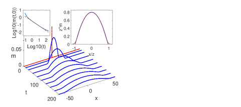
Figure 1: Time evolution of the density of agents. In this case $T=200$, $g=-2$, $\sigma=0.5$ and $\mu=1$. The initial distribution is a Gaussian of variance $0.1$, and the terminal cost is flat $c_{T}(x)=0$. The left inset shows the evolution of $m(t,0)=3/4z(t)$ with time (full line) compared to the $t^{2/3}$ scaling behavior (dashed). On the left inset are ploted an inverted parabola, and the density $m(x,t)$ rescaled by $z(t)$ for three different times.

Another necessary condition for this behavior to appear is the smallness of the healing length $\nu={\mu\sigma^{2}}/{|g|}$ with respect to other lengthscales, but it will be eventually fulfilled once the density distribution gets sufficiently extended (and at all times thereafter), possibly inducing a time shift in (6).

What those numerical results tell us is that in this configuration, the notion of ergodic state has been replaced by the next best thing, namely a universal scaling solution. The goal of this paper is to understand this puzzling result and in particular the $\frac{2}{3}$ scaling exponent.

We now introduce the few formal transformations which allow to show that this result is rather natural and intuitive, once the problem is cast in its proper language. In turn, we will also gain a better understanding of this regime

Hydrodynamic representation

The main idea underlying these transformations comes from the deep link between Mean Field Games and the nonlinear Schrödinger equation, discussed at lengths in Ullmo et al. (2019), which allows for the use of several techniques developed to study Bose-Einstein condensates. One of these techniques, the Madelung substitution, is particularly well suited to deal with the small $\nu$ regime Pethick and Smith (2008). It consists in defining a velocity field $v(t,x)$

$$v(x,t)=-\frac{\nabla u}{\mu}-\frac{\sigma^{2}\nabla m}{2m}\;,$$ (7)

which drives the evolution of the density $m$ as a simple transport/continuity equation

$$\partial_{t}m+\nabla(mv)=0\;.$$ (8)

The evolution for the velocity field $v$ derives from the HJB equation (4)

$$\partial_{t}v+\nabla\left[\frac{\sigma^{4}}{2\sqrt{m}}\Delta\sqrt{m}+\frac{v^{2}}{2}+\frac{g}{\mu}m\right]=0\;,$$ (9)

and involves a $O(\sigma^{4})$ term. As in the context of cold atoms, this term can be neglected as long as the characteristic length of the system is large in front of the healing length $\nu={\mu\sigma^{2}}/{|g|}$ Pethick and Smith (2008), leading to what is referred to as the Thomas Fermi approximation. This weak noise limit is also one of the requirements for the appearance of the parabolic behavior described in Figure 1. In this approximation the equation read

$$\left\{\begin{aligned} &\partial_{t}m+\nabla(mv)=0\\ &\partial_{t}v+\nabla\left[\frac{v^{2}}{2}+\frac{g}{\mu}m\right]=0\\ \end{aligned}\right.\;.$$ (10)

These equations are formally very close to those studied for instance in the field of cold atoms Dalfovo et al. (1999), the main differences being the (negative) sign of $g$, which makes the system elliptic rather than hyperbolic, and the nature of the boundary conditions. Within this approximation, it can easily be verified that the ansatz Eq. (5) with

$$z(t)=3\left(\frac{|g|}{4\mu}\right)^{1/3}\,t^{2/3}\;,$$ (11)

is a particular solution of the Thomas-Fermi-like equations Eq. (10). The real mystery is therefore not that such a solution does exist, but to understand why it is universal in the large optimization time limit.

Riemann invariant and hodograph transform

To answer this question, we shall turn to an approach developed in the context of non-linear waves Kamchatnov (2000), which relies on the notions of Riemann invariants and hodograph transform. Riemann’s method can be considered an extension of the method of characteristics. It amounts to finding curves (characteristics) on which some quantities (Riemann invariants) are conserved. Here, one can show that there exists a pair of Riemann invariants, $(\lambda_{+}(x,t),\lambda_{-}(x,t))$, namely $\lambda_{\pm}=v\pm 2i\sqrt{{|g|m}/{\mu}}$, so that (10) reads

$$\left\{\begin{aligned} &\partial_{t}\lambda_{+}+\left(\frac{3}{4}\lambda_{+}+\frac{1}{4}\lambda_{-}\right)\partial_{x}\lambda_{+}=0\\ &\partial_{t}\lambda_{-}+\left(\frac{1}{4}\lambda_{+}+\frac{3}{4}\lambda_{-}\right)\partial_{x}\lambda_{-}=0\end{aligned}\right.\;.$$ (12)

Though characteristics do not exist in this context (they are curves in the complex plane $\mathbb{C}^{2}$), this change of variables still allows us to linearize these equations using an hodograph transformation Kamchatnov (2000). Taking the pair $(\lambda_{+},\lambda_{-})$ as independant variables, we express $x$ and $t$ as functions of them, so that the system (12) transforms into a linear one:

$$\left\{\begin{aligned} &\partial_{\lambda_{-}}x-\beta_{+}\partial_{\lambda_{-}}t=0\\ &\partial_{\lambda_{+}}x-\beta_{-}\partial_{\lambda_{+}}t=0\end{aligned}\right.\;,$$ (13)

where $\beta_{\pm}=\left(\frac{3}{4}\lambda_{\pm}+\frac{1}{4}\lambda_{\mp}\right)$. This system can be readily integrated once as

$$\left\{\begin{aligned} &x-\beta_{+}t=\omega_{+}\\ &x-\beta_{-}t=\omega_{-}\end{aligned}\right.\;,$$ (14)

with $\omega_{\pm}$ solution of

$$\partial_{\lambda_{\pm}}\omega_{\mp}=-(\partial_{\lambda_{\pm}}\beta_{\mp})t=-\frac{1}{4}t\;.$$ (15)

Thus the functions $\omega_{\pm}$ can be expressed as derivatives of a potential $\omega_{\pm}=\partial_{\lambda_{\pm}}\chi$, where $\chi(\lambda_{+},\lambda_{-})$ is solution of an Euler-Poisson-Darboux equation:

$$\partial_{\lambda_{+}\lambda_{-}}\chi-\frac{1}{2(\lambda_{+}-\lambda_{-})}(\partial_{\lambda_{+}}\chi-\partial_{\lambda_{-}}\chi)=0\;.$$ (16)

The main difference with the traditional treatment of NLS that we have closely followed until now is that here the Riemann invariants $(\lambda_{+},\lambda_{-})$ are complex conjugates. In terms of its real and imaginary parts, $\xi=\frac{1}{2}(\lambda_{+}+\lambda_{-})=v$ and $\eta=\frac{1}{2i}(\lambda_{+}-\lambda_{-})=\;2\sqrt{{|g|m}/{\mu}}$, equation (16) becomes

$$\partial_{\xi\xi}\chi+\partial_{\eta\eta}\chi+\frac{1}{\eta}\partial_{\eta}\chi=0\;,$$ (17)

which is the Laplace equation in cylindrical coordinates (with no angular dependence) with $\eta$ and $\xi$ as radial and axial coordinates, respectively. Equations (14) now read

$$\left\{\begin{aligned} &\eta t=-E_{\eta}\\ &2(x-\xi t)=-E_{\xi}\end{aligned}\right.\;,$$ (18)

with $E_{\eta}$ and $E_{\xi}$ the radial and axial components of the electric field, ${\bf E}=-\nabla\chi$. Note that even if (17) is originally a two-dimensional problem, a clear connection with electrostatics emerges when considering it a three dimensional one with axial symmetry.

Potential representation

Through the hodograph transform we have shown that for any potential $\chi$, solution of the Laplace equation (17), there is a solution to the Thomas Fermi equation (10) provided that the relations (18) between $x$, $t$ and the electric field $\bf E$ hold. The linear Laplace equation (and the related electrostatic problem) is clearly significantly simpler than the original non-linear hydrodynamic equations. The price to pay for that simplification is that taking into account the boundary conditions becomes highly non trivial since the locus of the curves $t(\xi,\eta)=0$ or $t(\xi,\eta)=T$ on which these conditions are expressed actually depend on the particular potential $\chi(\xi,\eta)$ considered.

Since the dynamics we are interested in is related to the spreading of the density of agents, the time evolution is associated with a contraction towards the origin in the plane $(\xi,\eta)$ and the equal time curves, $t(\xi,\eta)=\text{const}$, are nested together, larger times closer to the origin. If we consider $\chi$ as generated by a distribution of charge $\rho(\xi,\eta)$, Eq. (17) implies that there is no charges between the curves $t(\xi,\eta)=0$ and $t(\xi,\eta)=T$ but $\rho(\xi,\eta)$ can be non-zero either near the origin (inside the curve $t(\xi,\eta)=T$) or at large distance (outside the curve $t(\xi,\eta)=0$). If the optimization time is long enough we can assume that there exists a large time inteval $[\tilde{t}_{\rm min},\tilde{t}_{\rm max}]$, $0\ll\tilde{t}_{\rm min}$, $\tilde{t}_{\rm max}\ll T$, so that at any time $t\in[\tilde{t}_{\rm min},\tilde{t}_{\rm max}]$, the details of the distibutions of charges both near the origin and outside the domain (using axial symmetry) can be essentially neglected, keeping only the most slowly decaying contribution. In that case a good approximation of $\chi$ is the potential created by a point charge $Q_{0}$ located at the origin

$$\chi(\eta,\xi)\approx\frac{Q_{0}}{\sqrt{\eta^{2}+\xi^{2}}}\;,$$ (19)

with a relation between $Q_{0}$ and the boundary conditions of the problem yet to be determined.

The main result of this paper is that the approximation of the charge distribution by a monopole centered at the origin is precisely the observed universal behavior expressed by Eqs. (5)-(6), and in particular the conditions under which this approximation is valid provide the regime of validity of the scaling form Eqs. (5)-(6). Indeed, inserting Eq. (19) into Eq. (18) and inverting the relation between $(\xi\!=\!v,\eta\!=\!\sqrt{|g|m/\mu})$ and $(x,t)$ readily gives

$$m(t,x) = \frac{\mu}{9|g|t^{2}}\left(\frac{9}{4}|Q_{0}|^{2/3}\,t^{4/3}-x^{2}\right)\;,$$ (20)

$$v(t,x) = \frac{2}{3}\;\frac{x}{t}\;.$$ (21)

Equation (20) identifies to (5) with $z(t)$ given by Eq. (11). In addition, normalization of $m(x,t)$ would require that the value of the charge is fixed, $Q_{0}=-2|g|/\mu$. We have now to show that this is actually the case independently of the boundary condition to prove that Eq. (20) is indeed the numerically observed scaling form Eqs. (5)-(6).

For this purpose, we simply apply Gauss’s law

$$Q_{0}=\frac{1}{4\pi}\int_{S_{\tilde{t}}}(\vec{E}\cdot\vec{n})dS\;$$ (22)

on a surface ${S_{\tilde{t}}}$ on which time is constant, $t(\eta,\xi)=\tilde{t}$, for some $t\in[0,T]$. Using $x$ and the dumy angle $\theta$ as coordinates on this surface, the surface element$dS$ and normal vector $\vec{n}$ read, respectively $dS=\eta j(x,\tilde{t})d\theta dx$ and $\vec{n}=(n_{\xi},n_{\eta},n_{\theta})=j(x,\tilde{t})^{-1}\left(\partial_{x}\xi,-\partial_{x}\eta,0\right)$, with $j(x,\tilde{t})\equiv\sqrt{(\partial_{x}\xi)^{2}+(\partial_{x}\eta)^{2}}$. We get

$$Q_{0} =\frac{1}{4\pi}\int_{0}^{2\pi}\int_{\mathbb{R}}\eta\left[2(x-\xi\tilde{t})\partial_{x}\eta-\eta\tilde{t}\partial_{x}\xi\right]d\theta dx$$ (23)

$$=\frac{1}{2}\int_{\mathbb{R}}\left[-\tilde{t}\partial_{x}(\eta^{2}\xi)+2x\eta\partial_{x}\eta\right]dx\;.$$

In the absence of mass flow at infinity, the first, time dependent, term integrates to zero. This appears here as a consequence of the fact that for all $\tilde{t}\in[0,T]$, the total charge enclosed in $S_{\tilde{t}}$ is the same and $Q_{0}$ is by construction a constant of motion. Integrating by part the second term and recalling that $\eta=2\sqrt{{|g|m}/{\mu}}$, Eq.(23) yields $Q_{0}=\frac{2g}{\mu}\int_{\mathbb{R}}mdx$ , which, because of the normalization condition $\int_{\mathbb{R}}mdx=1$, is the required result.

To conclude, we have shown that, using the potential representation of the [one dimensional potential-free] Mean Field Game problem we consider, the remarkable, and a priori quite puzzling universal scaling form which shows up in numerical simulations can be derived in a very natural way by approximating the charge distribution creating the electrostatic potential $\chi$ to a simple monopole. The condition that the observation point is sufficiently far from both the charges near the origin and the one near infinity underlying this approximation is equivalent to considering times far from both $t=0$ and $t=T$, which is of course only possible in the limit of very long optimization time. Furthermore, the electrostatic picture would allow for a more precise quantification of the conditions of validity of the approximation, using estimates on boundary conditions. We have thus been allowed to extend in some sense the notion of ergodic state to a situation where a genuine ergodic state cannot exist.

At a more general level, the potential representation of our Mean Field Games underlies the integrability of the hydrodynamical equations (10). Beyond the simple monopolar approximation Eq. (19), we can construct a complete multipolar expansion for the potential $\chi$, and it can be seen that each “charge” in this expansion relates to a conserved quantity of the dynamics. The mapping between the boundary conditions and these charges being thus equivalent to the mapping between boundary conditions and constants of motion. These considerations emphasize the fact that the deep reason behind the scaling law characterizing the 1d potential free MFG that we consider in this paper is actually their integrable character. A more in depth discussion of this question will appear in a subsequent publication.

References

- Lasry and Lions (2006) J.-M. Lasry and P.-L. Lions, C. R. Acad. Sci. Paris, Ser. I 343, 619 (2006).
- Lachapelle et al. (2015) A. Lachapelle, J.-M. Lasry, C.-A. Lehalle, and P.-L. Lions, arXiv:1305.6323 (2015).
- Lasry and Lions (2007) J.-M. Lasry and P.-L. Lions, Japanese Journal of Mathematics 2, 229 (2007).
- Guéant et al. (2011) O. Guéant, J.-M. Lasry, and P.-L. Lions, “Mean field games and applications,” in Paris-Princeton Lectures on Mathematical Finance 2010 (Springer, Heidelberg, 2011) pp. 205–266.
- Achdou et al. (2014) Y. Achdou, F. J. Buera, J.-M. Lasry, L. P.-L., and B. Moll, Phil. Trans. R. Soc. A 372, 20130397 (2014).
- Mériauxi et al. (2012) F. Mériauxi, V. Varma, and S. Lasaulce, in 2012 Conference Record of the Forty Sixth Asilomar Conference on Signals, Systems and Computers (ASILOMAR) (2012) pp. 671–675.
- Kizilkale and Malhamé (2016) A. Kizilkale and R. Malhamé, in Control of Complex Systems, edited by K. G. Vamvoudakis and S. Jagannathan (Butterworth-Heinemann, 2016) pp. 559 – 584.
- Bertsekas (2017) D. Bertsekas, Dynamic Programming and Optimal Control (Athena Scientific, Nashua, 2017).
- Ullmo et al. (2019) D. Ullmo, I. Swiecicki, and T. Gobron, Physics Reports 799, 1 (2019).
- Cardaliaguet et al. (2013) P. Cardaliaguet, J.-M. Lasry, P.-L. Lions, and A. Porretta, SIAM J. Control Optim. 51, 3558 (2013), http://dx.doi.org/10.1137/120904184 .
- Pethick and Smith (2008) C. J. Pethick and H. Smith, Bose-Einstein Condensation in Dilute Gases, 2nd ed. (Cambridge University Press, 2008).
- Dalfovo et al. (1999) F. Dalfovo, S. Giorgini, L. P. Pitaevskii, and S. Stringari, Reviews of Modern Physics 71, 463 (1999).
- Kamchatnov (2000) A. Kamchatnov, Nonlinear Periodic Waves and Their Modulations: An Introductory Course (World Scientific, 2000).