Time2Vec: Learning a Vector Representation of Time

Abstract

Time is an important feature in many applications involving events that occur synchronously and/or asynchronously. To effectively consume time information, recent studies have focused on designing new architectures. In this paper, we take an orthogonal but complementary approach by providing a model-agnostic vector representation for time, called Time2Vec, that can be easily imported into many existing and future architectures and improve their performances. We show on a range of models and problems that replacing the notion of time with its Time2Vec representation improves the performance of the final model.

1 Introduction

In building machine learning models, “time” is often an important feature. Examples include predicting daily sales for a company based on the date (and other available features), predicting the time for a patient’s next health event based on their medical history, and predicting the song a person is interested in listening to based on their listening history. The input for problems involving time can be considered as a sequence where, rather than being identically and independently distributed (iid), there exists a dependence across time (and/or space) among the data points. The sequence can be either synchronous, i.e. sampled at regular intervals, or asynchronous, i.e. sampled at different points in time. In both cases, time may be an important feature. For predicting daily sales, for instance, it may be useful to know if it is a holiday or not. For predicting the time for a patient’s next encounter, it is important to know the (asynchronous) times of their previous visits.

Recurrent neural networks (RNNs) [23, 9] have achieved impressive results on a range of sequence modeling problems. Most RNN models do not treat time itself as a feature, typically assuming that inputs are synchronous. When time is known to be a relevant feature, it is often fed in as yet another input dimension [10, 14, 35]. In practice, RNNs often fail at effectively making use of time as a feature. To help the RNN make better use of time, several researchers design hand-crafted features of time that suit their specific problem and feed those features into the RNN [10, 3, 29]. Hand-crafting features, however, can be expensive and requires domain expertise about the problem.

Many recent studies aim at obviating the need for hand-crafting features by proposing general-purpose—as opposed to problem specific—architectures that better handle time [44, 61, 39, 24, 56, 34]. We follow an orthogonal but complementary approach to these recent studies by developing a general-purpose model-agnostic representation for time that can be potentially used in any architecture. In particular, we develop a learnable vector representation (or embedding) for time as a vector representation can be easily combined with many models or architectures. We call this vector representation Time2Vec. To validate the effectiveness of Time2Vec, we conduct experiments on several (synthesized and real-world) datasets and integrate it with several architectures. Our main result is to show that on a range of problems and architectures that consume time, using Time2Vec instead of the time itself offers a boost in performance.

2 Related Work

There is a long history of algorithms for predictive modeling in time series analysis. They include auto-regressive techniques [1] that predict future measurements in a sequence based on a window of past measurements. Since it is not always clear how long the window of past measurements should be, hidden Markov models [50], dynamic Bayesian networks [42], and dynamic conditional random fields [53] use hidden states as a finite memory that can remember information arbitrarily far in the past. These models can be seen as special cases of recurrent neural networks [23]. They typically assume that inputs are synchronous, i.e. arrive at regular time intervals, and that the underlying process is stationary with respect to time. It is possible to aggregate asynchronous events into time-bins and to use synchronous models over the bins [36, 2]. Asynchronous events can also be directly modeled with point processes (e.g., Poisson, Cox, and Hawkes point processes) [12, 31, 59, 34, 60] and continuous time normalizing flows [8]. Alternatively, one can also interpolate or make predictions at arbitrary time stamps with Gaussian processes [51] or support vector regression [13].

Our goal is not to propose a new model for time series analysis, but instead to propose a representation of time in the form of a vector embedding that can be used by many models. Vector embedding has been previously successfully used for other domains such as text [40, 48], (knowledge) graphs [22, 46, 25], and positions [57, 17]. Our approach is related to time decomposition techniques that encode a temporal signal into a set of frequencies [11]. However, instead of using a fixed set of frequencies as in Fourier transforms [5], we allow the frequencies to be learned. We take inspiration from the neural decomposition of Godfrey and Gashler [20] (and similarly [16]). For time-series analysis, Godfrey and Gashler [20] decompose a 1D signal of time into several sine functions and a linear function to extrapolate (or interpolate) the given signal. We follow a similar intuition but instead of decomposing a 1D signal of time into its components, we transform the time itself and feed its transformation into the model that is to consume the time information. Our approach corresponds to the technique of Godfrey and Gashler [20] when applied to regression tasks in 1D signals, but it is more general since we learn a representation that can be shared across many signals and can be fed to many models for tasks beyond regression.

While there is a body of literature on designing neural networks with sine activations [30, 52, 58, 41, 37], our work uses sine only for transforming time; the rest of the network uses other activations. There is also a set of techniques that consider time as yet another feature and concatenate time (or some hand designed features of time such as log and/or inverse of delta time) with the input [10, 33, 14, 3, 29, 55, 28, 38]. Kazemi et al. [26] survey several such approaches for dynamic (knowledge) graphs. These models can directly benefit from our proposed vector embedding, Time2Vec, by concatenating Time2Vec with the input instead of their time features. Other works [44, 61, 39, 24, 56, 34] propose new neural architectures that take into account time (or some features of time). As a proof of concept, we show how Time2Vec can be used in one of these architectures to better exploit temporal information; it can be potentially used in other architectures as well.

3 Background & Notation

We use lower-case letters to denote scalars, bold lower-case letters to denote vectors, and bold upper-case letters to denote matrices. We represent the $i^{th}$ element of the vector $\boldsymbol{r}$ as $\boldsymbol{r}[i]$. For two vectors $\boldsymbol{r}$ and $\boldsymbol{s}$, we use $[\boldsymbol{r};\boldsymbol{s}]$ to represent their concatenation and $\boldsymbol{r}\odot\boldsymbol{s}$ to represent element-wise (Hadamard) multiplication of the two vectors. Throughout the paper, we use $\tau$ to represent a scalar notion of time (e.g., absolute time, time from start, time from the last event, etc.) and $\boldsymbol{\tau}$ to represent a vector of time features.

Long Short Term Memory (LSTM) [23] is considered one of the most successful RNN architectures for sequence modeling. A formulation of the original LSTM model and a variant of it based on peepholes [18] is presented in Appendix C. When time is a relevant feature, the easiest way to handle time is to consider it as just another feature (or extract some engineered features from it), concatenate the time features with the input, and use the standard LSTM model (or some other sequence model) [10, 14, 35]. In this paper, we call this model LSTM+T. Another way of handling time is by changing the formulation of the standard LSTM. Zhu et al. [61] developed one such formulation, named TimeLSTM, by adding time gates to the architecture of the LSTM with peepholes. They proposed three architectures namely TLSTM1, TLSTM2, TLSTM3. A description of TLSTM1 and TLSTM3 can be found in Appendix C (we skipped TLSTM2 as it is quite similar to TLSTM3).

4 Time2Vec

In designing a representation for time, we identify three important properties: 1- capturing both periodic and non-periodic patterns, 2- being invariant to time rescaling, and 3- being simple enough so it can be combined with many models. In what follows, we provide more detail on these properties.

Periodicity: In many scenarios, some events occur periodically. The amount of sales of a store, for instance, may be higher on weekends or holidays. Weather condition usually follows a periodic pattern over different seasons [16]. Some notes in a piano piece usually repeat periodically [24]. Some other events may be non-periodic but only happen after a point in time and/or become more probable as time proceeds. For instance, some diseases are more likely for older ages. Such periodic and non-periodic patterns distinguish time from other features calling for better treatment and a better representation of time. In particular, it is important to use a representation that enables capturing periodic and non-periodic patterns.

Invariance to Time Rescaling: Since time can be measured in different scales (e.g., days, hours, seconds, etc.), another important property of a representation for time is invariance to time rescaling (see, e.g., [54]). A class $\mathcal{C}$ of models is invariant to time rescaling if for any model $\mathcal{M}_{1}\in\mathcal{C}$ and any scalar $\alpha>0$, there exists a model $\mathcal{M}_{2}\in\mathcal{C}$ that behaves on $\alpha\tau$ ($\tau$ scaled by $\alpha$) in the same way $\mathcal{M}_{1}$ behaves on original $\tau$s.

Simplicity: A representation for time should be easily consumable by different models and architectures. A matrix representation, for instance, may be difficult to consume as it cannot be easily appended with the other inputs.

Time2Vec: We propose Time2Vec, a representation for time which has the three identified properties. For a given scalar notion of time $\tau$, Time2Vec of $\tau$, denoted as $\text{{t2v}}(\tau)$, is a vector of size $k+1$ defined as follows:

$$\text{{t2v}}(\tau)[i]=\begin{cases}\omega_{i}\tau+\varphi_{i},&\text{if~{}~{}$i=0$}.\\ \mathcal{F}{(\omega_{i}\tau+\varphi_{i})},&\text{if~{}~{}$1\leq i\leq k$}.\end{cases}$$ (1)

where $\text{{t2v}}(\tau)[i]$ is the $i^{th}$ element of $\text{{t2v}}(\tau)$, $\mathcal{F}$ is a periodic activation function, and $\omega_{i}$s and $\varphi_{i}$s are learnable parameters. Given the prevalence of vector representations for different tasks, a vector representation for time makes it easily consumable by different architectures. We chose $\mathcal{F}$ to be the sine function in our experiments but we do experiments with other periodic activations as well. When $\mathcal{F}=\sin$, for $1\leq i\leq k$, $\omega_{i}$ and $\varphi_{i}$ are the frequency and the phase-shift of the sine function.

The period of $\sin{(\omega_{i}\tau+\varphi_{i})}$ is $\frac{2\pi}{\omega_{i}}$, i.e. it has the same value for $\tau$ and $\tau+\frac{2\pi}{\omega_{i}}$. Therefore, a sine function helps capture periodic behaviors without the need for feature engineering. For instance, a sine function $\sin{(\omega\tau+\varphi)}$ with $\omega=\frac{2\pi}{7}$ repeats every $7$ days (assuming $\tau$ indicates days) and can be potentially used to model weekly patterns. Furthermore, unlike other basis functions which may show strange behaviors for extrapolation (see, e.g., [49]), sine functions are expected to work well for extrapolating to future and out of sample data [57]. The linear term represents the progression of time and can be used for capturing non-periodic patterns in the input that depend on time. Proposition 1 establishes the invariance of Time2Vec to time rescaling. The proof is in Appendix D.

Proposition 1.

Time2Vec is invariant to time rescaling.

The use of sine functions is inspired in part by Vaswani et al. [57]’s positional encoding. Consider a sequence of items (e.g., a sequence of words) $\{I_{1},I_{2},\dots,I_{N}\}$ and a vector representation $\boldsymbol{v}_{I_{j}}\in\mathbb{R}^{d}$ for the $j^{th}$ item $I_{j}$ in the sequence. Vaswani et al. [57] added $\sin{(j/10000^{k/d})}$ to $\boldsymbol{v}_{I_{j}}[k]$ if $k$ is even and $\sin{(j/10000^{k/d}+\pi/2)}$ if $k$ is odd so that the resulting vector includes information about the position of the item in the sequence. These sine functions are called the positional encoding. Intuitively, positions can be considered as the times and the items can be considered as the events happening at that time. Thus, Time2Vec can be considered as representing continuous time, instead of discrete positions, using sine functions. The sine functions in Time2Vec also enable capturing periodic behaviors which is not a goal in positional encoding. We feed Time2Vec as an input to the model (or to some gate in the model) instead of adding it to other vector representations. Unlike positional encoding, we show in our experiments that learning the frequencies and phase-shifts of sine functions in Time2Vec result in better performance compared to fixing them.

5 Experiments & Results

We design experiments to answer the following questions: Q1: is Time2Vec a good representation for time?, Q2: can Time2Vec be used in other architectures and improve their performance?, Q3: what do the sine functions learn?, Q4: can we obtain similar results using non-periodic activation functions for Eq. (23) instead of periodic ones?, and Q5: is there value in learning the sine frequencies or can they be fixed (e.g., to equally-spaced values as in Fourier sine series or exponentially-decaying values as in Vaswani et al. [57]’s positional encoding)? We use the following datasets:

1) Synthesized data: We create a toy dataset to use for explanatory experiments. The inputs in this dataset are the integers between $1$ and $365$. Input integers that are multiples of $7$ belong to class one and the other integers belong to class two. The first 75% is used for training and the last 25% for testing. This dataset is inspired by the periodic patterns (e.g., weekly or monthly) that often exist in daily-collected data; the input integers can be considered as the days.

2) Event-MNIST: Sequential (event-based) MNIST is a common benchmark in sequence modeling literature (see, e.g., [4, 6, 15]). We create a sequential event-based version of MNIST by flattening the images and recording the position of the pixels whose intensities are larger than a threshold ($0.9$ in our experiment). Following this transformation, each image will be represented as an array of increasing numbers such as $[t_{1},t_{2},t_{3},\dots,t_{m}]$. We consider these values as the event times and use them to classify the images. As in other sequence modeling works, our aim in building this dataset is not to beat the state-of-the-art on the MNIST dataset; our aim is to provide a dataset where the only input is time and different representations for time can be compared when extraneous variables (confounders) are eliminated as much as possible.

3) N_TIDIGITS18 [2]: The dataset includes audio spikes of the TIDIGITS spoken digit dataset [32] recorded by the binaural 64-channel silicon cochlea sensor. Each sample is a sequence of $(t,c)$ tuples where $t$ represents time and $c$ denotes the index of active frequency channel at time $t$. The labels are sequences of 1 to 7 connected digits with a vocabulary consisting of 11 digits (i.e. “zero” to “nine” plus “oh”) and the goal is to classify the spoken digit based on the given sequence of active channels. We use the reduced version of the dataset where only the single digit samples are used for training and testing. The reduced dataset has a total of 2,464 training and 2,486 test samples.

4) Stack Overflow (SOF): This dataset contains sequences of badges obtained by stack overflow users and the timestamps at which the badges were obtained. We used the subset released by Du et al. [14] containing $\sim 6K$ users, $22$ event types (badges), and $\sim 480K$ events. Given a sequence $[(b_{1}^{u},t_{1}^{u}),(b_{2}^{u},t_{2}^{u}),...,(b_{n}^{u},t_{n}^{u})]$ for each user $u$ where $b_{i}^{u}$ is the badge id and $t_{i}^{u}$ is the timestamp when $u$ received this badge id, the task is to predict the badge the user will obtain at time $t_{k+1}^{u}$.

5) Last.FM: This dataset contains a history of listening habits for Last.FM users [7]. We used the code released by Zhu et al. [61] to pre-process the data. The dataset contains $\sim 1K$ users, 5000 event types (songs), and $\sim 819K$ events. The prediction problem is similar to the SOF dataset but with dynamic updating (see, [61] for details).

6) CiteULike: This dataset contains data about what and when a user posted on citeulike website. The original dataset has about 8000 samples. Similar to Last.FM, we used the pre-processing used by Zhu et al. [61] to select $\sim 1.6K$ sequences with 5000 event types (papers) and $\sim 36K$ events. The task for this dataset is similar to that for Last.FM.

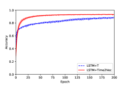
(a) Event-MNIST

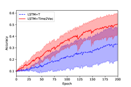
(b) Raw N_TIDIGITS18

(c) Stack Overflow

(d) Last.FM

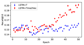
(e) CiteULike

Figure 1: Comparing LSTM+T and LSTM+Time2Vec on several datasets.

Measures: For classification tasks, we report accuracy corresponding to the percentage of correctly classified examples. For recommendation tasks, we report Recall@q and MRR@q. Following Zhu et al. [61], to generate a recommendation list, we sample $k-1$ random items and add the correct item to the sampled list resulting in a list of $k$ items. Then our model ranks these $k$ items. Looking only at the top ten recommendations, Recall@q corresponds to the percentage of recommendation lists where the correct item is in the top $q$; MRR@q (reported in Appendix B) corresponds to the mean of the inverses of the rankings of the correct items where the inverse rank is considered $0$ if the item does not appear in top $q$ recommendations. For Last.FM and CiteULike, following Zhu et al. [61] we report Recall@10 and MRR@10. For SOF, we report Recall@3 and MRR as there are only $22$ event types and Recall@10 and MRR@10 are not informative enough. The detail of the implementations is presented in Appendix A.

5.1 On the effectiveness of Time2Vec

Fig. 1 represents the obtained results of comparing LSTM+Time2Vec with LSTM+T on several datasets with different properties and statistics. It can be observed that on all datasets, replacing time with Time2Vec improves the performance in most cases and never deteriorates it; in many cases, LSTM+Time2Vec performs consistently better than LSTM+T. Anumula et al. [2] mention that LSTM+T fails on N_TIDIGITS18 as the dataset contains very long sequences. By feeding better features to the LSTM rather than relying on the LSTM to extract them, Time2Vec helps better optimize the LSTM and offers higher accuracy (and lower variance) compared to LSTM+T. Besides N_TIDIGITS18, SOF also contains somewhat long sequences and long time horizons. The results on these two datasets indicate that Time2Vec can be effective for datasets with long sequences and time horizons. From the results obtained in this subsection, it can be observed that Time2Vec is indeed an effective representation of time thus answering Q1 positively.

To verify if Time2Vec can be integrated with other architectures and improve their performance, we integrate it with TLSTM1 and TLSTM3, two recent and powerful models for handling asynchronous events. To use Time2Vec in these two architectures, we replaced their notion $\tau$ of time with $\text{{t2v}}(\tau)$ and replaced the vectors getting multiplied to $\tau$ with matrices accordingly. The updated formulations are presented in Appendix C. The obtained results in Fig. 2 for TLSTM1 and TLSTM3 on Last.FM and CiteULike demonstrates that replacing time with Time2Vec for both TLSTM1 and TLSTM3 improves the performance thus answering Q2 affirmatively positively.

5.2 What does Time2Vec learn?

To answer Q3, we trained a model on our synthesized dataset where the input integer (day) is used as the time for Time2Vec and a fully connected layer is used on top of the Time2Vec to predict the class. That is, the probability of one of the classes is a sigmoid of a weighted sum of the Time2Vec elements. Fig. 3 (a) shows a the learned function for the days in the test set where the weights, frequencies and phase-shifts are learned from the data. The red dots on the figure represent multiples of $7$. It can be observed that Time2Vec successfully learns the correct period and oscillates every $7$ days. The phase-shifts have been learned in a way that all multiples of $7$ are placed on the positive peaks of the signal to facilitate separating them from the other days. Looking at the learned frequency and phase-shift for the sine functions across several runs, we observed that in many runs one of the main sine functions has a frequency around $0.898\approx\frac{2\pi}{7}$ and a phase-shift around $1.56\approx\frac{\pi}{2}$, thus learning to oscillate every $7$ days and shifting by $\frac{\pi}{2}$ to make sure multiples of $7$ end up at the peaks of the signal. Fig. 4 shows the initial and learned sine frequencies for one run. It can be viewed that at the beginning, the weights and frequencies are random numbers. But after training, only the desired frequency ($\frac{2\pi}{7}$) has a high weight (and the $0$ frequency which gets subsumed into the bias). The model perfectly classifies the examples in the test set which represents the sine functions in Time2Vec can be used effectively for extrapolation and out of sample times assuming that the test set follows similar periodic patterns as the train set. We added some noise to our labels by flipping $5\%$ of the labels selected at random and observed a similar performance in most runs.

To test invariance to time rescaling, we multiplied the inputs by $2$ and observed that in many runs, the frequency of one of the main sine functions was around $0.448\approx\frac{2\pi}{2*7}$ thus oscillating every $14$ days. An example of a combination of signals learned to oscillate every $14$ days is in Fig. 3 (b).

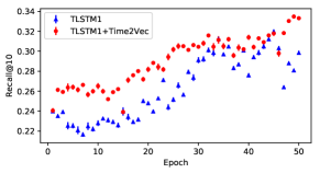
(a) TLSTM1, Last.FM

(b) TLSTM1, CiteULike

(c) TLSTM3, Last.FM

(d) TLSTM3, CiteULike

Figure 2: Comparing TLSTM1 and TLSTM3 on Last.FM and CiteULike in terms of Recall@10 with and without Time2Vec.

5.3 Other activation functions

To answer Q4, we repeated the experiment on Event-MNIST in Section 5.1 when using activation functions other than sine including non-periodic functions such as Sigmoid, Tanh, and rectified linear units (ReLU) [43], and periodic activation functions such as mod and triangle. We fixed the length of the Time2Vec to $64+1$, i.e. $64$ units with a non-linear transformation and $1$ unit with a linear transformation. From the results shown in Fig. 5(a), it can be observed that the periodic activation functions (sine, mod, and triangle) outperform the non-periodic ones. Other than not being able to capture periodic behaviors, we believe one of the main reasons why these non-periodic activation functions do not perform well is because as time goes forward and becomes larger, Sigmoid and Tanh saturate and ReLU either goes to zero or explodes.

Among periodic activation functions, sine outperforms the other two. The comparative effectiveness of the sine functions in processing time-series data with periodic behavior is unsurprising; An analogy can be drawn to the concept of Fourier series, which is a well established method of representing periodic signals. From this perspective, we can interpret the output of Time2Vec as representing periodic features which force the model to learn periodic attributes that are relevant to the task under consideration. This can be shown mathematically by expanding out the output of the first layer of any sequence model under consideration. Generally, the output of the first layer, after the Time2Vec transformation and before applying a non-linear activation, has the following form $\boldsymbol{a}=\boldsymbol{\Theta}\text{{t2v}}{\left(\tau\right)}$, where $\boldsymbol{\Theta}$ is the first layer weights matrix having components $\left[\boldsymbol{\Theta}\right]_{i,j}=\theta_{i,j}$. It follows directly from Eq. (23) that $\boldsymbol{a}(\tau,k)[i]=\theta_{i,0}(\omega_{0}\tau+\varphi_{0})+\sum_{j=1}^{k}\theta_{i,j}\sin\left(\omega_{i}\tau+\varphi_{i}\right)$, where $k-1$ is the number of sine functions used in the Time2Vec transformation. Hence, the first layer has transformed time $\tau$ into $n$ (output dimension of first layer) distinct features. The linear term $\theta_{i,0}(\omega_{0}\tau+\varphi_{0})$ can model non-periodic components and helps with extrapolation [20]. The second term (the sum of the weighted sine functions) can be used to model the periodic behavior of the $\boldsymbol{a}[i]$ features. Each component $\boldsymbol{a}[i]$ of the attribute vector will latch on to different relevant signals with different underlying frequencies such that each component $\boldsymbol{a}[i]$ can be viewed as representing distinct temporal attributes (having both a periodic and non-periodic part). The function can model a real Fourier signal when the frequencies $\omega_{i}$ of the sine functions are integer multiples of a base (first harmonic) frequency (and $\omega_{k+1}=0$). However, we show in Section 5.4 that learning the frequencies results in better generalization.

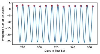
(a) A weighted sum of the sinusoids in Time2Vec oscillating every $7$ days.

(b) A weighted sum of the sinusoids in Time2Vec oscillating every $14$ days.

Figure 3: The models learned for our synthesized dataset explained in Subsection 5.2 before the final activation. The red dots represent the points to be classified as $1$.

Figure 4: (a) Initial vs. (b) learned weights and frequencies for our synthesized dataset.

5.4 Fixed frequencies and phase-shifts

According to Fourier sine series, any function can be closely approximated using sine functions with equally-spaced frequencies. Vaswani et al. [57] mention that learning sine frequencies and phase-shifts for their positional encoding gives the same performance as fixing frequencies to exponentially-decaying values and phase-shifts to $0$ and $\frac{\pi}{2}$. This raises the question of whether learning the sine frequencies and phase-shifts of Time2Vec from data offer any advantage compared to fixing them. To answer this question, we compare three models on Event-MNIST when using Time2Vec of length $16+1$: 1- fixing $\text{{t2v}}(\tau)[n]$ to $\sin{(\frac{2\pi n}{16})}$ for $n\leq 16$, 2- fixing the frequencies and phase shifts according to Vaswani et al. [57]’s positional encoding, and 3- learning the frequencies and phase-shifts from the data. Fig. 5(b) represents our obtained results. The obtained results in Fig. 5(b) show that learning the frequencies and phase-shifts rather than fixing them helps improve the performance of the model and provides the answer to Q5.

5.5 The use of periodicity in sine functions

It has been argued that when sine is used as the activation function, only a monotonically increasing (or decreasing) part of it is used and the periodic part is ignored [19]. When we use Time2Vec, however, the periodicity of the sine functions are also being used and seem to be key to the effectiveness of the Time2Vec representation. Fig. 5(c) shows some statistics on the frequencies learned for Event-MNIST where we count the number of learned frequencies that fall within intervals of lengths $0.1$ centered at $[0.05,0.15,\dots,0.95]$ (all learned frequencies are between $0$ and $1$). The figure contains two peaks at $0.35$ and $0.85$. Since the input to the sine functions for this problem can have a maximum value of $784$ (number of pixels in an image), sine functions with frequencies around $0.35$ and $0.85$ finish (almost) $44$ and $106$ full periods. The smallest learned frequency is $0.029$ which finishes (almost) $3.6$ full periods. These values indicate that the model is indeed using the periodicity of the sine functions, not just a monotonically increasing (or decreasing) part of them.

5.6 Why capture non-periodic patterns?

We argued in Section 4 that a representation of time needs to capture both periodic and non-periodic patterns. The sine functions in Time2Vec can be used to capture periodic patterns and the linear term can be used to capture non-periodic ones. In Section 5.1, we showed that capturing both periodic and non-periodic patterns (i.e. LSTM+Time2Vec) gives better performance than only capturing non-periodic patterns (i.e. LSTM+T). A question that remains to be answered is whether capturing both periodic and non-periodic patterns gives better performance than only capturing periodic patterns. To answer this question, we first repeated the experiment for Event-MNIST when the linear term is removed from Time2Vec but observed that the results were not affected substantially. This means capturing periodic patterns may suffice for Event-MNIST. Then we conducted a similar experiment for TLSTM3 on CiteULike and obtained the results in Fig. 5(d). From these results, we can see that capturing both periodic and non-periodic patterns makes a model perform better than only capturing periodic patterns. This experiment can also be viewed as an ablation study indicating why a linear term is required in Time2Vec.

(a)

(b)

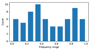
(c)

(d)

Figure 5: An ablation study of several components in Time2Vec. (a) Comparing different activation functions for Time2Vec on Event-MNIST. Sigmoid and Tanh almost overlap. (b) Comparing frequencies fixed to equally-spaced values, frequencies fixed according to positional encoding [57], and learned frequencies on Event-MNIST. (c) A histogram of the frequencies learned in Time2Vec for Event-MNIST. The x-axis represents frequency intervals and the y-axis represents the number of frequencies in that interval. (d) The performance of TLSTM3+Time2Vec on CiteULike in terms of Recall@10 with and without the linear term.

6 Conclusion & Future Work

In a variety of tasks for synchronous or asynchronous event predictions, time is an important feature with specific characteristics (progression, periodicity, scale, etc.). In this work, we presented an approach that automatically learns features of time that represent these characteristics. In particular, we developed Time2Vec, a vector representation for time, using sine and linear activations and showed the effectiveness of this representation across several datasets and several tasks. In the majority of our experiments, Time2Vec improved our results, while the remaining results were not hindered by its application. While sine functions have been argued to complicate the optimization [30, 19], we did not experience such a complication except for the experiment in Subsection 5.2 when using only a few sine functions. We hypothesize that the main reasons include combining sine functions with a powerful model (e.g., LSTM) and using many sine functions which reduces the distance to the goal (see, e.g., [45]). We leave a deeper theoretical analysis of this hypothesis and the development of better optimizers as future work.

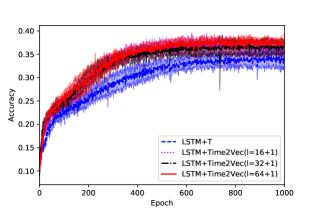
Figure 6: Comparing LSTM+T and LSTM+Time2Vec on Event-MNIST.

(a) Event-MNIST

(b) Raw N_TIDIGITS18

Figure 7: Comparing LSTM+T and LSTM+Time2Vec on Event-MNIST and raw N_TIDIGITS18.

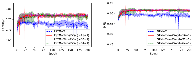
Figure 8: Comparing LSTM+T and LSTM+Time2Vec on SOF.

Figure 9: Comparing LSTM+T and LSTM+Time2Vec on Last.FM.

Figure 10: Comparing LSTM+T and LSTM+Time2Vec on CiteULike.

Appendix A Implementation Detail

For the experiments on Event-MNIST, N_TIDIGITS18 and SOF, we implemented our model in PyTorch [47]. We used Adam optimizer [27] with a learning rate of $0.001$. For Event-MNIST and SOF, we fixed the hidden size of the LSTM to $128$. For N_TIDIGITS18, due to its smaller train set, we fixed the hidden size to $64$. We allowed each model $200$ epochs. We used a batch size of $512$ for Event-MNIST and $128$ for N_TIDIGITS18 and SOF. For the experiments on Last.FM and CiteULike, we used the code released by Zhu et al. [61] without any modifications, except replacing $\tau$ with $\text{{t2v}}(\tau)$. The only other thing we changed in their code was to change the SAMPLE_TIME variable from $3$ to $20$. SAMPLE_TIME controls the number of times we do sampling to compute Recall@10 and MRR@10. We experienced a high variation when sampling only $3$ times so we increased the number of times we sample to $20$ to make the results more robust. For both Last.FM and CiteULike, Adagrad optimizer is used with a learning rate of $0.01$, vocabulary size is $5000$, and the maximum length of the sequence is $200$. For Last.FM, the hidden size of the LSTM is $128$ and for CiteULike, it is $256$. For all except the synthesized dataset, we shifted the event times such that the first event of each sequence starts at time $0$.

For the fairness of the experiments, we made sure the competing models for all our experiments have an (almost) equal number of parameters. For instance, since adding Time2Vec as an input to the LSTM increases the number of model parameters compared to just adding time as a feature, we reduced the hidden size of the LSTM for this model to ensure the number of model parameters stays (almost) the same. For the experiments involving Time2Vec, unless stated otherwise, we tried vectors with $16$, $32$ and $64$ sine functions (and one linear term). We reported the vector length offering the best performance in the main text. The results for other vector lengths can be found in Appendix B. For the synthetic dataset, we use Adam optimizer with a learning rate of $0.001$ without any regularization. The length of the Time2Vec vector is $32$.

Appendix B More Results

We ran experiments on other versions of the N_TIDIGITS18 dataset as well. Following [2], we converted the raw event data to event-binned features by virtue of aggregating active channels through a period of time in which a pre-defined number of events occur. The outcome of binning is thus consecutive frames each with multiple but a fixed number of active channels. In our experiments, we used event-binning with 100 events per frame. For this variant of the dataset, we compared LSTM+T and LSTM+Time2Vec similar to the experiments in Section 5.1. The obtained results were on-par. Then, similar to Event-MNIST, we only fed as input the times at which events occurred (i.e. we removed the channels from the input). We allowed the models $1000$ epochs to make sure they converge. The obtained results are presented in Fig. 6. It can be viewed that Time2Vec provides an effective representation for time and LSTM+Time2Vec outperforms LSTM+T on this dataset.

Figure 11: TLSTM1’s performance on Last.FM with and without Time2Vec.

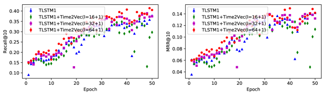
Figure 12: TLSTM1’s performance on CiteULike  with and without Time2Vec.

In the main text, for the experiments involving Time2Vec, we tested Time2Vec vectors with $16$, $32$ and $64$ sine functions and reported the best one for the clarity of the diagrams. Here, we show the results for all frequencies. Figures 7, 8, 9, and 10 compare LSTM+T and LSTM+Time2Vec for our datasets. Figures 11, and 12 compare TLSTM1 with TLSTM1+Time2Vec on Last.FM and CiteULike. Figures 13, and 14 compare TLSTM3 with TLSTM1+Time2Vec on Last.FM and CiteULike. In most cases, Time2Vec with 64 sine functions outperforms (or gives on-par results with) the cases with 32 or 16 sine functions. An exception is TLSTM3 where 16 sine functions works best. We believe that is because TLSTM3 has two time gates and adding, e.g., 64 temporal components (corresponding to the sine functions) to each gate makes it overfit to the temporal signals.

Appendix C LSTM Architectures

The original LSTM model can be neatly defined with the following equations:

$$\boldsymbol{i}_{j}=\sigma\left(\boldsymbol{W}_{i}\boldsymbol{x}_{j}+\boldsymbol{U}_{i}\boldsymbol{h}_{j-1}+\boldsymbol{b}_{i}\right)$$ (2)

$$\boldsymbol{f}_{j}=\sigma\left(\boldsymbol{W}_{f}\boldsymbol{x}_{j}+\boldsymbol{U}_{f}\boldsymbol{h}_{j-1}+\boldsymbol{b}_{f}\right)$$ (3)

$$\overline{\boldsymbol{c}}_{j}=Tanh\left(\boldsymbol{W}_{c}\boldsymbol{x}_{j}+\boldsymbol{U}_{c}\boldsymbol{h}_{j-1}+\boldsymbol{b}_{c}\right)$$ (4)

$$\boldsymbol{c}_{j}=\boldsymbol{f}_{t}\odot\boldsymbol{c}_{j-1}+\boldsymbol{i}_{j}\odot\overline{\boldsymbol{c_{j}}}$$ (5)

$$\boldsymbol{o}_{j}=\sigma\left(\boldsymbol{W}_{o}\boldsymbol{x}_{j}+\boldsymbol{U}_{o}\boldsymbol{h}_{j-1}+\boldsymbol{b}_{o}\right)$$ (6)

$$\boldsymbol{h}_{j}=\boldsymbol{o}_{j}\odot Tanh\left(\boldsymbol{c}_{j}\right)$$ (7)

Here $\boldsymbol{i}_{t}$, $\boldsymbol{f}_{t}$, and $\boldsymbol{o}_{t}$ represent the input, forget and output gates respectively, while $\boldsymbol{c}_{t}$ is the memory cell and $\boldsymbol{h}_{t}$ is the hidden state. $\sigma$ and $Tanh$ represent the Sigmoid and hyperbolic tangent activation functions respectively. We refer to $\boldsymbol{x}_{j}$ as the $j^{th}$ event.

Peepholes: Gers and Schmidhuber [18] introduced a variant of the LSTM architecture where the input, forget, and output gates peek into the memory cell. In this variant, $\boldsymbol{w}_{pi}\odot\boldsymbol{c}_{j-1}$, $\boldsymbol{w}_{pf}\odot\boldsymbol{c}_{j-1}$, and $\boldsymbol{w}_{po}\odot\boldsymbol{c}_{j}$ are added to the linear parts of Eq. (2), (3), and (6) respectively, where $\boldsymbol{w}_{pi}$, $\boldsymbol{w}_{pf}$, and $\boldsymbol{w}_{po}$ are learnable parameters.

Figure 13: TLSTM3’s performance on Last.FM  with and without Time2Vec.

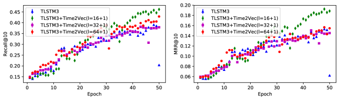
Figure 14: TLSTM3’s performance on CiteULike  with and without Time2Vec.

LSTM+T: Let $\boldsymbol{\tau}_{j}$ represent the time features for the $j^{th}$ event in the input and let $\boldsymbol{x}^{\prime}_{j}=[\boldsymbol{x}_{j};\boldsymbol{\tau}_{j}]$. Then LSTM+T uses the exact same equations as the standard LSTM (denoted above) except that $\boldsymbol{x}_{j}$ is replaced with $\boldsymbol{x}^{\prime}_{j}$.

TimeLSTM: We explain TLSTM1 and TLSTM3 which have been used in our experiments. For clarity of writing, we do not include the peephole terms in the equations but they are used in the experiments. In TLSTM1, a new time gate is introduced as in Eq. (8) and Eq. (5) and (6) are updated to Eq. (9) and (10) respectively:

$$\boldsymbol{t}_{j}=\sigma\left(\boldsymbol{W}_{t}\boldsymbol{x}_{j}+\sigma\left(\boldsymbol{u}_{t}\tau_{j}\right)+\boldsymbol{b}_{t}\right)$$ (8)

$$\boldsymbol{c}_{j}=\boldsymbol{f}_{j}\odot\boldsymbol{c}_{j-1}+\boldsymbol{i}_{j}\odot\boldsymbol{t}_{j}\odot\overline{\boldsymbol{c_{j}}}$$ (9)

$$\boldsymbol{o}_{j}=\sigma\left(\boldsymbol{W}_{o}\boldsymbol{x}_{j}+\boldsymbol{v}_{t}\tau_{j}+\boldsymbol{U}_{o}\boldsymbol{h}_{j-1}+\boldsymbol{b}_{o}\right)$$ (10)

$\boldsymbol{t}_{j}$ controls the influence of the current input on the prediction and makes the required information from timing history get stored on the cell state. TLSTM3 uses two time gates:

$$\boldsymbol{t1}_{j}=\sigma\left(\boldsymbol{W}_{t1}\boldsymbol{x}_{j}+\sigma\left(\boldsymbol{u}_{t1}\tau_{j}\right)+\boldsymbol{b}_{t1}\right)$$ (11)

$$\boldsymbol{t2}_{j}=\sigma\left(\boldsymbol{W}_{t2}\boldsymbol{x}_{j}+\sigma\left(\boldsymbol{u}_{t2}\tau_{j}\right)+\boldsymbol{b}_{t2}\right)$$ (12)

where the elements of $\boldsymbol{W}_{t1}$ are constrained to be non-positive. $\boldsymbol{t1}$ is used for controlling the influence of the last consumed item and $\boldsymbol{t2}$ stores the $\tau$s thus enabling modeling long range dependencies. TLSTM3 couples the input and forget gates following Greff et al. [21] along with the $\boldsymbol{t1}$ and $\boldsymbol{t2}$ gates and replaces Eq. (5) to (7) with the following:

$$\widetilde{\boldsymbol{c}}_{j}=(1-\boldsymbol{i}_{j}\odot\boldsymbol{t1}_{j})\odot\boldsymbol{c}_{j-1}+\boldsymbol{i}_{j}\odot\boldsymbol{t1}_{j}\odot\overline{\boldsymbol{c}}_{j}$$ (13)

$$\boldsymbol{c}_{j}=(1-\boldsymbol{i}_{j})\odot\boldsymbol{c}_{j-1}+\boldsymbol{i}_{j}\odot\boldsymbol{t2}_{j}\odot\overline{\boldsymbol{c}}_{j}$$ (14)

$$\boldsymbol{o}_{j}=\sigma\left(\boldsymbol{W}_{o}\boldsymbol{x}_{j}+\boldsymbol{v}_{t}\tau_{j}+\boldsymbol{U}_{o}\boldsymbol{h}_{j-1}+\boldsymbol{b}_{o}\right)$$ (15)

$$\boldsymbol{h}_{j}=\boldsymbol{o}_{j}\odot Tanh\left(\widetilde{\boldsymbol{c}}_{j}\right)$$ (16)

Zhu et al. [61] use $\tau_{j}=\Delta t_{j}$ in their experiments, where $\Delta t_{j}$ is the duration between the current and the last event.

TimeLSTM+Time2Vec: To replace time in TLSTM1 with Time2Vec, we modify Eq. (8) and (10) as follows:

$$\boldsymbol{t}_{j}=\sigma\left(\boldsymbol{W}_{t}\boldsymbol{x}_{j}+\sigma\left(\boldsymbol{U}_{t}\text{{t2v}}(\tau)\right)+\boldsymbol{b}_{t}\right)$$ (17)

$$\boldsymbol{o}_{j}=\sigma(\boldsymbol{W}_{o}\boldsymbol{x}_{j}+\boldsymbol{V}_{t}\text{{t2v}}(\tau)+\boldsymbol{U}_{o}\boldsymbol{h}_{j-1}+\boldsymbol{b}_{o})$$ (18)

i.e., $\tau$ is replaced with $\text{{t2v}}(\tau)$, $\boldsymbol{u}_{t}$ is replaced with $\boldsymbol{U}_{t}$, and $\boldsymbol{v}_{t}$ is replaced with $\boldsymbol{V}_{t}$. Similarly, for TLSTM3 we modify Eq. (11), (12) and (15) as follows:

$$\boldsymbol{t1}_{j}=\sigma\left(\boldsymbol{W}_{t1}\boldsymbol{x}_{j}+\sigma\left(\boldsymbol{U}_{t1}\text{{t2v}}(\tau)\right)+\boldsymbol{b}_{t1}\right)$$ (19)

$$\boldsymbol{t2}_{j}=\sigma\left(\boldsymbol{W}_{t2}\boldsymbol{x}_{j}+\sigma\left(\boldsymbol{U}_{t2}\text{{t2v}}(\tau)\right)+\boldsymbol{b}_{t2}\right)$$ (20)

$$\boldsymbol{o}_{j}=\sigma(\boldsymbol{W}_{o}\boldsymbol{x}_{j}+\boldsymbol{V}_{t}\text{{t2v}}(\tau)+\boldsymbol{U}_{o}\boldsymbol{h}_{j-1}+\boldsymbol{b}_{o})$$ (21)

Appendix D Proofs

Proposition 1.

Time2Vec is invariant to time rescaling.

Proof.

Consider the following Time2Vec representation $\mathcal{M}_{1}$:

$$\text{{t2v}}(\tau)[i]=\begin{cases}\omega_{i}\tau+\varphi_{i},&\text{if~{}~{}$i=0$}.\\ \sin{(\omega_{i}\tau+\varphi_{i})},&\text{if~{}~{}$1\leq i\leq k$}.\end{cases}$$ (22)

Replacing $\tau$ with $\alpha\cdot\tau$ (for $\alpha>0$), the Time2Vec representation updates as follows:

$$\text{{t2v}}(\alpha\cdot\tau)[i]=\begin{cases}\omega_{i}(\alpha\cdot\tau)+\varphi_{i},&\text{if~{}~{}$i=0$}.\\ \sin{(\omega_{i}(\alpha\cdot\tau)+\varphi_{i})},&\text{if~{}~{}$1\leq i\leq k$}.\end{cases}$$ (23)

Consider another Time2Vec representation $\mathcal{M}_{2}$ with frequencies $\omega^{\prime}_{i}=\frac{\omega_{i}}{\alpha}$. Then $\mathcal{M}_{2}$ behaves in the same way as $\mathcal{M}_{1}$. This proves that Time2Vec is invariant to time rescaling. ∎

References

- Akaike [1969] Hirotugu Akaike. Fitting autoregressive models for prediction. Annals of the institute of Statistical Mathematics, 21(1):243–247, 1969.
- Anumula et al. [2018] Jithendar Anumula, Daniel Neil, Tobi Delbruck, and Shih-Chii Liu. Feature representations for neuromorphic audio spike streams. Frontiers in neuroscience, 12:23, 2018.
- Baytas et al. [2017] Inci M Baytas, Cao Xiao, Xi Zhang, Fei Wang, Anil K Jain, and Jiayu Zhou. Patient subtyping via time-aware lstm networks. In ACM SIGKDD, pages 65–74, 2017.
- Bellec et al. [2018] Guillaume Bellec, Darjan Salaj, Anand Subramoney, Robert Legenstein, and Wolfgang Maass. Long short-term memory and learning-to-learn in networks of spiking neurons. In NeurIPS, 2018.
- Bracewell and Bracewell [1986] Ronald Newbold Bracewell and Ronald N Bracewell. The Fourier transform and its applications. McGraw-Hill New York, 1986.
- Campos et al. [2018] Víctor Campos, Brendan Jou, Xavier Giró-i Nieto, Jordi Torres, and Shih-Fu Chang. Skip rnn: Learning to skip state updates in recurrent neural networks. In ICLR, 2018.
- Celma [2010] O. Celma. Music Recommendation and Discovery in the Long Tail. Springer, 2010.
- Chen et al. [2018] Tian Qi Chen, Yulia Rubanova, Jesse Bettencourt, and David Duvenaud. Neural ordinary differential equations. In Neural Information Processing Systems (NeurIPS), 2018.
- Cho et al. [2014] Kyunghyun Cho, Bart Van Merriënboer, Caglar Gulcehre, Dzmitry Bahdanau, Fethi Bougares, Holger Schwenk, and Yoshua Bengio. Learning phrase representations using rnn encoder-decoder for statistical machine translation. arXiv preprint arXiv:1406.1078, 2014.
- Choi et al. [2016] Edward Choi, Mohammad Taha Bahadori, Andy Schuetz, Walter F Stewart, and Jimeng Sun. Doctor AI: Predicting clinical events via recurrent neural networks. In Machine Learning for Healthcare Conference, pages 301–318, 2016.
- Cohen [1995] Leon Cohen. Time-frequency analysis, volume 778. Prentice hall, 1995.
- Daley and Vere-Jones [2007] Daryl J Daley and David Vere-Jones. An introduction to the theory of point processes: volume II: general theory and structure. Springer Science & Business Media, 2007.
- Drucker et al. [1997] Harris Drucker, Christopher JC Burges, Linda Kaufman, Alex J Smola, and Vladimir Vapnik. Support vector regression machines. In NeurIPS, pages 155–161, 1997.
- Du et al. [2016] Nan Du, Hanjun Dai, Rakshit Trivedi, Utkarsh Upadhyay, Manuel Gomez-Rodriguez, and Le Song. Recurrent marked temporal point processes: Embedding event history to vector. In ACM SIGKDD, pages 1555–1564. ACM, 2016.
- Fatahi et al. [2016] Mazdak Fatahi, Mahmood Ahmadi, Mahyar Shahsavari, Arash Ahmadi, and Philippe Devienne. evt_mnist: A spike based version of traditional mnist. arXiv preprint arXiv:1604.06751, 2016.
- Gashler and Ashmore [2016] Michael S Gashler and Stephen C Ashmore. Modeling time series data with deep fourier neural networks. Neurocomputing, 188:3–11, 2016.
- Gehring et al. [2017] Jonas Gehring, Michael Auli, David Grangier, Denis Yarats, and Yann N Dauphin. Convolutional sequence to sequence learning. arXiv preprint arXiv:1705.03122, 2017.
- Gers and Schmidhuber [2000] Felix A Gers and Jürgen Schmidhuber. Recurrent nets that time and count. In IJCNN, volume 3, pages 189–194. IEEE, 2000.
- Giambattista Parascandolo [2017] Tuomas Virtanen Giambattista Parascandolo, Heikki Huttunen. Taming the waves: sine as activation function in deep neural networks. 2017.
- Godfrey and Gashler [2018] Luke B Godfrey and Michael S Gashler. Neural decomposition of time-series data for effective generalization. IEEE transactions on neural networks and learning systems, 29(7):2973–2985, 2018.
- Greff et al. [2017] Klaus Greff, Rupesh K Srivastava, Jan Koutník, Bas R Steunebrink, and Jürgen Schmidhuber. Lstm: A search space odyssey. IEEE transactions on neural networks and learning systems, 28(10):2222–2232, 2017.
- Grover and Leskovec [2016] Aditya Grover and Jure Leskovec. node2vec: Scalable feature learning for networks. In ACM SIGKDD, pages 855–864, 2016.
- Hochreiter and Schmidhuber [1997] Sepp Hochreiter and Jürgen Schmidhuber. Long short-term memory. Neural computation, 9(8):1735–1780, 1997.
- Hu and Qi [2017] Hao Hu and Guo-Jun Qi. State-frequency memory recurrent neural networks. In International Conference on Machine Learning, pages 1568–1577, 2017.
- Kazemi and Poole [2018] Seyed Mehran Kazemi and David Poole. SimplE embedding for link prediction in knowledge graphs. In NeurIPS, pages 4289–4300, 2018.
- Kazemi et al. [2019] Seyed Mehran Kazemi, Rishab Goel, Kshitij Jain, Ivan Kobyzev, Akshay Sethi, Peter Forsyth, and Pascal Poupart. Relational representation learning for dynamic (knowledge) graphs: A survey. arXiv preprint arXiv:1905.11485, 2019.
- Kingma and Ba [2014] Diederik P Kingma and Jimmy Ba. Adam: A method for stochastic optimization. arXiv preprint arXiv:1412.6980, 2014.
- Kumar et al. [2018] Srijan Kumar, Xikun Zhang, and Jure Leskovec. Learning dynamic embedding from temporal interaction networks. arXiv preprint arXiv:1812.02289, 2018.
- Kwon et al. [2019] Bum Chul Kwon, Min-Je Choi, Joanne Taery Kim, Edward Choi, Young Bin Kim, Soonwook Kwon, Jimeng Sun, and Jaegul Choo. Retainvis: Visual analytics with interpretable and interactive recurrent neural networks on electronic medical records. IEEE transactions on visualization and computer graphics, 25(1):299–309, 2019.
- Lapedes and Farber [1987] Alan Lapedes and Robert Farber. Nonlinear signal processing using neural networks: Prediction and system modelling. Technical report, 1987.
- Laub et al. [2015] Patrick J Laub, Thomas Taimre, and Philip K Pollett. Hawkes processes. arXiv preprint arXiv:1507.02822, 2015.
- Leonard and Doddington [1993] R Gary Leonard and George Doddington. Tidigits. Linguistic Data Consortium, Philadelphia, 1993.
- Li et al. [2017] Yang Li, Nan Du, and Samy Bengio. Time-dependent representation for neural event sequence prediction. arXiv preprint arXiv:1708.00065, 2017.
- Li et al. [2018a] Shuang Li, Shuai Xiao, Shixiang Zhu, Nan Du, Yao Xie, and Le Song. Learning temporal point processes via reinforcement learning. In NeurIPS, pages 10804–10814, 2018.
- Li et al. [2018b] Yang Li, Nan Du, and Samy Bengio. Time-dependent representation for neural event sequence prediction. 2018.
- Lipton et al. [2016] Zachary C Lipton, David Kale, and Randall Wetzel. Directly modeling missing data in sequences with rnns: Improved classification of clinical time series. In Machine Learning for Healthcare Conference, pages 253–270, 2016.
- Liu et al. [2016] Peng Liu, Zhigang Zeng, and Jun Wang. Multistability of recurrent neural networks with nonmonotonic activation functions and mixed time delays. IEEE Transactions on Systems, Man, and Cybernetics: Systems, 46(4):512–523, 2016.
- Ma et al. [2018] Yao Ma, Ziyi Guo, Zhaochun Ren, Eric Zhao, Jiliang Tang, and Dawei Yin. Streaming graph neural networks. arXiv preprint arXiv:1810.10627, 2018.
- Mei and Eisner [2017] Hongyuan Mei and Jason M Eisner. The neural hawkes process: A neurally self-modulating multivariate point process. In NeurIPS, pages 6754–6764, 2017.
- Mikolov et al. [2013] Tomas Mikolov, Ilya Sutskever, Kai Chen, Greg S Corrado, and Jeff Dean. Distributed representations of words and phrases and their compositionality. In NeurIPS, 2013.
- Mingo et al. [2004] Luis Mingo, Levon Aslanyan, Juan Castellanos, Miguel Diaz, and Vladimir Riazanov. Fourier neural networks: An approach with sinusoidal activation functions. 2004.
- Murphy and Russell [2002] Kevin Patrick Murphy and Stuart Russell. Dynamic bayesian networks: representation, inference and learning. 2002.
- Nair and Hinton [2010] Vinod Nair and Geoffrey E Hinton. Rectified linear units improve restricted boltzmann machines. In ICML, pages 807–814, 2010.
- Neil et al. [2016] Daniel Neil, Michael Pfeiffer, and Shih-Chii Liu. Phased lstm: Accelerating recurrent network training for long or event-based sequences. In NeurIPS, pages 3882–3890, 2016.
- Neyshabur et al. [2019] Behnam Neyshabur, Zhiyuan Li, Srinadh Bhojanapalli, Yann LeCun, and Nathan Srebro. The role of over-parametrization in generalization of neural networks. In ICLR, 2019.
- Nickel et al. [2016] Maximilian Nickel, Kevin Murphy, Volker Tresp, and Evgeniy Gabrilovich. A review of relational machine learning for knowledge graphs. Proceedings of the IEEE, 104(1):11–33, 2016.
- Paszke et al. [2017] Adam Paszke, Sam Gross, Soumith Chintala, Gregory Chanan, Edward Yang, Zachary DeVito, Zeming Lin, Alban Desmaison, Luca Antiga, and Adam Lerer. Automatic differentiation in pytorch. 2017.
- Pennington et al. [2014] Jeffrey Pennington, Richard Socher, and Christopher Manning. Glove: Global vectors for word representation. In EMNLP, pages 1532–1543, 2014.
- Poole et al. [2014] David Poole, David Buchman, Seyed Mehran Kazemi, Kristian Kersting, and Sriraam Natarajan. Population size extrapolation in relational probabilistic modelling. In SUM. Springer, 2014.
- Rabiner and Juang [1986] Lawrence R Rabiner and Biing-Hwang Juang. An introduction to hidden markov models. ieee assp magazine, 3(1):4–16, 1986.
- Rasmussen [2004] Carl Edward Rasmussen. Gaussian processes in machine learning. In Advanced lectures on machine learning, pages 63–71. Springer, 2004.
- Sopena et al. [1999] Josep M Sopena, Enrique Romero, and Rene Alquezar. Neural networks with periodic and monotonic activation functions: a comparative study in classification problems. 1999.
- Sutton et al. [2007] Charles Sutton, Andrew McCallum, and Khashayar Rohanimanesh. Dynamic conditional random fields: Factorized probabilistic models for labeling and segmenting sequence data. Journal of Machine Learning Research, 8(Mar):693–723, 2007.
- Tallec and Ollivier [2018] Corentin Tallec and Yann Ollivier. Can recurrent neural networks warp time? In International Conference on Learning Representation (ICLR), 2018.
- Trivedi et al. [2017] Rakshit Trivedi, Hanjun Dai, Yichen Wang, and Le Song. Know-evolve: Deep temporal reasoning for dynamic knowledge graphs. In ICML, pages 3462–3471, 2017.
- Upadhyay et al. [2018] Utkarsh Upadhyay, Abir De, and Manuel Gomez-Rodriguez. Deep reinforcement learning of marked temporal point processes. In NeurIPS, 2018.
- Vaswani et al. [2017] Ashish Vaswani, Noam Shazeer, Niki Parmar, Jakob Uszkoreit, Llion Jones, Aidan N Gomez, Łukasz Kaiser, and Illia Polosukhin. Attention is all you need. In NeurIPS, 2017.
- Wong et al. [2002] Kwok-wo Wong, Chi-sing Leung, and Sheng-jiang Chang. Handwritten digit recognition using multilayer feedforward neural networks with periodic and monotonic activation functions. In Pattern Recognition, volume 3, pages 106–109. IEEE, 2002.
- Xiao et al. [2017] Shuai Xiao, Mehrdad Farajtabar, Xiaojing Ye, Junchi Yan, Le Song, and Hongyuan Zha. Wasserstein learning of deep generative point process models. In NeurIPS, 2017.
- Xiao et al. [2018] Shuai Xiao, Hongteng Xu, Junchi Yan, Mehrdad Farajtabar, Xiaokang Yang, Le Song, and Hongyuan Zha. Learning conditional generative models for temporal point processes. In AAAI, 2018.
- Zhu et al. [2017] Yu Zhu, Hao Li, Yikang Liao, Beidou Wang, Ziyu Guan, Haifeng Liu, and Deng Cai. What to do next: Modeling user behaviors by time-lstm. In IJCAI, pages 3602–3608, 2017.