A Wasserstein-type distance in the space of Gaussian Mixture Models

Abstract

In this paper we introduce a Wasserstein-type distance on the set of Gaussian mixture models. This distance is defined by restricting the set of possible coupling measures in the optimal transport problem to Gaussian mixture models. We derive a very simple discrete formulation for this distance, which makes it suitable for high dimensional problems. We also study the corresponding multi-marginal and barycenter formulations. We show some properties of this Wasserstein-type distance, and we illustrate its practical use with some examples in image processing.

65K10, 65K05, 90C05, 62-07, 68Q25, 68U10, 68U05, 68R10

1 Introduction

Nowadays, Gaussian Mixture Models (GMM) have become ubiquitous in statistics and machine learning. These models are especially useful in applied fields to represent probability distributions of real datasets. Indeed, as linear combinations of Gaussian distributions, they are perfect to model complex multimodal densities and can approximate any continuous density when the numbers of components is chosen large enough. Their parameters are also easy to infer with algorithms such as the Expectation-Maximization (EM) algorithm [13]. For instance, in image processing, a large body of works use GMM to represent patch distributions in images, and use these distributions for various applications, such as image restoration [36, 28, 35, 32, 19, 12] or texture synthesis [16].

The optimal transport theory provides mathematical tools to compare or interpolate between probability distributions. For two probability distributions $\mu_{0}$ and $\mu_{1}$ on $\mathbb{R}^{d}$ and a positive cost function $c$ on $\mathbb{R}^{d}\times\mathbb{R}^{d}$, the goal is to solve the optimization problem

(1) $$\inf_{Y_{0}\sim\mu_{0};Y_{1}\sim\mu_{1}}\mathbb{E}\left(c(Y_{0},Y_{1})\right),$$

where the notation $Y\sim\mu$ means that $Y$ is a random variable with probability distribution $\mu$. When $c(x,y)=\|x-y\|^{p}$ for $p\geq 1$, Equation (1) (to a power $1/p$) defines a distance between probability distributions that have a moment of order $p$, called the Wasserstein distance $W_{p}$.

While this subject has gathered a lot of theoretical work (see [30, 31, 27] for three reference monographies on the topic), its success in applied fields was slowed down for many years by the computational complexity of numerical algorithms which were not always compatible with large amount of data. In recent years, the development of efficient numerical approaches has been a game changer, widening the use of optimal transport to various applications notably in image processing, computer graphics and machine learning [23]. However, computing Wasserstein distances or optimal transport plans remains intractable when the dimension of the problem is too high.

Optimal transport can be used to compute distances or geodesics between Gaussian mixture models, but optimal transport plans between GMM, seen as probability distributions on a higher dimensional space, are usually not Gaussian mixture models themselves, and the corresponding Wasserstein geodesics between GMM do not preserve the property of being a GMM. In order to keep the good properties of these models, we define in this paper a variant of the Wasserstein distance by restricting the set of possible coupling measures to Gaussian mixture models. The idea of restricting the set of possible coupling measures has already been explored for instance in [3], where the distance is defined on the set of the probability distributions of strong solutions to stochastic differential equations. The goal of the authors is to define a distance which keeps the good properties of $W_{2}$ while being numerically tractable.

In this paper, we show that restricting the set of possible coupling measures to Gaussian mixture models transforms the original infinitely dimensional optimization problem into a finite dimensional problem with a simple discrete formulation, depending only on the parameters of the different Gaussian distributions in the mixture. When the ground cost is simply $c(x,y)=\|x-y\|^{2}$, this yields a geodesic distance, that we call $MW_{2}$ (for Mixture Wasserstein), which is obviously larger than $W_{2}$, and is always upper bounded by $W_{2}$ plus a term depending only on the trace of the covariance matrices of the Gaussian components in the mixture. The complexity of the corresponding discrete optimization problem does not depend on the space dimension, but only on the number of components in the different mixtures, which makes it particularly suitable in practice for high dimensional problems. Observe that this equivalent discrete formulation has been proposed twice recently in the machine learning literature, but with a very different point of view, by two independent teams [8, 9] and [6, 7].

Our original contributions in this paper are the following:

1. We derive an explicit formula for the optimal transport between two GMM restricted to GMM couplings, and we show several properties of the resulting distance, in particular how it compares to the classical Wasserstein distance.

2. We study the multi-marginal and barycenter formulations of the problem, and show the link between these formulations.

3. We propose a generalized formulation to be used on distributions that are not GMM.

4. We provide two applications in image processing, respectively to color transfer and texture synthesis.

The paper is organized as follows. Section 2 is a reminder on Wasserstein distances and barycenters between probability measures on $\mathbb{R}^{d}$. We also recall the explicit formulation of $W_{2}$ between Gaussian distributions. In Section 3, we recall some properties of Gaussian mixture models, focusing on an identifiabiliy property that will be necessary for the rest of the paper. We also show that optimal transport plans for $W_{2}$ between GMM are generally not GMM themselves. Then, Section 4 introduces the $MW_{2}$ distance and derives the corresponding discrete formulation. Section 4.5 compares $MW_{2}$ with $W_{2}$. Section 5 focuses on the corresponding multi-marginal and barycenter formulations. In Section 6, we explain how to use $MW_{2}$ in practice on distributions that are not necessarily GMM. We conclude in Section 7 with two applications of the distance $MW_{2}$ to image processing. To help the reproducibility of the results we present in this paper, we have made our Python codes available on the Github website https://github.com/judelo/gmmot.

Notations

We define in the following some of the notations that will be used in the paper.

• The notation $Y\sim\mu$ means that $Y$ is a random variable with probability distribution $\mu$.

• If $\mu$ is a positive measure on a space $\mathcal{X}$ and $T:\mathcal{X}\to\mathcal{Y}$ is an application, $T\#\mu$ stands for the push-forward measure of $\mu$ by $T$, i.e. the measure on $\mathcal{Y}$ such that $\forall A\subset\mathcal{Y}$, $(T\#\mu)(A)=\mu(T^{-1}(A))$.

• The notation $\mathrm{tr}(M)$ denotes the trace of the matrix $M$.

• The notation $\mathrm{Id}$ is the identity application.

• $\langle\xi,\xi^{\prime}\rangle$ denotes the Euclidean scalar product between $\xi$ and $\xi^{\prime}$ in $\mathbb{R}^{d}$

• $\mathcal{M}_{n,m}(\mathbb{R})$ is the set of real matrices with $n$ lines and $m$ columns, and we denote by $\mathcal{M}_{n_{0},n_{1},\dots,n_{J-1}}(\mathbb{R})$ the set of $J$ dimensional tensors of size $n_{k}$ in dimension $k$.

• $\mathbf{1}_{n}=(1,1,\dots,1)^{t}$ denotes a column vector of ones of length $n$.

• For a given vector $m$ in $\mathbb{R}^{d}$ and a $d\times d$ covariance matrix $\Sigma$, $g_{m,\Sigma}$ denotes the density of the Gaussian (multivariate normal) distribution $\mathcal{N}(m,\Sigma)$.

• When $a_{i}$ is a finite sequence of $K$ elements (real numbers, vectors or matrices), we denote its elements as $a_{i}^{0},\ldots,a_{i}^{K-1}$.

2 Reminders: Wasserstein distances and barycenters between probability measures on $\mathbb{R}^{d}$

Let $d\geq 1$ be an integer. We recall in this section the definition and some basic properties of the Wasserstein distances between probability measures on $\mathbb{R}^{d}$. We write $\mathcal{P}(\mathbb{R}^{d})$ the set probability measures on $\mathbb{R}^{d}$. For $p\geq 1$, the Wasserstein space $\mathcal{P}_{p}(\mathbb{R}^{d})$ is defined as the set of probability measures $\mu$ with a finite moment of order $p$, i.e. such that

$$\int_{\mathbb{R}^{d}}\|x\|^{p}d\mu(x)<+\infty,$$

with $\|.\|$ the Euclidean norm on $\mathbb{R}^{d}$.
For $t\in[0,1]$, we define $\mathrm{P}_{t}:\mathbb{R}^{d}\times\mathbb{R}^{d}\rightarrow\mathbb{R}^{d}$ by

$$\forall x,y\in\mathbb{R}^{d},\quad\mathrm{P}_{t}(x,y)=(1-t)x+ty\in\mathbb{R}^{d}.$$

Observe that $\mathrm{P}_{0}$ and $\mathrm{P}_{1}$ are the projections from $\mathbb{R}^{d}\times\mathbb{R}^{d}$ onto $\mathbb{R}^{d}$ such that $\mathrm{P}_{0}(x,y)=x$ and $\mathrm{P}_{1}(x,y)=y$.

2.1 Wasserstein distances

Let $p\geq 1$, and let $\mu_{0},\mu_{1}$ be two probability measures in $\mathcal{P}_{p}(\mathbb{R}^{d})$. Define $\Pi(\mu_{0},\mu_{1})\subset\mathcal{P}_{p}(\mathbb{R}^{d}\times\mathbb{R}^{d})$ as being the subset of probability distributions $\gamma$ on $\mathbb{R}^{d}\times\mathbb{R}^{d}$ with marginal distributions $\mu_{0}$ and $\mu_{1}$, i.e. such that $\mathrm{P}_{0}\#\gamma=\mu_{0}$ and $\mathrm{P}_{1}\#\gamma=\mu_{1}$. The $p$-Wasserstein distance $W_{p}$ between $\mu_{0}$ and $\mu_{1}$ is defined as

(2) $$W_{p}^{p}(\mu_{0},\mu_{1}):=\inf_{Y_{0}\sim\mu_{0};Y_{1}\sim\mu_{1}}\mathbb{E}\left(\|Y_{0}-Y_{1}\|^{p}\right)=\inf_{\gamma\in\Pi(\mu_{0},\mu_{1})}\int_{\mathbb{R}^{d}\times\mathbb{R}^{d}}\|y_{0}-y_{1}\|^{p}d\gamma(y_{0},y_{1}).$$

This formulation is a special case of (1) when $c(x,y)=\|x-y\|^{p}$. It can be shown (see for instance [31]) that there is always a couple $(Y_{0},Y_{1})$ of random variables which attains the infimum (hence a minimum) in the previous energy. Such a couple is called an optimal coupling. The probability distribution $\gamma$ of this couple is called an optimal transport plan between $\mu_{0}$ and $\mu_{1}$. This plan distributes all the mass of the distribution $\mu_{0}$ onto the distribution $\mu_{1}$ with a minimal cost, and the quantity $W_{p}^{p}(\mu_{0},\mu_{1})$ is the corresponding total cost.

As suggested by its name ($p$-Wasserstein distance), $W_{p}$ defines a metric on $\mathcal{P}_{p}(\mathbb{R}^{d})$. It also metrizes the weak convergence in $\mathcal{P}_{p}(\mathbb{R}^{d})$ (see [31], chapter 6). It follows that $W_{p}$ is continuous on $\mathcal{P}_{p}(\mathbb{R}^{d})$ for the topology of weak convergence.

From now on, we will mainly focus on the case $p=2$, since $W_{2}$ has an explicit formulation if $\mu_{0}$ and $\mu_{1}$ are Gaussian measures.

2.2 Transport map, transport plan and displacement interpolation

Assume that $p=2$. When $\mu_{0}$ and $\mu_{1}$ are two probability distributions on $\mathbb{R}^{d}$ and assuming that $\mu_{0}$ is absolutely continuous, then it can be shown that the optimal transport plan $\gamma$ for the problem (2) is unique and has the form

(3) $$\gamma=(\mathrm{Id},T)\#\mu_{0},$$

where $T:\mathbb{R}^{d}\mapsto\mathbb{R}^{d}$ is an application called optimal transport map and satisfying $T\#\mu_{0}=\mu_{1}$ (see [31]).

If $\gamma$ is an optimal transport plan for $W_{2}$ between two probability distributions $\mu_{0}$ and $\mu_{1}$, the path $(\mu_{t})_{t\in[0,1]}$ given by

$$\forall t\in[0,1],\quad\mu_{t}:=\mathrm{P}_{t}\#\gamma$$

defines a constant speed geodesic in $\mathcal{P}_{2}(\mathbb{R}^{d})$ (see for instance [27] Ch.5, Section 5.4). The path $(\mu_{t})_{t\in[0,1]}$ is called the displacement interpolation between $\mu_{0}$ and $\mu_{1}$ and it satisifes

(4) $$\mu_{t}\in\,\,\mathrm{argmin}_{\rho}\,\,(1-t)W_{2}(\mu_{0},\rho)^{2}+tW_{2}(\mu_{1},\rho)^{2}.$$

This interpolation, often called Wasserstein barycenter in the literature, can be easily extended to more than two probability distributions, as recalled in the next paragraphs.

2.3 Multi-marginal formulation and barycenters

For $J\geq 2$, for a set of weights $\lambda=(\lambda_{0},\dots,\lambda_{J-1})\in(\mathbb{R}_{+})^{J}$ such that $\lambda\mathbf{1}_{J}=\lambda_{0}+\ldots+\lambda_{J-1}=1$ and for $x=(x_{0},\dots,x_{J-1})\in(\mathbb{R}^{d})^{J}$, we write

(5) $$B(x)=\sum_{i=0}^{J-1}\lambda_{i}x_{i}=\mathrm{argmin}_{y\in\mathbb{R}^{d}}\sum_{i=0}^{J-1}\lambda_{i}\|x_{i}-y\|^{2}$$

the barycenter of the $x_{i}$ with weights $\lambda_{i}$.

For $J$ probability distributions $\mu_{0},\mu_{1}\dots,\mu_{J-1}$ on $\mathbb{R}^{d}$, we say that $\nu^{*}$ is the barycenter of the $\mu_{j}$ with weights $\lambda_{j}$ if $\nu^{*}$ is solution of

(6) $$\inf_{\nu\in\mathcal{P}_{2}(\mathbb{R}^{d})}\sum_{j=0}^{J-1}\lambda_{j}W_{2}^{2}(\mu_{j},\nu).$$

Existence and unicity of barycenters for $W_{2}$ has been studied in depth by Agueh and Carlier in [1]. They show in particular that if one of the $\mu_{j}$ has a density, this barycenter is unique. They also show that the solutions of the barycenter problem are related to the solutions of the multi-marginal transport problem (studied by Gangbo and Świéch in [17])

(7) $$mmW_{2}^{2}(\mu_{0},\dots,\mu_{J-1}) = \inf_{\gamma\in\Pi(\mu_{0},\mu_{1},\dots,\mu_{J-1})}\int_{\mathbb{R}^{d}\times\dots\times\mathbb{R}^{d}}\frac{1}{2}\sum_{i,j=0}^{J-1}\lambda_{i}\lambda_{j}\|y_{i}-y_{j}\|^{2}d\gamma(y_{0},y_{1},\ldots,y_{J-1}),$$

where $\Pi(\mu_{0},\mu_{1},\dots,\mu_{J-1})$ is the set of probability measures on $(\mathbb{R}^{d})^{J}$ having $\mu_{0},\mu_{1},\dots,\mu_{J-1}$ as marginals. More precisely, they show that if (7) has a solution $\gamma^{*}$, then $\nu^{*}=B\#\gamma^{*}$ is a solution of (6), and the infimum of (7) and (6) are equal.

2.4 Optimal transport between Gaussian distributions

Computing optimal transport plans between probability distributions is usually difficult. In some specific cases, an explicit solution is known. For instance, in the one dimensional ($d=1$) case, when the cost $c$ is a convex function of the Euclidean distance on the line, the optimal plan consists in a monotone rearrangement of the distribution $\mu_{0}$ into the distribution $\mu_{1}$ (the mass is transported monotonically from left to right, see for instance Ch.2, Section 2.2 of [30] for all the details). Another case where the solution is known for a quadratic cost is the Gaussian case in any dimension $d\geq 1$.

2.4.1 Distance $W_{2}$ between Gaussian distributions

If $\mu_{i}=\mathcal{N}(m_{i},\Sigma_{i})$, $i\in\{0,1\}$ are two Gaussian distributions on $\mathbb{R}^{d}$, the $2$-Wasserstein distance $W_{2}$ between $\mu_{0}$ and $\mu_{1}$ has a closed-form expression, which can be written

(8) $$W_{2}^{2}(\mu_{0},\mu_{1})=\|m_{0}-m_{1}\|^{2}+\mathrm{tr}\left(\Sigma_{0}+\Sigma_{1}-2\left(\Sigma_{0}^{\frac{1}{2}}\Sigma_{1}\Sigma_{0}^{\frac{1}{2}}\right)^{{\frac{1}{2}}}\right),$$

where, for every symmetric semi-definite positive matrix $M$, the matrix $M^{\frac{1}{2}}$ is its unique semi-definite positive square root.

If $\Sigma_{0}$ is non-singular, then the optimal map $T$ between $\mu_{0}$ and $\mu_{1}$ turns out to be affine and is given by

(9) $$\forall x\in\mathbb{R}^{d},\quad T(x)=m_{1}+\Sigma_{0}^{-\frac{1}{2}}\left(\Sigma_{0}^{\frac{1}{2}}\Sigma_{1}\Sigma_{0}^{\frac{1}{2}}\right)^{{\frac{1}{2}}}\Sigma_{0}^{-\frac{1}{2}}(x-m_{0})=m_{1}+\Sigma_{0}^{-1}(\Sigma_{0}\Sigma_{1})^{\frac{1}{2}}(x-m_{0}),$$

and the optimal plan $\gamma$ is then a Gaussian distribution on $\mathbb{R}^{d}\times\mathbb{R}^{d}=\mathbb{R}^{2d}$ that is degenerate since it is supported by the affine line $y=T(x)$. These results have been known since [14].

Moreover, if $\Sigma_{0}$ and $\Sigma_{1}$ are non-degenerate, the geodesic path $(\mu_{t})$, $t\in(0,1)$, between $\mu_{0}$ and $\mu_{1}$ is given by $\mu_{t}=\mathcal{N}(m_{t},\Sigma_{t})$ with $m_{t}=(1-t)m_{0}+tm_{1}$ and

$$\Sigma_{t}=((1-t)\mathrm{I}_{d}+tC)\Sigma_{0}((1-t)\mathrm{I}_{d}+tC),$$

with $\mathrm{I}_{d}$ the $d\times d$ identity matrix and $C=\Sigma_{1}^{\frac{1}{2}}\left(\Sigma_{1}^{\frac{1}{2}}\Sigma_{0}\Sigma_{1}^{\frac{1}{2}}\right)^{{-\frac{1}{2}}}\Sigma_{1}^{\frac{1}{2}}$.

This property still holds if the covariance matrices are not invertible, by replacing the inverse by the Moore-Penrose pseudo-inverse matrix, see Proposition 6.1 in [33]. The optimal map $T$ is not generalized in this case since the optimal plan is usually not supported by the graph of a function.

2.4.2 $W_{2}$-Barycenters in the Gaussian case

For $J\geq 2$, let $\lambda=(\lambda_{0},\dots,\lambda_{J-1})\in(\mathbb{R}_{+})^{J}$ be a set of positive weights summing to $1$ and let $\mu_{0},\mu_{1}\dots,\mu_{J-1}$ be $J$ Gaussian probability distributions on $\mathbb{R}^{d}$. For $j=$ $0\dots J-1$, we denote by $m_{j}$ and $\Sigma_{j}$ the expectation and the covariance matrix of $\mu_{j}$. Theorem 2.2 in [26] tells us that if the covariances $\Sigma_{j}$ are all positive definite, then the solution of the multi-marginal problem (7) for the Gaussian distributions $\mu_{0},\mu_{1}\dots,\mu_{J-1}$ can be written

(10) $$\gamma^{*}(x_{0},\dots,x_{J-1})=g_{m_{0},\Sigma_{0}}(x_{0})\,\delta_{(x_{1},\dots,x_{J-1})=(S_{1}S_{0}^{-1}x_{0},\dots,S_{J-1}S_{0}^{-1}x_{0})}$$

where $S_{j}=\Sigma_{j}^{1/2}\left(\Sigma_{j}^{1/2}\Sigma_{*}\Sigma_{j}^{1/2}\right)^{-1/2}\Sigma_{j}^{1/2}$ with $\Sigma_{*}$ a solution of the fixed-point problem

(11) $$\sum_{j=0}^{J-1}\lambda_{j}\left(\Sigma_{*}^{1/2}\Sigma_{j}\Sigma_{*}^{1/2}\right)^{1/2}=\Sigma_{*}.$$

The barycenter $\nu^{*}$ of all the $\mu_{j}$ with weights $\lambda_{j}$ is the distribution $\mathcal{N}(m_{*},\Sigma_{*})$, with $m_{*}=\sum_{j=0}^{J-1}\lambda_{j}m_{j}$. Equation (11) provides a natural iterative algorithm (see [2]) to compute the fixed point $\Sigma_{*}$ from the set of covariances $\Sigma_{j}$, $j\in\{0,\dots,J-1\}$.

3 Some properties of Gaussian Mixtures Models

The goal of this paper is to investigate how the optimisation problem (2) is transformed when the probability distributions $\mu_{0}$, $\mu_{1}$ are finite Gaussian mixture models and the transport plan $\gamma$ is forced to be a Gaussian mixture model. This will be the aim of Section 4. Before, we first need to recall a few basic properties on these mixture models, and especially a density property and an identifiability property.

In the following, for $N\geq 1$ integer, we define the simplex

$$\Gamma_{N}=\{\pi\in\mathbb{R}^{N}_{+}\;;\;\pi\mathbf{1}_{N}=\sum_{k=1}^{N}\pi_{k}=1\}.$$

Definition 1.

Let $K\geq 1$ be an integer. A (finite) Gaussian mixture model of size $K$ on $\mathbb{R}^{d}$ is a probability distribution $\mu$ on $\mathbb{R}^{d}$ that can be written

(12) $$\mu=\sum_{k=1}^{K}\pi_{k}\mu_{k}\;\text{ where }\;\mu_{k}=\mathcal{N}(m_{k},\Sigma_{k})\text{ and }\pi\in\Gamma_{K}.$$

We write $GMM_{d}(K)$ the subset of $\mathcal{P}(\mathbb{R}^{d})$ made of probability measures on $\mathbb{R}^{d}$ which can be written as Gaussian mixtures with less than $K$ components (such mixtures are obviously also in $\mathcal{P}_{p}(\mathbb{R}^{d})$ for any $p\geq 1$). For $K<K^{\prime}$, $GMM_{d}(K)\subset GMM_{d}(K^{\prime}).$ The set of all finite Gaussian mixture distributions is written

$$GMM_{d}(\infty)=\cup_{K\geq 0}GMM_{d}(K).$$

3.1 Two properties of GMM

The following lemma states that any measure in $\mathcal{P}_{p}(\mathbb{R}^{d})$ can be approximated with any precision for the distance $W_{p}$ by a finite convex combination of Dirac masses. This classical result will be useful in the rest of the paper.

Lemma 3.1.

The set

$$\left\{\sum_{k=1}^{N}\pi_{k}\delta_{y_{k}}\;;\;N\in\mathbb{N},\;(y_{k})_{k}\in(\mathbb{R}^{d})^{N},\;(\pi_{k})_{k}\in\Gamma_{N}\right\}$$

is dense in $\mathcal{P}_{p}(\mathbb{R}^{d})$ for the metric $W_{p}$, for any $p\geq 1$.

For the sake of completeness, we provide a proof in Appendix, adapted from the proof of Theorem 6.18 in [31]. Since Dirac masses can be seen as degenerate Gaussian distributions, a direct consequence of Lemma 3.1 is the following proposition.

Proposition 1.

$GMM_{d}(\infty)$ is dense in $\mathcal{P}_{p}(\mathbb{R}^{d})$ for the metric $W_{p}$.

Another important property will be necessary, related to the identifiability of Gaussian mixture models. It is clear such models are not stricto sensu identifiable, since reordering the indexes of a mixture changes its parametrization without changing the underlying probability distribution, or also because a component with mass $1$ can be divided in two identical components with masses $\frac{1}{2}$, for example. However, if we write mixtures in a “compact” way (forbidding two components of the same mixture to be identical), identifiability holds, up to a reordering of the indexes. This property is reminded below.

Proposition 2.

The set of finite Gaussian mixtures is identifiable, in the sense that two mixtures $\mu_{0}=\sum_{k=1}^{K_{0}}\pi_{0}^{k}\mu_{0}^{k}$ and $\mu_{1}=\sum_{k=1}^{K_{1}}\pi_{1}^{k}\mu_{1}^{k}$, written such that all $\{\mu_{0}^{k}\}_{k}$ (resp. all $\{\mu_{1}^{j}\}_{j}$) are pairwise distinct, are equal if and only if $K_{0}=K_{1}$ and we can reorder the indexes such that for all $k$, $\pi_{0}^{k}=\pi_{1}^{k}$, $m_{0}^{k}=m_{1}^{k}$ and $\Sigma_{0}^{k}=\Sigma_{1}^{k}$.

This result is also classical and the proof is provided in Appendix.

3.2 Optimal transport and Wasserstein barycenters between Gaussian Mixture Models

We are now in a position to investigate optimal transport between Gaussian mixture models (GMM). A first important remark is that given two Gaussian mixtures $\mu_{0}$ and $\mu_{1}$ on $\mathbb{R}^{d}$, optimal transport plans $\gamma$ between $\mu_{0}$ and $\mu_{1}$ are usually not GMM.

Proposition 3.

Let $\mu_{0}\in GMM_{d}(K_{0})$ and $\mu_{1}\in GMM_{d}(K_{1})$ be two Gaussian mixtures such that $\mu_{1}$ cannot be written $T\#\mu_{0}$ with $T$ affine. Assume also that $\mu_{0}$ is absolutely continuous with respect to the Lebesgue measure. Let $\gamma\in\Pi(\mu_{0},\mu_{1})$ be an optimal transport plan between $\mu_{0}$ and $\mu_{1}$. Then $\gamma$ does not belongs to $GMM_{2d}(\infty)$.

Proof 3.2.

Since $\mu_{0}$ is absolutely continuous with respect to the Lebesgue measure, we know that the optimal transport plan is unique and is of the form $\gamma=(\mathrm{Id},T)\#\mu_{0}$ for a measurable map $T:\mathbb{R}^{d}\rightarrow\mathbb{R}^{d}$ that satisfies $T\#\mu_{0}=\mu_{1}$. Thus, if $\gamma$ belongs to $GMM_{2d}(\infty)$, all of its components must be degenerate Gaussian distributions $\mathcal{N}(m_{k},\Sigma_{k})$ such that

$$\cup_{k}\left(m_{k}+\mathrm{Span}(\Sigma_{k})\right)=\mathrm{graph}(T).$$

It follows that $T$ must be affine on $\mathbb{R}^{d}$, which contradicts the hypotheses of the proposition.

When $\mu_{0}$ is not absolutely continuous with respect to the Lebesgue measure (which means that one of its components is degenerate), we cannot write $\gamma$ under the form (3), but we conjecture that the previous result usually still holds. A notable exception is the case where all Gaussian components of $\mu_{0}$ and $\mu_{1}$ are Dirac masses on $\mathbb{R}^{d}$, in which case $\gamma$ is also a GMM composed of Dirac masses on $\mathbb{R}^{2d}$.

We conjecture that since optimal plans $\gamma$ between two GMM are usually not GMM, the barycenters $(\mathrm{P}_{t})\#\gamma$ between $\mu_{0}$ and $\mu_{1}$ are also usually not GMM either (with the exception of $t=0,1$). Take the one dimensional example of $\mu_{0}=\mathcal{N}(0,1)$ and $\mu_{1}=\frac{1}{2}(\delta_{-1}+\delta_{1})$. Clearly, an optimal transport map between $\mu_{0}$ and $\mu_{1}$ is defined as $T(x)=\mathrm{sign}(x)$. For $t\in(0,1)$, if we denote by $\mu_{t}$ the barycenter between $\mu_{0}$ with weight $1-t$ and $\mu_{1}$ with weight $t$, then it is easy to show that $\mu_{t}$ has a density

$$f_{t}(x)=\frac{1}{1-t}\left(g\left(\frac{x+t}{1-t}\right)\mathbf{1}_{x<-t}+g\left(\frac{x-t}{1-t}\right)\mathbf{1}_{x>t}\right),$$

where $g$ is the density of $\mathcal{N}(0,1)$. The density $f_{t}$ is equal to $0$ on the interval $(-t,t)$ and therefore cannot be the density of a GMM.

4 $MW_{2}$: a distance between Gaussian Mixture Models

In this section, we define a Wasserstein-type distance between Gaussian mixtures ensuring that barycenters between Gaussian mixtures remain Gaussian mixtures. To this aim, we restrict the set of admissible transport plans to Gaussian mixtures and show that the problem is well defined. Thanks to the identifiability results proved in the previous section, we will show that the corresponding optimization problem boils down to a very simple discrete formulation.

4.1 Definition of $MW_{2}$

Definition 2.

Let $\mu_{0}$ and $\mu_{1}$ be two Gaussian mixtures. We define

(13) $$MW_{2}^{2}(\mu_{0},\mu_{1}):=\inf_{\gamma\in\Pi(\mu_{0},\mu_{1})\cap GMM_{2d}(\infty)}\int_{\mathbb{R}^{d}\times\mathbb{R}^{d}}\|y_{0}-y_{1}\|^{2}d\gamma(y_{0},y_{1}).$$

First, observe that the problem is well defined since $\Pi(\mu_{0},\mu_{1})\cap GMM_{2d}(\infty)$ contains at least the product measure $\mu_{0}\otimes\mu_{1}$. Notice also that from the definition we directly have that

$$MW_{2}(\mu_{0},\mu_{1})\geq W_{2}(\mu_{0},\mu_{1}).$$

4.2 An equivalent discrete formulation

Now, we can show that this optimisation problem has a very simple discrete formulation. For $\pi_{0}\in\Gamma_{K_{0}}$ and $\pi_{1}\in\Gamma_{K_{1}}$, we denote by $\Pi(\pi_{0},\pi_{1})$ the subset of the simplex $\Gamma_{K_{0}\times K_{1}}$ with marginals $\pi_{0}$ and $\pi_{1}$, i.e.

(14) $$\Pi(\pi_{0},\pi_{1}) =\{w\in\mathcal{M}_{K_{0},K_{1}}(\mathbb{R}^{+});\;\;w\mathbf{1}_{K_{1}}=\pi_{0};\;\;w^{t}\mathbf{1}_{K_{0}}=\pi_{1}\}$$

(15) $$=\{w\in\mathcal{M}_{K_{0},K_{1}}(\mathbb{R}^{+});\;\forall k,\sum_{j}w_{kj}=\pi_{0}^{k}\text{ and }\forall j,\;\sum_{k}w_{kj}=\pi_{1}^{j}\;\}.$$

Proposition 4.

Let $\mu_{0}=\sum_{k=1}^{K_{0}}\pi_{0}^{k}\mu_{0}^{k}$ and $\mu_{1}=\sum_{k=1}^{K_{1}}\pi_{1}^{k}\mu_{1}^{k}$ be two Gaussian mixtures, then

(16) $$MW_{2}^{2}(\mu_{0},\mu_{1})=\min_{w\in\Pi(\pi_{0},\pi_{1})}\sum_{k,l}w_{kl}W_{2}^{2}(\mu_{0}^{k},\mu_{1}^{l}).$$

Moreover, if $w^{*}$ is a minimizer of (16), and if $T_{k,l}$ is the $W_{2}$-optimal map between $\mu_{0}^{k}$ and $\mu_{1}^{l}$, then $\gamma^{*}$ defined as

$$\gamma^{*}(x,y)=\sum_{k,l}w_{k,l}^{\ast}\,g_{m_{0}^{k},\Sigma_{0}^{k}}(x)\,\delta_{y=T_{k,l}(x)}$$

is a minimizer of (13).

Proof 4.1.

First, let $w^{*}$ be a solution of the discrete linear program

(17) $$\inf_{w\in\Pi(\pi_{0},\pi_{1})}\sum_{k,l}w_{kl}W_{2}^{2}(\mu_{0}^{k},\mu_{1}^{l}).$$

For each pair $(k,l)$, let

$$\gamma_{kl}=\mathrm{argmin}_{\gamma\in\Pi(\mu_{0}^{k},\mu_{1}^{l})}\int_{\mathbb{R}^{d}\times\mathbb{R}^{d}}\|y_{0}-y_{1}\|^{2}d\gamma(y_{0},y_{1})$$

and

$$\gamma^{*}=\sum_{k,l}w^{*}_{kl}\gamma_{kl}.$$

Clearly, $\gamma^{*}\in\Pi(\mu_{0},\mu_{1})\cap GMM_{2d}(K_{0}K_{1})$. It follows that

$$\sum_{k,l}w^{*}_{kl}W_{2}^{2}(\mu_{0}^{k},\mu_{1}^{l}) = \int_{\mathbb{R}^{d}\times\mathbb{R}^{d}}\|y_{0}-y_{1}\|^{2}d\gamma^{*}(y_{0},y_{1})$$

$$\geq \min_{\gamma\in\Pi(\mu_{0},\mu_{1})\cap GMM_{2d}(K_{0}K_{1})}\int_{\mathbb{R}^{d}\times\mathbb{R}^{d}}\|y_{0}-y_{1}\|^{2}d\gamma(y_{0},y_{1})$$

$$\geq \min_{\gamma\in\Pi(\mu_{0},\mu_{1})\cap GMM_{2d}(\infty)}\int_{\mathbb{R}^{d}\times\mathbb{R}^{d}}\|y_{0}-y_{1}\|^{2}d\gamma(y_{0},y_{1}),$$

because $GMM_{2d}(K_{0}K_{1})\subset GMM_{2d}(\infty)$.

Now, let $\gamma$ be any element of $\Pi(\mu_{0},\mu_{1})\cap GMM_{2d}(\infty)$. Since $\gamma$ belongs to $GMM_{2d}(\infty)$, there exists an integer $K$ such that $\gamma=\sum_{j=1}^{K}w_{j}\gamma_{j}$. Since $\mathrm{P}_{0}{\#}\gamma=\mu_{0}$, it follows that

$$\sum_{j=1}^{K}w_{j}\mathrm{P}_{0}{\#}\gamma_{j}=\sum_{k=1}^{K_{0}}\pi_{0}^{k}\mu_{0}^{k}.$$

Thanks to the identifiability property shown in the previous section, we know that these two Gaussian mixtures must have the same components, so for each $j$ in $\{1,\dots K\}$, there is $1\leq k\leq K_{0}$ such that $\mathrm{P}_{0}{\#}\gamma_{j}=\mu_{0}^{k}$. In the same way, there is $1\leq l\leq K_{1}$ such that $\mathrm{P}_{1}{\#}\gamma_{j}=\mu_{1}^{l}$. It follows that $\gamma_{j}$ belongs to $\Pi(\mu_{0}^{k},\mu_{1}^{l})$. We conclude that the mixture $\gamma$ can be written as a mixture of Gaussian components $\gamma_{kl}\in\Pi(\mu_{0}^{k},\mu_{1}^{l})$, i.e $\gamma=\sum_{k=1}^{K_{0}}\sum_{l=1}^{K_{1}}w_{kl}\gamma_{kl}$. Since $\mathrm{P}_{0}{\#}\gamma=\mu_{0}$ and $\mathrm{P}_{1}{\#}\gamma=\mu_{1}$, we know that $w\in\Pi(\pi_{0},\pi_{1})$. As a consequence,

$$\int_{\mathbb{R}^{d}\times\mathbb{R}^{d}}\|y_{0}-y_{1}\|^{2}d\gamma(y_{0},y_{1}) \geq \sum_{k=1}^{K_{0}}\sum_{l=1}^{K_{1}}w_{kl}W_{2}^{2}(\mu_{0}^{k},\mu_{1}^{l})\geq\sum_{k=1}^{K_{0}}\sum_{l=1}^{K_{1}}w^{*}_{kl}W_{2}^{2}(\mu_{0}^{k},\mu_{1}^{l}).$$

This inequality holds for any $\gamma$ in $\Pi(\mu_{0},\mu_{1})\cap GMM_{2d}(\infty)$, which concludes the proof.

It happens that the discrete form (16), which can be seen as an aggregation of simple Wasserstein distances between Gaussians, has been recently proposed as an ingenious alternative to $W_{2}$ in the machine learning literature, both in [8, 9] and [6, 7]. Observe that the point of view followed here in our paper is quite different from these works, since $MW_{2}$ is defined in a completely continuous setting as an optimal transport between GMMs with a restriction on couplings, following the same kind of approach as in [3]. The fact that this restriction leads to an explicit discrete formula, the same as the one proposed independently in [8, 9] and [6, 7], is quite striking. Observe also that thanks to the “identifiability property” of GMMs, this continuous formulation (13) is obviously non ambiguous, in the sense that the value of the minimium is the same whatever the parametrization of the Gaussian mixtures $\mu_{0}$ and $\mu_{1}$. This was not obvious from the discrete versions. We will see in the following sections how this continuous formulation can be extended to multi-marginal and barycenter formulations, and how it can be generalized or used in the case of more general distributions.

Notice that we do not use in the definition and in the proof the fact that the ground cost is quadratic. Definition 2 can thus be generalized to other cost functions $c:\mathbb{R}^{2d}\mapsto\mathbb{R}$. The reason why we focus on the quadratic cost is that optimal transport plans between Gaussian measures for $W_{2}$ can be computed explicitely. It follows from the equivalence between the continuous and discrete forms of $MW_{2}$ that the solution of (13) is very easy to compute in practice. Another consequence of this equivalence is that there exists at least one optimal plan $\gamma^{*}$ for (13) containing less than $K_{0}+K_{1}-1$ Gaussian components.

Corollary 1.

Let $\mu_{0}=\sum_{k=1}^{K_{0}}\pi_{0}^{k}\mu_{0}^{k}$ and $\mu_{1}=\sum_{k=1}^{K_{1}}\pi_{1}^{k}\mu_{1}^{k}$ be two Gaussian mixtures on $\mathbb{R}^{d}$, then the infimum in (13) is attained for a given $\gamma^{*}\in\Pi(\mu_{0},\mu_{1})\cap GMM_{2d}(K_{0}+K_{1}-1)$.

Proof 4.2.

This follows directly from the proof that there exists at least one optimal $w^{*}$ for (13) containing less than $K_{0}+K_{1}-1$ Gaussian components (see [23]).

4.3 An example in one dimension

In order to illustrate the behavior of the optimal maps for $MW_{2}$, we focus here on a very simple example in one dimension, where $\mu_{0}$ and $\mu_{1}$ are the following mixtures of two Gaussian components

$$\mu_{0}=0.3\mathcal{N}(0.2,0.03^{2})+0.7\mathcal{N}(0.4,0.04^{2}),$$

$$\mu_{1}=0.6\mathcal{N}(0.6,0.06^{2})+0.4\mathcal{N}(0.8,0.07^{2}).$$

Figure 1 shows the optimal transport plans between $\mu_{0}$ (in blue) and $\mu_{1}$ (in red), both for the Wasserstein distance $W_{2}$ and for $MW_{2}$. As we can observe, the optimal transport plan for $MW_{2}$ (a probability measure on $\mathbb{R}\times\mathbb{R}$) is a mixture of three degenerate Gaussians measures supported by 1D lines.

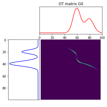
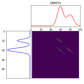
Figure 1: Transport plans between two mixtures of Gaussians $\mu_{0}$ (in blue) and $\mu_{1}$ (in red). Left, optimal transport plan for $W_{2}$. Right, optimal transport plan for $MW_{2}$. (The values on the x-axes have been mutiplied by $100$). These examples have been computed using the Python Optimal Transport (POT) library [15].

4.4 Metric properties of $MW_{2}$ and displacement interpolation

4.4.1 Metric properties of $MW_{2}$

Proposition 5.

$MW_{2}$ defines a metric on $GMM_{d}(\infty)$ and the space $GMM_{d}(\infty)$ equipped with the distance $MW_{2}$ is a geodesic space.

This proposition can be proved very easily by making use of the discrete formulation (16) of the distance (see for instance [7]). For the sake of completeness, we provide in the following a proof of the proposition using only the continuous formulation of $MW_{2}$.

Proof 4.3.

First, observe that $MW_{2}$ is obviously symmetric and positive. It is also clear that for any Gaussian mixture $\mu$, $MW_{2}(\mu,\mu)=0$. Conversely, assume that $MW_{2}(\mu_{0},\mu_{1})=0$, it implies that $W_{2}(\mu_{0},\mu_{1})=0$ and thus $\mu_{0}=\mu_{1}$ since $W_{2}$ is a distance.

It remains to show that $MW_{2}$ satisfies the triangle inequality. This is a classical consequence of the gluing lemma, but we must be careful to check that the constructed measure remains a Gaussian mixture. Let $\mu_{0},\mu_{1},\mu_{2}$ be three Gaussian mixtures on $\mathbb{R}^{d}$. Let $\gamma_{01}$ and $\gamma_{12}$ be optimal plans respectively for $(\mu_{0},\mu_{1})$ and $(\mu_{1},\mu_{2})$ for the problem $MW_{2}$ (which means that $\gamma_{01}$ and $\gamma_{12}$ are both GMM on $\mathbb{R}^{2d}$). The classical gluing lemma consists in disintegrating $\gamma_{01}$ and $\gamma_{12}$ into

$$d\gamma_{01}(y_{0},y_{1})=d\gamma_{01}(y_{0}|y_{1})d\mu_{1}(y_{1})\quad\text{and}\quad d\gamma_{12}(y_{1},y_{2})=d\gamma_{12}(y_{2}|y_{1})d\mu_{1}(y_{1}),$$

and to define

$$d\gamma_{012}(y_{0},y_{1},y_{2})=d\gamma_{01}(y_{0}|y_{1})d\mu_{1}(y_{1})d\gamma_{12}(y_{2}|y_{1}),$$

which boils down to assume independence conditionnally to the value of $y_{1}$. Since $\gamma_{01}$ and $\gamma_{12}$ are Gaussian mixtures on $\mathbb{R}^{2d}$, the conditional distributions $d\gamma_{01}(y_{0}|y_{1})$ and $d\gamma_{12}(y_{2}|y_{1})$ are also Gaussian mixtures for all $y_{1}$ in the support of $\mu_{1}$ (recalling that $\mu_{1}$ is the marginal on $y_{1}$ of both $\gamma_{01}$ and $\gamma_{12}$). If we define a distribution $\gamma_{02}$ by integrating $\gamma_{012}$ over the variable $y_{1}$, i.e.

$$d\gamma_{02}(y_{0},y_{2})=\int_{y_{1}\in\mathbb{R}^{d}}d\gamma_{012}(y_{0},y_{1},y_{2})=\int_{y_{1}\in\mathrm{Supp}(\mu_{1})}d\gamma_{01}(y_{0}|y_{1})d\mu_{1}(y_{1})d\gamma_{12}(y_{2}|y_{1})$$

then $\gamma_{02}$ is obviously also a Gaussian mixture on $\mathbb{R}^{2d}$ with marginals $\mu_{0}$ and $\mu_{2}$. The rest of the proof is classical. Indeed, we can write

$$MW_{2}^{2}(\mu_{0},\mu_{2}) \leq\int_{\mathbb{R}^{d}\times\mathbb{R}^{d}}\|y_{0}-y_{2}\|^{2}d\gamma_{02}(y_{0},y_{2})=\int_{\mathbb{R}^{d}\times\mathbb{R}^{d}\times\mathbb{R}^{d}}\|y_{0}-y_{2}\|^{2}d\gamma_{012}(y_{0},y_{1},y_{2}).$$

Writing $\|y_{0}-y_{2}\|^{2}=\|y_{0}-y_{1}\|^{2}+\|y_{1}-y_{2}\|^{2}+2\langle y_{0}-y_{1},y_{1}-y_{2}\rangle$ (with $\langle\;,\;\rangle$ the Euclidean scalar product on $\mathbb{R}^{d}$), and using the Cauchy-Schwarz inequality, it follows that

$$MW_{2}^{2}(\mu_{0},\mu_{2}) \leq\left(\sqrt{\int_{\mathbb{R}^{2d}}\|y_{0}-y_{1}\|^{2}d\gamma_{01}(y_{0},y_{1})}+\sqrt{\int_{\mathbb{R}^{2d}}\|y_{1}-y_{2}\|^{2}d\gamma_{12}(y_{1},y_{2})}\right)^{2}.$$

The triangle inequality follows by taking for $\gamma_{01}$ (resp. $\gamma_{12}$) the optimal plan for $MW_{2}$ between $\mu_{0}$ and $\mu_{1}$ (resp. $\mu_{1}$ and $\mu_{2}$).

Now, let us show that $GMM_{d}(\infty)$ equipped with the distance $MW_{2}$ is a geodesic space. For a path $\rho=(\rho_{t})_{t\in[0,1]}$ in $GMM_{d}(\infty)$ (meaning that each $\rho_{t}$ is a GMM on $\mathbb{R}^{d}$), we can define its length for $MW_{2}$ by

$$\mathrm{Len}_{MW_{2}}(\rho)=\mathrm{Sup}_{N;0=t_{0}\leq t_{1}...\leq t_{N}=1}\quad\sum_{i=1}^{N}MW_{2}(\rho_{t_{i-1}},\rho_{t_{i}})\in[0,+\infty].$$

Let $\mu_{0}=\sum_{k}\pi_{0}^{k}\mu_{0}^{k}$ and $\mu_{1}=\sum_{l}\pi_{1}^{l}\mu_{1}^{l}$ be two GMM. Since $MW_{2}$ satifies the triangle inequality, we always have that $\mathrm{Len}_{MW_{2}}(\rho)\geq MW_{2}(\mu_{0},\mu_{1})$ for all paths $\rho$ such that $\rho_{0}=\mu_{0}$ and $\rho_{1}=\mu_{1}$. To prove that $(GMM_{d}(\infty),MW_{2})$ is a geodesic space we just have to exhibit a path $\rho$ connecting $\mu_{0}$ to $\mu_{1}$ and such that its length is equal to $MW_{2}(\mu_{0},\mu_{1})$.

We write $\gamma^{\ast}$ the optimal transport plan between $\mu_{0}$ and $\mu_{1}$. For $t\in(0,1)$ we can define

$$\mu_{t}=(\mathrm{P}_{t})\#\gamma^{\ast}.$$

Let $t<s\in[0,1]$ and define $\gamma_{t,s}^{\ast}=(\mathrm{P}_{t},\mathrm{P}_{s})\#\gamma^{\ast}$. Then $\gamma_{t,s}^{\ast}\in\Pi(\mu_{t},\mu_{s})\cap GMM_{2d}(\infty)$ and therefore

$$MW_{2}(\mu_{t},\mu_{s})^{2} =\min_{\widetilde{\gamma}\in\Pi(\mu_{t},\mu_{s})\cap GMM_{2d}(\infty)}\iint\|y_{0}-y_{1}\|^{2}\,d\widetilde{\gamma}(y_{0},y_{1})$$

$$\leq\iint\|y_{0}-y_{1}\|^{2}\,d\gamma_{t,s}^{\ast}(y_{0},y_{1})=\iint\|\mathrm{P}_{t}(y_{0},y_{1})-\mathrm{P}_{s}(y_{0},y_{1})\|^{2}\,d\gamma^{\ast}(y_{0},y_{1})$$

$$=\iint\|(1-t)y_{0}+ty_{1}-(1-s)y_{0}-sy_{1}\|^{2}\,d\gamma^{\ast}(y_{0},y_{1})$$

$$=(s-t)^{2}MW_{2}(\mu_{0},\mu_{1})^{2}.$$

Thus we have that $MW_{2}(\mu_{t},\mu_{s})\leq(s-t)MW_{2}(\mu_{0},\mu_{1})$ Now, by the triangle inequality,

$$MW_{2}(\mu_{0},\mu_{1}) \leq MW_{2}(\mu_{0},\mu_{t})+MW_{2}(\mu_{t},\mu_{s})+MW_{2}(\mu_{s},\mu_{1})$$

$$\leq(t+s-t+1-s)MW_{2}(\mu_{0},\mu_{1}).$$

Therefore all inequalities are equalities, and $MW_{2}(\mu_{t},\mu_{s})=(s-t)MW_{2}(\mu_{0},\mu_{1})$ for all $0\leq t\leq s\leq 1$. This implies that the $MW_{2}$ length of the path $(\mu_{t})_{t}$ is equal to $MW_{2}(\mu_{0},\mu_{1})$. It allows us to conclude that $(GMM_{d}(\infty),MW_{2})$ is a geodesic space, and we have also given the explicit expression of the geodesic.

The following Corollary is a direct consequence of the previous results.

Corollary 2.

The barycenters between $\mu_{0}=\sum_{k}\pi_{0}^{k}\mu_{0}^{k}$ and $\mu_{1}=\sum_{l}\pi_{1}^{l}\mu_{1}^{l}$ all belong to $GMM_{d}(\infty)$ and can be written explicitely as

$$\forall t\in[0,1],\quad\mu_{t}=\mathrm{P}_{t}\#\gamma^{\ast}=\sum_{k,l}w^{\ast}_{k,l}\mu_{t}^{k,l},$$

where $w^{\ast}$ is an optimal solution of (16), and $\mu_{t}^{k,l}$ is the displacement interpolation between $\mu_{0}^{k}$ and $\mu_{1}^{l}$. When $\Sigma_{0}^{k}$ is non-singular, it is given by

$$\mu_{t}^{k,l}=((1-t)\mathrm{Id}+tT_{k,l})\#\mu_{0}^{k},$$

with $T_{k,l}$ the affine transport map between $\mu_{0}^{k}$ and $\mu_{1}^{l}$ given by Equation (9). These barycenters have less than $K_{0}+K_{1}-1$ components.

4.4.2 1D and 2D barycenter examples

One dimensional case

$t=0.0$ $t=0.2$ $t=0.4$ $t=0.6$ $t=0.8$ $t=1.0$
$W_{2}$

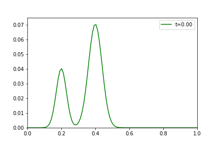
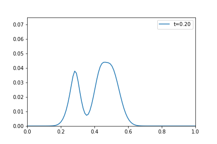
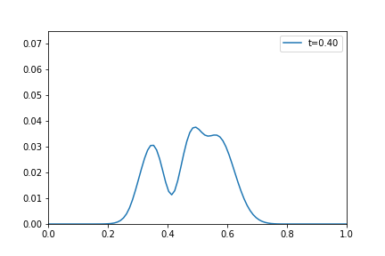
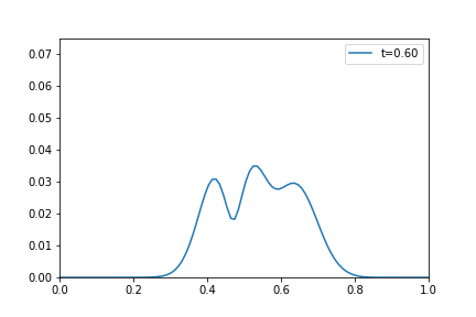
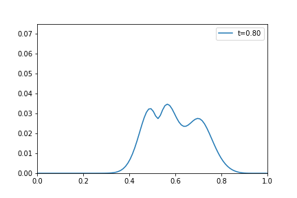
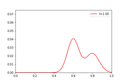
$MW_{2}$

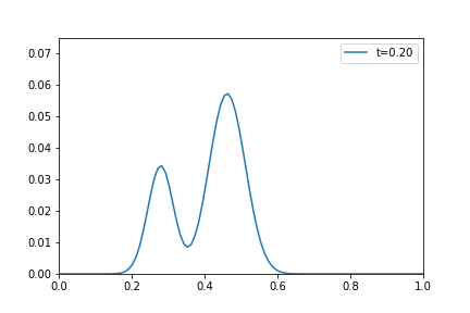
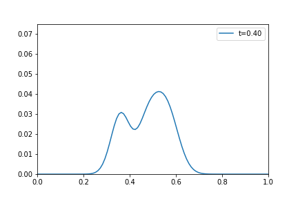
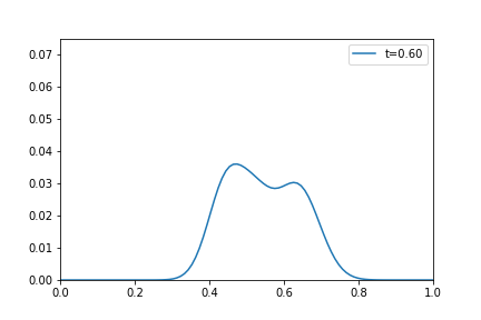
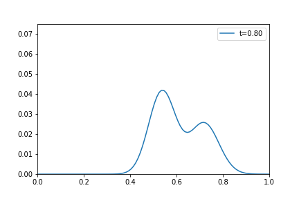
Figure 2: Barycenters $\mu_{t}$ between two Gaussian mixtures $\mu_{0}$ (green curve) and $\mu_{1}$ (red curve). Top: barycenters for the metric $W_{2}$. Bottom: barycenters for the metric $MW_{2}$. The barycenters are computed for $t=0.2,0.4,0.6,0.8$.

Figure 2 shows barycenters $\mu_{t}$ for $t=0.2,0.4,0.6,0.8$ between the $\mu_{0}$ and $\mu_{1}$ defined in Section 4.3, for both the metric $W_{2}$ and $MW_{2}$. Observe that the barycenters computed for $MW_{2}$ are a bit more regular (we know that they are mixtures of at most 3 Gaussian components) than those obtained for $W_{2}$.

Two dimensional case

$t=0.0$ $t=0.2$ $t=0.4$ $t=0.6$ $t=0.8$ $t=1.0$
$W_{2}$

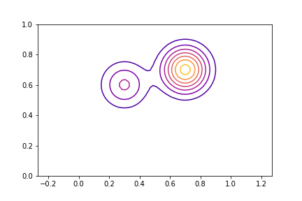
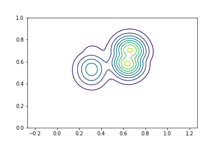
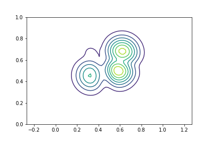
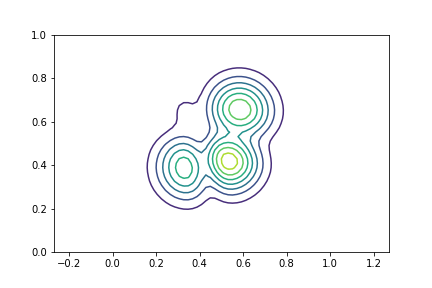
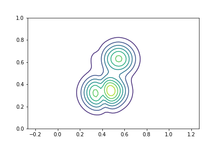
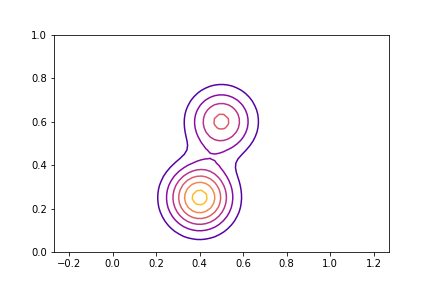
$MW_{2}$

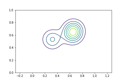
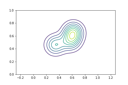
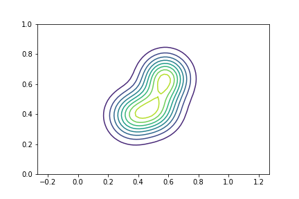
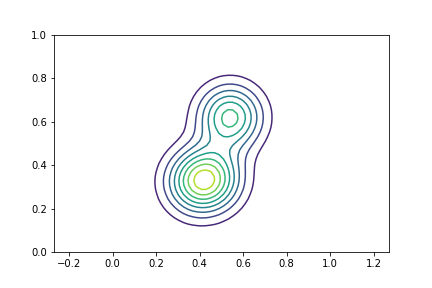
Figure 3: Barycenters $\mu_{t}$ between two Gaussian mixtures $\mu_{0}$ (first column) and $\mu_{1}$ (last column). Top: barycenters for the metric $W_{2}$. Bottom: barycenters for the metric $MW_{2}$. The barycenters are computed for $t=0.2,0.4,0.6,0.8$.

Figure 3 shows barycenters $\mu_{t}$ between the following two dimensional mixtures

$$\mu_{0}=0.3\mathcal{N}\left(\begin{pmatrix}0.3\\ 0.6\end{pmatrix},0.01I_{2}\right)+0.7\mathcal{N}\left(\begin{pmatrix}0.7\\ 0.7\end{pmatrix},0.01I_{2}\right),$$

$$\mu_{1}=0.4\mathcal{N}\left(\begin{pmatrix}0.5\\ 0.6\end{pmatrix},0.01I_{2}\right)+0.6\mathcal{N}\left(\begin{pmatrix}0.4\\ 0.25\end{pmatrix},0.01I_{2}\right),$$

where $I_{2}$ is the $2\times 2$ identity matrix. Notice that the $MW_{2}$ geodesic looks much more regular, each barycenter is a mixture of less than three Gaussians.

4.5 Comparison between $MW_{2}$ and $W_{2}$

Proposition 6.

Let $\mu_{0}\in GMM_{d}(K_{0})$ and $\mu_{1}\in GMM_{d}(K_{1})$ be two Gaussian mixtures, written as in (12). Then,

$$W_{2}(\mu_{0},\mu_{1})\leq MW_{2}(\mu_{0},\mu_{1})\leq W_{2}(\mu_{0},\mu_{1})+\sum_{i=0,1}\left(2\sum_{k=1}^{K_{i}}\pi_{i}^{k}\mathrm{trace}(\Sigma_{i}^{k})\right)^{\frac{1}{2}}.$$

The left-hand side inequality is attained when for instance

• $\mu_{0}$ and $\mu_{1}$ are both composed of only one Gaussian component,

• $\mu_{0}$ and $\mu_{1}$ are finite linear combinations of Dirac masses,

• $\mu_{1}$ is obtained from $\mu_{0}$ by an affine transformation.

As we already noticed it, the first inequality is obvious and follows from the definition of $MW_{2}$. It might not be completely intuitive that $MW_{2}$ can indeed be strictly larger than $W_{2}$ because of the density property of $GMM_{d}(\infty)$ in $\mathcal{P}_{2}(\mathbb{R}^{d})$. This follows from the fact that our optimization problem has constraints $\gamma\in\Pi(\mu_{0},\mu_{1})$. Even if any measure $\gamma$ in $\Pi(\mu_{0},\mu_{1})$ can be approximated by a sequence of Gaussian mixtures, this sequence of Gaussian mixtures will generally not belong to $\Pi(\mu_{0},\mu_{1})$, hence explaining the difference between $MW_{2}$ and $W_{2}$.

In order to show that $MW_{2}$ is always smaller than the sum of $W_{2}$ plus a term depending on the trace of the covariance matrices of the two Gaussian mixtures, we start with a lemma which makes more explicit the distance $MW_{2}$ between a Gaussian mixture and a mixture of Dirac distributions.

Lemma 4.4.

Let $\mu_{0}=\sum_{k=1}^{K_{0}}\pi_{0}^{k}\mu_{0}^{k}$ with $\mu_{0}^{k}=\mathcal{N}(m_{0}^{k},\Sigma_{0}^{k})$ and $\mu_{1}=\sum_{k=1}^{K_{1}}\pi_{1}^{k}\delta_{m_{1}^{k}}$. Let $\tilde{\mu}_{0}=\sum_{k=1}^{K_{0}}\pi_{0}^{k}\delta_{m_{0}^{k}}$ ($\tilde{\mu}_{0}$ only retains the means of $\mu_{0}$). Then,

$$MW_{2}^{2}(\mu_{0},\mu_{1})=W_{2}^{2}(\tilde{\mu}_{0},\mu_{1})+\sum_{k=1}^{K_{0}}\pi_{0}^{k}\mathrm{trace}(\Sigma_{0}^{k}).$$

Proof 4.5.

$$MW_{2}^{2}(\mu_{0},\mu_{1}) = \inf_{w\in\Pi(\pi_{0},\pi_{1})}\sum_{k,l}w_{kl}W_{2}^{2}(\mu_{0}^{k},\delta_{m_{1}^{l}})=\inf_{w\in\Pi(\pi_{0},\pi_{1})}\sum_{k,l}w_{kl}\left(\|m_{1}^{l}-m_{0}^{k}\|^{2}+\mathrm{trace}(\Sigma_{0}^{k})\right)$$

$$= \inf_{w\in\Pi(\pi_{0},\pi_{1})}\sum_{k,l}w_{kl}\|m_{1}^{l}-m_{0}^{k}\|^{2}+\sum_{k}\pi_{0}^{k}\mathrm{trace}(\Sigma_{0}^{k})=W_{2}^{2}(\tilde{\mu}_{0},\mu_{1})+\sum_{k=1}^{K_{0}}\pi_{0}^{k}\mathrm{trace}(\Sigma_{0}^{k}).$$

In other words, the squared distance $MW_{2}^{2}$ between $\mu_{0}$ and $\mu_{1}$ is the sum of the squared Wasserstein distance between $\tilde{\mu}_{0}$ and $\mu_{1}$ and a linear combination of the traces of the covariance matrices of the components of $\mu_{0}$. We are now in a position to show the other inequality between $MW_{2}$ and $W_{2}$.

Proof 4.6 (Proof of Proposition 6).

Let $(\mu_{0}^{n})_{n}$ and $(\mu_{1}^{n})_{n}$ be two sequences of mixtures of Dirac masses respectively converging to $\mu_{0}$ and $\mu_{1}$ in $\mathcal{P}_{2}(\mathbb{R}^{d})$. Since $MW_{2}$ is a distance,

$$MW_{2}(\mu_{0},\mu_{1}) \leq MW_{2}(\mu_{0}^{n},\mu_{1}^{n})+MW_{2}(\mu_{0},\mu_{0}^{n})+MW_{2}(\mu_{1},\mu_{1}^{n})$$

$$= W_{2}(\mu_{0}^{n},\mu_{1}^{n})+MW_{2}(\mu_{0},\mu_{0}^{n})+MW_{2}(\mu_{1},\mu_{1}^{n}).$$

We study in the following the limits of these three terms when $n\rightarrow+\infty$.

First, observe that $MW_{2}(\mu_{0}^{n},\mu_{1}^{n})=W_{2}(\mu_{0}^{n},\mu_{1}^{n})\longrightarrow_{n\rightarrow\infty}W_{2}(\mu_{0},\mu_{1})$ since $W_{2}$ is continuous on $\mathcal{P}_{2}(\mathbb{R}^{d})$.

Second, using Lemma 4.4, for $i=0,1$,

$$MW_{2}^{2}(\mu_{i},\mu_{i}^{n})=W_{2}^{2}(\tilde{\mu}_{i},\mu_{i}^{n})+\sum_{k=1}^{K_{i}}\pi_{i}^{k}\mathrm{trace}(\Sigma_{i}^{k})\longrightarrow_{n\rightarrow\infty}W_{2}^{2}(\tilde{\mu}_{i},\mu_{i})+\sum_{k=1}^{K_{i}}\pi_{i}^{k}\mathrm{trace}(\Sigma_{i}^{k}).$$

Define the measure $d\gamma(x,y)=\sum_{k=1}^{K_{i}}\pi_{i}^{k}\delta_{m_{i}^{k}}(y)g_{m_{i}^{k},\Sigma_{i}^{k}}(x)dx$, with $g_{m_{i}^{k},\Sigma_{i}^{k}}$ the probability density function of the Gaussian distribution $\mathcal{N}(m_{i}^{k},\Sigma_{i}^{k})$. The probability measure $\gamma$ belongs to $\Pi(\mu_{i},\tilde{\mu}_{i})$, so

$$W_{2}^{2}(\mu_{i},\tilde{\mu}_{i}) \leq \int\|x-y\|^{2}d\gamma(x,y)=\sum_{k=1}^{K_{i}}\pi_{i}^{k}\int_{\mathbb{R}^{d}}\|x-m_{i}^{k}\|^{2}g_{m_{i}^{k},\Sigma_{i}^{k}}(x)dx$$

$$= \sum_{k=1}^{K_{i}}\pi_{i}^{k}\mathrm{trace}(\Sigma_{i}^{k}).$$

We conclude that

$$MW_{2}(\mu_{0},\mu_{1}) \leq \lim\inf_{n\rightarrow\infty}\left(W_{2}(\mu_{0}^{n},\mu_{1}^{n})+MW_{2}(\mu_{0},\mu_{0}^{n})+MW_{2}(\mu_{1},\mu_{1}^{n})\right)$$

$$\leq W_{2}(\mu_{0},\mu_{1})+\left(W_{2}^{2}(\tilde{\mu}_{0},\mu_{0})+\sum_{k=1}^{K_{0}}\pi_{0}^{k}\mathrm{trace}(\Sigma_{0}^{k})\right)^{\frac{1}{2}}+\left(W_{2}^{2}(\tilde{\mu}_{1},\mu_{1})+\sum_{k=1}^{K_{1}}\pi_{1}^{k}\mathrm{trace}(\Sigma_{1}^{k})\right)^{\frac{1}{2}}$$

$$\leq W_{2}(\mu_{0},\mu_{1})+\left(2\sum_{k=1}^{K_{0}}\pi_{0}^{k}\mathrm{trace}(\Sigma_{0}^{k})\right)^{\frac{1}{2}}+\left(2\sum_{k=1}^{K_{1}}\pi_{1}^{k}\mathrm{trace}(\Sigma_{1}^{k})\right)^{\frac{1}{2}}.$$

This ends the proof of the proposition.

Observe that if $\mu$ is a Gaussian distribution $\mathcal{N}(m,\Sigma)$ and $\mu^{n}$ a distribution supported by a finite number of points which converges to $\mu$ in $\mathcal{P}_{2}(\mathbb{R}^{d})$, then

$$W_{2}^{2}(\mu,\mu^{n})\longrightarrow_{n\rightarrow\infty}0$$

and

$$MW_{2}(\mu,\mu^{n})=\left(W_{2}^{2}(\tilde{\mu},\mu^{n})+\mathrm{trace}(\Sigma)\right)^{\frac{1}{2}}\longrightarrow_{n\rightarrow\infty}\left(2\mathrm{trace}(\Sigma)\right)^{\frac{1}{2}}\neq 0.$$

Let us also remark that if $\mu_{0}$ and $\mu_{1}$ are Gaussian mixtures such that $\max_{k,i}\mathrm{trace}(\Sigma_{i}^{k})\leq\varepsilon$, then

$$MW_{2}(\mu_{0},\mu_{1})\leq W_{2}(\mu_{0},\mu_{1})+2\sqrt{2\varepsilon}.$$

4.6 Generalization to other mixture models

A natural question is to know if the methodology we have developped here, and that restricts the set of possible coupling measures to Gaussian mixtures, can be extended to other families of mixtures. Indeed, in the image processing litterature, as well as in many other fields, mixture models beyond Gaussian ones are widely used, such as Generalized Gaussian Mixture Models [11] or mixtures of T-distributions [29], for instance. Now, to extend our methodology to other mixtures, we need two main properties: (a) the identifiability property (that will ensure that there is a canonical way to write a distribution as a mixture); and (b) a marginal consistency property (we need all the marginal of an element of the family to remain in the same family). These two properties permit in particular to generalize the proof of Proposition 4. In order to make the discrete formulation convenient for numerical computations, we also need that the $W_{2}$ distance between any two elements of the family must be easy to compute.

Starting from this last requirement, we can consider a family of elliptical distributions, where the elements are of the form

$$\forall x\in\mathbb{R}^{d},f_{m,\Sigma}(x)=C_{h,d,\Sigma}\,h((x-m)^{t}\Sigma^{-1}(x-m)),$$

where $m\in\mathbb{R}^{d}$, $\Sigma$ is a positive definite symmetric matrix and $h$ is a given function from $[0,+\infty)$ to $[0,+\infty)$. Gaussian distributions are an example, with $h(t)=\exp(-t/2)$. Generalized Gaussian distributions are obtained with $h(t)=\exp(-t^{\beta})$, with $\beta$ not necessarily equal to $1$. T-distributions are also in this family, with $h(t)=(1+t/\nu)^{-(\nu+d)/2}$, etc. Thanks to their elliptical contoured property, the $W_{2}$ distance between two elements in such a family (i.e. $h$ fixed) can be explicitely computed (see Gelbrich [18]), and yields a formula that is the same as the one in the Gaussian case (Equation (8)). In such a family, the identifiability property can be checked, using the asymptotic behavior in all directions of $\mathbb{R}^{d}$. Now, if we want the marginal consistency property to be also satisfied (which is necessary if we want the coupling restriction problem to be well-defined), the choice of $h$ is very limited. Indeed, Kano in [21], proved that the only elliptical distributions with the marginal consistency property are the ones which are a scale mixture of normal distributions with a mixing variable that is unrelated to the dimension $d$. So, generalized Gaussian distributions don’t satisfy this marginal consistency property, but T-distributions do.

5 Multi-marginal formulation and barycenters

5.1 Multi-marginal formulation for $MW_{2}$

Let $\mu_{0},\mu_{1}\dots,\mu_{J-1}$ be $J$ Gaussian mixtures on $\mathbb{R}^{d}$, and let $\lambda_{0},\dots\lambda_{J-1}$ be $J$ positive weights summing to $1$. The multi-marginal version of our optimal transport problem restricted to Gaussian mixture models can be written

(18) $$MMW_{2}^{2}(\mu_{0},\dots,\mu_{J-1}):=\inf_{\gamma\in\Pi(\mu_{0},\dots,\mu_{J-1})\cap GMM_{Jd}(\infty)}\int_{\mathbb{R}^{dJ}}c(x_{0},\dots,x_{J-1})d\gamma(x_{0},\dots,x_{J-1}),$$

where

(19) $$c(x_{0},\dots,x_{J-1})=\sum_{i=0}^{J-1}\lambda_{i}\|x_{i}-B(x)\|^{2}=\frac{1}{2}\sum_{i,j=0}^{J-1}\lambda_{i}\lambda_{j}\|x_{i}-x_{j}\|^{2}$$

and where $\Pi(\mu_{0},\mu_{1},\dots,\mu_{J-1})$ is the set of probability measures on $(\mathbb{R}^{d})^{J}$ having $\mu_{0}$, $\mu_{1}$, $\dots$, $\mu_{J-1}$ as marginals.

Writing for every $j$, $\mu_{j}=\sum_{k=1}^{K_{j}}\pi_{j}^{k}\mu_{j}^{k}$, and using exactly the same arguments as in Proposition 4, we can easily show the following result.

Proposition 7.

The optimisation problem (18) can be rewritten under the discrete form

(20) $$MMW_{2}^{2}(\mu_{0},\dots,\mu_{J-1})=\min_{w\in\Pi(\pi_{0},\dots,\pi_{J-1})}\sum_{k_{0},\dots,k_{J-1}=1}^{K_{0},\dots,K_{J-1}}w_{k_{0}\dots k_{J-1}}mmW_{2}^{2}(\mu_{0}^{k_{0}},\dots,\mu_{J-1}^{k_{J-1}}),$$

where $\Pi(\pi_{0},\pi_{1},\dots,\pi_{J-1})$ is the subset of tensors $w$ in $\mathcal{M}_{K_{0},K_{1},\dots,K_{J-1}}(\mathbb{R}^{+})$ having $\pi_{0}$, $\pi_{1}$, $\dots$, $\pi_{J-1}$ as discrete marginals, i.e. such that

(21) $$\forall j\in\{0,\dots,J-1\},\;\forall k\in\{1,\dots,K_{j}\},\sum_{\begin{subarray}{c}1\leq k_{0}\leq K_{0}\\ \dots\\ 1\leq k_{j-1}\leq K_{j-1}\\ k_{j}=k\\ 1\leq k_{j+1}\leq K_{j+1}\\ \dots\\ 1\leq k_{J-1}\leq K_{J-1}\end{subarray}}w_{k_{0}k_{1}\dots k_{J-1}}=\pi_{j}^{k}.$$

Moreover, the solution $\gamma^{*}$ of (18) can be written

(22) $$\gamma^{*}=\sum_{\begin{subarray}{c}1\leq k_{0}\leq K_{0}\\ \dots\\ 1\leq k_{J-1}\leq K_{J-1}\end{subarray}}w^{*}_{k_{0}k_{1}\dots k_{J-1}}\gamma^{*}_{k_{0}k_{1}\dots k_{J-1}},$$

where $w^{*}$ is solution of (20) and $\gamma^{*}_{k_{0}k_{1}\dots k_{J-1}}$ is the optimal multi-marginal plan between the Gaussian measures $\mu_{0}^{k_{0}},\dots,\mu_{J-1}^{k_{J-1}}$ (see Section 2.4.2).

From Section 2.4.2, we know how to construct the optimal multi-marginal plans $\gamma^{*}_{k_{0}k_{1}\dots k_{J-1}}$, which means that computing a solution for (18) boils down to solve the linear program (20) in order to find $w^{*}$.

5.2 Link with the $MW_{2}$-barycenters

We will now show the link between the previous multi-marginal problem and the barycenters for $MW_{2}$.

Proposition 8.

The barycenter problem

(23) $$\inf_{\nu\in GMM_{d}(\infty)}\sum_{j=0}^{J-1}\lambda_{j}MW_{2}^{2}(\mu_{j},\nu),$$

has a solution given by $\nu^{*}=B\#\gamma^{*}$, where $\gamma^{*}$ is an optimal plan for the multi-marginal problem (18).

Proof 5.1.

For any $\gamma\in\Pi(\mu_{0},\dots,\mu_{J-1})\cap GMM_{Jd}(\infty)$, we define $\gamma_{j}=(P_{j},B)\#\gamma$, with $B$ the barycenter application defined in (5) and $P_{j}:(\mathbb{R}^{d})^{J}\mapsto\mathbb{R}^{d}$ such that $P(x_{0},\dots,x_{J-1})=x_{j}$. Observe that $\gamma_{j}$ belongs to $\Pi(\mu_{j},\nu)$ with $\nu=B\#\gamma$. The probability measure $\gamma_{j}$ also belongs to $GMM_{2d}(\infty)$ since $(P_{j},B)$ is a linear application. It follows that

$$\int_{(\mathbb{R}^{d})^{J}}\sum_{j=0}^{J-1}\lambda_{j}\|x_{j}-B(x)\|^{2}d\gamma(x_{0},\dots,x_{J-1}) =\sum_{j=0}^{J-1}\lambda_{j}\int_{(\mathbb{R}^{d})^{J}}\|x_{j}-B(x)\|^{2}d\gamma(x_{0},\dots,x_{J-1})$$

$$=\sum_{j=0}^{J-1}\lambda_{j}\int_{\mathbb{R}^{d}\times\mathbb{R}^{d}}\|x_{j}-y\|^{2}d\gamma_{j}(x_{j},y)$$

$$\geq\sum_{j=0}^{J-1}\lambda_{j}MW_{2}^{2}(\mu_{j},\nu).$$

This inequality holds for any arbitrary $\gamma\in\Pi(\mu_{0},\dots,\mu_{J-1})\cap GMM_{Jd}(\infty)$, thus

$$MMW_{2}^{2}(\mu_{0},\dots,\mu_{J-1})\geq\inf_{\nu\in GMM_{d}(\infty)}\sum_{j=0}^{J-1}\lambda_{j}MW_{2}^{2}(\mu_{j},\nu).$$

Conversely, for any $\nu$ in $GMM_{d}(\infty)$, we can write $\nu=\sum_{l=1}^{L}\pi_{\nu}^{l}\nu^{l}$, the $\nu^{l}$ being Gaussian probability measures. We also write $\mu_{j}=\sum_{k=1}^{K_{j}}\pi_{j}^{k}\mu_{j}^{k}$, and we call $w^{j}$ the optimal discrete plan for $MW_{2}$ between the mixtures $\mu_{j}$ and $\nu$ (see Equation (16)). Then,

$$\sum_{j=0}^{J-1}\lambda_{j}MW_{2}^{2}(\mu_{j},\nu) =\sum_{j=0}^{J-1}\lambda_{j}\sum_{k,l}w_{k,l}^{j}W_{2}^{2}(\mu_{j}^{k},\nu^{l}).$$

Now, if we define a $K_{0}\times\dots\times K_{J-1}\times L$ tensor $\alpha$ and a $K_{0}\times\dots\times K_{J-1}$ tensor $\overline{\alpha}$ by

$$\alpha_{k_{0}\dots k_{J-1}l}=\frac{\prod_{j=0}^{J-1}w_{k_{j},l}^{j}}{(\pi_{\nu}^{l})^{J-1}}\;\;\text{ and }\quad\overline{\alpha}_{k_{0}\dots k_{J-1}}=\sum_{l=1}^{L}\alpha_{k_{0}\dots k_{J-1}l},$$

clearly $\alpha\in\Pi(\pi_{0},\dots,\pi_{J-1},\pi_{\nu})$ and $\overline{\alpha}\in\Pi(\pi_{0},\dots,\pi_{J-1})$. Moreover,

$$\sum_{j=0}^{J-1}\lambda_{j}MW_{2}^{2}(\mu_{j},\nu) =\sum_{j=0}^{J-1}\lambda_{j}\sum_{k_{j}=1}^{K_{j}}\sum_{l=1}^{L}w_{k_{j},l}^{j}W_{2}^{2}(\mu_{j}^{k_{j}},\nu^{l})$$

$$=\sum_{j=0}^{J-1}\lambda_{j}\sum_{k_{0},\dots,k_{J-1},l}\alpha_{k_{0}\dots k_{J-1}l}W_{2}^{2}(\mu_{j}^{k_{j}},\nu^{l})$$

$$=\sum_{k_{0},\dots,k_{J-1},l}\alpha_{k_{0}\dots k_{J-1}l}\sum_{j=0}^{J-1}\lambda_{j}W_{2}^{2}(\mu_{j}^{k_{j}},\nu^{l})$$

$$\geq\sum_{k_{0},\dots,k_{J-1},l}\alpha_{k_{0}\dots k_{J-1}l}mmW_{2}^{2}(\mu_{0}^{k_{0}},\dots,\mu_{J-1}^{k_{J-1}})\quad\text{ (see Equation\leavevmode\nobreak\ \eqref{eq:MW2_bary})}$$

$$=\sum_{k_{0},\dots,k_{J-1}}\overline{\alpha}_{k_{0}\dots k_{J-1}}mmW_{2}^{2}(\mu_{0}^{k_{0}},\dots,\mu_{J-1}^{k_{J-1}})\geq MMW_{2}^{2}(\mu_{0},\dots,\mu_{J-1}),$$

the last inequality being a consequence of Proposition 7. Since this holds for any arbitrary $\nu$ in $GMM_{d}(\infty)$, this ends the proof.

The following corollary gives a more explicit formulation for the barycenters for $MW_{2}$, and shows that the number of Gaussian components in the mixture is much smaller than $\prod_{j=0}^{J-1}K_{j}$.

Corollary 3.

Let $\mu_{0},\dots,\mu_{J-1}$ be $J$ Gaussian mixtures such that all the involved covariance matrices are positive definite, then the solution of (23) can be written

(24) $$\nu=\sum_{k_{0},\dots,k_{J-1}}w^{*}_{k_{0}\dots k_{J-1}}\nu_{k_{0}\dots k_{J-1}}$$

where $\nu_{k_{0}\dots k_{J-1}}$ is the Gaussian barycenter for $W_{2}$ between the components $\mu_{0}^{k_{0}},\dots,\mu_{J-1}^{k_{J-1}}$, and $w^{*}$ is the optimal solution of (20). Moreover, this barycenter has less than $K_{0}+\dots+K_{J-1}-J+1$ non-zero coefficients.

Proof 5.2.

This follows directly from the proof of the previous propositions. The linear program (20) has $K_{0}+\dots+K_{J-1}-J+1$ affine constraints, and thus must have at least a solution with less than $K_{0}+\dots+K_{J-1}-J+1$ components.

To conclude this section, it is important to emphasize that the problem of barycenters for the distance $MW_{2}$, as defined in (23), is completely different from

(25) $$\inf_{\nu\in GMM_{d}(\infty)}\sum_{j=0}^{J-1}\lambda_{j}W_{2}^{2}(\mu_{j},\nu).$$

Indeed, since $GMM_{d}(\infty)$ is dense in $\mathcal{P}_{2}(\mathbb{R}^{d})$ and the total cost on the right is continuous on $\mathcal{P}_{2}(\mathbb{R}^{d})$, the infimum in (25) is exactly the same as the infimum over $\mathcal{P}_{2}(\mathbb{R}^{d})$. Even if the barycenter for $W_{2}$ is not a mixture itself, it can be approximated by a sequence of Gaussian mixtures with any desired precision. Of course, these mixtures might have a very high number of components in practice.

5.3 Some examples

The previous propositions give us a very simple way to compute barycenters between Gaussian mixtures for the metric $MW_{2}$. For given mixtures $\mu_{0},\dots,\mu_{J-1}$, we first compute all the values $mmW_{2}(\mu_{0}^{k_{0}},\dots,\mu_{J-1}^{k_{J-1}})$ between their components (and these values can be computed iteratively, see Section 2.4.2) and the corresponding Gaussian barycenters $\nu_{k_{0}\dots k_{J-1}}$. Then we solve the linear program (20) to find $w^{*}$.

Figure 4 shows the barycenters between the following simple two dimensional mixtures

$$\mu_{0}= \frac{1}{3}\mathcal{N}\left(\begin{pmatrix}0.5\\ 0.75\end{pmatrix},0.025\begin{pmatrix}0.1&0\\ 0&0.05\end{pmatrix}\right)+\frac{1}{3}\mathcal{N}\left(\begin{pmatrix}0.5\\ 0.25\end{pmatrix},0.025\begin{pmatrix}0.1&0\\ 0&0.05\end{pmatrix}\right)$$

$$+\frac{1}{3}\mathcal{N}\left(\begin{pmatrix}0.5\\ 0.5\end{pmatrix},0.025\begin{pmatrix}0.06&0\\ 0.05&0.05\end{pmatrix}\right),$$

$$\mu_{1}= \frac{1}{4}\mathcal{N}\left(\begin{pmatrix}0.25\\ 0.25\end{pmatrix},0.01I_{2}\right)+\frac{1}{4}\mathcal{N}\left(\begin{pmatrix}0.75\\ 0.75\end{pmatrix},0.01I_{2}\right)+\frac{1}{4}\mathcal{N}\left(\begin{pmatrix}0.7\\ 0.25\end{pmatrix},0.01I_{2}\right)$$

$$+\frac{1}{4}\mathcal{N}\left(\begin{pmatrix}0.25\\ 0.75\end{pmatrix},0.01I_{2}\right),$$

$$\mu_{2}= \frac{1}{4}\mathcal{N}\left(\begin{pmatrix}0.5\\ 0.75\end{pmatrix},0.025\begin{pmatrix}1&0\\ 0&0.05\end{pmatrix}\right)+\frac{1}{4}\mathcal{N}\left(\begin{pmatrix}0.5\\ 0.25\end{pmatrix},0.025\begin{pmatrix}1&0\\ 0&0.05\end{pmatrix}\right)$$

$$+\frac{1}{4}\mathcal{N}\left(\begin{pmatrix}0.25\\ 0.5\end{pmatrix},0.025\begin{pmatrix}0.05&0\\ 0&1\end{pmatrix}\right)+\frac{1}{4}\mathcal{N}\left(\begin{pmatrix}0.75\\ 0.5\end{pmatrix},0.025\begin{pmatrix}0.05&0\\ 0&1\end{pmatrix}\right),$$

$$\mu_{3}= \frac{1}{3}\mathcal{N}\left(\begin{pmatrix}0.8\\ 0.7\end{pmatrix},0.01\begin{pmatrix}2&0\\ 1&1\end{pmatrix}\right)+\frac{1}{3}\mathcal{N}\left(\begin{pmatrix}0.2\\ 0.7\end{pmatrix},0.01\begin{pmatrix}2&0\\ -1&1\end{pmatrix}\right)$$

$$+\frac{1}{3}\mathcal{N}\left(\begin{pmatrix}0.5\\ 0.3\end{pmatrix},0.01\begin{pmatrix}6&0\\ 0&1\end{pmatrix}\right),$$

where $I_{2}$ is the $2\times 2$ identity matrix. Each barycenter is a mixture of at most $K_{0}+K_{1}+K_{2}+K_{3}-4+1=11$ components. By thresholding the mixtures densities, this yields barycenters between 2-D shapes.

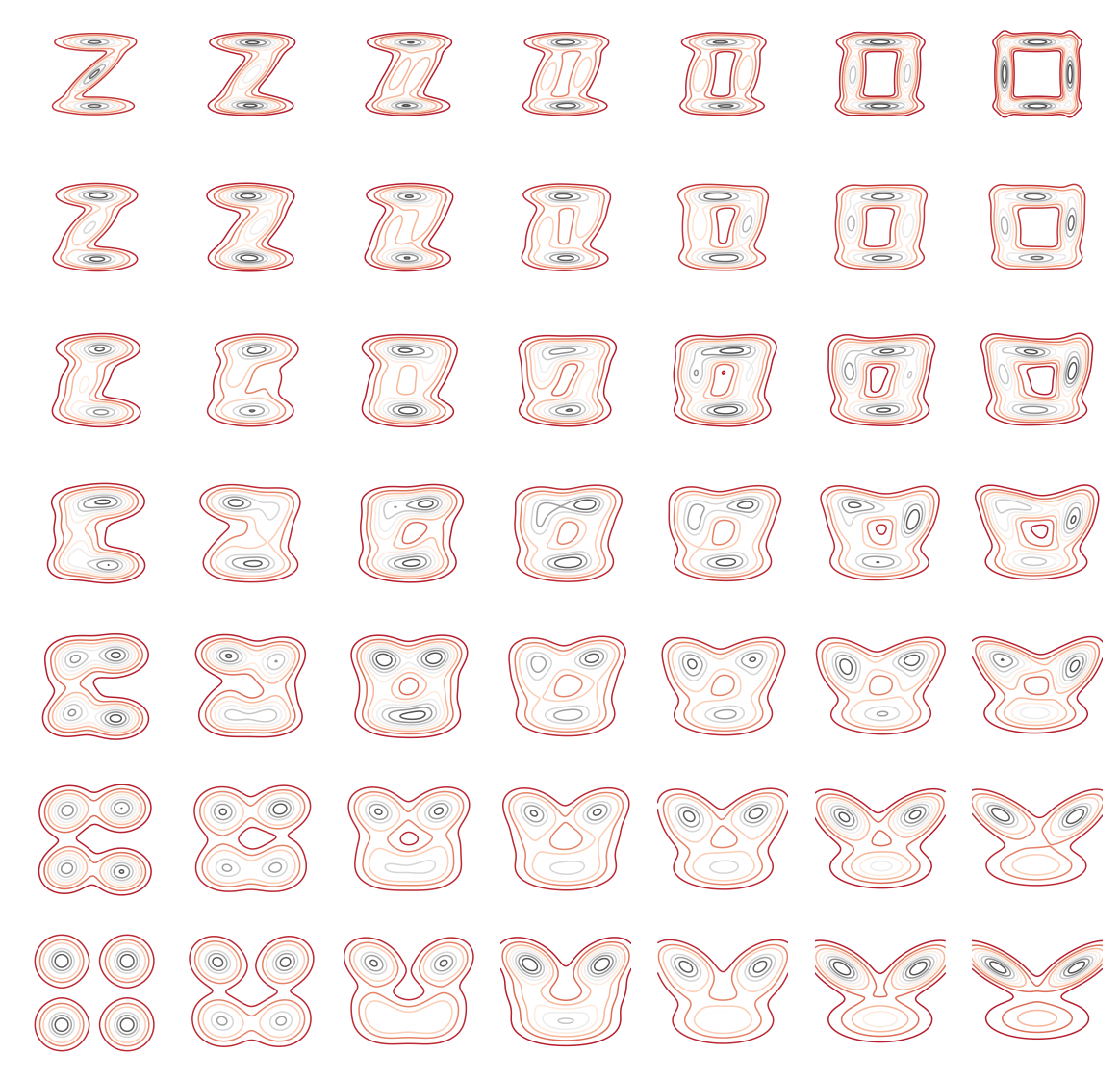
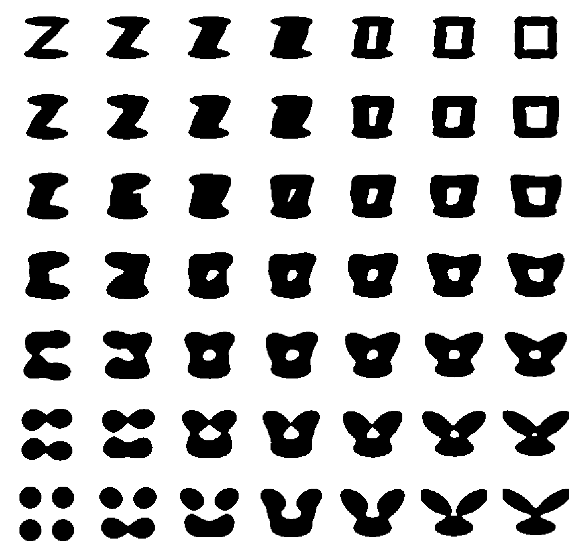
Figure 4: $MW_{2}$-barycenters between 4 Gaussian mixtures $\mu_{0}$, $\mu_{1}$, $\mu_{2}$ and $\mu_{3}$. On the left, some level sets of the distributions are displayed. On the right, densities thresholded at level $1$ are displayed. We use bilinear weights with respect to the four corners of the square.

To go further, Figure 5 shows barycenters where more involved shapes have been approximated by mixtures of 12 Gaussian components each. Observe that, even if some of the original shapes (the star, the cross) have symmetries, these symmetries are not necessarily respected by the estimated GMM, and thus not preserved in the barycenters. This could be easily solved by imposing some symmetry in the GMM estimation for these shapes.

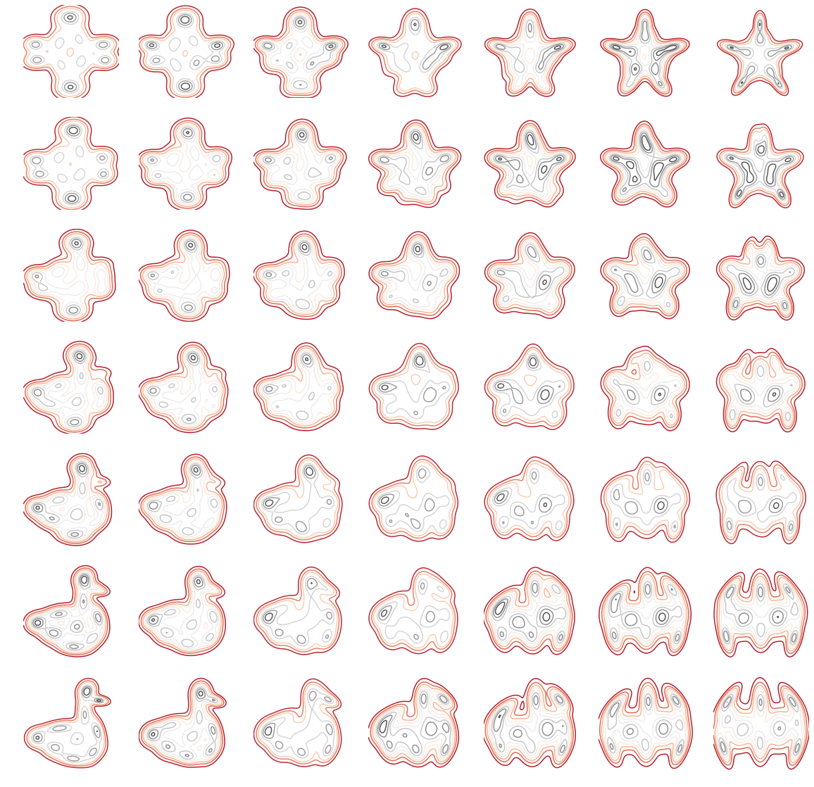
Figure 5: Barycenters between four mixtures of 12 Gaussian components, $\mu_{0}$, $\mu_{1}$, $\mu_{2}$, $\mu_{3}$ for the metric $MW_{2}$. The weights are bilinear with respect to the four corners of the square.

6 Using $MW_{2}$ in practice

6.1 Extension to probability distributions that are not GMM

Most applications of optimal transport involve data that do not follow a Gaussian mixture model and we can wonder how to make use of the distance $MW_{2}$ and the corresponding transport plans in this case. A simple solution is to approach these data by convenient Gaussian mixture models and to use the transport plan $\gamma$ (or one of the maps defined in the previous section) to displace the data.

Given two probability measures $\nu_{0}$ and $\nu_{1}$, we can define a pseudo-distance $MW_{K,2}(\nu_{0},\nu_{1})$ as the distance $MW_{2}({\mu}_{0},{\mu}_{1})$, where each ${\mu}_{i}$ ($i=0,1$) is the Gaussian mixture model with $K$ components which minimizes an appropriate “similarity measure” to $\nu_{i}$. For instance, if $\nu_{i}$ is a discrete measure $\nu_{i}=\frac{1}{J_{i}}\sum_{j=1}^{J_{i}}\delta_{x^{i}_{j}}$ in $\mathbb{R}^{d}$ , this similarity can be chosen as the opposite of the log-likelihood of the discrete set of points $\{x_{j}\}_{j=1,\dots,J_{i}}$ and the parameters of the Gaussian mixture can be infered thanks to the Expectation-Maximization algorithm. Observe that this log-likelihood can also be written

$$\mathbb{E}_{\nu_{i}}[\log{\mu}_{i}].$$

If $\nu_{i}$ is absolutely continuous, we can instead choose ${\mu}_{i}$ which minimizes $\mathrm{KL}(\nu_{i},{\mu}_{i})$ among GMM of order $K$. The discrete and continuous formulations coincide since

$$\mathrm{KL}(\nu_{i},{\mu}_{i})=-H(\nu_{i})-\mathbb{E}_{\nu_{i}}[\log{\mu}_{i}],$$

where $H(\nu_{i})$ is the differential entropy of $\nu_{i}$.

In both cases, the corresponding $MW_{K,2}$ does not define a distance since two different distributions may have the same corresponding Gaussian mixture. However, for $K$ large enough, their approximation by Gaussian mixtures will become different. The choice of $K$ must be a compromise between the quality of the approximation given by Gaussian mixture models and the affordable computing time. In any case, the optimal transport plan $\gamma_{K}$ involved in $MW_{2}({\mu}_{0},{\mu}_{1})$ can be used to compute an approximate transport map between $\nu_{0}$ and $\nu_{1}$.

In the experimental section, we will use this approximation for different data, generally with $K=10$.

6.2 A similarity measure mixing $MW_{2}$ and $KL$

In the previous paragraphs, we have seen how to use our Wasserstein-type distance $MW_{2}$ and its associated optimal transport plan on probability measures $\nu_{0}$ and $\nu_{1}$ that are not GMM. Instead of a two step formulation (first an approximation by two GMM, and second the computation of $MW_{2}$), we propose here a relaxed formulation combining directly $MW_{2}$ with the Kullback-Leibler divergence.

Let $\nu_{0}$ and $\nu_{1}$ be two probability measures on $\mathbb{R}^{d}$, we define

(26) $$E_{K,\lambda}(\nu_{0},\nu_{1})=\min_{\gamma\in GMM_{2d}(K)}\int_{\mathbb{R}^{d}\times\mathbb{R}^{d}}\|y_{0}-y_{1}\|^{2}d\gamma(y_{0},y_{1})-\lambda\mathbb{E}_{\nu_{0}}[\log P_{0}\#\gamma]-\lambda\mathbb{E}_{\nu_{1}}[\log P_{1}\#\gamma],$$

where $\lambda>0$ is a parameter.

In the case where $\nu_{0}$ and $\nu_{1}$ are absolutely continuous with respect to the Lebesgue measure, we can write instead

(27) $$\widetilde{E_{K,\lambda}}(\nu_{0},\nu_{1})=\min_{\gamma\in GMM_{2d}(K)}\int_{\mathbb{R}^{d}\times\mathbb{R}^{d}}\|y_{0}-y_{1}\|^{2}d\gamma(y_{0},y_{1})+\lambda\mathrm{KL}(\nu_{0},P_{0}\#\gamma)+\lambda\mathrm{KL}(\nu_{1},P_{1}\#\gamma)$$

and $\widetilde{E_{K,\lambda}}(\nu_{0},\nu_{1})=E_{K,\lambda}(\nu_{0},\nu_{1})-\lambda H(\nu_{0})-\lambda H(\nu_{1}).$ Note that this formulation does not define a distance in general.

This formulation is close to the unbalanced formulation of optimal transport proposed by Chizat et al. in [10], with two differences: a) we constrain the solution $\gamma$ to be a GMM; and b) we use $\mathrm{KL}(\nu_{0},P_{0}\#\gamma)$ instead of $\mathrm{KL}(P_{0}\#\gamma,\nu_{0})$. In their case, the support of $P_{i}\#\gamma$ must be contained in the support of $\nu_{i}$. When $\nu_{i}$ has a bounded support, this constraint is quite strong and would not make sense for a GMM $\gamma$.

For discrete measures $\nu_{0}$ and $\nu_{1}$, when $\lambda$ goes to infinity, minimizing (26) becomes equivalent to approximate $\nu_{0}$ and $\nu_{1}$ by the EM algorithm and this only imposes the marginals of $\gamma$ to be as close as possible to $\nu_{0}$ and $\nu_{1}$. When $\lambda$ decreases, the first term favors solutions $\gamma$ whose marginals become closer.

Solving this problem (Equation (26)) leads to computations similar to those used in the EM iterations [4]. By differentiating with respect to the weights, means and covariances of $\gamma$, we obtain equations which are not in closed-form. For the sake of simplicity, we illustrate here what happens in one dimension.
Let $\gamma\in GMM_{2}(K)$ be a Gaussian mixture in dimension $2d=2$ with $K$ elements. We write

$$\gamma=\sum_{k=1}^{K}\pi_{k}\mathcal{N}\left(\left(\begin{array}[]{c}m_{0,k}\\ m_{1,k}\end{array}\right),\left(\begin{array}[]{cc}\sigma_{0,k}^{2}&a_{k}\\ a_{k}&\sigma_{1,k}^{2}\end{array}\right)\right).$$

We have that the marginals are given by the 1d Gaussian mixtures

$$P_{0}\#\gamma=\sum_{k=1}^{K}\pi_{k}\mathcal{N}(m_{0,k},\sigma_{0,k}^{2})\quad\text{ and }\quad P_{1}\#\gamma=\sum_{k=1}^{K}\pi_{k}\mathcal{N}(m_{1,k},\sigma_{1,k}^{2}).$$

Then, to minimize, with respect to $\gamma$, the energy $E_{K,\lambda}(\nu_{0},\nu_{1})$ above, since the $\mathrm{KL}$ terms are independent of the $a_{k}$, we can directly take $a_{k}=\sigma_{0,k}\sigma_{1,k}$, and the transport cost term becomes

$$\int_{\mathbb{R}^{d}\times\mathbb{R}^{d}}\|y_{0}-y_{1}\|^{2}d\gamma(y_{0},y_{1})=\sum_{k=1}^{K}\pi_{k}\left[(m_{0,k}-m_{1,k})^{2}+(\sigma_{0,k}-\sigma_{1,k})^{2}\right].$$

Therefore, we have to consider the problem of minimizing the following “energy”:

$$F(\gamma) = \sum_{k=1}^{K}\pi_{k}\left[(m_{0,k}-m_{1,k})^{2}+(\sigma_{0,k}-\sigma_{1,k})^{2}\right]$$

$$-\lambda\int_{\mathbb{R}}\log\left(\sum_{k=1}^{K}\pi_{k}g_{m_{0,k},\sigma_{0,k}^{2}}(x)\right)d\nu_{0}(x)-\lambda\int_{\mathbb{R}}\log\left(\sum_{k=1}^{K}\pi_{k}g_{m_{1,k},\sigma_{1,k}^{2}}(x)\right)d\nu_{1}(x).$$

It can be optimized through a simple gradient descent on the parameters $\pi_{k}$, $m_{i,k}$, $\sigma_{i,k}$ for $i=0,1$ and $k=1,\ldots,K$. Indeed a simple calculus shows that we can write

$$\frac{\partial F(\gamma)}{\partial\pi_{k}}=\left[(m_{0,k}-m_{1,k})^{2}+(\sigma_{0,k}-\sigma_{1,k})^{2}\right]-\lambda\frac{\tilde{\pi}_{0,k}+\tilde{\pi}_{1,k}}{\pi_{k}},$$

$$\frac{\partial F(\gamma)}{\partial m_{i,k}}=2\pi_{k}(m_{i,k}-m_{i,k})-\lambda\frac{\tilde{\pi}_{i,k}}{\sigma_{i,k}^{2}}(\tilde{m}_{i,k}-m_{i,k}),$$

$$\text{ and }\quad\frac{\partial F(\gamma)}{\partial\sigma_{i,k}}=2\pi_{k}(\sigma_{i,k}-\sigma_{j,k})-\lambda\frac{\tilde{\pi}_{i,k}}{\sigma_{i,k}^{3}}(\tilde{\sigma}_{i,k}^{2}-\sigma_{i,k}^{2}),$$

where we have introduced some auxilary empirical estimates of the variables given, for $i=0,1$ and $k=1,\ldots,K$, by

$$\gamma_{i,k}(x)=\frac{\pi_{k}g_{m_{i,k},\sigma_{i,k}^{2}}(x)}{\sum_{l=1}^{K}\pi_{l}g_{m_{i,l},\sigma_{i,l}^{2}}(x)}\quad\text{ and }\quad\tilde{\pi}_{i,k}=\int\gamma_{i,k}(x)d\nu_{i}(x);$$

$$\tilde{m}_{i,k}=\frac{1}{\tilde{\pi}_{i,k}}\int x\gamma_{i,k}(x)d\nu_{i}(x)\quad\text{ and }\quad\tilde{\sigma}_{i,k}^{2}=\frac{1}{\tilde{\pi}_{i,k}}\int(x-m_{i,k})^{2}\gamma_{i,k}(x)d\nu_{i}(x).$$

Automatic differenciation of $F$ can also be used in practice. At each iteration of the gradient descent, we project on the constraints $\pi_{k}\geq 0$, $\sigma_{i,k}\geq 0$ and $\sum_{k}\pi_{k}=1$.

On Figure 6, we illustrate this approach on a simple example. The distributions $\nu_{0}$ and $\nu_{1}$ are 1d discrete distributions, plotted as the red and blue histograms. On this example, we choose $K=3$ and we use automatic differenciation (with the torch.autograd Python library) for the sake of convenience. The red and blue plain curves represent the final distributions $P_{0}\#\gamma$ and $P_{1}\#\gamma$, for $\lambda$ in the set $\{10,2,1,0.5,0.1,0.01\}$. The behavior is as expected: when $\lambda$ is large, the KL terms are dominating and the distribution $\gamma$ tends to have its marginal fitting well the two distributions $\nu_{0}$ and $\nu_{1}$. Whereas, when $\lambda$ is small, the Wasserstein transport term dominates and the two marginals of $\gamma$ are almost equal.

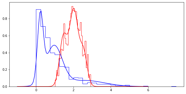
(a) $\lambda=10$

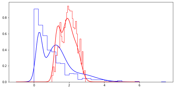
(b) $\lambda=2$

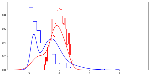
(c) $\lambda=1$

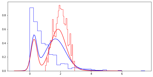
(d) $\lambda=0.5$

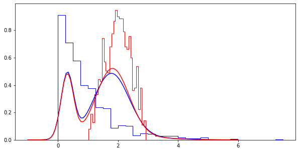
(e) $\lambda=0.1$

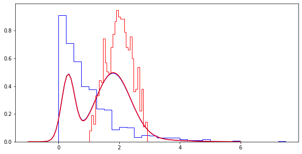
(f) $\lambda=0.01$

Figure 6: The distributions $\nu_{0}$ and $\nu_{1}$ are 1d discrete distributions, plotted as the red and blue discrete histograms. The red and blue plain curves represent the final distributions $P_{0}\#\gamma$ and $P_{1}\#\gamma$. In this experiment, we use $K=3$ Gaussian components for $\gamma$.

6.3 From a GMM transport plan to a transport map

Usually, we need not only to have an optimal transport plan and its corresponding cost, but also an assignment giving for each $x\in\mathbb{R}^{d}$ a corresponding value $T(x)\in\mathbb{R}^{d}$. Let $\mu_{0}$ and $\mu_{1}$ be two GMM. Then, the optimal transport plan between $\mu_{0}$ and $\mu_{1}$ for $MW_{2}$ is given by

$$\gamma(x,y)=\sum_{k,l}w_{k,l}^{\ast}g_{m_{0}^{k},\Sigma_{0}^{k}}(x)\delta_{y=T_{k,l}(x)}.$$

It is not of the form $(\mathrm{Id},T)\#\mu_{0}$ (see also Figure 1 for an example), but we can however define a unique assignment of each $x$, for instance by setting

$$T_{mean}(x)=\mathbb{E}_{\gamma}(Y|X=x),$$

where here $(X,Y)$ is distributed according to the probability distribution $\gamma$. Then, since the distribution of $Y|X=x$ is given by the discrete distribution

$$\sum_{k,l}p_{k,l}(x)\delta_{T_{k,l}(x)}\quad\text{ with }\quad p_{k,l}(x)=\frac{w_{k,l}^{\ast}g_{m_{0}^{k},\Sigma_{0}^{k}}(x)}{\sum_{j}\pi_{0}^{j}g_{m_{0}^{j},\Sigma_{0}^{j}}(x)},$$

we get that

$$T_{mean}(x)=\frac{\sum_{k,l}w_{k,l}^{\ast}g_{m_{0}^{k},\Sigma_{0}^{k}}(x)T_{k,l}(x)}{\sum_{k}\pi^{k}_{0}g_{m_{0}^{k},\Sigma_{0}^{k}}(x)}.$$

Notice that the $T_{mean}$ defined this way is an assignment that will not necessarily satisfy the properties of an optimal transport map. In particular, in dimension $d=1$, the map $T_{mean}$ may not be increasing: each $T_{k,l}$ is increasing but because of the weights that depend on $x$, their weighted sum is not necessarily increasing. Another issue is that $T_{mean}\#\mu_{0}$ may be “far” from the target distribution $\mu_{1}$. This happens for instance, in 1D, when $\mu_{0}=\mathcal{N}(0,1)$ and $\mu_{1}$ is the mixture of $\mathcal{N}(-a,1)$ and $\mathcal{N}(a,1)$, each with weight $0.5$. In this extreme case we even have that $T_{mean}$ is the identity map, and thus $T_{mean}\#\mu_{0}=\mu_{0}$, that can be very far from $\mu_{1}$ when $a$ is large.

Now, another way to define an assignment is to define it as a random assignment using the optimal plan $\gamma$. More precisely, for a fixed value $x$ we can define

$$T_{rand}(x)=T_{k,l}(x)\quad\text{ with probability }p_{k,l}(x)=\frac{w_{k,l}^{\ast}g_{m_{0}^{k},\Sigma_{0}^{k}}(x)}{\sum_{j}\pi_{0}^{j}g_{m_{0}^{j},\Sigma_{0}^{j}}(x)}.$$

Observe that, from a mathematical point of view, we can define a random variable $T_{rand}(x)$ for a fixed value of $x$, or also a finite set of independent random variables $T_{rand}(x)$ for a finite set of $x$. But constructing and defining $T_{rand}$ as a stochastic process on the whole space $\mathbb{R}^{d}$ would be mathematically much more difficult (see [20] for instance).

Now, for any measurable set $A$ of $\mathbb{R}^{d}$ and any $x\in\mathbb{R}^{d}$, we can define the map $\kappa(x,A):=\mathbb{P}[T_{rand}(x)\in A],$ and we have

$$\kappa(x,A)=\frac{\gamma(x,A)}{\sum_{j}\pi_{0}^{j}g_{m_{0}^{j},\Sigma_{0}^{j}}(x)},\;\text{ and thus }\;\;\;\int\kappa(x,A)d\mu_{0}(x)=\mu_{1}(A).$$

It means that if the measure $T_{rand}$ could be defined everywhere, then “$T_{rand}\#\mu_{0}$”, would be equal in expectation to $\mu_{1}$.

Figure 7 illustrates these two possible assignments $T_{mean}$ and $T_{rand}$ on a simple example. In this example, two discrete measures $\nu_{0}$ and $\nu_{1}$ are approximated by Gaussian mixtures $\mu_{0}$ and $\mu_{1}$ of order $K$, and we compute the transport maps $T_{mean}$ and $T_{rand}$ for these two mixtures. These maps are used to displace the points of $\nu_{0}$. We show the result of these displacements for different values of $K$. We can see that depending on the configuration of points, the results provided by $T_{mean}$ and $T_{rand}$ can be quite different. As expected, the measure $T_{rand}\#\nu_{0}$ (well-defined since $\nu_{0}$ is composed of a finite set of points) looks more similar to $\nu_{1}$ than $T_{mean}\#\nu_{0}$ does. And $T_{rand}$ is also less regular than $T_{mean}$ (two close points can be easily displaced to two positions far from each other). This may not be desirable in some applications, for instance in color transfer as we will see in Figure 9 in the experimental section.

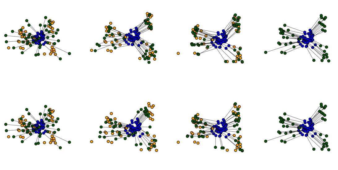
Figure 7: Assignments between two point clouds $\nu_{0}$ (in blue) and $\nu_{1}$ (in yellow) composed of $40$ points, for different values of $K$. Green points represent $T\#\nu_{0}$, where $T=T_{rand}$ on the first line and $T=T_{mean}$ on the second line. The four columns correspond respectively to $K=1,5,10,40$. Observe that for $K=1$, only one Gaussian is used for each set of points, and $T\#\nu_{0}$ is quite far from $\nu_{1}$ (in this case, $T_{rand}$ and $T_{mean}$ coincide). When $K$ increases, the discrete distribution $T\#\nu_{0}$ becomes closer to $\nu_{1}$, especially for $T=T_{rand}$. When $K$ is chosen equal to the number of points, we obtain the result of the $W_{2}$-optimal transport between $\nu_{0}$ and $\nu_{1}$.

7 Two applications in image processing

We have already illustrated the behaviour of the distance $MW_{2}$ in small dimension. In the following, we investigate more involved examples in larger dimension. In the last ten years, optimal transport has been thoroughly used for various applications in image processing and computer vision, including color transfer, texture synthesis, shape matching. We focus here on two simple applications: on the one hand, color transfer, that involves to transport mass in dimension $d=3$ since color histograms are 3D histograms, and on the other hand patch-based texture synthesis, that necessitates transport in dimension $p^{2}$ for $p\times p$ patches. These two applications require to compute transport plans or barycenters between potentially millions of points. We will see that the use of $MW_{2}$ makes these computations much easier and faster than the use of classical optimal transport, while yielding excellent visual results. The codes of the different experiments are available through Jupyter notebooks on https://github.com/judelo/gmmot.

7.1 Color transfer

We start with the problem of color transfer. A discrete color image can be seen as a function $u:\Omega\rightarrow\mathbb{R}^{3}$ where $\Omega=\{0,\dots n_{r}-1\}\times\{0,\dots n_{c}-1\}$ is a discrete grid. The image size is $n_{r}\times n_{c}$ and for each $i\in\Omega$, $u(i)\in\mathbb{R}^{3}$ is a set of three values corresponding to the intensities of red, green and blue in the color of the pixel. Given two images $u_{0}$ and $u_{1}$ on grids $\Omega_{0}$ and $\Omega_{1}$, we define the discrete color distributions $\eta_{k}=\frac{1}{|\Omega_{k}|}\sum_{i\in\Omega_{k}}\delta_{u_{k}(i)}$, $k=0,1$, and we approximate these two distributions by Gaussian mixtures $\mu_{0}$ and $\mu_{1}$ thanks to the Expectation-Maximization (EM) algorithm. Keeping the notations used previously in the paper, we write $K_{k}$ the number of Gaussian components in the mixture $\mu_{k}$, for $k=0,1$. We compute the $MW_{2}$ map between these two mixtures and the corresponding $T_{mean}$. We use it to compute $T_{mean}(u_{0})$, an image with the same content as $u_{0}$ but with colors much closer to those of $u_{1}$. Figure 8 illustrates this process on two paintings by Renoir and Gauguin, respectively Le déjeuner des canotiers and Manhana no atua. For this experiment, we choose $K_{0}=K_{1}=10$. The corresponding transport map for $MW_{2}$ is relatively fast to compute (less than one minute with a non-optimized Python implementation, using the POT library [15] for computing the map between the discrete distributions of $10$ masses). We also show on the same figure $T_{rand}(u_{0})$, the result of the sliced optimal transport [25, 5], and the result of the separable optimal transport (i.e. on each color channel separately). Notice that the complete optimal transport on such huge discrete distributions (approximately 800000 Dirac masses for these $1024\times 768$ images) is hardly tractable in practice. As could be expected, the image $T_{rand}(u_{0})$ is much noisier than the image $T_{mean}(u_{0})$. We show on Figure 9 the discrete color distributions of these different images and the corresponding classes provided by EM (each point is assigned to its most likely class).

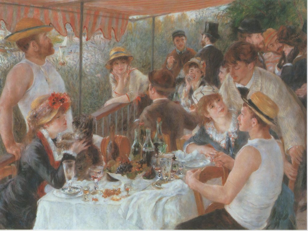
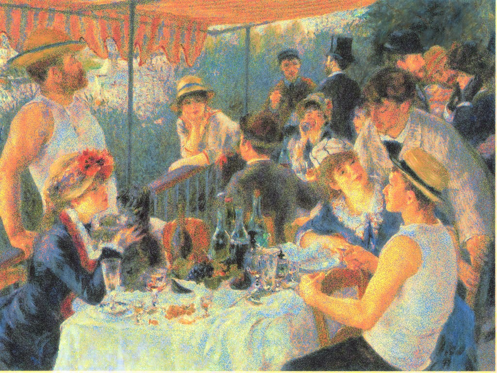
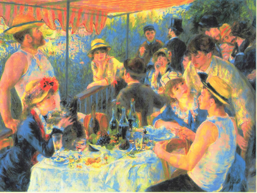
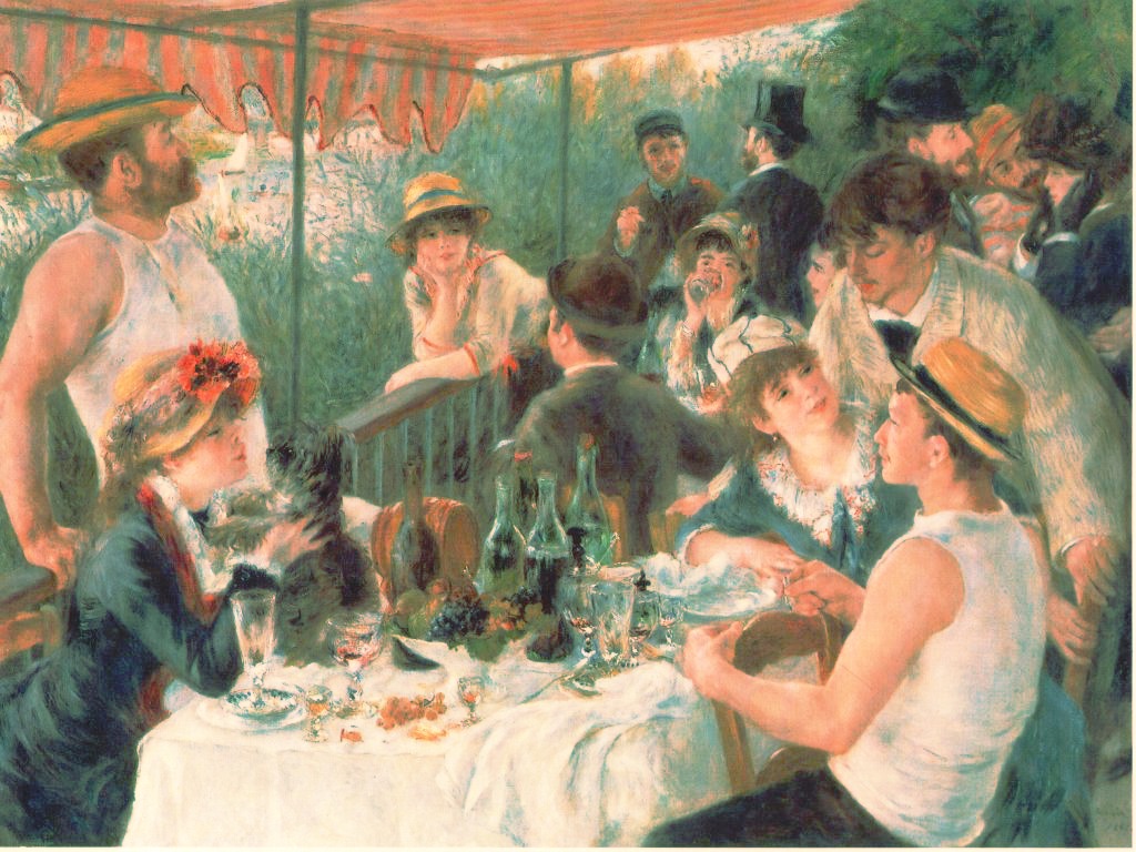
Figure 8: First line, images $u_{0}$ and $u_{1}$ (two paintings by Renoir and Gauguin). Second line, $T_{mean}(u_{0})$ and $T_{rand}(u_{0})$. Third line, color transfer with the sliced optimal transport [25, 5], that we denote by $SOT(u_{0})$ and result of the separable optimal transport (color transfer is applied separately on the three dimensions - channels - of the color distributions).

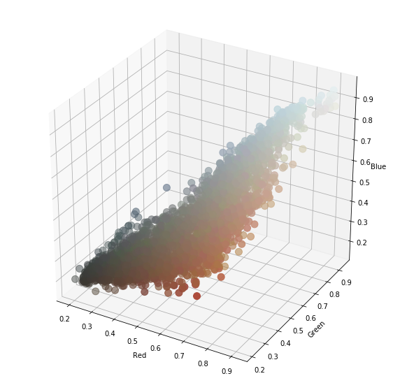
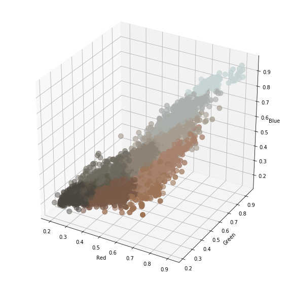
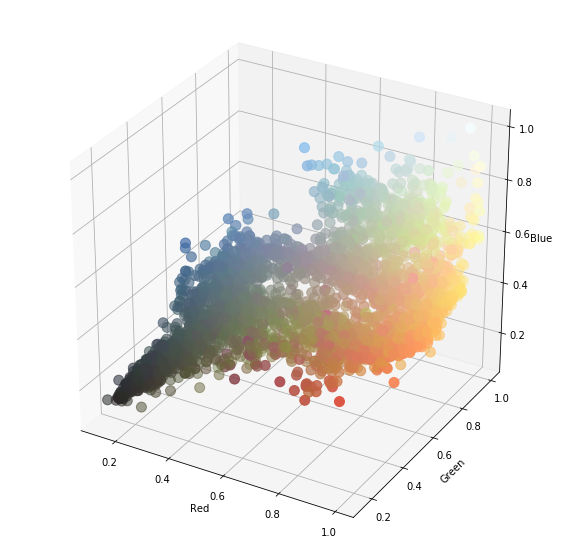
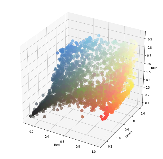
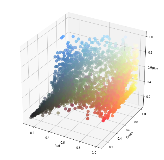
Figure 9: The images $u_{0}$ and $u_{1}$ are the ones of Figure 8. First line: color distribution of the image $u_{0}$, the $10$ classes found by the EM algorithm, and color distribution of $T_{mean}(u_{0})$. Second line: color distribution of the image $u_{1}$, the $10$ classes found by the EM algorithm, and color distribution of $T_{rand}(u_{0})$.

The value $K=10$ that we have chosen here is the result of a compromise. Indeed, when $K$ is too small, the approximation by the mixtures is generally too rough to represent the complexity of the color data properly. At the opposite, we have observed that increasing the number of components does not necessarily help since the corresponding transport map will loose regularity. For color transfer experiments, we found in practice that using around $10$ components yields the best results. We also illustrate this on Figure 10, where we show the results of the color transfer with $MW_{2}$ for different values of $K$. On the different images, one can appreciate how the color distribution gets closer and closer to the one of the target image as $K$ increases.

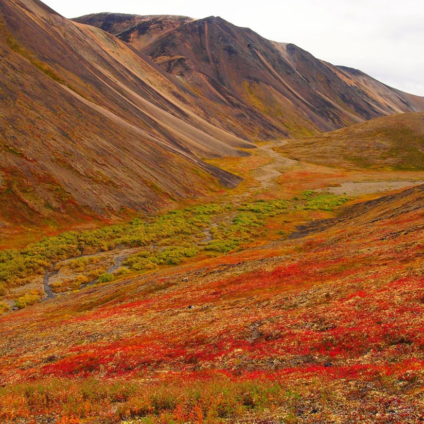
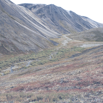
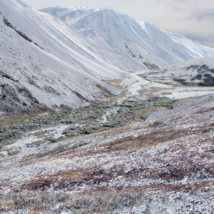
	$K=1$	$K=3$	$K=10$

Figure 10: The left-most image is the “red mountain” image, and its color distribution is modified to match the one of the right-most image (the “white mountain” image) with $MW_{2}$ using respectively $K=1$, $K=3$ and $K=10$ components in the Gaussian mixtures.

We end this section with a color manipulation experiment, shown on Figure 11. Four different images being given, we create barycenters for $MW_{2}$ between their four color palettes (represented again by mixtures of 10 Gaussian components), and we modify the first of the four images so that its color palette spans this space of barycenters. For this experiment (and this experiment only), a spatial regularization step is applied in post-processing [24] to remove some artifacts created by these color transformations between highly different images.

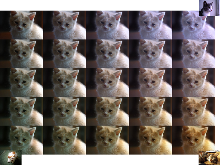
Figure 11: In this experiment, the top left image is modified in such a way that its color palette goes through the $MW_{2}$-barycenters between the color palettes of the four corner images. Each color palette is represented as a mixture of 10 Gaussian components. The weights used for the barycenters are bilinear with respect to the four corners of the rectangle.

7.2 Texture synthesis

Given an exemplar texture image $u:\Omega\rightarrow R^{3}$, the goal of texture synthesis is to synthetize images with the same perceptual characteristics as $u$, while keeping some innovative content. The literature on texture synthesis is rich, and we will only focus here on a bilevel approach proposed recently in [16]. The method relies on the optimal transport between a continuous (Gaussian or Gaussian mixtures) distribution and a discrete distribution (distribution of the patches of the exemplar texture image). The first step of the method can be described as follows. For a given exemplar image $u:\Omega\rightarrow R^{3}$, the authors compute the asymptotic discrete spot noise (ADSN) associated with $u$, which is the stationary Gaussian random field $U:\mathbb{Z}^{2}\rightarrow\mathbb{R}^{3}$ with same mean and covariance as $u$, i.e.

$$\forall x\in\mathbb{Z}^{2},\;U(x)=\bar{u}+\sum_{y\in\mathbb{Z}^{2}}t_{u}(y)W(x-y),\;\text{ where }\begin{cases}\bar{u}=\frac{1}{|\Omega|}\sum_{x\in\Omega}u(x)\\ t_{u}=\frac{1}{\sqrt{|\Omega|}}(u-\bar{u})\mathbf{1}_{\Omega},\end{cases}$$

with $W$ a standard normal Gaussian white noise on $\mathbb{Z}^{2}$. Once the ADSN $U$ is computed, they extract a set $S$ of $p\times p$ sub-images (also called patches) of $u$. In our experiments, we extract one patch for each pixel of $u$ (excluding the borders), so patches are overlapping and the number of patches is approximately equal to the image size. The authors of [16] then define $\eta_{1}$ the empirical distribution of this set of patches (thus $\eta_{1}$ is in dimension $3\times p\times p$, i.e. $27$ for $p=3$) and $\eta_{0}$ the Gaussian distribution of patches of $U$, and compute the semi-discrete optimal transport map $T_{SD}$ from $\eta_{0}$ to $\eta_{1}$. This map $T_{SD}$ is then applied to each patch of a realization of $U$, and an ouput synthetized image $v$ is obtained by averaging the transported patches at each pixel. Since the semi-discrete optimal transport step is numerically very expensive in such high dimension, we propose to make use of the $MW_{2}$ distance instead. For that, we approximate the two discrete patch distributions of $u$ and $U$ by Gaussian Mixture models $\mu_{0}$ and $\mu_{1}$, and we compute the optimal map $T_{mean}$ for $MW_{2}$ between them. The rest of the algorithm is similar to the one described in [16]. Figure 12 shows the results for different choices of exemplar images $u$. In practice, we use $K_{0}=K_{1}=10$, as in color transfer, and $3\times 3$ color patches. The results obtained with our approach are visually very similar to the ones obtained with [16], for a computational time approximately 10 times smaller. More precisely, for instance for an image of size $256\times 256$, the proposed approach takes about $35$ seconds, whereas the semi-discrete approach of [16] takes about $400$ seconds. We are currently exploring a multiscale version of this approach, inspired by the recent [22].

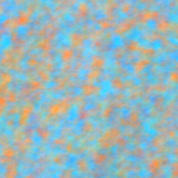
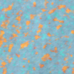
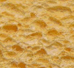
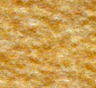
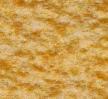
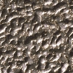
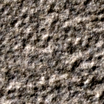
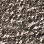
Figure 12: Left, original texture $u$. Middle, ADSN $U$. Right, synthetized version.

8 Discussion and conclusion

In this paper, we have defined a Wasserstein-type distance on the set of Gaussian mixture models, by restricting the set of possible coupling measures to Gaussian mixtures. We have shown that this distance, with an explicit discrete formulation, is easy to compute and suitable to compute transport plans or barycenters in high dimensional problems where the classical Wasserstein distance remains difficult to handle. We have also discussed the fact that the distance $MW_{2}$ could be extended to other types of mixtures, as soon as we have a marginal consistency property and an identifiability property similar to the one used in the proof of Proposition 4. In practice, Gaussian mixture models are versatile enough to represent large classes of concrete and applied problems. One important question raised by the introduced framework and its generalization in Section 6.2 is how to estimate the mixtures for discrete data, since the obtained result will depend on the number $K$ of Gaussian components in the mixtures and on the parameter $\lambda$ that weights the data-fidelity terms. If the number of Gaussian components is chosen large enough, and covariances small enough, the transport plan for $MW_{2}$ will look very similar to the one of $W_{2}$, but at the price of a high computational cost. If, on the contrary, we choose a very small number of components (like in the color transfer experiments of Section 7.1), the resulting optimal transport map will be much simpler, which seems to be desirable for some applications.

Appendix: proofs

Density of $GMM_{d}(\infty)$ in $\mathcal{P}_{p}(\mathbb{R}^{d})$

Lemma (Lemma 3.1).

The set

$$\left\{\sum_{k=1}^{N}\pi_{k}\delta_{y_{k}}\;;\;N\in\mathbb{N},\;(y_{k})_{k}\in(\mathbb{R}^{d})^{N},\;(\pi_{k})_{k}\in\Gamma_{N}\right\}$$

is dense in $\mathcal{P}_{p}(\mathbb{R}^{d})$ for the metric $W_{p}$, for any $p\geq 1$.

Proof 8.1.

The proof is adapted from the proof of Theorem 6.18 in [31] and given here for the sake of completeness.

Let $\mu\in\mathcal{P}_{p}(\mathbb{R}^{d})$. For each $\epsilon>0$, we can find $r$ such that $\int_{B(0,r)^{c}}\|y\|^{p}d\mu(x)\leq\epsilon^{p}$, where $B(0,r)\subset\mathbb{R}^{d}$ is the ball of center $0$ and radius $r$, and $B(0,r)^{c}$ denotes its complementary set in $\mathbb{R}^{d}$. The ball $B(0,r)$ can be covered by a finite number of balls $B(y_{k},\epsilon)$, $1\leq k\leq N$. Now, define $B_{k}=B(y_{k},\epsilon)\setminus\cup_{1\leq j<k}B(y_{j},\epsilon)$, all these sets are disjoint and still cover $B(0,r)$.
Define $\phi:\mathbb{R}^{d}\rightarrow\mathbb{R}^{d}$ on $\mathbb{R}^{d}$ such that

$$\forall k,\;\forall y\in B_{k}\cap B(0,r),\,\,\phi(y)=y_{k}\;\text{ and }\;\forall y\in B(0,r)^{c},\,\,\phi(y)=0.$$

Then,

$$\phi\#\mu=\sum_{k=1}^{N}\mu(B_{k}\cap B(0,r))\delta_{y_{k}}+\mu(B(0,r)^{c})\delta_{0}$$

and

$$W_{p}^{p}(\phi\#\mu,\mu) \leq \int_{\mathbb{R}^{d}}\|y-\phi(y)\|^{p}d\mu(y)$$

$$\leq \epsilon^{p}\int_{B(0,r)}d\mu(y)+\int_{B(0,r)^{c}}\|y\|^{p}d\mu(y)\leq\epsilon^{p}+\epsilon^{p}=2\epsilon^{p},$$

which finishes the proof.

Identifiability properties of Gaussian mixture models

Proposition (Proposition 2).

The set of finite Gaussian mixtures is identifiable, in the sense that two mixtures $\mu_{0}=\sum_{k=1}^{K_{0}}\pi_{0}^{k}\mu_{0}^{k}$ and $\mu_{1}=\sum_{k=1}^{K_{1}}\pi_{1}^{k}\mu_{1}^{k}$, written such that all $\{\mu_{0}^{k}\}_{k}$ (resp. all $\{\mu_{1}^{j}\}_{j}$) are pairwise distinct, are equal if and only if $K_{0}=K_{1}$ and we can reorder the indexes such that for all $k$, $\pi_{0}^{k}=\pi_{1}^{k}$, $m_{0}^{k}=m_{1}^{k}$ and $\Sigma_{0}^{k}=\Sigma_{1}^{k}$.

This result is classical and the proof is also given here in the Appendix for the sake of completeness.

Proof 8.2.

This proof is an adaptation and simplification of the proof of Proposition 2 in [34]. First, assume that $d=1$ and that two Gaussian mixtures are equal:

(28) $$\sum_{k=1}^{K_{0}}\pi_{0}^{k}\mu_{0}^{k}=\sum_{j=1}^{K_{1}}\pi_{1}^{j}\mu_{1}^{j}.$$

We start by identifying the Dirac masses from both sums, so only non-degenerate Gaussian components remain. Writing $\mu_{i}^{k}=\mathcal{N}(m_{i}^{k},(\sigma_{i}^{k})^{2})$, it follows that

$$\sum_{k=1}^{K_{0}}\frac{\pi_{0}^{k}}{\sigma_{0}^{k}}e^{-\frac{(x-m_{0}^{k})^{2}}{2(\sigma_{0}^{k})^{2}}}=\sum_{j=1}^{K_{1}}\frac{\pi_{1}^{j}}{\sigma_{1}^{j}}e^{-\frac{(x-m_{1}^{j})^{2}}{2(\sigma_{1}^{j})^{2}}},\;\;\forall x\in\mathbb{R}.$$

Now, define $k_{0}=\mathrm{argmax}_{k}\sigma_{0}^{k}$ and $j_{0}=\mathrm{argmax}_{j}\sigma_{1}^{j}$. If the maximum is attained for several values of $k$ (resp. $j$), we keep the one with the largest mean $m_{0}^{k}$ (resp. $m_{1}^{j}$). Then, when $x\rightarrow+\infty$, we have the equivalences

$$\sum_{k=1}^{K_{0}}\frac{\pi_{0}^{k}}{\sigma_{0}^{k}}e^{-\frac{(x-m_{0}^{k})^{2}}{2(\sigma_{0}^{k})^{2}}}\underset{x\to+\infty}{\sim}\frac{\pi_{0}^{k_{0}}}{\sigma_{0}^{k_{0}}}e^{-\frac{(x-m_{0}^{k_{0}})^{2}}{2(\sigma_{0}^{k_{0}})^{2}}}\;\;\text{ and }\sum_{j=1}^{K_{1}}\frac{\pi_{1}^{j}}{\sigma_{1}^{j}}e^{-\frac{(x-m_{1}^{j})^{2}}{2(\sigma_{1}^{j})^{2}}}\underset{x\to+\infty}{\sim}\frac{\pi_{1}^{j_{0}}}{\sigma_{1}^{j_{0}}}e^{-\frac{(x-m_{1}^{j_{0}})^{2}}{2(\sigma_{1}^{j_{0}})^{2}}}.$$

Since the two sums are equal, these two terms must also be equivalent when $x\rightarrow+\infty$, which implies necessarily that $\sigma_{0}^{k_{0}}=\sigma_{1}^{j_{0}}$, $m_{0}^{k_{0}}=m_{1}^{j_{0}}$ and $\pi_{0}^{k_{0}}=\pi_{1}^{j_{0}}$. Now, we can remove these two components from the two sums and we obtain

$$\sum_{k=1\dots K_{0},\;k\neq k_{0}}\frac{\pi_{0}^{k}}{\sigma_{0}^{k}}e^{-\frac{(x-m_{0}^{k})^{2}}{2(\sigma_{0}^{k})^{2}}}=\sum_{j=1\dots K_{1},\;j\neq j_{0}}\frac{\pi_{1}^{j}}{\sigma_{1}^{j}}e^{-\frac{(x-m_{1}^{j})^{2}}{2(\sigma_{1}^{j})^{2}}},\;\;\;\forall x\in\mathbb{R}.$$

We can start over and show recursively that all components are equal.

For $d>1$, assume once again that two Gaussian mixtures $\mu_{0}$ and $\mu_{1}$ are equal, written as in Equation (28). The projection of this equality yields

(29) $$\sum_{k=1}^{K_{0}}\pi_{0}^{k}\mathcal{N}(\langle m_{0}^{k},\xi\rangle,\xi^{t}\Sigma_{0}^{k}\xi)=\sum_{j=1}^{K_{1}}\pi_{1}^{j}\mathcal{N}(\langle m_{1}^{j},\xi\rangle,\xi^{t}\Sigma_{1}^{j}\xi),\;\;\;\forall\xi\in\mathbb{R}^{d}.$$

At this point, observe that for some values of $\xi$, some of these projected components may not be pairwise distinct anymore, so we cannot directly apply the result for $d=1$ to such mixtures. However, since the pairs $(m_{0}^{k},\Sigma_{0}^{k})$ (resp. $(m_{1}^{j},\Sigma_{1}^{j})$) are all distinct, then for $i=0,1$, the set

$$\Theta_{i}=\bigcup_{1\leq k,k^{\prime}\leq K_{i}}\left\{\xi\;\;\text{s.t.}\;\langle m_{i}^{k}-m_{i}^{k^{\prime}},\xi\rangle=0\;\;\text{and}\;\;\xi^{t}\left(\Sigma_{i}^{k}-\Sigma_{i}^{k^{\prime}}\right)\xi=0\right\}$$

is of Lebesgue measure $0$ in $\mathbb{R}^{d}$. For any $\xi$ in $\mathbb{R}^{d}\setminus\Theta_{0}\cup\Theta_{1}$, the pairs $\{(\langle m_{0}^{k},\xi\rangle,\xi^{t}\Sigma_{0}^{k}\xi)\}_{k}$ (resp. $\{(\langle m_{1}^{j},\xi\rangle,\xi^{t}\Sigma_{1}^{j}\xi)\}_{j}$) are pairwise distinct. Consequently, using the first part of the proof (for $d=1$), we can deduce that $K_{0}=K_{1}$ and that

(30) $$\mathbb{R}^{d}\setminus\Theta_{0}\cup\Theta_{1}\subset\bigcap_{k}\bigcup_{j}\Xi_{k,j}$$

where

$$\Xi_{k,j}=\left\{\xi,\;\;\text{s.t.}\;\pi_{0}^{k}=\pi_{1}^{j},\;\;\langle m_{0}^{k}-m_{1}^{j},\xi\rangle=0\;\;\text{and}\;\;\xi^{t}\left(\Sigma_{0}^{k}-\Sigma_{1}^{j}\right)\xi=0\right\}.$$

Now, assume that the two sets $\{(\pi_{0}^{k},m_{0}^{k},\Sigma_{0}^{k})\}_{k}$ and $\{(\pi_{1}^{j},m_{1}^{j},\Sigma_{1}^{j})\}_{j}$ are different. Since each of these sets is composed of different triplets, it is equivalent to assume that there exists $k$ in $\{1,\dots K_{0}\}$ such that $(\pi_{0}^{k},m_{0}^{k},\Sigma_{0}^{k})$ is different from all triplets $(\pi_{1}^{j},m_{1}^{j},\Sigma_{1}^{j})$. In this case, the sets $\Xi_{k,j}$ for $j=1,\dots K_{0}$ are all of Lebesgue measure $0$ in $\mathbb{R}^{d}$, which contradicts (30). We conclude that the sets $\{(\pi_{0}^{k},m_{0}^{k},\Sigma_{0}^{k})\}_{k}$ and $\{(\pi_{1}^{j},m_{1}^{j},\Sigma_{1}^{j})\}_{j}$ are equal.

References

- [1] M. Agueh and G. Carlier, Barycenters in the Wasserstein space, SIAM Journal on Mathematical Analysis, 43 (2011), pp. 904–924.
- [2] P. C. Álvarez-Esteban, E. del Barrio, J. Cuesta-Albertos, and C. Matrán, A fixed-point approach to barycenters in Wasserstein space, Journal of Mathematical Analysis and Applications, 441 (2016), pp. 744–762.
- [3] J. Bion–Nadal and D. Talay, On a Wasserstein-type distance between solutions to stochastic differential equations, Ann. Appl. Probab., 29 (2019), pp. 1609–1639, https://doi.org/10.1214/18-AAP1423.
- [4] C. M. Bishop, Pattern recognition and machine learning, springer, 2006.
- [5] N. Bonneel, J. Rabin, G. Peyré, and H. Pfister, Sliced and Radon Wasserstein barycenters of measures, Journal of Mathematical Imaging and Vision, 51 (2015), pp. 22–45.
- [6] Y. Chen, T. T. Georgiou, and A. Tannenbaum, Optimal transport for Gaussian mixture models, arXiv preprint arXiv:1710.07876, (2017).
- [7] Y. Chen, T. T. Georgiou, and A. Tannenbaum, Optimal Transport for Gaussian Mixture Models, IEEE Access, 7 (2019), pp. 6269–6278, https://doi.org/10.1109/ACCESS.2018.2889838.
- [8] Y. Chen, J. Ye, and J. Li, A distance for HMMS based on aggregated Wasserstein metric and state registration, in European Conference on Computer Vision, Springer, 2016, pp. 451–466.
- [9] Y. Chen, J. Ye, and J. Li, Aggregated Wasserstein Distance and State Registration for Hidden Markov Models, IEEE Transactions on Pattern Analysis and Machine Intelligence, (2019), https://doi.org/10.1109/TPAMI.2019.2908635.
- [10] L. Chizat, G. Peyré, B. Schmitzer, and F.-X. Vialard, Scaling algorithms for unbalanced optimal transport problems, Mathematics of Computation, 87 (2017), pp. 2563–2609.
- [11] C.-A. Deledalle, S. Parameswaran, and T. Q. Nguyen, Image denoising with generalized Gaussian mixture model patch priors, SIAM Journal on Imaging Sciences, 11 (2019), pp. 2568–2609.
- [12] J. Delon and A. Houdard, Gaussian priors for image denoising, in Denoising of Photographic Images and Video, Springer, 2018, pp. 125–149.
- [13] A. P. Dempster, N. M. Laird, and D. B. Rubin, Maximum likelihood from incomplete data via the EM algorithm, Journal of the Royal Statistical Society: Series B (Methodological), 39 (1977), pp. 1–22.
- [14] D. Dowson and B. Landau, The Fréchet distance between multivariate normal distributions, Journal of multivariate analysis, 12 (1982), pp. 450–455.
- [15] R. Flamary and N. Courty, POT Python Optimal Transport library, 2017, https://github.com/rflamary/POT.
- [16] B. Galerne, A. Leclaire, and J. Rabin, Semi-discrete optimal transport in patch space for enriching Gaussian textures, in International Conference on Geometric Science of Information, Springer, 2017, pp. 100–108.
- [17] W. Gangbo and A. Świkech, Optimal maps for the multidimensional Monge-Kantorovich problem, Communications on Pure and Applied Mathematics: A Journal Issued by the Courant Institute of Mathematical Sciences, 51 (1998), pp. 23–45.
- [18] M. Gelbrich, On a formula for the l2 wasserstein metric between measures on euclidean and hilbert spaces, Mathematische Nachrichten, 147 (1990), pp. 185–203.
- [19] A. Houdard, C. Bouveyron, and J. Delon, High-dimensional mixture models for unsupervised image denoising (HDMI), SIAM Journal on Imaging Sciences, 11 (2018), pp. 2815–2846.
- [20] O. Kallenberg, Foundations of modern probability, Probability and its Applications (New York), Springer-Verlag, New York, second ed., 2002.
- [21] Y. Kanoh, Consistency property of elliptical probability density functions, Journal of Multivariate Analysis, 51 (1994), pp. 139–147.
- [22] A. Leclaire and J. Rabin, A multi-layer approach to semi-discrete optimal transport with applications to texture synthesis and style transfer, preprint hal-02331068, (2019).
- [23] G. Peyré and M. Cuturi, Computational optimal transport, Foundations and Trends® in Machine Learning, 11 (2019), pp. 355–607.
- [24] J. Rabin, J. Delon, and Y. Gousseau, Removing artefacts from color and contrast modifications, IEEE Transactions on Image Processing, 20 (2011), pp. 3073–3085.
- [25] J. Rabin, G. Peyré, J. Delon, and M. Bernot, Wasserstein barycenter and its application to texture mixing, in International Conference on Scale Space and Variational Methods in Computer Vision, Springer, 2011, pp. 435–446.
- [26] L. Rüschendorf and L. Uckelmann, On the n-coupling problem, Journal of multivariate analysis, 81 (2002), pp. 242–258.
- [27] F. Santambrogio, Optimal Transport for Applied Mathematicians, Birkäuser, Basel, 2015.
- [28] A. M. Teodoro, M. S. Almeida, and M. A. Figueiredo, Single-frame Image Denoising and Inpainting Using Gaussian Mixtures, in ICPRAM (2), 2015, pp. 283–288.
- [29] A. Van Den Oord and B. Schrauwen, The student-t mixture as a natural image patch prior with application to image compression, The Journal of Machine Learning Research, 15 (2014), pp. 2061–2086.
- [30] C. Villani, Topics in Optimal Transportation Theory, vol. 58 of Graduate Studies in Mathematics, American Mathematical Society, 2003.
- [31] C. Villani, Optimal transport: old and new, vol. 338, Springer Science & Business Media, 2008.
- [32] Y.-Q. Wang and J.-M. Morel, SURE Guided Gaussian Mixture Image Denoising, SIAM Journal on Imaging Sciences, 6 (2013), pp. 999–1034, https://doi.org/10.1137/120901131.
- [33] G.-S. Xia, S. Ferradans, G. Peyré, and J.-F. Aujol, Synthesizing and mixing stationary Gaussian texture models, SIAM Journal on Imaging Sciences, 7 (2014), pp. 476–508.
- [34] S. J. Yakowitz and J. D. Spragins, On the identifiability of finite mixtures, Ann. Math. Statist., 39 (1968), pp. 209–214, https://doi.org/10.1214/aoms/1177698520.
- [35] G. Yu, G. Sapiro, and S. Mallat, Solving inverse problems with piecewise linear estimators: from Gaussian mixture models to structured sparsity, IEEE Trans. Image Process., 21 (2012), pp. 2481–99, https://doi.org/10.1109/TIP.2011.2176743.
- [36] D. Zoran and Y. Weiss, From learning models of natural image patches to whole image restoration, in 2011 Int. Conf. Comput. Vis., IEEE, Nov. 2011, pp. 479–486, https://doi.org/10.1109/ICCV.2011.6126278.