Dissecting the growth of the power spectrum for primordial black holes

Abstract

We consider the steepest rate at which the power spectrum from single field inflation can grow, with the aim of providing a simple explanation for the $k^{4}$ growth found recently. With this explanation in hand we show that a slightly steeper $k^{5}(\log k)^{2}$ growth is in fact possible. Moreover, we argue that the power spectrum after a steep growth cannot immediately decay, but must remain large for the $k$ modes which exit during a $\sim 2$ e-fold period. We also briefly consider how a strong growth can affect the spectral index of longer wavelengths preceding the growth, and show that even the conversion of isocurvature modes likely cannot lead to a stronger growth. These results have implications for the formation of primordial black holes, and other phenomena which require a large amplitude of power spectrum at short scales.

I Introduction

How steeply can ${\cal P}_{\cal R}$, the power spectrum of the primordial curvature perturbation, grow with scale? This interesting question is addressed in the recent paper of Byrnes et al. Byrnes et al. (2019). If produced during inflation, one might think that the classic relation, ${\cal P}_{\cal R}\sim{H_{*}^{2}}/{\epsilon_{*}}$, implies that a model with a sudden change in $\epsilon$ to a much smaller value would allow an arbitrarily steep growth, through for example the rapid flattening of the inflationary potential. Here $H_{*}$ is the Hubble rate at which a given scale is equal to the cosmological horizon during inflation, and $\epsilon_{*}$ is the value of slow-roll parameter $\epsilon=-\dot{H}/H^{2}$ at that time. However, the slow-roll solution to the equations of motion that the above relation for ${\cal P}_{\cal R}$ relies on becomes invalid for a period around such a flattening. Byrnes et al.Byrnes et al. (2019) therefore explored analytic solutions to the evolution of perturbations in models with $\epsilon\ll 1$ (so inflation always proceeds), but with the second slow-roll parameter, $\eta=\dot{\epsilon}/(H\epsilon)$, taking a series of discrete values between $0$ and large negative values, matching the perturbations and their first derivative at each change in $\eta$. This setup encompasses, but is more general than, the case of a rapid flattening of the inflationary potential described above. Doing so, the steepest sustained growth that they observed was in fact proportional to $k^{4}$, which they then argued is the steepest possible. Numerical simulations backed up their conclusion.

This result is of considerable interest. The discovery by LIGO of binary in-spiralling black holes with masses of the order of a few $M_{\odot}$ Abbott et al. (2016); Abbott et al. (2018a, b), as well as the continued absence of a microphysical explanation for dark matter, have lead to a renewed interest in primordial black holes (PBHs) Carr and Hawking (1974); Bird et al. (2016); Sasaki et al. (2016); Carr et al. (2016, 2017). If PBHs form in the radiation era which follows inflation, however, ${\cal P}_{\cal R}$ must grow by at least seven orders of magnitude between the scales which account for the formation of large scale structure in the universe and the scales which lead to PBHs Zaballa et al. (2007); Josan et al. (2009); Cole and Byrnes (2018); Germani and Prokopec (2017); Germani and Musco (2019). Moreover, if PBHs are to form only in specific mass ranges to evade constraints Carr et al. (2010, 2017); Byrnes et al. (2019), the particular form of the growth and decay of the power spectrum is very important. The result of Ref. Byrnes et al. (2019) is also of interest more generally, for example a large power spectrum at short scales can produce gravitational waves at second order in perturbation theory Ananda et al. (2007); Baumann et al. (2007); Alabidi et al. (2012); Di and Gong (2018); Kohri and Terada (2018); Clesse et al. (2018).

In this short paper we build on the work of Byrnes et al. Byrnes et al. (2019) by studying the same system. Our aim is to provide a clear and simple explanation of where the $k^{4}$ growth comes from, and with this explanation in hand to ask whether $k^{4}$ growth really is the steepest sustained growth in $k$ space that is possible. We show that this is in fact not the case, and that it is possible to have a steeper sustained growth proportional to $k^{5}(\log k)^{2}$ in single field inflation. We also consider how the spectrum preceding the growth is affected by the behaviour needed to produce a strong growth, and comment on the subsequent rate of decay which cannot be instantaneous. Finally we apply the insight we develop to the isocurvature sector to see if it could in principle be responsible for an even steeper growth of ${\cal P}_{\cal R}$ – we find this is likely not possible.

II slow-roll to ultra-slow-roll

Let us follow Byrnes et al. Byrnes et al. (2019), and others Germani and Prokopec (2017); Ballesteros and Taoso (2018); Di and Gong (2018); Cheng et al. (2019); Bhaumik and Jain (2019), and study first the most natural situation which leads to a steep growth in the power spectrum. Consider canonical single-field inflation with a potential $V(\phi)$ with small gradient $V^{\prime}_{1}$ with $V^{\prime}_{1}\ll V$, followed by a sudden transition to gradient $V^{\prime}_{2}\ll V^{\prime}_{1}$, as illustrated in Fig. (1a). Fourier modes of the comoving curvature perturbation ${\cal R}$ which are able to transition between their vacuum state and their asymptotic form, in which they are constant, while slow-roll inflation occurs on the $V^{\prime}_{1}$ region have a close to scale-invariant spectrum: ${\cal P}_{\cal R}(k)\sim{V^{4}}/{V^{\prime}_{1}}^{2}$, while modes which can move from vacuum to asymptotic form on the $V^{\prime}_{2}$ region have spectrum ${\cal P}_{\cal R}(k)\sim{V^{4}}/{V^{\prime}_{2}}^{2}$. The velocity of the inflaton field, ${\rm d}\phi/{\rm d}N$, for the slow roll attractor solution in the two regimes is $-V^{\prime}_{1}/V$ and $-V^{\prime}_{2}/V$, respectively ($N\equiv\log a$ is the number of e-folds, $a$ the scale factor). This implies that at the transition the velocity is initially much higher than the second slow-roll value, and must decay to reach it. Initially the gradient of the potential is irrelevant, and the steepest that this can happen is at the rate for a free field of ${\rm d}\phi/{\rm d}N\propto a^{-3}$, where we assume the Hubble rate is approximately constant. This represents a phase of ultra-slow-roll (USR) inflation, followed by slow-roll inflation again at the new lower velocity, as can be seen in Fig. (1b). This behaviour leads to an approximately scale-invariant spectrum for modes which exit sufficiently early in the first slow-roll phase followed by a spectrum which grows in proportion to $k^{4}$, and finally a near scale-invariant spectrum again, as seen in Figs. (1c) and (1d) where we indicate the phases during which perturbations exit the horizon. We have generated these figures using the open source code PyTransport Dias et al. (2016); Mulryne and Ronayne (2016); Ronayne and Mulryne (2018) (see also Dias et al. (2016); Seery (2016); Butchers and Seery (2018) for a related package).

The question at hand now is what is the origin of the $k^{4}$ dependence. As we can see from Fig. (1) modes with the $k^{4}$ dependence exit during slow-roll inflation. We therefore consider the Sasaki-Mukhanov equation

$$v^{\prime\prime}_{k}+\left(k^{2}-\frac{z^{\prime\prime}}{z}\right)v_{k}=0\,,$$ (1)

where a dash indicates differentiation with respect to conformal time, $\tau$, and where

$$z^{2}=2a^{2}m_{\rm pl}^{2}\epsilon\,,$$ (2)

and

$$\frac{z^{\prime\prime}}{z}=(aH^{2})\left(2-\epsilon+\frac{3}{2}\eta+\frac{1}{4}\eta^{2}-\frac{1}{2}\epsilon\eta+\frac{1}{2}\frac{\dot{\eta}}{H}\right)\,,$$ (3)

where a dot indicates differentiation with respect to coordinate time. Recall also that $aH=-1/\tau$, and that $v$ is related to ${\cal R}$ through ${\cal R}=v/z$. Assuming $\epsilon\ll 1$ and defining

$$\nu^{2}=\frac{9}{4}+\frac{3}{2}\eta+\frac{1}{4}\eta^{2}+\frac{\dot{\eta}}{2H}\,,$$ (4)

one finds that for constant $\nu$ Eq. (1) has the general solution

$$v_{k}=\tilde{A}\sqrt{-\tau}H_{\nu}^{(1)}(-k\tau)+\tilde{B}\sqrt{-\tau}H_{\nu}^{(2)}(-k\tau)\,.$$ (5)

Note that for constant $\eta$, $\epsilon\propto(-\tau)^{-\eta}$. For modes which begin in the Bunch-Davies vacuum the solution is then normalised by fixing the constants $\tilde{A}$ and $\tilde{B}$ such that

$$v_{k}=\frac{\sqrt{\pi}}{2}e^{i\frac{\pi}{2}\left(\nu+\frac{1}{2}\right)}\sqrt{-\tau}H_{\nu}^{(1)}(-k\tau)\,.$$ (6)

Expanding in the super-horizon limit, $k\tau\to 0$, one finds

$$v_{k} \approx \frac{\sqrt{\pi}}{2}e^{i\frac{\pi}{2}\left(\nu+\frac{1}{2}\right)}\sqrt{-\tau}\left(-2^{\nu}i\frac{\Gamma(\nu)}{\pi}(-k\tau)^{-\nu}\right.$$ (7)

$$-2^{-2+\nu}i\frac{\Gamma(\nu)}{\pi(-1+\nu)}(-k\tau)^{-\nu+2}$$

$$\left.2^{-\nu}\frac{1+i\cot(\pi\nu)}{\Gamma(2+\nu)}(-k\tau)^{\nu}+\dots\right)\,,$$

where we have assumed $\nu$ is positive, but that $\nu\neq 1$. For ${\cal R}$ this implies

$${\cal R}_{k} \approx A\,(-\tau)^{-\nu+\frac{3}{2}+\frac{\eta}{2}}k^{-\nu}+B\,(-\tau)^{-\nu+\frac{7}{2}+\frac{\eta}{2}}k^{-\nu+2}$$ (8)

$$+ C\,(-\tau)^{\nu+\frac{3}{2}+\frac{\eta}{2}}k^{\nu}\,,$$

where in this equation we note that $A$, $B$ and $C$ are constants that are not free but take fixed values. Here we have retained three terms because it is not clear which of the last terms is the sub-leading term for a general $\nu$. Finally considering modes which exit during slow-roll inflation, one has $\eta\to 0$, $\nu\to 3/2$, and in this case one finds to sub-leading order that

$${\cal R}_{k}\approx Ak^{-3/2}+B(-\tau)^{2}k^{1/2}\,.$$ (9)

Given that ${\cal P}_{\cal R}(k)\sim k^{3}|{\cal R}|^{2}$, one can see that if the leading (constant) term dominates (as is usually expected), ${\cal P}_{\cal R}\propto k^{0}$, while if the sub-leading term would dominate the resulting scale-dependence would be ${\cal P}_{\cal R}\propto k^{4}$.

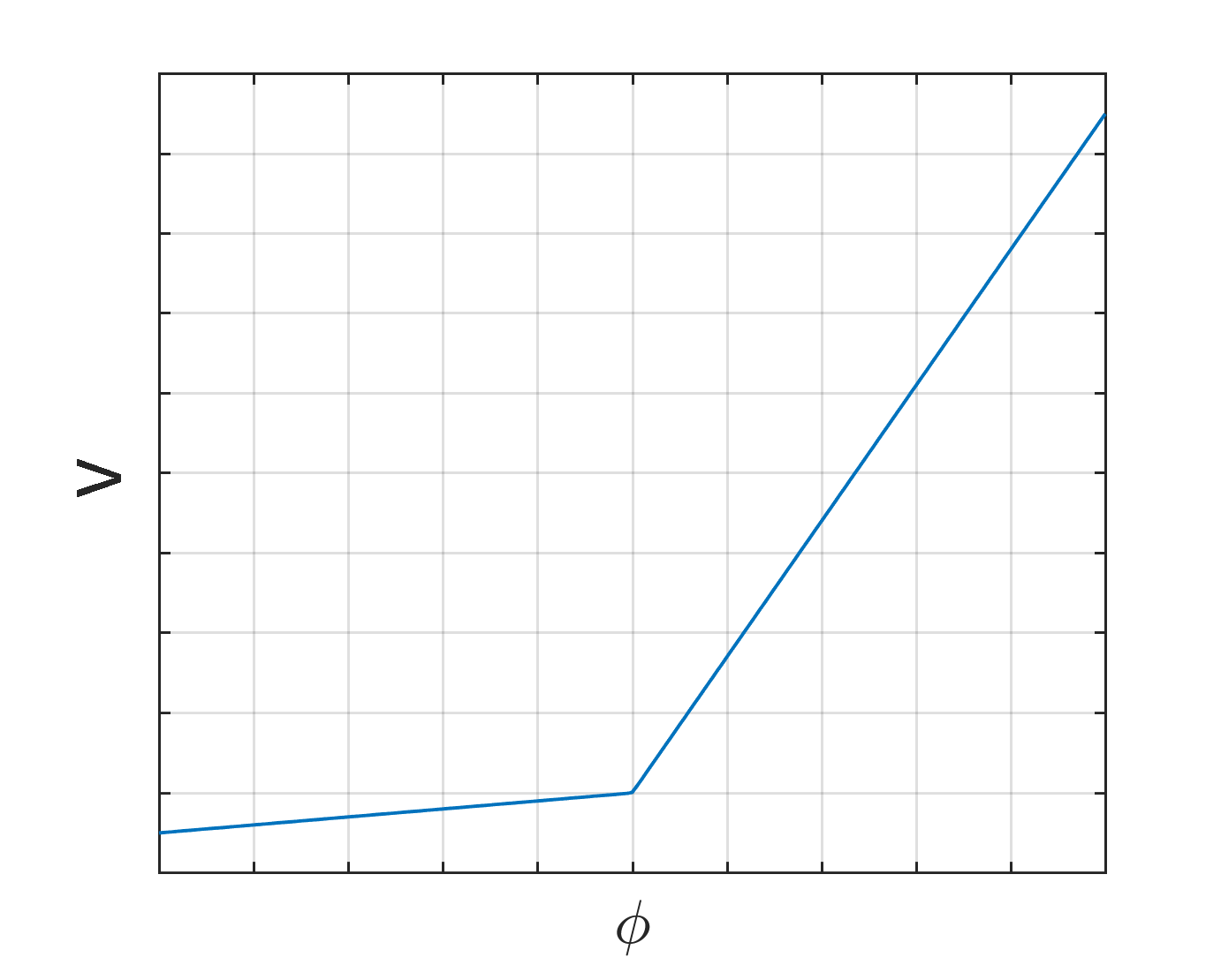
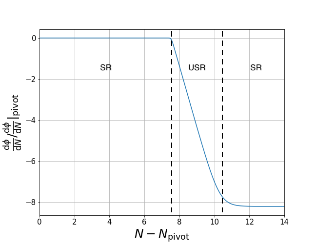
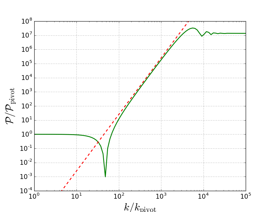
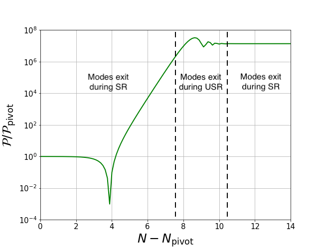
Figure 1: a (top left) shows schematically a potential that rapidly flattens; b (top right) shows the rate the field changes as it rolls along this potential, the $a^{-3}$ scaling can clearly been seen; c (bottom left) shows the resultant power spectrum against $k$, with $k^{4}$ dependence indicated by the dashed line; and d (bottom right) shows the power spectrum against exit time in e-folds, highlighting the regime in which different modes exit.

II.1 Matching

Now let us consider what happens if there is a transition to the USR phase. For this phase $\nu=-3/2$ and $\eta=-6$ and on scales larger than the horizon the general solution (5) gives

$${\cal R}_{k}=A_{2}(-\tau)^{-3}+B_{2}\dots\,,$$ (10)

where the subscript $2$ indicates quantities after the transition, and where we have only kept the leading term and sub-leading terms with independent coefficients $A_{2}$ and $B_{2}$. Note that one of the independent solutions to Eq. (1) for any $\nu$ will always lead to a constant ${\cal R}$ on super-horizon scales. To understand the fate of modes which exited during slow-roll inflation we now match solution (9) to (10). Matching both the solution and its first derivative, as required by the Israel junction conditions Israel (1966); Deruelle and Mukhanov (1995), at the time $\tau=-1$ (which is an arbitrary but convenient choice) we find

$$Ak^{-3/2} \approx A_{2}+B_{2}\,,$$ (11)

$$2Bk^{1/2} \approx -3A_{2}\,,$$ (12)

and hence $A_{2}\approx-2/3Bk^{1/2}$, $B_{2}\approx Ak^{-3/2}$, and

$${\cal R}_{k}=-2/3Bk^{1/2}(-\tau)^{-3}+Ak^{-3/2}+\dots\,.$$ (13)

Moreover, recall that $A$ and $B$ are fixed by the Bunch-Davies origin of the modes, and one can verify that $A\sim B$. Since we are considering modes with $k\ll 1$, at the matching time the second term in Eq. (13), which would lead to a scale-invariant spectrum, is initially the dominant one. However the second term, which has inherited the scale dependence of the decaying mode before the transition, is growing. For a given mode, therefore, if USR lasts sufficiently long this term will become dominant. If this happens for a range of scales, the spectrum for these modes gains a $k^{4}$ dependence, explaining the origin of this dependence. As was also discussed by Byrnes et al.Byrnes et al. (2019), the duration of the USR phase therefore plays a crucial role. The ratio of the power spectrum before and after the steep growth, $P_{{\cal R}\,\text{ratio}}$, is approximately given by the square of the ratio of the two terms in Eq. (13). Defining $\tau_{\text{USR}}=\tau_{\text{USR\,start}}/\tau_{\text{USR\,end}}$, therefore, we see that $P_{{\cal R}\,\text{ratio}}\approx\tau_{\text{USR}}^{6}$. For $P_{{\cal R}\,\text{ratio}}=10^{7}$, needed for PBH formation, then implies USR must last $\log 10^{7/6}\approx 2.7$ e-folds. Equation (13) also explains the dip in the power spectrum seen in Fig. (1c) which precedes the $k^{4}$ dependence. This occurs because the two terms in Eq. (13) approximately cancel one another, and so for a given scale preceding the scales which show a clear $k^{4}$ dependence, they in fact cancel each other exactly (at least up to the effect of other sub-dominant terms). Labelling $k_{\rm peak}$ as the mode which exits the horizon just as USR starts, Eq. (13) gives $k_{\rm dip}=\tau_{\text{USR}}^{-3/2}k_{\rm peak}$. For $P_{{\cal R}\,\text{ratio}}=10^{7}$ this gives $\log_{10}{(k_{\rm dip}/k_{\rm peak})}\approx-7/4$. This cancellation was already noticed in Ref. Byrnes et al. (2019), as well as having been studied in Ref. Passaglia et al. (2019), and found to have interesting consequences for non-Gaussianity generated in these scenarios.

We note that Byrnes et al.Byrnes et al. (2019) arrived at a similar expansion to (13) above after matching the full unexpanded solution (5) before and after the transitions, and subsequently expanding. The crucial new point to appreciate in our analysis, however, is that the origin of the scale-dependence of the growing term is that of the sub-leading (decaying) term in an expansion before the matching.

II.2 Lesson

If the leading term in the expansion of ${\cal R}$ before the transition were not constant, only the leading term would be imprinted on the solution after the transition. In this case the scale-dependence of the leading term would always be transmitted through the transition, and the final spectrum of perturbations would be given by

$$n_{\rm s}-1=3-|3+\eta|\,,$$ (14)

and hence be bounded according to the condition $n_{\rm s}-1<3$.

If the leading term is constant, however, and there is a growing mode after the transition, the scale-dependence of the sub-leading term before the transition is inherited by this growing mode. Here we have considered a sudden change to a phase with a growing mode, but the same conclusion must hold even if the transition is more gradual. The allowed range of scale-dependence can therefore be determined by considering both the leading and sub-leading terms in the solution to the Sasaki-Mukhanov equation normalised to a Bunch-Davies vacuum.

III A steeper spectrum

What then is the bound on the steepness of the power spectrum in cases where the leading term before the transition is constant? Considering Eq. (8), one finds that $\eta>-3$ leads to a constant ${\cal R}$. We can therefore answer this question by looking exhaustively at these cases and the scale-dependence of the sub-leading term for each.

Considering again Eq. (8) we see that the sub-dominant term is the $B$ term for $\eta>-1$ and the $C$ term for $\eta<-1$. For this reason, the scale-dependence $k^{\alpha}$ of the sub-leading term is given by

$$\alpha=1-\frac{1}{2}|\eta+1|\,,$$ (15)

which peaks in the case $\eta\to-1$. But $\eta=-1$, which gives $\nu=1$, is a special case in which the expansion as given above breaks down, and the sub-leading term as written blows up (and hence ceases to be sub-leading when that limit is approached). In fact for $\eta=-1$, the expansion of solution (6), leads to

$${\cal R}_{k} \approx Ak^{-1}+B(-\tau)(-k\tau)(D+\log(-k\tau))\,,$$ (16)

$$\approx Ak^{-1}+B(-\tau)^{2}k\log(-k\tau)\,,$$ (17)

before the transition, where $D=\gamma-1/2-\log 2-\pi i$, in which $\gamma\approx 0.577216$ is Euler’s constant. We drop the constant term $D$ in the second line above for simplicity, but note that it only becomes negligible slowly in the $-k\tau\to 0$ limit, and a better approximate scaling (used in Fig. (2)) comes from retaining this term. An $\eta=-1$ phase therefore gives the steepest scaling of the sub-leading term that can be realised in the asymptotic limit. Considering modes which exit the horizon during this phase, and matching to a phase after the transition in which there is a growing mode (for example an USR phase – Eq. (10)), we find

$$Ak^{-1} \approx A_{2}+B_{2}\,,$$ (18)

$$2Bk\log k \approx -3A_{2}\,,$$ (19)

and hence $A_{2}\approx-2/3Bk\log k$, $B_{2}\approx Ak^{-1}$ and so after the transition in this case we get

$${\cal R}_{k}=-2/3Bk\log k(-\tau)^{-3}+Ak^{-1}+\dots\,.$$ (20)

As the first term grows relative to the second term, the resulting spectrum is of the form ${\cal P}_{\cal R}\propto k^{5}(\log k)^{2}$. Recalling that we have matched at time $\tau=-1$, we see that modes we are considering satisfy $k\ll 1$, and hence this form of spectrum sits somewhere between growth proportional to $k^{4}$ and $k^{5}$, but is steeper than $k^{4}$, with $k^{5}$ being the limiting value which can never quite be reached.

III.1 Example spectra

The $\eta=-1$ behaviour can be achieved numerically in principle, using the potential reconstruction derived in Appendix C of Ref. Byrnes et al. (2019). However, for simplicity we follow here the the analytic approach of Ref. Byrnes et al. (2019) to provide examples of the full resulting spectra. We repeat the matching procedure described above, but match the full solutions for ${\cal R}$ and ${\cal R}_{k}^{\prime}$ (which follow from Eq. 5) before and after the change in the value of $\eta$. This results in a solution after the transition that is valid on all scales. For the case of a $\eta=-1\rightarrow\eta=-6$ transition, we plot the power spectrum in Fig. (2a), and $n_{\rm s}$ in Fig. (2b).

 

 

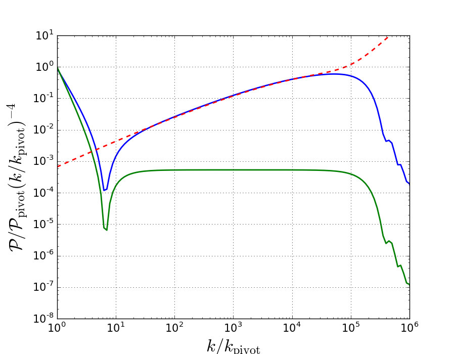
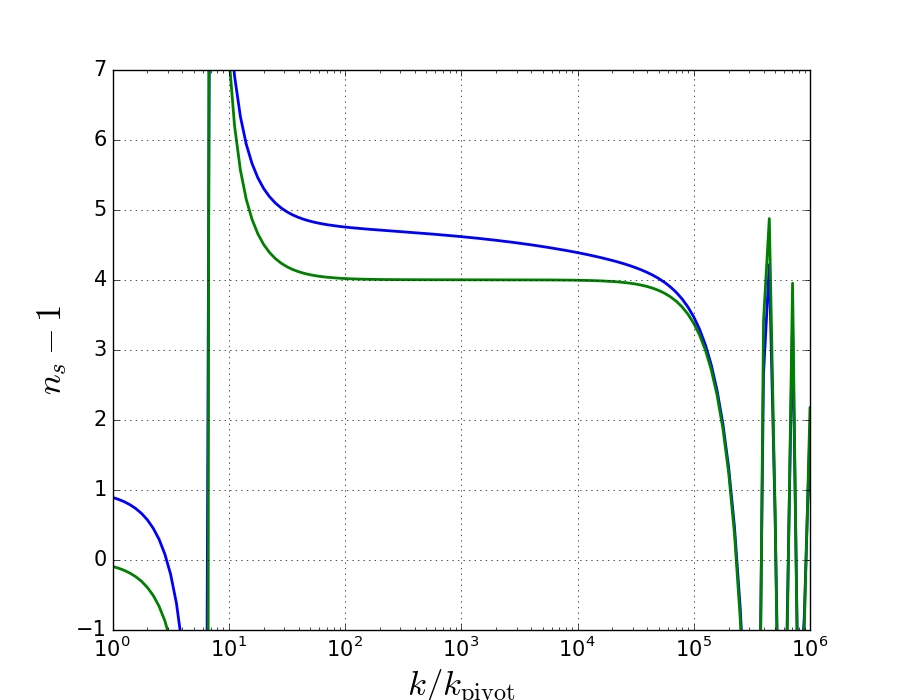
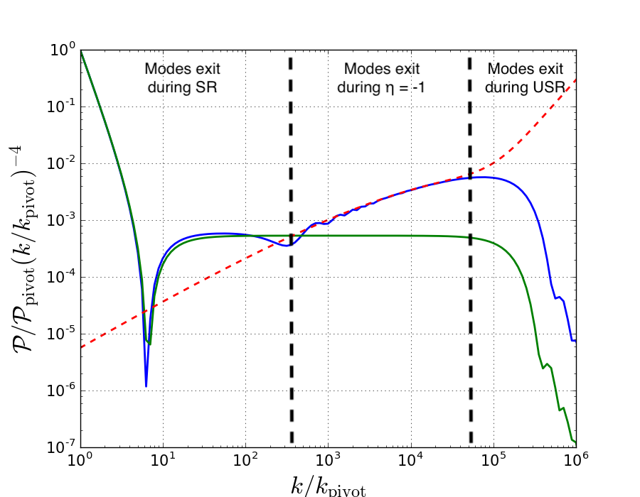
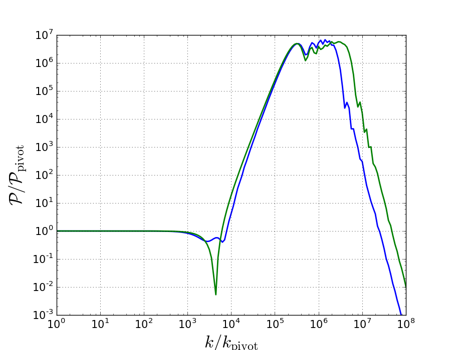
Figure 2: a (top left) compares the power spectra scaled by $k^{4}$ for the transitions $\eta=0\rightarrow\eta=-6$ (green) and $\eta=-1\rightarrow\eta=-6$ (blue), showing the steeper growth possible for the latter case. The duration of the USR stage was chosen to make the dip in the two spectra match. The figure also shows the $k^{5}|(0.1+1.6i)-\log k|^{2}$ scale dependence (red dashed line), which comes from using Eq. (16) to do the matching (see text below Eq. (16)); b (top right) shows the spectral index for these cases; c (bottom left) compares the power spectra scaled by $k^{4}$ for the transitions $\eta=0\rightarrow\eta=-6$ (green) and $\eta=0\rightarrow\eta=-1\rightarrow\eta=-6$ (blue), together with the same approximate scaling as above (red dashed). The dashed lines demarcate the phase in which modes exit for the $\eta=0\rightarrow\eta=-1\rightarrow\eta=-6$ case; d (bottom right) compares the power spectra for the transitions $\eta=0\rightarrow\eta=-6\rightarrow\eta=6$ (green) and $\eta=0\rightarrow\eta=-1\rightarrow\eta=-6\rightarrow\eta=6$ (blue), showing the shorter range of scales exiting the horizon during the USR stage in the latter case.

We can clearly see that the spectral index is larger than $4$ for this new transition and that it matches the approximate $k^{5}(\log k)^{2}$ form predicted above. This demonstrates again the point that the scaling of the steep growth is determined by the $k$ dependence of the sub-leading term in an expansion for modes exiting before the USR stage. We also emphasise that although not of power law form, this behaviour is sustained over a large range of scales (i.e. not a transitory growth caused, for example, by the cancellation of two terms in an asymptotic expansion, as occurs after the dip) just like the $k^{4}$ growth. This is the steepest sustained growth we could find in all cases tested. We have verified that the scale dependence does not change for transitions into stages other than USR (i.e. $\eta=-5$ or $\eta=-4$), as was also the case for the results of Ref. Byrnes et al. (2019), which we again stress is expected since the form of the spectrum is determined by the modes exiting before the transition. Finally we investigated examples with many different $\eta$ values in the pre-transition phase. In all cases the scale dependence of the spectra matches the expectations of the argument of section II.2.

It is well known that for scales that are observed in the Cosmic Microwave Background (CMB) the spectrum must be approximately scale-invariant and hence a stage with $\eta\approx 0$ is always required. To present a more realistic example of a growth steeper than $k^{4}$ therefore, we considered multiple transitions, such as $\eta=0\rightarrow\eta=-1\rightarrow\eta=-6$. In this case one still expects modes which exit the horizon during the $\eta=-1$ phase to have a steeper than $k^{4}$ dependence assuming USR lasts long enough. We tested this scenario by having a $\eta=0\rightarrow\eta=-1$ transition at $\tau_{1,2}=-500$ and a second $\eta=-1\rightarrow\eta=-6$ transition at $\tau_{2,3}=-1$. We show the results in Fig. (2c). For the parameters chosen, the scales exiting the horizon during the $\eta=-1$ stage are all enhanced by the subsequent USR stage giving a $k^{5}(\log k)^{2}$ type scaling, while the final modes that crossed the horizon during the slow-roll stage ($\eta=0$) are also enhanced but give rise to a $k^{4}$ scaling. Here the duration of the USR phase is once again extremely important. The approximate dependence of the scale of the dip, $k_{\text{dip}}$, with the duration of the USR stage remains $k_{\rm dip}\approx\tau_{\text{USR}}^{-3/2}k_{\rm peak}$. This is because the time dependence of the decaying mode during $\eta=-1$ differs only logarithmically when compared with the slow-roll phase, and at a slow-roll to $\eta=-1$ transition the decaying mode in slow-roll is matched to decaying mode of the $\eta=-1$ phase. Assuming USR is long enough for $k_{\rm dip}$ to correspond to scales which crossed the horizon during slow-roll, as in Fig. (2c), the $k^{4}$ dependence is seen for slightly shorter scales, followed by a transition to $k^{5}(\log k)^{2}$ type scaling at $k_{\rm trans}\approx\tau_{1,2}^{-1}$.

IV Decay of the spectrum

A key difference between the slow-roll to USR transition and the case with an intermediate $\eta=-1$ phase, is that the steeper growth that this phase allows means that the USR stage can be shorter for the same overall growth. In Fig. (2d), we illustrate this point with an example where the parameters have been chosen to maximise the range of scales affected by the $k^{5}(\log k)^{2}$ spectrum. In this case, the duration of the USR is now $\approx 1.65$ e-folds compared with $\approx 2.3$ e-folds for the pure slow-roll to USR case (calculated using the full matching).

We now stress a second important consequence of the essential USR stage. During USR, modes still exit the horizon with an approximately scale-invariant spectrum. After the spectrum has reached its maximum, therefore, a non-negligible range of scales must be approximately scale-invariant and the spectrum can only decay for smaller scales than that – i.e. even if the spectrum were to decay arbitrary quickly after the USR stage, there would still be a range of scale-invariant modes after the steep rise. In the case with an $\eta=-1$ stage presented in Fig. (2d), this range of scales can be reduced by a third.

The impossibility of the spectrum decaying immediately after reaching the maximum is expected to have an effect on primordial black hole constraints similar to those derived from the steepest possible growth by Byrnes et al.Byrnes et al. (2019), since narrow gaps in PBH parameter space are more difficult to accommodate. We emphasise that the fact that the $\eta=-1$ phase allows for both a steeper growth and decay alleviates slightly these constraints when compared to the pure $\eta=0$ case. It should be noted, however, that in the presence of a stage of $\eta=-2$ the required duration of the USR stage can be reduced even further while keeping the $k^{4}$ spectral growth. This is because the decaying mode during the $\eta=-2$ stage decays more slowly than in the $\eta>-2$ cases and thus needs less growth during USR to achieve the same amplitude.

V Effect on the spectral index on large scales

A further consequence of the generation of steep growth on short scales is a modification of the spectral index of larger scales – even those larger than $k_{\rm dip}$. Since there exist excellent constraints on the spectral index, $n_{\rm s}-1={\rm d}\log{\cal P}_{\cal R}/{\rm d}\log k$, and the running, $\alpha_{\rm s}={\rm d}n_{\rm s}/{\rm d}\log k$, on CMB scales, one can estimate how far the peak of the spectrum has to be from these scales in order not to significantly effect model constraints.

Considering the slow-roll to USR case we can use Eq. (13) to estimate the contamination in the spectral index due to an USR stage. One finds $\Delta n_{\rm s}\approx-\tau_{USR}^{3}k^{2}/k^{2}_{\rm peak}$. This can be compared to the observational uncertainty in $n_{\rm s}$: $\sigma_{n_{\rm s}}=0.0042$ Akrami et al. (2018). For a USR phase that gives a seven order of magnitude growth in the power spectrum, we find modes satisfying $\log_{10}(k_{\rm peak}/k)\lessapprox 3$ are significantly affected (i.e. $\Delta n_{\rm s}>\sigma_{n_{\rm s}}$). Using the matching of the full unexpanded solution we find the more precise condition $\log_{10}(k_{\rm peak}/k)\lessapprox 3.35$, and repeating the calculation for the running, where $\sigma_{\alpha_{\rm s}}=0.0067$, we find $\log_{10}(k_{\rm peak}/k)\lessapprox 3.40$.

VI Isocurvature modes

In a multi-field scenario, entropy fluctuations may be generated that can then be converted to curvature perturbations either during or at the end of inflation. When this conversion takes place, the spectrum in the isocurvature sector is inherited by the resulting contribution to ${\cal R}$. It is thus conceivable that if isocurvature modes can have a steeper spectrum than $k^{5}(\log k)^{2}$, a steeper spectrum in ${\cal R}$ could ultimately be achieved. We give preliminary consideration to this idea by considering a nearly massless (spectator) isocurvature mode for which the Sasaki-Mukhanov equation takes the form

$$v_{s}^{\prime\prime}+\left(k^{2}-a^{2}H^{2}(2-\epsilon)\right)v_{s}=0\,.$$ (22)

During slow-roll inflation this equation implies that the entropy $S\equiv v_{s}/z$ is conserved on super-horizon scales, with $z$ given by Eq. (2). If there is then a transition to a USR phase or similar, $S$ will grow in a similar way to ${\cal R}$, and one might think that a matching between the two phases would allow the scale-dependence of the sub-leading term in an expansion of $S$ before the transition to be imprinted on the growing mode after the transition. This cannot occur, however, because unlike in the adiabatic case for ${\cal R}$, the boundary conditions for isocurvature modes imply that $v_{s}$ and its first derivative must be continuous, and not the derivative of $S$. Moreover, because $\eta$ does not enter the Sasaki-Mukhanov equation for $v_{s}$, if there is a sharp transition, for example from slow-roll to USR, its solution is practically unchanged. It is therefore not possible for the solution after the transition to capture the scale-dependence of the decaying component of the pre-transition solution, and the USR phase simply enhances the power spectrum with scale-dependence fixed by the leading term before the transition.

One could also relax the assumption that the isocurvature field is a pure spectator and allow a fast transition in its mass, as studied in Ref. Carrilho and Ribeiro (2017). A transition which increases the mass parameter does give rise to a blue spectrum for scales exiting the horizon after the transition, but one limited by $k^{3}$. Moreover, it also induces a decay of its overall amplitude in time, except in the contrived case in which this transition in the mass is simultaneous with a transition from slow-roll to USR.

More complicated multi-field scenarios may generate steeper spectra, but are beyond the scope of this work.

VII Conclusions

We have revisited the question of how steeply the power spectrum from single field inflation can grow with scale. Our first main result was to show that the ultimate scale-dependence of scales which exit the horizon during inflation requires us to consider the leading and sub-leading terms in an asymptotic expansion of modes normalised to the Bunch-Davis vacuum. If there is a transition during inflation to a phase with a growing solution (in time) such as USR, the scale-dependence of the sub-leading (decaying) mode for scales which exited the horizon before the transition is inherited by the growing mode after the transition. If USR lasts sufficiently long for the growing mode to become dominant over a range of scales, these scales exhibit a steeply growing spectrum. This insight allowed us to quickly recover the result that a phase of USR inflation after slow-roll inflation can cause the modes which exit the horizon towards the end of the slow-roll phase to gain a $k^{4}$ dependence, and led us to our second main result. This was to show that $k^{4}$ is not the steepest sustained growth that is possible, and that a phase in which $\eta=-1$ followed by a USR phase leads to a $k^{5}(\log k)^{2}$ type growth, which can in principle be sustained for an arbitrary large range of scales.

We also considered over what range of scales the power spectrum must remain large for after a steep growth and showed this can be reduced in cases with the steeper $k^{5}(\log k)^{2}$ growth. Finally, we considered over what range of scales $n_{\rm s}$ and $\alpha_{\rm s}$ for modes which exit during slow-roll are significantly affected by a subsequent USR phase, and asked whether isocurvature modes could give rise to an even steeper growth than $k^{5}(\log k)^{2}$, which we found was likely not possible. We conclude that $k^{5}(\log k)^{2}$ appears to be the steepest sustained growth of the power spectrum that can be achieved for inflation with canonical scalar fields, and that both this steeper than $k^{4}$ growth, and subsequent swifter decay, could be helpful in avoiding constraints on the formation of PBHs.

Appendix A Intermediate cases

In this appendix, we explore transitions including alternative pre-USR stages not shown in the main text, including scenarios with non-integer values of $\eta$. Our aim is to clearly demonstrate that the spectral index of the decaying term, as shown in Eq. (15), is always imprinted on the growing mode that generates the steepest part of the spectrum, giving a spectral index of $2\alpha+3=5-|\eta+1|$. We plot our results in Fig. (3), in which we can see that the expectations from Eq. (15), hold for almost all cases, including the prediction that the spectral index is the same for situations in which $|\eta+1|$ is the same. For $\eta$ approaching $-1$, the results deviate from a constant spectral index, since higher order terms in a power-series expansion become important. However, the sub-leading term is still a good approximation for scales sufficiently distant from the peak, as can be seen for the cases with $\eta=-1/2$ and $\eta=-3/2$ (superimposed on the right-hand plot). In the $\eta=-1$ limit the power-series expansion breaks down, and many higher order terms effectively contribute and sum to give the logarithmic dependence described in the main text.

 

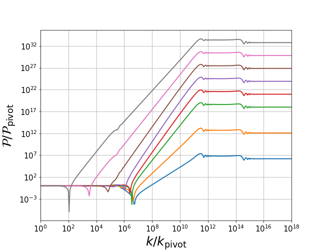
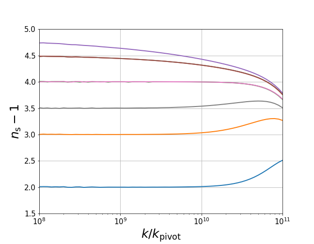
Figure 3: Plots of the power spectra (left) and spectral indices (right) for the transitions $\eta=0\rightarrow\eta=\eta_{t}\rightarrow\eta=-6\rightarrow\eta=0$, with $\eta_{t}=2,1,0,-1/2,-1,-3/2,-2,-5/2$ (from bottom to top on the left plot). Situations with the same spectral index appear superimposed on the plot on the right, so the lines shown correspond to $\eta_{t}=2,1,-5/2,-2,-3/2,-1$ (from bottom to top), but include as well $\eta_{t}=0$ and $\eta_{t}=-1/2$ in the same positions as $\eta_{t}=-2$ and $\eta_{t}=-3/2$, respectively.

References

- Byrnes et al. (2019) C. T. Byrnes, P. S. Cole, and S. P. Patil, JCAP 1906, 028 (2019), eprint 1811.11158.
- Abbott et al. (2016) B. P. Abbott et al. (LIGO Scientific, Virgo), Phys. Rev. Lett. 116, 061102 (2016), eprint 1602.03837.
- Abbott et al. (2018a) B. P. Abbott et al. (LIGO Scientific, Virgo) (2018a), eprint 1811.12940.
- Abbott et al. (2018b) B. P. Abbott et al. (LIGO Scientific, Virgo) (2018b), eprint 1811.12907.
- Carr and Hawking (1974) B. J. Carr and S. W. Hawking, Mon. Not. Roy. Astron. Soc. 168, 399 (1974).
- Bird et al. (2016) S. Bird, I. Cholis, J. B. Muñoz, Y. Ali-Haïmoud, M. Kamionkowski, E. D. Kovetz, A. Raccanelli, and A. G. Riess, Phys. Rev. Lett. 116, 201301 (2016), eprint 1603.00464.
- Sasaki et al. (2016) M. Sasaki, T. Suyama, T. Tanaka, and S. Yokoyama, Phys. Rev. Lett. 117, 061101 (2016), [erratum: Phys. Rev. Lett.121,no.5,059901(2018)], eprint 1603.08338.
- Carr et al. (2016) B. Carr, F. Kuhnel, and M. Sandstad, Phys. Rev. D94, 083504 (2016), eprint 1607.06077.
- Carr et al. (2017) B. Carr, M. Raidal, T. Tenkanen, V. Vaskonen, and H. Veermäe, Phys. Rev. D96, 023514 (2017), eprint 1705.05567.
- Zaballa et al. (2007) I. Zaballa, A. M. Green, K. A. Malik, and M. Sasaki, JCAP 0703, 010 (2007), eprint astro-ph/0612379.
- Josan et al. (2009) A. S. Josan, A. M. Green, and K. A. Malik, Phys. Rev. D79, 103520 (2009), eprint 0903.3184.
- Cole and Byrnes (2018) P. S. Cole and C. T. Byrnes, JCAP 1802, 019 (2018), eprint 1706.10288.
- Germani and Prokopec (2017) C. Germani and T. Prokopec, Phys. Dark Univ. 18, 6 (2017), eprint 1706.04226.
- Germani and Musco (2019) C. Germani and I. Musco, Phys. Rev. Lett. 122, 141302 (2019), eprint 1805.04087.
- Carr et al. (2010) B. J. Carr, K. Kohri, Y. Sendouda, and J. Yokoyama, Phys. Rev. D81, 104019 (2010), eprint 0912.5297.
- Ananda et al. (2007) K. N. Ananda, C. Clarkson, and D. Wands, Phys. Rev. D75, 123518 (2007), eprint gr-qc/0612013.
- Baumann et al. (2007) D. Baumann, P. J. Steinhardt, K. Takahashi, and K. Ichiki, Phys. Rev. D76, 084019 (2007), eprint hep-th/0703290.
- Alabidi et al. (2012) L. Alabidi, K. Kohri, M. Sasaki, and Y. Sendouda, JCAP 1209, 017 (2012), eprint 1203.4663.
- Di and Gong (2018) H. Di and Y. Gong, JCAP 1807, 007 (2018), eprint 1707.09578.
- Kohri and Terada (2018) K. Kohri and T. Terada, Phys. Rev. D97, 123532 (2018), eprint 1804.08577.
- Clesse et al. (2018) S. Clesse, J. García-Bellido, and S. Orani (2018), eprint 1812.11011.
- Ballesteros and Taoso (2018) G. Ballesteros and M. Taoso, Phys. Rev. D97, 023501 (2018), eprint 1709.05565.
- Cheng et al. (2019) S.-L. Cheng, W. Lee, and K.-W. Ng, Phys. Rev. D99, 063524 (2019), eprint 1811.10108.
- Bhaumik and Jain (2019) N. Bhaumik and R. K. Jain (2019), eprint 1907.04125.
- Malik and Wands (2009) K. A. Malik and D. Wands, Phys. Rept. 475, 1 (2009), eprint 0809.4944.
- Dias et al. (2016) M. Dias, J. Frazer, D. J. Mulryne, and D. Seery, JCAP 1612, 033 (2016), eprint 1609.00379.
- Mulryne and Ronayne (2016) D. J. Mulryne and J. W. Ronayne (2016), eprint 1609.00381.
- Ronayne and Mulryne (2018) J. W. Ronayne and D. J. Mulryne, JCAP 1801, 023 (2018), eprint 1708.07130.
- Seery (2016) D. Seery (2016), eprint 1609.00380.
- Butchers and Seery (2018) S. Butchers and D. Seery, JCAP 1807, 031 (2018), eprint 1803.10563.
- Israel (1966) W. Israel, Nuovo Cim. B44S10, 1 (1966), [Nuovo Cim.B44,1(1966)].
- Deruelle and Mukhanov (1995) N. Deruelle and V. F. Mukhanov, Phys. Rev. D 52, 5549 (1995).
- Passaglia et al. (2019) S. Passaglia, W. Hu, and H. Motohashi, Phys. Rev. D99, 043536 (2019), eprint 1812.08243.
- Akrami et al. (2018) Y. Akrami et al. (Planck) (2018), eprint 1807.06211.
- Carrilho and Ribeiro (2017) P. Carrilho and R. H. Ribeiro, Phys. Rev. D95, 043516 (2017), eprint 1612.00035.