Gain with no Pain: Efficient Kernel-PCA by Nyström Sampling

Abstract

In this paper, we propose and study a Nyström based approach to efficient large scale kernel principal component analysis (PCA). The latter is a natural nonlinear extension of classical PCA based on considering a nonlinear feature map or the corresponding kernel. Like other kernel approaches, kernel PCA enjoys good mathematical and statistical properties but, numerically, it scales poorly with the sample size. Our analysis shows that Nyström sampling greatly improves computational efficiency without incurring any loss of statistical accuracy. While similar effects have been observed in supervised learning, this is the first such result for PCA. Our theoretical findings, which are also illustrated by numerical results, are based on a combination of analytic and concentration of measure techniques. Our study is more broadly motivated by the question of understanding the interplay between statistical and computational requirements for learning.

1 Introduction

Achieving good statistical accuracy under budgeted computational resources is a central theme in modern machine learning (Bottou and Bousquet,, 2008). Indeed, the problem of understanding the interplay and trade-offs between statistical and computational requirements has recently received much attention. Nonparametric learning, and in particular kernel methods, have provided a natural framework to pursue these questions, see e.g.(Musco and Musco,, 2017; Rudi et al.,, 2015; Alaoui and Mahoney,, 2014; Bach,, 2013; Calandriello et al.,, 2018; Orabona et al.,, 2008). On the one hand, these methods are developed in a sound mathematical setting and their statistical properties are well studied. On the other hand, from a numerical point of view, they scale poorly to large scale problems, and hence improved computational efficiency is of particular interest.

While initial studies have mostly focused on approximating kernel matrices (Drineas and Mahoney,, 2005; Gittens and Mahoney,, 2013; Jin et al.,, 2013), recent results have highlighted the importance of considering downstream learning tasks, if the interplay between statistics and computation is of interest. In particular, results in supervised learning have shown there are regimes where computational gains can be achieved with no loss of statistical accuracy (Rudi et al.,, 2015; Rudi and Rosasco,, 2017). A basic intuition is that approximate computations provide a form of implicit regularization, hence memory and time requirements can be tailored to statistical accuracy allowed by the data (Rudi et al.,, 2015). To which extent similar effects occur beyond supervised learning is unclear. Indeed, the only result in this direction was recently shown for kernel k-means in (Calandriello et al.,, 2018).

In this paper, we consider one of the most basic unsupervised approaches, namely PCA, or rather its nonlinear version, that is kernel PCA (Schölkopf et al.,, 1998). We develop a computationally efficient approximate kernel PCA algorithm using the Nyström method (Williams and Seeger,, 2001) with $m$ sub-samples (NY-KPCA) and show its time complexity to be $O(nm^{2}+m^{3})$ with a space complexity of $O(m^{2})$, in contrast to $O(n^{3})$ and $O(n^{2})$ time and space complexities of KPCA, where $n$ is the sample size. Our main contribution is the analysis of NY-KPCA in terms of finite sample bounds on the reconstruction error of the corresponding $\ell$-dimensional eigenspace (see Theorem 4.1 and related Corollaries 4.2 and 4.3). In particular, we show that NY-KPCA can achieve the same error of KPCA with $m<n$, thereby demonstrating computational gains can occur at no statistical loss. Moreover, we show that adaptive sampling using leverage scores (Alaoui and Mahoney,, 2014) can lead to further gains. More precisely, we show that the requirement on $m$ varies between $(\log n)^{2}$ and $n^{\theta}\log n$ ($\theta<1$) depending on the size of $\ell$, the rate of decay of eigenvalues of the covariance operator and the type of subsampling. Finally, we also present some simple numerical results to corroborate our theoretical results.

We note that some recent papers, see (Sriperumbudur and Sterge,, 2018; Ullah et al.,, 2018), have considered the problem of deriving efficient kernel PCA approximations using random features (Rahimi and Recht,, 2008). However, the notion of reconstruction error considered in these works is different from that of KPCA (Shawe-Taylor et al.,, 2005; Blanchard et al.,, 2007). The reason for a different notion of reconstruction error is to handle certain technicalities that arise in random feature approximation. As a consequence, these results are not directly comparable to our current work and KPCA. In contrast, our results based on Nyström approximation are directly comparable to that of KPCA, wherein we show that the proposed NY-KPCA has similar statistical behavior but better computational complexity than KPCA.

The paper is organized as follows. Relevant notations and definitions are collected in Section 2. Section 3 provides preliminaries on KPCA along with the list of assumptions that will be used throughout the paper. Approximate KPCA using Nyström method is presented in Section 3.2 and the main results of computational vs. statistical tradeoff for NY-KPCA are presented in Section 4. Missing proofs of the results are provided in the appendix.

2 Definitions and Notation

For $\bm{a}:=(a_{1},\ldots,a_{d})\in\mathbb{R}^{d}$ and $\bm{b}:=(b_{1},\ldots,b_{d})\in\mathbb{R}^{d}$ define $\|\bm{a}\|_{2}:=\sqrt{\sum^{d}_{i=1}a^{2}_{i}}$ and $\langle\bm{a},\bm{b}\rangle_{2}:=\sum^{d}_{i=1}a_{i}b_{i}$. $\bm{a}\otimes_{2}\bm{b}:=\bm{a}\bm{b}^{\top}$ denotes the tensor product of $\bm{a}$ and $\bm{b}$. $\mathbf{I}_{n}$ denotes an $n\times n$ identity matrix. $a\wedge b:=\min(a,b)$ and $a\vee b:=\max(a,b)$. $[n]:=\{1,\ldots,n\}$ for $n\in\mathbb{N}$. For constants $a$ and $b$, $a\lesssim b$ (resp. $a\gtrsim b$) denotes that there exists a positive constant $c$ (resp. $c^{\prime}$) such that $a\leq cb$ (resp. $a\geq c^{\prime}b$). For a random variable $A$ with law $P$ and a constant $b$, $A\lesssim_{p}b$ denotes that for any $\delta>0$, there exists a positive constant $c_{\delta}<\infty$ such that $P(A\leq c_{\delta}b)\geq\delta$.

For $x,y\in H$, a Hilbert space, $x\otimes_{H}y$ is an element of the tensor product space $H\otimes H$ which can also be seen as an operator from $H$ to $H$ as $(x\otimes_{H}y)z=x\langle y,z\rangle_{H}$ for any $z\in H$. $\alpha\in\mathbb{R}$ is called an eigenvalue of a bounded self-adjoint operator $S$ if there exists an $x\neq 0$ such that $Sx=\alpha x$ and such an $x$ is called the eigenvector/eigenfunction of $S$ and $\alpha$. An eigenvalue is said to be simple if it has multiplicity one. For an operator $S:H\rightarrow H$, $\|S\|_{\mathcal{L}^{1}(H)}$, $\|S\|_{\mathcal{L}^{2}(H)}$ and $\|S\|_{\mathcal{L}^{\infty}(H)}$ denote the trace, Hilbert-Schmidt and operator norms of $S$, respectively.

3 Kernel PCA by Nyström Sampling

In this section, we review kernel principal component analysis (KPCA) (Schölkopf et al.,, 1998) in population and empirical settings and introduce approximate kernel PCA using Nyström approximation. We assume the following for the rest of the paper:

Assumption 3.1.

$\mathcal{X}$ is a separable topological space and $(\mathcal{H},k)$ is a separable RKHS of real-valued functions $\mathcal{X}$ with a bounded, continuous, strictly positive definite kernel $k$ satisfying $\sup_{x\in\mathcal{X}}\,k(x,x)=:\kappa<\infty$.

3.1 KPCA and Empirical KPCA

Let $X$ be a zero-mean random variable with law $\mathbb{P}$ defined on $\mathcal{X}$. When $\mathcal{X}=\mathbb{R}^{d}$, classical PCA (Jolliffe,, 1986) finds $\mathbf{a}\in\mathbb{R}^{d}$ such that $\text{Var}\left[\left\langle\mathbf{a},X\right\rangle_{2}\right]$ is maximized, with the constraint $\left\lVert\mathbf{a}\right\rVert_{2}=1$. Defining $C:=\mathbb{E}_{X\sim\mathbb{P}}[XX^{\top}]$, the solution is simply the unit eigenvector of $C$ corresponding to its largest eigenvalue. In practice, PCA is computed by replacing $C$ with an empirical approximation $C_{n}=\frac{1}{n}\sum_{i=1}^{n}X_{i}X_{i}^{\top}$ based on a sample $X_{1},\dots,X_{n}$. Kernel PCA extends this idea to an RKHS, $\mathcal{H}$ defined on $\mathcal{X}$, by finding $f\in\mathcal{H}$ with unit norm such that $\text{Var}[f(X)]$ is maximized. Since $\text{Var}[f(X)]=\langle f,Cf\rangle_{\mathcal{H}}$ assuming $\mathbb{E}[f(X)]=0$ for all $f\in\mathcal{H}$, we have $f^{*}=\arg\sup\{\langle f,Cf\rangle_{\mathcal{H}}:\left\lVert f\right\rVert_{\mathcal{H}}=1\}$ where $C$ is the (uncentered) covariance operator on $\mathcal{H}$ defined as

$$C:=\int_{\mathcal{X}}k(\cdot,x)\otimes_{\mathcal{H}}k(\cdot,x)\,d\mathbb{P}(x).$$ (1)

The boundedness of $k$ in Assumption 3.1 ensures that $C$ is trace class and thus compact. Since $C$ is positive and self-adjoint, the spectral theorem (Reed and Simon,, 1980) gives

$$C=\sum_{i\in I}\lambda_{i}\phi_{i}\otimes_{\mathcal{H}}\phi_{i},$$ (2)

where $(\lambda_{i})_{i\in I}\subset\mathbb{R}^{+}$ are the eigenvalues and $(\phi_{i})_{i\in I}$ are the orthonormal system of eigenfunctions that span $\overline{\mathcal{R}(C)}$ with index set $I$ either being finite or countable, in which case $\lambda_{i}\rightarrow 0$ as $i\rightarrow\infty$. The solution to the KPCA problem is thus the eigenfunction of $C$ corresponding to its largest eigenvalue. We make the following simplifying assumption for ease of presentation.

Assumption 3.2.

The eigenvalues $(\lambda_{i})_{i\in I}$ of $C$ are simple, positive, and w.l.o.g. they satisfy a decreasing rearrangement, i.e., $\lambda_{1}>\lambda_{2},\ldots$

Assumption 3.2 ensures that $(\phi_{i})_{i\in I}$ form an orthonormal basis and the eigenspace corresponding to each $\lambda_{i}$ is one-dimensional. This means the orthogonal projection operator onto the $\ell$-eigenspace of $C$, i.e. span$\{(\phi_{i})_{i=1}^{\ell}\}$, is given by

$$P^{\ell}(C)=\sum_{i=1}^{\ell}\phi_{i}\otimes_{\mathcal{H}}\phi_{i}.$$ (3)

The above construction corresponds to population version of KPCA when the data distribution $\mathbb{P}$ is known. If $\mathbb{P}$ is unknown and the knowledge of $\mathbb{P}$ is available only through the training set $\left(X_{i}\right)_{i=1}^{n}\stackrel{{\scriptstyle i.i.d.}}{{\sim}}\mathbb{P}$, then KPCA cannot be carried out as $C$ depends on $\mathbb{P}$. Therefore, an approximation to $C$ is used to perform KPCA. Most commonly, this approximation is chosen to be the empirical estimator of $C$ defined as

$$C_{n}=\frac{1}{n}\sum_{i=1}^{n}k(\cdot,X_{i})\otimes_{\mathcal{H}}k(\cdot,X_{i})$$ (4)

resulting in empirical kernel PCA (EKPCA). Note that $C_{n}$ is a finite rank, positive, and self-adjoint operator. Thus the spectral theorem (Reed and Simon,, 1980) yields

$$C_{n}=\sum_{i=1}^{n}\hat{\lambda}_{i}\hat{\phi}_{i}\otimes_{\mathcal{H}}\hat{\phi}_{i},$$ (5)

where $(\hat{\lambda}_{i})_{i=1}^{n}\subset\mathbb{R}^{+}$ and $(\hat{\phi}_{i})_{i=1}^{n}\subset\mathcal{H}$ are the eigenvalues and eigenfunctions of $C_{n}$. Similar to Assumption 3.2, we assume the following:

Assumption 3.3.

$\emph{rank}(C_{n})=n$, the eigenvalues $(\hat{\lambda}_{i})_{i=1}^{n}$ of $C_{n}$ are simple and w.l.o.g. they satisfy a decreasing rearrangement, i.e., $\hat{\lambda}_{1}\geq\hat{\lambda}_{2}\geq\ldots$.

The eigensystem $(\hat{\lambda}_{i},\hat{\phi}_{i})_{i=1}^{n}$ of $C_{n}$ can be obtained by solving an $n$-dimensional system involving the eigendecomposition of the Gram matrix $\mathbf{K}=[k(X_{i},X_{j})]_{i,j\in[n]},$ which scales as $O(n^{3})$ (Schölkopf et al.,, 1998). In particular, the eigenvalues of $\mathbf{K}$ are related to those of $C_{n}$ as $\lambda_{i}(\mathbf{K})=n\hat{\lambda}_{i}$. Moreover, if $\mathbf{u}_{i}$ is an orthonormal eigenvector of $\mathbf{K}$ corresponding to the eigenvalue $\lambda_{i}(\mathbf{K})$, then it holds for all $x\in{\mathcal{X}}$,

$$\phi_{i}(x)=\frac{1}{\sqrt{n\hat{\lambda}_{i}}}\sum_{j=1}^{n}k(x,x_{j})u_{i,j}.$$ (6)

The above result proven in (Schölkopf et al.,, 2001) can be seen as a representer theorem (Kimeldorf and Wahba,, 1971) for KPCA. Finally, note that, for some $\ell\leq n$, the orthogonal projection operator onto $\text{span}\{(\hat{\phi}_{i})_{i=1}^{\ell}\}$ is given by

$$P^{\ell}(C_{n})=\sum_{i=1}^{\ell}\hat{\phi}_{i}\otimes_{\mathcal{H}}\hat{\phi}_{i}.$$ (7)

3.2 Approximate Kernel PCA using Nyström Method

For large sample sizes, since performing KPCA is computationally intensive, various approximation schemes that has been explored in the kernel machine literature can be deployed to speed up EKPCA. Recently, one such approximation involving random Fourier features has been studied by Sriperumbudur and Sterge, (2018) and Ullah et al., (2018) to speed EKPCA while maintaining its statistical performance. In this paper, we explore the popular Nyström approximation (Williams and Seeger,, 2001; Drineas and Mahoney,, 2005) to speed up EKPCA and study the trade-offs between computational gains and statistical accuracy. The general idea in Nyström method is to obtain a low-rank approximation to the Gram matrix $\mathbf{K}$, and replace $\mathbf{K}$ by this approximation in kernel algorithms, resulting in computational speedup. Since $\mathbf{K}$ is related to $C_{n}$ (as discussed in Section 3.1), Nyström method can also be seen as obtaining a low rank approximation to $C_{n}$, which is what we exploit in obtaining a Nyström approximate KPCA. It follows from (6) that the eigenfunctions of $C_{n}$ lie in the space

$$\mathcal{H}_{n}=\left\{f\in\mathcal{H}\,\Big{|}\,f=\sum_{i=1}^{n}\alpha_{i}k(\cdot,X_{i}),\alpha_{1},...,\alpha_{n}\in\mathbb{R}\right\}.$$

Therefore, it can be seen that EKPCA is a solution to the following problem

$$\arg\sup\left\{\left\langle f,C_{n}f\right\rangle_{\mathcal{H}}:f\in\mathcal{H}_{n},\,\left\lVert f\right\rVert_{\mathcal{H}}=1\right\},$$

assuming $\mathbf{K}$ is invertible. Extending this representation, we propose Nyström KPCA (NY-KPCA) as a solution to the following problem:

$$\arg\sup\left\{\left\langle f,C_{n}f\right\rangle_{\mathcal{H}}:f\in\mathcal{H}_{m},\,\left\lVert f\right\rVert_{\mathcal{H}}=1\right\},$$ (8)

where

$$\mathcal{H}_{m}=\left\{f\in\mathcal{H}\,\Big{|}\,f=\sum_{i=1}^{m}\alpha_{i}k(\cdot,\tilde{X}_{i}),\alpha_{1},...,\alpha_{m}\in\mathbb{R}\right\}$$

is a low-dimensional subspace of $\mathcal{H}_{n}$ and $\{\tilde{X}_{1},...,\tilde{X}_{m}\}$ is a subset of the training set with $\tilde{X}_{i}$’s being distinct. Basically, we are considering a plain Nyström approximation where the points $\{\tilde{X}_{1},\ldots,\tilde{X}_{m}\}$ are sampled uniformly without replacement from $\{X_{1},\ldots,X_{n}\}$, however, other subsampling methods are possible, see Section 3.2.1. The following result, which is proved in the supplement (see Section 6.1), shows that the solution to (8) is obtained by solving a finite dimensional linear system, which has better computational complexity than that of EKPCA. To this end, we first introduce some notation, $\mathbf{K}_{mm}=[k(\tilde{X_{i}},\tilde{X_{j}})]_{i,j\in[m]}\text{, }\mathbf{K}_{nm}=[k(X_{i},\tilde{X_{j}})]_{i\in[n],j\in[m]}\in\mathbb{R}^{n\times m},\mathbf{K}_{mn}=\mathbf{K}_{nm}^{\top}.$

Proposition 3.4.

Define the $m\times m$ matrix $\mathbf{M}=\mathbf{K}_{mm}^{-1/2}\mathbf{K}_{mn}\mathbf{K}_{nm}\mathbf{K}_{mm}^{-1/2}$. The solution to (8) is given by

$$\hat{\phi}_{1,m}=\tilde{Z}_{m}^{*}\mathbf{K}_{mm}^{-1/2}\mathbf{u}_{1,m},$$

where $\mathbf{u}_{1,m}$ is the eigenvector of $\frac{1}{n}\mathbf{M}$ corresponding to its largest eigenvalue and $\tilde{Z}_{m}^{*}:\mathbb{R}^{m}\rightarrow\mathcal{H},\,\bm{\alpha}\mapsto\sum_{i=1}^{m}\alpha_{i}k(\cdot,\tilde{X}_{i}).$

The cost of computing $\mathbf{M}$ is $O(nm^{2}+m^{3})$ and the cost of computing its eigendecomposition is $O(m^{3})$. Thus, for $m<n$, the cost of NY-KPCA scales as $O(nm^{2})$, faster than the $O(n^{3})$ cost of EKPCA. Define

$$\tilde{\mathbf{K}}:=\mathbf{K}_{nm}\mathbf{K}_{mm}^{-1}\mathbf{K}_{mn},$$ (9)

which is called the Nyström approximation (Williams and Seeger,, 2001; Drineas and Mahoney,, 2005) to the Gram matrix $\mathbf{K}$. It is easy to verify that $\mathbf{M}$ and $\tilde{\mathbf{K}}$ have same eigenvalues since $\mathbf{M}=\mathbf{K}_{mm}^{-1/2}\mathbf{K}_{mn}\left(\mathbf{K}_{mm}^{-1/2}\mathbf{K}_{mn}\right)^{\top}$ and $\tilde{\mathbf{K}}=\left(\mathbf{K}_{mm}^{-1/2}\mathbf{K}_{mn}\right)^{\top}\mathbf{K}_{mm}^{-1/2}\mathbf{K}_{mn}$, and rank$(\mathbf{M})=\text{rank}(\tilde{\mathbf{K}})$. Therefore we work with $\tilde{\mathbf{K}}$ and make the following assumption on its eigenvalues.

Assumption 3.5.

$\emph{rank}(\tilde{\mathbf{K}})=m$. The eigenvalues $(\hat{\lambda}_{i,m})_{i=1}^{m}$ of $\frac{1}{n}\tilde{\mathbf{K}}$ are simple and w.l.o.g. they satisfy a decreasing rearrangement, i.e., $\hat{\lambda}_{1,m}>\hat{\lambda}_{2,m}\ldots>\hat{\lambda}_{m,m}$.

The symmetry of $\mathbf{M}$ guarantees orthonormality of $(\mathbf{u}_{i,m})_{i}$, and the orthonormality of $(\hat{\phi}_{i,m})_{i}$ follows. For some $\ell\leq m$, the orthogonal projector onto span$\{\hat{\phi}_{i,m}\}_{i=1}^{\ell}$ is given by

$$P^{\ell}_{m}(C_{n})=\sum_{i=1}^{\ell}\hat{\phi}_{i,m}\otimes_{\mathcal{H}}\hat{\phi}_{i,m}.$$ (10)

One may ask if $\hat{\phi}_{i,m}$ are eigenfunctions of some operator on $\mathcal{H}$. Denote $P_{m}$ as the orthogonal projector onto $\mathcal{H}_{m}$. It is simple to verify (Rudi et al.,, 2015, Theorem 2) that $P_{m}=\tilde{Z}_{m}^{*}\mathbf{K}_{mm}^{-1}\tilde{Z}_{m}$ and that $\left(\hat{\lambda}_{i,m},\hat{\phi}_{i,m}\right)$ are the orthonormal eigenfunctions of $P_{m}C_{n}P_{m}$, i.e.,

$$P_{m}C_{n}P_{m}\hat{\phi}_{i,m}=\hat{\lambda}_{i,m}\hat{\phi}_{i,m}\text{ for all }i\in[m].$$ (11)

Therefore, we may think of $P_{m}C_{n}P_{m}$ as a low-rank approximation to $C_{n}$.

3.2.1 Approximate Leverage Scores

In the above discussion on Nyström KPCA, $\tilde{\mathbf{X}}:=\{\tilde{X}_{1},\ldots,\tilde{X}_{m}\}$ is a subset of the training set $\mathbf{X}:=\{X_{1},\ldots,X_{n}\}$ with the entries of $\tilde{\mathbf{X}}$ being sampled uniformly without repetition from $\mathbf{X}$. As an alternative to uniform sampling, $\tilde{\mathbf{X}}$ can be sampled according to the leverage score distribution (Alaoui and Mahoney,, 2015; Drineas et al.,, 2012; Cohen et al.,, 2015). For any $s>0$, the leverage scores associated with the training data $\mathbf{X}$ are defined as

$$(l_{i}(s))_{i=1}^{n}\,,\quad l_{i}(s)=[\mathbf{K}(\mathbf{K}+ns\mathbf{I}_{n})^{-1}]_{ii}\,,i\in[n]$$

with the leverage score distribution being $p_{i}(s)=\frac{l_{i}(s)}{\sum^{n}_{i=1}l_{i}(s)}$ according to which $\mathbf{X}$ can be sampled independently with replacement to achieve $\tilde{\mathbf{X}}$. Since the leverage scores are computationally intensive to compute, usually, they are approximated and one such approximation is $T$-approximate leverage scores.

Definition 3.6.

($T$-approximate leverage scores) For a given $s>0$, let $(l_{i}(s))_{i=1}^{n}$ be the leverage scores associated with the training data $\{X_{1},...,X_{n}\}$. Let $\delta>0$, $s_{0}>0$, and $T\geq 1$. $(\hat{l}_{i}(s))_{i=1}^{n}$ are $T$-approximate leverage scores, with confidence $\delta$, if the following holds with probability at least $1-\delta$:

$$\frac{1}{T}l_{i}(s)\leq\hat{l}_{i}(s)\leq\,Tl_{i}(s),\quad\forall i\in[n],\quad s>s_{0}.$$

Given $T$-approximate leverage scores for $s>s_{0}$, $\tilde{\mathbf{X}}$ can be obtained by sampling $\mathbf{X}$ with replacement according to the sampling distribution $\hat{p}_{i}(s)=\hat{l}_{i}(s)/\sum_{i=1}^{n}\hat{l}_{i}(s)$. Having obtained $\tilde{\mathbf{X}}$, (8) can be solved exactly as in Proposition 3.4. We refer to this method as approximate leverage score (ALS) Nyström subsampling.

4 Computational vs. Statistical Trade-Off: Main Results

As shown in the earlier section, Nyström kernel PCA approximates the solution to empirical kernel PCA with less computational expense. In this section, we explore whether this computational saving is obtained at the expense of statistical performance. As in Sriperumbudur and Sterge, (2018), we measure the statistical performance of KPCA, EKPCA, and NY-KPCA in terms of reconstruction error. In linear PCA, the reconstruction error, given by

$$\mathbb{E}_{X\sim\mathbb{P}}\left\lVert\left(I-P^{\ell}(C)\right)X\right\rVert_{2}^{2},$$ (12)

is the error involved in reconstructing a random variable $X$ by projecting it onto the $\ell$-eigenspace (i.e., span of the top-$\ell$ eigenvectors) associated with its covariance matrix, $C=\mathbb{E}[XX^{\top}]$ through the orthogonal projection operator $P^{\ell}(C)$. Clearly, the error is zero when $\ell=d$. The analog of the reconstruction error in KPCA, as well as EKPCA and NY-KPCA, can be similarly stated in terms of their projection operators, (3), (7), and (10) as follows. For any orthogonal projection operator $P:{\mathcal{H}}\to{\mathcal{H}}$, define the reconstruction error as

$$R(P):=\mathbb{E}_{X\sim\mathbb{P}}\left\lVert\left(I-P\right)k(\cdot,X)\right\rVert_{\mathcal{H}}^{2}.$$

For the linear kernel this exactly the reconstruction error of PCA. In the following, we often make use of the following identity

$$R(P)=\|(I-P)C^{1/2}\|^{2}_{{\mathcal{L}^{2}(\mathcal{H})}},$$ (13)

for which we report a proof in the supplement (see Section 6.2). Based on this definition, the reconstruction error in KPCA, EKPCA and NY-KPCA are given by

$$R_{C,\ell}:=R(P^{\ell}(C)),\,\,R_{C_{n},\ell}:=R(P^{\ell}(C_{n})),\,\,\text{and}\,\,R^{nys}_{C_{n},\ell}:=R(P^{\ell}_{m}(C_{n}))$$ (14)

respectively. The following theorem, proved in the supplement (see Section 6.3), provides finite-sample bounds on the reconstruction error associated with NY-KPCA, under both uniform and approximate leverage score subsampling, from which convergence rates may be obtained.

Theorem 4.1.

Suppose Assumptions 3.1-3.5 hold. For any $t>0$, define $\mathcal{N}_{C}(t)=\emph{tr}((C+tI)^{-1}C)$ and $\mathcal{N}_{C,\infty}(t)=\sup_{x\in\mathcal{X}}\langle k(\cdot,x),(C+tI)^{-1}k(\cdot,x)\rangle_{\mathcal{H}}$. Then the following hold:
(i) Suppose $n>3$, $0<\delta<1$, $\frac{9\kappa}{n}\log\frac{n}{\delta}\leq t\leq\lambda_{1}$, and $m\geq\left(67\vee 5\mathcal{N}_{C,\infty}(t)\right)\log\frac{4\kappa}{t\delta}$. Then, for plain Nyström subsampling:

$$\mathbb{P}^{n}\left\{(X_{i})^{n}_{i=1}:R_{C_{n},\ell}^{nys}\leq\mathcal{N}_{C}(t)\left(6\lambda_{\ell}+42t\right)\right\}\geq 1-2\delta.$$ (15)

(ii) For $0<\delta<1$, suppose there exists $T\geq 1$ such that $(\hat{l}_{i}(s))_{i=1}^{n}$ are $T-$approximate leverage scores with confidence $\delta$ for any $t\geq\frac{19\kappa}{n}\log\frac{2n}{\delta}$. Assume approximate leverage score Nyström subsampling is used with

$$t=\min\left\{\frac{19\kappa}{n}\log\frac{2n}{\delta}\leq t\leq\lambda_{1}\,\Big{|}\,78T^{2}\mathcal{N}_{C}(t)\log\frac{8n}{\delta}\leq m\right\}.$$

If $n\geq 1655\kappa+223\kappa\log\frac{2\kappa}{\delta}$ and $m\geq 334\log\frac{8n}{\delta}$, then

$$\mathbb{P}^{n}\left\{(X_{i})^{n}_{i=1}:R_{C_{n},\ell}^{nys}\leq\mathcal{N}_{C}(t)\left(6\lambda_{\ell}+42t\right)\right\}\geq 1-3\delta.$$ (16)

To understand the significance of Theorem 4.1, we have to compare it to the behavior of the reconstruction error associated with EKPCA, i.e., $R_{C_{n},\ell}$. (Rudi et al.,, 2015, Theorem 3.1) showed that for $n>3$, $0<\delta<1$ and $\frac{9\kappa}{n}\log\frac{n}{\delta}\leq t\leq\lambda_{1}$,

$$\mathbb{P}^{n}\left\{(X_{i})^{n}_{i=1}:R_{C_{n},\ell}\leq 9\mathcal{N}_{C}(t)\left(\lambda_{\ell}+t\right)\right\}\geq 1-\delta.$$ (17)

Comparing (15) and (16) to (17), it is clear that NY-KPCA has a statistical behavior similar to that EKPCA. However, it is not obvious whether such a behavior is achieved for $m<n$, i.e., the order of dependence of $m$ on $n$ is not clear. To clarify this, in the following, we present two corollaries (proved in the supplement, see Sections 6.4 and 6.5) to Theorem 4.1, which compare the asymptotic convergence rates of $R_{C,\ell}$, $R_{C_{n},\ell}$ and $R^{nys}_{C_{n},\ell}$ under an additional assumption on the decay rate of eigenvalues of $C$.

Corollary 4.2 (Polynomial decay of eigenvalues).

Suppose $\underline{A}i^{-\alpha}\leq\lambda_{i}\leq\bar{A}i^{-\alpha}$ for $\alpha>1$ and $\underline{A},\bar{A}\in(0,\infty)$. Let $\ell=n^{\frac{\theta}{\alpha}}$, $\theta>0$. Then the following hold:

$(i)$

$$n^{-\theta(1-\frac{1}{\alpha})}\lesssim R_{C,\ell}\lesssim n^{-\theta(1-\frac{1}{\alpha})};$$

$(ii)$

$$R_{C_{n},\ell}\lesssim_{\mathbb{P}^{n}}\begin{cases}n^{-\theta(1-\frac{1}{\alpha})},\qquad\hskip 7.11317pt\theta<1\\ \left(\frac{\log n}{n}\right)^{1-\frac{1}{\alpha}},\qquad\theta\geq 1\end{cases};$$

$(iii)$ For plain Nyström subsampling:

$$R^{nys}_{C_{n},\ell}\lesssim_{\mathbb{P}^{n}}\begin{cases}n^{-\theta(1-\frac{1}{\alpha})},\qquad\hskip 7.11317pt\theta<1,\,m\gtrsim n^{\theta}\log n\\ \left(\frac{\log n}{n}\right)^{1-\frac{1}{\alpha}},\qquad\theta\geq 1,\,m\gtrsim\frac{n}{\log n}\log\frac{n}{\log n}\end{cases};$$

$(iv)$ For approximate leverage score Nyström subsampling:

$$R^{nys}_{C_{n},\ell}\lesssim_{\mathbb{P}^{n}}\begin{cases}n^{-\theta(1-\frac{1}{\alpha})},\qquad\hskip 7.11317pt\theta<1,\,m\gtrsim n^{\frac{\theta}{\alpha}}\log n\\ \left(\frac{\log n}{n}\right)^{1-\frac{1}{\alpha}},\qquad\theta\geq 1,\,m\gtrsim n^{\frac{1}{\alpha}}(\log n)^{1-\frac{1}{\alpha}}\end{cases}.$$

Remark 1.

$(i)$ The above result shows that the reconstruction errors associated with KPCA and EKPCA have similar asymptotic behavior as long as $\ell$ does not grow to infinity too fast, i.e., $\theta<1$. On the other hand, for $\theta\geq 1$, the reconstruction error of EKPCA has slower asymptotic convergence to zero than that of KPCA. If $\ell$ grows to infinity faster with the rate controlled by $\theta$, then the variance term dominates the bias resulting in a slower convergence rate compared to that of KPCA.
$(ii)$ Comparing $(ii)$ and $(iii)$ in the above result, we note that EKPCA and NY-KPCA have similar convergence behavior as long as $m$ is large enough where the size of $m$ is controlled by the growth of $\ell$ through $\theta$. For the case of $\theta\geq 1$ in $(iii)$, we require $m\gtrsim\frac{n}{\log n}\log\frac{n}{\log n}$ which means asymptotically $m$ should be of the same order as $n$. On the other hand, the approximate leverage score Nyström subsampling gives same convergence rates as that of EKPCA but requiring far fewer samples than that for NY-KPCA with plain Nyström subsampling. These results show that for the interesting case of $\theta<1$ where EKPCA performance matches with that of KPCA, NY-KPCA also achieves similar performance, albeit with lower computational requirement.

Corollary 4.3 (Exponential decay of eigenvalues).

Suppose $\underline{B}e^{-\tau i}\leq\lambda_{i}\leq\bar{B}e^{-\tau i}$ for $\tau>0$ and $\underline{B},\bar{B}\in(0,\infty)$. Let $\ell=\frac{1}{\tau}\log n^{\theta}$ for $\theta>0$. Then the following hold:

$(i)$

$$n^{-\theta}\lesssim R_{C,\ell}\lesssim n^{-\theta};$$

$(ii)$

$$R_{C_{n},\ell}\lesssim_{\mathbb{P}^{n}}\begin{cases}n^{-\theta}\log n,\qquad\quad\theta<1\\ n^{-1}(\log n)^{2},\qquad\theta\geq 1\end{cases};$$

$(iii)$ For plain Nyström subsampling:

$$R^{nys}_{C_{n},\ell}\lesssim_{\mathbb{P}^{n}}\begin{cases}n^{-\theta}\log n,\qquad\quad\theta<1,\,m\gtrsim n^{\theta}\log n\\ n^{-1}(\log n)^{2},\qquad\theta\geq 1,\,m\gtrsim\frac{n}{\log n}\log\frac{n}{\log n}\end{cases};$$

$(iv)$ For approximate leverage score Nyström subsampling:

$$R^{nys}_{C_{n},\ell}\lesssim_{\mathbb{P}^{n}}\begin{cases}n^{-\theta}\log n,\qquad\quad\theta<1,\,m\gtrsim(\log n)^{2}\\ n^{-1}(\log n)^{2},\qquad\theta\geq 1,\,m\gtrsim\log n\log\frac{n}{\log n}\end{cases}.$$

Corollary 4.3 shares similar behavior to that Corollary 4.2 as discussed in Remark 1 but just that it yields faster rates since the RKHS is smooth as determined by the rate of decay of eigenvalues. In addition, the approximate leverage score Nyström subsampling based KPCA requires only $(\log n)^{2}$ subsamples to match the performance of EKPCA resulting in substantial computational savings without any loss in statistical accuracy.

As mentioned in Section 1, the above results are the first of the kind related to computational vs. statistical trade-off in kernel PCA. While (Sriperumbudur and Sterge,, 2018; Ullah et al.,, 2018) studied similar question for kernel PCA using random features, the results are not directly comparable because of the different cost function considered in these works. To elaborate, these works also considered the reconstruction error defined in (14) through (13), however, in $L^{2}(\mathbb{P})$ norm, which is weaker than the RKHS norm. For classical PCA this would correspond to considering the error

$$\mathbb{E}[(X^{\top}(I-P^{\ell}(C))X)^{2}]$$

rather than (12). This choice is made necessary by the fact that random features corresponding to a kernel, might in general not belong to the corresponding RKHS. Clearly this error choice does not allow a direct comparison to the convergence behavior of KPCA.

5 Experiments

The goal of our experiments is to demonstrate on benchmark data that NY-KPCA achieves similar error to that of EKPCA, with significantly less computation time. For our experiments, we use the samples pertaining to the digits 2 and 5 in the MNIST handwritten digit dataset, http://yann.lecun.com/exdb/mnist/, yielding sample sizes of $n=5958$ and $n=5421$, respectively with each sample belonging to $\mathbb{R}^{784}$. EKPCA is performed on each of these two digits using a Gaussian kernel, $k(\cdot,x)=\exp\{{-\sigma\left\lVert\cdot-x\right\rVert_{2}^{2}}\},$ with $\sigma=1\times 10^{-7}$ and NY-KPCA is performed with plain Nyström subsampling, i.e., uniformly without replacement, for $m=$100, 500 and 1000 Nyström subsamples with 100 repetitions being performed for each $m$ to generate error bars. The reconstruction error is measured as

$$\hat{R}(P):=\frac{1}{n}\sum_{i=1}^{n}\left\lVert k(\cdot,X_{i})-Pk(\cdot,X_{i})\right\rVert_{\mathcal{H}}^{2},$$

with $P:\mathcal{H}\rightarrow\mathcal{H}$ chosen to be $P^{\ell}(C_{n})$ and $P^{\ell}_{m}(C_{n})$ for EKPCA and NY-KPCA respectively. These quantities can be computed as

$$\hat{R}(P^{\ell}(C_{n}))=\frac{1}{n}\text{tr}(\mathbf{K})-\frac{1}{n^{2}}\sum^{\ell}_{j=1}\frac{\bm{\alpha}^{\top}_{j}\mathbf{K}^{2}\bm{\alpha}_{j}}{\hat{\lambda}_{j}}=\sum^{n}_{i=\ell+1}\hat{\lambda}_{i}$$ (18)

and

$$\hat{R}(P_{m}^{\ell}(C_{n}))=\frac{1}{n}\text{tr}(\mathbf{K})-\frac{1}{n}\sum_{j=1}^{\ell}\mathbf{u}_{j}^{\top}\mathbf{M}\mathbf{u}_{j}=\sum^{n}_{i=1}\hat{\lambda}_{i}-\sum^{\ell}_{i=1}\hat{\lambda}_{i,m},$$ (19)

where $(\hat{\lambda}_{j},\bm{\alpha}_{j})_{j=1}^{n}$ and $(\hat{\lambda}_{j,m},\mathbf{u}_{j})_{j=1}^{m}$ are the eigenvalue-vector pairs of $\frac{1}{n}\bf{K}$ and $\frac{1}{n}\mathbf{M}$ respectively. The number of principal components, $\ell$, is varied from $1$ to $m$. The results of the experiment are summarized in Figure 1, where we observe that NY-KPCA has similar performance to that of EKPCA in terms of the empirical reconstruction error until a certain value of $\ell$ beyond which the performance seems to be surprisingly better than EKPCA. On the computational front, NY-KPCA is significantly faster than EKPCA with the latter having a runtime of 337 seconds. Similar behavior is observed for digit 2 and the results are presented in Figure 2.

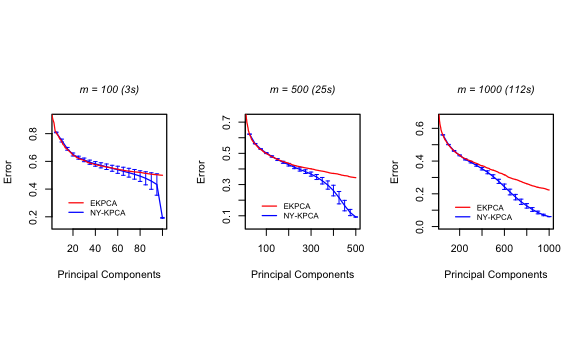
Figure 1: Empirical reconstruction error of EKPCA and average empirical reconstruction error of 100 repetitions of NY-KPCA on digit 5 versus number of principal components $\ell$; error bars represent $\pm 2$ standard deviations. Runtime in seconds is given in parentheses next to the number of Nyström subsamples $m$. Runtime for EKPCA is 337 seconds.

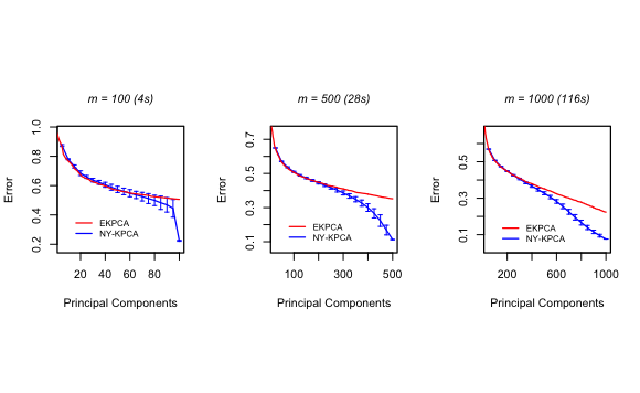
Figure 2: Empirical reconstruction error of EKPCA and average empirical reconstruction error of 100 repetitions of NY-KPCA on digit 5 versus number of principal components $\ell$; error bars represent $\pm 2$ standard deviations. Runtime in seconds is given in parentheses next to the number of Nyström subsamples $m$. Runtime for EKPCA is 478 seconds.

6 Proofs

In this section, we present the proofs.

6.1 Proof of Proposition 3.4

Define

$$Z_{n}:\mathcal{H}\rightarrow\mathbb{R}^{n},\,f\mapsto\left(f(X_{1}),\ldots,f(X_{n})\right)^{\top}\,\,\text{and}\,\,\tilde{Z}_{m}:\mathcal{H}\rightarrow\mathbb{R}^{m},\,f\mapsto\left(f(\tilde{X}_{1}),\ldots,f(\tilde{X}_{n})\right)^{\top}.$$

The adjoint of $\tilde{Z}_{m}$ (Smale and Zhou,, 2007) is given by

$$\tilde{Z}_{m}^{*}:\mathbb{R}^{m}\rightarrow\mathcal{H},\,\alpha\mapsto\sum_{i=1}^{m}\alpha_{i}k(\cdot,\tilde{X}_{i}).$$

Thus, any $f\in\mathcal{H}_{m}$ may be written as $\tilde{Z}_{m}^{*}\alpha$, for some $\alpha\in\mathbb{R}^{m}$ and so

$$\left\langle f,C_{n}f\right\rangle_{\mathcal{H}}=\frac{1}{n}\left\langle\tilde{Z}_{m}^{*}\alpha,Z_{n}^{*}Z_{n}\tilde{Z}_{m}^{*}\alpha\right\rangle_{\mathcal{H}}=\frac{1}{n}\alpha^{\top}\tilde{Z}_{m}Z_{n}^{*}Z_{n}\tilde{Z}_{m}^{*}\alpha,$$

where we used $Z^{*}_{n}Z_{n}=\frac{1}{n}C_{n}$. It is easy to verify that $Z_{n}\tilde{Z}^{*}_{m}=\mathbf{K}_{nm}$ and $\tilde{Z}_{m}Z^{*}_{n}=\mathbf{K}_{mn}$. Therefore, (8) can be written as

$$\arg\sup\left\{\frac{1}{n}\alpha^{\top}\mathbf{K}_{mn}\mathbf{K}_{nm}\alpha:\alpha^{\top}\mathbf{K}_{mm}\alpha=1\right\}.$$ (20)

Letting $\mathbf{u}=\mathbf{K}_{mm}^{1/2}\alpha$ simplifies the constraint in (20) to $\mathbf{u}^{\top}\mathbf{u}=1$, and we write (20) as

$$\arg\sup\left\{\frac{1}{n}\mathbf{u}^{\top}\mathbf{K}_{mm}^{-1/2}\mathbf{K}_{mn}\mathbf{K}_{nm}\mathbf{K}_{mm}^{-1/2}\mathbf{u}:\mathbf{u}^{\top}\mathbf{u}=1\right\}.$$

The solution to the above problem is the unit eigenvector of $\frac{1}{n}\mathbf{K}_{mm}^{-1/2}\mathbf{K}_{mn}\mathbf{K}_{nm}\mathbf{K}_{mm}^{-1/2}$ corresponding to its largest eigenvalue. Denoting this eigenvector as $\mathbf{u}_{1,m}$, we obtain a function $\hat{\phi}_{1,m}\in\mathcal{H}$ solving the NY-KPCA problem in (8) via $\hat{\phi}_{1,m}=\tilde{Z}_{m}^{*}\mathbf{K}_{mm}^{-1/2}\mathbf{u}_{1,m}.$

6.2 Proof of (13)

Note that

$$R(P) {}={} \mathbb{E}\left\lVert(I-P)k(\cdot,X)\right\rVert_{\mathcal{H}}^{2}=\mathbb{E}\left\langle(I-P)k(\cdot,X),(I-P)k(\cdot,X)\right\rangle_{\mathcal{H}}$$ (21)

$${}={} \mathbb{E}\left\langle(I-P)k(\cdot,X),k(\cdot,X)\right\rangle_{\mathcal{H}}=\mathbb{E}\left\langle(I-P),k(\cdot,X)\otimes_{\mathcal{H}}k(\cdot,X)\right\rangle_{\mathcal{L}^{2}(\mathcal{H})},$$

where we used $\left\langle Bf,g\right\rangle_{\mathcal{H}}=\left\langle B,f\otimes_{\mathcal{H}}g\right\rangle_{\mathcal{L}^{2}(\mathcal{H})}$ and $(I-P)^{2}=(I-P)$ in (21). Since $k$ is bounded, it follows that

$$\mathbb{E}\left\langle(I-P),k(\cdot,X)\otimes_{\mathcal{H}}k(\cdot,X)\right\rangle_{\mathcal{L}^{2}(\mathcal{H})}=\left\langle(I-P),\mathbb{E}[k(\cdot,X)\otimes_{\mathcal{H}}k(\cdot,X)]\right\rangle_{\mathcal{L}^{2}(\mathcal{H})}.$$

The result follows by using the above in (21) and noting that

$$\left\langle(I-P),C\right\rangle_{\mathcal{L}^{2}(\mathcal{H})}=\text{tr}\left((I-P)C\right)=\text{tr}\left(C^{1/2}(I-P)(I-P)C^{1/2}\right)$$

$$=\left\langle(I-P)C^{1/2},(I-P)C^{1/2}\right\rangle_{\mathcal{L}^{2}(\mathcal{H})}=\left\lVert(I-P)C^{1/2}\right\rVert_{\mathcal{L}^{2}(\mathcal{H})}^{2},$$

where we have used the invariance of trace under cyclic permutations.

6.3 Proof of Theorem 4.1

$(i)$ For $t>0$, we have

$$R_{C_{n},\ell}^{nys} {}={} \left\lVert(I-P_{m}^{\ell}(C_{n}))C^{1/2}\right\rVert_{\mathcal{L}^{2}(\mathcal{H})}^{2}=\left\lVert(I-P_{m}^{\ell}(C_{n}))(C_{n}+tI)^{1/2}(C_{n}+tI)^{-1/2}C^{1/2}\right\rVert_{\mathcal{L}^{2}(\mathcal{H})}^{2}$$ (22)

$${}\leq{} \left\lVert(I-P_{m}^{\ell}(C_{n}))(C_{n}+tI)^{1/2}\right\rVert_{\mathcal{L}^{\infty}(\mathcal{H})}^{2}\left\lVert(C_{n}+tI)^{-1/2}C^{1/2}\right\rVert_{\mathcal{L}^{2}(\mathcal{H})}^{2}.$$

We now bound the terms in (22). First, we have

$$\left\lVert(C_{n}+tI)^{-1/2}C^{1/2}\right\rVert_{\mathcal{L}^{2}(\mathcal{H})}^{2} {}={} \left\lVert(C_{n}+tI)^{-1/2}(C+tI)^{1/2}(C+tI)^{-1/2}C^{1/2}\right\rVert_{\mathcal{L}^{2}(\mathcal{H})}^{2}$$ (23)

$${}\leq{} \left\lVert(C_{n}+tI)^{-1/2}(C+tI)^{1/2}\right\rVert_{\mathcal{L}^{\infty}(\mathcal{H})}^{2}\left\lVert(C+tI)^{-1/2}C^{1/2}\right\rVert_{\mathcal{L}^{2}(\mathcal{H})}^{2}$$

$${}={} \underbrace{\left\lVert(C_{n}+tI)^{-1/2}(C+tI)^{1/2}\right\rVert_{\mathcal{L}^{\infty}(\mathcal{H})}^{2}}_{(A)}\mathcal{N}_{C}(t),$$

where we used the fact $\left\lVert(C+tI)^{-1/2}C^{1/2}\right\rVert_{\mathcal{L}^{2}(\mathcal{H})}^{2}=\text{tr}(C^{1/2}(C+tI)^{-1}C^{1/2})=\text{tr}((C+tI)^{-1}C)=:\mathcal{N}_{C}(t).$ Next, we have

$$\left\lVert(I-P_{m}^{\ell}(C_{n}))(C_{n}+tI)^{1/2}\right\rVert_{\mathcal{L}^{\infty}(\mathcal{H})}^{2} {}\leq{} 2\underbrace{\left\lVert(I-P_{m})(C_{n}+tI)^{1/2}\right\rVert_{\mathcal{L}^{\infty}(\mathcal{H})}^{2}}_{(B)}$$ (24)

$$\qquad+2\underbrace{\left\lVert(P_{m}-P_{m}^{\ell}(C_{n}))(C_{n}+tI)^{1/2}\right\rVert_{\mathcal{L}^{\infty}(\mathcal{H})}^{2}}_{(D)},$$

where $P_{m}=Z_{m}^{*}(\mathbf{K}_{mm})^{-1}Z_{m}$ is the orthogonal projector onto $\mathcal{H}_{m}$ (see Section 3.2). $(B)$ can be bounded as

$$(B)\leq\underbrace{\left\lVert(I-P_{m})(C+tI)^{1/2}\right\rVert_{\mathcal{L}^{\infty}(\mathcal{H})}^{2}}_{(B_{1})}\underbrace{\left\lVert(C+tI)^{-1/2}(C_{n}+tI)^{1/2}\right\rVert_{\mathcal{L}^{\infty}(\mathcal{H})}^{2}}_{(B_{2})},$$ (25)

and $(D)$ as

$$(D) {}\stackrel{{\scriptstyle(*)}}{{=}}{} \left\lVert(I-P_{m}^{\ell}(C_{n}))P_{m}(C_{n}+tI)^{1/2}\right\rVert_{\mathcal{L}^{\infty}(\mathcal{H})}^{2}$$ (26)

$${}={} \left\lVert(I-P_{m}^{\ell}(C_{n}))P_{m}(C_{n}+tI)P_{m}(I-P_{m}^{\ell}(C_{n}))\right\rVert_{\mathcal{L}^{\infty}(\mathcal{H})}$$

$${}\leq{} \left\lVert(I-P_{m}^{\ell}(C_{n}))P_{m}C_{n}P_{m}(I-P_{m}^{\ell}(C_{n}))\right\rVert_{\mathcal{L}^{\infty}(\mathcal{H})}+t\,\left\lVert(I-P_{m}^{\ell}(C_{n}))P_{m}(I-P_{m}^{\ell}(C_{n}))\right\rVert_{\mathcal{L}^{\infty}(\mathcal{H})},$$

$${}\stackrel{{\scriptstyle(**)}}{{\leq}}{} \hat{\lambda}_{\ell+1,m}+t,$$

where we used the facts that $\mathcal{R}(P_{m}^{\ell}(C_{n}))\subset\mathcal{R}(P_{m})$ in $(*)$ and $P_{m}^{\ell}(C_{n})$ projects onto the $\ell$-eigenspace of $P_{m}C_{n}P_{m}$ in $(**)$. $\hat{\lambda}_{\ell+1,m}$ can be bounded as

$$\hat{\lambda}_{\ell+1,m}\leq|\hat{\lambda}_{\ell+1,m}-\hat{\lambda}_{\ell+1}|+\hat{\lambda}_{\ell+1}\stackrel{{\scriptstyle(\dagger)}}{{\leq}}\frac{1}{n}\left\lVert\tilde{\mathbf{K}}-\mathbf{K}\right\rVert_{{\mathcal{L}^{\infty}(\mathbb{R}^{n})}}+\hat{\lambda}_{\ell},$$ (27)

where $(\dagger)$ follows from the Hoffman-Wiendladt inequality (R. Bhatia,, 1994). We may rewrite (27) as

$$\frac{1}{n}\left\lVert\tilde{\mathbf{K}}-\mathbf{K}\right\rVert_{{\mathcal{L}^{\infty}(\mathbb{R}^{n})}} {}={} \frac{1}{n}\left\lVert Z_{n}(I-P_{m})Z_{n}^{*}\right\rVert_{{\mathcal{L}^{\infty}(\mathbb{R}^{n})}}$$ (28)

$${}={} \left\lVert(I-P_{m})C_{n}(I-P_{m})\right\rVert_{\mathcal{L}^{\infty}(\mathcal{H})}=\left\lVert C_{n}^{1/2}(I-P_{m})C_{n}^{1/2}\right\rVert_{\mathcal{L}^{\infty}(\mathcal{H})}$$

$${}\leq{} \left\lVert C_{n}^{1/2}(C+tI)^{-1/2}\right\rVert_{\mathcal{L}^{\infty}(\mathcal{H})}^{2}\left\lVert(C+tI)^{1/2}(I-P_{m})\right\rVert_{\mathcal{L}^{\infty}(\mathcal{H})}^{2}$$

$${}\stackrel{{\scriptstyle(\ddagger)}}{{\leq}}{} \left\lVert(C_{n}+tI)^{1/2}(C+tI)^{-1/2}\right\rVert_{\mathcal{L}^{\infty}(\mathcal{H})}^{2}\left\lVert(C+tI)^{1/2}(I-P_{m})\right\rVert_{\mathcal{L}^{\infty}(\mathcal{H})}^{2},$$

where we used

$$\left\lVert C_{n}^{1/2}(C+tI)^{-1/2}\right\rVert_{\mathcal{L}^{\infty}(\mathcal{H})}^{2}\leq\left\lVert C_{n}^{1/2}(C_{n}+tI)^{-1/2}\right\rVert_{\mathcal{L}^{\infty}(\mathcal{H})}^{2}\left\lVert(C_{n}+tI)^{1/2}(C+tI)^{-1/2}\right\rVert_{\mathcal{L}^{\infty}(\mathcal{H})}^{2}$$

and $\|C_{n}^{1/2}(C_{n}+tI)^{-1/2}\|_{\mathcal{L}^{\infty}(\mathcal{H})}^{2}\leq 1$ in $(\ddagger)$. The result follows by combining (22)–(28) and employing Lemmas 6.1 and 6.2 for $(iii)$.
$(ii)$ The proof follows exactly as in $(i)$; however, we bound $\left\lVert(I-P_{m})(C+tI)^{1/2}\right\rVert_{\mathcal{L}^{\infty}(\mathcal{H})}^{2}$ with Lemma 6.3 with $t_{0}=\frac{19\kappa}{n}\log\frac{2n}{\delta}$.

Lemma 6.1.

For $\delta>0$, suppose $\frac{9\kappa}{n}\log\frac{n}{\delta}\leq t\leq\lambda_{1}$. Then the following hold:

• $\mathbb{P}^{n}\left\{\sqrt{\frac{2}{3}}\leq\left\lVert(C+tI)^{1/2}(C_{n}+tI)^{-1/2}\right\rVert_{\mathcal{L}^{\infty}(\mathcal{H})}\leq\sqrt{2}\right\}\geq 1-\delta;$

• $\mathbb{P}^{n}\left\{\left\lVert(C+tI)^{-1/2}(C_{n}+tI)^{1/2}\right\rVert_{\mathcal{L}^{\infty}(\mathcal{H})}\leq\sqrt{\frac{3}{2}}\right\}\geq 1-\delta;$

• $\mathbb{P}^{n}\left\{\hat{\lambda}_{\ell}+t\leq\frac{3}{2}(\lambda_{\ell}+t)\right\}\geq 1-\delta.$

Proof.

$(i)$ The result is quoted from Lemma 3.6 of (Rudi et al.,, 2013) with $\alpha=\frac{1}{2}$.

$(ii)$ This is a slight variation of $(i)$ and the proof idea follows that of Lemma 3.6 of (Rudi et al.,, 2013) with $\alpha=\frac{1}{2}$. Note that

$$\left\lVert(C+tI)^{-1/2}(C_{n}+tI)^{1/2}\right\rVert_{\mathcal{L}^{\infty}(\mathcal{H})}=\left\lVert(C+tI)^{-1/2}(C_{n}+tI)(C+tI)^{-1/2}\right\rVert_{\mathcal{L}^{\infty}(\mathcal{H})}^{1/2}.$$

By defining $B_{n}=(C+tI)^{-1/2}(C-C_{n})(C+tI)^{-1/2}$, we have

$$I-B_{n}=(C+tI)^{-1/2}\left((C+tI)-C+C_{n}\right)(C+tI)^{-1/2}=(C+tI)^{-1/2}(C_{n}+tI)(C+tI)^{-1/2}$$

and therefore

$$\left\lVert(C+tI)^{-1/2}(C_{n}+tI)^{1/2}\right\rVert_{\mathcal{L}^{\infty}(\mathcal{H})}=\left\lVert I-B_{n}\right\rVert_{\mathcal{L}^{\infty}(\mathcal{H})}^{1/2}\leq\left(1+\left\lVert B_{n}\right\rVert_{\mathcal{L}^{\infty}(\mathcal{H})}\right)^{1/2}.$$ (29)

It follow from the proof of Lemma 3.6 of (Rudi et al.,, 2013) that for $\frac{9\kappa}{n}\log\frac{n}{\delta}\leq t$,

$$\mathbb{P}^{n}\left\{\left\lVert B_{n}\right\rVert_{\mathcal{L}^{\infty}(\mathcal{H})}\leq\frac{1}{2}\right\}\geq 1-\delta.$$ (30)

Combining (29) and (30) completes the proof.
$(iii)$ Since $\sqrt{\frac{2}{3}}\leq\left\lVert(C+tI)^{1/2}(C_{n}+tI)^{-1/2}\right\rVert_{\mathcal{L}^{\infty}(\mathcal{H})}$ as obtained in $(i)$, it is equivalent (see (Rudi et al.,, 2013, Lemmas B.2 and 3.5)) to $C_{n}+tI\preceq\frac{3}{2}(C+tI)$. This implies (see Gohberg et al.,, 2003) that $\lambda_{k}(C_{n}+tI)\leq\lambda_{k}(\frac{3}{2}(C+tI))=\frac{3}{2}\lambda_{k}(C+tI)$ for all $k\geq 1$. ∎

Lemma 6.2 ((Rudi et al.,, 2015), Lemma 6).

Suppose Assumption 3.1 holds, and suppose for some $m<n$, the set $\{\tilde{X}_{j}\}_{j=1}^{m}$ is drawn uniformly from the set of all partitions of size $m$ of the training data, $\{X_{i}\}_{i=1}^{n}$. For $t>0$ and any $\delta>0$ such that $m\geq\left(67\vee 5\mathcal{N}_{C,\infty}(t)\right)\log\frac{4\kappa}{t\delta}$, we have

$$\mathbb{P}^{n}\left\{\left\lVert(I-P_{m})(C+tI)^{1/2}\right\rVert_{\mathcal{L}^{\infty}(\mathcal{H})}^{2}\leq 3t\right\}\geq 1-\delta,$$

where $P_{m}$ is the orthogonal projector onto $\mathcal{H}_{m}=\emph{span}\{k(\cdot,\tilde{X}_{j})|j\in[m]\}$.

Lemma 6.3 ((Rudi et al.,, 2015), Lemma 7).

Suppose Assumption 3.1 holds. Let $(\hat{l}_{i}(s))_{i=1}^{n}$ be the collection of approximate leverage scores. Letting $N:=\{1,...,n\}$, for $t>0$ define $p_{t}$ as the distribution over $N$ with probabilities $p_{t}(i)=\hat{l}_{i}(t)/\sum_{j=1}^{n}\hat{l}_{j}(t)$. Let $\mathcal{I}_{m}=\{i_{1},...,i_{m}\}\subset N$ be a collection of indices independently sampled from $p_{t}$ with replacement. Let $P_{m}$ be the orthogonal projector onto $\mathcal{H}_{m}=\emph{span}\{k(\cdot,\tilde{X}_{j})|j\in\mathcal{I}_{m}\}$. Additionally, for any $\delta>0$, suppose the following hold:

1. There exists $T\geq 1$ and $t_{0}>0$ such that for any $s\geq t_{0}$, $(\hat{l}_{i}(s))_{i=1}^{n}$ are $T-$approximate leverage scores with confidence $\delta$,

2. $n\geq 1655\kappa+223\kappa\log\frac{2\kappa}{\delta},$

3. $t_{0}\vee\frac{19\kappa}{n}\log\frac{2n}{\delta}\leq t\leq\lambda_{1},$

4. $m\geq 334\log\frac{8n}{\delta}\vee 78T^{2}\mathcal{N}_{C}(t)\log\frac{8n}{\delta}$.

Then

$$\mathbb{P}^{n}\left\{\left\lVert(I-P_{m})(C+tI)^{1/2}\right\rVert_{\mathcal{L}^{\infty}(\mathcal{H})}^{2}\leq 3t\right\}\geq 1-2\delta.$$

6.4 Proof of Corollary 4.2

$(i)$ From Theorem 4.1 $(i)$ we have

$$R_{C,\ell}=\sum_{i>\ell}\lambda_{i}\lesssim\sum_{i>\ell}i^{-\alpha}\lesssim\int_{\ell}^{\infty}x^{-\alpha}dx\lesssim\ell^{1-\alpha}=n^{-\theta(1-\frac{1}{\alpha})}.$$

Similarly,

$$R_{C,\ell}=\sum_{i>\ell}\lambda_{i}\gtrsim\sum_{i>\ell}i^{-\alpha}\gtrsim\int_{\ell}^{\infty}x^{-\alpha}dx\gtrsim\ell^{1-\alpha}=n^{-\theta(1-\frac{1}{\alpha})}.$$

$(ii)$ This is Theorem 3.2 of (Rudi et al.,, 2015) with $\alpha=\frac{1}{2}$, $r=\alpha$, $p=2$, and $\ell=n^{\frac{\theta}{\alpha}}$.
$(iii)$ Theorem 4.1 $(iii)$ and Proposition A.1 yield

$$R_{C_{n},\ell}^{nys}\lesssim_{\mathbb{P}^{n}}t^{-\frac{1}{\alpha}}n^{-\theta}+t^{1-\frac{1}{\alpha}}\leq\begin{cases}t^{1-\frac{1}{\alpha}},\qquad\quad\hskip 2.84526ptt\geq n^{-\theta}\\ t^{-\frac{1}{\alpha}}n^{-\theta},\qquad t\leq n^{-\theta}\end{cases},$$

where $\frac{\log n}{n}\lesssim t\leq\lambda_{1}$ and $m\gtrsim\mathcal{N}_{C,\infty}(t)\log\frac{1}{t}$ with $\mathcal{N}_{C,\infty}(t)=\sup_{x\in\mathcal{X}}\left\langle k(\cdot,x),(C+tI)^{-1}k(\cdot,x)\right\rangle_{\mathcal{H}}\lesssim\frac{1}{t}$. First, consider the case when $t\geq n^{-\theta}$. This means

$$R_{C_{n},\ell}^{nys}\lesssim\inf\left\{t^{1-\frac{1}{\alpha}}:t\gtrsim\frac{\log n}{n}\vee n^{-\theta},m\gtrsim\frac{1}{t}\log\frac{1}{t}\right\}.$$

For $\theta<1$, we obtain

$$R_{C_{n},\ell}^{nys}\lesssim\inf\left\{t^{1-\frac{1}{\alpha}}:t\gtrsim n^{-\theta},m\gtrsim\frac{1}{t}\log\frac{1}{t}\right\}\leq n^{-\theta\left(1-\frac{1}{\alpha}\right)}$$

if $m\gtrsim n^{\theta}\log n$. For $\theta\geq 1$, we obtain

$$R_{C_{n},\ell}^{nys}\lesssim\inf\left\{t^{1-\frac{1}{\alpha}}:t\gtrsim\frac{\log n}{n},m\gtrsim\frac{1}{t}\log\frac{1}{t}\right\}\leq\left(\frac{\log n}{n}\right)^{\left(1-\frac{1}{\alpha}\right)}$$

if $m\gtrsim\frac{n}{\log n}\log\frac{n}{\log n}$. Next, consider the case when $t\leq n^{-\theta}$ which means

$$R_{C_{n},\ell}^{nys}\lesssim\inf\left\{t^{-\frac{1}{\alpha}}n^{-\theta}:\frac{\log n}{n}\lesssim t\lesssim n^{-\theta},m\gtrsim\frac{1}{t}\log\frac{1}{t}\right\}\leq n^{-\theta\left(1-\frac{1}{\alpha}\right)}$$

when $\theta<1$ and $m\gtrsim n^{\theta}\log n$.
$(iv)$ Theorem 4.1$(iv)$ and Proposition A.1 yield

$$R_{C_{n},\ell}^{nys}\lesssim_{\mathbb{P}^{n}}t^{-\frac{1}{\alpha}}n^{-\theta}+t^{1-\frac{1}{\alpha}}\leq\begin{cases}t^{1-\frac{1}{\alpha}},\qquad\quad\hskip 2.84526ptt\geq n^{-\theta}\\ t^{-\frac{1}{\alpha}}n^{-\theta},\qquad t\leq n^{-\theta}\end{cases},$$

where $\frac{\log n}{n}\lesssim t\leq\lambda_{1}$ and $m\gtrsim\mathcal{N}_{C}(t)\log n\gtrsim t^{-\frac{1}{\alpha}}\log n$. The result follows by carrying out the analysis as in $(iii)$ for $\theta<1$ and $\theta\geq 1$.

6.5 Proof of Corollary 4.3

$(i)$ From Theorem 4.1 $(i)$ we have

$$R_{C,\ell}=\sum_{i>\ell}\lambda_{i}\lesssim\sum_{i>\ell}e^{-\tau i}\lesssim\int_{\ell}^{\infty}e^{-\tau x}dx\lesssim e^{-\tau\ell}=n^{-\theta}$$

and

$$R_{C,\ell}=\sum_{i>\ell}\lambda_{i}\gtrsim\sum_{i>\ell}e^{-\tau i}\gtrsim\int_{\ell+1}^{\infty}e^{-\tau x}dx\gtrsim e^{-\tau(\ell+1)}=e^{-\tau}n^{-\theta}.$$

$(ii)$ Theorem 4.1 $(ii)$ and Proposition A.2 yield

$$R_{C_{n},\ell}\lesssim_{\mathbb{P}^{n}}\left(n^{-\theta}+t\right)\log\frac{1}{t}\leq\begin{cases}n^{-\theta}\log\frac{1}{t},\qquad\hskip 2.84526ptt\leq n^{-\theta}\\ t\log\frac{1}{t},\qquad\quad\hskip 5.69054ptt\geq n^{-\theta}\end{cases},$$

where $\frac{\log n}{n}\lesssim t\leq\lambda_{1}$. For the case of $t\leq n^{-\theta}$, we obtain

$$R_{C_{n},\ell}\lesssim\inf\left\{n^{-\theta}\log\frac{1}{t}:\frac{\log n}{n}\lesssim t\leq n^{-\theta}\right\}=n^{-\theta}\log n,$$

where the constraint is only valid for $\theta<1$. On the other hand, for $t\geq n^{-\theta}$, we obtain

$$R_{C_{n},\ell}\lesssim\inf\left\{t\log\frac{1}{t}:t\gtrsim\frac{\log n}{n}\vee n^{-\theta}\right\}=\frac{\log n}{n}\log\left(\frac{n}{\log n}\right)\leq\frac{(\log n)^{2}}{n},$$

which holds for $\theta\geq 1$.
$(iii)$ Arguing similarly as in $(ii)$, it follows that for $\theta<1$ and $m\gtrsim n^{\theta}\log n$, we obtain a rate of $n^{-\theta}\log n$ for $R^{nys}_{C_{n},\ell}$. Similarly for $\theta\geq 1$ and $m\geq\frac{n}{\log n}\log\left(\frac{n}{\log n}\right)$, we obtain a rate of $n^{-1}(\log n)^{2}$.
$(iv)$ Arguing as in $(ii)$ and enforcing the restriction $m\gtrsim\log n\log\frac{1}{t}$ imposed by Theorem 4.1 $(ii)$ yields the result.

7 Conclusions

In this paper, we considered the problem of deriving an approximation to kernel PCA using Nyström method. This latter approach seemingly overcomes some of the difficulties of other approaches based on random features. In particular, it allows to derive error estimates directly comparable to those typically considered to analyze the statistical properties of KPCA. Our results indicate the existence of regimes where computational gains can be achieved while preserving statistical accuracy. These results parallel recent findings in supervised learning and are among the first of this kind for unsupervised learning.

Our study opens a number of possible questions. For example, still for KPCA, it would be interesting to understand the properties of Nyström sampling in combination with iterative eigensolvers, both batch (e.g., the power method) and stochastic (e.g., Oja’s rule). The application of our approach to other spectral methods, such as those used in graph and manifold learning, would be interesting. Beyond PCA and spectral methods, our study naturally yields the question of which other learning problems can have analogous statistical and computational trade-offs. For example, it would be interesting to consider applications of our approach to independence tests based on covariance and cross-covariance operators (Gretton et al.,, 2008), or mean embeddings (Sriperumbudur et al.,, 2010).

Appendix A Technical Results

Proposition A.1.

Suppose $\underline{A}i^{-\alpha}\leq\lambda_{i}\leq\bar{A}i^{-\alpha}$ for $\alpha>1$ and $\underline{A},\bar{A}\in(0,\infty)$. The following holds:

$$\mathcal{N}_{C}(t)\lesssim t^{-1/\alpha}.$$

Proof.

We have

$$\mathcal{N}_{C}(t)=\text{tr}\left((C+tI)^{-1}C\right)=\sum_{i\geq 1}\frac{\lambda_{i}}{\lambda_{i}+t}\leq\sum_{i\geq 1}\frac{\bar{A}i^{-\alpha}}{\underline{A}i^{-\alpha}+t}=\frac{\bar{A}}{\underline{A}}\sum_{i\geq 1}\frac{i^{-\alpha}}{i^{-\alpha}+t\underline{A}^{-1}}.$$

Let $u=t^{1/\alpha}\underline{A}^{-1/\alpha}x\implies u^{\alpha}=t\underline{A}^{-1}x^{\alpha}$ and $dx=t^{-1/\alpha}\underline{A}^{1/\alpha}du$. Therefore,

$$\sum_{i\geq 1}\frac{i^{-\alpha}}{i^{-\alpha}+t\underline{A}^{-1}}\leq\int_{0}^{\infty}\frac{x^{-\alpha}}{x^{-\alpha}+t\underline{A}^{-1}}\,dx=\int_{0}^{\infty}\frac{1}{1+t\underline{A}^{-1}x^{\alpha}}dx=\left(\frac{\underline{A}}{t}\right)^{1/\alpha}\int_{0}^{\infty}\frac{1}{1+u^{\alpha}}du.$$

Since $\frac{1}{1+u^{\alpha}}$ is decreasing in $\alpha$ on $u\in(0,\infty)$, we have

$$\frac{1}{1+u^{\alpha}}\leq\frac{1}{1+u^{2}},\hskip 8.53581pt\text{if}\hskip 8.53581pt\alpha\geq 2.$$

So for $2\leq\alpha$,

$$\left(\frac{\underline{A}}{t}\right)^{1/\alpha}\int_{0}^{\infty}\frac{1}{1+u^{\alpha}}du\stackrel{{\scriptstyle<}}{{\sim}}t^{-1/\alpha}\int_{0}^{\infty}\frac{1}{1+u^{2}}du=t^{-1/\alpha}\,\left[\tan^{-1}(u)|_{0}^{\infty}\right]=\frac{\pi}{2}t^{-1/\alpha},$$

implying $\mathcal{N}_{C}(t)\lesssim t^{-1/\alpha}$. For $1<\alpha<2$, we obtain

$$t^{-1/\alpha}\int_{0}^{\infty}\frac{1}{1+u^{\alpha}}du\leq t^{-1/\alpha}\sum_{k=0}^{\infty}\frac{1}{1+k^{\alpha}}\leq t^{-1/\alpha}\left(1+\sum_{k=1}^{\infty}\frac{1}{k^{\alpha}}\right).$$

Since $1+\sum_{k=1}^{\infty}\frac{1}{k^{\alpha}}$ converges for $\alpha>1$, we obtain $\mathcal{N}_{C}(t)\lesssim t^{-1/\alpha}.$ ∎

Proposition A.2.

Suppose $\underline{B}e^{-\tau i}\leq\lambda_{i}\leq\bar{B}e^{-\tau i}$ for $\tau>0$ and $\underline{B},\bar{B}\in(0,\infty)$. Let $\ell=\frac{1}{\tau}\log n^{\theta}$, $\theta>0$. Then

$$\mathcal{N}_{C}(t)\lesssim\log\left(\frac{1}{t}\right).$$

Proof.

We have

$$\mathcal{N}_{C}(t)=\text{tr}\left((C+tI)^{-1}C\right)=\sum_{i\geq 1}\frac{\lambda_{i}}{\lambda_{i}+t}\leq\frac{\bar{B}e^{-\tau i}}{\underline{B}e^{-\tau i}+t}=\frac{\bar{B}}{\underline{B}}\sum_{i\geq 1}\frac{1}{1+t\underline{B}^{-1}e^{\tau i}}$$

$$\lesssim\int_{0}^{\infty}\frac{1}{1+t\underline{B}^{-1}e^{\tau x}}dx=\left[x-\frac{1}{\tau}\log\left(t\underline{B}^{-1}\,e^{\tau x}+1\right)\right]\Big{|}_{0}^{\infty}.$$

Since

$$x-\frac{1}{\tau}\log\left(t\underline{B}^{-1}\,e^{\tau x}+1\right)=\frac{1}{\tau}\left(\log(e^{\tau x})-\log\left(t\underline{B}^{-1}\,e^{\tau x}+1\right)\right)=\frac{1}{\tau}\log\left(t^{-1}\underline{B}\frac{e^{\tau x}}{\,e^{\tau x}+t^{-1}\underline{B}}\right),$$

evaluating

$$\frac{1}{\tau}\log\left(t^{-1}\underline{B}\frac{e^{\tau x}}{\,e^{\tau x}+t^{-1}\underline{B}}\right)\Big{|}_{0}^{\infty}$$

yields the result. ∎

References

- Alaoui and Mahoney, (2015) Alaoui, A. and Mahoney, M. (2015). Fast randomized kernel ridge regression with statistical guarantees. In Cortes, C., Lawrence, N. D., Lee, D. D., Sugiyama, M., and Garnett, R., editors, Advances in Neural Information Processing Systems 28, pages 775–783. Curran Associates, Inc.
- Alaoui and Mahoney, (2014) Alaoui, A. and Mahoney, M. W. (2014). Fast Randomized Kernel Methods With Statistical Guarantees. arXiv.
- Bach, (2013) Bach, F. (2013). Sharp analysis of low-rank kernel matrix approximations. In Shalev-Shwartz, S. and Steinwart, I., editors, Proc. of the 26th Annual Conference on Learning Theory, volume 30 of Proceedings of Machine Learning Research, pages 185–209. PMLR.
- Blanchard et al., (2007) Blanchard, G., Bousquet, O., and Zwald, L. (2007). Statistical properties of kernel principal component analysis. Machine Learning, 66(2):259–294.
- Bottou and Bousquet, (2008) Bottou, L. and Bousquet, O. (2008). The tradeoffs of large scale learning. In Platt, J., Koller, D., Singer, Y., and Roweis, S., editors, Advances in Neural Information Processing Systems, volume 20, pages 161–168. Curran Associates, Inc.
- Calandriello et al., (2018) Calandriello, D., Lazaric, A., and Valko, M. (2018). Distributed adaptive sampling for kernel matrix approximation. CoRR, abs/1803.10172.
- Cohen et al., (2015) Cohen, M. B., lee, Y. T., Musco, C., Musco, C., Peng, R., and Sidford, A. (2015). Uniform sampling for matrix approximation. In Proceedings of the 2015 Conference on Innovations in Theoretical Computer Science, pages 181–190. ACM.
- Drineas et al., (2012) Drineas, P., Magdon-Ismail, M., Mahoney, M. W., and Woodruff, D. P. (2012). Fast approximation of matrix coherence and statistical leverage. Journal of Machine Learning Research, 13:3475–3506.
- Drineas and Mahoney, (2005) Drineas, P. and Mahoney, M. W. (2005). On the Nyström method for approximating a Gram matrix for improved kernel-based learning. Journal of Machine Learning Research, 6:2153–2175.
- Gittens and Mahoney, (2013) Gittens, A. and Mahoney, M. (2013). Revisiting the Nyström method for improved large-scale machine learning. In Dasgupta, S. and McAllester, D., editors, Proc. of the 30th International Conference on Machine Learning, volume 28 of Proceedings of Machine Learning Research, pages 567–575. PMLR.
- Gohberg et al., (2003) Gohberg, I., Goldberg, S., and Kaashoek, R. (2003). Basic Classes of Linear Operators. Birkhauser, Basel, Switzerland.
- Gretton et al., (2008) Gretton, A., Fukumizu, K., Teo, C.-H., Song, L., Schölkopf, B., and Smola, A. (2008). A kernel statistical test of independence. In Advances in Neural Information Processing Systems 20, pages 585–592. MIT Press.
- Jin et al., (2013) Jin, R., Yang, T., Mahdavi, M., Li, Y.-F., and Zhou, Z.-H. (2013). Improved bounds for the Nyström method with application to kernel classification. IEEE Transactions on Information Theory, 59(10):6939–6949.
- Jolliffe, (1986) Jolliffe, I. (1986). Principal Component Analysis. Springer-Verlag, New York, USA.
- Kimeldorf and Wahba, (1971) Kimeldorf, G. S. and Wahba, G. (1971). Some results on Tchebycheffian spline functions. Journal of Mathematical Analysis and Applications, 33:82–95.
- Musco and Musco, (2017) Musco, C. and Musco, C. (2017). Recursive sampling for the nyström method. In Guyon, I., Luxburg, U. V., Bengio, S., Wallach, H., Fergus, R., Vishwanathan, S., and Garnett, R., editors, Advances in Neural Information Processing Systems 30, pages 3833–3845. Curran Associates, Inc.
- Orabona et al., (2008) Orabona, F., Keshet, J., and Caputo, B. (2008). The projectron: a bounded kernel-based perceptron. In Cohen, W. W., McCallum, A., and Roweis, S. T., editors, ICML, volume 307 of ACM International Conference Proceeding Series, pages 720–727. ACM.
- R. Bhatia, (1994) R. Bhatia, L. E. (1994). The Hoffman-Wielandt inequality in infinite dimensions. In Proceedings of the Indian Academy of Sciences - Mathematical Sciences, volume 104, pages 483–494.
- Rahimi and Recht, (2008) Rahimi, A. and Recht, B. (2008). Random features for large-scale kernel machines. In Platt, J. C., Koller, D., Singer, Y., and Roweis, S. T., editors, Advances in Neural Information Processing Systems 20, pages 1177–1184. Curran Associates, Inc.
- Reed and Simon, (1980) Reed, M. and Simon, B. (1980). Methods of Modern Mathematical Physics: Functional Analysis I. Academic Press, New York.
- Rudi et al., (2015) Rudi, A., Camoriano, R., and Rosasco, L. (2015). Less is more: Nyström computational regularization. In Cortes, C., Lawrence, N. D., Lee, D. D., Sugiyama, M., and Garnett, R., editors, Advances in Neural Information Processing Systems 28, pages 1657–1665. Curran Associates, Inc.
- Rudi et al., (2013) Rudi, A., Canas, G. D., and Rosasco, L. (2013). On the sample complexity of subspace learning. In Advances in Neural Information Processing Systems 26, pages 2067–2075.
- Rudi and Rosasco, (2017) Rudi, A. and Rosasco, L. (2017). Generalization properties of learning with random features. In Guyon, I., Luxburg, U. V., Bengio, S., Wallach, H., Fergus, R., Vishwanathan, S., and Garnett, R., editors, Advances in Neural Information Processing Systems 30, pages 3215–3225. Curran Associates, Inc.
- Schölkopf et al., (2001) Schölkopf, B., Herbrich, R., and Smola, A. (2001). A generalized representer theorem. In Proc. of the 14th Annual Conference on Computational Learning Theory and 5th European Conference on Computational Learning Theory, pages 416–426, London, UK. Springer-Verlag.
- Schölkopf et al., (1998) Schölkopf, B., Smola, A., and Müller, K.-R. (1998). Nonlinear component analysis as a kernel eigenvalue problem. Neural Computation, 10:1299–1319.
- Shawe-Taylor et al., (2005) Shawe-Taylor, J., Williams, C., Christianini, N., and Kandola, J. (2005). On the eigenspectrum of the Gram matrix and the generalisation error of kernel PCA. EEE Transactions on Information Theory, 51(7):2510–2522.
- Smale and Zhou, (2007) Smale, S. and Zhou, D.-X. (2007). Learning theory estimates via integral operators and their approximations. Constructive Approximation, 26:153–172.
- Sriperumbudur et al., (2010) Sriperumbudur, B. K., Gretton, A., Fukumizu, K., Schölkopf, B., and Lanckriet, G. R. G. (2010). Hilbert space embeddings and metrics on probability measures. Journal of Machine Learning Research, 11:1517–1561.
- Sriperumbudur and Sterge, (2018) Sriperumbudur, B. K. and Sterge, N. (2018). Approximate kernel PCA using random features: Computational vs. statistical trade-off. arXiv.
- Ullah et al., (2018) Ullah, M. E., Mianjy, P., Marinov, T. V., and Arora, R. (2018). Streaming kernel PCA with random features. In Bengio, S., Wallach, H., Larochelle, H., Grauman, K., Cesa-Bianchi, N., and Garnett, R., editors, Advances in Neural Information Processing Systems 31, pages 7322–7332. Curran Associates, Inc.
- Williams and Seeger, (2001) Williams, C. and Seeger, M. (2001). Using the Nyström method to speed up kernel machines. In T. K. Leen, T. G. Diettrich, V. T., editor, Advances in Neural Information Processing Systems 13, pages 682–688, Cambridge, MA. MIT Press.