Continued fractions and Hankel determinants from hyperelliptic curves

Abstract

Following van der Poorten, we consider a family of nonlinear maps which are generated from the continued fraction expansion of a function on a hyperelliptic curve of genus $\mathrm{g}$. Using the connection with the classical theory of J-fractions and orthogonal polynomials, we show that in the simplest case $\mathrm{g}=1$ this provides a straightforward derivation of Hankel determinant formulae for the terms of a general Somos-4 sequence, which were found in a particular form by Chang, Hu and Xin, We extend these formulae to the higher genus case, and prove that generic Hankel determinants in genus two satisfy a Somos-8 relation. Moreover, for all $\mathrm{g}$ we show that the iteration for the continued fraction expansion is equivalent to a discrete Lax pair with a natural Poisson structure, and the associated nonlinear map is a discrete integrable system.

Dedicated to the memory of Jon Nimmo.

Keywords: J-fraction, hyperelliptic curve, Hankel determininant, Somos sequence.

1 Introduction

The Somos-4 recurrence is given by

$$\tau_{n+4}\tau_{n}=\alpha\,\tau_{n+3}\tau_{n+1}+\beta\,\tau_{n+2}^{2}.$$ (1.1)

The surprising observation of Somos was that when ${\alpha}={\beta}=1$ and the four initial values $\tau_{0},\tau_{1},\tau_{2},\tau_{3}$ are all 1, the recurrence (1.1) generates a sequence of integers [49], beginning with

$$1,1,1,1,2,3,7,23,59,314,1529,8209,83313,620297,\ldots.$$ (1.2)

A proof of this fact was eventually published [36], but a better understanding of the mechanism by which such rational recurrences can yield integer sequences came from the observation that (1.1) exhibits the Laurent property [21]: the iterates are Laurent polynomials in the initial values with integer coefficients, that is to say

$$\tau_{n}\in{\mathbb{Z}}[\tau_{0}^{\pm 1},\tau_{1}^{\pm 1},\tau_{2}^{\pm 1},\tau_{3}^{\pm 1},{\alpha},{\beta}]$$

for all $n$, which makes it obvious why (1.2) consists entirely of integers. The Laurent phenomenon [19] eventually appeared as a key property of the distinguished generators (cluster variables) in Fomin and Zelevinsky’s cluster algebras [18], which are constructed by a recursive process called mutation, and Fordy and Marsh showed how the Somos-4 recurrence and various higher order analogues arise from cluster mutations starting from quivers of a particular type [20].

Cluster algebras fit within a broader setting of Laurent phenomenon algebras [33], leading to a wide variety of nonlinear recurrences that exhibit the Laurent property [2]; and it is possible to reverse engineer a rational recurrence to generate an integer sequence [15]. However, Somos-4 sequences have some very special features which are a consequence of the fact that each such sequence is associated with a sequence of points $P_{0}+nP$ on an elliptic curve $E$, and this leads to an analytic formula for the terms of the sequence. The following result was proved in [23].

Theorem 1.1.

The terms of a Somos-4 sequence, generated by (1.1) from four non-zero initial values $\tau_{0},\tau_{1},\tau_{2},\tau_{3}$, non-zero ${\alpha}$ and arbitrary ${\beta}\in{\mathbb{C}}$, are given by

$$\tau_{n}=\hat{a}\hat{b}^{n}\,\frac{{\sigma}(z_{0}+nz)}{{\sigma}(z)^{n^{2}}},$$ (1.3)

where ${\sigma}(z)={\sigma}(z;g_{2},g_{3})$ is the Weierstrass sigma function associated with the elliptic curve $E:\,y^{2}=4x^{3}-g_{2}x-g_{3}$ over ${\mathbb{C}}$ with period lattice $\Lambda$, with $z_{0}=\int_{\infty}^{P_{0}}\frac{\mathrm{d}x}{y}$, $z=\int_{\infty}^{P}\frac{\mathrm{d}x}{y}\in{\mathbb{C}}\bmod\Lambda$ corresponding to points $P_{0},P\in E$, and $\hat{a},\hat{b}$ are certain non-zero constants.

The formula (1.3) also makes sense in the degenerate case when the discriminant $g_{2}^{3}-27g_{3}^{2}=0$. Although the above result is formulated over the complex numbers, its algebraic content - associating a solution of (1.1) with a sequence of points on an elliptic curve - is valid in any field over which the initial values and coefficients ${\alpha},{\beta}$ are defined (up to appropriate adjustments in characteristic 2 or 3); this was described independently by Swart [51], and also, in terms of a quartic model for $E$, by van der Poorten [43]. This underlying algebraic structure has many consequences, including the existence of higher order relations between the terms [24, 34, 44], and more refined versions of the Laurent property which produce large families of integer sequences [25]. From this point of view, Somos-4 sequences are natural extensions of Ward’s elliptic divisibility sequences [55], which correspond to the special case $P_{0}=\infty$ (the identity element in the group law of $E$), and generalize the arithmetical properties of Fibonacci or Lucas sequences to a nonlinear setting [16]. Aside from their intrinsic interest for certain problems of an arithmetical [48] or Diophantine nature [9], Somos sequences and their higher order analogues appear in discrete integrable systems, underlying many integrable maps [28], especially via reductions of the discrete Hirota equation (bilinear discrete KP, also known as the octahedron recurrence) [27] or Miwa’s equation (bilinear discrete BKP, or the cube recurrence) [17]. They also arise in solvable models of statistical mechanics and quantum field theory, such as the hard hexagon model, as mentioned in [47], or dimer models and quiver gauge theory [14].

It was conjectured by Somos, and later proved by Xin [56], that the terms of the sequence (1.2) have another explicit expression that is rather different from (1.3), being given by the Hankel determinants

$$D_{n}=\det(\tilde{s}_{i+j-2})_{i,j=1,\ldots,n},$$ (1.4)

where the entries $\tilde{s}_{j}$ are obtained from the function $\eta=\eta(x)$ satisfying the algebraic equation

$$\eta-\eta^{2}=x-x^{3}.$$ (1.5)

To be precise, solving (1.5) for $\eta$ with a fixed choice of square root, one should take the function $\tilde{G}=\eta/x-1$, and expand it as

$$\frac{\eta}{x}-1=\sum_{j\geq 1}\tilde{s}_{j-1}x^{j}=x+x^{2}+3x^{3}+8x^{4}+23x^{5}+\cdots,$$ (1.6)

which gives

$$D_{0}=D_{1}=1,\qquad D_{2}=\left|\begin{array}[]{cc}1&1\\ 1&3\end{array}\right|=2,\quad D_{3}=\left|\begin{array}[]{ccc}1&1&3\\ 1&3&8\\ 3&8&23\end{array}\right|=3,$$ (1.7)

and so on, where the matrix entries are generated by the recursion

$$\tilde{s}_{j}=\tilde{{\alpha}}\tilde{s}_{j-1}+\tilde{{\beta}}\tilde{s}_{j-2}+\tilde{{\gamma}}\sum_{i=0}^{j-2}\tilde{s}_{i}\tilde{s}_{j-2-i},\qquad j\geq 2,$$ (1.8)

with $\tilde{\alpha}=2$, $\tilde{{\beta}}=0$, $\tilde{{\gamma}}=1$ and $\tilde{s}_{0}=\tilde{s}_{1}=1$. It was further conjectured by Barry [4] that the Hankel determinants $D_{n}$ formed from a particular family of sequences $(\tilde{s}_{j})$, defined by the recursion (1.8) with $\tilde{s}_{0}=1$, $\tilde{s}_{1}=\tilde{{\alpha}}$, satisfy the Somos-4 recurrence (1.1) with coefficients ${\alpha}=\tilde{{\alpha}}^{2}\tilde{{\gamma}}^{2}$, ${\beta}=\tilde{{\gamma}}^{2}(\tilde{{\beta}}+\tilde{{\gamma}})^{2}-\tilde{{\alpha}}^{2}\tilde{{\gamma}}^{3}$, and this was proved by Chang and Hu using identities for block Hankel determinants [10]. The latter result does not overlap with that of Xin, since the conditions on the coefficients and initial conditions do not include the original sequence (1.2). However, it was subsequently shown by Chang, Hu and Xin that, for any Somos-4 sequence with two adjacent initial values equal to 1, the terms with positive index $n$ are given by a Hankel determinant of the form (1.4), where the entries $\tilde{s}_{j}$ satisfy a recursion of the form (1.8), for a suitable choice of $\tilde{\alpha},\tilde{{\beta}},\tilde{{\gamma}},\tilde{s}_{0},\tilde{s}_{1}$ [11].

In this paper we start from van der Poorten’s construction in [43] for Somos-4, based on the continued fraction expansion of a function on a quartic curve of genus one, and the results of [45, 46]. In the latter work, the continued fraction approach was extended to hyperelliptic curves of higher genus $\mathrm{g}$, defined by a polynomial of even degree $2\mathrm{g}+2$, but with partial success: a Somos-6 relation was obtained in genus two, but only in a special case. The continued fraction expansion of a hyperelliptic function of a certain type is described in section 2 (for other related results, and the connection with the geometry of the Jacobian of the curve, see [1, 5, 6, 22, 42]). Next, in section 3, the recursion for the continued fraction is reformulated as a discrete dynamical system defined by a matrix linear problem (a discrete Lax pair), and we state the first main result, Theorem 3.1, which says that this nonlinear dynamical system is integrable in the sense that it satisfies a discrete analogue of the Liouville-Arnold theorem from classical mechanics [3], having an invariant symplectic structure and a sufficient number of first integrals in involution with respect to the corresponding Poisson bracket (see [8, 35, 53] for the precise definition of a discrete integrable system). We present explicit details of the symplectic map and first integrals for the cases $\mathrm{g}=1$ and $\mathrm{g}=2$, while the complete proof for any $\mathrm{g}$ is deferred until section 6.

Section 4 is concerned with the derivation of Hankel determinant formulae for the solutions of the nonlinear system, based on the classical theory of J-fractions and orthogonal polynomials, which are presented in a uniform fashion for any genus $\mathrm{g}$. (Note that Hankel determinants and continued fractions have appeared in the solution of many other integrable systems, particularly those of Toda type, and Painlevé equations [12, 31, 50], and there are more recent results in the broader context of Padé approximants associated with isomonodromic deformations [37].) Subsequently, in section 5, we show how the Hankel formulae obtained generalize the results of Chang, Hu and Xin on Somos-4 sequences: even in the elliptic case $\mathrm{g}=1$, the results are more general than [11], since the Hankel determinants depend on an additional free parameter, and the formulae from the previous section extend to negative indices $n$. In genus two we prove that, for generic parameter values, the corresponding Hankel determinants satisfy a Somos-8 relation (Theorem 5.4), and indicate how van der Poorten’s Somos-6 recurrence arises as a special case. We also present a precise conjecture that provides an analytic formula analogous to (1.3) for the Hankel determinants in genus two, and briefly explain how an appropriate higher genus analogue of this conjecture implies the existence of Somos recurrences for all values of $\mathrm{g}$.

In section 6 we employ a space of $2\times 2$ Lax matrices, related to those in section 3 by a gauge transformation, which admits a natural Poisson structure, and construct a completely integrable system on this phase space, given by a set of commuting flows defined by suitable Hamiltonian functions. We then show how the nonlinear map coming from the continued fraction arises from a Poisson map on this phase space, which preserves the same Hamiltonians and Casimirs as the continuous system. The map we obtain is somewhat reminiscent of the Bäcklund transformation (BT) for the even Mumford systems, introduced in [32], except that the entries of the Lax pair have a different degree structure, and (in contast with the BT, which is a multivalued correspondence) it is an explicit birational map. Some determinantal identities that directly yield the formulae for the coefficients of J-fractions are also presented in an appendix.

2 Continued fractions for hyperelliptic functions

Following van der Poorten [43, 45, 46], we consider a hyperelliptic curve defined by

$${\cal C}:\qquad Y^{2}=F(X),$$ (2.1)

where

$$F(X)=A(X)^{2}+4R(X)$$ (2.2)

for a pair of polynomials

$$A(X)=X^{\mathrm{g}+1}+\cdots,\qquad R(X)=u\,X^{\mathrm{g}}+\cdots.$$

In addition to the affine points $(X,Y)\in{\mathbb{C}}^{2}$ satisfying (2.1), one can adjoin two points at infinity, $\infty_{1}$ and $\infty_{2}$, such that, in terms of a local parameter $t$ at each of these points, $X=1/t$ and $Y\sim\pm 1/t^{\mathrm{g}+1}$ respectively. Thus, in the generic case that all the roots of $F(X)$ are distinct, one obtains a compact Riemann surface of genus $\mathrm{g}$, also denoted ${\cal C}$. In the associated function field ${\cal F}={\mathbb{C}}(X,Y)/(\,Y^{2}=A(X)^{2}+4R(X)\,)$, we pick

$$Y_{0}=\frac{Y+P_{0}}{Q_{0}}\in{\cal F},$$ (2.3)

for certain polynomials $P_{0}$, $Q_{0}$ in $X$ of degrees $\mathrm{g}+1$, $\mathrm{g}$ respectively, taking the form

$$P_{0}(X)=A(X)+2d_{0}\,X^{\mathrm{g}-1}+\cdots,\qquad Q_{0}(X)=u_{0}\,X^{\mathrm{g}}+\cdots,\quad u_{0}\neq 0,$$ (2.4)

and we impose the additional requirement that

$$Q_{0}(X)|Y^{2}-P_{0}(X)^{2}=F(X)-P_{0}(X)^{2}.$$ (2.5)

To compute the continued fraction of any element $Y_{0}\in{\cal F}$, we take its expansion in the neighbourhood of the point $\infty_{1}\in{\cal C}$, given by a power series in $X^{-1}$; this can be viewed as an element of ${\mathbb{C}}((X^{-1}))$. Then the continued fraction is

$$Y_{0}=a_{0}+\cfrac{1}{a_{1}+\cfrac{1}{a_{2}+\cdots}}=\left\lfloor{Y_{0}}\right\rfloor+\mathrm{remainder},$$ (2.6)

where, for any element of ${\mathbb{C}}((X^{-1}))$, the floor symbol denotes the polynomial part, and the remainder is a series in positive powers of $X^{-1}$. Thus, by iterating the standard recursion

$$Y_{n}=a_{n}+\frac{1}{Y_{n+1}},\qquad a_{n}=\left\lfloor Y_{n}\right\rfloor$$ (2.7)

for $n=0,1,2,\ldots$, one obtains the successive partial quotients $a_{n}(X)$ in the continued fraction (2.6) above, which are polynomials in $X$.

Now let us describe in detail the form of the continued fraction expansion for the particular type of function $Y_{0}$ specified by (2.3). Because the neighbourhood of $\infty_{1}$ is being considered, with $X\to\infty$, it follows that $Y\sim A(X)\sim X^{\mathrm{g}+1}$, so $Y+P_{0}\sim 2A(X)$ and hence $Y_{0}\sim 2X/u_{0}$. Thus $a_{0}$ is linear in $X$. Moreover, by (2.5), there is some polynomial $Q_{-1}(X)$ of degree $\mathrm{g}$ such that $Y^{2}-P_{0}^{2}=Q_{0}Q_{-1}$, so

$$Y_{0}=a_{0}+\frac{1}{Y_{1}}=\frac{Y+P_{0}}{Q_{0}}=\frac{Q_{-1}}{Y-P_{0}}.$$

If a polynomial $P_{1}(X)$ of degree $\mathrm{g}+1$ is defined by

$$P_{1}=-P_{0}+a_{0}Q_{0},$$

then it follows from (2.5) that $Q_{0}|Y^{2}-P_{1}^{2}$, so there is some polynomial $Q_{1}(X)$ of degree $\mathrm{g}$ such that

$$Y_{1}=\frac{Y+P_{1}}{Q_{1}}=\frac{Q_{0}}{Y-P_{1}},$$ (2.8)

and also $Q_{1}|Y^{2}-P_{1}^{2}$. Then by induction, at each stage of the recursion (2.7) we find linear partial quotients

$$a_{n}(X)={2(X+v_{n})}/{u_{n}},$$ (2.9)

and

$$Y_{n}=\frac{Y+P_{n}}{Q_{n}}=\frac{Q_{n-1}}{Y-P_{n}},$$ (2.10)

for a sequence of polynomials $P_{n}$, $Q_{n}$ of degrees $\mathrm{g}+1$ and $\mathrm{g}$ respectively, with

$$P_{n}(X)=A(X)+2d_{n}\,X^{\mathrm{g}-1}+\cdots,\qquad Q_{n}(X)=u_{n}\,X^{\mathrm{g}}+\cdots.$$ (2.11)

Note from (2.9) that $u_{n}\neq 0$ is required for the recursion to make sense at each stage. Moreover, at each stage, $Y_{n}$ has positive degree in $X$, and $\bar{Y}_{n}=(-Y+P_{n})/Q_{n}$ (its image under the hyperelliptic involution) has negative degree; in the terminology of van der Poorten, $Y_{n}$ is reduced [46].

Observe that in the equation (2.1) for ${\cal C}$ there is always the freedom to shift $X\to X+\,$const, which replaces $F(X)$ by another monic polynomial of the same degree. Henceforth we will exploit this freedom in order to remove the coefficient at order $X^{\mathrm{g}}$ in $F$, which means that

$$A(X)=X^{\mathrm{g}+1}+\sum_{j=0}^{\mathrm{g}-1}k^{(j)}X^{j},$$ (2.12)

for some constants $k^{(j)}$. This choice is convenient because in the continued fraction expansion it means that

$$Q_{n}(X)=u_{n}\Big{(}X^{\mathrm{g}}-v_{n}X^{\mathrm{g}-1}+O(X^{\mathrm{g}-2})\Big{)}.$$ (2.13)

In other words, modulo factors of 2 and $u_{n}$, the next to leading order term in $Q_{n}$ completely fixes the constant term in the partial quotient (2.9), and we will always assume that $A$ has the form (2.12) so that this is the case. (We will make another comment about this later, when we discuss Poisson brackets.)

As we shall see in the next section, the recursion (2.7) and the relations (2.10) together yield a set of coupled nonlinear recurrences for the coefficients appearing in $P_{n}$ and $Q_{n}$. For the time being we derive just one such relation, by considering the second equality in (2.10), which is equivalent to the identity

$$Y^{2}=P_{n}^{2}+Q_{n}Q_{n-1}.$$ (2.14)

If we make use of (2.1) together with (2.11), and cancel $A^{2}$ from both sides, then we have

$$\begin{array}[]{rcl}4R(X)&=&2A(X)\,\Big{(}2d_{n}X^{\mathrm{g}-1}+O(X^{\mathrm{g}-2})\Big{)}+\Big{(}4d_{n}^{2}X^{2\mathrm{g}-2}+O(X^{2\mathrm{g}-3})\Big{)}\\ &&+u_{n}u_{n-1}\Big{(}X^{\mathrm{g}}+O(X^{\mathrm{g}-1})\Big{)}\,\Big{(}X^{\mathrm{g}}+O(X^{\mathrm{g}-1})\Big{)},\end{array}$$ (2.15)

so the leading order term, at order $X^{2\mathrm{g}}$, gives the formula

$$4d_{n}+u_{n}u_{n-1}=0.$$ (2.16)

The above identity can be used to eliminate all prefactors involving $u_{n}$ wherever they appear, so that the interesting dynamical relations that remain will only involve coefficients of $P_{n}$ and $Q_{n}/u_{n}$. Note also that, from (2.9), the recursion breaks down if $d_{n}$ vanishes at some stage.

There is a natural geometrical interpretation of the iteration that produces the continued fraction expansion (2.6) for (2.3), which goes back to work of Adams and Razar on the elliptic case [1], and was further generalized by Bombieri and Cohen in the setting of Padé approximation of functions on algebraic curves of general type [6]. Let us consider the function

$$G=Y_{0}-a_{0}=Y_{1}^{-1},$$ (2.17)

and denote by $x_{0}^{(1)},\ldots,x_{0}^{(\mathrm{g})}$ and $x_{1}^{(1)},\ldots,x_{1}^{(\mathrm{g})}$ the roots of $Q_{0}(X)$ and $Q_{1}(X)$, respectively. If we also set

$$y^{(j)}_{n}=P_{n}(x^{(j)}_{n}),\qquad j=1,\ldots,\mathrm{g}$$

for $n=0,1$, then under the Abel map each of the degree $\mathrm{g}$ divisors

$$D_{0}=(x_{0}^{(1)},y_{0}^{(1)})+\cdots+(x_{0}^{(\mathrm{g})},y_{0}^{(\mathrm{g})}),\qquad D_{1}=(x_{1}^{(1)},y_{1}^{(1)})+\cdots+(x_{1}^{(\mathrm{g})},y_{1}^{(\mathrm{g})})$$

corresponds to a point on the Jacobian variety $\mathrm{Jac}({\cal C})\cong\mathrm{Sym}^{\mathrm{g}}({\cal C})$, identified with the $\mathrm{g}$-fold symmetric product of the curve [38]. From its expression as $Y_{0}-a_{0}$, the poles of $G$ lie at the points $(x_{0}^{(1)},y_{0}^{(1)}),\ldots,(x_{0}^{(\mathrm{g})},y_{0}^{(\mathrm{g})})$ and $\infty_{2}$, and it vanishes precisely at $(x_{1}^{(1)},y_{1}^{(1)}),\ldots,(x_{1}^{(\mathrm{g})},y_{1}^{(\mathrm{g})})$ and $\infty_{1}$, where $Y_{1}$ has poles. Therefore $D_{0}$ and $D_{1}$ are related by the linear equivalence

$$D_{1}\sim_{\mathrm{lin}}D_{0}+\infty_{2}-\infty_{1},$$ (2.18)

and by the same argument the shift $n\to n+1$ in each line of the continued fraction is equivalent to a translation in the Jacobian by the divisor class of $\infty_{2}-\infty_{1}$.

3 Lax pair and nonlinear system

The recursion (2.7) and the relations (2.10) can be reformulated in terms of a linear system, which makes their structure much more transparent. To do this, it suffices to introduce projective coordinates, setting

$$Y_{n}=\psi_{n}/\phi_{n},\qquad\mathbf{\Psi}_{n}=(\psi_{n},\phi_{n})^{T},$$

and substituting into (2.10), which leads to the eigenvalue problem

$${\bf L}_{n}(X)\,\mathbf{\Psi}_{n}=Y\mathbf{\Psi}_{n}$$ (3.1)

for the Lax matrix

$${\bf L}_{n}=\left(\begin{array}[]{cc}P_{n}&Q_{n-1}\\ Q_{n}&-P_{n}\end{array}\right).$$ (3.2)

Upon substituting the ratio of the projective coordinates into (2.7), and fixing an arbitrary multiplier, the fractional linear relation between $Y_{n}$ and $Y_{n+1}$ separates into two linear equations, which can be written as

$${\bf M}_{n}(X)\mathbf{\Psi}_{n+1}=\mathbf{\Psi}_{n},$$ (3.3)

where, taking the standard formula from the classical theory of continued fractions for real numbers, we may set

$${\bf M}_{n}=\left(\begin{array}[]{cc}a_{n}&{1}\\ 1&0\end{array}\right).$$ (3.4)

(The choice of multiplier means that the matrix ${\bf M}_{n}$ is only defined up to overall scaling ${\bf M}_{n}\to{\lambda}_{n}{\bf M}_{n}$ for some arbitrary $n$-dependent quantity ${\lambda}_{n}$.)

The compatibility of the linear system consisting of (3.1) and (3.3) is the discrete Lax equation

$${\bf L}_{n}{\bf M}_{n}={\bf M}_{n}{\bf L}_{n+1},$$ (3.5)

which produces two non-trivial conditions, namely

$$\begin{array}[]{rcl}(X+v_{n})(P_{n+1}-P_{n})&=&\frac{1}{2}u_{n}(Q_{n-1}-Q_{n+1})\\ (X+v_{n})Q_{n}&=&\frac{1}{2}u_{n}(P_{n+1}+P_{n}),\end{array}$$ (3.6)

where we have substituted the expression (2.9) for the partial quotient $a_{n}$. Note also that, because it is equivalent to conjugation by the nonsingular matrix ${\bf M}_{n}$, (3.5) is an isospectral evolution, preserving the spectral curve $\det(Y\mathbf{1}-{\bf L}_{n}(X))=0$, which reproduces the formula (2.14) for all $n$.

Now, from the terms in the continued fraction, we can expand

$$P_{n}(X)=A(X)+\sum_{j=0}^{\mathrm{g}-1}\pi^{(j)}_{n}X^{j},\qquad Q_{n}(X)=u_{n}\,\Big{(}X^{\mathrm{g}}+\sum_{j=0}^{\mathrm{g}-1}\rho^{(j)}_{n}X^{j}\Big{)},$$ (3.7)

with two particular coefficients being specified as

$$\pi^{(g-1)}_{n}=2d_{n},\qquad\rho^{(g-1)}_{n}=-v_{n}$$ (3.8)

in terms of the notation used previously. Upon substituting (3.7) into (3.6), the terms involving $u_{n}$ can be replaced using (2.16) in the first relation, and cancelled from the second relation, to yield a set of recurrences for the coefficients $\pi^{(j)}_{n}$, $\rho^{(j)}_{n}$ in (3.7), namely

$$(X+v_{n})\sum_{j=0}^{\mathrm{g}-1}(\pi^{(j)}_{n+1}-\pi^{(j)}_{n})X^{j}=2(d_{n+1}-d_{n})X^{\mathrm{g}}+2\sum_{j=0}^{\mathrm{g}-1}(d_{n+1}\rho^{(j)}_{n+1}-d_{n}\rho^{(j)}_{n-1})X^{j},$$ (3.9)

$$(X+v_{n})\Big{(}X^{\mathrm{g}}+\sum_{j=0}^{\mathrm{g}-1}\rho^{(j)}_{n}X^{j}\Big{)}=A(X)+\frac{1}{2}\sum_{j=0}^{\mathrm{g}-1}(\pi^{(j)}_{n+1}+\pi^{(j)}_{n})X^{j}.$$ (3.10)

Let us introduce the $\mathrm{g}$-tuples

$$\bm{\pi}_{n}=(\pi^{(0)}_{n},\ldots,\pi^{(\mathrm{g}-1)}_{n}),\qquad\bm{\rho}_{n}=(\rho^{(0)}_{n},\ldots,\rho^{(\mathrm{g}-1)}_{n})$$

of affine coordinates. Due to (2.12) and (3.8), the coefficients at order $X^{\mathrm{g}}$ in (3.9) and at orders $X^{\mathrm{g}+1}$ and $X^{\mathrm{g}}$ in (3.10) provide only tautologies, so that altogether there are $2\mathrm{g}$ non-trivial relations between the components of $\bm{\pi}_{n},\bm{\pi}_{n+1}$, and $\bm{\rho}_{n},\bm{\rho}_{n\pm 1}$. To be precise, these relations mean that the $2\mathrm{g}$ quantities $\bm{\pi}_{n+1}$ and $\bm{\rho}_{n+1}$ can be calculated as rational functions of the components of $\bm{\pi}_{n}$, $\bm{\rho}_{n-1}$, and $\bm{\rho}_{n}$, which (together with the relation (2.16) for the prefactors) shows how the entries of ${\bf L}_{n+1}$ are determined from those of ${\bf L}_{n}$. Similarly, in the reverse direction $n+1\to n$, these relations mean that the entries of ${\bf L}_{n}$ can be obtained as rational functions of the entries of ${\bf L}_{n+1}$.

In the above form, the map corresponding to the shift $n\to n+1$ from one line of the continued fraction to the next can be interpreted as a discrete dynamical system, where (ignoring the prefactors $u_{n}$) this can be viewed as a birational map $(\bm{\pi}_{n},\bm{\rho}_{n-1},\bm{\rho}_{n})\mapsto(\bm{\pi}_{n+1},\bm{\rho}_{n},\bm{\rho}_{n+1})$ in dimension $3\mathrm{g}$. However, at the expense of introducing more parameters, one can use the equation for the spectral curve (2.14) to eliminate $\mathrm{g}$ coordinates and rewrite this in terms of a birational map in dimension $2\mathrm{g}$. In particular, in the explicit formula (2.15) the leading order ($X^{2\mathrm{g}}$) term gives (2.16), while the coefficients at each order from $X^{2\mathrm{g}-1}$ down to $X^{\mathrm{g}}$ can be used to rewrite $\rho^{(0)}_{n-1},\ldots,\rho^{(g-1)}_{n-1}$ in terms of the components of $\bm{\pi}_{n}$, $\bm{\rho}_{n}$, as well as the coefficients in appearing in $A(X)$, and also $u$, the leading coefficient of $R(X)$ on the left-hand side. The remaining $\mathrm{g}$ coefficients of $R(X)$, which appear at orders $X^{j}$, $j=0,\ldots,\mathrm{g}-1$, can then be written as rational functions of the components of $\bm{\pi}_{n}$, $\bm{\rho}_{n}$ and the other parameters, and these $\mathrm{g}$ quantities are independent of $n$. In this way, we arrive at a birational map

$$\varphi:\qquad(\bm{\pi}_{n},\bm{\rho}_{n})\mapsto(\bm{\pi}_{n+1},\bm{\rho}_{n+1})$$ (3.11)

which has $\mathrm{g}$ conserved quantities. In fact there is more that one can say about this map: it turns out to be symplectic, and integrable in the sense of a suitable discrete analogue of Liouville’s theorem [8, 35, 53].

Theorem 3.1.

The birational map (3.11) corresponding to the iteration for the continued fraction expansion (2.6) of the function (2.3) is an integrable symplectic map in dimension $2\mathrm{g}$.

Observe that the expression (2.14) is symmetrical in $Q_{n-1}$ and $Q_{n}$, so one can just as well use it eliminate the components of $\bm{\rho}_{n}$ from (3.9) and (3.10), to obtain a birational map

$$\hat{\varphi}:\qquad(\bm{\pi}_{n},\bm{\rho}_{n-1})\mapsto(\bm{\pi}_{n+1},\bm{\rho}_{n}).$$ (3.12)

Clearly the latter map is conjugate to $\varphi$, in the sense that there is a birational transformation $\chi$ such that $\hat{\varphi}=\chi^{-1}\circ\varphi\circ\chi$, and the above theorem applies equally well to $\hat{\varphi}$. The general proof this theorem is given in section 6, where we make use of a Poisson structure for the Lax matrices (3.2). For now, we just give explicit details for $\mathrm{g}=1$ and 2.

Example 3.1.

The case $\mathrm{g}=1$: In the genus one case, following [43], we write

$$A(X)=X^{2}+f,\qquad P_{n}=A(X)+2d_{n},\qquad Q_{n}=u_{n}(X-v_{n}),\qquad R(X)=u(X-v)$$ (3.13)

for arbitrary parameters $f,u,v$ defining the quartic curve

$$Y^{2}=(X^{2}+f)^{2}+4u(X-v)$$

in the $(X,Y)$ plane. There are only two non-trivial relations from (3.9) and (3.10), given by

$$d_{n+1}+d_{n}+v_{n}^{2}+f=0,\qquad d_{n+1}(v_{n+1}+v_{n})=d_{n}(v_{n}+v_{n-1}),$$ (3.14)

which define a birational map in 3 dimensions, that is

$$(d_{n},v_{n-1},v_{n})\mapsto(d_{n+1},v_{n},v_{n+1})=\left(-d_{n}-v_{n}^{2}-f,v_{n},-v_{n}-\frac{d_{n}(v_{n}+v_{n-1})}{(d_{n}+v_{n}^{2}+f)}\right).$$

However, using the equation for the curve, and removing an overall factor of 4, the formula (2.15) becomes

$$u(X-v)=d_{n}(X^{2}+f)-d_{n}(X-v_{n-1})(X-v_{n})+d_{n}^{2}.$$ (3.15)

The first non-trivial relation, at order $X$, gives

$$v_{n-1}=-v_{n}+\frac{u}{d_{n}},$$

which allows $v_{n+1}$ to be rewritten as a function of $d_{n}$, $v_{n}$ and the parameters $f,u$. Hence, making use of (3.14), this yields a map in the plane, that is

$$\varphi:\qquad(d_{n},v_{n})\mapsto(d_{n+1},v_{n+1})=\left(-d_{n}-v_{n}^{2}-f,-v_{n}-\frac{u}{(d_{n}+v_{n}^{2}+f)}\right).$$ (3.16)

The above map preserves the symplectic form

$${\omega}=\mathrm{d}d_{n}\wedge\mathrm{d}v_{n},$$

or in other words $\varphi^{*}{\omega}=\mathrm{d}d_{n+1}\wedge\mathrm{d}v_{n+1}={\omega}$. Furthermore, the lowest order ($X^{0}$) term in (3.15) provides the relation

$$-uv=d_{n}(f+d_{n}-v_{n-1}v_{n}),$$

so replacing $v_{n-1}$ as before and setting $H=-uv$ we see that

$$H=d_{n}v_{n}^{2}-uv_{n}+d_{n}^{2}+fd_{n}$$ (3.17)

is a conserved quantity for $\varphi$, so it is an integrable symplectic map in two dimensions.

Example 3.2.

The case $\mathrm{g}=2$: In the genus two case, adopting the notation in [45], we write

$$\begin{array}[]{l}A(X)=X^{3}+fX+g,\quad P_{n}=A(X)+2d_{n}(X+e_{n}),\\ Q_{n}=u_{n}(X^{2}-v_{n}X+w_{n}),\quad R(X)=u(X^{2}-vX+w)\end{array}$$ (3.18)

for arbitrary parameters $f,g,u,v,w$ defining the sextic curve

$${\cal C}:\qquad Y^{2}=(X^{3}+fX+g)^{2}+4u(X^{2}-vX+w).$$ (3.19)

From (3.9) and (3.10) there are four relations that define a birational map in 6 dimensions, namely

$$d_{n+1}(e_{n+1}+v_{n+1}+v_{n})=d_{n}(e_{n}+v_{n}+v_{n-1}),$$ (3.20)

$$v_{n}(d_{n+1}e_{n+1}-d_{n}e_{n})=d_{n+1}w_{n+1}-d_{n}w_{n-1},$$ (3.21)

$$d_{n+1}+d_{n}+f=w_{n}-v_{n}^{2},$$ (3.22)

$$d_{n+1}e_{n+1}+d_{n}e_{n}+g=v_{n}w_{n}.$$ (3.23)

To be precise, we have the map $(d_{n},e_{n},v_{n-1},v_{n},w_{n-1},w_{n})\mapsto(d_{n+1},e_{n+1},v_{n},v_{n+1},w_{n},w_{n+1})$, where (3.22) is used to obtain $d_{n+1}$, and then (3.23) produces an expression for $e_{n+1}$, which allows $v_{n+1}$ and $w_{n+1}$ to be calculated from (3.20) and (3.21), respectively. In order to obtain a map in 4 dimensions, one can use (2.15) to eliminate $v_{n-1}$ and $w_{n-1}$, giving (3.11), or instead eliminate $v_{n}$ and $w_{n}$, to obtain (3.12); here we take the latter option. To be precise, compared with the quantities used in (3.12) we have made an invertible change of coordinates, that is $(\pi_{n}^{(0)},\pi_{n}^{(1)},\rho_{n-1}^{(0)},\rho_{n-1}^{(1)})=(d_{n}e_{n},d_{n},w_{n-1},-v_{n-1})$, but by a slight abuse of of notation we will use the same symbol $\hat{\varphi}$ to denote the map that describes the shift $n\to n+1$ in terms of $(d_{n},e_{n},v_{n-1},w_{n-1})$. There are four non-trivial relations coming from (2.15), given by

$$d_{n}(e_{n}+v_{n}+v_{n-1})=0,$$ (3.24)

$$u=d_{n}(d_{n}-v_{n}v_{n-1}-w_{n}-w_{n-1}+f),$$ (3.25)

$$-uv=d_{n}(2d_{n}e_{n}+v_{n}w_{n-1}+v_{n-1}w_{n}+fe_{n}+g),$$ (3.26)

$$uw=d_{n}(d_{n}e_{n}^{2}-w_{n}w_{n-1}+ge_{n}).$$ (3.27)

Using (3.24) and (3.25), together with (3.22) and (3.23), we find the map

$$\hat{\varphi}:\qquad(d_{n},e_{n},v_{n-1},w_{n-1})\mapsto(d_{n+1},e_{n+1},v_{n},w_{n}),$$ (3.28)

where the shifted variables are given explicitly in terms of the previous ones by

$$\begin{array}[]{rcl}d_{n+1}&=&-e_{n}^{2}-e_{n}v_{n-1}-w_{n-1}-\frac{u}{d_{n}}=:-d_{n}^{-1}{\cal D},\\ e_{n+1}&=&{\cal D}^{-1}\left[v_{n-1}\Big{(}d_{n}^{2}+d_{n}(e_{n}+v_{n-1})^{2}-d_{n}w_{n-1}+fd_{n}-u\Big{)}+e_{n}\Big{(}2d_{n}^{2}-d_{n}w_{n-1}+fd_{n}-u\Big{)}+gd_{n}\right],\\ v_{n}&=&-v_{n-1}-e_{n},\\ w_{n}&=&-w_{n-1}+v_{n-1}^{2}+v_{n-1}e_{n}+d_{n}-ud_{n}^{-1}+f.\end{array}$$

This four-dimensional map preserves a nondegenerate Poisson bracket, given by

$$\{\,d_{n},e_{n}\,\}=\{\,d_{n},v_{n-1}\,\}=\{\,v_{n-1},w_{n-1}\,\}=0,$$

$$\{\,d_{n},w_{n-1}\,\}=-1,\quad\{\,e_{n},v_{n-1}\,\}=\frac{1}{d_{n}},\quad\{\,e_{n},w_{n-1}\,\}=\frac{v_{n-1}+e_{n}}{d_{n}},$$

hence it is symplectic. (As we shall see in section 6, in a different set of coordinates, with $e_{n}$ replaced by $\pi_{n}^{(0)}=d_{n}e_{n}$, this bracket has only linear and constant terms.) Upon eliminating $v_{n-1}$ and $w_{n-1}$, one can also rewrite this as a map $(d_{n-1},d_{n},v_{n-1},v_{n})\mapsto(d_{n},d_{n+1},v_{n},v_{n+1})$, so that it takes a simpler form as a pair of coupled recurrence relations of second order, that is

$$\begin{array}[]{rcl}d_{n+1}+d_{n}+d_{n-1}+u/d_{n}+v_{n}^{2}+v_{n}v_{n-1}+v_{n-1}^{2}+f&=&0,\\ (2v_{n}+v_{n-1})d_{n}+(2v_{n}+v_{n+1})d_{n+1}+v_{n}^{3}+fv_{n}-g&=&0,\end{array}$$ (3.29)

and in these coordinates (up to an overall choice of scaling) the symplectic form is

$$\omega=\mathrm{d}d_{n-1}\wedge\mathrm{d}d_{n}+(2v_{n-1}+v_{n})\,\mathrm{d}v_{n-1}\wedge\mathrm{d}d_{n}+d_{n}\,\mathrm{d}v_{n-1}\wedge\mathrm{d}v_{n}.$$

By construction, both of the quantities $H_{1}=-uv$, $H_{2}=uw$ defined by (3.26) and (3.27) are conserved, and it can be verified directly that $\{\,H_{1},H_{2}\,\}=0$, hence the map is integrable in the Liouville sense. A particular orbit of this map is plotted in Fig. 1.

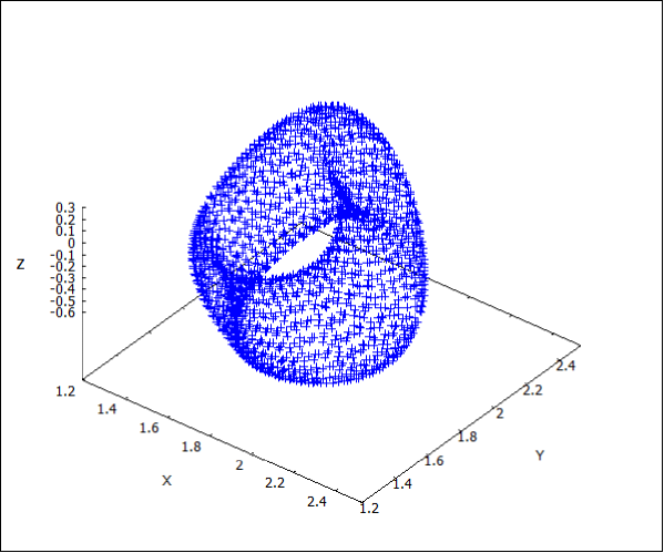
Figure 1: The 3D projection $(d_{n-1},d_{n},v_{n-1})$ of 2000 points on the orbit of the 4D map (3.29) with $f=-5$, $g=u=-1$ and $(d_{0},d_{1},v_{0},v_{1})=(5/4,2,-1/2,0)$.

4 Orthogonal polynomials and Hankel determinants

After removing the first term $a_{0}$, the continued fraction expansion (2.6) becomes

$$G=\cfrac{1}{a_{1}+\cfrac{1}{a_{2}+\cdots}}=\cfrac{1}{2u_{1}^{-1}(X+v_{1})+\cfrac{1}{2u_{2}^{-1}(X+v_{2})+\cdots}}.$$ (4.1)

A continued fraction of this form, where each partial quotient $a_{j}=a_{j}(X)$ is a linear function of $X$, is called a J-fraction [54]. If we multiply the main numerator and denominator by $u_{1}/2$ and apply (2.16), then this can be rewritten in its more classical form, that is

$$G=\cfrac{-2u_{0}^{-1}d_{1}}{X+v_{1}-\cfrac{d_{2}}{X+v_{2}-\cfrac{d_{3}}{X+v_{3}-\cdots}}},$$ (4.2)

from which we see that, up to an overall prefactor of $-2/u_{0}$, it is completely determined by the quantities $d_{n}$ and $v_{n}$. In this section we apply standard results on J-fractions and associated orthogonal polynomials, which lead directly to formulae for the quantities $d_{n}$ and $v_{n}$ in terms of ratios of Casorati determinants, and Hankel determinants in particular. This generalizes certain results obtained for $\mathrm{g}=1$ by Chang, Hu and Xin [11] to hyperelliptic curves of any genus $\mathrm{g}$.

In the neighbourhood of the point $\infty_{1}\in{\cal C}$, the function $G$ defined by (2.17) has the series expansion

$$G=\sum_{j\geq 1}s_{j-1}\,X^{-j}=s_{0}X^{-1}+s_{1}X^{-2}+s_{2}X^{-3}+\ldots,$$ (4.3)

which can be used to define a linear functional $<\cdot>:{\cal F}\to{\mathbb{C}}$ according to

$$<\Phi>=\frac{1}{2\pi\mathrm{i}}\oint_{\infty_{1}}\Phi\,G\,\mathrm{d}X,$$ (4.4)

for any function $\Phi\in{\cal F}$, where the integral is taken along any sufficiently small closed contour around $\infty_{1}$ (anticlockwise in the $X$ plane) that does not encircle the poles of $G$ at $(x_{0}^{(1)},y_{0}^{(1)}),\ldots,(x_{0}^{(\mathrm{g})},y_{0}^{(\mathrm{g})})$ and $\infty_{2}$. In other words, $G$ can be regarded as a moment generating function with moments

$$<X^{j}>=s_{j},\qquad j=0,1,2,\ldots,$$ (4.5)

although in general, for complex $s_{j}$, this may not be associated with some positive measure. The linear functional (4.4) also defines a scalar product between any pair of functions $\Phi$, $\Psi$, that is

$$<\,\Phi,\Psi\,>:=<\Phi\Psi>.$$ (4.6)

The convergents of (4.1) are the sequence of rational functions of $X$ given by

$$\frac{p_{0}}{q_{0}}=0,\quad\frac{p_{1}}{q_{1}}=\frac{1}{a_{1}},\quad\frac{p_{2}}{q_{2}}=\cfrac{1}{a_{1}+\cfrac{1}{a_{2}}},\quad\frac{p_{3}}{q_{3}}=\cfrac{1}{a_{1}+\cfrac{1}{a_{2}+\cfrac{1}{a_{3}}}},\quad\ldots,$$

where by convention one can take

$$p_{0}=0,\qquad q_{0}=1,$$ (4.7)

followed by

$$p_{1}=s_{0}=\frac{u_{1}}{2},\qquad q_{1}=X+v_{1}=X-\frac{s_{1}}{s_{0}},$$ (4.8)

and for all $j\geq 1$ $p_{j}(X)$ and $q_{j}(X)$ are polynomials of degrees $j-1$ and $j$ in $X$, respectively, where without loss of generality each $q_{j}$ is taken to be monic. The recursion for the convergents is essentially controlled by the same matrix (3.4) that appears in the classical theory of continued fraction expansions of numbers in ${\mathbb{R}}$. However, the entries of this matrix must be scaled in order to ensure that the $q_{j}$ are monic, making use of (2.16) to remove dependence on the prefactors $u_{j}$, to yield

$$\left(\begin{array}[]{cc}p_{n}&q_{n}\\ p_{n-1}&q_{n-1}\end{array}\right)=\left(\begin{array}[]{cc}X+v_{n}&-d_{n}\\ 1&0\end{array}\right)\left(\begin{array}[]{cc}p_{n-1}&q_{n-1}\\ p_{n-2}&q_{n-2}\end{array}\right),$$

which is equivalent to the three-term linear recurrence relation

$$q_{n}=(X+v_{n})\,q_{n-1}-d_{n}\,q_{n-2},\qquad n\geq 2,$$ (4.9)

for the sequence of polynomials $(q_{n})$, and the same for the sequence $(p_{n})$, with the initial conditions (4.7) and (4.8). From the linear recurrence it is clear that $p_{n}/s_{0}$ is monic for each $n$.

Due to the fact that each $a_{j}=\left\lfloor Y_{j}\right\rfloor$ is linear in $X$, it is straightforward to see by induction that the $n$th approximant $p_{n}/q_{n}$ satisfies

$$G-\frac{p_{n}}{q_{n}}=\cfrac{1}{a_{1}+\cfrac{1}{\cdots+\cfrac{1}{a_{n}+Y_{n+1}^{-1}}}}-\cfrac{1}{a_{1}+\cfrac{1}{\cdots+\cfrac{1}{a_{n}}}}=O\left(X^{-(2n+1)}\right),$$

and since $q_{n}$ has degree $n$ this implies that

$$p_{n}-Gq_{n}=O(X^{-(n+1)}),\qquad n=0,1,2,\ldots.$$ (4.10)

Given the requirement on the degrees of $p_{n}$ and $q_{n}$, by considering the terms at orders $X^{n-1},X^{n-2},\ldots,X^{-n}$, the equation (4.10) provides $n$ linear equations that determine the non-trivial coefficients of $q_{n}$ in terms of the coefficients $s_{j}$ in (4.3), and a further $n$ linear equations for the non-trivial coefficients of $p_{n}$ in terms of those of $q_{n}$ and the $s_{j}$. This leads to a standard formula for $q_{n}$, given explicitly in determinantal form as

$$q_{n}(X)=\frac{1}{\Delta_{n}}\,\left|\begin{array}[]{ccccc}s_{0}&s_{1}&\cdots&s_{n-1}&s_{n}\\ s_{1}&&\iddots&&\vdots\\ \vdots&\iddots&&&\vdots\\ s_{n-1}&\cdots&\cdots&\cdots&s_{2n-1}\\ 1&X&X^{2}&\cdots&X^{n}\end{array}\right|,$$ (4.11)

where $\Delta_{n}$ is the $n\times n$ Hankel determinant

$$\Delta_{n}=\left|\begin{array}[]{cccc}s_{0}&s_{1}&\cdots&s_{n-1}\\ s_{1}&&\iddots&\vdots\\ \vdots&\iddots&&\vdots\\ s_{n-1}&\cdots&\cdots&s_{2n-2}\end{array}\right|=\det(s_{i+j-2})_{i,j=1,\ldots,n}.$$ (4.12)

For what follows, we also need to introduce another determinant of Casorati type, obtained from the coefficients $s_{j}$ in (4.3) by shifting the last column of the Hankel matrix, namely

$$\Delta_{n}^{*}=\left|\begin{array}[]{ccccc}s_{0}&s_{1}&\cdots&s_{n-2}&s_{n}\\ s_{1}&&\iddots&\vdots&\vdots\\ \vdots&\iddots&&\vdots&\vdots\\ s_{n-2}&\cdots&\cdots&s_{2n-4}&s_{2n-2}\\ s_{n-1}&\cdots&\cdots&s_{2n-3}&s_{2n-1}\end{array}\right|.$$ (4.13)

We refer to the latter as a shifted Hankel determinant. By convention we set $\Delta_{0}=1$ and $\Delta_{0}^{*}=0$.

We can now state our main result about Hankel determinants and orthogonal polynomials.

Theorem 4.1.

The quantities $d_{n}$, $v_{n}$ that appear under iteration of the J-fraction expansion (4.2) of the function (2.17), which provide the two components (3.8) of the iterates of the birational map (3.11), are given in terms of Hankel and shifted Hankel determinants by

$$d_{n}=\frac{\Delta_{n}\Delta_{n-2}}{\Delta_{n-1}^{2}}\quad\mathrm{for}\,\,n\geq 2,\qquad v_{n}=\frac{\Delta_{n-1}^{*}}{\Delta_{n-1}}-\frac{\Delta_{n}^{*}}{\Delta_{n}}\quad\mathrm{for}\,\,n\geq 1,$$ (4.14)

where the entries are determined recursively by $s_{0}=u_{1}/2$ and, for $j\geq 1$,

$$s_{j}=-\sum_{i=2}^{\mathrm{g}+1}(k^{(\mathrm{g}+1-i)}+\pi_{1}^{(\mathrm{g}+1-i)})s_{j-i}+\frac{d_{1}}{s_{0}}\left(\sum_{i=0}^{j-2}s_{i}s_{j-2-i}+\sum_{\ell=3}^{\mathrm{g}+2}\sum_{i=0}^{j-\ell}\rho_{0}^{(\mathrm{g}+2-\ell)}s_{i}s_{j-\ell-i}\right)+\bar{s}_{j}$$ (4.15)

where

$$\bar{s}_{j}=\begin{cases}s_{0}\rho_{1}^{(\mathrm{g}-j)}&\mathrm{for}\,\,1\leq j\leq\mathrm{g},\\ 0&\mathrm{for}\,\,j\geq\mathrm{g}+1.\end{cases}$$

Furthermore, the polynomials $q_{j}$ that appear as the denominators of the convergents of the J-fraction are orthogonal with respect to the scalar product (4.6) associated with the series (4.3), that is

$$<\,q_{n},q_{m}\,>=h_{n}\,\delta_{nm},$$ (4.16)

where

$$h_{n}=\frac{\Delta_{n+1}}{\Delta_{n}}.$$

• The formulae in (4.14) are classical expressions for the coefficients appearing in the linear recurrence (4.9) for orthogonal polynomials. A direct proof is obtained by substituting (4.11) into the three-term recurrence and expanding in powers of $X$: the determinantal expression for $v_{n}$ appears immediately at order $X^{n}$, while at order $X^{n-1}$ one finds a formula for $d_{n}$ as a combination of four terms that can be condensed into a single ratio by applying various identities for determinants (which are collected in an appendix for completeness). To find the entries of the Hankel determinants recursively, note from (2.8) that $G=1/Y_{1}=(Y-P_{1})/Q_{0}$, hence $Y=Q_{0}G+P_{1}$ and

  $$Y^{2}=Q_{0}^{2}G^{2}+2Q_{0}P_{1}G+P_{1}^{2}=P_{1}^{2}+Q_{0}Q_{1},$$

  using (2.14), so that $G$ satisfies the quadratic equation

  $$P_{1}G+\frac{1}{2}Q_{0}G^{2}=\frac{1}{2}Q_{1}.$$ (4.17)

  Upon substituting the series (4.3) for $G$ and expanding the polynomial coefficients in (4.17) with the notation in (2.12) and (3.7), and making use of (2.16) to replace $u_{0}$, the recursion (4.15) results. Finally, the orthogonality of the sequence of polynomials $(q_{n})$ follows by a standard inductive argument using the three-term recurrence, also making use of the moments (4.5) with (4.11) to expand $\Delta_{n}^{2}<q_{n}^{2}>$ as a sum of $n+1$ products of determinants, only one of which is non-vanishing, which yields $<\,q_{n},q_{n}\,>=\Delta_{n+1}/\Delta_{n}=h_{n}$. ∎

Example 4.1.

The recursion for moments in the elliptic case: For $\mathrm{g}=1$ we use the same notation as in Example 3.1, and for the recursion (4.15) we have

$$s_{0}=u_{1}/2,\qquad s_{1}=-s_{0}v_{1}$$

and

$$s_{j}=-(2d_{1}+f)s_{j-2}+s_{0}^{-1}d_{1}\left(\sum_{i=0}^{j-2}s_{i}s_{j-2-i}-v_{0}\sum_{i=0}^{j-3}s_{i}s_{j-3-i}\right)$$ (4.18)

for all $j\geq 2$. To illustrate this with a particular numerical example, let us pick the curve

$$Y^{2}=(X^{2}-3)^{2}-4(X+2),$$ (4.19)

so that $f=-3$, $u=-1$, $v=-2$, and set $u_{0}=-2$, $d_{0}=1$, $v_{0}=-1$. This fixes the function

$$G=Y_{0}-a_{0}=\frac{1+\frac{1}{2}(X^{2}-3-Y)}{X+1}={X}^{-1}+{2}X^{-3}+X^{-4}+6X^{-5}+\cdots.$$ (4.20)

Then (3.16) produces the values $d_{1}=1$, $v_{1}=0$, which gives $s_{0}=u_{1}/2=-2d_{1}/u_{0}=1$ and $s_{1}=-s_{0}v_{1}=0$, and the coefficients of the series expansion (4.20) are obtained from the particular recurrence

$$s_{j}=s_{j-2}+\sum_{i=0}^{j-2}s_{i}s_{j-2-i}+\sum_{i=0}^{j-3}s_{i}s_{j-3-i},\quad j\geq 2.$$

This produces the sequence of moments

$$1,0,2,1,6,7,24,41,115,236,613,1380,\ldots,$$

and the corresponding sequence of Hankel determinants begins with

$$\Delta_{0}=\Delta_{1}=1,\quad\Delta_{2}=\left|\begin{array}[]{cc}1&0\\ 0&2\end{array}\right|=2,\quad\Delta_{3}=\left|\begin{array}[]{ccc}1&0&2\\ 0&2&1\\ 2&1&6\end{array}\right|=3,\quad\Delta_{4}=\left|\begin{array}[]{cccc}1&0&2&1\\ 0&2&1&6\\ 2&1&6&7\\ 1&6&7&24\end{array}\right|=7,\ldots,$$ (4.21)

which should remind the reader of (1.2).

Example 4.2.

The recursion for moments in genus 2: With the notation of Example 3.2, the recursion (4.15) for $\mathrm{g}=2$ has initial values

$$s_{0}=u_{1}/2,\qquad s_{1}=-s_{0}v_{1},\qquad s_{2}=s_{0}(w_{1}-d_{1}-f),$$

and subsequent coefficients in the series expansion (4.3) are determined for $j\geq 3$ by

$$s_{j}=-(2d_{1}+f)s_{j-2}-(2d_{1}e_{1}+g)s_{j-3}+s_{0}^{-1}d_{1}\left(\sum_{i=0}^{j-2}s_{i}s_{j-2-i}-v_{0}\sum_{i=0}^{j-3}s_{i}s_{j-3-i}+w_{0}\sum_{i=0}^{j-4}s_{i}s_{j-4-i}\right).$$ (4.22)

As a particular example, consider the curve

$$Y^{2}=(X^{3}-5X-1)^{2}-4(X^{2}+2X+3),$$

with $f=-5$, $g=u=-1$, $v=-2$, $w=3$, and choose $u_{0}=-4$, $d_{0}=5/4$, $e_{0}=3/5$, $v_{0}=-1/2$, $w_{0}=-3/2$, corresponding to the orbit of the map (3.29) plotted in Fig. 1, which gives

$$G=Y_{0}-a_{0}=\frac{X+\frac{1}{2}+\frac{1}{4}(X^{3}-5X-1-Y)}{X^{2}+\frac{1}{2}X-\frac{3}{2}}=X^{-1}+2X^{-3}+7X^{-5}+2X^{-6}+\cdots,$$

and the recursion for the coefficients (moments) in the above expansion is

$$s_{j}=s_{j-2}-s_{j-3}+2\sum_{i=0}^{j-2}s_{i}s_{j-2-i}+\sum_{i=0}^{j-3}s_{i}s_{j-3-i}-3\sum_{i=0}^{j-4}s_{i}s_{j-4-i},\quad j\geq 3$$

with initial values $s_{0}=1$, $s_{1}=0$, $s_{2}=2$. In this case, the sequence of moments $(s_{j})$ begins with

$$1,0,2,0,7,2,31,21,159,168,900,1246,5455,9040,34731,65328,\ldots,$$

yielding the corresponding sequence of Hankel determinants

$$(\Delta_{j}):\quad 1,1,2,6,31,319,5810,147719,8526736,\ldots,$$ (4.23)

as well as the sequence of shifted Hankel determinants

$$(\Delta_{j}^{*}):\quad 0,0,0,4,16,200,6987,161401,11022617,\ldots.$$

The map (3.11), or equivalently (3.12), corresponds to the recursion for the continued fraction expansion, and since this map is birational, it is also possible to reverse the direction of iteration and extend to all negative indices $n$ (again, this is always possible subject to the condition that $d_{n}$ does not vanish for some $n$). This immediately leads to a J-fraction expression for $Y_{0}$, that is

$$G^{\dagger}=Y_{0}=\cfrac{2u_{0}^{-1}d_{0}}{X+v_{-1}-\cfrac{d_{-1}}{X+v_{-2}-\cfrac{d_{-2}}{X+v_{-3}-\cdots}}},$$ (4.24)

which corresponds to a power series expansion around $\infty_{2}$,

$$G^{\dagger}=\sum_{j\geq 1}s_{j-1}^{\dagger}\,X^{-j}=s_{0}^{\dagger}X^{-1}+s_{1}^{\dagger}X^{-2}+s_{2}^{\dagger}X^{-3}+\ldots.$$ (4.25)

This means that the quantities $d_{n}$, $v_{n}$ can also be written in terms of ratios of determinants when $n$ is negative, but involving the Hankel determinant

$$\Delta_{n}^{\dagger}=\det(s_{i+j-2}^{\dagger})_{i,j=1,\ldots,n},$$

as well as the associated shifted Hankel determinant $\Delta_{n}^{\dagger*}$, which is just the analogue of (4.13) built from the coefficients in the series (4.25).

Theorem 4.2.

For negative indices $n$, the quantities $d_{n}$, $v_{n}$ that appear under iteration of the J-fraction expansion (4.24) of the function (2.3), which provide the two components (3.8) of the iterates of the birational map (3.11), are given in terms of Hankel and shifted Hankel determinants by

$$d_{1-n}=\frac{\Delta_{n}^{\dagger}\Delta_{n-2}^{\dagger}}{(\Delta_{n-1}^{\dagger})^{2}}\quad\mathrm{for}\,\,n\geq 2,\qquad v_{-n}=\frac{\Delta_{n-1}^{\dagger*}}{\Delta_{n-1}^{\dagger}}-\frac{\Delta_{n}^{\dagger*}}{\Delta_{n}^{\dagger}}\quad\mathrm{for}\,\,n\geq 1,$$ (4.26)

where the entries are determined recursively by $s_{0}^{\dagger}=-u_{-1}/2$ and, for $j\geq 1$,

$$s_{j}^{\dagger}=-\sum_{i=2}^{\mathrm{g}+1}(k^{(\mathrm{g}+1-i)}+\pi_{0}^{(\mathrm{g}+1-i)})s_{j-i}^{\dagger}+\frac{d_{0}}{s_{0}^{\dagger}}\left(\sum_{i=0}^{j-2}s_{i}^{\dagger}s_{j-2-i}^{\dagger}+\sum_{\ell=3}^{\mathrm{g}+2}\sum_{i=0}^{j-\ell}\rho_{0}^{(\mathrm{g}+2-\ell)}s_{i}^{\dagger}s_{j-\ell-i}^{\dagger}\right)+\bar{s}_{j}^{\dagger}$$ (4.27)

where

$$\bar{s}_{j}^{\dagger}=\begin{cases}s_{0}^{\dagger}\rho_{-1}^{(\mathrm{g}-j)}&\mathrm{for}\,\,1\leq j\leq\mathrm{g},\\ 0&\mathrm{for}\,\,j\geq\mathrm{g}+1.\end{cases}$$

• Since $G^{\dagger}=Y_{0}=(Y+P_{0})/Q_{0}$, the generating function for the moments $s_{j}^{\dagger}$ satisfies the quadratic equation $P_{0}G^{\dagger}-\frac{1}{2}Q_{0}(G^{\dagger})^{2}=-\frac{1}{2}Q_{-1}$, analogous to (4.17), and the recurrence (4.27) follows immediately after substituting in the series (4.25). Subject to suitable relabelling of indices, the derivation of the formulae is the same as in the proof of Theorem 4.1. ∎

Example 4.3.

Moments for negative $n$ in genus 2: Using the notation of Example 3.2 once again, the recursion (4.27) for $\mathrm{g}=2$ has initial values

$$s_{0}^{\dagger}=-u_{-1}/2,\qquad s_{1}^{\dagger}=-s_{0}^{\dagger}v_{-1},\qquad s_{2}^{\dagger}=s_{0}^{\dagger}(w_{-1}-d_{0}-f),$$

and subsequent coefficients in the series expansion (4.3) are determined for $j\geq 3$ by

$$s_{j}^{\dagger}=-(2d_{0}+f)s_{j-2}^{\dagger}-(2d_{0}e_{0}+g)s_{j-3}^{\dagger}+(s_{0}^{\dagger})^{-1}d_{0}\left(\sum_{i=0}^{j-2}s_{i}^{\dagger}s_{j-2-i}^{\dagger}-v_{0}\sum_{i=0}^{j-3}s_{i}^{\dagger}s_{j-3-i}^{\dagger}+w_{0}\sum_{i=0}^{j-4}s_{i}^{\dagger}s_{j-4-i}^{\dagger}\right).$$ (4.28)

In particular, taking the specific curve $Y^{2}=(X^{3}-5X-1)^{2}-4(X^{2}+2X+3)$ that was used for illustration in Example 4.2, with the same function $Y_{0}$, as before we have $f=-5$, $g=u=-1$, $u_{0}=-4$, $d_{0}=5/4$, $e_{0}=3/5$, $v_{0}=-1/2$, $w_{0}=-3/2$, and also $v_{-1}=-1/10$, $w_{-1}=-3/2$, which gives

$$G^{\dagger}=Y_{0}=-\frac{1}{4}\left(\frac{Y+X^{3}-\frac{5}{2}X+\frac{1}{2}}{X^{2}+\frac{1}{2}X-\frac{3}{2}}\right)=-\frac{5}{8}X^{-1}-\frac{1}{16}X^{-2}-\frac{45}{32}X^{-3}-\frac{25}{64}X^{-4}-\frac{757}{128}X^{-5}-\frac{801}{256}X^{-6}-\cdots,$$

with $X\to\infty$ and $Y\sim-X^{3}$, and the recursion for the coefficients (moments) in the above expansion is

$$s_{j}^{\dagger}=\frac{5}{2}s_{j-2}^{\dagger}-\frac{1}{2}s_{j-3}^{\dagger}-2\sum_{i=0}^{j-2}s_{i}^{\dagger}s_{j-2-i}^{\dagger}-\sum_{i=0}^{j-3}s_{i}^{\dagger}s_{j-3-i}^{\dagger}+3\sum_{i=0}^{j-4}s_{i}^{\dagger}s_{j-4-i}^{\dagger},\quad j\geq 3$$

with initial values $s_{0}^{\dagger}=-5/8$, $s_{1}^{\dagger}=-1/16$, $s_{2}^{\dagger}=45/32$. In this case, the sequence of moments $(s_{j}^{\dagger})$ begins

$$-\frac{5}{2^{3}},-\frac{1}{2^{4}},-\frac{45}{2^{5}},-\frac{25}{2^{6}},-\frac{757}{2^{7}},-\frac{801}{2^{8}},-\frac{14749}{2^{9}},-\frac{24361}{2^{10}},-\frac{316037}{2^{11}},-\frac{714865}{2^{12}},\ldots,$$

yielding the corresponding sequence of Hankel determinants

$$(\Delta_{j}^{\dagger}):\quad 1,-\frac{5}{2^{3}},\frac{7}{2^{3}},-\frac{303}{2^{7}},\frac{4091}{2^{9}},-\frac{63805}{2^{10}},\frac{3496637}{2^{12}},\ldots,$$ (4.29)

which has alternating signs.

Remark 4.1.

Given the two sets of formulae (4.14) and (4.26), it is natural to want to write $d_{n}$ and $v_{n}$ in the form

$$d_{n}=\frac{\tau_{n}\tau_{n-2}}{\tau_{n-1}^{2}},\qquad v_{n}=\frac{\tau_{n-1}^{*}}{\tau_{n-1}}-\frac{\tau_{n}^{*}}{\tau_{n}}$$ (4.30)

for all $n\in{\mathbb{Z}}$, for some set of quantities $\tau_{n},\tau_{n}^{*}$. However, in general one cannot just take $\tau_{n}=\Delta_{n}$ for non-negative $n$ and $\tau_{n}=\Delta_{-n-1}^{\dagger}$ for negative $n$ (and similarly for $\tau_{n}^{*}$) , because there will be a mismatch at the values of $d_{0},d_{1}$ and $v_{0}$ which are left unspecified by Theorems 4.1 and 4.2. Nevertheless, one can make use of the fact that the expressions for $d_{n}$ and $v_{n}$ in (4.30) are left invariant by the three-parameter group of gauge transformations

$$\tau_{n}\rightarrow ab^{n}\tau_{n},\qquad\tau_{n}^{*}\rightarrow ab^{n}(\tau_{n}^{*}+c\tau_{n}).$$ (4.31)

In particular, the choice

$$\tau_{n}=\begin{cases}\Delta_{n}&\mathrm{for}\,\,n\geq 0,\\ (-1)^{n}\left(\frac{2}{u_{0}}\right)^{2n+1}\Delta_{-n-1}^{\dagger}&\mathrm{for}\,\,n\leq-1\end{cases}$$

ensures that the values of $d_{0}$ and $d_{1}$ match up, and a similar choice can be made for $\tau_{n}^{*}$ to fix $v_{0}$. For instance, applying this choice to glue together the sequences (4.23) and (4.29) in a consistent fashion yields the doubly infinite sequence

$$(\tau_{n}):\quad\ldots,562196701,6993274,127610,4091,303,28,5,2,1,1,2,6,31,319,5810,147719,\ldots.$$ (4.32)

5 The Somos connection

In this section, we explain how Somos sequences naturally arise from the continued fraction expansion, as quadratic relations for the Hankel determinants $\Delta_{n}$. This is most straightforward to describe in the genus one case, as it follows from the fact that, for a fixed value of the first integral $H=-uv$ given by (3.17), each orbit of (3.16) coincides with an orbit of a symmetric QRT map, and, as was already noted in [47] in an example related to the hard hexagon model, the bilinear form of the latter is precisely (1.1). (For a detailed discussion of normal forms of QRT maps restricted to fixed invariant curves, see [29, 30].)

Proposition 5.1.

For a fixed value of the first integral $H=-uv$, on each orbit of the map (3.16) the quantity $d_{n}$ satisfies the second order recurrence

$$d_{n+1}d_{n-1}=\frac{{\alpha}\,d_{n}+{\beta}}{d_{n}^{2}},$$ (5.1)

with coefficients ${\alpha}=u^{2}$, ${\beta}=u^{2}(v^{2}+f)$.

• Putting $X=v_{n}$ into (3.15) and then applying the first equation in (3.14) yields

  $$u(v_{n}-v)=d_{n}(d_{n}+v_{n}^{2}+f)=-d_{n}d_{n+1}.$$

  Then putting $X=v$ into (3.15) and using the above result gives

  $$\begin{array}[]{rcl}0&=&d_{n}\Big{(}v^{2}+f-(v-v_{n-1})(v-v_{n})+d_{n}\Big{)}\\ &=&d_{n}\Big{(}v^{2}+f-u^{-2}d_{n+1}d_{n}^{2}d_{n-1}+d_{n}\Big{)},\end{array}$$

  so that (5.1), which is an example of a symmetric QRT map [47], follows immediately. ∎

The connection with Somos-4 is almost immediate, since if $d_{n}=\tau_{n}\tau_{n-2}/(\tau_{n-1})^{2}$, then $\tau_{n}$ satisfies (1.1) whenever $d_{n}$ satisfies (5.1). So in particular, by Theorem 4.1, the Hankel determinants for $\mathrm{g}=1$ satisfy a Somos-4 relation, and since the latter is invariant under the first of the gauge transformations (4.31), any Somos-4 sequence can be expressed in terms of Hankel determinants. More precisely, starting from any Somos-4 sequence, one can always make a gauge transformation to a sequence with $\tau_{0}=1$, and then use the coefficients ${\alpha},{\beta}$ and the other initial conditions $\tau_{1},\tau_{2},\tau_{3}$ to specify the values of $s_{0}=\Delta_{1}=\tau_{1}$ and $v_{0},v_{1},d_{1},f$, so that the values of $s_{1}$ and the coefficients in (4.18) are fixed. (In fact, since the gauge transformation involves two parameters $a,b$, there is also the freedom to fix $\tau_{1}=1$, which corresponds to taking $s_{0}=1$.) Thus we arrive at the following result.

Theorem 5.2.

In the case $\mathrm{g}=1$, the Hankel determinants (4.12) with moments defined recursively by (4.18) satisfy the Somos-4 recurrence

$$\Delta_{n+4}\Delta_{n}={\alpha}\,\Delta_{n+3}\Delta_{n+1}+{\beta}\,\Delta_{n+2}^{2},$$ (5.2)

with

$${\alpha}=u^{2},\qquad{\beta}=u^{2}(v^{2}+f).$$ (5.3)

Moreover, every solution of the Somos-4 recurrence (1.1) can be written in the form

$$\tau_{n}=\begin{cases}\hat{a}\hat{b}^{n}\Delta_{n}&\mathrm{for}\,\,n\geq 0,\\ a^{\dagger}(b^{\dagger})^{n}\Delta_{-n-1}^{\dagger}&\mathrm{for}\,\,n\leq-1,\end{cases}$$

where $\Delta_{n}^{\dagger}$ is constructed from moments that satisfy (4.27) with $\mathrm{g}=1$, for suitable constants $\hat{a},\hat{b},a^{\dagger},b^{\dagger}$.

There is an apparent mismatch between the Hankel determinants in (1.7), which were shown by Xin to yield the terms of the Somos-4 sequence (1.2), and those in (4.21) above. We now explain the relation between these two sets of Hankel determinant formulae, and see how the results of [11] are a consequence of the continued fraction expansion for $\mathrm{g}=1$.

Theorem 5.3.

For $n\geq 2$, the quantity $d_{n}$ that satisfies (3.16) is given by

$$d_{n}=\frac{D_{n}D_{n-2}}{D_{n-1}^{2}},$$ (5.4)

in terms of the Hankel determinant (1.4) defined in terms of moments $\tilde{s}_{j}$ that satisfy the recursion (1.8) for $j\geq 2$, with

$$\tilde{s}_{0}=u_{1}/2,\quad\tilde{s}_{1}=-\tilde{s}_{0}(v_{0}+v_{1}),\quad\tilde{{\alpha}}=-2v_{0},\quad\tilde{{\beta}}=d_{0}-d_{1},\quad\tilde{{\gamma}}=\frac{d_{1}}{\tilde{s}_{0}}.$$

Moreover, the sequence $(D_{n})_{n\geq 0}$ is identical to the sequence of Hankel determinants $(\Delta_{n})_{n\geq 0}$ with moments satisfying (4.18), hence satisfies the Somos-4 recurrence (5.2) with coefficients as in (5.3).

• By replacing $X$ with the shifted variable $\tilde{X}=X-v_{0}$, and letting $\tilde{G}(\tilde{X})=G(X)$, we obtain the J-fraction

  $$\tilde{G}=\cfrac{-2\tilde{u}_{0}^{-1}\tilde{d}_{1}}{\tilde{X}+\tilde{v}_{1}-\cfrac{\tilde{d}_{2}}{\tilde{X}+\tilde{v}_{2}-\cfrac{\tilde{d}_{3}}{\tilde{X}+\tilde{v}_{3}-\cdots}}}=\sum_{j\geq 1}\tilde{s}_{j-1}\tilde{X}^{-j},$$ (5.5)

  where, from (4.17) in the case $\mathrm{g}=1$, the generating function $\tilde{G}$ satisfies

  $$\Big{(}\tilde{X}^{2}+2v_{0}\tilde{X}+(v_{0}^{2}+2d_{1}+f)\Big{)}\tilde{G}+\frac{u_{0}}{2}\tilde{X}\tilde{G}^{2}=\frac{u_{1}}{2}(\tilde{X}+v_{0}-v_{1}).$$ (5.6)

  In the first line of the continued fraction (5.5), we are at liberty to choose $\tilde{u}_{0}=u_{0}$, which implies that $\tilde{d}_{1}=d_{1}$, and then in each subsequent line we have $\tilde{v}_{n}=v_{n}+v_{0}$ for $n\geq 1$, and also $\tilde{d}_{n}=d_{n}$ for $n\geq 2$. Hence, by the same argument as in the proof of Theorem 4.1, the formula (5.4) holds for $n\geq 2$. The moments $\tilde{s}_{j}$ are obtained from the series expansion of $\tilde{G}$ in powers of $\tilde{X}$, with the leading order term (order $\tilde{X}$) in (5.6) giving $\tilde{s}_{0}=s_{0}=u_{1}/2$, and the next to leading order term (order $\tilde{X}^{0}$) giving $\tilde{s}_{1}+2v_{0}\tilde{s}_{0}=\frac{u_{1}}{2}(v_{0}-v_{1})$, while at order $\tilde{X}^{-j+1}$ for $j\geq 2$, upon noting that $\tilde{{\beta}}=-v_{0}^{2}-2d_{1}-f=d_{0}-d_{1}$ from (3.16), we find the recursion relation (1.8) with the stated values of $\tilde{{\alpha}},\tilde{{\beta}},\tilde{{\gamma}}$. By convention we have $D_{0}=\Delta_{0}=1$, and also $D_{1}=\tilde{s}_{0}=s_{0}=\Delta_{1}$, and then it follows by induction from (5.4) that $D_{n}=\Delta_{n}$ for all $n\geq 0$. ∎

Remark 5.1.

In order to see how Xin’s result [56] follows from the above, it is sufficient to note that the quartic curve (4.19) is isomorphic to (1.5), via the birational equivalence $Y=x^{-2}(1-2\eta)$, $X=\tilde{X}-1=x^{-1}-1$, so that the expansion (1.6) in powers of $x$ is equivalent to an expansion in powers of $\tilde{X}^{-1}$. Also, by setting $\eta=(1-y)/2$, the Weierstrass cubic $y^{2}=4x^{3}-4x+1$ derived from analytic formulae in [23] is seen to be isomorphic to the curve (1.5); over ${\mathbb{Q}}$, this is known as 37a1, the elliptic curve of minimal conductor with positive rank. (See www.lmfdb.org/EllipticCurve/Q/37/a/1 in the online database of L-functions, modular forms, and related objects.)

The analogue of Theorem 5.2 in genus two is more difficult to state explicitly, due to the size of the expressions for the coefficients, and at present we are only able to prove it with the use of computer algebra.

Theorem 5.4.

In the case $\mathrm{g}=2$, the Hankel determinants (4.12) with moments defined recursively by (4.22) satisfy a Somos-8 recurrence of general type, that is

$${\alpha}_{1}\,\Delta_{n+8}\Delta_{n}+{\alpha}_{2}\,\Delta_{n+7}\Delta_{n+1}+{\alpha}_{3}\,\Delta_{n+6}\Delta_{n+2}+{\alpha}_{4}\,\Delta_{n+5}\Delta_{n+3}+{\alpha}_{5}\,\Delta_{n+4}^{2}=0,$$ (5.7)

where the coefficients ${\alpha}_{1},\ldots,{\alpha}_{5}$ are certain first integrals of the map (3.29).

• The recurrence (5.7) is equivalent to a relation for the iterates $d_{n}$, that is

  $${\alpha}_{1}d_{n+8}d_{n+7}^{2}d_{n+6}^{3}d_{n+5}^{4}d_{n+4}^{3}d_{n+3}^{2}d_{n+2}+{\alpha}_{2}d_{n+7}d_{n+6}^{2}d_{n+5}^{3}d_{n+4}^{2}d_{n+3}+{\alpha}_{3}d_{n+6}d_{n+5}^{2}d_{n+4}+{\alpha}_{4}d_{n+5}+{\alpha}_{5}=0,$$

  along an orbit of the 4D map (3.29). Equivalently, writing a solution of this map in the form (4.30), it means that $\tau_{n}$ should satisfy the Somos-8 recurrence (5.7) with some coefficients ${\alpha}_{j}$ that are constant on each orbit. This requires the vanishing of a $5\times 5$ determinant, namely

  $$\left|\begin{array}[]{ccccc}\tau_{n+4}\tau_{n-4}&\tau_{n+3}\tau_{n-3}&\tau_{n+2}\tau_{n-2}&\tau_{n+1}\tau_{n-1}&\tau_{n}^{2}\\ \tau_{n+5}\tau_{n-3}&\cdots&\cdots&\cdots&\tau_{n+1}^{2}\\ \vdots&&&&\vdots\\ \tau_{n+8}\tau_{n}&\cdots&\cdots&\cdots&\tau_{n+4}^{2}\end{array}\right|=0$$ (5.8)

  for all $n$, and also that the ratios of certain $4\times 4$ minors should be independent of $n$. In particular, denoting by $\hat{D}_{j,n}$ the minor formed from the first four rows in (5.8) with the $j$th column removed, so that

  $$\hat{D}_{1,n}=\left|\begin{array}[]{cccc}\tau_{n+3}\tau_{n-3}&\tau_{n+2}\tau_{n-2}&\tau_{n+1}\tau_{n-1}&\tau_{n}^{2}\\ \tau_{n+4}\tau_{n-2}&\cdots&\cdots&\tau_{n+1}^{2}\\ \tau_{n+5}\tau_{n-1}&\cdots&\cdots&\tau_{n+2}^{2}\\ \tau_{n+6}\tau_{n}&\cdots&\cdots&\tau_{n+3}^{2}\end{array}\right|,$$

  and so on, the existence of the relation (5.7) for $\tau_{n}$ is equivalent to the requirement that the ratios

  $$\frac{{\alpha}_{j}}{{\alpha}_{1}}=\hat{D}_{j,n}/\hat{D}_{1,n},\qquad j=2,3,4,5$$

  are independent of $n$ (noting the possibility of a vanishing denominator, in the case that ${\alpha}_{1}=0$). So in order to verify the statement, it is sufficient to check that

  $$\hat{D}_{j,n}\hat{D}_{1,n+1}-\hat{D}_{j,n+1}\hat{D}_{1,n}=0,$$ (5.9)

  holds for each $j=2,3,4,5$, and for all $n$. In fact, for each $j$, it is enough to check that this holds for a single shift $n\to n+1$ with arbitrary initial data in the map (3.29), which guarantees that each of the ratios ${\alpha}_{j}/{\alpha}_{1}$ is a first integral, and then it automatically holds for all $n$. Even with the help of computer algebra, this is not a completely straightforward task, and in order to do it as efficiently as possible it is convenient to make a gauge transformation (4.31) to fix $s_{0}=1$, and then note that there is a one-to-one correspondence between two sets of seven parameters: the four initial values $d_{0},d_{1},v_{0},v_{1}$ and three parameters $f,g,u$ needed to iterate the map (3.29), and the two initial values $s_{1},s_{2}$ and five coefficients $\tilde{{\alpha}},\tilde{{\beta}},\tilde{{\gamma}},\tilde{\delta},\tilde{\epsilon}$ that specify the genus two recursion (4.22) in the form

  $$s_{j}=\tilde{{\alpha}}s_{j-2}+\tilde{{\beta}}s_{j-3}+\tilde{{\gamma}}\sum_{i=0}^{j-2}s_{i}s_{j-2-i}+\tilde{\delta}\sum_{i=0}^{j-3}s_{i}s_{j-3-i}+\tilde{\epsilon}\sum_{i=0}^{j-4}s_{i}s_{j-4-i}.$$

  Now, using the above recursion, one can calculate the sequence $(s_{j})_{j\geq 0}$, and then compute the Hankel determinants $\tau_{n}=\Delta_{n}$ for $n=0,1,2,\ldots$, which are polynomials in ${\mathbb{Z}}[s_{1},s_{2},\tilde{{\alpha}},\tilde{{\beta}},\tilde{{\gamma}},\tilde{\delta},\tilde{\epsilon}]$, but this rapidly becomes very computationally intensive as $n$ increases. More efficient is to rewrite the map (3.29) as an equivalent pair of coupled recurrence relations of degree 6 for $\tau_{n},\tau_{n}^{*}$, which are of overall order 7. To iterate the latter, one needs 7 initial values (four adjacent $\tau_{n}$ and three adjacent $\tau_{n}^{*}$), and it is convenient to take $\tau_{0}=\Delta_{1}=1$, $\tau_{1}=\Delta_{0}=s_{0}=1$ but also $\tau_{-1}=d_{1}=\tilde{{\gamma}}$ and $\tau_{-2}=\tilde{{\gamma}}^{2}d_{0}=\tilde{{\alpha}}\tilde{{\gamma}}+\tilde{{\gamma}}^{3}-\tilde{\delta}^{2}+\tilde{{\gamma}}\tilde{\epsilon}$, together with $\tau_{0}^{*}=\Delta_{0}^{*}=0$, $\tau_{1}^{*}=\Delta_{1}^{*}=s_{1}$, as well as $\tau_{-1}^{*}=d_{1}v_{0}=-\tilde{\delta}$, noting that $f=-\tilde{{\alpha}}-2\tilde{{\gamma}}$, $g=-\tilde{{\beta}}-2\tilde{{\gamma}}s_{1}-2\tilde{\delta}$, $u=-\tilde{{\gamma}}s_{2}-\tilde{\delta}s_{1}-\tilde{\epsilon}$. The verification of (5.9) requires 13 adjacent values of $\tau_{n}$, but due to the size of the expressions involved it is best to compute only up to $\tau_{6}$ using five forward steps of the coupled recurrence for $\tau_{n},\tau_{n}^{*}$, and then apply this recurrence in reverse, making four backward steps to go back as far as $\tau_{-6}$, so that the adjacent values $\tau_{-6},\tau_{-5},\ldots,\tau_{5},\tau_{6}$ are obtained as explicit polynomials in ${\mathbb{Z}}[s_{1},s_{2},\tilde{{\alpha}},\tilde{{\beta}},\tilde{{\gamma}},\tilde{\delta},\tilde{\epsilon}]$. This means that the minors $\hat{D}_{j,-2}$ and $\hat{D}_{j,-1}$ can be computed explicitly, which allows (5.9) to be checked directly when $n=-2$. The formulae for the first integrals ${\alpha}_{j}/{\alpha}_{1}$, $j=2,3,4,5$ as rational functions of $s_{1},s_{2},\tilde{{\alpha}},\tilde{{\beta}},\tilde{{\gamma}},\tilde{\delta},\tilde{\epsilon}$ are so large that they are difficult to display even on a computer screen, but if ${\alpha}_{1}$ is regarded as the first integral that is the lowest common denominator of these four quantities, then we arrive at the Somos-8 relation (5.7). ∎

Example 5.1.

The doubly infinite sequence (4.32), which extends (4.23), satisfies the Somos-8 relation

$$7\tau_{n+8}\tau_{n}+137\tau_{n+7}\tau_{n+1}+2504\tau_{n+6}\tau_{n+2}-43424\tau_{n+5}\tau_{n+3}-26959\tau_{n+4}^{2}=0.$$

Remark 5.2.

As already noted, there is the possibility of a vanishing denominator ${\alpha}_{1}=0$ in the ratios ${\alpha}_{j}/{\alpha}_{1}$, $j=2,3,4,5$. Given that the map (3.29) only has two independent first integrals, which can be specified by $H_{1}=-uv,H_{2}=uw$ as in (3.26) and (3.27), it follows that these four ratios are rational functions of $f,g,u,H_{1},H_{2}$, with coefficients in ${\mathbb{Q}}$, so that ${\alpha}_{1}$ can be fixed as the polynomial in ${\mathbb{Z}}[f,g,u,H_{1},H_{2}]$ that is the lowest common denominator of these four rational functions. Thus it can happen that ${\alpha}_{1}=0$ for certain combinations of $f,g,u,H_{1},H_{2}$, in which case $\Delta_{n}$ (or $\tau_{n}$) satisfies a Somos-6 relation, rather than a Somos-8. Numerical experiments suggest that $u|{\alpha}_{1}(f,g,u,H_{1},H_{2})$, consistent with a result of van der Poorten, who showed that there is a Somos-6 relation in the special case $u=0$ [45, 46].

Before concluding this section, we state a conjecture which is the genus two analogue of Theorem 1.1.

Conjecture 5.5.

When $\mathrm{g}=2$, the Hankel determinants (4.12) with moments defined by (4.22) are given by

$$\Delta_{n}=\hat{a}\hat{b}^{n}\,\frac{{\sigma}({\bf z}_{0}+n{\bf z})}{{\sigma}({\bf z})^{n^{2}}},$$ (5.10)

in terms of the genus two Kleinian sigma function ${\sigma}({\bf z})={\sigma}({\bf z};\tilde{c}_{0},\tilde{c}_{1},\tilde{c}_{2},\tilde{c}_{3})$ associated with a quintic curve $\tilde{{\cal C}}$ that is isomorphic to the sextic ${\cal C}$ in (3.19), given by $\tilde{{\cal C}}:\,y^{2}=4x^{5}+\sum_{j=0}^{3}\tilde{c}_{j}x^{j}$ with period lattice $\Lambda$, for ${\bf z}_{0}$, ${\bf z}\in{\mathbb{C}}^{2}\bmod\Lambda$ with ${\bf z}=2\int_{\infty}^{\tilde{P}_{2}}(\frac{\mathrm{d}x}{y},\frac{x\mathrm{d}x}{y})^{T}$, where $\infty$ is the unique point at infinity on $\tilde{{\cal C}}$, $\tilde{P}_{2}\in\tilde{{\cal C}}$ is the point corresponding to $\infty_{2}\in{\cal C}$, and $\hat{a},\hat{b}$ are certain non-zero constants.

A proof of the above result would follow from an analytic solution for the iterates of the map (3.29), which we propose to consider elsewhere. However, to see why this result is plausible we note that since the class of the divisor $\tilde{P}_{2}-\tilde{P}_{1}\sim_{\mathrm{lin}}2(\tilde{P}_{2}-\infty)$ in the Jacobian of $\tilde{{\cal C}}$ corresponds to that of the divisor $\infty_{2}-\infty_{1}$ on ${\cal C}$, each shift $n\to n+1$ increases the argument of the numerator in (5.10) by ${\bf z}$, which is consistent with (2.18). Furthermore, if the formula (5.10) is correct then, by essentially the same analytical calculations as those in [7, 26], it follows immediately that $\Delta_{n}$ satisfies the Somos-8 relation (5.7), or a Somos-6 relation when a certain constraint on ${\bf z}$ holds.

In the higher genus case, we further conjecture that there should be an analytical formula analogous to (5.10). Equivalently, there should be an expression in terms of the Riemann theta function associated with the Jacobian of the curve (2.1), of the form $\Delta_{n}=\hat{a}\hat{b}^{n}\hat{c}^{n^{2}}\Theta({\bf v}_{0}+n{\bf v})$ for some $\hat{a},\hat{b},\hat{c}\in{\mathbb{C}}^{*}$ and ${\bf v}_{0},{\bf v}\in{\mathbb{C}}^{\mathrm{g}}$. If this expression holds, then by counting the dimension of the vector space of quasiperiodic functions of weight 2 with respect to the period lattice (see [39]), it follows that $\Delta_{n}$ satisfies a Somos-$k$ relation for some $k\leq 2^{\mathrm{g}+1}$. We have verified this in numerical examples for $\mathrm{g}=3,4$.

6 Poisson structure and integrability

In this section we slightly change our notation, and consider a modified family of Lax matrices, given by

$${\cal L}({\zeta})=\left(\begin{array}[]{cc}\mathrm{P}({\zeta})&\mathrm{R}({\zeta})\\ \mathrm{Q}({\zeta})&-\mathrm{P}({\zeta})\end{array}\right),$$ (6.1)

where $\mathrm{P}$ and $\mathrm{R}$ are monic polynomials of degrees $\mathrm{g}+1$ and $\mathrm{g}$ in ${\zeta}$, respectively, and $\mathrm{Q}$ is a polynomial of degree $\mathrm{g}$ with non-constant leading coefficient, which we write as

$$\mathrm{Q}=-4d_{0}{\zeta}^{\mathrm{g}}+O({\zeta}^{\mathrm{g}-1}).$$

The set of all such matrices forms an affine space of dimension $3\mathrm{g}+2$, with coordinates given by the non-trivial coefficients of $\mathrm{P}$, $\mathrm{Q}$ and $\mathrm{R}$. We will endow this space with a particular Poisson structure of rank $2\mathrm{g}$, and show how this leads to the construction of an associated set of Hamiltonian vector fields that are completely integrable in the Liouville sense. Then we will present a compatible discrete integrable system on the same phase space, and show that this is equivalent to the iteration of the recursion for the continued fraction expansion of the hyperelliptic function considered previously.

The Poisson brackets between the entries of $\cal L$ are specified by

$$\{\,\mathrm{P}({\zeta}),\mathrm{P}(\eta)\,\}=0\,=\,\{\,\mathrm{R}({\zeta}),\mathrm{R}(\eta)\,\},$$ (6.2)

$$\{\,\mathrm{P}({\zeta}),\mathrm{Q}(\eta)\,\}=2\left(\frac{\mathrm{Q}({\zeta})-\mathrm{Q}(\eta)}{{\zeta}-\eta}\right),\quad\{\,\mathrm{P}({\zeta}),\mathrm{R}(\eta)\,\}=-2\left(\frac{\mathrm{R}({\zeta})-\mathrm{R}(\eta)}{{\zeta}-\eta}\right),$$ (6.3)

$$\{\,\mathrm{Q}({\zeta}),\mathrm{Q}(\eta)\,\}=-4\Big{(}\mathrm{Q}({\zeta})-\mathrm{Q}(\eta)\Big{)},\quad\{\,\mathrm{Q}({\zeta}),\mathrm{R}(\eta)\,\}=4\left(\frac{\mathrm{P}({\zeta})-\mathrm{P}(\eta)}{{\zeta}-\eta}\right)-4\mathrm{R}(\eta).$$ (6.4)

In terms of the coefficients appearing in $\cal L$, this is a linear bracket, since the right-hand sides are linear in $\mathrm{P}$, $\mathrm{Q}$, $\mathrm{R}$. In order for this to define a Poisson bracket, it must satisfy the Jacobi identity, and although this can be verified directly this requires many tedious calculations; we set this question aside for now, and a simpler argument will be presented in due course.

To begin with, we consider the function

$$F({\zeta})=-\det{\cal L}({\zeta})=\mathrm{P}({\zeta})^{2}+\mathrm{Q}({\zeta})\mathrm{R}({\zeta}).$$ (6.5)

Using the above bracket relations, we find that

$$\{\,\mathrm{P}({\zeta}),F(\eta)\,\}=2\left(\frac{\mathrm{Q}({\zeta})\mathrm{R}(\eta)-\mathrm{Q}(\eta)\mathrm{R}({\zeta})}{{\zeta}-\eta}\right),$$ (6.6)

$$\{\,\mathrm{Q}({\zeta}),F(\eta)\,\}=4\left(\frac{\mathrm{P}({\zeta})\mathrm{Q}(\eta)-\mathrm{P}(\eta)\mathrm{Q}({\zeta})}{{\zeta}-\eta}\right)-4\mathrm{Q}({\zeta})\mathrm{R}(\eta),$$ (6.7)

$$\{\,\mathrm{R}({\zeta}),F(\eta)\,\}=4\left(\frac{\mathrm{P}(\eta)\mathrm{R}(\zeta)-\mathrm{P}(\zeta)\mathrm{R}(\eta)}{{\zeta}-\eta}\right)+4\mathrm{R}({\zeta})\mathrm{R}(\eta).$$ (6.8)

It is straightforward to check that the right-hand sides of the above expressions are polynomials in $\eta$ of degrees $\mathrm{g}-2$, $\mathrm{g}-1$, $\mathrm{g}-1$ respectively. Thus, if we expand

$$F(\eta)=\eta^{2\mathrm{g}+2}+\sum_{j=0}^{2\mathrm{g}+1}c_{j}{\zeta}^{j},$$ (6.9)

then these expressions imply that

$$\{\,\cdot\,,c_{j}\,\}=0\quad\mathrm{for}\quad j=\mathrm{g},\mathrm{g}+1,\ldots,2\mathrm{g}+1,$$

or in other words the leading $\mathrm{g}+2$ non-trivial coefficients of $F$ are Casimirs.

In fact $c_{\mathrm{g}},\ldots,c_{2\mathrm{g}+1}$ provide the full set of Casimirs, and the symplectic leaves have dimension $2\mathrm{g}$. To see this, factorize $\mathrm{R}$ as

$$\mathrm{R}({\zeta})=\prod_{i=1}^{\mathrm{g}}({\zeta}-x_{i}),$$ (6.10)

and set

$$y_{i}=\mathrm{P}(x_{i}),\qquad i=1,\ldots,\mathrm{g}.$$ (6.11)

Then

$$\mathrm{P}({\zeta})={\zeta}^{\mathrm{g}+1}+\frac{1}{2}c_{2\mathrm{g}+1}{\zeta}^{\mathrm{g}}+\sum_{j=0}^{\mathrm{g}-1}\pi_{j}{\zeta}^{j},$$

where, from (6.11), the $\mathrm{g}$ coefficients $\pi_{j}$ can be found explicitly as functions of the $x_{i}$, the $y_{i}$ and the Casimir $c_{2\mathrm{g}+1}$ by solving a linear system. The two relations in (6.2) then imply that

$$\{\,x_{i},x_{j}\,\}=0=\{\,y_{i},y_{j}\,\}$$

for all $i,j$, while from the second bracket in (6.3) it follows that

$$\{\,y_{i},x_{j}\,\}=2\delta_{ij},$$

so that (up to scaling) the pairs $(x_{i},y_{i})_{i=1,\ldots,\mathrm{g}}$ provide a set of canonical coordinates on a symplectic manifold of dimension $2\mathrm{g}$, and by (6.5), for fixed values of the coefficients $c_{j}$ in (6.9), each pair $({\zeta},\mu)=(x_{i},y_{i})$ is a point on the spectral curve

$$\mu^{2}=F(\zeta).$$ (6.12)

Then by using (6.10), (6.11) and the leading terms in (6.5) up to and including order ${\zeta}^{g}$, all of the coefficients in $\cal L$ can be expressed as functions of the $x_{i}$, $y_{i}$ and the Casimirs, so the whole Poisson algebra is expressed in terms of these coordinates.

The latter argument begs the question of whether the Poisson brackets for the entries of $\cal L$ satisfy the Jacobi identity in the first place, but this is easily seen by reversing the direction of the preceding argument. Indeed, starting with the canonical bracket between the $x_{i}$ and $y_{j}$, one extends it with the Casimirs $c_{\mathrm{g}},\ldots,c_{2\mathrm{g}+1}$ to obtain a Poisson algebra of dimension $3\mathrm{g}+2$, where the entries of $\cal L$ are defined in terms of these canonical coordinates as above, and by construction they satisfy the linear bracket relations given before. Hence the Jacobi identity is trivially satisfied.

We now consider a family of vector fields on the space of Lax matrices, defined by the flow

$$\frac{\mathrm{d}}{\mathrm{d}t}{\cal L}({\zeta})=\{\,{\cal L}({\zeta}),F(\eta)\,\}.$$ (6.13)

From the bracket relations (6.6), (6.7), (6.8), it can be verified directly that this can be written in the form of a Lax equation, that is

$$\frac{\mathrm{d}}{\mathrm{d}t}{\cal L}({\zeta})=[{\cal P}({\zeta},\eta),{\cal L}({\zeta})],$$

with the matrix

$${\cal P}({\zeta},\eta)=\frac{2}{{\zeta}-\eta}\left(\begin{array}[]{cc}\mathrm{P}(\eta)+({{\zeta}-\eta})\mathrm{R}(\eta)&\mathrm{R}(\eta)\\ \mathrm{Q}(\eta)&-\mathrm{P}(\eta)-({{\zeta}-\eta})\mathrm{R}(\eta)\end{array}\right).$$ (6.14)

Moreover, all the flows in this family commute with one another, because the same bracket relations imply that

$$\{\,F({\zeta}),F(\eta)\,\}=2\mathrm{P}({\zeta})\{\,\mathrm{P}({\zeta}),F(\eta)\,\}+\mathrm{R}({\zeta})\{\,\mathrm{Q}({\zeta}),F(\eta)\,\}+\mathrm{Q}({\zeta})\{\,\mathrm{R}({\zeta}),F(\eta)\,\}=0.$$ (6.15)

Thus it follows that all of the coefficients $c_{j}$ in (6.9) are in involution, and in order to get non-trivial flows we can take the non-Casimir functions (Hamiltonians)

$$H_{j}=c_{j}=\mathrm{res}\,\frac{F(\eta)}{\eta^{j+1}}\Big{|}_{\eta=0},\qquad j=0,1,\ldots,\mathrm{g}-1.$$ (6.16)

Then since $\{\,H_{j},H_{k}\,\}=0$ for all $j,k$, this gives $\mathrm{g}$ commuting flows which can be written in Lax form as

$$\frac{\mathrm{d}}{\mathrm{d}t_{j}}{\cal L}({\zeta})=\{\,{\cal L}({\zeta}),H_{j}\,\}=[{\cal P}^{(j)}({\zeta}),{\cal L}({\zeta})],$$

where, for $j=0,\ldots,\mathrm{g}-1$, the matrix ${\cal P}^{(j)}$ is defined from (6.14) by

$${\cal P}^{(j)}({\zeta})=\mathrm{res}\,\frac{{\cal P}({\zeta},\eta)}{\eta^{j+1}}\Big{|}_{\eta=0}.$$

Hence we have integrability in the sense of Liouville [1].

Theorem 6.1.

The Hamiltonians (6.16) define a completely integrable system on the space of Lax matrices (6.1).

In fact, there is more that one can say: for fixed values of $c_{j}$ in (6.9), the set of triples of polynomials $\mathrm{P}({\zeta}),\mathrm{Q}({\zeta}),\mathrm{R}({\zeta})$ of the specified form that satisfy (6.5) for a fixed set of coefficients $c_{j}$ in (6.9) is an affine algebraic variety of dimension $\mathrm{g}$, that is canonically isomorphic to the affine Jacobian of the corresponding hyperelliptic spectral curve (6.12), by associating each such triple with the degree $\mathrm{g}$ divisor

$$D=(x_{1},y_{1})+\cdots+(x_{\mathrm{g}},y_{\mathrm{g}})$$

defined by (6.10) and (6.11). As is explained in [40], the analogous construction of the Jacobian variety in the case of odd hyperelliptic curves goes back to Jacobi, and arises in the context of finite gap solutions of the Korteweg–deVries equation. The Poisson brackets and first integrals $H_{j}$ are all algebraic - in actual fact, they are given by polynomial functions of the coefficients of the polynomials $\mathrm{P}({\zeta}),\mathrm{Q}({\zeta}),\mathrm{R}({\zeta})$ - and over ${\mathbb{C}}$ the generic common level set of these first integrals is an affine part of a complex algebraic torus, with the Hamiltonian flows being linear on the torus, so this is what is known as an algebraic completely integrable system (see [52] and references for details).

We now proceed to describe how the Lax matrices (6.1) are related to the discrete Lax pair and nonlinear map introduced in section 3.

First of all, observe that completing the square in (6.9) means that

$$F=A^{2}+\tilde{c}_{\mathrm{g}}{\zeta}^{\mathrm{g}}+\tilde{c}_{\mathrm{g}-1}{\zeta}^{\mathrm{g}-1}\cdots+\tilde{c}_{0},\quad A({\zeta})={\zeta}^{\mathrm{g}+1}+\tilde{c}_{2\mathrm{g}+1}{\zeta}^{\mathrm{g}}+\cdots+\tilde{c}_{\mathrm{g}+1},$$

where $\tilde{c}_{2\mathrm{g}+1}=\frac{1}{2}c_{2\mathrm{g}+1}$ and all the coefficients $\tilde{c}_{2\mathrm{g}+2-j}$ for $j=1,\ldots,\mathrm{g}+2$ are polynomial functions of the $\mathrm{g}+2$ Casimirs $\tilde{c}_{2\mathrm{g}+2-j}$ for the same range of $j$, and there is a bijection between these two sets of Casimir functions. In particular, all of the coefficients of $A$ are Casimirs, and from (6.5) we may write

$$\mathrm{P}({\zeta})=A({\zeta})+\sum_{j=0}^{\mathrm{g}-1}\pi_{0}^{(j)}{\zeta}^{j},$$

and take the $\mathrm{g}$ non-trivial coefficients of $\mathrm{R}({\zeta})$ and the quantities $\pi_{0}^{(j)}$ for $j=0,\ldots,\mathrm{g}-1$ as coordinates on each symplectic leaf. We shall see shortly that the latter is consistent with the notation in (3.7), but before getting to this we must restrict to a particular set of symplectic leaves, by fixing the value of the top Casimir to be zero, i.e. $c_{2\mathrm{g}+1}=0$, so that $\tilde{c}_{2\mathrm{g}+1}=0$, and the coefficients of $F$, $A$ and $\mathrm{P}$ at next to leading order are zero; this slightly simplifies the formulae for the nonlinear map, and agrees with our previous conventions for the continued fraction expansion (but if necessary the case of non-zero $c_{2\mathrm{g}+1}$ can always be obtained by making a shift in the spectral parameter ${\zeta}$).

Next, in order to obtain (6.1), we wish to remove the multipliers $u_{n}$ that appear in the off-diagonal terms of (3.2), since although they provide an arbitrary choice of scale in the continued fraction, they do not behave well from the point of view of the Poisson structure. Thus we consider diagonal gauge transformations

$$\mathbf{\Psi}_{n}\mapsto\mathbf{\Phi}_{n}={\bf G}_{n}\mathbf{\Psi}_{n},\qquad{\bf G}_{n}=\left(\begin{array}[]{cc}{\lambda}_{n}^{(1)}&0\\ 0&{\lambda}_{n}^{(2)}\end{array}\right)$$

applied to the eigenvector in (3.1). These have the effect of changing the prefactors in the off-diagonal entries of ${\bf L}_{n}$ while leaving the diagonal terms the same. Hence, for a suitable choice of ${\lambda}_{n}^{(1)},{\lambda}_{n}^{(2)}$, upon setting $n=0$ we obtain

$${\cal L}({\zeta})={\bf G}_{0}{\bf L}_{0}({\zeta}){\bf G}_{0}^{-1}$$

with ${\cal L}({\zeta})$ being given by (6.1), and from (3.3) we find

$${\cal M}({\zeta})={\bf G}_{0}{\bf M}_{0}({\zeta}){\bf G}_{1}^{-1}=\left(\begin{array}[]{cc}{\zeta}+v_{0}&1/2\\ -2d_{0}&0\end{array}\right),$$

where

$$d_{0}=-\frac{1}{4}\mathrm{res}\,\frac{\mathrm{Q}({\zeta})}{{\zeta}^{\mathrm{g}+1}}\Big{|}_{{\zeta}=0},\quad v_{0}=\frac{1}{4d_{0}}\mathrm{res}\,\frac{\mathrm{Q}({\zeta})}{{\zeta}^{\mathrm{g}}}\Big{|}_{{\zeta}=0}.$$ (6.17)

Comparing the effect of the gauge transformation with the notation used in section 3, it is apparent that $\mathrm{P}({\zeta})=P_{0}({\zeta})$, $\mathrm{Q}({\zeta})=u_{-1}Q_{0}({\zeta})$ and $\mathrm{R}({\zeta})=Q_{-1}({\zeta})/u_{-1}$.

Finally, to rewrite the nonlinear map in terms of the new Lax matrices, we set

$$\tilde{{\cal L}}({\zeta})={\bf G}_{1}{\bf L}_{1}({\zeta}){\bf G}_{1}^{-1}=\left(\begin{array}[]{cc}\tilde{\mathrm{P}}({\zeta})&\tilde{\mathrm{R}}({\zeta})\\ \tilde{\mathrm{Q}}({\zeta})&-\tilde{\mathrm{P}}({\zeta})\end{array}\right)$$

and see that the discrete Lax equation (3.5) is transformed to

$${\cal L}{\cal M}={\cal M}\tilde{{\cal L}},$$ (6.18)

which gives a set of equations equivalent to (3.6), namely

$$\begin{array}[]{rcl}({\zeta}+v_{0})\Big{(}\tilde{\mathrm{P}}({\zeta})-\mathrm{P}({\zeta})\Big{)}&=&-2d_{0}\mathrm{R}({\zeta})-\frac{1}{2}\tilde{\mathrm{Q}}({\zeta}),\\ 2d_{0}\Big{(}\tilde{\mathrm{P}}({\zeta})+\mathrm{P}({\zeta})\Big{)}&=&-({\zeta}+v_{0})\mathrm{Q}({\zeta}),\\ -4d_{0}\tilde{\mathrm{R}}({\zeta})&=&\mathrm{Q}({\zeta}),\end{array}$$ (6.19)

describing the transformation of the entries of ${\cal L}$.

By considering the map defined by (6.19), we eventually arrive at a proof of Theorem 3.1.

Theorem 6.2.

On the vanishing level set of the top Casimir, $c_{2\mathrm{g}+1}=0$, the map (6.19) is an integrable Poisson map on the space of Lax matrices (6.1).

• From the discrete Lax equation (6.18) it is clear that the map given by (6.19) is isospectral: it leaves the spectral curve (6.12) unchanged, and hence preserves all the Casimirs (including the constraint $c_{2\mathrm{g}+1}=0$) and the $\mathrm{g}$ first integrals $H_{j}$ defined by (6.16). Thus, for integrability it only remains to show that it is a Poisson map. This means that the same bracket relations (6.2), (6.3), (6.4), but with tildes, must hold between the entries of $\tilde{{\cal L}}$, so that

  $$\{\,\tilde{\mathrm{P}}({\zeta}),\tilde{\mathrm{P}}(\eta)\,\}=0=\{\,\tilde{\mathrm{R}}({\zeta}),\tilde{\mathrm{R}}(\eta)\,\},$$ (6.20)

  and so on. All six bracket relations can be checked directly by substituting for $\tilde{\mathrm{P}}$, $\tilde{\mathrm{Q}}$, $\tilde{\mathrm{R}}$ in terms of $\mathrm{P}$, $\mathrm{Q}$, $\mathrm{R}$ and then using the brackets between the original polynomials (without tildes), but this is extremely tedious, and it is possible to bypass most of these calculations. To begin with note that, from (6.17) and the first bracket in (6.3), we have

  $$\{\,d_{0},\mathrm{P}(\eta)\,\}=\frac{1}{4}\mathrm{res}\,\frac{\{\,\mathrm{P}(\eta),\mathrm{Q}({\zeta})\,\}}{{\zeta}^{\mathrm{g}+1}}\Big{|}_{{\zeta}=0}=\frac{1}{4}\mathrm{res}\,\frac{\mathrm{Q}({\zeta})-\mathrm{Q}(\eta)}{({\zeta}-\eta){\zeta}^{\mathrm{g}+1}}\Big{|}_{{\zeta}=0}=0,$$ (6.21)

  since

  $$\mathrm{Q}({\zeta})-\mathrm{Q}(\eta)=-4d_{0}({\zeta}-\eta)\Big{(}{\zeta}^{\mathrm{g}-1}+O({\zeta}^{\mathrm{g}-2})\Big{)},$$

  and similar calculations show that

  $$\{\,d_{0},\mathrm{Q}(\eta)\,\}=-4d_{0},\qquad\{\,d_{0},\mathrm{R}(\eta)\,\}=-1.$$ (6.22)

  So, substituting $\tilde{\mathrm{R}}=-\frac{1}{4}d_{0}^{-1}\mathrm{Q}$ from (6.19), it follows that

  $$\{\,\tilde{\mathrm{R}}({\zeta}),\tilde{\mathrm{R}}(\eta)\,\}=\frac{1}{16}\Big{(}-d_{0}^{-3}\mathrm{Q}({\zeta})\{\,d_{0},\mathrm{Q}(\eta)\,\}-d_{0}^{-3}\{\,\mathrm{Q}({\zeta}),d_{0}\,\}\mathrm{Q}(\eta)+d_{0}^{-2}\{\,\mathrm{Q}(\zeta),\mathrm{Q}(\eta)\,\}\Big{)}=0$$

  by (6.22) and the first bracket in (6.4), which verifies the second relation in (6.20). Note that from (6.19) and (6.17) we may write

  $$v_{0}=-\mathrm{res}\,\frac{\tilde{\mathrm{R}}({\zeta})}{{\zeta}^{\mathrm{g}}}\Big{|}_{{\zeta}=0},$$

  from which it follows that

  $$\{\,v_{0},\tilde{\mathrm{R}}({\zeta})\,\}=0,$$ (6.23)

  and, making use of (6.21), we also have

  $$\{\,\mathrm{P}({\zeta}),\tilde{\mathrm{R}}(\eta)\,\}=-4d_{0}\{\,\mathrm{P}({\zeta}),\mathrm{Q}(\eta)\,\}=2\left(\frac{\tilde{\mathrm{R}}({\zeta})-\tilde{\mathrm{R}}(\eta)}{{\zeta}-\eta}\right),$$ (6.24)

  which then shows that

  $$\{\,v_{0},\mathrm{P}({\zeta})\,\}=\mathrm{res}\,\frac{2(\tilde{\mathrm{R}}({\zeta})-\tilde{\mathrm{R}}(\eta))}{\eta^{\mathrm{g}}({\zeta}-\eta)}\Big{|}_{\eta=0}=2.$$ (6.25)

  Then from the second and third equations in (6.19) we may write

  $$\tilde{\mathrm{P}}({\zeta})=-\mathrm{P}({\zeta})+2({\zeta}+v_{0})\tilde{\mathrm{R}}({\zeta}),$$

  so that from the first bracket in (6.2), and the fact that all the entries of $\tilde{\mathrm{R}}$ are in involution, together with (6.23), we have

  $$\begin{array}[]{rcl}\{\,\tilde{\mathrm{P}}({\zeta}),\tilde{\mathrm{P}}(\eta)\,\}&=&-2\Big{(}\{\,\mathrm{P}({\zeta}),(\eta+v_{0})\tilde{\mathrm{R}}(\eta)\,\}+\{\,(z+v_{0})\tilde{\mathrm{R}}({\zeta}),\mathrm{P}(\eta)\,\}\Big{)}\\ &=&-2\Big{(}\{\,\mathrm{P}({\zeta}),v_{0}\,\}\tilde{\mathrm{R}}(\eta)+\{\,v_{0},\mathrm{P}(\eta)\,\}\tilde{\mathrm{R}}({\zeta})+(z+v_{0})\{\,\tilde{\mathrm{R}}({\zeta}),\mathrm{P}(\eta)\,\}+(\eta+v_{0})\{\,\mathrm{P}({\zeta}),\tilde{\mathrm{R}}(\eta)\,\}\Big{)}\\ &=&0,\end{array}$$

  by (6.24) and (6.25), which verifies the first bracket in (6.20). Finally, using the same set of bracket identities, we are able to check that

  $$\{\,\tilde{\mathrm{P}}({\zeta}),\tilde{\mathrm{R}}(\eta)\,\}=-\{\,\mathrm{P}({\zeta}),\tilde{\mathrm{R}}(\eta)\,\}=-2\left(\frac{\tilde{\mathrm{R}}({\zeta})-\tilde{\mathrm{R}}(\eta)}{{\zeta}-\eta}\right),$$ (6.26)

  corresponding to the shifted version of the second bracket relation in (6.3). It is not necessary to verify directly that the remaining three bracket relations are preserved by the map, since they follow from observing that, given the $\mathrm{g}$ pairs of coordinates $(\tilde{x}_{i},\tilde{y}_{i})$ defined by

  $$\tilde{\mathrm{R}}({\zeta})=\prod_{j=1}^{\mathrm{g}}({\zeta}-\tilde{x}_{j}),\qquad\tilde{y}_{i}=\tilde{\mathrm{P}}(\tilde{x}_{i}),$$

  for $i=1,\ldots,\mathrm{g}$, the already verified relations (6.20) and (6.26) imply that

  $$\{\,\tilde{x}_{i},\tilde{x}_{j}\,\}=0=\{\,\tilde{y}_{i},\tilde{y}_{j}\,\},\qquad\{\,\tilde{y}_{i},\tilde{x}_{j}\,\}=2\delta_{ij}.$$

  Hence the map defined by (6.19) restricts to a canonical transformation on each symplectic leaf, and it preserves all the Casimirs, so it is a Poisson map. This also proves Theorem 3.1, since $\pi_{0}^{(j)}$ together with $\rho_{-1}^{(j)}$ (the coefficients of $\mathrm{R}$) for $j=1,\ldots,\mathrm{g}$ also provide coordinates on each symplectic leaf, so that the map (3.12) which is written in these coordinates is symplectic and has $\mathrm{g}$ first integrals in involution, as in (6.16). Thus $\hat{\varphi}$ is integrable, as is the conjugate map $\varphi$ given by (3.11). ∎

Appendix: Identities for determinants of Hankel type

There are various ways to derive the classical formulae (4.14), and the expression for $d_{n}$ in particular; see the proof of Theorem A in [54], for instance. However, here we present determinantal formulae that yield the latter expression directly from the three-term relation (4.9).

For convenience, we introduce some notation: take the column vectors ${\bf c}_{j}=(s_{j},\ldots,s_{j+n-2})^{T}$, ${\bf c}_{j}^{\prime}=(s_{j},\ldots,s_{j+n-1})^{T}$ of sizes $n-1$ and $n$, respectively, and let

$$\Delta_{n}^{**}=\left|\begin{array}[]{cccccc}s_{0}&s_{1}&\cdots&s_{n-3}&s_{n-1}&s_{n}\\ s_{1}&\vdots&&\vdots&\vdots&\vdots\\ \vdots&\vdots&&\vdots&\vdots&\vdots\\ s_{n-1}&s_{n}&\cdots&s_{2n-4}&s_{2n-2}&s_{2n-1}\end{array}\right|=|{\bf c}_{0}^{\prime}\cdots{\bf c}_{n-3}^{\prime}{\bf c}_{n-1}^{\prime}{\bf c}_{n}^{\prime}|$$

denote a size $n$ determinant of Hankel type with the column ${\bf c}_{n-2}^{\prime}$ omitted. Upon using (4.11) to calculate the coefficient of order $X^{n-1}$ in (4.9), it follows that $d_{n}$ is given as a linear combination of four terms, that is

$$d_{n}=\frac{\Delta_{n-1}^{**}}{\Delta_{n-1}}-\frac{\Delta_{n}^{**}}{\Delta_{n}}-\frac{\Delta_{n-1}^{*}}{\Delta_{n-1}}\left(\frac{\Delta_{n-1}^{*}}{\Delta_{n-1}}-\frac{\Delta_{n}^{*}}{\Delta_{n}}\right).$$

First of all, observe that the Desnanot-Jacobi identity, also known as Dodgson condensation [13], yields the formula

$$\Delta_{n}\Delta_{n-2}=\Delta_{n-1}\Delta_{n-1}^{\prime}-(\Delta_{n-1}^{*})^{2},$$

where $\Delta_{n-1}^{\prime}$ is a matrix whose first principal minor of size $n-2$ is $\Delta_{n-2}$, namely

$$\Delta_{n-1}^{\prime}=\left|\begin{array}[]{ccccc}s_{0}&s_{1}&\cdots&s_{n-3}&s_{n-1}\\ s_{1}&&\iddots&\vdots&\vdots\\ \vdots&\iddots&&\vdots&\vdots\\ s_{n-3}&\cdots&\cdots&s_{2n-6}&s_{2n-4}\\ s_{n-1}&\cdots&\cdots&s_{2n-4}&s_{2n-2}\end{array}\right|.$$

Then the above formula for $d_{n}$ implies that

$$d_{n}-\frac{\Delta_{n}\Delta_{n-2}}{\Delta_{n-1}^{2}}=\frac{\Delta_{n}\Delta_{n-1}^{**}-\Delta_{n}^{**}\Delta_{n-1}-\Delta_{n}\Delta_{n-1}^{\prime}+\Delta_{n}^{*}\Delta_{n-1}^{*}}{\Delta_{n-1}\Delta_{n}},$$

and this can be simplified further by introducing

$$\Delta_{n-1}^{\prime\prime}=|{\bf c}_{0}\cdots{\bf c}_{n-3}{\bf c}_{n}|,$$

and then considering a determinant of size $2n-1$, namely

$$\left|\begin{array}[]{ccccccccc}{\bf c}_{0}^{\prime}&\cdots&{\bf c}_{n-3}^{\prime}&{\bf c}_{n-2}^{\prime}&{\bf c}_{n-1}^{\prime}&{\bf c}_{n}^{\prime}&\mathbf{0}&\cdots&\mathbf{0}\\ \mathbf{0}&\cdots&\mathbf{0}&{\bf c}_{n-2}&{\bf c}_{n-1}&{\bf c}_{n}&{\bf c}_{0}&\cdots&{\bf c}_{n-3}\end{array}\right|=0,$$

which can be seen to vanish from elementary row operations. Performing the Laplace expansion of the latter determinant into products of blocks of sizes $n$ and $n-1$ gives just three non-zero terms, producing the identity

$$\Delta_{n}^{**}\Delta_{n-1}-\Delta_{n}^{*}\Delta_{n-1}^{*}+\Delta_{n}\Delta_{n-1}^{\prime\prime}=0,$$

which reduces the expression for $d_{n}$ to

$$\Delta_{n-1}\left(d_{n}-\frac{\Delta_{n}\Delta_{n-2}}{\Delta_{n-1}^{2}}\right)=\Delta_{n-1}^{\prime\prime}-\Delta_{n-1}^{\prime}+\Delta_{n-1}^{**}.$$

Finally, to see that the right-hand side above vanishes, shift $n\to n+1$, and then note that

$$\Delta_{n}^{\prime\prime}-\Delta_{n}^{\prime}+\Delta_{n}^{**}=\left|\begin{array}[]{ccccc}{\bf c}_{0}&\cdots&{\bf c}_{n-3}&{\bf c}_{n-1}&{\bf c}_{n}\\ s_{n-1}&\cdots&s_{2n-4}&s_{2n-2}&s_{2n-1}\end{array}\right|-\left|\begin{array}[]{cccc}{\bf c}_{0}&\cdots&{\bf c}_{n-2}&{\bf c}_{n}\\ s_{n}&\cdots&s_{2n-2}&s_{2n}\end{array}\right|+\left|\begin{array}[]{ccc}{\bf c}_{0}&\cdots&{\bf c}_{n-1}\\ s_{n+1}&\cdots&s_{2n}\end{array}\right|,$$

where the latter are the only three non-zero terms that appear in the sum

$$\sum_{j=0}^{n}(-1)^{j}\left|\begin{array}[]{lclcl}{\bf c}_{0}&\cdots&\widehat{{\bf c}}_{j}&\cdots&{\bf c}_{n}\\ s_{j+1}&\cdots&\widehat{s}_{2j+1}&\cdots&s_{n+j+1}\end{array}\right|=0$$

(with the hat denoting an omitted column), which is seen to be identically zero by expanding about the last row.

Acknowledgments: This research was supported by Fellowship EP/M004333/1 from the Engineering & Physical Sciences Research Council, UK. I am grateful to the School of Mathematics and Statistics, University of New South Wales, for hosting me as a Visiting Professorial Fellow with funding from the Distinguished Researcher Visitor Scheme, and to John Roberts and Wolfgang Schief, who provided additional support during my time in Sydney. I would also like to thank Shihao Li for inviting me to visit the University of Melbourne, where we had many enlightening discussions. This work is dedicated to Jon Nimmo, who first made me aware of the results in [10] and suggested that there should be a way to extend them to higher order Somos sequences. Jon was an expert on symmetric functions and associated determinantal formulae for the solutions of integrable systems [41], and I like to think he would have appreciated the identities in the appendix.

References

• [1] Adams, W. W.; Razar, M. J. Multiples of points on elliptic curves and continued fractions. Proc. London Math. Soc. 41 (1980), 481–498.
• [2] Alman, J.; Cuenca, C.; Huang, J. Laurent Phenomenon Sequences. J. Algebraic Combin. 43 (2016), 589–633.
• [3] Arnold, V. I. Mathematical Methods of Classical Mechanics. 2nd edition, Springer, 1989.
• [4] Barry, P. Generalized Catalan Numbers, Hankel Transforms and Somos-4 Sequences. J. Integer Seq. 13 (2010), Article 10.7.2.
• [5] Berry, T. A Type of Hyperelliptic Continued Fraction. Monatsh. Math. 145 (2005), 269–283.
• [6] Bombieri, E.; Cohen, P. B. Siegel’s lemma, Padé approximations and Jacobians (with an appendix by Umberto Zannier, and dedicated to Enzio De Giorgi). Ann. Scuola Norm. Sup. Pisa Cl. Sci. 25 (1997), 155–178.
• [7] Braden, H. W.; Enolskii, V. Z.; Hone, A. N. W. Bilinear recurrences and addition formulae for hyperelliptic sigma functions, J. Nonlin. Math. Phys. 12, supplement 2 (2005), 46–62.
• [8] Bruschi, M.; Ragnisco, O.; Santini, P. M.; Gui-Zhang, T. Integrable symplectic maps, Physica D 49 (1991), 273–294.
• [9] Buchholz, R. H.; Rathbun, R. L.An Infinite Set of Heron Triangles with Two Rational Medians. Amer. Math. Monthly 104 (1997), 107-115.
• [10] Chang, X.-K.; Hu, X.-B. A conjecture based on Somos-4 sequence and its extension. Linear Algebra Appl. 436 (2012), 4285–4295.
• [11] Chang, X.-K.; Hu, X.-B.; Xin, G. Hankel determinant solutions to several discrete integrable systems and the Laurent property. SIAM J. Discrete Math. 29 (2015), 667–682.
• [12] Common, A. K.; Hone, A. N. W. Rational solutions of the discrete time Toda lattice and the alternate discrete Painlevé II equation. J. Phys. A: Math. Theor. 41 (2008), 485203.
• [13] Dodgson, C. L. Condensation of Determinants, Being a New and Brief Method for Computing their Arithmetical Values. Proc. Roy. Soc. London 15 (1866-1867) 150–155.
• [14] Eager, R.; Franco, S. J. Colored BPS Pyramid Partition Functions, Quivers and Cluster Transformations. J. High Energy Phys. 2012 (2012) 2012:38.
• [15] Ekhad, S. B.; Zeilberger, D. How to generate as many Somos-like miracles as you wish. J. Difference Eq. Appl. 20 (2014) 852–858.
• [16] Everest, G.; van der Poorten, A.; Shparlinski, I.; Ward, T. Recurrence Sequences. AMS Mathematical Surveys and Monographs, vol. 104, Amer. Math. Soc., Providence, RI, 2003.
• [17] Fedorov, Y. N.; Hone, A. N. W. Sigma-function solution to the general Somos-6 recurrence via hyperelliptic Prym varieties. J. Integrable Systems 1 (2016), xyw012.
• [18] Fomin, S.; Zelevinsky, A. Cluster algebras I: Foundations. J. Amer. Math. Soc. 15 (2002), 497–529.
• [19] Fomin, S.; Zelevinsky, A. The Laurent Phenomenon. Adv. Appl. Math. 28 (2002), 119–144.
• [20] Fordy, A.P.; Marsh, R.J. Cluster mutation-periodic quivers and associated Laurent sequences. J. Algebraic Combin. 34 (2011), 19–66.
• [21] Gale, D. The strange and surprising saga of the Somos sequences, Mathematical Intelligencer 13 (1) (1991), 40–42; Somos sequence update, Mathematical Intelligencer 13 (4) (1991), 49–50; reprinted in Tracking the Automatic Ant, Springer, New York and Berlin, 1998.
• [22] Grosset, M.-P.; Veselov, A. P. Periodic continued fractions and hyperelliptic curves. J. London Math. Soc. 77 (2008), 593–606.
• [23] Hone, A. N. W. Elliptic curves and quadratic recurrence sequences. Bull. London Math. Soc. 37 (2005), 161–171; Corrigendum. Bull. London Math. Soc. 38 (2006), 741–742.
• [24] Hone, A. N. W. Sigma function solution of the initial value problem for Somos 5 sequences. Trans. Amer. Math. Soc. 359 (2007), 5019–5034.
• [25] Hone, A. N. W.; Swart, C. S. Integrality and the Laurent phenomenon for Somos 4 and Somos 5 sequences. Math. Proc. Camb. Phil. Soc. 145 (2008), 65–85.
• [26] Hone, A. N. W. Analytic solution and integrability for a bilinear recurrence of order six. Applicable Analysis 89 (2010) 473–492.
• [27] Hone, A. N. W.; Kouloukas, T. E.; Ward, C. On reductions of the Hirota-Miwa equation. SIGMA 13 (2017), 057.
• [28] Hone, A. N. W.; Kouloukas, T. E.; Quispel, G. R. W. Some integrable maps and their Hirota bilinear forms. J. Phys. A: Math. Theor. 51 (2018), 044004.
• [29] Iatrou, A.; Roberts, J. A. G. Integrable mappings of the plane preserving biquadratic invariant curves. J. Phys. A: Math. Gen. 34 (2001), 6617–36.
• [30] Iatrou, A.; Roberts, J. A. G. Integrable mappings of the plane preserving biquadratic invariant curves II. Nonlinearity 15 (2002), 459–489.
• [31] Joshi, N. ; Kajiwara, K.; Mazzocco, M. Generating function associated with the determinant formula for the solutions of the Painlevé II equation. Astérisque 297 (2004), 67–78.
• [32] Kuznetsov, V.; Vanhaecke, P. Bäcklund transformations for finite-dimensional integrable systems: a geometric approach. J. Geom. Phys. 44 (2002), 1–40.
• [33] Lam, T.; Pylyavskyy, P. Laurent phenomenon algebras. Cam. J. Math. 4 (2012), 121–162.
• [34] Ma, X. Magic determinants of Somos sequences and theta functions. Discrete Math. 310 (2010), 1–5.
• [35] Maeda, S. Completely integrable symplectic mapping. Proc. Japan Acad. Ser. A Math. Sci. 63 (1987), 198–200.
• [36] Malouf, J. L. An integer sequence from a rational recursion. Discrete Math. 110 (1992), 257–261.
• [37] Mano, T.; Tsuda, T. Hermite-Padé approximation, isomonodromic deformation and hypergeometric integral. Math. Z. 285 (2017), 397–431.
• [38] Mumford, D. Curves and Their Jacobians. The Univ. of Michigan Press, Ann Arbor, 1976.
• [39] Mumford, D. Tata Lectures on Theta I. Birkhäuser, Boston, 1983.
• [40] Mumford, D. Tata Lectures on Theta II. Birkhäuser, Boston, 1984.
• [41] Nimmo, J. J. C. Wronskian determinants, the KP hierarchy and supersymmetric polynomials. J. Phys. A: Math. Gen. 22 (1989), 3213–3221.
• [42] van der Poorten, A. J. Non-periodic continued fractions in hyperelliptic function fields. Bull. Austral. Math. Soc. 64 (2001), 331–343.
• [43] van der Poorten, A. J. Elliptic curves and continued fractions. J. Integer Sequences 8 (2005), Article 05.2.5.
• [44] van der Poorten, A. J.; Swart, C. S. Recurrence Relations for Elliptic Sequences: every Somos 4 is a Somos $k$. Bull. Lond. Math. Soc. 38 (2006), 546–554.
• [45] van der Poorten, A. J. Curves of genus 2, continued fractions and Somos Sequences. J. Integer Seq. 8 (2005), Article 05.3.4.
• [46] van der Poorten, A. J. Hyperelliptic curves, continued fractions and Somos sequences. IMS Lecture Notes - Monograph Series Dynamics & Stochastics 48 (2006), 212–224.
• [47] Quispel, G. R. W.; Roberts, J. A. G.; Thompson, C. J. Integrable mappings and soliton equations. Phys. Lett. A 126 (1988), 419–421.
• [48] Robinson, R. Periodicity of Somos sequences. Proc. Amer. Math. Soc. 116 (1992), 613–619.
• [49] Somos, M. Problem 1470. Crux Mathematicorum 15 (1989), 208.
• [50] Suris, Y. B. The Problem of Integrable Discretization: Hamiltonian Approach. Birkhäuser, 2003.
• [51] Swart, C. S. Elliptic curves and related sequences. Ph.D. thesis, Royal Holloway, University of London, 2003.
• [52] Vanhaecke, P. Integrable systems in the realm of algebraic geometry. 2nd edition, Springer, 2001.
• [53] Veselov, A. P. Integrable Maps. Russ. Math. Surv. 46 (1991), 1–51.
• [54] Wall, H. S. Note on the expansion of a power series into a continued fraction. Bull. Amer. Math. Soc. 51 (1945), 97–105.
• [55] Ward, M. Memoir on elliptic divisibility sequences. Amer. J. Math. 70 (1948), 31–74.
• [56] Xin, G. Proof of the Somos-4 Hankel determinant conjecture. Adv. Appl. Math. 42 (2009), 152–156.