Eigen Artificial Neural Networks

Abstract

This work has its origin in intuitive physical and statistical considerations. The problem of optimizing an artificial neural network is treated as a physical system, composed of a conservative vector force field. The derived scalar potential is a measure of the potential energy of the network, a function of the distance between predictions and targets.

Starting from some analogies with wave mechanics, the description of the system is justified with an eigenvalue equation that is a variant of the Schrõdinger equation, in which the potential is defined by the mutual information between inputs and targets. The weights and parameters of the network, as well as those of the state function, are varied so as to minimize energy, using an equivalent of the variational theorem of wave mechanics. The minimum energy thus obtained implies the principle of minimum mutual information (MinMI). We also propose a definition of the potential work produced by the force field to bring a network from an arbitrary probability distribution to the potential-constrained system, which allows to establish a measure of the complexity of the system. At the end of the discussion we expose a recursive procedure that allows to refine the state function and bypass some initial assumptions, as well as a discussion of some topics in quantum mechanics applied to the formalism, such as the uncertainty principle and the temporal evolution of the system.

Results demonstrate how the minimization of energy effectively leads to a decrease in the average error between network predictions and targets.

A note on the symbolism

In the continuation of this work we will represent in bold the set of independent components of a variable and in italic with subscripts the operations on the single components. In the paper considerations are made and a model is constructed starting from the expected values (mean) of quantities, modeled with appropriate probability densities, and not on the concrete measurements of these quantities. Considering a generic multivariate variable $Q$, $\mathbf{q}$ represents the set of components of $Q$ (number of features) while $q_{i}$ represents each component being a vector composed of the individual measurements $q_{ij}$. Similarly, $d\mathbf{x}=\prod_{i}dx_{i}$ and $d\mathbf{t}=\prod_{k}t_{k}$ represent respectively the differential element of volume in the space of inputs and targets, whereby $\int(\ldots)\,d\mathbf{x}$ and $\int(\ldots)\,d\mathbf{t}$ express the integration on the whole space while $\int(\ldots)\,dx_{i}$ and $\int(\ldots)\,dt_{k}$ the integration on the individual components. In the text, the statistical modeling takes place at the level of the individual components, which in the case of inputs and targets is constructed with probability densities generated from the relative measurements. $\left\langle\ldots\right\rangle$ means expected value.

When not specified, we will implicitly assume that integrals extend to the whole space in the interval $[-\infty:\infty]$.

1 Introduction

This paper analyzes the problem of optimizing artificial neural networks (ANNs), ie the problem of finding functions $y(\mathbf{x};\Gamma)$, dependent on matrices of input data $\mathbf{x}$ and parameters $\Gamma$, such that, given a target $\mathbf{t}$ make an optimal mapping between $\mathbf{x}$ and $\mathbf{t}$ [44]. The treatment is limited to pattern recognition problems related to functional approximation of continuous variables, excluding time series analysis and pattern recognition problems involving discrete variables.

The starting point of this paper is made up of some well-known theoretical elements:

1. Generally, the training of an artificial neural network consists in the minimization of some error function between the output of the network $y(\mathbf{x};\Gamma)$ and the target $\mathbf{t}$. In the best case it identify the global minimum of the error; in general it finds local minima. The total of minima compose a discrete set of values.

2. The passage from a prior to a posterior or conditional probability, that is the observation or acquisition of additional knowledge about data, implies a collapse of the function that describes the system: the conditional probability calculated with Bayes’ theorem leads to distributions of closer and more localized probabilities than prior ones [11].

3. Starting from the formulation of the mean square error produced by an artificial neural network and considering a set $C$ of targets $t_{k}$ whose distributions are independent

   $$p(\mathbf{t}|\mathbf{x})=\prod_{k=1}^{C}p(t_{k}|\mathbf{x})$$ (1)

   $$p(\mathbf{t})=\prod_{k=1}^{C}p(t_{k})$$ (2)

   where $p(t_{k}|\mathbf{x})$ is the conditional probability of $t_{k}$ given $\mathbf{x}$ and $p(t_{k})$ is the marginal probability of $t_{k}$, it can be shown that

   $$\left\langle(y_{k}-t_{k})^{2}\right\rangle\geq\left\langle(\left\langle t_{k}|\mathbf{x}\right\rangle-t_{k})^{2}\right\rangle$$ (3)

   being $\left\langle t_{k}|\mathbf{x}\right\rangle$ the expected value or conditional average of $t_{k}$ given $\mathbf{x}$, and the equal valid only at the optimum. In practice, any trial function $y_{k}(\mathbf{x};\Gamma)$ leads to a quadratic deviation respect to $t_{k}$ greater than that generated by the optimal function, $y^{\prime}_{k}=y_{k}(\mathbf{x};\Gamma^{\prime})$, corresponding to the absolute minimum of the error, since it represents the conditional average of the target, as demonstrated by the known result [11]

$$y^{\prime}_{k}=\left\langle t_{k}|\mathbf{x}\right\rangle$$ (4)

These points have analogies with three theoretical elements underlying wave mechanics [49]:

1. Any physical system described by the Schrõdinger equation and constrained by a scalar potential $V(\mathbf{x})$ leads to a quantization of the energy values, which constitute a discrete set of real values.

2. A quantum-mechanical system is composed by the superposition of several states described by the Schrõdinger equation, corresponding to as many eigenvalues. The observation of the system causes the collapse of the wave function on one of the states, being only possible to calculate the probability of obtaining the different eigenvalues.

3. When it is not possible to analytically obtain the true wave function $\Psi^{\prime}$ and the true energy $E^{\prime}$ of a quantum-mechanical system, it is possible to use trial functions $\Psi$, with eigenvalues $E$, dependent on a set $\Gamma$ of parameters. In this case we can find an approximation to $\Psi^{\prime}$ and $E^{\prime}$ varying $\Gamma$ and taking into account the variational theorem

   $$\left\{E=\frac{\int\Psi{}^{*}\hat{H}\Psi\,d\mathbf{x}}{\int\Psi{}^{*}\Psi\,d\mathbf{x}}\right\}\geq E^{\prime}$$

Regarding point 3, we can consider the condition (3) as an equivalent of the variational theorem for artificial neural networks.

2 Quantum mechanics and information theory

The starting point of this work consists of some analogies and intuitive considerations. Similar analogies based on the structural similarity between the equations that govern some phenomena and Schrödinger’s equation are found in other research areas. For example, the Black-Scholes equation for the pricing of options can be interpreted as the Schrödinger equation of the free particle [20, 65].

As we will see in the part related to the analysis of the results, empirical evidence in applying the model to some datasets supports the validity of the mathematical formalism detailed in the following sections. However, the premises of this paper suggest a relationship between quantum mechanics and information theory without adequate justification. The rich literature available on this topic mitigates this inadequacy. We will not do a thorough analysis on the matter, but it is worth mentioning some significant works:

1. Kurihara and Uyen Quach [47] analyzed the relationship between probability amplitude in quantum mechanics and information theory.

2. Stam [68] and Hradil and Řeháček [43] highlighted the link between the uncertainty relationships in quantum mechanics, Shannon’s entropy and Fisher’s information. This last quantity is related to the Cramér-Rao bound, from which it is possible to derive the uncertainty principle [2, 21, 31, 35, 34, 39, 58, 64, 71]. The relationship between Schrödinger’s equation and Fisher’s information has also been studied by Plastino [1], Fischer [27] and Flego et al. [29]. Frank and Lieb [30] have shown how the diagonal elements of the density matrix determine classical entropies whose sum is a measure of the uncertainty principle. Falaye et al. [23] analyzed the quantum-mechanical probability for ground and excited states through Fisher information, together with the relationship between the uncertainty principle and Cramér-Rao bound. Entropic uncertainty relations have been discussed by Bialynicki-Birula and Mycielski [10], Coles et al. [19] and Hilgevoord and Uffink [40].

3. Reginatto showed the relationship between information theory and the hydrodynamic formulation of quantum mechanics [62].

4. Braunstein [13] and Cerf and Adami [15] showed how Bell’s inequality can be written in terms of the average information and analyzed from an information-theoretic point of view.

5. Parwani [59] highlights how a link between the linearity of the Schrödinger equation and the Lorentz invariance can be obtained starting from information-theoretic arguments. Yuan and Parwani [81] have also demonstrated within nonlinear Schrödinger equations how the criterion of minimizing energy is equivalent to maximizing uncertainty, understood in the sense of information theory.

6. Klein [46, 45] showed how Schrödinger’s equation can be derived from purely statistical considerations, showing that quantum theory is a substructure of classical probabilistic physics.

3 Treatment of the optimization of artificial neural networks as an eigenvalue problem

The analogies highlighted in Section 1 suggest the possibility of dealing with the problem of optimizing artificial neural networks as a physical system. These analogies, of course, are not sufficient to justify the treatment of the problem with eigenvalue equations, as happens in the physical systems modeled by the Schrödinger equation, and are used in this paper exclusively as a starting point that deserves further study. However it is a line of research that can clarify intimate aspects of the optimization of an artificial neural network and propose a new point of view of this process. We will demonstrate in the following sections that meaningful conclusions can be reached and that the proposed treatment actually allows to optimize artificial neural networks by applying the formalism to some datasets available in literature. A first thought on the model is that it allows to naturally define the energy of the network, a concept already used in some types of ANNs, such as the Hopfield networks in which Lyapunov or energy functions can be derived for binary element networks allowing a complete characterization of their dynamics, and permits to generalize the concept of energy for any type of ANN.

Suppose we can define a conservative force generated by the set of targets $\mathbf{t}$, represented in the input space $\mathbf{x}$ with a vector field, being $N$ the dimension of $\mathbf{x}$. In this case we have a scalar function $V(\mathbf{x})$, called potential, which depends exclusively on the position an that is related to the force as

$$\mathbf{F}=-\nabla V(\mathbf{x})$$ (5)

which implies that the potential of the force at a point is proportional to the potential energy possessed by an object at that point due to the presence of the force. The negative sign in the equation (5) means that the force is directed towards the target, where force and potential are minimal, so $\mathbf{t}$ generates a force that attracts the bodies immersed in the field, represented by the average predictions of the network, with an intensity proportional to some function of the distance between $y(\mathbf{x};\Gamma)$ and $\mathbf{t}$. Greater is the error committed by a network in the target prediction, greater is the potential energy of the system, which generates a increase of the force that attracts the system to optimal points, represented by networks whose parameterization allows to obtain predictions of the target with low errors.

Equation (4) highlights how, at the optimum, the output of an artificial neural network is an approximation to the conditional averages or expected values of the targets $\mathbf{t}$ given the input $\mathbf{x}$. For a problem of functional approximation like those analyzed in this paper, both $\mathbf{x}$ and $\mathbf{t}$ are given by a set of measurements for the problem (dataset), with average values that do not vary over time. We therefore hypothesize a stationary system and an time independent eigenvalue equation, having the same structure as the Schrõdinger equation

$$-\epsilon\nabla^{2}\Psi(\mathbf{x})+V(\mathbf{x})\Psi(\mathbf{x})=E\Psi(\mathbf{x})$$ (6)

where $\Psi$ is the state function of the system (network), $V$ a scalar potential, $E$ the network energy, and $\epsilon$ a multiplicative constant. Given the mathematical structure of the model, we will refer to the systems obtained from equation (6) as Eigen Artificial Neural Networks (EANNs).

Equation (6) implements a parametric model for the ANNs in which the optimization consists in minimizing, on average, the energy of the network, function of $y(\mathbf{x};\Gamma)$ and $\mathbf{t}$, modeled by appropriate probability densities and a set of variational parameters $\Gamma$. The working hypothesis is that the minimization of energy through a parameter-dependent trial function that makes use of the variational theorem (3) leads, using an appropriate potential, to a reduction of the error committed by the network in the prediction of $\mathbf{t}$. In the continuation of this paper we will consider the system governed by the equation (6) a quantum system in all respects, and we will implicitly assume the validity and applicability of the laws of quantum mechanics.

4 The potential

Globerson et al. [37] have studied the stimulus-response relationship in neural populations activity trying to understand what is the amount of information transmitted and have proposed the principle of minimum mutual information (MinMI) between stimulus and response, which we will consider valid in the context of artificial neural networks and we will use in the variant of the relationship between $\mathbf{x}$ and $\mathbf{t}$. An analog principle, from a point of view closer to information theory, is given by Chen et al. [16, 17], who minimize the error/input information (EII) corresponding to the mutual information (MI) between the identification error (a measure of the difference between model and target, $\mathbf{t}-\mathbf{y}$) and input $\mathbf{x}$. The intuitive idea behind the proposal of Globerson et al. is that, among all the systems consistent with the partial measured data of $\mathbf{x}$ and $\mathbf{t}$ (ie all the systems $\mathbf{y}$ that differ in the set of parameters $\Gamma$), the nearest one to the true relationship between stimulus and response is given by the system with lower mutual information, since the systems with relatively high MI contain an additional source of information (noise) while the one with minimal MI contains the information that can be attributed principally only to the measured data and further simplification in terms of MI is not possible. An important implication of this construction is that the MI of the true system (the system in the limit of an infinite number of observations of $\mathbf{x}$ and $\mathbf{t}$) is greater than or equal to the minimum MI possible between all systems consistent with the observations, since the true system will contain an implicit amount of noise that can only be greater than or equal to that of the system with minimum MI.

So, a function that seems to be a good candidate to be used as potential is the mutual information [80] between input and target, $I(\mathbf{t},\mathbf{x})$, which is a positive quantity and whose minimum corresponds to the minimum potential energy, and therefore to the minimum Kullback-Leibler divergence between the joint probability density of target $\mathbf{t}$ and input $\mathbf{x}$ and the marginal probabilities $p(\mathbf{t})$ and $p(\mathbf{x})$

$$I(\mathbf{t},\mathbf{x})=\iint p(\mathbf{t}|\mathbf{x})p(\mathbf{x})\ln\left(\frac{p(\mathbf{t}|\mathbf{x})}{p(\mathbf{t})}\right)\,d\mathbf{x}d\mathbf{t}$$ (7)

In this case, the minimization of energy through a variational state function that satisfies the equation (6) implies the principle of minimum mutual information [28, 36, 37, 82], equivalent to the principle of maximum entropy (MaxEnt) [26, 57, 60, 79] when, as is our case, the marginal densities are known. In the following, in order to make explicit the functional dependence in the expressions of the integrals, we will call $I_{k}$ the function inside the integral in equation (7) relative to a single target $t_{k}$

$$I_{k}(t_{k},\mathbf{x})=p(t_{k}|\mathbf{x})p(\mathbf{x})\ln\left(\frac{p(t_{k}|\mathbf{x})}{p(t_{k})}\right)$$

The scalar potential depends only on the position $\mathbf{x}$ and for $C$ targets becomes

$$V(\mathbf{x})=\sum_{k=1}^{C}\int I_{k}(t_{k},\mathbf{x})\,dt_{k}$$ (8)

The equation (8) assumes a superposition principle, similar to the valid one in the electric field, in which the total potential is given by the sum of the potentials of each of the $C$ targets of the problem, which implies that the field generated by each target $t_{k}$ is independent of the field generated by the other targets. In fact it can be shown that this principle is a direct consequence of the independence of the densities (1) and (2)

$$\begin{array}[]{l}\int p(\mathbf{t}|\mathbf{x})p(\mathbf{x})\ln\left(\frac{p(\mathbf{\mathbf{t}}|\mathbf{x})}{p(\mathbf{t})}\right)\,d\mathbf{t}\\ =\int p(\mathbf{x})\ln\left(\prod_{k=1}^{C}\frac{p(t_{k}|\mathbf{x})}{p(t_{k})}\right)\prod_{j=1}^{C}p(t_{j}|\mathbf{x})\,d\mathbf{t}\\ =\sum_{k=1}^{C}\int p(\mathbf{x})\ln\left(\frac{p(t_{k}|\mathbf{x})}{p(t_{k})}\right)\prod_{j=1}^{C}p(t_{j}|\mathbf{x})\,d\mathbf{t}\\ =\sum_{k=1}^{C}\int p(t_{k}|\mathbf{x})p(\mathbf{x})\ln\left(\frac{p(t_{k}|\mathbf{x})}{p(t_{k})}\right)\,dt_{k}\int\prod_{j\neq k}^{C}p(t_{j}|\mathbf{x})\,d\mathbf{t}_{j\neq k}\\ =\sum_{k=1}^{C}\int p(t_{k}|\mathbf{x})p(\mathbf{x})\ln\left(\frac{p(t_{k}|\mathbf{x})}{p(t_{k})}\right)\,dt_{k}\end{array}$$ (9)

where $\int\prod_{j\neq k}^{C}p(t_{j}|\mathbf{x})\,d\mathbf{t}_{j\neq k}=\prod_{j\neq k}^{C}\int p(t_{j}|\mathbf{x})\,dt_{j}=1$ in the case of normalized probability densities. This result has a general character and is independent of the specific functional form given to the probabilities $p(t_{k}|\mathbf{x})$ and $p(t_{k})$.

The conservative field proposed in this paper and the trend for the derived potential and force suggests a qualitative analogy with the physical mechanism of the harmonic oscillator, which in the one-dimensional case has a potential $V(x)=\frac{1}{2}kx^{2}$, which is always positive, and a force given by $F_{x}=-kx$ (Hooke’s law), where k is the force constant. Higher is the distance from the equilibrium point ($x=0$) higher are potential energy and force, the last directed towards the equilibrium point where both, potential and force, vanish. In the quantum formulation there is a non-zero ground state energy (zero-point energy).

Similarly to the harmonic oscillator, the potential (8) is constructed starting from a quantity, the mutual information $I_{k}(t_{k},\mathbf{x})$, strictly positive. From the discussion we have done on the work of Globerson et al. at the beginning of this section, the optimal (network) system, that makes the mapping closest to the true relationship between inputs and targets, is the one with the minimum mutual information, which implies the elimination of the structures that are not responsible for the true relationship contained in the measured data. Thus, in the hypotheses of our model, given two networks consisting with observations, the one with the largest error in the target prediction has a greater potential energy (mutual information), being subjected to a higher mean force. Note that for a dataset that contains some unknown relationship between inputs and targets the potential (8) cannot be zero, which would imply $p(t_{k}|\mathbf{x})=p(t_{k})$ and for the joint probability $p(t_{k},\mathbf{x})=p(t_{k})p(\mathbf{x})$, with the absence of a relation (independence) between $\mathbf{x}$ and $\mathbf{t}$ and therefore the impossibility to make a prediction. Therefore, an expected result for the energy obtained from the application of the potential (8) to the differential equation (6) is a non-zero value for the zero-point energy, that is an energy $E>0$ for the system at the minimum, and a potential not null.

Considering that the network provides an approximation to the target $t_{k}$ given by a deterministic function $y_{k}(\mathbf{x};\Gamma)$ with a noise $\varepsilon_{k}$, $t_{k}=y_{k}+\varepsilon_{k}$, and considering that the error $\varepsilon_{k}$ is normally distributed with mean zero, the conditional probability $p(t_{k}|\mathbf{x})$ can be written as [11]

$$p(t_{k}|\mathbf{x})=\frac{1}{(2\pi\chi_{k}^{2})^{1/2}}\exp\left\{-\frac{(y_{k}-t_{k})^{2}}{2\chi_{k}^{2}}\right\}$$ (10)

We can interpret the standard deviation $\chi_{k}$ of the predictive distribution for $t_{k}$ as an error bar on the mean value $y_{k}$. Note that $\chi_{k}$ depends on $\mathbf{x}$, $\chi_{k}=\chi_{k}(\mathbf{x})$, so $\chi_{k}$ is not a variational parameter ($\chi_{k}\notin\Gamma$). To be able to integrate the differential equation (6) we will consider the vector $\vec{\chi}$ constant. We will see at the end of the discussion that it is possible to obtain an expression for $\chi_{k}$ dependent on $\mathbf{x}$, which allows us to derive a more precise description of the state function.

Writing unconditional probabilities for inputs and targets as Gaussians, we have

$$p(\mathbf{x})=\frac{1}{(2\pi)^{N/2}\left|\Sigma\right|^{1/2}}\exp\left\{-\frac{1}{2}(\mathbf{x}-\vec{\mu})^{T}\sum\,^{-1}(\mathbf{x}-\vec{\mu})\right\}$$

$$p(t_{k})=\frac{1}{(2\pi\theta_{k}^{2})^{1/2}}\exp\left\{-\frac{(t_{k}-\rho_{k})^{2}}{2\theta_{k}^{2}}\right\}$$ (11)

Considering the absence of correlation between the $N$ input variables, the probability $p(\mathbf{x})$ is reduced to

$$p(\mathbf{x})=\prod_{i=1}^{N}\frac{1}{\sqrt{2\pi}\sigma_{i}}\exp\left\{-\frac{(x_{i}-\mu_{i})^{2}}{2\sigma_{i}^{2}}\right\}=\prod_{i=1}^{N}\mathcal{N}_{i}$$ (12)

where, in this case, $\left|\Sigma\right|^{1/2}=\prod_{i=1}^{N}\sigma_{i}$, representing with $\mathcal{N}_{i}=\mathcal{N}(\mu_{i};\sigma_{i}^{2})$ the normal distribution with mean $\mu_{i}$ and variance $\sigma_{i}^{2}$ relative to the component $x_{i}$ of the vector $\mathbf{x}$. The equations (11) and (12) introduce in the model a statistical description of the problem starting from the observed data, through the set of constants $\vec{\rho}$, $\vec{\theta}$, $\vec{\mu}$ and $\vec{\sigma}$. The integration of the equation (8) over $t_{k}$ gives

$$V(\mathbf{x})=\prod_{i=1}^{N}\mathcal{N}_{i}\sum_{k=1}^{C}\left(\alpha_{k}y_{k}^{2}+\beta_{k}y_{k}+\gamma_{k}\right)$$ (13)

where

$$\alpha_{k}=\frac{1}{2\theta_{k}^{2}},\;\beta_{k}=-\frac{\rho_{k}}{\theta_{k}^{2}},\ \gamma_{k}=\frac{\rho_{k}^{2}+\chi_{k}^{2}}{2\theta_{k}^{2}}-\ln\frac{\chi_{k}\sqrt{e}}{\theta_{k}}$$ (14)

It is known that a linear combination of Gaussians can approximate an arbitrary function. Using a base of dimension $P$ we can write the following expression for $y_{k}(\mathbf{x};\Gamma)$

$$y_{k}(\mathbf{x};\Gamma)=\sum_{p=1}^{P}w_{kp}\phi_{p}(\mathbf{x})+w_{k0}$$ (15)

where

$$\phi_{p}(\mathbf{x})=\exp\left\{-\xi_{p}\left\|\mathbf{x}-\vec{\omega}_{p}\right\|^{2}\right\}=\prod_{i=1}^{N}\exp\left\{-\xi_{p}(x_{i}-\omega_{pi})^{2}\right\}$$ (16)

and where $w_{k0}$ is the bias term for the output unit $k$. The equations (15) and (16) propose a model of neural network of type RBF (Radial Basis Function), which contain a single hidden layer.

Taking into account the equations (5), (13) and (15) the components of the force, $F_{i}$, are given by

$$\begin{array}[]{rcl}F_{i}&=&\zeta\prod_{i=1}^{N}\mathcal{N}_{i}\sum_{k=1}^{C}\left\{\frac{x_{i}-\mu_{i}}{\sigma_{i}^{2}}\left(\alpha_{k}w_{k0}^{2}+\beta w_{k0}+\gamma_{k}\right)+\right.\\ &&\left(2\alpha_{k}w_{k0}+\beta_{k}\right)\sum_{p=1}^{P}w_{kp}\left[2\xi_{p}\left(x_{i}-\omega_{pi}\right)+\frac{x_{i}-\mu_{i}}{\sigma_{i}^{2}}\right]\phi_{p}+\\ &&\left.\alpha_{k}\sum_{p=1}^{P}\sum_{q=1}^{P}w_{kp}w_{kq}\left[2\xi_{q}\left(x_{i}-\omega_{qi}\right)+2\xi_{p}\left(x_{i}-\omega_{pi}\right)+\frac{x_{i}-\mu_{i}}{\sigma_{i}^{2}}\right]\phi_{p}\phi_{q}\right\}\end{array}$$ (17)

with an expected value for the force given by the Ehrenfest theorem

$$\left\langle\mathbf{F}\right\rangle=-\left\langle\frac{\partial V(\mathbf{x)}}{\partial\mathbf{x}}\right\rangle=-\int\Psi^{*}(\mathbf{x})\frac{\partial V(\mathbf{x)}}{\partial\mathbf{x}}\Psi(\mathbf{x})\,d\mathbf{x}$$

5 The state equation

A dimensional analysis of the potential (13) shows that the term $\alpha_{k}y_{k}^{2}-\beta_{k}y_{k}+\gamma_{k}$ is dimensionless, and therefore its units are determined by the factor $\left|\Sigma\right|^{-1/2}$. Since $V(\mathbf{x})$ has been obtained from mutual information, which unit is nat if it is expressed using natural logarithms, we will call the units of $\left|\Sigma\right|^{-1/2}$ energy nats or enats. To maintain the dimensional coherence in the equation (6) we define $\epsilon=\frac{\sigma_{\mathbf{x}}^{2}}{(2\pi)^{N/2}\left|\Sigma\right|^{1/2}}$, where

$$\sigma_{\mathbf{x}}^{2}\nabla^{2}=\sum_{i=1}^{N}\sigma_{i}^{2}\frac{\partial^{2}}{\partial x_{i}^{2}}$$

$\sigma_{\mathbf{x}}^{2}$ cannot be a constant factor independent of the single components of $\mathbf{x}$ since in general every $x_{i}$ has its own units and its own variance. The resulting Hamiltonian operator

$$\hat{H}=\hat{T}+\hat{V}=-\frac{\sigma_{\mathbf{x}}^{2}}{(2\pi)^{N/2}\left|\Sigma\right|^{1/2}}\nabla^{2}+\prod_{i=1}^{N}\mathcal{N}_{i}\sum_{k=1}^{C}\left(\alpha_{k}y_{k}^{2}+\beta_{k}y_{k}+\gamma_{k}\right)$$

is real, linear and hermitian. Hermiticity stems from the condition that the average value of energy is a real value, $\left\langle E\right\rangle=\left\langle E^{*}\right\rangle$. $\hat{T}$ and $\hat{V}$ represent the operators related respectively to the kinetic and potential components of $\hat{H}$

$$\hat{T}=-\frac{\sigma_{\mathbf{x}}^{2}}{(2\pi)^{N/2}\left|\Sigma\right|^{1/2}}\nabla^{2}$$

$$\hat{V}=\prod_{i=1}^{N}\mathcal{N}_{i}\sum_{k=1}^{C}\left(\alpha_{k}y_{k}^{2}+\beta_{k}y_{k}+\gamma_{k}\right)$$

The final state equation is

$$E\Psi=-\frac{\sigma_{\mathbf{x}}^{2}}{(2\pi)^{N/2}\left|\Sigma\right|^{1/2}}\nabla^{2}\Psi+\prod_{i=1}^{N}\mathcal{N}_{i}\sum_{k=1}^{C}\left(\alpha_{k}y_{k}^{2}+\beta_{k}y_{k}+\gamma_{k}\right)\Psi=\left\langle T\right\rangle+\left\langle V\right\rangle$$ (18)

where the $\left\langle T\right\rangle$ and $\left\langle V\right\rangle$ components of the total energy $E$ are the expected values of the kinetic and potential energy respectively. Wanting to make an analogy with wave mechanics, we can say that the equation (18) describes the motion of a particle of mass $m=\frac{(2\pi)^{N/2}\left|\Sigma\right|^{1/2}}{2}$ subject to the potential (13). $\sigma_{\mathbf{x}}^{2}$, as happens in quantum mechanics with the Planck constant, has the role of a scale factor: the phenomenon described by the equation (18) is relevant in the range of variance for each single component $x_{i}$ of $\mathbf{x}$.

Initially, in the initial phase of this work and in the preliminary tests, we considered an integer factor greater than 1 in the expression of the potential, in the form $V(\mathbf{x})=\zeta\sum_{k=1}^{C}\int I_{k}(t_{k},\mathbf{x})\,dt_{k}$. The reason was that at the minimum of energy the potential energy is in general very small compared to kinetic energy, and the expected value $\left\langle V\right\rangle$ could have little influence in the final result. However, this hypothesis proved to be unfounded for two reasons:

1. it is true that, at $\min\left\{E\right\}$, it occurs $\frac{\left\langle T\right\rangle}{\left\langle V\right\rangle}\gg 1$, but the search for this value with the genetic algorithm illustrated in Section 8 demonstrated how $\left\langle V\right\rangle$ is determinant far from the minimum of energy, thus having a fundamental effect in the definition of the energy state of the system;

2. the calculations show how, even in the case of considering $\zeta\gg 1$, the ratio $\frac{\left\langle T\right\rangle}{\left\langle V\right\rangle}$ remains substantially unchanged, and the overall effect of $\zeta$ in this case is to allow expected values for the mutual information smaller than those obtained for $\zeta=1$. This fact can have a negative effect since it can lead to a minimum of energy where the MI does not correspond to that energy state of the system that is identified with the true relationship that exists between $\mathbf{x}$ and $\mathbf{t}$, and which allows the elimination of the irrelevant superstructures in data, as we have already discussed in Section 4.

We have discussed the role of the operator $\hat{V}$: its variation in the space $\mathbf{x}$ implies a force that is directed towards the target where $V(\mathbf{x})$ and $\mathbf{F}$ are minimal. The operator $\hat{T}$ contains the divergence of a gradient in the space $\mathbf{x}$ and represents the divergence of a flow, being a measure of the deviation of the state function at a point respect to the average of the surrounding points. The role of $\nabla^{2}$ in the equation (18) is to introduce information about the curvature of $\Psi$. In neural networks theory a similar role is found in the use of the Hessian matrix of the error function, calculated in the space of weights, in conventional second order optimization techniques.

We will assume a base of dimension $D$ for the trial function

$$\Psi(\mathbf{x})=\sum_{d=1}^{D}c_{d}\psi_{d}$$ (19)

with the basis functions developed as a multidimensional Gaussian

$$\psi_{d}(\mathbf{x})=\prod_{i=1}^{N}\exp\left\{-\lambda_{d}(x_{i}-\eta_{id})^{2}\right\}$$ (20)

The $\psi_{d}$ functions are well-bahaved because they vanish at the infinity and therefore satisfy the boundary conditions of the problem. As we will see in Section 7.1, $\Psi(\mathbf{x})$ can be related to a probability density. The general form of the basis functions (20) ultimately allows the description of this density as a superposition of Gaussians.

From a point of view of wave mechanics, the justification of the equation (20) can be found in its similarity to the exponential part of a Gaussian Type Orbital (GTO). The difference of (20) respect to GTOs simplify the integrals calculation. We can interpret $\lambda_{d}$ and $\eta_{id}$ as quantities having a similar role, respectively, to the orbital exponent and the center in the GTOs. In some theoretical frameworks of artificial neural networks equations (19) and (20) explicit the so called Gaussian mixture model.

Using the equation (19), the expected values for energy and for kinetic and potential terms can be written as

$$\left\langle T\right\rangle=-\frac{1}{(2\pi)^{N/2}\left|\Sigma\right|^{1/2}}\int\Psi^{*}\sigma_{\mathbf{x}}^{2}\nabla^{2}\Psi\,d\mathbf{x}=-\frac{1}{\left|\Sigma\right|^{1/2}}\sum_{i=1}^{N}\sigma_{i}^{2}\sum_{m=1}^{D}\sum_{n=1}^{D}c_{m}c_{n}T_{imn}$$ (22)

$$\left\langle V\right\rangle=\int\Psi^{*}\hat{V}\Psi\,d\mathbf{x}=\sum_{k=1}^{C}\sum_{m=1}^{D}\sum_{n=1}^{D}\sum_{k=1}^{C}c_{m}c_{n}V_{kmn}$$ (23)

where

$$T_{imn}=\int\psi_{m}^{*}\frac{\partial\psi_{n}}{\partial x_{i}^{2}}\,d\mathbf{x}$$

$$V_{kmn}=\int\psi_{m}^{*}\left(\alpha_{k}y_{k}^{2}+\beta_{k}y_{k}+\gamma_{k}\right)\prod_{i=1}^{N}\mathcal{N}_{i}\psi_{n}\,d\mathbf{x}$$

Starting from the expected energy value obtained from the equation (18)

$$E=\frac{\int\Psi{}^{*}\hat{H}\Psi\,d\mathbf{x}}{\int\Psi{}^{*}\Psi\,d\mathbf{x}}$$ (24)

and considering the coefficients in equation (19) independent of each other, $\frac{\partial c_{m}}{\partial c_{n}}=\delta_{mn}$, where $\delta_{mn}$ is the Kronecker delta, the Rayleigh-Ritz method leads to the linear system

$$\sum_{n}\left[\left(H_{mn}-S_{mn}E\right)c_{n}\right]=0$$ (25)

where

$$H_{mn}=\int\psi_{m}^{*}\hat{H}\psi_{n}\,d\mathbf{x}$$ (26)

$$S_{mn}=\int\psi_{m}^{*}\psi_{n}\,d\mathbf{x}$$ (27)

Condition $S_{mn}=\delta_{mn}$ cannot be assumed due to the, in general, non-orthonormality of the basis (20). Orthonormal functions can be obtained, for example, with the Gram-Schmidt method or using a set of functions of some hermitian operator.

To obtain a nontrivial solution the determinant of the coefficients have to be zero

$$\det\left(\mathbf{H}-\mathbf{S}E\right)=0$$ (28)

which leads to $D$ energies, equal to the size of the base (19). The $D$ energy values $E_{d}$ represent an upper limit to the first true energies $E_{d}^{{}^{\prime}}$ of the system. The substitution of every $E_{d}$ in (25) allows to calculate the $D$ coefficients $c$ of $\Psi$ relative to the state $d$. The lowest value among $E_{d}$ represents the global optimum of the problem or fundamental state that leads, in the hypotheses of this paper, to the minimum or global error of the neural network in the prediction of the target $\mathbf{t}$, while the remaining eigenvalues can be interpreted as local minima. It can be shown that the eigenfunctions obtained in this way form an orthogonal set. The variational method we have discussed has a general character and can be applied, in principle, to artificial neural networks of any kind, not bound to any specific functional form for $y_{k}$.

Using equations (15) and (16) and taking into account the constancy of $\vec{\chi}$, the integrals (26) and (27) have the following expressions

$$S_{mn}=\left(\frac{\pi}{{\it\lambda_{n}}+{\it\lambda_{m}}}\right)^{\frac{N}{2}}\prod_{i=1}^{N}\exp\left\{-\frac{\lambda_{m}\lambda_{n}}{{\it\lambda_{n}}+{\it\lambda_{m}}}(\eta_{im}-\eta_{in})^{2}\right\}$$

$$\begin{array}[]{rcl}H_{mn}&=&-\frac{2}{\left|\Sigma\right|^{1/2}}\frac{\lambda_{m}\lambda_{n}}{\lambda_{n}+\lambda_{m}}S_{mn}\times\\ &&\sum_{i=1}^{N}\sigma_{i}^{2}\left[2\frac{\lambda_{m}\lambda_{n}}{{\it\lambda_{n}}+{\it\lambda_{m}}}(\eta_{im}-\eta_{in})^{2}-1\right]+\\ &&\zeta\left(\Lambda_{mn}\sum_{k=1}^{C}\gamma_{k}+\Lambda_{mn}\sum_{k=1}^{C}\beta_{k}w_{k0}+\right.\\ &&\sum_{k=1}^{C}\beta_{k}\sum_{p=1}^{P}w_{kp}\Omega_{mnp}+\Lambda_{mn}\sum_{k=1}^{C}\alpha_{k}w_{k0}^{2}+\\ &&2\sum_{k=1}^{C}\alpha_{k}w_{k0}\sum_{p=1}^{P}w_{kp}\Omega_{mnp}+\\ &&\left.\sum_{k=1}^{C}\alpha_{k}\sum_{p=1}^{P}\sum_{q=1}^{P}w_{kp}w_{kq}\Phi_{mnpq}\right)\end{array}$$

where

$$\begin{array}[]{rcl}\Lambda_{mn}&=&\prod_{i=1}^{N}\frac{1}{\sqrt{2\sigma_{i}^{2}\left(\lambda_{n}+\lambda_{m}\right)+1}}\times\\ &&\exp\left\{-\frac{2\sigma_{i}^{2}\left(\eta_{in}-\eta_{im}\right)^{2}\lambda_{m}\lambda_{n}+\left(\eta_{in}-\mu_{i}\right)^{2}\lambda_{n}+\left(\eta_{im}-\mu_{i}\right)^{2}\lambda_{m}}{2\sigma_{i}^{2}\left(\lambda_{n}+\lambda_{m}\right)+1}\right\}\end{array}$$

$$\begin{array}[]{rcl}\Omega_{mnp}&=&\prod_{i=1}^{N}\left[\frac{1}{\sqrt{2\sigma_{i}^{2}\left(\xi_{p}+\lambda_{n}+\lambda_{m}\right)+1}}\times\right.\\ &&\exp\left\{\frac{2\left(2\sigma_{i}^{2}\left(\eta_{in}\lambda_{n}+\eta_{im}\lambda_{m}\right)+\mu_{i}\right)\xi_{p}\omega_{pi}}{2\sigma_{i}^{2}\left(\xi_{p}+\lambda_{n}+\lambda_{m}\right)+1}\right\}\times\\ &&\exp\left\{-\frac{\left(2\sigma_{i}^{2}\left(\lambda_{n}+\lambda_{m}\right)+1\right)\xi_{p}\omega_{pi}^{2}+\left(2\sigma_{i}^{2}\left(\eta_{in}^{2}\lambda_{n}+\eta_{im}^{2}\lambda_{m}\right)+\mu_{i}^{2}\right)\xi_{p}}{2\sigma_{i}^{2}\left(\xi_{p}+\lambda_{n}+\lambda_{m}\right)+1}\right\}\times\\ &&\left.\exp\left\{-\frac{2\sigma_{i}^{2}\left(\eta_{in}-\eta_{im}\right)^{2}\lambda_{n}\lambda_{m}+\left(\eta_{in}-\mu_{i}\right)^{2}\lambda_{n}+\left(\eta_{im}-\mu_{i}\right)^{2}\lambda_{m}}{2\sigma_{i}^{2}\left(\xi_{p}+\lambda_{n}+\lambda_{m}\right)+1}\right\}\right]\end{array}$$

$$\begin{array}[]{rcl}\Phi_{mnpq}&=&\prod_{i=1}^{N}\left[\frac{1}{\sqrt{2\sigma_{i}^{2}\left(\xi_{q}+\xi_{p}+\lambda_{n}+\lambda_{m}\right)+1}}\times\right.\\ &&\exp\left\{\frac{2\left(2\sigma_{i}^{2}\left(\xi_{p}\omega_{pi}+\eta_{in}\lambda_{n}+\eta_{im}\lambda_{m}\right)+\mu_{i}\right)\xi_{q}\omega_{qi}-2\sigma_{i}^{2}\left(\eta_{in}-\eta_{im}\right)^{2}\lambda_{n}\lambda_{m}}{2\sigma_{i}^{2}\left(\xi_{q}+\xi_{p}+\lambda_{n}+\lambda_{m}\right)+1}\right\}\times\\ &&\exp\left\{-\frac{\left(2\sigma_{i}^{2}\left(\xi_{p}+\lambda_{n}+\lambda_{m}\right)+1\right)\xi_{q}\omega_{qi}^{2}+\left(2\sigma_{i}^{2}\left(\xi_{p}\omega_{pi}^{2}+\eta_{in}^{2}\lambda_{n}+\eta_{im}^{2}\lambda_{m}\right)+\mu_{i}^{2}\right)\xi_{q}}{2\sigma_{i}^{2}\left(\xi_{q}+\xi_{p}+\lambda_{n}+\lambda_{m}\right)+1}\right\}\times\\ &&\exp\left\{-\frac{\left(2\sigma_{i}^{2}\left(\lambda_{n}+\lambda_{m}\right)+1\right)\xi_{p}\omega_{pi}^{2}-2\left(2\sigma_{i}^{2}\left(\eta_{in}\lambda_{n}+\eta_{im}\lambda_{m}\right)+\mu_{i}\right)\xi_{p}\omega_{pi}}{2\sigma_{i}^{2}\left(\xi_{q}+\xi_{p}+\lambda_{n}+\lambda_{m}\right)+1}\right\}\times\\ &&\left.\exp\left\{-\frac{\left(2\sigma_{i}^{2}\left(\eta_{in}^{2}\lambda_{n}+\eta_{im}^{2}\lambda_{m}\right)+\mu_{i}^{2}\right)\xi_{p}+\left(\eta_{in}-\mu_{i}\right)^{2}\lambda_{n}+\left(\eta_{im}-\mu_{i}\right)^{2}\lambda_{m}}{2\sigma_{i}^{2}\left(\xi_{q}+\xi_{p}+\lambda_{n}+\lambda_{m}\right)+1}\right\}\right]\end{array}$$

The number of variational parameters of the model, $n_{\Gamma}$, is

$$n_{\Gamma}=C(P+1)+(N+1)P+(D+2)N+D+2C+1$$ (29)

The energies obtained by the determinant (28) allow to obtain a system of equations resulting from the condition of minimum

$$\frac{\partial E_{d}}{\partial\Gamma}=0$$ (30)

The system (30) is implicit in $\chi_{k}$ and must be solved in an iterative way, as $\chi_{k}$ depends on $y_{k}$ which in turn is a function of $\Gamma=\Gamma(\chi_{k})$.

One of the strengths of the proposed model is the potential possibility of allowing the application quantum mechanics results to the study of neural networks. An example is constituted of the generalized Hellmann-Feynman theorem

$$\frac{\partial E_{d}}{\partial\Gamma}=\int\Psi^{*}\frac{\partial\hat{H}}{\partial\Gamma}\Psi\,d\mathbf{x}$$

whose validity needs to be demonstrated in this context, but whose use seems justified since it can be demonstrated by assuming exclusively the normality of $\Psi$ and the hermiticity of $\hat{H}$. Its applicability could help in the calculation of the system (30).

6 System and dataset

The model proposed in the previous sections implements a procedure that realizes the optimization of a neural network for a given problem. This optimization is subject to the minimization of the value of a physical property of the system, the energy, calculated from the equation (18). The potential energy term can be considered a measure of the distance between the probability distributions of inputs and targets [70, 75], given by the mutual information. More precisely, the potential energy is the expected value of the mutual information, that is the mean value of MI taking into account all possible values of $\mathbf{x}$ and $\mathbf{t}$.

The dataset contains the input and output measurements. We can consider it composed of two matrices, respectively $\mathbf{x}$ and $\mathbf{t}$, with the following structure

$$\mathbf{x=}\left(\begin{array}[]{cccc}x_{11}&x_{12}&\cdots&x_{1N}\\ x_{21}&x_{22}&\cdots&x_{2N}\\ \vdots&\vdots&\ddots&\vdots\\ x_{\mathcal{D}1}&x_{\mathcal{D}2}&\cdots&x_{\mathcal{D}N}\end{array}\right),\,\mathbf{t}=\left(\begin{array}[]{cccc}t_{11}&t_{12}&\cdots&t_{1C}\\ t_{21}&t_{22}&\cdots&t_{2C}\\ \vdots&\vdots&\ddots&\vdots\\ t_{\mathcal{D}1}&t_{\mathcal{D}2}&\cdots&t_{\mathcal{D}C}\end{array}\right)$$

where $\mathcal{D}$ represents the number of records in the dataset. The interpretation of these matrices is as follows:

1. Matrix $\mathbf{x}$ is composed of $N$ vectors $x_{i}$, equal to the number of columns and which correspond to the number of features of the problem. Vectors $x_{i}$ are represented in italic and not in bold as they represent independent variables in the formalism of the EANNs. A similar discourse can apply to the vectors $t_{k}$.

2. Matrix $\mathbf{t}$ is composed of $C$ vectors $t_{k}$, equal to the number of columns and which correspond to the number of output units of the network.

3. Each $x_{ji}$ represents the $j$th record value for feature $i$.

4. Each $t_{jk}$ represents the value of the $j$th record relative to the output $k$.

Table 1 illustrates the equivalence between the EANN formalism and quantum mechanics. In particular:

1. Schrödinger’s equation describes the motion of the electron in the space subject to a force. Mathematically, the number of independent variables is therefore the number of spatial coordinates. In an EANN an equivalent system would be represented by a problem with $N=3$. This constitutes a substantial difference between the two models, since in an EANN the value of $N$ is not fixed but problem-dependent.

2. The different electron positions in a quantum system are equivalent to the individual measurements $x_{ji}$ once the target is observed.

3. The probability of finding the electron in a region of space is ultimately defined by the wave function. Similarly, in an EANN the probability of making a measurement within a region in the feature space after observing the target is related to the system state function, as we will analyze in the Section 7.1.

4. Both models depend on a series of constant characteristics of the system: electron charge and Planck constant in the Schrõdinger equation, $\vec{\rho}$, $\vec{\theta}$, $\vec{\mu}$, $\vec{\sigma}$ e $\mathbf{w}$ in an EANN.

Table 1: Equivalence between the formalism of EANNs and wave mechanics.

Property	EANN	Schrõdinger equation
Input size	$N$	3
Output size	$C$
Features	$x_{i}$	Spatial coordinates
Input measurements	$x_{ji}$	Electron position
System constants	$\vec{\rho}$, $\vec{\theta}$, $\vec{\mu}$, $\vec{\sigma}$, $\mathbf{w}$	Electron charge ($e$)
		Planck constant ($h)$

7 Interpretation of the model

7.1 Interpretation of the state function

The model we have proposed contains three main weaknesses: 1) the normality of the marginal densities $p(\mathbf{x})$ and $p(\mathbf{t})$; 2) the absence of correlation between the $N$ components of the input $\mathbf{x}$; 3) the constancy of the vector $\vec{\chi}$. The following discussion tries to analyze the third point.

Similarly to wave mechanics an the Born rule, we can interpret $\Psi$ as a probability amplitude and the square module of $\Psi$ as a probability density. In this case, the Laplacian operator in equation (18) models a probability flow. Given that we have obtained $\Psi$ from a statistical description of a set of known targets, we can assume that $\left|\Psi\right|^{2}$ represents the conditional probability of $\mathbf{x}$ given $\mathbf{t}$ subject to the set of parameters $\Gamma$

$$p(\mathbf{x}|\mathbf{t},\Gamma)=\left|\Psi(\mathbf{x})\right|^{2}$$ (31)

where $\left|\Psi\right|^{2}d\mathbf{x}$ represents the probability, given $\mathbf{t}$, of finding the input between $\mathbf{x}$ and $\mathbf{x}+d\mathbf{x}$. In this interpretation $\Psi$ is a conditional probability amplitude.

A fundamental aspect of this paper is that this interpretation of $\left|\Psi(\mathbf{x})\right|^{2}$ as conditional probability is to be understood in a classical statistical sense, which allows to connect the quantum probabilities of the formalism of the EANNs with fundamental statistical results in neural networks and Bayesian statistics, such as Bayes’ theorem. This view is in agreement with the work of some authors in quantum physics, who have underlined how the interpretation of Born’s rule as a classical conditional probability is the connection that links quantum probabilities with experience [42]. Given the relevance of this point of view in the mathematical treatment that follows, we will make a hypothetical example that in our opinion can better clarify this aspect.

Consider a system consisting of a hydrogen-like atom, with a single electron. Suppose that this system is located in a universe, different from our universe, in which the following conditions occur:

1. Schrödinger’s equation is still a valid description of the system;

2. the potential has the known expression $V=-\frac{Ze^{2}}{r}$, where $Z$ is the number of protons in the nucleus of the atom (atomic number), $e$ the charge of the electron and $r$ the distance between proton and electron;

3. the electron charge is constant given a system, but has different values for different systems;

4. only a value of $e$ can be used in the Schrödinger equation;

5. $e$ is dependent on the system for which it is uniquely defined, but is independent of spatial coordinates and time;

6. the numerical values for energy and other properties of the atom obtained with different $e$ values are different.

7. different physicists will agree in the choice of $e$. However, a laboratory measurement campaign is required to identify its value.

8. It is not possible to derive the value of $e$ used for a system from the energy and state function calculated for that system.

Imagine a physicist applying Schrödinger’s equation with a given $e$ value for the electron charge, obtaining a spatial probability density of the electron $\left|\Psi(\mathbf{x})\right|^{2}$. Since $e$ is not unique and cannot be obtained through a logical or mathematical reasoning but only from laboratory measurements, our physicist will have to indicate which value for $e$ he used in his calculations, in order to allow others scientists to repeat his work. So, he will have to say that he got an expression for $\left|\Psi(\mathbf{x})\right|^{2}$ and $E$ given a certain value for $e$, for example writing

$$\left|\Psi(\mathbf{x}|e)\right|^{2}$$

This notation underlines the conditional character of the electron spatial probability density. Since in our universe the electron charge is constant in all physical systems and the choice of its value is unique, we can simply write $\left|\Psi(\mathbf{x})\right|^{2}$. In a EANNs the probability density in the input space $\left|\Psi(\mathbf{x})\right|^{2}$ is obtained from a potential that contains constants ($\alpha_{k}$, $\beta_{k}$, $\gamma_{k}$) calculated from a conditional probability density ($p(\mathbf{t}|\mathbf{x}))$ and marginal densities ($p(\mathbf{x}),p(\mathbf{t}))$ dependent on the target of the problem.

The character of $\left|\Psi(\mathbf{x})\right|^{2}$ as a classical probability allows to relate the equation (31) with the conditional probability $p(\mathbf{t}|\mathbf{x})$ through Bayes’ theorem

$$p(\mathbf{x}|\mathbf{t})=\frac{p(\mathbf{t}|\mathbf{x})p(\mathbf{x})}{p(\mathbf{t})}$$ (32)

Since we considered the $C$ targets independent, using the expressions (10) and (31) into (32), separating variables and integrating over $t_{k}$, assuming that at the optimum is satisfied the condition $\theta_{k}>\chi_{k}$, we have

$$\frac{\left|\Psi(\mathbf{x})\right|^{2}}{p(\mathbf{x})}=\prod_{k=1}^{C}\sqrt{\frac{2\pi}{\theta_{k}^{2}-\chi_{k}^{2}}}\theta_{k}^{2}\exp\left\{\frac{(y_{k}(\mathbf{x})-\rho_{k})^{2}}{2\left(\theta_{k}^{2}-\chi_{k}^{2}\right)}\right\}$$

which leads to an implicit equation in $\chi_{k}$. For networks with a single output, $C=1$, we have

$$\chi_{(\tau+1)}=\sqrt{\theta^{2}-2\pi\theta^{4}\frac{p(\mathbf{x})^{2}}{\left|\Psi_{(\tau)}\right|^{4}}\exp\left\{\frac{(y-\rho)^{2}}{\theta^{2}-\chi_{(\tau)}^{2}}\right\}}$$ (33)

where $\Psi$, $y$ and $\chi$ are functions of $\mathbf{x}$. The equation (33) allows in principle an iterative procedure which, starting from the constant initial value $\chi_{(0)}$ which leads to a state function $\Psi_{(0)}$, through the resolution of the system (25) permits to calculate successive corrections of $\Psi$.

7.2 Superposition of states and probability

As we said in Section 5 the basis functions (20) are not necessarily orthogonal, which forces to calculate the overlap integrals given that in this case $S_{mn}\neq\delta_{mn}$, where $\delta_{mn}$ is the Kronecker delta. The basis functions can be made orthogonal or a set of functions of some hermitian operator can be chosen, which can be demonstrate to form a complete orthogonal basis set. In the case of a function (19) result of the linear combination of single orthonormal states, the coefficient $c_{m}$ represents the probability amplitude $\left\langle\psi_{m}|\Psi\right\rangle$ of state $m$

$$\left\langle\psi_{m}|\Psi\right\rangle=\sum_{d=1}^{D}c_{d}\int\psi_{m}^{*}\psi_{d}\,d\mathbf{x}=\sum_{d=1}^{D}c_{d}\delta_{dm}=c_{m}$$

being in this case $\sum_{d=1}^{D}\left|c_{d}\right|^{2}=1$ and $\left|c_{d}\right|^{2}$ the prior probability of the state $d$.

7.3 Work and complexity

From a physical point of view, the motion of a particle within a conservative force field implies a potential difference and the associated concept of work, done by the force field or carried out by an external force. In physical conservative fields, work, $W$, is defined as the minus difference between the potential energy of a body subject to the force field and that possessed by the body at a an arbitrary reference point, $W=-\Delta V(\mathbf{x})$. In some cases of central forces, as in the electrostatic or gravitational ones, the reference point is located at an infinite distance from the source where, given the dependence of $V$ on $\frac{1}{r}$, the potential energy is zero.

Consider a neural network immersed in the field generated by the targets, as described in the previous sections, and which we will call bounded system. We can consider this system as the result of the trajectory followed by a single network with respect to a reference point as starting point. The definition of potential given in Section 4 allows to calculate a potential difference between both points, which implies physical work carried out by the force field or provided by an external force. In the latter case, it may be possible to arrive at a situation where the end point of the process is the unbounded system (free system), not subject to the influence of the field generated by the targets. In this case, the amount of energy provided to the system is an analogue of the ionization energy in an atom.

If we maintain the convention of signs of physics, $W>0$ means a work done by the force on the bodies immersed in the field and a system that evolves towards a more stable configuration with lower potential energy. For $W<0$, however, the system evolves towards a greater potential configuration that can only be achieved through the action of an external force. The potential energy is one of the components of the total energy and a decrease in the potential energy does not necessarily imply a decrease of the total energy, but for a stable constrained system the potential of the final state will be lower than the potential of the initial state, represented by the reference point, if $W>0$. From these considerations, a good reference point should have the following two properties:

1. have a maximum value with respect to the potential of any system that can be modeled by the equation (18);

2. be independent of the system.

Some well-known basic results from information theory allow to define an upper limit for mutual information. From the general relations that link mutual information, differential entropy, conditional differential entropy and joint differential entropy, we have the following equivalent expressions for a target $t_{k}$

$$\iint I_{k}(t_{k},\mathbf{x})\,dt_{k}d\mathbf{x}=h(t_{k})-h(t_{k}|\mathbf{x})=h(\mathbf{x})-h(\mathbf{x}|t_{k})\geq 0$$ (34)

$$\iint I_{k}(t_{k},\mathbf{x})\,dt_{k}d\mathbf{x}=h(t_{k})+h(\mathbf{x})-h(t_{k},\mathbf{x})\geq 0$$ (35)

In the case that $h(t_{k})>0,\,h(\mathbf{x})>0$ we can write the following inequalities

$$\iint I_{k}(t_{k},\mathbf{x})\,dt_{k}d\mathbf{x}<\left\{\begin{array}[]{l}h(t_{k})\\ h(\mathbf{x})\end{array}\right.$$ (36)

Equation (36) allows to postulate an equivalent condition which constitutes an upper limit for the expected value of the potential energy given the expected value for differential entropies

$$\left\langle V\right\rangle<\left\{\begin{array}[]{l}\left\langle h(t_{k})\right\rangle\\ \left\langle h(\mathbf{x})\right\rangle\end{array}\right.$$ (37)

where $\left\langle h(t_{k})\right\rangle$ and $\left\langle h(\mathbf{x})\right\rangle$ are given by

$$\left\langle h(t_{k})\right\rangle=\iint\Psi^{*}h(t_{k})\Psi\,dt_{k}d\mathbf{x}$$

$$\left\langle h(\mathbf{x})\right\rangle=\int\Psi^{*}h(\mathbf{x})\Psi\,d\mathbf{x}$$

Expressions (36) and (37) establish that the mutual information and ultimately the expected value of the potential energy are upper limited by a maximum value given by the entropy of the distribution of inputs or targets. As we have already discussed, to choose this maximum value as an arbitrary reference point it is desirable to identify the differential entropies from probability densities independent of the problem under consideration. Adequate choices can be the entropy of the uniform distribution or the entropy of the normal distribution with the same variance of the dataset. To analyze more deeply the physical nature of the probability density which gives rise to the maximum entropy, we will now consider the question from a point of view closer to quantum mechanics.

Consider a system defined by a state function $\Psi_{0}$ in which inputs and targets are independent

$$p(\mathbf{t},\mathbf{x})=p(\mathbf{t})p(\mathbf{\mathbf{x}})$$

Such a system has zero mutual information. Assuming valid the interpretation we gave in the Section 7.1 of the square of the state function as conditional density $p(\mathbf{x}|\mathbf{t})$, together with the equation (34), calling $h_{0}$ the differential entropy of the system, we have

$$h\left(\left|\Psi_{0}\right|^{2}\right)=h_{0}(\mathbf{x})$$

This system is not bound and we will call it free system, in analogy with that of the free particle in quantum mechanics. In our model it is described by the following state equation

$$-\frac{\sigma_{\mathbf{x}}^{2}}{(2\pi)^{N/2}\left|\Sigma\right|^{1/2}}\nabla^{2}\Psi_{0}=E\Psi_{0}$$

The multidimensional problem can be reduced to $N$ one-dimensional problems

$$\Psi_{0}(\mathbf{x})=\prod_{i=1}^{N}A_{i}\psi_{0}(x_{i})=A\prod_{i=1}^{N}\psi_{0}(x_{i})$$ (38)

which gives an energy

$$E=\sum_{i=1}^{N}E_{i}$$

and where $A$ is the normalization constant. There are two solutions for the one-dimensional stationary system

$$\psi_{0}^{\pm}(x_{i})=A_{i}^{\pm}\exp\left\{\pm i\sqrt{\frac{(2\pi)^{1/2}E_{i}}{\sigma_{i}}}x_{i}\right\}$$ (39)

where $E$ is not quantized and any energy satisfying $E\geq 0$ is allowed. The previous equation corresponds to two plane waves, one moving to the right and the other to the left of the $x_{i}$ axis. The general solution can be written as a linear combination of both solutions.

The normalization of this system is problematic because the state function cannot be integrated and the normalization constant can only be obtained considering a limited interval $\Delta$, but the probability in a differential element on this interval can be calculated. Taking any of the solutions (39)

$$\int_{\Delta}\left|\psi_{0}(x_{i})\right|^{2}\,dx_{i}=A_{i}^{2}\int_{\Delta}\exp\left\{\pm i\sqrt{\frac{(2\pi)^{1/2}E_{i}}{\sigma_{i}}}x_{i}\right\}\exp\left\{\mp i\sqrt{\frac{(2\pi)^{1/2}E_{i}}{\sigma_{i}}}x_{i}\right\}\,dx_{i}=1$$

$$A_{i}=\frac{1}{\sqrt{\Delta}}$$

The probability density for the differential element $dx_{i}$ is

$$\begin{array}[]{rcl}\left|\psi_{0}(x_{i})\right|^{2}\,dx_{i}&=&\frac{\psi_{0}^{*}(x_{i})\psi_{0}(x_{i})\,dx_{i}}{\int_{\Delta}\psi_{0}^{*}(x_{i})\psi_{0}(x_{i})\,dx_{i}}\\ &=&\frac{A_{i}^{2}\exp\left\{\pm ii\sqrt{\frac{(2\pi)^{1/2}E_{i}}{\sigma_{i}}}x_{i}\right\}\exp\left\{\mp i\sqrt{\frac{(2\pi)^{1/2}E_{i}}{\sigma_{i}}}x_{i}\right\}\,dx_{i}}{A_{i}^{2}\int_{\Delta}\exp\left\{\pm i\sqrt{\frac{(2\pi)^{1/2}E_{i}}{\sigma_{i}}}x_{i}\right\}\exp\left\{\mp i\sqrt{\frac{(2\pi)^{1/2}E_{i}}{\sigma_{i}}}x_{i}\right\}\,dx_{i}}\\ &=&\frac{dx_{i}}{\Delta}\end{array}$$

so the probability density is constant in all points of the interval $\Delta$ and equal to $\frac{1}{\Delta}$, and $\left|\psi_{0}(x_{i})\right|^{2}$ is the density of the uniform distribution. Since the total state function is the product of the single one-dimensional functions, if the normalization interval (equal to the integration domain that we used) is the same for all the inputs, we have

$$\left|\Psi_{0}\right|^{2}=\frac{1}{\Delta^{N}}$$

with a differential entropy given by

$$h_{0}(\mathbf{x})=h\left(\left|\Psi_{0}\right|^{2}\right)=-\int_{\Delta}\frac{1}{\Delta^{N}}\ln\left(\frac{1}{\Delta^{N}}\right)\,d\mathbf{x}=N\ln\Delta=\sum_{i=1}^{N}h_{0}(x_{i})$$ (40)

Equation (40) expresses the maximum differential entropy considering all possible probability distributions of systems that are solution of the equation (18), equal to the entropy of the conditional probability density given by the square of the state function for the free system. This maximum value and its derivation from a density of probability independent of any system with non-zero potential, allow its choice as a reference value for the calculation of the potential difference. The last equality is a consequence of the factorization of the total state function (38), and expresses the multivariate differential entropy as the sum of the single univariate entropies, which is maximum with respect to each joint differential entropy and indicates independence of the variables $x_{i}$. Given the constancy of $h_{0}(\mathbf{x})$, for a normalized state function $\Psi_{0}$ in the interval $\Delta$, the expected value of the differential entropy for the free system is

$$\left\langle h_{0}(\mathbf{x})\right\rangle=N\ln\Delta$$

Considering an initial state represented by the reference point and a final state given by the potential calculated for a proposal of solution $y(\mathbf{x};\Gamma)$, work is given by

$$W=-\Delta V=h\left(\left|\Psi_{0}\right|^{2}\right)-\left\langle V\right\rangle=N\ln\Delta-\left\langle V\right\rangle$$ (41)

For $W>0$, equation (41) explains the work, in enats, done by the force field to pass from a neural network that makes uniformly distributed predictions to a network that makes an approximation to the density $p(\mathbf{t}|\mathbf{x})$. Conversely, using a terminology proper of atomic physics, equation (41) expresses the work that must be done on the system in order to pass from the bounded system to the free system, the last represented by a network that makes uniformly distributed predictions.

Consider the following equivalent expression for equation (41), obtainable for Gaussian and normalized probability densities

$$W=-\iint\Psi^{*}(\mathbf{x})p(\mathbf{t},\mathbf{x})\ln\left(\frac{\frac{p(\mathbf{t},\mathbf{x})}{p(\mathbf{t})p(\mathbf{x})}}{\Delta^{N}}\right)\Psi(\mathbf{x})\,d\mathbf{t}d\mathbf{x}$$ (42)

In equation (42) $\Delta^{N}$ has the role of a scaling factor, similar to the function $m(x)$ in the differential entropy as proposed by Jaynes and Guiaşu [3, 4, 66, 38]. From this point of view, $W$ is scale invariant, provided that $\left\langle V\right\rangle$ and $h\left(\left|\Psi_{0}\right|^{2}\right)$ are measured on the same interval, and represents a variation of information, that is, the reduction in the amount of uncertainty in the prediction of the target through observing input with respect to a reference level given by $h\left(\left|\Psi_{0}\right|^{2}\right)$. In this interpretation, where we can consider $W$ as a difference in the information content between the initial and final states of a process, $h\left(\left|\Psi_{0}\right|^{2}\right)$ is the entropy of an a priori probability and (41) is the definiton of self-organization [24, 25, 33, 50, 67]

$$\mathcal{S}=\mathcal{I}_{i}-\mathcal{I}_{f}$$

where $\mathcal{I}_{i}$ is the information of the initial state and $\mathcal{I}_{f}$ is the information of the final state, represented by the expected value for the potential energy at the optimum. In a normalized version of $\mathcal{S}$ we have

$$\mathcal{S}=1-\frac{\left\langle V\right\rangle}{N\ln\Delta}$$ (43)

This implies that self-organization occurs ($\mathcal{S}>0$) if the process reduces information, i.e. $\mathcal{I}_{i}>\mathcal{I}_{f}$. If the process generates more information, $S<0$, emergence occurs. Emergence is a concept complementary to the self-organization and is proportional to the ratio of information generated by a process with respect the maximum information

$$\mathcal{E}=\frac{\mathcal{I}_{f}}{\mathcal{I}_{i}}=\frac{\left\langle V\right\rangle}{N\ln\Delta}$$ (44)

$$\mathcal{S}=1-\mathcal{E}$$

where $0\leq\left[\mathcal{E},\mathcal{S}\right]\leq 1$. The minimum energy of the system implies a potential energy which is equivalent to the most self-organized system. $\mathcal{S}=1$ implies $\left\langle V\right\rangle=0$ and corresponds to a system where input and target are independent, that as we discussed is an unexpected result. So, at the optimum, for a bounded system, we will have $\mathcal{S}<1$.

López-Ruíz et al. [50] defined complexity as

$$\mathcal{C}=\mathcal{S}\mathcal{E}$$

From equations (43) and (44), we have

$$\mathcal{C}=\frac{\left\langle V\right\rangle}{N\ln\Delta}\left(1-\frac{\left\langle V\right\rangle}{N\ln\Delta}\right)$$ (45)

where $0\leq\mathcal{C}\leq 1$. Equation (45) allows a comparison of the intrinsic complexity between different problems based on the work done by the force field at the optimum, given the scale invariance of $W$.

7.4 Role of kinetic energy

The MinMI principle provides a criterion that determines how the identification of an optimal neural structure for a given problem can be found in the minimum of mutual information between inputs and targets. However, the equation (18) contains elements other than the term for mutual information, result of having taken without justification an eigenvalue equation having the same structure as the Schrödinger equation. The obvious question is: why not just minimize $I(\mathbf{t},\mathbf{x})$?

As empirical verification has been minimized the mutual information containing a variational function given by equation (15) and a set of normal probability densities, as described in Section 4. This test showed that it’s possible to found a set of parameters $\Gamma$ that produce values for potential very small, close to zero. However, networks obtained in this way do not produce a significant correlation between the values of MI and the error in the prediction of targets. The reason for this result has already been commented in the previous sections: $I(t_{k},\mathbf{x})=0$ implies $p(t_{k},\mathbf{x})=p(t_{k})p(\mathbf{x})$, independence between inputs and targets, and then the impossibility to build a predictive model. It is necessary additional information that allows to identify the minimum of mutual information which constitutes a valid relation between data and represents an approximation to the true relationship between inputs and targets. This additional information is provided by the Laplacian in the kinetic energy term.

Perhaps the best way to understand the meaning of the Laplacian is through a hydrodynamic analogy. Consider a function $\varphi$ as the scalar potential of a irrotational compressible fluid. It is possible to define the velocity field of the fluid as the gradient of the scalar potential, $\mathbf{v}=\nabla\varphi$, which is called potential flow. In this case, the Laplacian of the scalar potential is nothing more than the divergence of the flow. For $\nabla^{2}\varphi\neq 0$ in a certain point, then there exist an acceleration of the potential field. In this sense the Laplacian can be seen as a "driving force". Furthermore, the Laplacian of a function at one point gives the difference between the function value at that point and the average of the function values in the infinitesimal neighborhood. Since the difference of the average of surrounding and the point itself is actually related to the curvature, the driving force can be considered as curvature induced force. In this way, $\nabla^{2}\Psi$ is the divergence of a gradient in the space of inputs and then may be associated with the divergence of a flow given by the gradient of the probability amplitude, which can be considered a diffusive term that conditioning the concentration of the conditional measurements $x_{ij}$ [69] and ultimately the probability $\left|\Psi\right|^{2}$. In this sense, the kinetic term of the equation 18) expresses a constraint to the potential energy, which must be minimized compatibly with a distribution of the conditional probability of the measurements in the space $\mathbf{x}$.

To understand the nature of this constraint we analyze the mathematical form of the kinetic term. By integrating the equation (22) over $\mathbf{x}$ we have

$$\begin{array}[]{rcl}\left\langle T\right\rangle&=&-\frac{2}{(2\pi)^{N/2}\left|\Sigma\right|^{1/2}}\sum_{i=1}^{N}\sigma_{i}\sum_{m=1}^{D}\sum_{n=1}^{D}c_{m}c_{n}\frac{\lambda_{m}\lambda_{n}}{\lambda_{m}+\lambda_{n}}\left(\frac{\pi}{\lambda_{m}+\lambda_{n}}\right)^{\frac{N}{2}}\times\\ &&\left[2\frac{\lambda_{m}\lambda_{n}}{\lambda_{m}+\lambda_{n}}(\eta_{im}-\eta_{in})^{2}-1\right]\prod_{i=1}^{N}\exp\left\{-\frac{\lambda_{m}\lambda_{n}}{\lambda_{m}+\lambda_{n}}(\eta_{im}-\eta_{in})^{2}\right\}\end{array}$$ (46)

The sign of every term of the double sum on $(m,n)$ is given by the product $c_{m}c_{n}\left[2\frac{\lambda_{m}\lambda_{n}}{\lambda_{m}+\lambda_{n}}(\eta_{im}-\eta_{in})^{2}-1\right]$. Since experimentally it is found that the expected value of the kinetic energy is positive for all the datasets studied and since $-\frac{2}{(2\pi)^{N/2}\left|\Sigma\right|^{1/2}}<0$, there is a net effect given by the terms for which this product is negative which leads to the condition

$$-\frac{2}{(2\pi)^{N/2}\left|\Sigma\right|^{1/2}}\left(-c_{m}c_{n}\left[2\frac{\lambda_{m}\lambda_{n}}{\lambda_{m}+\lambda_{n}}(\eta_{im}-\eta_{in})^{2}-1\right]\right)>0$$

and

$$\frac{\lambda_{m}\lambda_{n}}{\lambda_{m}+\lambda_{n}}(\eta_{im}-\eta_{in})^{2}>\frac{1}{2}$$ (47)

We study the variation of the kinetic energy as a function of the behavior of the following two factors present in the equation ((46), where we have separated the contribution of the $i$-th feature from those for which $j\neq i$

$$f_{1}=\prod_{j\neq i}^{N}\exp\left\{-\frac{\lambda_{m}\lambda_{n}}{\lambda_{m}+\lambda_{n}}(\eta_{jm}-\eta_{jn})^{2}\right\}$$ (48)

$$f_{2}=\left[2\frac{\lambda_{m}\lambda_{n}}{\lambda_{m}+\lambda_{n}}(\eta_{im}-\eta_{in})^{2}-1\right]\exp\left\{-\frac{\lambda_{m}\lambda_{n}}{\lambda_{m}+\lambda_{n}}(\eta_{im}-\eta_{in})^{2}\right\}$$ (49)

In relation to $f_{1}$, $\left\langle T\right\rangle$ decreases with the increase of $\frac{\lambda_{m}\lambda_{n}}{\lambda_{m}+\lambda_{n}}$ and distance $(\eta_{jm}-\eta_{jn})^{2}$. If we consider the $\lambda$ parameter as a measure of the variance $\sigma_{\lambda}^{2}=\frac{1}{2\lambda}$ associated with the correspondent Gaussian, we have $\frac{\lambda_{m}\lambda_{n}}{\lambda_{m}+\lambda_{n}}=\frac{1}{2(\sigma_{m}^{2}+\sigma_{n}^{2})}$ and the equality

$$\exp\left\{-\frac{\lambda_{m}\lambda_{n}}{\lambda_{m}+\lambda_{n}}(\eta_{jm}-\eta_{jn})^{2}\right\}=\exp\left\{2\frac{\sigma_{m}^{2}+\sigma_{n}^{2}}{(\eta_{jm}-\eta_{jn})^{2}}\right\}$$

The minimization of $\left\langle T\right\rangle$ therefore leads to a decrease in dispersion and an increase in the centroids distance, or in other words to the localization and separation of the Gaussians. We can consider this behavior an equivalent of the Davies-Bouldin index, which expresses the optimal balance between dispersion and separation in clustering algorithms [76, 78]. The issue has also been extensively studied in the context of RBF networks [9, 8, 52, 53, 77].

For $f_{2}$ the behavior is more complex. Figure 1 contains the graphic representation of the surface given by $f_{2}$ with the points that satisfy the condition (47). The domains used for independent variables reflect the limits used in the tests:

• $\lambda\in[0:4]$, so $\frac{\lambda_{m}\lambda_{n}}{\lambda_{m}+\lambda_{n}}\in[0:2]$;

• $\eta\in[-1:1]$ (the limits of the normalization range $\Delta$), so $(\eta_{im}-\eta_{in})^{2}\in[0:4]$.

The qualitative trend of the kinetic energy can be summarized as follows:

1. for large values of $\frac{\lambda_{m}\lambda_{n}}{\lambda_{m}+\lambda_{n}}$ (high values for $\frac{1}{2(\sigma_{m}^{2}+\sigma_{n}^{2})}$), $\left\langle T\right\rangle$ mainly decreases proportionally to the distance $(\eta_{im}-\eta_{in})^{2}$. We have a behavior similar to that discussed for $f_{1}$;

2. for small values of $\frac{\lambda_{m}\lambda_{n}}{\lambda_{m}+\lambda_{n}}$ (low values for $\frac{1}{2(\sigma_{m}^{2}+\sigma_{n}^{2})}$), $\left\langle T\right\rangle$ decreases inversely proportional to the distance $(\eta_{im}-\eta_{in})^{2}$.

For high values of $\frac{\lambda_{m}\lambda_{n}}{\lambda_{m}+\lambda_{n}}$ there are very localized Gaussians whose centers must be as far apart as possible so as to obtain a good representation of the entire domain of the dataset. For low values of $\frac{\lambda_{m}\lambda_{n}}{\lambda_{m}+\lambda_{n}}$, however, the Gaussians are very wide and their centers must be relatively close so as not to lose part of their descriptive capacity, which happens, for example, if the centroids are at the limits of the normalization range. The predominant effect of the product $f_{1}f_{2}$ implies a decrease of $\left\langle T\right\rangle$ with the increase of the localization and the separation of the Gaussians that compose the basis functions $\psi_{d}$ of the state function, with a small modulation for low values of $\frac{\lambda_{m}\lambda_{n}}{\lambda_{m}+\lambda_{n}}$ as previously discussed. Note that this latter effect becomes less important as the dimension of inputs, $N$, grows.

The role of kinetic energy is therefore to find the optimal balance between variance and distribution of the Gaussian centers that make up each basis function $\psi_{d}$ in order to obtain a good representation of the domain defined by the dataset, and expresses a constraint for potential energy. The minimization of the system energy obtained by using a variational trial function in the state equation expresses this balance. The optimal neural network obtained in this way represents the structure with the minimum mutual information that contains an adequate representation of the domain, and the kinetic operator $\hat{T}$ represents an additional term that prevents mutual information from becoming too small and avoid to obtain solutions that do not contain a relation between data.

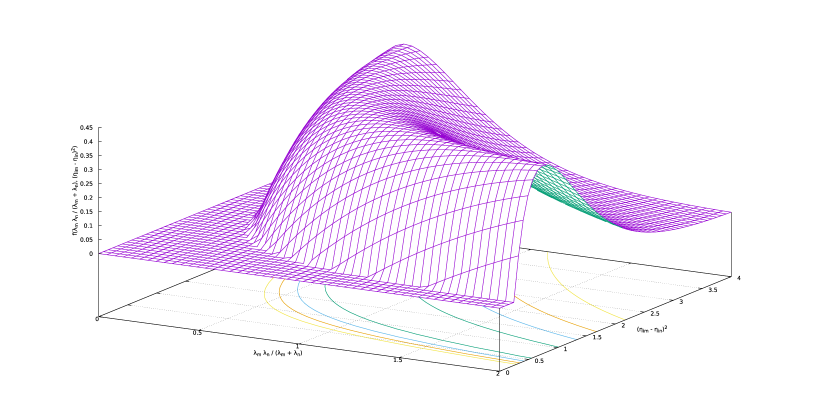
Figure 1: $f_{2}=\left[2\frac{\lambda_{m}\lambda_{n}}{\lambda_{m}+\lambda_{n}}(\eta_{im}-\eta_{in})^{2}-1\right]\exp\left\{-\frac{\lambda_{m}\lambda_{n}}{\lambda_{m}+\lambda_{n}}(\eta_{im}-\eta_{in})^{2}\right\}$

7.5 Operators

All the quantities of interest in the model described can be calculated, as happens in quantum mechanics, through the application of suitable operators. However, it must be taken into consideration that the values of the set of variational parameters $\Gamma$ obtained in the minimization of energy are not, in general, valid for other observables when using trial functions that are not the true eigenfunction of the system. This does not invalidate the results obtained in this section, in which we propose general expressions whose correctness in the numerical results is subject to the use of the correct values of the parameters $\Gamma$ for each observable under study.

7.5.1 Expected value for output $y_{k}$

Considering equation (15) and (19) we can write the following expression for the expected value of $y_{k}$

$$\left\langle y_{k}\right\rangle=\int y_{k}\left|\Psi\right|^{2}\,d\mathbf{x}=\sum_{p=1}^{P}\sum_{d=1}^{D}\sum_{l=1}^{D}w_{kp}c_{d}c_{l}\int\phi_{p}\psi_{d}\psi_{l}\,d\mathbf{x}+w_{k0}$$

Using equations (16) and (20) we obtain the final result

$$\begin{array}[]{rcl}\left\langle y_{k}\right\rangle&=&w_{k0}+\sum_{p=1}^{P}\sum_{d=1}^{D}\sum_{l=1}^{D}w_{kp}c_{d}c_{l}\left(\frac{\pi}{\xi_{p}+{\it\lambda}_{l}+{\it\lambda}_{d}}\right)^{\frac{N}{2}}\times\\ &&\prod_{i=1}^{N}\exp\left\{-\frac{\xi_{p}\left[\lambda_{l}\left({\it\omega}_{pi}-\eta_{il}\right)^{2}+{\it\lambda}_{d}\left({\it\omega}_{pi}-\eta_{id}\right)^{2}\right]+\lambda_{d}\lambda_{l}\left(\eta_{il}-\eta_{id}\right)^{2}}{\xi_{p}+{\it\lambda}_{l}+{\it\lambda}_{d}}\right\}\end{array}$$

7.5.2 Expected value for $x_{i}$

The expected value of a component $x_{i}$ of of the conditional probability $\left|\Psi(\mathbf{x})\right|^{2}$ is given by

$$\left\langle x_{i}\right\rangle=\int x_{i}\left|\Psi\right|^{2}\,d\mathbf{x}=\sum_{d=1}^{D}\sum_{l=1}^{D}c_{d}c_{l}\int x_{i}\psi_{d}\psi_{l}\,d\mathbf{x}$$

and using equations (16) and (20)

$$\left\langle x_{i}\right\rangle=\sum_{d=1}^{D}\sum_{l=1}^{D}c_{d}c_{l}\left(\lambda_{d}\eta_{id}+\lambda_{l}\eta_{il}\right)\frac{\pi^{\frac{N}{2}}}{\left(\lambda_{d}+\lambda_{l}\right)^{\frac{N+2}{2}}}\prod_{i=1}^{N}\exp\left\{-\frac{\lambda_{d}\lambda_{l}}{\lambda_{d}+\lambda_{l}}\left(\eta_{il}-\eta_{id}\right)^{2}\right\}$$

7.5.3 Expected value for the variance of $x_{i}$

Variance for $x_{i}$ is given by

$$(\Delta x_{i})^{2}=\left\langle x_{i}^{2}\right\rangle-\left\langle x_{i}\right\rangle^{2}$$

7.6 Uncertainty principle

In this section we make an analysis of the possible validity of the uncertainty principle within the EANNs. For simplicity we will consider in the treatment the one-dimensional case, that is a system composed by a neural network with a single input $x$.

From a direct comparison between the differential equation describing the physical behavior of the EANNs and the Schrõdinger equation, we postulate the following expression for the operator $\hat{p}_{x}^{2}$

$$\hat{p}_{x}^{2}=-\sigma_{x}^{2}\nabla^{2}$$ (50)

The negative sign allows to obtain positive kinetic energies, as has been confirmed by the experiments detailed in Section 8, and necessarily leads to an expression for momentum operator $\hat{p}_{x}$ which contains the imaginary unit

$$\hat{p}_{x}=\frac{\sigma_{x}}{i}\nabla$$ (51)

According to the laws of probability, the variances $\left(\Delta x\right)^{2}$ and $\left(\Delta p_{x}\right)^{2}$ related to the observables $x$ and $p_{x}$ can be written as [49]

$$\left(\Delta x\right)^{2}=\left\langle(x-\left\langle x\right\rangle)^{2}\right\rangle=\left\langle x^{2}\right\rangle-\left\langle x\right\rangle^{2}=\int\Psi^{*}(\hat{x}-\left\langle x\right\rangle)^{2}\Psi\,dx$$ (52)

$$\left(\Delta p_{x}\right)^{2}=\left\langle(p_{x}-\left\langle p_{x}\right\rangle)^{2}\right\rangle=\left\langle p_{x}^{2}\right\rangle-\left\langle p_{x}\right\rangle^{2}=\int\Psi^{*}(\hat{p}_{x}-\left\langle p_{x}\right\rangle)^{2}\Psi\,dx$$ (53)

Equations (52) and (53) are in fact definitions of a variance. In particular, the equation (52) is the expected value of the quadratic deviation of the variable $x$ measured against a conditional probability density given by the square of the state function, and should not be confused with $\sigma_{x}^{2}$, which is the variance given by the marginal probability density of $x$. Taking into account the definition of expected value and the mathematical properties of Schwartz’s inequality, for the product of standard deviations we have [14, 63]

$$\Delta x\Delta p_{x}\geq\frac{1}{2}\left|\int\Psi^{*}[\hat{x},\hat{p}_{x}]\Psi\,dx\right|$$ (54)

where $[\hat{x},\hat{p}_{x}]$ is the commutator for position, $\hat{x}$, and momentum, $\hat{p}_{x}$, operators.

If we consider valid the rules of commutation in quantum mechanics and their meaning as the possibility or not of measuring with arbitrary precision the values of conjugated variables, then there exits an uncertainty relationship also in the EANNs. The reason lies in the fact that any operator composed of a first derivative does not commute with the position operator. By defining the operator $\hat{D}=\frac{d}{dx}$, the commutator with $\hat{x}$ gives rise, as is known, to

$$\hat{D}\hat{x}=\hat{1}+\hat{x}\hat{D}$$

$$\left[\frac{d}{dx},\hat{x}\right]=\hat{D}\hat{x}-\hat{x}\hat{D}=\hat{1}$$

where $\hat{1}$ is the unit operator. In our case, for the position-momentum commutator, taking into account that $\left[\hat{x},\hat{p}_{x}\right]=-\left[\hat{p}_{x},\hat{x}\right]$, we have

$$\left[\hat{x},\hat{p}_{x}\right]=\left[\hat{x},\frac{\sigma_{x}}{i}\frac{\partial}{\partial x}\right]=\frac{\sigma_{x}}{i}\left[\hat{x},\frac{\partial}{\partial x}\right]=-\frac{\sigma_{x}}{i}\left[\frac{\partial}{\partial x},\hat{x}\right]=-\frac{\sigma_{x}}{i}=i\sigma_{x}$$

Finally, from the equation (54)

$$\Delta x\Delta p_{x}\geq\frac{1}{2}\left|\int\Psi^{*}i\sigma_{x}\Psi\,dx\right|=\frac{\sigma_{x}}{2}\left|i\right|\left|\int\Psi^{*}\Psi\,dx\right|$$

$$\Delta x\Delta p_{x}\geq\frac{\sigma_{x}}{2}$$ (55)

Assuming therefore an operator of the form (51) and taking into account very general considerations, we obtain an equivalent of the uncertainty principle for the EANNs. This result is not surprising given the mathematical equivalence with the Schrõdinger equation.

It is possible to generalize this result for pairs of generic conjugated variables if one assumes the validity for the EANN of some classical results in quantum mechanics, which however needs formal verification. If the equation (18) governs the behavior of a true quantum system in which not all pairs of variables commute, we can hypothesize the existence of a classic system in which all variables instead commute. In this context, from a quantum point of view an equivalent of Dirac’s proposal for pairs of variables $(f,g)$ is

$$[\hat{f},\hat{g}]=i\sigma_{x}\left\{f,g\right\}$$

where $\left\{f,g\right\}$ is the Poisson bracket between $f$ and $g$.

From a physical point of view, the equation (54) is a formalization of the impossibility of simultaneously measuring position and momentum with arbitrary precision, ie the fact that the variance in the position is subject to a kinematic constraint [6]. Equivalently, within non-commutative algebras, it makes explicit the fact that position and momentum cannot be made independent from a statistical point of view, constituting a limit to a priori knowledge regarding observable statistics and their predictability. Equation (55) highlights how the product in the uncertainties or variances of two non-independent observables cannot be less than a certain minimum value, which is related to the standard deviation of the marginal density of the dataset.

Equation (55) can be derived from purely statistical considerations. Starting from the inequality proposed independently by Bourret [12], Everett [22], Hirschman [41] and Leipnick [48], satisfied by each function $\psi$ and its Fourier transform $\widetilde{\psi}$

$$-\int\left|\psi(x)\right|^{2}\ln\left|\psi(x)\right|^{2}\,dx-\int\left|\widetilde{\psi}(p_{x})\right|^{2}\ln\left|\widetilde{\psi}(p_{x})\right|^{2}\,dp_{x}=h(x)+h(p_{x})\geq 1+\ln\pi$$

Beckner [7] and Bialinicki-Birula and Micielski [10] demonstrated

$$h(x)+h(p_{x})\geq\ln(\pi e\sigma_{x})$$ (56)

where we assumed the equivalence $\hbar\equiv\sigma_{x}$. Since the differential entropy of the normal probability density is maximum among all distributions with the same variance, for a generic probability density $f(z)$ we can write the inequality

$$h(z)\leq\ln(\sqrt{2\pi e}\Delta z)$$ (57)

Substituting (57) in (56) we have

$$\Delta x\Delta p\geq\frac{1}{2\pi e}\exp\left\{h(x)+h(p_{x})\right\}\geq\frac{\sigma_{x}}{2}$$

It is worth mentioning that the equation (56) is derived from mathematical properties and acquires the form of the text at the end of the proof, when considering a concrete expression for $p_{x}$.

Finally, the uncertainty principle can also be derived from the Cramér-Rao bound, as demonstrated by several authors [2, 21, 31, 35, 34, 39, 58, 64, 71], that is, starting from exclusively statistical properties. Section 2 contains the bibliographic references of some significant works related to this topic.

7.7 Time-dependent system

The discussion of previous sections has considered stationary systems. Independence from time, as we have highlighted, is based on the temporal invariance of the set of constants $\vec{\rho},\vec{\theta},\vec{\mu}$ and $\vec{\sigma}$ which identify the problem. However, given a dataset, it is reasonable to assume its temporal evolution, identified as the acquisition of new data that vary $\vec{\rho},\vec{\theta},\vec{\mu}$ and $\vec{\sigma}$ between an initial state and a final state. In the following we will consider for simplicity the one-dimensional case ($N=1$).

We postulate the following expression for a time-dependent system

$$\begin{array}[]{rcl}-\frac{\mathcal{A}}{i}\frac{d\Psi(x,\tau)}{d\tau}&=&-\frac{\sigma_{x}^{2}(x,\tau)}{(2\pi)^{1/2}\left|\Sigma(x,\tau)\right|^{1/2}}\nabla^{2}\Psi(x,\tau)+\mathcal{N}(x,\tau)\times\\ &&\sum_{k=1}^{C}\left[\alpha_{k}(x,\tau)y_{k}^{2}(x,\tau)+\beta_{k}(x,\tau)y_{k}(x,\tau)+\gamma_{k}(x,\tau)\right]\Psi(x,\tau)\end{array}$$ (58)

where $\tau$ is time, $\mathcal{A}$ is a factor to be determined and where we have explicitly highlighted the temporal dependence of all terms. In this version, the values of $\vec{\rho},\vec{\theta},\vec{\mu}$ and $\vec{\sigma}$ and the weights of the network are generally different in the initial and final states and therefore depend on time in a way, however, that we don’t know. This also implies a temporal evolution in the marginal densities $p(x)$ and $p(t)$. To make matters worse than quantum physical systems that have time-dependent potentials, the equation (58) also contains a time-dependent factor for the kinetic term ($\sigma,\Sigma)$. Furthermore, in the absence of explicit expressions, the time functional factors introduce dimensional problems in the equation (58). In practice, given the lack of knowledge of the functional dependence on time of the terms that appear on the right hand side of the equation (58), we can consider it as not solvable. Imaginary unit in the left hand side is necessary if we consider certain conditions met, as we will see later in the discussion. Term $-\frac{\mathcal{A}}{i}\frac{d\Psi}{d\tau}$ can be seen as the result of a Wick rotation of $\mathcal{A}\frac{d\Psi}{d\tau_{w}}$ in time $\tau_{w}=-i\tau$.

Systems with time-dependent potentials are approached in quantum mechanics, in many cases, with a Hamiltonian consisting of two terms: one time-independent and one time-dependent, the last being treated as a perturbation

$$H(x,\tau)=H_{0}(x)+V(x,\tau)$$

where $H_{0}(x)$ is the Hamiltonian of the equation (18). Supposing that $V(x,\tau)$ is negligible compared to $H_{0}(x)$, equation (58) becomes

$$-\frac{\mathcal{A}}{i}\frac{d\Psi}{d\tau}=-\frac{\sigma_{x}^{2}}{(2\pi)^{1/2}\left|\Sigma\right|^{1/2}}\nabla^{2}\Psi+\mathcal{N}(\mu,\sigma_{x}^{2})\sum_{k=1}^{C}(\alpha_{k}y_{k}^{2}+\beta_{k}y_{k}+\gamma_{k})\Psi$$ (59)

The right hand side has units given by the factor $\frac{1}{\left|\Sigma\right|^{1/2}}$ and must be introduced in the left hand side to maintain dimensional consistency. However, the differential equation governing an EANN does not contain any time-dependent constant factor, unlike what happens with the constant $\hbar$ in the time-dependent version of the Schrõdinger equation. The dimensional coherence between the two members of the equation (59) imposes the following expression for $\mathcal{A}$

$$\mathcal{A}=\frac{\tau}{\left|\Sigma\right|^{1/2}}$$

Assuming a solution given in the form

$$\Psi(x,\tau)=f(\tau)\psi(x)$$

equation (59) becomes separable, being the parts time-dependent and time-independent equal to a constant that can be shown is the system energy. For the time-dependent part we have the following ordinary differential equation

$$\frac{df(\tau)}{f(\tau)}=-\frac{i\left|\Sigma\right|^{1/2}E}{\tau}\,d\tau$$

whose solution is

$$f(\tau)=\tau^{-i\left|\Sigma\right|^{1/2}E}=\exp\left\{-i\left|\Sigma\right|^{1/2}E\ln(\tau)\right\}$$ (60)

where the integration constant has been omitted since it can be included as a factor in the $\psi(x)$ function. The last equality of equation (60) expresses a periodic function in the variable $\tau^{\prime}=\ln(\tau)$.

We now justify the presence of the imaginary unit in the equation (60). Following quantum mechanics, we impose the condition that for a pure eigenfunction $\Psi(x,\tau)$ the probability density is stationary [49]

$$\left|\Psi(x,\tau)\right|^{2}=\left|\psi(x)\right|^{2}$$

Mathematically, this condition leads to

$$f^{*}(\tau)f(\tau)=1$$ (61)

which can only be satisfied if $f(\tau)$ is a complex function. More formally, it is possible to define an operator $\hat{U}(\tau,\tau_{0})$ that describes the temporal evolution of the system according to the equation

$$-\frac{\tau}{i\left|\Sigma\right|^{1/2}}\frac{d}{d\tau}\hat{U}(\tau,\tau_{0})=\hat{H}\hat{U}(\tau,\tau_{0})$$

subject to the initial condition

$$\hat{U}(\tau_{0},\tau_{0})=1$$

Equality (61) expresses the unitarity of $\hat{U}$, a property derived from the hermiticity of $\hat{H}$ [54].

As is known, the probability density is not stationary for a system that makes a temporal transition from a state $m$ to a state $n$. The state function of this system can be written as a linear combination of the two states

$$\Psi_{mn}(x,\tau)=c_{m}\Psi_{m}(x,\tau)+c_{n}\Psi_{n}(x,\tau)$$

If $(c_{m},c_{n})\neq 0$, the probability density is

$$\left|\Psi_{mn}\right|^{2}=c_{m}^{2}\left|\Psi_{m}\right|^{2}+c_{n}^{2}\left|\Psi_{n}\right|^{2}+c_{m}c_{n}(\Psi_{m}^{*}\Psi_{n}+\Psi_{m}\Psi_{n}^{*})$$

The first two terms of the right hand side are time-independent. By developing the calculation and considering, as we did in this paper, only real functions for the time-independent component of the state function, the final time-dependent probability density is

$$\left|\Psi_{mn}\right|^{2}=c_{m}^{2}\psi_{m}^{2}+c_{n}^{2}\psi_{m}^{2}+2c_{m}c_{n}\psi_{m}\psi_{n}\cos\left\{\left(\left|\Sigma_{m}\right|^{1/2}E_{m}-\left|\Sigma_{n}\right|^{1/2}E_{n}\right)\tau^{\prime}\right\}$$ (62)

Equation (62) expresses the evolution of the conditional probability density $\Psi(x,\tau|\mathbf{t})$ between two states separated in time. The state function consisting of a mixture of two energy states does lead to a conditional density that oscillates in the logarithmic time $\tau^{\prime}$ with frequency

$$\nu=\left|\Sigma_{m}\right|^{1/2}E_{m}-\left|\Sigma_{n}\right|^{1/2}E_{n}$$

8 Results

The resolution of the system (25) requires considerable computational powers. For this reason the minimum energy was calculated with a genetic algorithm (GA).

The test problem comes from the Statlib repository. It is a synthetic dataset made up of 3848 records, generated by David Coleman, referred to for convenience as POLLEN, which represents geometric and physical characteristics of pollen grain samples. It consists of 5 variables: the first three are the lengths in the directions x (ridge), y (nub) and z (crack), the fourth is the weight and the fifth is the density, the latter being the target of the problem. In our model they represent, respectively, $x_{1}$, $x_{2}$, $x_{3}$, $x_{4}$ and $t_{1}$. The choice of this problem lies in the fact that the data were generated with normal distributions with low correlations, and is therefore close to the initial assumptions of the model for $\mathbf{x}$ and $\mathbf{t}$. Tables 2 and 3 show the general statistics of the dataset.

Table 2: POLLEN dataset, general features. The table shows the means ($\mu$, $\rho$), standard deviations ($\sigma$, $\theta$), skewness and kurtosis (the reference for normality is 0) of original and normalized data

	Original data		Normalized data		Skewness	Kurtosis
Var	$\mu$ / $\rho$	$\sigma$ / $\theta$	$\mu$ / $\rho$	$\sigma$ / $\theta$
$x_{1}$	-3.637e-03	6.398	0.0418	0.2863	-0.130	-0.057
$x_{2}$	1.597e-04	5.186	-0.0257	0.3082	0.072	-0.311
$x_{3}$	3.103e-03	7.875	0.0178	0.2551	-0.057	-0.158
$x_{4}$	4.237e-03	10.004	-0.0252	0.2876	0.109	-0.163
$t_{1}$	1.662e-04	3.144	0.0512	0.2745	0.110	0.192

Table 3: Dataset POLLEN, correlation matrix

	$x_{1}$	$x_{2}$	$x_{3}$	$x_{4}$	$t_{1}$
$x_{1}$	1.00	0.13	-0.13	-0.90	-0.57
$x_{2}$	0.13	1.00	0.08	-0.17	0.33
$x_{3}$	-0.13	0.08	1.00	0.27	-0.15
$x_{4}$	-0.90	-0.17	0.27	1.00	0.24
$t_{1}$	-0.57	0.33	-0.15	0.24	1.00

The characteristics of the genetic algorithm have been described in a previous paper [5]. This is a steady-state GA, with a generation gap of one or two, depending on the operator applied. The population has binary coding and implements a fitness sharing mechanism [32] to allow speciation and avoid premature convergence, according to the equations

$$E_{l}^{{}^{\prime}}=E_{l}\sum_{m}\varphi(d_{lm})$$ (63)

$$\varphi(d_{lm})=\left\{\begin{array}[]{lcr}1-\left(\frac{d_{lm}}{R}\right)^{\upsilon}&\Rightarrow&d_{kl}<R\\ 0&\Rightarrow&d_{kl}\geq R\end{array}\right.$$

being $\varphi(d_{lm})$ a function of the diversity between individuals $l$ and $m$, $d_{lm}$ the Hamming distance and $R$ the niche radius within which individuals are considered similar. Niche sharing implements a correction to energy calculated based on the similarity between the individual $l$ and the rest of the population. The more similar it is, the greater the value of $\varphi(d_{lm})$, penalizing the energy in the equation (63) since we are minimizing.

The decoding of the genotype implements the Gray code to avoid discontinuities in the binary representation. The transformation between the binary representations, $b$, and Gray, $g$, for the $i$-th bit, considering numbers composed of $n$ bits numbered from right to left, with the most significant bit on the left, is given by

$$\begin{array}[]{c}g_{i}=\left\{\begin{array}[]{ccl}b_{i}&\Rightarrow&i=n\\ b_{i+1}\otimes b_{i}&\Rightarrow&i<n\end{array}\right.\\ b_{i}=\left\{\begin{array}[]{ccl}g_{i}&\Rightarrow&i=n\\ b_{i+1}\otimes g_{i}&\Rightarrow&i<n\end{array}\right.\end{array}$$

where $\otimes$ is the XOR operator.

The GA uses four operators: crossover, mutation, uniform crossover and internal crossover, and performs a search in the space of the computed energies according to the equation (24), but simultaneously realizes a search in the space of the operators through the use of two additional bits in the genotype of each individual of the population. This allows a dynamic choice of the probabilities of each operator at each moment of the calculation, according to the fraction of elements of the population that were generated and encode for each of the four possibilities. The initial population is randomly generated.

The procedure for assessing an individual consists of the following steps:

1. the values of the $n_{\Gamma}$ parameters are generated within certain prefixed ranges through the application of one of the operators;

2. the network output, $y_{k}$, is generated for each element of the dataset. This set of values allows to calculate $\chi_{k}$;

3. the $D\times D$ elements of the matrices $\mathbf{H}$ and $\mathbf{S}$ are computed by means of the integrals (26) and (27);

4. the determinant (28) is calculated;

5. the system (25) is solved.

Result is the $D$ energy values, $E_{d}$, and the $D$ coefficients $c$ for each of the $D$ state functions $\Psi_{d}$. The lower value among $E_{d}$ represents the global optimum of the problem.

Before the execution of the tests, a preprocessing of the dataset was performed, normalizing $\mathbf{x}$ and $t$ within the range $\Delta\equiv[-1:1]$. 15 calculations were conducted, each consisting of 10 concurrent processes sharing the best solution found. In each calculation the set of lower energy solutions found in the previous calculations were introduced. The values of the $n_{\Gamma}$ parameters were varied within certain pre-established ranges, identified through a preliminary test campaign. The reference ranges are shown in Table 4. Table 5 shows the reference values of the parameters used in the genetic algorithm.

Table 4: Values of the model and range of variability of the $n_{\Gamma}$ variational parameters, and $\mathbf{x}$ and $t_{1}$ data of the dataset

Variable	Value
C	1
D	12
N	4
P	20
$\mathbf{x},t_{1}$	$[-1:1]$
$\lambda,\xi$	$[0:4]$
w	$[-4:4]$
$\eta,\omega$	$[-1:1]$

Table 5: Reference values of the genetic algorithm

Variable	Value
Population	250
Point mutation probability	$[0:0.01]$
$\upsilon$	1
Chromosome length	3877 bits
Calculation cycles	20000

Results of the genetic algorithm for the parameters of basis functions $\phi$ of the network $y_{k}$

$\xi$	P \ N	$\omega_{1}$	$\omega_{2}$	$\omega_{3}$	$\omega_{4}$
2.919328e+00	$\omega_{1}$	-9.616850e-01	5.699350e-01	-1.007076e-01	8.523940e-01
8.423300e-01	$\omega_{2}$	9.177860e-01	1.001960e-01	7.096600e-01	4.823590e-01
2.087150e-01	$\omega_{3}$	-2.578000e-01	5.203320e-01	-8.117540e-01	-8.377960e-01
3.914241e+00	$\omega_{4}$	-3.191230e-01	4.871910e-01	-8.830230e-01	5.089810e-01
5.823370e-01	$\omega_{5}$	-6.928290e-01	2.672930e-01	-4.297810e-01	-3.016050e-01
1.926436e+00	$\omega_{6}$	-8.767050e-01	-3.759150e-01	-9.127510e-01	9.698310e-01
3.097580e-01	$\omega_{7}$	-5.724300e-01	9.825380e-01	-6.680690e-01	9.482790e-01
3.858523e+00	$\omega_{8}$	2.538800e-01	8.884770e-01	8.543280e-01	5.800880e-01
2.705241e+00	$\omega_{9}$	-7.541110e-01	-1.327950e-01	-5.627170e-01	9.081580e-01
9.479430e-01	$\omega_{10}$	-6.158020e-01	1.714950e-01	-9.497280e-01	9.030120e-01
1.103653e+00	$\omega_{11}$	-4.964920e-01	1.040151e-01	-9.430600e-01	3.068200e-01
3.384321e+00	$\omega_{12}$	6.543940e-01	-9.356290e-01	4.894600e-01	7.890730e-01
7.454340e-01	$\omega_{13}$	-8.030510e-01	-2.275000e-01	-4.027400e-01	-5.026880e-01
1.926320e+00	$\omega_{14}$	-5.985470e-01	1.618350e-01	-8.644710e-01	-2.648060e-01
1.349549e+00	$\omega_{15}$	-2.659290e-01	-4.931090e-01	7.594300e-01	1.028353e-01
2.424388e+00	$\omega_{16}$	5.962460e-01	6.320610e-01	-4.129300e-01	-5.073280e-01
6.307950e-01	$\omega_{17}$	-4.769380e-01	8.363110e-01	2.817150e-01	1.914970e-01
2.245460e-01	$\omega_{18}$	5.409380e-01	7.000500e-01	9.406210e-01	-3.607610e-01
3.103390e+00	$\omega_{19}$	-1.407570e-01	-1.708480e-01	-3.897940e-01	1.832320e-01
2.451465e+00	$\omega_{20}$	-9.182390e-01	3.936930e-01	3.930220e-01	4.795600e-01

Table 6: Results of the genetic algorithm for network weights

P \ C	$w_{1}$
$w_{0}$	1.638795e+00
$w_{1}$	1.419237e+00
$w_{2}$	-1.858620e+00
$w_{3}$	-2.603692e+00
$w_{4}$	1.118712e+00
$w_{5}$	1.239672e+00
$w_{6}$	-1.197724e+00
$w_{7}$	-1.490210e+00
$w_{8}$	1.755702e+00
$w_{9}$	9.814800e-01
$w_{10}$	-2.964685e+00
$w_{11}$	2.344582e+00
$w_{12}$	-1.652975e+00
$w_{13}$	3.030500e-01
$w_{14}$	-6.988870e-01
$w_{15}$	-3.270600e-01
$w_{16}$	5.944650e-01
$w_{17}$	1.834500e+00
$w_{18}$	-5.652970e-01
$w_{19}$	-1.576270e-01
$w_{20}$	-9.845600e-01

Results of the genetic algorithm for the coefficients and parameters of basis functions $\psi_{d}$ of the state function $\Psi$

$c$	$\lambda$	P \ N	$\eta_{1}$	$\eta_{2}$	$\eta_{3}$	$\eta_{4}$
1.553121e+00	1.390160e-01	$\eta_{1}$	-1.231300e-01	-4.406100e-01	-2.818570e-01	2.351560e-01
-2.359102e-01	1.925760e-01	$\eta_{2}$	-1.194100e-01	1.004575e-01	-1.022693e-01	1.308700e-01
-1.904793e+00	1.085620e-01	$\eta_{3}$	8.793090e-01	4.690850e-01	-3.208850e-01	1.048543e-01
-2.639326e+00	1.093980e-01	$\eta_{4}$	-4.300890e-01	-4.877940e-01	-1.046653e-01	2.051050e-01
2.014761e-01	1.000033e-01	$\eta_{5}$	-8.999490e-01	1.039123e-01	-4.522900e-01	4.788520e-01
1.682093e-01	1.394260e-01	$\eta_{6}$	-7.989670e-01	1.157740e-01	4.029300e-01	-1.007880e-01
-2.765379e-01	1.799000e-01	$\eta_{7}$	1.007745e-01	-6.873660e-01	-4.912310e-01	2.924720e-01
9.654897e-01	1.000023e-01	$\eta_{8}$	-5.837550e-01	-7.069950e-01	1.034500e-01	3.353310e-01
4.245192e-01	1.382240e-01	$\eta_{9}$	9.013570e-01	6.677700e-01	-2.735550e-01	1.025390e-01
8.729764e-01	1.000193e-01	$\eta_{10}$	9.922380e-01	4.842470e-01	-4.106250e-01	2.306550e-01
1.726046e-01	1.000000e-01	$\eta_{11}$	-7.864230e-01	-9.010480e-01	-5.281260e-01	-4.112000e-01
7.787302e-01	1.000035e-01	$\eta_{12}$	5.929010e-01	2.620350e-01	-1.567570e-01	-1.024260e-01

Table 7: Results of the genetic algorithm for the network $y_{k}$ with lower energy

Calculation	Variable	Value
Train	$\alpha_{1}$	6.504147
	$\beta_{1}$	-7.050345e-01
	$\gamma_{1}$	1.776158e-01
	$\chi_{1}$	1.752492e-01
	$E_{r}$	0.768%
	$E$	5.969894e-02 enats
	$\left\langle T\right\rangle$	5.944988e-02 enats
	$\left\langle V\right\rangle$	2.490563e-04 enats
	$W$	2.772339 enats
	$\mathcal{C}$	8.982000e-05
Test	$\alpha_{1}$	7.058333
	$\beta_{1}$	-5.941080e-01
	$\gamma_{1}$	1.418035e-01
	$\chi_{1}$	1.769226e-01
	$E_{r}$	0.782%
	$E$	5.989879e-02 enats
	$\left\langle T\right\rangle$	5.964383e-02 enats
	$\left\langle V\right\rangle$	2.549622e-04 enats
	$W$	2.772333 enats
	$\mathcal{C}$	9.194974e-05

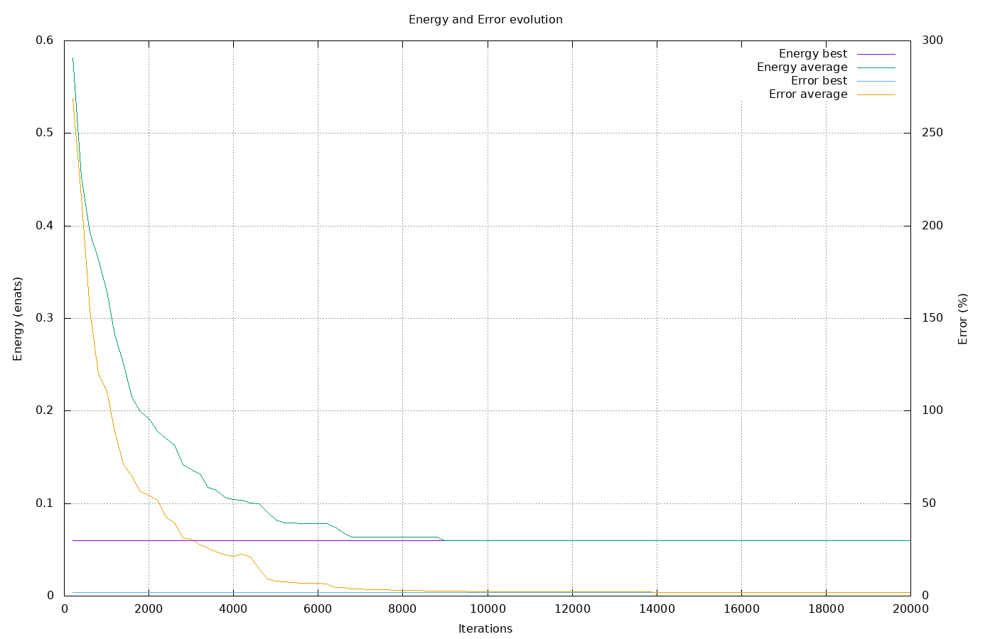
Figure 2: Evolution of the genetic algorithm that produced the solution with lower energy for the dataset POLLEN. Average and better (lower) energy and error decrease with the number of generations of the GA.

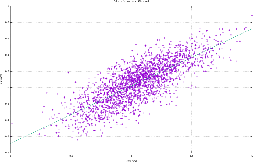
Figure 3: Dispersion plot for the POLLEN problem of calculated data generated by the optimal neural network vs. observed data (dataset) for the training partition.

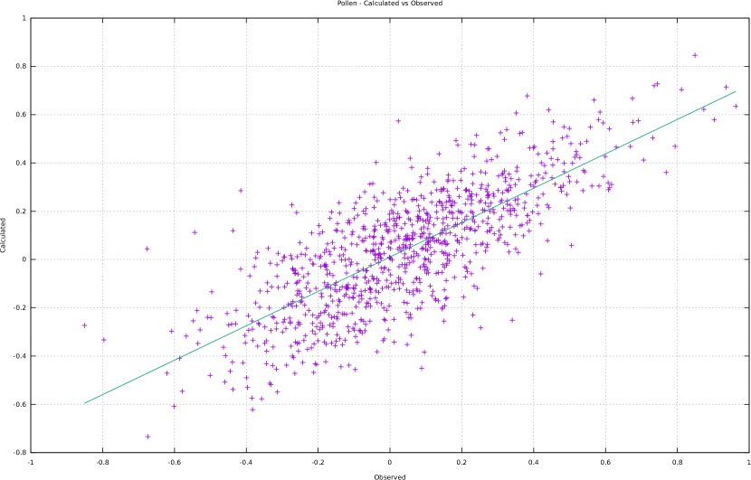
Figure 4: Dispersion plot for the POLLEN problem of calculated data generated by the optimal neural network vs. observed data (dataset) for the testing partition.

For each element of the population, in addition to the energy value, has been calculated the square error percentage of the neural network [5, 61]

$$E_{r}=\frac{100}{s(t_{max}-t_{min})^{2}}\sum_{s}(y_{s}-t_{s})^{2}$$

where $s$ is the number of records in the dataset and $t_{max}-t_{min}=2$ depends on the normalization interval used.

Some of the parameters in the Table 5 deserve some observation:

• $\upsilon=1$ implies the so-called triangular niche sharing;

• $R$ has a considerable influence on the results and was chosen for each of the 10 concurrent processes of each calculation according to the criterion $R_{i}=(i-1)/10,\,i=1,\ldots,10$, where $i$ is the process number. This allows to avoid arbitrary choices since $R$ can be dependent on the nature of the problem;

• $\xi$ was chosen in the interval $[0:4]$, which includes the value given by a heuristic RBF rule which proposes for the standard deviation of the associated normal distribution, $\sigma_{\xi}=\sqrt{\frac{1}{2\xi}}$, the reference value $2\bar{d}_{\omega}$, where $\bar{d}_{\omega}$ is the average value between the centroids of the functions $\phi_{p}$ of the equation (16). Considering an estimate of $\bar{d}_{\omega}=1$ (half of the normalization interval) we get $\xi=0.125$. The range $\xi\in[0:4]$ is equivalent to $\sigma_{\xi}\in[0.354:\infty]$. The same criterion has also been used for the vector $\vec{\lambda}$.

The dataset was divided into two parts, a set of training (2886 records) and a set of testing (962 records). Technically this subdivision is not necessary, since the two data partitions are generated by the same distribution and the characterization of the problem in the model is given exclusively by the value of the constants $\vec{\rho}$, $\vec{\theta}$, $\vec{\mu}$ and $\vec{\sigma}$, which are almost the same for both partitions.

The variational parameters of the best solution are reported in Tables 8, 6 and 8. The final results of the calculation, including error and energy, are shown in Table 7. Figure 2 shows the evolution of error and energy (lower and average) of the calculation that generated the lower energy solution, which shows how the minimization of energy leads to a decrease of the error committed by the net in the target prediction. The final error value for training (0.768%) and testing (0.782%) partitions is particularly significant given the low number of basis functions used in the definition of $\Psi$ and $y_{k}$. Figures 3 and 4 show the dispersion graphs of the network output vs. observed values for the target (dataset) generated by the optimal net.

9 Conclusions

In this work we have developed a model for optimizing artificial neural networks based on an analogy with a physical quantum-mechanical system using a potential based on the MinMI principle. This principle has the sense to identify an approximation to the true relationship between inputs and targets, stripping it of unnecessary superstructures. With regard to the model that we have proposed, the starting point of this paper is made from the observation of some analogies that lead to treat the problem of the optimization of a neural network as a physical system governed by an eigenvalue equation, taken without justification, and to develop the consequences of such an approach.

The author took a lot of freedom in the initial setting of this work. However, the quality of the results obtained in applying the model to a series of problems (only one of these tests is reported in this paper) prompted us to formalize the model and give it adequate mathematical consistency. It is possible to deepen further the formal bases on some of the topics treated and the mathematical expressions obtained, many of which are postulated on the basis of simple dimensional analysis of the equations. Extending the potential applicability of the formalism and the results of quantum mechanics to the EANNs requires a separate study that is outside the scope of this paper. Such a study is desirable given the encouraging results obtained.

We underline some particular points of interest of this work:

1. The possibility of using, in the study of neural networks, the results of a theory, quantum mechanics, with a high degree of mathematical and conceptual maturity.

2. The potential possibility of applying the model to a wide variety of problems, in particular those not covered in this paper, such as datasets with discrete inputs/outputs and time series.

3. The fact that it is possible to realize the optimization of a neural network for a problem by solving the system of linear equations (30), allowing in principle to obtain the solution with a deterministic procedure in real time. If the system (30) is calculable, then a training process intended in the sense of conventional procedures such as backpropagation is not necessary. The potential possibility of decrease the calculation times represents a point of interest.

4. Results for the POLLEN problem is particularly significant, given the low final errors in the prediction of the dataset, obtained with a very low number of basis functions in the definition of $\Psi$ and $y_{k}$.

It is necessary to carry out a systematic test campaign to verify the results obtained. These tests are currently underway and will be the subject of a subsequent work. The preliminary results obtained on a set of selected problems coming from the Statlib and UCI repositories confirm the validity of the model. Prediction errors calculated with optimized EANNs are of the same order of magnitude as those obtained with conventional techniques: genetic algorithms, simulated annealing and backpropagation.

References

- del [2012] Information theory: new research. In Pierre Deloumeaux and Jose D. Gorzalka, editors, Information theory: new research, Mathematics research developments. Nova Science Publishers, New York, 2012. ISBN 978-1-62100-325-0.
- Angelow [2009] Andrew Angelow. Evolution of Schrödinger Uncertainty Relation in Quantum Mechanics. NeuroQuantology, 7(2), February 2009. ISSN 13035150. doi: 10.14704/nq.2009.7.2.235.
- Baran et al. [2001] B. Baran, J. Vallejos, R. Ramos, and U. Fernandez. Multi-objective reactive power compensation. In 2001 IEEE/PES Transmission and Distribution Conference and Exposition. Developing New Perspectives (Cat. No.01CH37294), volume 1, pages 97–101, Atlanta, GA, USA, 2001. IEEE. ISBN 978-0-7803-7285-6. doi: 10.1109/TDC.2001.971215.
- Baran et al. [2017] Turkay Baran, Nilgun B. Harmancioglu, Cem Polat Cetinkaya, and Filiz Barbaros. An Extension to the Revised Approach in the Assessment of Informational Entropy. Entropy, 19(12):634, December 2017. doi: 10.3390/e19120634.
- Barrera [2007] Francisco Yepes Barrera. Búsqueda de la estructura óptima de redes neurales con algoritmos genéticos y simulated annealing. verificación con el benchmark proben1. Inteligencia Artificial, Revista Iberoamericana de IA, 11(34):41–61, 2007.
- Bastos et al. [2015] Catarina Bastos, Alex E Bernardini, Orfeu Bertolami, Nuno Costa Dias, and João Nuno Prata. Robertson-Schrödinger formulation of Ozawa’s uncertainty principle. Journal of Physics: Conference Series, 626:012050, July 2015. ISSN 1742-6588, 1742-6596. doi: 10.1088/1742-6596/626/1/012050.
- Beckner [1975] William Beckner. Inequalities in Fourier Analysis. The Annals of Mathematics, 102(1):159, July 1975. ISSN 0003486X. doi: 10.2307/1970980.
- Benoudjit and Verleysen [2003] Nabil Benoudjit and Michel Verleysen. On the Kernel Widths in Radial-Basis Function Networks. Neural Processing Letters, 18:139–154, 2003.
- Benoudjit et al. [2002] Nabil Benoudjit, Cédric Archambeau, Amaury Lendasse, John Lee, and Michel Verleysen. Width optimization of the Gaussian kernels in Radial Basis Function Networks. In ESANN 2002 proceedings - European Symposium on Artificial Neural Networks, pages 425–432, Belgium, 2002. ISBN 2-930307-02-1.
- Bialynicki-Birula and Mycielski [1975] Iwo Bialynicki-Birula and Jerzy Mycielski. Uncertainty relations for information entropy in wave mechanics. Communications in Mathematical Physics, 44(2):129–132, June 1975. ISSN 0010-3616, 1432-0916. doi: 10.1007/BF01608825.
- Bishop [1995] Christopher M. Bishop. Neural Networks for Pattern Recognition. Oxford University Press, 1995.
- Bourret [1958] Richard Bourret. A note on an information theoretic form of the uncertainty principle. Information and Control, 1(4):398–401, December 1958. ISSN 00199958. doi: 10.1016/S0019-9958(58)90249-3.
- Braunstein and Caves [1990] Samuel L Braunstein and Carlton M Caves. Wringing out better Bell inequalities. Annals of Physics, 202(1):22–56, August 1990. ISSN 0003-4916. doi: 10.1016/0003-4916(90)90339-P.
- Briggs [2008] J S Briggs. A derivation of the time-energy uncertainty relation. Journal of Physics: Conference Series, 99:012002, February 2008. ISSN 1742-6596. doi: 10.1088/1742-6596/99/1/012002.
- Cerf and Adami [1997] N. J. Cerf and C. Adami. Entropic Bell Inequalities. Physical Review A, 55(5):3371–3374, May 1997. ISSN 1050-2947, 1094-1622. doi: 10.1103/PhysRevA.55.3371.
- Chen et al. [2008] Badong Chen, Jinchun Hu, Hongbo Li, and Zengqi Sun. Adaptive FIR Filtering under Minimum Error/Input Information Criterion. IFAC Proceedings Volumes, 41(2):3539–3543, 2008. ISSN 14746670. doi: 10.3182/20080706-5-KR-1001.00598.
- Chen et al. [2013] Badong Chen, Yu Zhu, Jinchun Hu, and Jose C. Principe. System Identification Based on Mutual Information Criteria. In System Parameter Identification, pages 205–238. Elsevier, 2013. ISBN 978-0-12-404574-3. doi: 10.1016/B978-0-12-404574-3.00006-3.
- Chern [2017] Albert Ren-Haur Chern. Fluid Dynamics with Incompressible Schrödinger Flow. phd, California Institute of Technology, 2017.
- Coles et al. [2017] Patrick J. Coles, Mario Berta, Marco Tomamichel, and Stephanie Wehner. Entropic Uncertainty Relations and their Applications. Reviews of Modern Physics, 89(1):015002, February 2017. ISSN 0034-6861, 1539-0756. doi: 10.1103/RevModPhys.89.015002.
- Contreras et al. [2010] Mauricio Contreras, Rely Pellicer, Marcelo Villena, and Aaron Ruiz. A quantum model of option pricing: When Black-Scholes meets Schrödinger and its semi-classical limit. Physica A: Statistical Mechanics and its Applications, 389(23):5447–5459, December 2010. ISSN 03784371. doi: 10.1016/j.physa.2010.08.018.
- Dembo et al. [1991] A. Dembo, T.M. Cover, and J.A. Thomas. Information theoretic inequalities. IEEE Transactions on Information Theory, 37(6):1501–1518, November 1991. ISSN 1557-9654. doi: 10.1109/18.104312.
- DeWitt et al. [1973] Bryce S. DeWitt, Hugh Everett, and Neill Graham. The many-worlds interpretation of quantum mechanics: a fundamental exposition. Princeton series in physics. Princeton University Press, Princeton, N.J, 1973. ISBN 978-0-691-08126-7 978-0-691-08131-1.
- Falaye et al. [2016] B. J. Falaye, F. A. Serrano, and Shi-Hai Dong. Fisher’s information for the position-dependent mass Schrödinger system. Physics Letters A, 380(1-2):267–271, January 2016. ISSN 03759601. doi: 10.1016/j.physleta.2015.09.029.
- Feldman and Crutchfield [1997] David P. Feldman and James P. Crutchfield. Statistical Measures of Complexity: Why? arXiv:cond-mat/9708186, August 1997. arXiv: cond-mat/9708186.
- Fernández et al. [2013] Nelson Fernández, Carlos Maldonado, and Carlos Gershenson. Information Measures of Complexity, Emergence, Self-organization, Homeostasis, and Autopoiesis. arXiv:1304.1842 [nlin, q-bio], April 2013. arXiv: 1304.1842.
- Finnegan and Song [2017] Alex Finnegan and Jun S. Song. Maximum entropy methods for extracting the learned features of deep neural networks. PLOS Computational Biology, 13(10):e1005836, October 2017. ISSN 1553-7358. doi: 10.1371/journal.pcbi.1005836.
- Fischer [2019] Andreas Fischer. Limiting Uncertainty Relations in Laser-Based Measurements of Position and Velocity Due to Quantum Shot Noise. Entropy, 21(3):264, March 2019. ISSN 1099-4300. doi: 10.3390/e21030264.
- Fitzgerald et al. [2011] Jeffrey D. Fitzgerald, Lawrence C. Sincich, and Tatyana O. Sharpee. Minimal Models of Multidimensional Computations. PLOS Computational Biology, 7(3):e1001111, March 2011. ISSN 1553-7358. doi: 10.1371/journal.pcbi.1001111.
- Flego et al. [2012] S P Flego, A Plastino, and A R Plastino. Fisher Information and Quantum Mechanics. Applied Chemistry, page 30, 2012.
- Frank and Lieb [2012] Rupert L. Frank and Elliott H. Lieb. Entropy and the uncertainty principle. Annales Henri Poincaré, 13(8):1711–1717, December 2012. ISSN 1424-0637, 1424-0661. doi: 10.1007/s00023-012-0175-y.
- Fröwis et al. [2015] Florian Fröwis, Roman Schmied, and Nicolas Gisin. Tighter quantum uncertainty relations following from a general probabilistic bound. Physical Review A, 92(1):012102, July 2015. ISSN 1050-2947, 1094-1622. doi: 10.1103/PhysRevA.92.012102.
- Gao and Hu [2006] Lan Gao and Youwei Hu. Multi-target matching based on niching genetic algorithm. JCSNS International Journal of Computer Science and Network Security, 6(7A), July 2006.
- Gershenson and Fernández [2012] Carlos Gershenson and Nelson Fernández. Complexity and Information: Measuring Emergence, Self-organization, and Homeostasis at Multiple Scales. Complexity, 18(2):29–44, November 2012. ISSN 10762787. doi: 10.1002/cplx.21424. arXiv: 1205.2026.
- Gibilisco et al. [2007] Paolo Gibilisco, Daniele Imparato, and Tommaso Isola. Uncertainty principle and quantum Fisher information. II. Journal of Mathematical Physics, 48(7):072109, July 2007. ISSN 0022-2488, 1089-7658. doi: 10.1063/1.2748210.
- Gibilisco et al. [2008] Paolo Gibilisco, Daniele Imparato, and Tommaso Isola. A Robertson-type uncertainty principle and quantum Fisher information. Linear Algebra and its Applications, 428(7):1706–1724, April 2008. ISSN 0024-3795. doi: 10.1016/j.laa.2007.10.013.
- Globerson and Tishby [2004] Amir Globerson and Naftali Tishby. The Minimum Information Principle for Discriminative Learning. In Proceedings of the 20th Conference on Uncertainty in Artificial Intelligence, UAI ’04, pages 193–200, Arlington, Virginia, United States, 2004. AUAI Press. ISBN 978-0-9749039-0-3. event-place: Banff, Canada.
- Globerson et al. [2009] Amir Globerson, Eran Stark, Eilon Vaadia, and Naftali Tishby. The minimum information principle and its application to neural code analysis. Proceedings of the National Academy of Sciences of the United States of America, PNAS, 106(9), march 2009.
- Guiaşu [1977] Silviu Guiaşu. Information theory with applications. McGraw-Hill, New York, 1977. ISBN 978-0-07-025109-0.
- Hall [2004] Michael J. W. Hall. Prior information: How to circumvent the standard joint-measurement uncertainty relation. Physical Review A, 69(5):052113, May 2004. ISSN 1050-2947, 1094-1622. doi: 10.1103/PhysRevA.69.052113.
- Hilgevoord and Uffink [2016] Jan Hilgevoord and Jos Uffink. The Uncertainty Principle. In Edward N. Zalta, editor, The Stanford Encyclopedia of Philosophy. Metaphysics Research Lab, Stanford University, winter 2016 edition, 2016.
- Hirschman [1957] I. I. Hirschman. A Note on Entropy. American Journal of Mathematics, 79(1):152–156, 1957. ISSN 0002-9327. doi: 10.2307/2372390.
- Hofer-Szabó [2019] Gábor Hofer-Szabó. Quantum mechanics as a noncommutative representation of classical conditional probabilities. Journal of Mathematical Physics, 60(6):062106, June 2019. ISSN 0022-2488, 1089-7658. doi: 10.1063/1.5005578.
- Hradil and Řeháček [2004] Z. Hradil and J. Řeháček. Uncertainty relations from Fisher information. Journal of Modern Optics, 51(6-7):979–982, May 2004. ISSN 0950-0340, 1362-3044. doi: 10.1080/09500340410001663954.
- Husmeier [1997] Dirk Husmeier. Modelling Conditional Probability Densities with Neural Networks. PhD thesis, King’s College London, University of London, 1997.
- Klein [2019] U. Klein. From probabilistic mechanics to quantum theory. Quantum Studies: Mathematics and Foundations, August 2019. ISSN 2196-5609, 2196-5617. doi: 10.1007/s40509-019-00201-w.
- Klein [2012] Ulf Klein. A Statistical Derivation of Non-Relativistic Quantum Theory. In Mohammad Reza Pahlavani, editor, Measurements in Quantum Mechanics. InTech, February 2012. ISBN 978-953-51-0058-4. doi: 10.5772/33075.
- Kurihara and Uyen Quach [2015] Yoshimasa Kurihara and Nhi My Uyen Quach. Advantages of Probability Amplitude Over Probability Density in Quantum Mechanics. Applied Physics Research, 7(2):p66, March 2015. ISSN 1916-9647, 1916-9639. doi: 10.5539/apr.v7n2p66.
- Leipnik [1959] Roy Leipnik. Entropy and the uncertainty principle. Information and Control, 2(1):64–79, April 1959. ISSN 0019-9958. doi: 10.1016/S0019-9958(59)90082-8.
- Levine [2014] Ira N. Levine. Quantum chemistry. Pearson, Boston, seventh edition edition, 2014. ISBN 978-0-321-80345-0.
- Lopez-Ruíz et al. [1995] Ricardo Lopez-Ruíz, Hector Mancini, and Xavier Calbet. A statistical measure of complexity. Physics Letters A, 209(5):321–326, December 1995. ISSN 0375-9601. doi: 10.1016/0375-9601(95)00867-5.
- Madelung [1927] E. Madelung. Quantum Theory in Hydrodynamical Form. Zeit. f. Phys., 40(322), 1927.
- Majdisova and Skala [2017] Zuzana Majdisova and Vaclav Skala. Radial Basis Function Approximations: Comparison and Applications. Applied Mathematical Modelling, 51:728–743, November 2017. ISSN 0307904X. doi: 10.1016/j.apm.2017.07.033.
- Majdisova and Skala [2018] Zuzana Majdisova and Vaclav Skala. A Radial Basis Function Approximation for Large Datasets. arXiv:1806.04243 [math], June 2018.
- Messiah [1966] Albert Messiah. Quantum Mechanics. Two volumes. North-Holland / NY: John Wiley & Sons, fourth printing edition edition, 1966.
- Movellan and McClelland [1993] Javier R. Movellan and James L. McClelland. Learning Continuous Probability Distributions with Symmetric Diffusion Networks. Cognitive Science, 17(4):463–496, October 1993. ISSN 03640213. doi: 10.1207/s15516709cog1704-1.
- Norsen [2016] Travis Norsen. Bohmian Conditional Wave Functions (and the status of the quantum state). Journal of Physics: Conference Series, 701:012003, March 2016. ISSN 1742-6588, 1742-6596. doi: 10.1088/1742-6596/701/1/012003.
- Park and Abusalah [1997] Joseph C. Park and Salahalddin T. Abusalah. Maximum Entropy: A Special Case of Minimum Cross-entropy Applied to Nonlinear Estimation by an Artificial Neural Network. Complex Systems, 11, 1997.
- Parthasarathy [2009] K. R. Parthasarathy. On the philosophy of Cram\’er-Rao-Bhattacharya Inequalities in Quantum Statistics. arXiv:0907.2210 [cs, math, stat], July 2009.
- Parwani [2005] Rajesh R. Parwani. Why is Schrödinger’s equation linear? Brazilian Journal of Physics, 35(2b):494–496, June 2005. ISSN 0103-9733. doi: 10.1590/S0103-97332005000300021.
- Pires and Perdigao [2012] Carlos A. L. Pires and Rui A. P. Perdigao. Minimum Mutual Information and Non-Gaussianity Through the Maximum Entropy Method: Theory and Properties. Entropy, 14(6):1103–1126, June 2012. ISSN 1099-4300. doi: 10.3390/e14061103.
- Prechelt [1994] Lutz Prechelt. Proben1 - a set of neural network benchmark problems and benchmarking rules. Technical Report 21/94, Fakültat für Informatik, Universität Karlsruhe, 76128 Karlsruhe, Germany, September 1994.
- Reginatto [1999] Marcel Reginatto. Hydrodynamical formulation of quantum mechanics, Kahler structure, and Fisher information. arXiv:quant-ph/9909065, September 1999.
- Robertson [1929] H. P. Robertson. The Uncertainty Principle. Physical Review, 34(1):163–164, July 1929. ISSN 0031-899X. doi: 10.1103/PhysRev.34.163.
- Rodríguez and Aguilar [2018] E. Benítez Rodríguez and L. M. Arévalo Aguilar. Disturbance-Disturbance uncertainty relation: The statistical distinguishability of quantum states determines disturbance. Scientific Reports, 8(1):1–10, March 2018. ISSN 2045-2322. doi: 10.1038/s41598-018-22336-3.
- Romero et al. [2011] Juan M. Romero, O. Gonzalez-Gaxiola, J. Ruiz de Chavez, and R. Bernal-Jaquez. The Black-Scholes Equation and Certain Quantum Hamiltonians. arXiv:1002.1667 [hep-th, physics:math-ph, physics:quant-ph], January 2011.
- Rosenkrantz [1989] R. D. Rosenkrantz, editor. E. T. Jaynes: Papers on Probability, Statistics and Statistical Physics. Springer, Dordrecht, 1989 edition edition, April 1989. ISBN 978-0-7923-0213-1.
- Santamaría-Bonfil et al. [2016] Guillermo Santamaría-Bonfil, Nelson Fernández, and Carlos Gershenson. Measuring the Complexity of Continuous Distributions. Entropy, 18(3):72, February 2016. ISSN 1099-4300. doi: 10.3390/e18030072. arXiv: 1511.00529.
- Stam [1959] A. J. Stam. Some inequalities satisfied by the quantities of information of Fisher and Shannon. Information and Control, 2(2):101–112, June 1959. ISSN 0019-9958. doi: 10.1016/S0019-9958(59)90348-1.
- Stepanov and Levitov [2001] M. G. Stepanov and L. S. Levitov. Laplacian growth with separately controlled noise and anisotropy. Physical Review E, 63(6):061102, May 2001. ISSN 1063-651X, 1095-3787. doi: 10.1103/PhysRevE.63.061102.
- Steuer et al. [2005] Ralf Steuer, Carsten O. Daub, Joachim Selbig, and Jürgen Kurths. Measuring Distances Between Variables by Mutual Information. In Daniel Baier and Klaus-Dieter Wernecke, editors, Innovations in Classification, Data Science, and Information Systems, Studies in Classification, Data Analysis, and Knowledge Organization, pages 81–90, Berlin, Heidelberg, 2005. Springer. ISBN 978-3-540-26981-6. doi: 10.1007/3-540-26981-9˙11.
- Theodoridis [2015] Sergios Theodoridis. Machine learning: a Bayesian and optimization perspective. Elsevier, AP, Amsterdam Boston Heidelberg London New York Oxford Paris San Diego San Francisco Singapore Sydney Tokyo, 2015. ISBN 978-0-12-801522-3.
- Tsekov [2012] R. Tsekov. Bohmian mechanics versus Madelung quantum hydrodynamics. arXiv:0904.0723 [cond-mat, physics:quant-ph], 2012. doi: 10.13140/RG.2.1.3663.8245.
- Tsekov et al. [2019] Roumen Tsekov, Eyal Heifetz, and Eliahu Cohen. A Hydrodynamic Interpretation of Quantum Mechanics via Turbulence. arXiv:1804.00395 [physics, physics:quant-ph], May 2019. doi: 10.7546/CRABS.2019.04.03.
- Vadasz [2016] Peter Vadasz. Rendering the Navier-Stokes Equations for a Compressible Fluid into the Schrödinger Equation for Quantum Mechanics. Fluids, 1(2):18, June 2016. doi: 10.3390/fluids1020018.
- Villaverde et al. [2014] Alejandro F. Villaverde, John Ross, Federico Morán, and Julio R. Banga. MIDER: Network Inference with Mutual Information Distance and Entropy Reduction. PLoS ONE, 9(5):e96732, May 2014. ISSN 1932-6203. doi: 10.1371/journal.pone.0096732.
- Wajih et al. [2017] Mohamed Wajih, Amel Sifaoui, and Afef Abdelkrim. Logarithmic Spiral-based Construction of RBF Classifiers. International Journal of Advanced Computer Science and Applications, 8(2), 2017. ISSN 21565570, 2158107X. doi: 10.14569/IJACSA.2017.080235.
- Wu et al. [2012] Yue Wu, Hui Wang, Biaobiao Zhang, and K.-L. Du. Using Radial Basis Function Networks for Function Approximation and Classification. ISRN Applied Mathematics, 2012:1–34, 2012. ISSN 2090-5572. doi: 10.5402/2012/324194.
- Xi et al. [2018] Xugang Xi, Minyan Tang, and Zhizeng Luo. Feature-Level Fusion of Surface Electromyography for Activity Monitoring. Sensors, 18(2):614, February 2018. ISSN 1424-8220. doi: 10.3390/s18020614.
- Xiaodong [2014] Zhang Xiaodong. Evaluation model and simulation of basketball teaching quality based on maximum entropy neural network. page 5, 2014.
- Xu [1999] Dongxin Xu. Energy, entropy and information potential for neural computation. PhD thesis, University of Florida, 1999.
- Yuan and Parwani [2009] Liew Ding Yuan and Rajesh R Parwani. Properties of some nonlinear Schrödinger equations motivated through information theory. Journal of Physics: Conference Series, 174:012043, June 2009. ISSN 1742-6596. doi: 10.1088/1742-6596/174/1/012043.
- Zhang et al. [2017] Yan Zhang, Mete Ozay, Zhun Sun, and Takayuki Okatani. Information Potential Auto-Encoders. arXiv:1706.04635 [cs, math, stat], June 2017. arXiv: 1706.04635.