Fixation properties of rock-paper-scissors games in fluctuating populations

Abstract

Rock-paper-scissors games metaphorically model cyclic dominance in ecology and microbiology. In a static environment, these models are characterized by fixation probabilities obeying two different “laws” in large and small well-mixed populations. Here, we investigate the evolution of these three-species models subject to a randomly switching carrying capacity modeling the endless change between states of resources scarcity and abundance. Focusing mainly on the zero-sum rock-paper-scissors game, equivalent to the cyclic Lotka-Volterra model, we study how the coupling of demographic and environmental noise influences the fixation properties. More specifically, we investigate which species is the most likely to prevail in a population of fluctuating size and how the outcome depends on the environmental variability. We show that demographic noise coupled with environmental randomness “levels the field” of cyclic competition by balancing the effect of selection. In particular, we show that fast switching effectively reduces the selection intensity proportionally to the variance of the carrying capacity. We determine the conditions under which new fixation scenarios arise, where the most likely species to prevail changes with the rate of switching and the variance of the carrying capacity. Random switching has a limited effect on the mean fixation time that scales linearly with the average population size. Hence, environmental randomness makes the cyclic competition more egalitarian, but does not prolong the species coexistence. We also show how the fixation probabilities of close-to-zero-sum rock-paper-scissors games can be obtained from those of the zero-sum model by rescaling the selection intensity.

1 Introduction

Studying what affects the extinction and survival of species in ecosystems is of paramount importance [1]. It is well known that birth and death events cause demographic fluctuations (internal noise, IN) that can ultimately lead to species extinction and fixation – when one species takes over the entire population [2, 3]. IN being stronger in small communities than in large populations, various survival and fixation scenarios arise in populations of different size and structure [4, 5, 6, 7, 8, 9]. For instance, experiments on colicinogenic microbial communities have demonstrated that cyclic rock-paper-scissors-like competition between three strains leads to intriguing behavior [10]: the colicin-resistant strain is the only one to survive in a large well-mixed population, whereas all species coexist for a long time on a plate. These observations, and the rock-paper-scissors being the paradigmatic model of cyclic dominance in ecology and microbiology, see, e.g, Refs. [11, 12, 14, 16, 15, 17, 9, 18], have motivated the study of the survival/fixation properties of the cyclic Lotka-Volterra model (CLV). This is characterized by a zero-sum rock-paper-scissors competition between three species  [14, 15, 17, 5, 4, 19, 21, 6, 22, 23, 24, 25, 26, 27, 28, 30, 31, 32, 33]. Remarkably, it has been shown that, when the population size is constant, the fixation probabilities in the CLV obey two simple laws [6, 4, 23]: In a large well-mixed population, the species receiving the lowest payoff is the most likely to survive and fixate, a result referred to as the “law of the weakest”, whereas a different law, called the “law of stay out”, arises in smaller populations.

In fact, the fate of a population is influenced by numerous endlessly changing environmental conditions (e.g. light, pH, temperature, nutrient abundance) [34]. Detailed knowledge about exogenous factors being generally unknown, these are often modeled as environmental (external) noise (EN) [35, 36, 37, 25, 38, 39, 40, 41, 42, 43, 44, 45, 33, 46, 47]. In many biological applications the population size varies in time due to changing external factors [48, 49]. The EN-caused fluctuations in the population size in turn affect the demographic fluctuations which results in a coupling of IN and EN leading to feedback loops that shape the population’s long-term evolution [50, 51, 52, 53, 54, 55, 56, 57, 58]. This is particularly relevant in microbial communities that are subject to sudden and extreme environmental changes leading, e.g., to population bottelnecks or to the collapse of biofilms [59, 60, 61, 62]. While EN and IN are naturally interdependent in many biological applications, the theoretical understanding of their coupling is still limited. Recently, progress has been made in simple two-species models [56, 57], but the analysis of EN and IN coupling in populations consisting of many interacting species is a formidable task.

Here, we study the coupled effect of environmental and internal noise on the fixation properties of three-species rock-paper-scissors games in a population of fluctuating size, when the resources continuously vary between states of scarcity and abundance. Environmental randomness is modeled by assuming that the population is subject to a carrying capacity, driven by a dichotomous Markov noise [63, 64, 65, 66], randomly switching between two values. A distinctive feature of this model is the coupling of demographic noise with environmental variability: Along with the carrying capacity, the population size can fluctuate and switch between values dominated by either the law of the weakest or stay out. It is therefore a priori not clear which species will be the most likely to prevail and how the outcome depends on the environmental variability. Here, we show that environmental variability generally balances the effect of selection and can yield novel fixation scenarios.

The models considered in this work are introduced in Sec. 2. Section 3 is dedicated to the analysis of the long-time dynamics of the cyclic Lotka-Volterra model (CLV) with a constant carrying capacity. This paves the way to the detailed study of the survival and fixation properties in the CLV subject to a randomly switching carrying capacity presented in Sec. 4. In Section 5, our results are extended to close-to-zero-sum rock-paper-scissors games. Our conclusions are presented in Sec. 6. Technical details and supporting information are provided in a series of appendices.

2 Rock-paper-scissors games with a carrying capacity

We consider a well-mixed population (no spatial structure) of fluctuating size $N(t)$ containing three species, denoted by $1$, $2$, and $3$. At time $t$, the population consists of $N_{i}(t)$ individuals of species $i\in\{1,2,3\}$, such that $N(t)=N_{1}(t)+N_{2}(t)+N_{3}(t)$. As in all rock-paper-scissors (RPS) games [14, 15, 16, 17], species are engaged in a cyclic competition: Species $1$ dominates over type $2$, which outcompetes species $3$, which in turn wins against species $1$ closing the cycle. In a game-theoretic formulation, the underpinning cyclic competition can be generically described in terms of the payoff matrix [13, 14, 15, 16, 17, 18, 67, 68, 69]:

10r1−r3(1+ϵ)2−r1(1+ϵ)0r23r3−r2(1+ϵ)0𝒫fragments 10fragmentsr1fragmentsr3(1ϵ)2fragmentsr1(1ϵ)0fragmentsr23fragmentsr3fragmentsr2(1ϵ)0\displaystyle{\cal P}=\begin{tabular}[]{c|c c c}Species&$1$&$2$&$3$\\ \hline\cr$1$&$0$&$r_{1}$&$-r_{3}(1+\epsilon)$\\ $2$&$-r_{1}(1+\epsilon)$&$0$&$r_{2}$\\ $3$&$r_{3}$&$-r_{2}(1+\epsilon)$&$0$\\ \end{tabular}

Species123Species123

Here, $0<r_{i}={\cal O}(1)$, with $\sum_{i}^{3}r_{i}=1$, and $\epsilon>-1$. According to ${\cal P}$, an $i$-individual gains a payoff $r_{i}$ against an $(i+1)$-individual and gets a negative payoff $-r_{i-1}(1+\epsilon)$ against an $(i-1)$-player (with cyclic ordering, i.e. $1-1\equiv 3$ and $3+1\equiv 1$, see below). Hereafter, species $i-1$ is therefore referred to as the “strong opponent” of type $i$, whereas species $i+1$ is its “weak opponent”. Interactions between individuals of same species do not provide any payoff. When $\epsilon=0$, ${\cal P}$ underlies a zero-sum RPS game, also referred to as “cyclic Lotka-Volterra model” (CLV) [22, 24, 23, 4, 5, 13, 14, 15, 19, 21, 6, 25, 26, 27, 29, 31, 32, 28, 33, 18]: what $i$ gains is exactly what $i+1$ loses. When $\epsilon\neq 0$, ${\cal P}$ describes the general, non-zero-sum, RPS cyclic competition: What an $i$ loses against $i-1$, $r_{i-1}(1+\epsilon)$, differs from the payoff $r_{i-1}$ received by $i-1$ against $i$, see, e.g., [20, 67, 68, 69, 18, 9, 8, 70, 71, 72, 73, 74, 75, 76, 77]. In Secs. 3 and 4, we focus on the CLV, and then discuss close-to-zero-sum RPS games ($|\epsilon|\ll 1$) in Sec. 5.

In terms of the densities $x_{i}\equiv N_{i}/N$ of each species in the population, that span the phase space simplex $S_{3}$ [6, 33], species $i$’s expected payoff is

$$\Pi_{i} = ({\cal P}\vec{x})_{i}=r_{i}x_{i+1}-r_{i-1}(1+\epsilon)x_{i-1},$$ (2)

$$\bar{\Pi} = \vec{x}\cdot{\cal P}\vec{x}=-\epsilon\sum_{i=1}^{3}r_{i}x_{i}x_{i+1},$$

where $\vec{x}=(x_{1},x_{2},x_{3})$ and $\bar{\Pi}$ is the population’s average payoff which vanishes when $\epsilon=0$ (zero-sum game). Here and in the following, the indices are ordered cyclically: In Eq. (2), $x_{1-1}\equiv x_{3},r_{1-1}\equiv r_{3}$ and $x_{3+1}\equiv x_{1},r_{3+1}\equiv r_{1}$. In evolutionary game theory, it is common to define the fitness $f_{i}$ of species $i$ as a linear function of the expected payoff $\Pi_{i}$ [14, 15, 16, 17]:

$$f_{i}=1+s\Pi_{i}\quad\text{and}\quad\bar{f}=1+s\bar{\Pi}\quad\text{(average fitness)},$$ (3)

where $s>0$ is a parameter measuring the contribution to the fitness arising from ${\cal P}$, i.e. the “selection intensity”: species have close fitness in the biologically relevant case $s\ll 1$ (weak selection), whereas the fitness fully features the cyclic dominance when $s={\cal O}(1)$ (strong selection). The average fitness $\bar{f}=\sum_{i=1}^{3}x_{i}f_{i}=1$ in the CLV ($\epsilon=0$).

Population dynamics is often modeled by assuming a finite population of constant size evolving according to a Moran process [78, 3, 79, 80, 15], see A. Here, the population size is not constant but fluctuates in time due to environmental variability modeled by introducing a carrying capacity $K$, see Fig. 1.

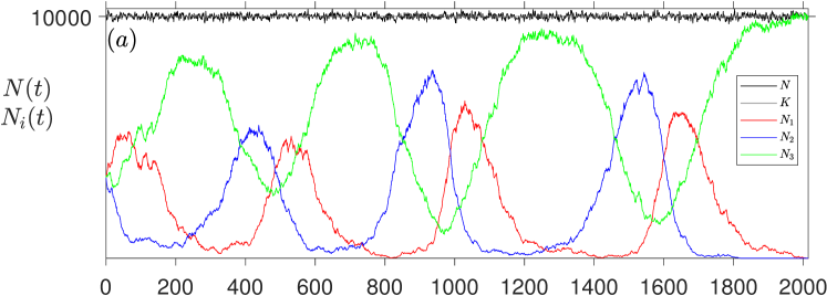
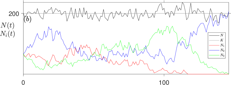
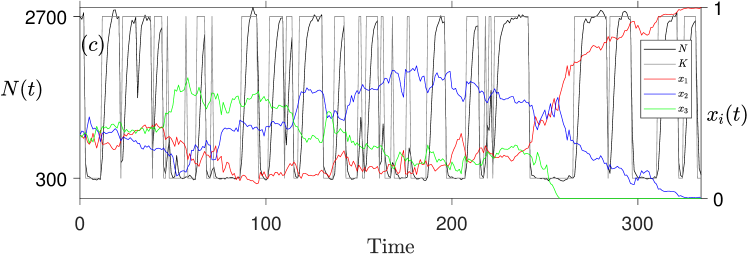
Figure 1: (a,b) Sample paths of $N(t)$ (black), and $N_{i}(t)$ (colored) with constant carrying capacity $K=10^{4}$ in (a) and $K=200$ in (b); solid gray lines show $N(t)=K$. Parameters are $(s,r_{1},r_{2},r_{3})=(1/10,3/5,1/5,1/5)$. $N(t)$ quickly fluctuates about $K$, while $N_{i}$ evolve on a much slower timescale, see text. Fluctuations and extinction properties vary with $sK$, see Sec. 3. (c) Sample paths of $N(t)$ (black), densities $x_{i}(t)=N_{i}(t)/N(t)$ (colored), and typical evolution of the randomly switching $K(t)$ (gray). Parameters are: $(s,r_{1},r_{2},r_{3},\nu,K_{+},K_{-})=(1/20,1/3,1/3,1/3,1/4,2700,300)$. $N(t)$ quickly settles into its (quasi) stationary state while $x_{i}$ vary much more slowly until fixation occurs in a time $\sim\langle K\rangle$, see Sec. 4.2. In all panels: $N_{1}(t),x_{1}(t)$ in red, $N_{2}(t),x_{2}(t)$ in blue, and $N_{3}(t),x_{3}(t)$ in green, $\epsilon=0$. Initially, all species have the same density $1/3$.

Below, we first consider a constant carrying capacity, and then focus on the case where $K$ fluctuates in time. For the fluctuating carrying capacity, we assume that $K(t)$ continuously switches between two values, $K_{+}$ and $K_{-}$. This simply models that available resources continuously and randomly change from being scarce ($K=K_{-}$) to being abundant ($K=K_{+}>K_{-}$). The population size thus varies with $K$ and so do the demographic fluctuations, resulting in IN being coupled to EN. For simplicity, we model the switches of $K(t)$ with a colored dichotomous Markov noise (DMN) [64, 63], or “random telegraph noise”, $\xi(t)\in\{-1,+1\}$ with symmetric switching rate $\nu$:

$$\xi\xrightarrow{\nu}-\xi.$$ (4)

Here, the DMN is always at stationarity: Its average vanishes, $\langle\xi(t)\rangle=0$, and its autocorrelation is $\langle\xi(t)\xi(t^{\prime})\rangle=\exp\left(-2\nu|t-t^{\prime}|\right)$ [64, 63] (here, $\langle\cdot\rangle$ denotes the ensemble average over the DMN). The randomly switching carrying capacity therefore reads [56, 57]

$$K(t)=\frac{1}{2}\left[\left(K_{+}+K_{-}\right)+\xi(t)\left(K_{+}-K_{-}\right)\right],$$ (5)

where $\langle K\rangle=(K_{+}+K_{-})/2$ is its constant average. The constant-$K$ case is recovered by setting $K_{+}=K_{-}$ in (5).

In what is arguably its simplest formulation, see A.1, the RPS dynamics subject to $K(t)$ is here defined in terms of the birth-death process [51, 56]

$$N_{i}\xrightarrow{T_{i}^{+}}N_{i}+1\quad\text{and}\quad N_{i}\xrightarrow{T_{i}^{-}}N_{i}-1,$$ (6)

for the birth ($N_{i}\to N_{i}+1$) and death ($N_{i}\to N_{i}-1$) of an $i$-individual, respectively, with the transition rates

$$T^{+}_{i}=f_{i}N_{i}\quad\text{and}\quad T^{-}_{i}=\frac{N}{K(t)}N_{i},$$ (7)

where the randomly switching carrying capacity is given by (5), while $K(t)=K$ when the carrying capacity is constant. It is worth noting that we consider $0\leq s\leq 1/(1+\epsilon)$, which suffices to ensure $T^{\pm}_{i}\geq 0$. The master equation (ME) associated with the continuous-time birth-death process (6),(7) gives the probability $P(\vec{N},\xi,t)$ to find the population in state $(\vec{N},\xi)=(N_{1},N_{2},N_{3},\xi)$ at time $t$  [82, 83], and reads:

$$\frac{dP(\vec{N},\xi,t)}{dt} = \sum_{i=1}^{3}\left(\mathbb{E}_{i}^{-}-1\right)\left[T^{+}_{i}P(\vec{N},\xi,t)\right]$$

$$+ \sum_{i=1}^{3}\left(\mathbb{E}_{i}^{+}-1\right)\left[T^{-}_{i}P(\vec{N},\xi,t)\right]$$

$$+ \nu\left[P(\vec{N},-\xi,t)-P(\vec{N},\xi,t)\right],$$

where $\mathbb{E}^{\pm}_{i}$ are shift operators, associated with (6), such that $\mathbb{E}^{\pm}_{1}h(N_{1},N_{2},N_{3},t)=h(N_{1}\pm 1,N_{2},N_{3},t)$ etc, for any $h(\vec{N},\xi,t)$, and the last line accounts for the random switching of $K$. In Eq (2), $P(\vec{N},\xi,t)=0$ whenever any $N_{i}<0$. This multidimensional ME can be simulated exactly to fully capture the stochastic RPS dynamics [84]. This is characterized by a first stage in which all species coexist, then two species compete in a second stage, and, after a time that diverges with the system size, the population finally collapses . Here, we focus on the first two stages of the dynamics in which $N(t)$ is characterized by its quasi-stationary distribution ($N$-QSD). In the constant-$K$ case, one drops the last line and sets $K_{+}=K_{-}=K$ in Eq. (2), yielding the underpinning three-dimensional ME for $P(\vec{N},t)$.

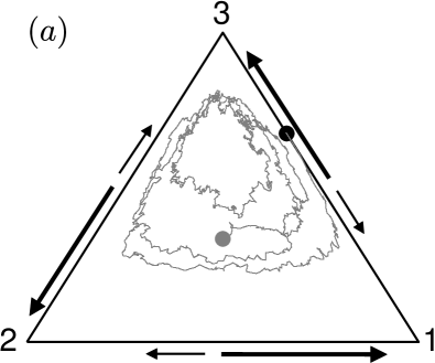
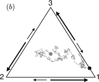
Figure 2: Stochastic orbits in $S_{3}$ of the constant-$K$ BDCLV ($\epsilon=0$) of Fig. 1 (a,b), with $(s,r_{1},r_{2},r_{3})=(1/10,3/5,1/5,1/5)$ and illustration of Stages 1 and 2 of dynamics, see text. Initially all species have the same density $1/3$ (gray dot), and (a) $K=10^{4}$, (b) $K=200$. (a) In Stage 1, when $sK\gg 1$, erratic trajectories approach $\partial S_{3}$ from the outermost orbit (deterministic orbit at a distance $1/K$ from $\partial S_{3}$, see text). (b) When $sK={\cal O}(10)$, in Stage 1, stochastic trajectories reach $\partial S_{3}$ without settling onto the outermost orbit. Stage 2: Once on an edge of $\partial S_{3}$ (black dot), a competition (shown as arrows) takes place between species $i$ and its weak opponent $i+1$, with the former (long arrows) more likely to win than the latter (short arrows), see text.

3 The birth-and-death cyclic Lotka-Volterra model $(\epsilon=0)$ with constant carrying capacity

In order to understand how environmental variability affects the RPS dynamics, it is useful to study first the dynamics of the model defined by (2)-(7) with $\epsilon=0$ when the carrying capacity $K$ is constant. This zero-sum model ($\bar{\Pi}=0,\bar{f}=1$), is referred to as the constant-$K$ birth-and-death cyclic Lotka-Volterra model (BDCLV) and its dynamics is fully described by the underpinning ME. Proceeding as in A.1, the mean-field description of the constant-$K$ BDCLV is obtained by neglecting all fluctuations, yielding

$$\dot{N} = \sum_{i=1}^{3}(T_{i}^{+}-T_{i}^{-})=N\left(1-\frac{N}{K}\right),$$ (9)

$$\dot{x_{i}} = \frac{T_{i}^{+}-T_{i}^{-}}{N}-x_{i}\frac{\dot{N}}{N}=x_{i}[\alpha_{i}x_{i+1}-\alpha_{i-1}x_{i-1}],$$ (10)

where $\alpha_{i}\equiv sr_{i}$, and the dot stands for the time derivative. Clearly, the population size obeys the logistic equation (9), and thus $N(t)\to K$ after a time $t={\cal O}(1)$. The rate equations (REs) for $x_{i}=N_{i}/N$ describe how the population composition changes due to cyclic dominance on a timescale $1/s$. Eqs. (9) and (10) are decoupled and, when $s\ll 1$, there is a timescale separation: $N$ rapidly approaches $K$ while the $x_{i}$’s evolve much slower. When time is rescaled ($t\to st$), the REs (10) coincide with the celebrated replicator equations of the zero-sum RPS game [13, 14, 15, 16, 17]. These REs are characterized by a neutrally stable fixed point $\vec{x}^{*}=\left(r_{2},r_{3},r_{1}\right)$ associated with the coexistence of a fraction $r_{i+1}$ of each species $i$, and three saddle (unstable) fixed points $\left\{\vec{e}_{1}=(1,0,0),\vec{e}_{2}=(0,1,0),\vec{e}_{3}=(0,0,1)\right\}$, $\vec{e}_{i}$ corresponding to a state in which only individuals of species $i$ are present. In addition to conserving $x_{1}+x_{2}+x_{3}=1$, the REs (10) also conserve the quantity $\mathcal{R}=\prod_{i=1}^{3}x_{i}^{r_{i+1}}$. The deterministic trajectories in the phase space $S_{3}$ are therefore neutrally stable orbits surrounding $\vec{x}^{*}$ [14]. The dynamics in a finite population is characterized by noisy oscillations about $\vec{x}^{*}$, see Fig. 1 (a,b), with erratic trajectories performing a random walk between the deterministic orbits until $\partial S_{3}$ is hit and one species goes extinct. This first stage of the dynamics (Stage 1) where the three species coexist is followed by Stage 2 where the two surviving species, say $i$ and $i+1$, compete along the edge $(i,i+1)$ of $S_{3}$ until one them prevails and fixates, see Fig. 2. The population size $N(t)$ is not constant but, after $t={\cal O}(1)$, fluctuates about $K$, with fluctuation intensity that decreases with $K$, see Fig. 1 (a,b). It is worth noting that the population size keeps fluctuating, $N(t)\approx K$, even after Stage 2 when it consists of only the species having fixated in Stage 2, see Footnote 2.

The fact that, after a short transient, $N(t)\approx K$ suggests a relation between the constant-$K$ BDCLV and the cyclic Lotka-Volterra model evolving according to a Moran process in a population of constant size $N=K$ [67, 16, 68, 69], see A.2. In the Moran cyclic Lotka-Volterra model (MCLV), the birth of an $i$-individual and the death of an individual of type $j\neq i$ occurs simultaneously: In the MCLV, an $i$ replaces a $j$ with rate $T_{j\to i}$ and the population size remains constant, see, e.g., [67, 68, 69]. In A.2, the constant-$K$ BDCLV is shown to have the same fixation properties as the MCLV with transition rates $T_{j\to i}=T_{i}^{+}T_{j}^{-}/K$ and $N=K$, see Fig. S1.

It is also useful to compare the constant-$K$ BDCLV with the so-called chemical cyclic Lotka-Volterra model (cCLV), see A.3. In the cCLV, the cyclic competition between the three species is of predator-prey type: An $i$-individual (predator) kills an $(i+1)$-individual (its prey) and immediately replaces it, leaving the population size constant. In A.3, we show that the cCLV admits the same mean-field dynamics as the constant-$K$ BDCLV, see Eq. (S15). However, once a species has gone extinct in the cCLV, there is a predator-prey competition in Stage 2 won by the predator with a probability $1$. Hence, Stage 1 survival and fixation probabilities coincide in the cCLV. Remarkably, it was found that these quantities obey two simple laws, the so-called “law of the weakest” (LOW) when $N$ is large and the “law of stay out” (LOSO) in smaller populations [6, 4, 33], see A.3.1 and Fig. S2.

As detailed in B, the stage 1 dynamics of the constant-$K$ BDCLV is similar to the stage 1 cCLV dynamics in a population of size ${\cal O}(sK)$. The stage 2 dynamics in the constant-$K$ BDCLV and MCLV with $N=K$ are similar, with both surviving species having a non-zero probability to fixate, see B.

In what follows, we exploit the relationships between the BDCLV and the MCLV and cCLV to shed light on its fixation properties when $K$ is constant and randomly switching. In particular, we study the novel survival scenarios that can arise when $N(t)$ fluctuates.

3.1 Survival, absorption and fixation probabilities in the constant-$K$ BDCLV

All three species coexist during Stage 1: In the constant-$K$ BDCLV their fractions erratically oscillate about $\vec{x}^{*}$ until $\partial S_{3}$ is hit, see Figs. 1 (a,b) and 2. Stage 1 ends at this point and is characterized by the probability $\phi_{i,i+1}$ to have reached the edge $(i,i+1)$ (survival of species $i$ and $i+1$) or, equivalently, that species $i-1$ is the first to die out. Once on $\partial S_{3}$, Stage 2 starts and two species, say $i$ and $i+1$, compete along their edge until either $i$, with probability $\phi_{i}$, or $i+1$, with probability $1-\phi_{i}$, get absorbed. Clearly, the stage 2 dynamics is conditioned by the outcome of Stage 1 and the overall fixation probability $\widetilde{\phi_{i}}$ depends on $\phi_{i,j}$ and $\phi_{i}$, see Eq. (17).

Below, we show that $\phi_{i,i+1},\phi_{i}$ and $\widetilde{\phi}_{i}$ are functions of $sK$, see Figs. 3 and 4, and can respectively be inferred from the well-known properties of the cCLV and MCLV, see A. In our discussion, we distinguish three regimes: (i) quasi-neutrality, when $sK\ll 1$ and $K\gg 1$; (ii) weak selection, when $sK={\cal O}(10)$, with $s\ll 1$ and $K\gg 1$; and (iii) strong selection, when $sK\gg 1$, with $s={\cal O}(1)$ and $K\gg 1$. In the examples below, these three regimes are identified as follows: $s\lesssim 1/K$ in regime (i), $1/K\lesssim s\lesssim 100/K$ in regime (ii), and $s\gtrsim 100/K$ in regime (iii), with $K\gg 1$. Furthermore, since the overall fixation probability of each species $\widetilde{\phi_{i}}$ is trivially $1/3$ when $r_{1}=r_{2}=r_{3}=1/3$ [19, 6, 33], we focus on the general case where the $r_{i}$’s are unequal. All figures have been obtained with the initial fraction $1/3$ of each species, i.e. $\vec{x}_{0}\equiv(x_{1}(0),x_{2}(0),x_{3}(0))=\vec{x}_{c}\equiv(1,1,1)/3$, and we consider the following set of parameters: $\vec{r}\equiv(r_{1},r_{2},r_{3})=\vec{r}^{(1)}\equiv(1,5,5)/11$ and $\vec{r}=\vec{r}^{(2)}\equiv(3,1,1)/5$. These choices suffice to reveal most of the generic properties of the system. When we study how $\phi_{i,i+1}$, $\phi_{i}$ and $\widetilde{\phi_{i}}$ depend on $sK$, in Figs. 3 and 4 we consider $K\in\varkappa\equiv\{1000,450,250,90,50\}$ and $s=1$ for $K=1000$, $s\in\{10^{-k/4},k=0\dots 3\}$ for $K=450$, $s\in\{10^{-(2+k)/4},k=0\dots 9\}$ for $K=250$, $s\in\{10^{-k/4},k=0\dots 8\}$ for $K=90$, and $s\in\{10^{-(9+k)/4},k=0\dots 3\}$ for $K=50$. In all figures (except Figs. 1 and 2), simulation results have been sampled over $10^{4}-10^{5}$ realizations.

3.1.1 Stage 1: Survival probabilities in the constant-$K$ BDCLV

The stage 1 dynamics of the constant-$K$ BDCLV and cCLV with $N={\cal O}(sK)$ are similar, see B. The constant-$K$ BDCLV survival probabilities $\phi_{i,j}$ are therefore similar to the survival/fixation probabilities in the cCLV. These obey the LOW when $N$ is large and the LOSO in smaller populations [6, 4, 33], see A.3.1. The LOW and LOSO are here used to determine $\phi_{i,j}$ in regimes (ii) and (iii).

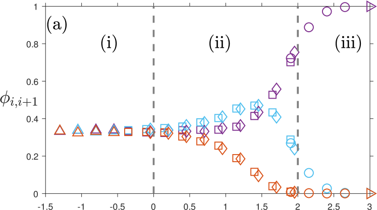
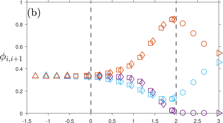
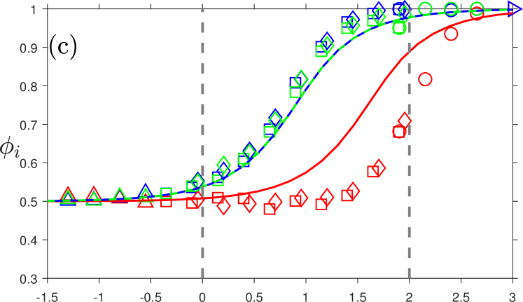
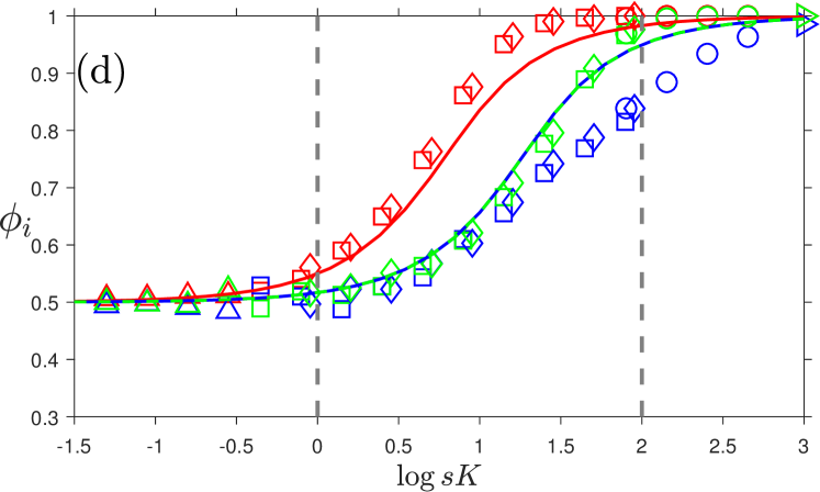
Figure 3: (a,b) Constant-$K$ BDCLV survival probabilities simulation results ($\Diamond$): $\phi_{1,2}$ (purple), $\phi_{2,3}$ (light blue) and $\phi_{3,1}$ (orange) vs. $sK$ for values of $s\in(10^{-3},1)$ and $K\in\varkappa$ in regimes (i)-(iii) separated by dashed lines, see text. Non-monotonicity arises across regimes (ii) and (iii) and can be explained in terms of the LOSO (regime (ii)) and LOW (regime (iii)), see text. (a) $\vec{r}=\vec{r}^{(1)}$; species $1$ and $3$ are the most likely to die out in regime (ii) and (iii), respectively. (b) $\vec{r}=\vec{r}^{(2)}$ ; species $2$ and $1$ are the most likely to die out in regime (ii) and (iii), respectively. (c,d) Constant-$K$ BDCLV absorption probabilities $\phi_{i}$ vs. $sK$: $\phi_{1}$ (red), $\phi_{2}$ (blue) and $\phi_{3}$ (green) vs. $sK$ for $K=(1000,450,250,50,20)$, with (c) $\vec{r}=\vec{r}^{(1)}$ and (d) $\vec{r}=\vec{r}^{(2)}$. The solid line is given by (16) and coincide for species $2$ and $3$. In all panels $K=1000~{}(\rhd),450~{}(\circ),250,~{}(\diamond),90~{}(\square),50~{}(\triangle)$, $\epsilon=0$, $\vec{x}_{0}=\vec{x}_{c}$.

- Regime (i): When $sK\ll 1$, with $K\gg 1$, the system is at quasi-neutrality. The dynamics is driven by demographic fluctuations and all species have the same survival probability $\phi_{i,i+1}\approx 1/3$, see (i) in Fig. 3 (a,b).

- Regime (ii): When $sK={\cal O}(10)$ and $K\gg 1$, the intensity of selection strength is weak ($s\ll 1$) and comparable to that of demographic fluctuations. From the relation with the cCLV, we infer that $\phi_{i,i+1}$ is given by the fixation probability $\phi_{i}^{{\rm cCLV}}|_{sK}$ of species $i$ in the cCLV in a population of size of order $sK$, i.e. $\phi_{i,i+1}\approx\phi_{i}^{{\rm cCLV}}|_{sK}$. In regime (ii), $\phi_{i}^{{\rm cCLV}}|_{sK}$ obeys the LOSO, see A.3.1, and from Eq. (S20) we obtain:

$$\phi_{i-1,i}>\phi_{i,i+1},\phi_{i+1,i-1}\quad\text{if $\quad r_{i}>r_{i\pm 1}$}$$ (11)

$$\phi_{i,i+1}\approx\phi_{i+1,i-1}>\phi_{i-1,i}\quad\text{if $\quad r_{i+1}=r_{i-1}>r_{i}$}.$$

Accordingly, when $r_{i}>r_{i\pm 1}$ species $i-1$ and $i$ are the most likely to survive Stage 1 under weak selection, as confirmed by Fig. 3 (b). When $r_{i+1}=r_{i-1}>r_{i}$ and $sK={\cal O}(10)$, the edges $(i,i+1)$ and $(i+1,i-1)$ are the most likely to be hit, while species $i-1$ is most likely to die out first, see Fig. 3 (a). While the $\phi_{i,j}$’s obey the LOSO, we notice that $\phi_{i,j}\approx 1/3$ when $s\ll 1$.

- Regime (iii): When $sK\gg 1$, with $s={\cal O}(1)$ and $K\gg 1$, the stage 1 dynamics is governed by cyclic dominance. An edge of $S_{3}$ is hit from the system’s outermost orbit as in the cCLV, see B and Fig. 2 (a). From the relation between the constant-$K$ BDCLV and the cCLV, we have $\phi_{i,i+1}\approx\phi_{i}^{{\rm cCLV}}|_{sK}$ which obeys the LOW in regime (iii), and therefore from (S18) we have:

$$\phi_{i,i+1}>\phi_{i+1,i-1},\phi_{i-1,i}\;\text{if $\quad r_{i}<r_{i\pm 1},$ }$$ (12)

$$\phi_{i,i+1}\approx\phi_{i+1,i-1}>\phi_{i-1,i}\;\text{if $\quad r_{i}=r_{i+1}<r_{i-1}$. }$$

When $sK\gtrsim 10^{3}$, the LOW becomes asymptotically a zero-one law: $\phi_{i,i+1}\to 1,\phi_{i-1,i}\to 0$ and $\phi_{i+1,i-1}\to 0$ if $r_{i}<r_{i\pm 1}$, and $\phi_{i,i+1}=\phi_{i+1,i-1}\to 1/2,\phi_{i-1,i+1}\to 0$ if $r_{i}=r_{i+1}<r_{i-1}$, see Eq. (S19). Accordingly, when $sK\gg 1$ and $r_{i}<r_{i\pm 1}$ species $i$ and $i+1$ are most likely to survive and species $i-1$ the most likely to die out in Stage 1, in agreement with Fig. 3 (a).

The relations (11) and (12) explain that $\phi_{i,i+1}$ is a function of $sK$ that can exhibit a non-monotonic behavior. For instance, for $\vec{r}=\vec{r}^{(1)}$ as in Fig. 3 (a), the relations (11) yield $\phi_{1,2}\approx\phi_{2,3}>\phi_{3,1}$ when $sK={\cal O}(10)$, and (12) predict $\phi_{1,2}>\phi_{2,3},\phi_{3,1}$ when $sK\gg 1$, while $\phi_{1,2}\approx\phi_{2,3}\approx\phi_{3,1}\approx 1/3$ when $sK\ll 1$. From these results, it is clear that $\phi_{2,3}$ increases across the regimes (i)-(ii), and then decreases with $sK$ across the regimes (ii)-(iii), whereas $\phi_{1,2}$ and $\phi_{3,1}$ respectively increases and decreases with $sK$ across all regimes.

3.1.2 Stage 2: Absorption probabilities in the constant-$K$ BDCLV

At start of Stage 2, species $i$ competes against $i+1$ (weak opponent), along the edge $(i,i+1)$ where their fitnesses are $f_{i}=1+\alpha_{i}(1-x_{i})$ and $f_{i+1}=1-\alpha_{i}x_{i}$, see (3). Stage 2 ends with the absorption of either $i$ or $i+1$, respectively with probability $\phi_{i}$ and $1-\phi_{i}$.

- At quasi neutrality, species $i$’s selective advantage is negligible since $f_{i}-f_{i+1}=\alpha_{i}\ll 1$. In regime (i), species $i$ and $i+1$ have therefore almost the same absorption probability $\phi_{i}\approx 1/2$.

- Under strong selection, species $i$ has an important selective advantage over species $i+1$: $f_{i}-f_{i+1}={\cal O}(1)$. In regime (iii), species $i$ is almost certain to be absorbed as in Stage 2 of the cCLV dynamics, and therefore $\phi_{i}\approx 1$ as predicted by the LOW, see Appendices A.3 and B.

- Under weak selection, in regime (ii), $\phi_{i}$ is nontrivial and can be obtained from the fixation probability $\phi_{i}|_{K}$ of species $i$ in the MCLV with $N=K$, see Appendices A.2 and C. When the stage 2 dynamics starts with a fraction $\hat{x}_{i}$ of individuals of species $i$, $\phi_{i}|_{K}$ under weak selection is obtained from the backward Fokker-Planck generator

$${\cal G}_{(i,i+1)}|_{K}=\frac{x_{i}(1-x_{i})}{K}\left[K\alpha_{i}\frac{d}{dx_{i}}+\frac{d^{2}}{dx_{i}^{2}}\right],$$ (13)

by solving ${\cal G}_{(i,i+1)}|_{K}(\hat{x}_{i})\phi_{i}|_{K}(\hat{x}_{i})=0$ with $\phi_{i}|_{K}(1)=1-\phi_{i}|_{K}(0)=1$, see Eq. (S24), yielding

$$\phi_{i}\simeq\phi_{i}(\hat{x_{i}})|_{K}=\frac{1-e^{-\alpha_{i}K\hat{x_{i}}}}{1-e^{-\alpha_{i}K}}.$$ (14)

A difficulty arises from $\hat{x_{i}}$ being a random variable depending on the outcome of Stage 1: $\hat{x_{i}}$ is distributed according to the probability density $P_{(i,i+1)}(\hat{x_{i}})$. The absorption probability is thus obtained by averaging (14) over $P_{(i,i+1)}$:

$$\phi_{i}\simeq\phi_{i}|_{K}=\int_{0}^{1}P_{(i,i+1)}(\hat{x_{i}})~{}\phi_{i}(\hat{x_{i}})|_{K}~{}d\hat{x_{i}}.$$ (15)

In practice, $P_{(i,i+1)}(\hat{x_{i}})$ is obtained from stochastic simulations, see D. Analytical progress can be made by noticing that in regime (ii) where $s\ll 1$ and $sK\lesssim 10$, each pair $i,i+1$ has approximately the same survival probability at the end of Stage 1 ($\phi_{i,i+1}\approx 1/3$, see Fig. 3 (a,b)), and the initial distribution along $(i,i+1)$ can be assumed to be uniform, i.e. $P_{i,i+1}(\hat{x}_{i})\approx 1$, see Fig. S3. Substituting in Eq. (15), we obtain the approximation ($s\ll 1,sK\lesssim 10$):

$$\phi_{i}\simeq\phi_{i}|_{K}\approx\frac{e^{-\alpha_{i}K}+\alpha_{i}K-1}{\alpha_{i}K(1-e^{-\alpha_{i}K})},$$ (16)

which is an S-shaped function of $\alpha_{i}K$ that correctly predicts the behaviors $\phi_{i}\to 1/2$ when $\alpha_{i}K\ll 1$ (regime (i)) and $\phi_{i}\to 1$ when $\alpha_{i}K\gg 1$ (regime (iii)), see Fig. 3 (c,d). Comparison with simulation results of Fig. 3 (c,d) confirm that $\phi_{i}$ is sigmoid function of $sK$ and Eq. (16) provides a good approximation of $\phi_{i}$ when the assumption $P_{(i,i+1)}\approx 1$ holds, see Fig. S3.

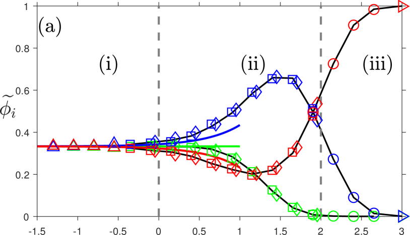
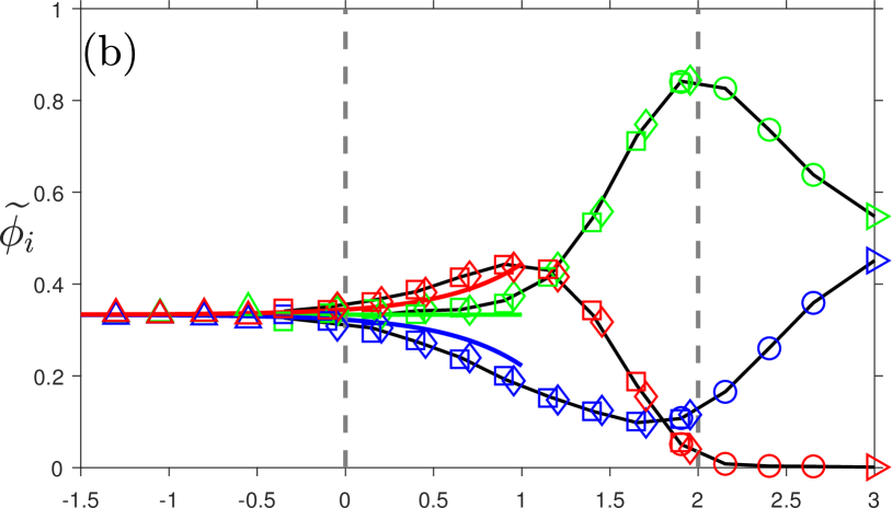
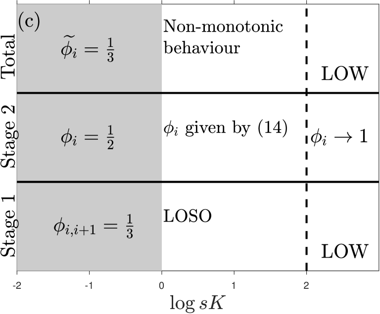
Figure 4: (a,b) Total fixation probabilities $\widetilde{\phi}_{1}$ (red), $\widetilde{\phi}_{2}$ (blue), $\widetilde{\phi}_{3}$ (green) vs. $sK$ for values of $s\in(10^{-3},1)$ and $K\in\varkappa$ with symbols as in Fig. 3, see text. Regimes (i)-(iii), from left to right, are indicatively separated by dashed gray lines. (a) $\vec{r}=\vec{r}^{(1)}$; (b) $\vec{r}=\vec{r}^{(2)}$. The solid black lines show the predictions of (17) using (15), with $\phi_{i,i+1}$ and $P_{(i,i+1)}$ inferred from simulations. Predictions from (19) are shown as solid colored line. $\widetilde{\phi}_{i}$ can display a non-monotonic dependence on $sK$ across regimes (ii)-(iii), see text. (c) Chart summarizing the outcome of Stage 1, Stage 2 and the overall fixation probability $\widetilde{\phi}_{i}$ as function of $sK$ in regimes (i)-(iii), from left to right. In all panels: $\vec{x}_{0}=\vec{x}_{c}$ and $\epsilon=0$.

3.1.3 Total fixation probabilities in the constant-K BDCLV

Species $i$’s total fixation probability $\widetilde{\phi}_{i}$ consists of two contributions: $\phi_{i,i+1}\phi_{i}$ and $\phi_{i-1,i}(1-\phi_{i-1})$. The first one counts the probability for $i$ to fixate after hitting the edge $(i,i+1)$, with a probability $\phi_{i,i+1}$, and prevailing against $i+1$ (weak opponent) with a probability $\phi_{i}$. We also need to consider that, after reaching the edge $(i-1,i)$ with a probability $\phi_{i-1,i}$, species $i$ has a probability $1-\phi_{i-1}$ to win against $i-1$ (strong opponent), which yields $\phi_{i-1,i}(1-\phi_{i-1})$. With these two contributions, we obtain

$$\widetilde{\phi}_{i}=\phi_{i,i+1}\phi_{i}+\phi_{i-1,i}(1-\phi_{i-1}),$$ (17)

which is also a function of $sK$, see Fig. 4 (a,b). Of particular interest is the situation where the selection intensity is weak, $s\ll 1$, in which case (17) can be simplified by noting $\phi_{i,i+1}\approx\phi_{i-1,i}\simeq 1/3$ and using the result $\phi_{i}\simeq\phi_{i}|_{K}$, given by (16), for the absorption probability in the MCLV with $N=K$, see A.2, yielding

$$\widetilde{\phi}_{i}\simeq\frac{1}{3}\left(1+\phi_{i}-\phi_{i-1}\right)\approx\frac{1}{3}\left(1+\phi_{i}|_{K}-\phi_{i-1}|_{K}\right).$$ (18)

Using the properties of the survival and absorption probabilities $\phi_{i,j}$ and $\phi_{j}$ discussed above, we can infer those of $\widetilde{\phi}_{i}$ in the regimes (i)-(iii):
- Regime (i): At quasi-neutrality, all species have the same fixation probability to first order: $\widetilde{\phi}_{i}=1/3+{\cal O}(sK)$. An estimate of the subleading correction is obtained by noticing $\phi_{i}|_{K}\simeq\frac{1}{2}\left(1+\alpha_{i}K/6\right)$ when $\alpha_{i}K\ll 1$. This, together with Eq. (18), gives

$$\widetilde{\phi}_{i}\simeq\frac{1}{3}\left(1+\frac{sK}{12}(r_{i}-r_{i-1})\right).$$ (19)

This result allows us to understand which are the species (slightly) favored by selection: When $r_{1}<r_{2},r_{3}$, Eq. (19) predicts that $\widetilde{\phi}_{1}$ is less than $1/3$ and decreases with $sK$, while $\widetilde{\phi}_{2}>1/3$ and increases with $sK$, and $\widetilde{\phi}_{3}=1/3+{\cal O}(s^{2})$. These predictions agree with the simulation results of Fig. 4 (a) in regime (i).
- Regime (iii): Under strong selection, the total fixation probability obeys the LOW, as in the cCLV (see B). The species overall fixation probabilities are therefore ordered as follows, see Eqs. (S18, S19):

$$\widetilde{\phi}_{i}>\widetilde{\phi}_{i+1},\widetilde{\phi}_{i-1}\quad\text{if \quad$r_{i}<r_{i\pm 1},\;\;\;$ and \;\;\;}$$

$$\widetilde{\phi}_{i}\approx\widetilde{\phi}_{i+1}>\widetilde{\phi}_{i-1}\quad\text{if}\quad r_{i}=r_{i+1}<r_{i-1},$$ (20)

with $\widetilde{\phi}_{i}\approx\phi_{i,i+1}\overset{sK\gg 1}{\longrightarrow}1$, $1/2$ or $0$. These predictions agree with the simulations results of Fig. 4 (a,b).
- Regime (ii): Under weak selection, $\widetilde{\phi}_{i}$ can vary non-monotonically with $sK$, see Fig. 4 (a,b). This behavior can be understood by noticing that near the boundary of regimes (i)-(ii), we have $\phi_{i}\approx 1/3$ that increases with $sK$ if $r_{i}>r_{i-1}$ and decreases when $r_{i}<r_{i-1}$, see Eq. (19) and Fig. 4 (a,b). As $sK$ approaches the boundary of regimes (ii)-(iii), the dynamics is increasingly governed by the LOW with $\widetilde{\phi}_{i}\approx\phi_{i,i+1}\overset{sK\gg 1}{\longrightarrow}1$, $1/2$ or $0$. This can lead to a non-monotonic dependence on $sK$: For instance, if $r_{1}<r_{2},r_{3}$, $\widetilde{\phi}_{1}$ decreases and $\widetilde{\phi}_{2}$ increases about the value $1/3$ near the (i)-(ii) boundary, and then respectively increases and decreases as $sK$ approaches the boundary (ii)-(iii), and through regime (iii) where $\widetilde{\phi}_{1}\to 1$ while $\widetilde{\phi}_{2}\to 0$, see Fig. 4 (a).

The main features of the survival, absorption and overall fixation probabilities in the constant-$K$ BDCLV are summarized in the chart of Fig. 4 (c).

3.2 Mean fixation time in the constant-$K$ BDCLV

The overall mean fixation time $T_{F}$ is the average time after which one of the species takes over the entire population. This quantity consists of one contribution arising from Stage 1, referred to as the mean extinction time $T_{1}$, and the mean absorption time $T_{2}$ arising from Stage 2. In E.1, we study $T_{1}$ and $T_{2}$ in the regimes (i)-(iii) and show that, when $\vec{x}_{0}=\vec{x}_{c}$, the overall mean fixation time $T_{F}=T_{1}+T_{2}={\cal O}(K)$, see Fig. S4(c). Since $N(t)\simeq K$ after a short transient, this means that species coexistence is lost after a mean time scaling linearly with the population size. We also show that $T_{1}$ and $T_{2}$ are both of order ${\cal O}(K)$ in regimes (i)-(ii) and $T_{1}\gg T_{2}$ in the regime (iii), see Figs. S4 (a,b) and 1.

4 CLV with randomly switching carrying capacity

In many biological applications, the population is subject to sudden and extreme environmental changes dramatically affecting its size [60, 59, 52, 53, 54]. The variation of $N(t)$ leads to a coupling between demographic fluctuations which greatly influence the population’s evolution  [56, 57, 52, 53, 54].

Here, we study the coupled effect of demographic and environmental fluctuations on the BDCLV fixation properties by considering the randomly-switching carrying capacity (5), modeled in terms of the stationary DMN (4), that can also be written as

$$K(t)=\langle K\rangle(1+\gamma\xi(t)),\quad\text{with $\gamma\equiv\frac{K_{+}-K_{-}}{2\langle K\rangle}$}$$

where $0<\gamma<1$ is a parameter measuring the intensity of the environmental variability. In fact, the variance of $K(t)$ is ${\rm var}(K(t))=(\gamma\langle K\rangle)^{2}$, and we can write $K_{\pm}=(1\pm\gamma)\langle K\rangle$. In order to study the influence of environmental variability on the population dynamics, we consider $\gamma={\cal O}(1)$ and $\langle K\rangle\gg 1$. This ensures that the population is subject to significant environmental variability (${\rm var}(K)\gg 1$), and its typical size is large enough to avoid that demographic fluctuations (internal noise, IN) alone are the main source of randomness. In all our simulations, the initial value of $K(t)$ is either $K_{+}$ or $K_{-}$ with probability $1/2$.

From the ME (2), proceeding as in A.1, the population composition is found to still evolve according to the REs (10) when all demographic fluctuations are neglected. However, now the random switching of $K(t)$ drives the stochastic evolution of the population size which, when IN is ignored, obeys $\dot{N}=N(1-N/K_{\pm})$ if $\xi=\pm 1$, see Eq. (S8). This can be rewritten as

$$\dot{N} = N\left(1-\frac{N}{{\cal K}}\{1-\gamma\xi(t)\}\right)\,,$$ (21)

where

$${\cal K}\equiv(1-\gamma^{2})\langle K\rangle=\frac{2K_{+}K_{-}}{K_{+}+K_{-}}$$

is the harmonic mean of $K_{\pm}$ and $\xi$ is the multiplicative dichotomous noise (4). The DMN intensity being $N^{2}\gamma/{\cal K}$, the environmental fluctuations increase with $\gamma$ together with ${\rm var}(K)=(\gamma\langle K\rangle)^{2}$. Eq. (21) defines a piecewise-deterministic Markov process (PDMP) [66]. When $\nu\to\infty$, the DMN self averages, with $\xi\to\langle\xi\rangle=0$ in (21) which reduces to the logistic equation (9) with a renormalized carrying capacity $K\to{\cal K}$ [56, 57]. Again, a timescale separation arises when $s\ll 1$, with $N$ evolving faster than $x_{i}$’s: $N$ settles in its $N$-QSD in a time $t={\cal O}(1)$, while the $x_{i}$’s change on a timescale $t={\cal O}(1/s)$, see Fig. 1 (c).

The PDMP defined by Eq. (21) [63, 64, 43, 56, 57] is characterized by the following stationary marginal probability density function (pdf) [56]:

$$p_{\nu}^{*}(N)=\frac{\mathcal{Z}}{N^{2}}\left[\frac{(K_{+}-N)(N-K_{-})}{N^{2}}\right]^{\nu-1},$$ (22)

where $\mathcal{Z}$ is the normalization constant. The PDMP pdf $p_{\nu}^{*}$ gives the long-time probability density of $N$ on the support $N\in[K_{-},K_{+}]$ regardless of the environmental state $\xi$ [63, 64]. When $\gamma={\cal O}(1)$ and $\langle K\rangle\gg 1$, $p_{\nu}^{*}$ is a good approximation of the $N$-QSD even if it ignores the effect of the IN, see Fig. 5.

Figure 5: $N$-QSD and $p^{*}_{\nu}(N)$ for (a) $\nu=0.01$, (b) $\nu=0.1$, (c) $\nu=2$, (d) $\nu=10$. Parameters are $(s,K_{+},K_{-})=(0.02,450,50)$. Solid lines are histograms from stochastic simulations and colored dashed lines are PDMP predictions from (22), see text. Black dashed lines indicate $N=K_{\pm}$ in (a) and (b), $N=N^{*}$ in (c), and $N={\cal K}$ in (d), see text.

In fact, the comparison of $p_{\nu}^{*}$ and $N$-QSD shown in Fig. 5 reveals that $p_{\nu}^{*}$ correctly captures the main features of the $N$-QSD, such as the location of the peak(s) and its right-tailed skewness, whereas it fails to capture the width about the peak(s) . However, for our purposes here the PDMP approximation is sufficient to characterize the system’s fixation properties [56, 57]. It is noteworthy that $p_{\nu}^{*}$ and the $N$-QSD are bimodal if $\nu<1$, with peaks at $N\simeq K_{\pm}$, see Fig. 5 (a,b). When $\nu>1$, $p^{*}_{\nu}$ and $N$-QSD are unimodal and $N$ fluctuates about the maximum of $p^{*}_{\nu}$ given by $N^{*}=\langle K\rangle(1+\nu)\left(1-\sqrt{1-4\nu(1-\gamma^{2})/(1+\nu)^{2}}\right)/2$. The value of $N^{*}$ increases with $\nu$ at $\gamma$ fixed, see Fig. 5 (c,d), and decreases with $\gamma$ (environmental variability) at $\nu$ fixed. When $\nu\to\infty$, we have $N^{*}\to{\cal K}$ and $p^{*}_{\nu}$ is sharply peaked about ${\cal K}$, as expected from the self-averaging of $\xi(t)$ when $\nu\gg 1$, see Fig. 5 (d). In this case, we recover the constant-$K$ BDCLV dynamics with $K\to{\cal K}$.

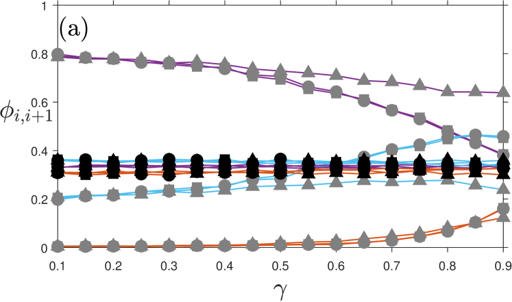
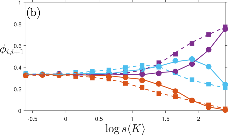
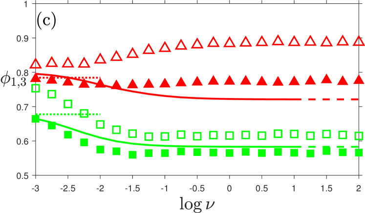
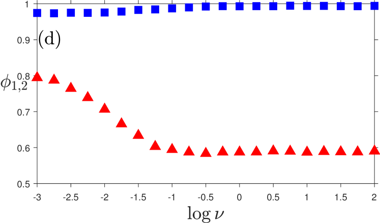
Figure 6: (a) Stage 1 survival probability $\phi_{i,i+1}$ vs. $\gamma$ for $\langle K\rangle=250$ kept fixed ($K_{+}\in[275,475]$ and $K_{-}\in[25,225]$). and $s=0.01$ (black), $s=0.4$ (gray). Simulation results for $\nu=10$ (circles), $\nu=1.2$ (squares) and $\nu=0.001$ (triangles). (b) $\phi_{i,i+1}$ vs. $s\langle K\rangle$ for $\langle K\rangle=250,\gamma=0.8$ and $s\in\{10^{-k/4},k=0,\dots,12\}$ kept fixed, with $\nu=2$ (circles) and $\nu=0.001$ (squares); lines are $\phi_{i,j}|_{(1-\gamma^{2})\langle K\rangle}$ (solid) and $\frac{1}{2}(\phi_{i,j}|_{(1+\gamma)\langle K\rangle}+\phi_{i,j}|_{(1-\gamma)\langle K\rangle})$ (dashed) are from the constant-$\langle K\rangle$ BDCLV. In panels (a,b) $\vec{r}=\vec{r}^{(1)}$, $\phi_{1,2}$ in purple, $\phi_{2,3}$ in light blue, $\phi_{3,1}$ in orange. (c) Stage 2 absorption probabilities $\phi_{1}$ (red triangles) and $\phi_{3}$ (green squares) vs. $\nu$ for $\langle K\rangle=250$ and $\gamma=0.8$ kept fixed and $\vec{r}=\vec{r}^{(2)}$. Symbols are from simulations with $s=0.1$ (open) and $s=10^{-5/4}\approx 0.056$ (filled). Lines are from (27) (solid), (26) (dashed), (25) (dotted), and assume $P_{i,i+1}\approx 1$; they capture reasonably well the $\nu$-dependence of $\phi_{1}$ and $\phi_{3}$ when $s\langle K\rangle\lesssim 10$, see text. (d) Same as in panel (c) for $\phi_{1}$ (red triangles) and $\phi_{2}$ (blue squares) vs. $\nu$ with $s=10^{-1/4}$ and $\vec{r}=\vec{r}^{(1)}$. In all panels $\vec{x}_{0}=\vec{x}_{c}$, $\epsilon=0$.

4.1 Survival, absorption and fixation probabilities in the switching-$K$ BDCLV

As in the constant-$K$ BDCLV, the total fixation probability $\widetilde{\phi}_{i}$ depends on the stage 1 survival and stage 2 absorption probabilities. Here, we analyze the effect of the environmental randomness on these quantities, by distinguishing again the regimes of (i) quasi-neutrality, where $s\ll 1$ and $s\langle K\rangle\ll 1$; (ii) weak selection, where $s\ll 1$ and $s\langle K\rangle={\cal O}(10)$; and (iii) strong selection, where $s={\cal O}(1)$ and $sK\gg 1$.

4.1.1 Stage 1: Survival probabilities in the switching-$K$ BDCLV

To analyze the survival probability $\phi_{i,i+1}$ in the switching-$K$ BDCLV, it is convenient to consider this quantity in the limits $\nu\to\infty$ and $\nu\to 0$, where $\phi_{i,i+1}$ can be expressed in terms of $\phi_{i,i+1}|_{K}$, the survival probability in the constant-$K$ BDCLV studied in Sec. 3.1.1.

When $\nu\to\infty$, many switches occur in Stage 1 and the DMN self averages, $\xi\to\langle\xi\rangle=0$ [56, 57]. The population thus rapidly settles in its $N$-QSD that is delta-distributed at $N=(1-\gamma^{2})\langle K\rangle$ when $\langle K\rangle\gg 1$. Hence, the stage 1 dynamics under fast switching is similar to the cCLV dynamics in a population of size $(1-\gamma^{2})s\langle K\rangle$, see B. This yields $\phi_{i,i+1}\overset{\nu\to\infty}{=}\phi_{i,i+1}|_{(1-\gamma^{2})\langle K\rangle}$.

When $\nu\to 0$, there are no switches in Stage 1, and the extinction of the first species is equally likely to occur in each environmental state $\xi=\pm 1$ (with $K=(1\pm\gamma)\langle K\rangle$). This gives $\phi_{i,i+1}\overset{\nu\to 0}{=}\left(\phi_{i,i+1}|_{(1+\gamma)\langle K\rangle}+\phi_{i,i+1}|_{(1-\gamma)\langle K\rangle}\right)/2$.

The case of intermediate $\nu$ can be inferred from the above by noting that the average number of switches occurring in Stage 1 is ${\cal O}(\nu\langle K\rangle)$, see Fig. S6 (a). As the population experiences a large number of switches in Stage 1 when $\nu={\cal O}(1)$ and $\langle K\rangle\gg 1$, the DMN effectively self-averages, $\xi(t)\simeq\langle\xi\rangle=0$, and therefore

$$\phi_{i,i+1}\overset{\nu={\cal O}(1)}{\approx}\phi_{i,i+1}|_{(1-\gamma^{2})\langle K\rangle}.$$ (23)

When $\nu\ll 1/\langle K\rangle$, there are very few or no switches after a time of order ${\cal O}(\langle K\rangle)$ prior to extinction the first species, and therefore

$$\phi_{i,i+1}\overset{\nu\ll 1/\langle K\rangle}{\approx}\frac{1}{2}\left(\phi_{i,i+1}|_{(1+\gamma)\langle K\rangle}+\phi_{i,i+1}|_{(1-\gamma)\langle K\rangle}\right).$$ (24)

Eq. (23) implies that for any $\nu={\cal O}(1)$, the survival probability of species $i,i+1$, i.e the probability that species $i-1$ dies out first, is given by the survival probability in the constant-$K$ BDCLV with $K=\langle K\rangle$ (same average carrying capacity) and a rescaled selection intensity $(1-\gamma^{2})s$. The effect of random switching is therefore to effectively reduce the selection intensity by a factor $1-\gamma^{2}=1-({\rm var}(K(t))/\langle K\rangle^{2})$ proportional to the variance of the carrying capacity. The $s\langle K\rangle$-dependence of $\phi_{i,i+1}$ can thus readily be obtained from Fig. 3 (a,b) by rescaling $s\to(1-\gamma^{2})s$ as shown in Fig. 6 (a,b). Hence, when there is enough environmental variability ($\gamma$ large enough) the survival scenarios differ from those of the constant-$K$ BDCLV and depend on the switching rate:
- When $\nu\gg 1/\langle K\rangle$, switching reduces the selection by a factor $1-\gamma^{2}$, see Fig. 6 (b). Hence, there is a critical $\gamma^{*}$, estimated as $\gamma^{*}\approx(1-50/s\langle K\rangle)^{1/2}$, such that $\phi_{i,i+1}$ obeys the LOSO when $\gamma>\gamma^{*}$ and $s\langle K\rangle\gg 1$, while the LOW still applies when $\gamma<\gamma^{*}$. Therefore, when $\gamma>\gamma^{*}$, all species have a finite chance to survive Stage 1, with probabilities ordered according to the LOSO, ($\phi_{1,2}\approx\phi_{2,3}>\phi_{3,1}$ with $\gamma^{*}\approx 0.7$, in Fig. 6 (a)). Fig. 6 (a), also shows that the exact value $\nu$ has little influence on $\phi_{i,i+1}$ provided that $\nu\langle K\rangle\gg 1$ (circles and squares almost coincide).
- When $\nu\ll 1/\langle K\rangle$, we have $\phi_{i,i+1}\approx(\phi_{i,i+1}|_{K_{+}}+\phi_{i,i+1}|_{K_{-}})/2$. Hence, if $s\langle K\rangle\gg 1$ and $\gamma>\hat{\gamma}$, where $\hat{\gamma}\approx 1-50/s\langle K\rangle$, $\phi_{i,i+1}|_{K_{+}}$ follows the LOW whereas $\phi_{i,i+1}|_{K_{-}}$ obeys the LOSO, and the $\phi_{i,i+1}$’s therefore interpolate between LOW and LOSO values: For $\gamma>\hat{\gamma}$, the survival probabilities under strong selection and slow switching deviate markedly from the purely LOW values of $\phi_{i,i+1}|_{\langle K\rangle}$ which asymptotically approach $0$, $1$ or $1/2$ (see triangles in Fig. 6 (a) where $\hat{\gamma}\approx 0.5$).

When $s\ll 1$ and $s\langle K\rangle={\cal O}(10)$ in regime (ii), changing $\gamma$ has little effect on the survival probabilities: the survival probabilities $\phi_{i,i+1}\approx 1/3$, and remain ordered according to the LOSO (see black symbols in Fig. 6 (a)).

These results show that environmental variability leads to new survival scenarios in the BDCLV under strong selection: When there is enough variability, all species have a finite probability to survive even when $s\langle K\rangle\gg 1$. The departure from the pure LOW survival scenario is most marked in the generic case of a finite switching rate ($\nu\gg 1/\langle K\rangle$). With respect to the constant-$K$ BDCLV, the general effect of random switching in Stage 1 is therefore to “level the field” by hindering the onset of the zero-one LOW. Since BDCLV survival probability $\phi_{i,i+1}$ coincides with the fixation probability of species $i$ in the cCLV, see B, it is noteworthy that these results also show that random switching can lead to new survival/fixation scenarios in the cCLV when the variance of the carrying capacity is sufficiently high.

4.1.2 Stage 2: Absorption probabilities in the switching-$K$ BDCLV

Stage 2 consists of the competition between types $i$ and $i+1$ along the edge $(i,i+1)$ of $S_{3}$. This starts with an initial fraction $\hat{x}_{i}$ of $i$ individuals and ends up with the absorption of one of the species with probabilities $\phi_{i}$ (for species $i$) and $1-\phi_{i}$ (for $i+1$). Again $\hat{x}_{i}$ is randomly distributed according to a probability density $P_{(i,i+1)}$ resulting from Stage 1, see D. Since $\phi_{i}\approx 1/2$ at quasi-neutrality and $\phi_{i}\approx 1$ under strong selection, see Fig. 6 (c,d), Stage 2 dynamics is nontrivial in regime (ii). To analyze the stage 2 dynamics under weak selection $s\ll 1$ and $\langle K\rangle\gg 1$, it is again useful to consider the limits $\nu\to 0$ and $\nu\to\infty$:

- When $\nu\to 0$, there are no switches in Stage 2 and absorption is equally likely to occur in the static environment $K=K_{-}$ or $K=K_{+}$. Hence, if the fraction $\hat{x}_{i}$ is known, we have $\phi_{i}(\hat{x}_{i})\overset{\mathrm{\nu\to 0}}{=}\phi_{i}^{(0)}(\hat{x}_{i})=\frac{1}{2}\left(\phi_{i}(\hat{x}_{i})|_{K_{-}}+\phi_{i}(\hat{x}_{i})|_{K_{+}}\right)$, where $\phi_{i}(\hat{x_{i}})|_{K}=(1-e^{-\alpha_{i}K\hat{x_{i}}})/(1-e^{-\alpha_{i}K})$, see (14). Since $\hat{x}_{i}$ is randomly distributed, one needs to integrate over $P_{(i,i+1)}$: $\phi_{i}\overset{\mathrm{\nu\to 0}}{\equiv}\phi_{i}^{(0)}=\int_{0}^{1}\phi_{i}^{(0)}(\hat{x}_{i})P_{(i,i+1)}(\hat{x}_{i})~{}d\hat{x}_{i}$. In general, $P_{(i,i+1)}$ is obtained from stochastic simulations and has been found to be mostly independent of $\nu$, see Fig. S3 (c,d). When $s\ll 1$ with $s\langle K\rangle\lesssim 10$, we can again assume $P_{(i,i+1)}\approx 1$ (uniform distribution), which allows us to obtain

$$\phi_{i}\overset{\mathrm{\nu\to 0}}{=}\phi_{i}^{(0)}\simeq\frac{1}{2}~{}\left(\phi_{i}|_{K_{-}}+\phi_{i}|_{K_{+}}\right),\quad\text{where}$$ (25)

$\phi_{i}|_{K}\equiv(e^{-\alpha_{i}K}+\alpha_{i}K-1)/(\alpha_{i}K(1-e^{-\alpha_{i}K}))$, see (16).

- When $\nu\to\infty$, the DMN self averages ($\xi\to\langle\xi\rangle=0$) [56, 57], and the absorption occurs subject to the effective $K(t)={\cal K}$, see Eq. (21). Hence, when $\hat{x}_{i}$ is known, $\phi_{i}(\hat{x}_{i})\overset{\mathrm{\nu\to\infty}}{=}\phi_{i}^{(\infty)}(\hat{x}_{i})=\phi_{i}(\hat{x}_{i})|_{{\cal K}}$, whose integration over $P_{(i,i+1)}$ gives the absorption probability: $\phi_{i}\overset{\mathrm{\nu\to\infty}}{\equiv}\phi_{i}^{(\infty)}=\int_{0}^{1}~{}\phi_{i}^{(\infty)}(\hat{x}_{i})~{}P_{(i,i+1)}(\hat{x}_{i})~{}d\hat{x}_{i}$. When $s\ll 1$ with $s\langle K\rangle\lesssim 10$, and $P_{(i,i+1)}\approx 1$, we have

$$\phi_{i}\overset{\mathrm{\nu\to\infty}}{=}\phi_{i}^{(\infty)}\simeq\phi_{i}|_{{\cal K}}=\frac{e^{-\alpha_{i}{\cal K}}+\alpha_{i}{\cal K}-1}{\alpha_{i}{\cal K}(1-e^{-\alpha_{i}{\cal K}})}.$$ (26)

- When the switching rate $\nu$ is finite and $s\ll 1$, with $s\langle K\rangle={\cal O}(10)$, the probability $\phi_{i}$ can be computed as in Ref. [56] by exploiting the time scale separation between $N$ and $x_{i}$, and by approximating the $N$-QSD by the PDMP marginal stationary probability density (22). In this framework, $\phi_{i}$ can be computed by averaging $\phi_{i}(\hat{x}_{i})|_{N}=(1-e^{-\alpha_{i}N\hat{x_{i}}})/(1-e^{-\alpha_{i}N})$ over the rescaled PDMP probability (22) [56, 57]:

$$\phi_{i}(\hat{x}_{i})\simeq\phi_{i}^{(\nu)}(\hat{x}_{i})=\int_{K_{-}}^{K_{+}}\phi_{i}(\hat{x}_{i})|_{N}~{}p^{*}_{\nu/\alpha_{i}}(N)~{}dN,$$

where $p^{*}_{\nu/\alpha_{i}}$ is given by (22) with a rescaled switching rate $\nu\to\nu/\alpha_{i}$ due to an average number ${\cal O}(\nu/\alpha_{i})$ of switches occurring in Stage 2, see [57] and Sec. E.3. As above, the absorption probability is obtained by formally integrating over $P_{(i,i+1)}$, i.e. $\phi_{i}\simeq\phi_{i}^{(\nu)}\equiv\int_{0}^{1}\phi_{i}^{(\nu)}(\hat{x}_{i})~{}P_{(i,i+1)}({x}_{i})~{}d\hat{x}_{i}$. Under weak selection, we can approximate $P_{(i,i+1)}\approx 1$, see Sec. S4, and, using (15) and (16), we obtain

$$\phi_{i}\simeq\phi_{i}^{(\nu)}\approx\int_{K_{-}}^{K_{+}}\left\{\frac{e^{-N\alpha_{i}}+\alpha_{i}N-1}{\alpha_{i}N\left(1-e^{-\alpha_{i}N}\right)}\right\}~{}p^{*}_{\nu/\alpha_{i}}(N)~{}dN.$$ (27)

The uniform approximation of $P_{(i,i+1)}\approx 1$ is legitimate when $s\langle K\rangle={\cal O}(10)$, and has broader range applicability than in the constant-$K$ case, see Sec. S4 and Fig. S3. Hence, Eq. (27), along with (25) and (26), captures the $\nu$-dependence of $\phi_{i}$ over a broad range of values $\nu$ when $s\ll 1$. In fact, simulation results of Fig. 6 (c,d) show that the $\phi_{i}$’s generally have a non-trivial $\nu$-dependence. When $s\ll 1$ and $s\langle K\rangle={\cal O}(10)$, this is satisfactorily captured by (25)-(27), with $\phi_{i}^{(\nu)}\approx\phi_{i}^{(0)}$ when $\nu\ll 1$, and $\phi_{i}^{(\nu)}\approx\phi_{i}^{(\infty)}$ when $\nu\gg 1$, see Fig. 6 (c, filled symbols). Clearly, the assumption $P_{(i,j)}\approx 1$ and the timescale separation break down when $s={\cal O}(1)$ [57], and the approximations (25)-(27) are then no longer valid.

4.1.3 Overall fixation probabilities in the switching-$K$ BDCLV

The overall fixation probability $\widetilde{\phi}_{i}$ is obtained from the survival and absorption probabilities according to $\widetilde{\phi}_{i}=\phi_{i,i+1}\phi_{i}+\phi_{i-1,i}(1-\phi_{i-1})$, see Eq. (17).

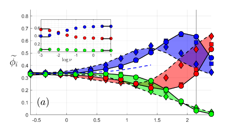
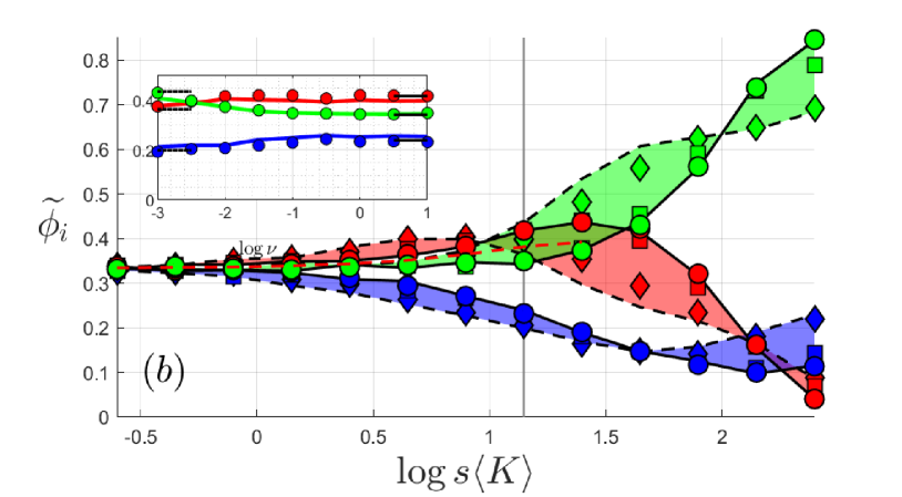
Figure 7: Total fixation probabilities $\widetilde{\phi}_{i}$ vs. $s\langle K\rangle$ for values of $s\in(10^{-3},1)$ and with $\langle K\rangle=250$ and $\gamma=0.8$ kept fixed, see text. (a) $\vec{r}=\vec{r}^{(1)}$; (b) $\vec{r}=\vec{r}^{(2)}$. Shaded areas and symbols are from stochastic simulations with $\nu=10$ ($\circ$), $\nu=0.1$ ($\square$), $\nu=10^{-5/2}$ ($\diamond$). Solid and dashed black lines show respectively $\widetilde{\phi}_{i}|_{{\cal K}}$ and $(\widetilde{\phi}_{i}|_{K_{-}}+\widetilde{\phi}_{i}|_{K_{+}})/2$ in both panels and insets, see text. Vertical light gray lines indicate $\widetilde{\phi}_{i}$ for $s=10^{-1/4}$ (a) and $s=10^{-5/4}$ (b). $\widetilde{\phi}_{i}$ increases with $\nu$ when the solid black line is above the dashed black line, otherwise $\widetilde{\phi}_{i}$ decreases with $\nu$, see text. Dashed colored lines show $\widetilde{\phi}_{2}$ in (a) and $\widetilde{\phi}_{1}$ in (b) obtained from $\widetilde{\phi}_{i}\approx(1+\phi_{i}-\phi_{i-1})/3$, with (27) and $\nu=10$. Insets: $\widetilde{\phi}_{i}$ vs. $\nu$ for $s=10^{-1/4}$ (a) and $s=10^{-5/4}$ (b); symbols are from stochastic simulations and solid lines in inset (b) are predictions of (17) obtained using (27), with $\phi_{i,i+1},\phi_{i-1,i}$ inferred from simulations. Fixation scenario changes at $\nu=\nu^{*}(s)$ with $\nu^{*}\approx 10^{-2}$ in (a) and $\nu^{*}\approx 10^{-5/2}$ in (b), see text. In all panels and insets: species 1 in red, species 2 in blue, species 3 in green; $\vec{x}_{0}=\vec{x}_{c}$, $\epsilon=0$.

In order to study the influence of the environmental variability on $\widetilde{\phi}_{i}$, it is again useful to consider the limiting cases of fast/slow switching. In fact, as shown in Fig. 7, when $\nu\to\infty,0$, the overall fixation probability is given by $\widetilde{\phi}_{i}\to\widetilde{\phi}_{i}^{(\infty)}$ when $\nu\to\infty$ and $\widetilde{\phi}_{i}\to\widetilde{\phi}_{i}^{(0)}$ when $\nu\to 0$, with

$$\widetilde{\phi}_{i}^{(\infty)} \equiv \widetilde{\phi}_{i}|_{{\cal K}}=\widetilde{\phi}_{i}|_{(1-\gamma^{2})\langle K\rangle}$$ (28)

$$\widetilde{\phi}_{i}^{(0)} \equiv \frac{1}{2}\left(\widetilde{\phi}_{i}|_{(1+\gamma)\langle K\rangle}+\widetilde{\phi}_{i}|_{(1-\gamma)\langle K\rangle}\right),$$ (29)

where $\widetilde{\phi}_{i}|_{K}$ is the overall fixation probability in the BDCLV with constant carrying capacity $K$, see Fig. 4 (a,b). These results stem from the outcomes of Stage 2 when $\alpha_{i}\langle K\rangle\ll 1$ and from Stage 1 when $\alpha_{i}\langle K\rangle\gg 1$:

- When $s\langle K\rangle\ll 1$, in regime (i) and about the boundary of regimes (i)-(ii): $\phi_{i,i+1}\approx 1/3$ for all species and $P_{(i,i+1)}\approx 1$, see D. The overall fixation probabilities are thus given by $\widetilde{\phi}_{i}\approx(1+\phi_{i}-\phi_{i-1})/3$, where $\phi_{i}\approx\phi_{i}^{(\infty)}$ if $\nu/s\gg 1$ and $\phi_{i}\approx\phi_{i}^{(0)}$ if $\nu/s\ll 1$, yielding (to leading order in $s\langle K\rangle$)

$$\widetilde{\phi}_{i} \approx \widetilde{\phi}_{i}|_{\kappa}=\frac{1}{3}\left[1+\frac{s{\kappa}}{12}(r_{i}-r_{i-1})\right],$$ (30)

where $\kappa=(1-\gamma^{2})\langle K\rangle$ if $\nu/s\gg 1$ and $\kappa=\langle K\rangle$ if $\nu/s\ll 1$. In agreement with Fig. 7, Eq. (30) predicts that $\widetilde{\phi}_{i}$ is greater than $1/3$ and increases with $s\langle K\rangle$ (at $\nu$ fixed) if $r_{i}>r_{i-1}$, whereas $\widetilde{\phi}_{i}$ is less than $1/3$ and is a decreasing function of $s\langle K\rangle$ (at $\nu$ constant) when $r_{i}<r_{i-1}$.

- When $\alpha_{i}\langle K\rangle\gg 1$, about the boundary of regimes (ii)-(iii) and in regime (iii): Selection strongly favors species $i$ on edge $(i,i+1)$ in Stage 2, and the fixation probability is determined by the outcome of Stage 1: $\widetilde{\phi}_{i}\approx\widetilde{\phi}_{i}^{(\infty)}$ if $\nu\gg 1/\langle K\rangle$ and $\widetilde{\phi}_{i}\approx\widetilde{\phi}_{i}^{(0)}$ when $\nu\ll 1/\langle K\rangle$.

Hence, in regime (i) and about the boundary of regimes (i)-(ii) and (ii)-(iii), as well as in regime (iii) we have $\widetilde{\phi}_{i}\to\widetilde{\phi}_{i}^{(\infty)}$ when $\nu\to\infty$ and $\widetilde{\phi}_{i}\to\widetilde{\phi}_{i}^{(0)}$ when $\nu\to 0$. We have found that the fixation probabilities of the species surviving Stage 1 vary monotonically with $\nu$, whereas the fixation probability of the species most likely to die out first varies little with $\nu$, see the insets of Fig. 7. Therefore, as corroborated by Fig. 7, for finite switching rates, we have

$${\rm min}\left(\widetilde{\phi}_{i}^{(0)},\widetilde{\phi}_{i}^{(\infty)}\right)<\widetilde{\phi}_{i}<{\rm max}\left(\widetilde{\phi}_{i}^{(0)},\widetilde{\phi}_{i}^{(\infty)}\right).$$ (31)

Taking into account the average number of switches arising in Stages 1 and 2, see E.3, we have $\widetilde{\phi}_{i}\approx\widetilde{\phi}_{i}^{(\infty)}$ when $\nu\gg{\rm max}(s,1/\langle K\rangle)$ and $\widetilde{\phi}_{i}\approx\widetilde{\phi}_{i}^{(0)}$ if $\nu\ll{\rm min}(s,1/\langle K\rangle)$, see Fig. 7.

According to Eqs. (28)-(31), the fixation probabilities under random switching can be inferred from $\widetilde{\phi}_{i}|_{K}$ obtained in the constant-$K$ BDCLV with a suitable value of $K$:
- Under fast switching, $\widetilde{\phi}_{i}$ coincides with $\widetilde{\phi}_{i}|_{(1-\gamma^{2})\langle K\rangle}$. Since $\widetilde{\phi}_{i}|_{K}$ is a function of $sK$, when the average carrying capacity $\langle K\rangle$ is kept fixed, $\widetilde{\phi}$ is thus given by $\widetilde{\phi}_{i}|_{\langle K\rangle}$ subject to a rescaled selection intensity $(1-\gamma^{2})s$. Hence, when $\nu\gg{\rm max}(s,1/\langle K\rangle)$ and $\langle K\rangle$ is kept fixed, the effect of random switching is to reduce the selection intensity by a factor $1-{\rm var}(K(t))/\langle K\rangle^{2}$.
- Under slow switching, $\widetilde{\phi}_{i}$ is given by the arithmetic average of $\widetilde{\phi}_{i}|_{K_{+}}$ and $\widetilde{\phi}_{i}|_{K_{-}}$. When the average carrying capacity $\langle K\rangle$ is kept fixed, $\widetilde{\phi}$ is thus given by the average of $\widetilde{\phi}|_{\langle K\rangle}$ subject to a selection intensity $(1+\gamma)s$ and $(1-\gamma)s$. These predictions, agree with the results of Fig. 7, and imply that the $s\langle K\rangle$-dependence of $\widetilde{\phi}_{i}$ can be readily obtained from Fig. 4 (a,b).

At this point, we can discuss the effect of random switching on $\widetilde{\phi}_{i}$ by comparison with $\widetilde{\phi}_{i}|_{\langle K\rangle}$ in the constant-$K$ BDCLV, when $\langle K\rangle$ is kept fixed:

• Random switching “levels the field” of competition and balances the effect of selection: The species that is the least likely to fixate has a higher fixation probability under random switching than under a constant $K=\langle K\rangle$, compare Figs. 4 (a,b) and 7 (see also Fig. 8). The DMN therefore balances the selection pressure that favors the fixation of the other species, and hence levels the competition.

• Random switching effectively reduces the selection intensity under fast switching: When $\nu\gg{\rm max}(s,1/\langle K\rangle)$, we have seen $\widetilde{\phi}_{i}=\widetilde{\phi}_{i}|_{\langle K\rangle}$ subject to a rescaled selection intensity $(1-\gamma^{2})s=(1-{\rm var}(K(t))/\langle K\rangle^{2})s$. Fast random switching therefore reduces the selection intensity proportionally to the variance of $K$. Hence, under strong selection and fast switching, a zero-one LOW law appears in the switching-$K$ BDCLV only in a population whose average size is $1/(1-\gamma^{2})$ times greater than in the constant-$K$ BDCLV. This means that when $K$ has a large variance (large $\gamma$) the onset of the zero-one LOW, with $\widetilde{\phi}_{i}\to 0,1/2,1$, in the fast switching-$K$ BDCLV arises when $s\langle K\rangle\gg 1$ and $\langle K\rangle$ is at least one order of magnitude larger than in the constant-$K$ BDCLV (e.g., $\langle K\rangle\gtrsim 10^{4}$ instead of $\langle K\rangle\gtrsim 10^{3}$ when $\gamma=0.8$), see also Fig. 8.

• Random switching can yield new fixation scenarios: Which species is the most likely to fixate can vary with $\nu$ and $\gamma$, at $s$ and $\langle K\rangle$ fixed, and does not generally obey a simple law (neither LOW nor LOSO). When the environmental variance is large enough ($\gamma\gtrsim\gamma^{*}$) the shaded areas of Fig. 7 can overlap. This occurs when the fixation probabilities of the two most likely species to prevail cross, see insets of Fig. 7. This yields different fixation scenarios below/above a critical switching rate $\nu^{*}(s)$: one of these species is the best off at low switching rate, while the other is the best to fare under fast switching. These crossings therefore signal a stark departure from the LOW/LOSO laws. For a crossing between $\widetilde{\phi}_{i}$ and $\widetilde{\phi}_{i+1}$ to be possible, one, say $\widetilde{\phi}_{i}$, should decrease and the other increase with $\nu$, i.e. $\widetilde{\phi}_{i}^{(\infty)}<\widetilde{\phi}_{i}^{(0)}$ and $\widetilde{\phi}_{i+1}^{(\infty)}>\widetilde{\phi}_{i+1}^{(0)}$ Thus, if $\widetilde{\phi}_{i}^{(0)}>\widetilde{\phi}_{i+1}^{(0)}$ and $\widetilde{\phi}_{i}^{(\infty)}<\widetilde{\phi}_{i+1}^{(\infty)}$, there is a critical switching rate $\nu=\nu^{*}(s)$ where $\widetilde{\phi}_{i}=\widetilde{\phi}_{i+1}$. The crossing conditions can be determined using (28) and (29). A new fixation scenario emerges when the switching rate varies across $\nu^{*}$: $\widetilde{\phi}_{i+1}>\widetilde{\phi}_{i}$ when $\nu>\nu^{*}$, while $\widetilde{\phi}_{i+1}\leq\widetilde{\phi}_{i}$ when $\nu\leq\nu^{*}$. Intuitively, crossings are possible when the variance of $K$ is large ($\gamma\gtrsim\gamma^{*}$), ensuring that Stage 1 ends up with comparable probabilities of hitting two edges of $S_{3}$, and the two most likely species to fixate have a different $\nu$-dependence arising from Stage 2, see Fig. 6 (c,d). In the inset of Fig. 7 (a), $\widetilde{\phi}_{1}$ decreases and $\widetilde{\phi}_{2}$ increases with $\nu$; they intersect at $\nu=\nu^{*}\approx 0.01$ for $s=10^{-1/4}$: Species 1 is the most likely to fixate at $\nu<\nu^{*}$ and species 2 the most likely to prevail at $\nu>\nu^{*}$, and we have $\widetilde{\phi}_{1}>\widetilde{\phi}_{2}\gg\widetilde{\phi}_{3}$ for $\nu<\nu^{*}$ and $\widetilde{\phi}_{2}\gg\widetilde{\phi}_{1}>\widetilde{\phi}_{3}$ when $\nu>\nu^{*}$. This is to be contrasted with Fig. 4 (a), where the LOW yields $\widetilde{\phi}_{1}|_{\langle K\rangle}\gg\widetilde{\phi}_{2}|_{{\langle K\rangle}}\gg\widetilde{\phi}_{3}|_{{\langle K\rangle}}$. The inset of Fig. 7 (b), shows another example of a fixation scenario that depends on $\nu$, with $\widetilde{\phi}_{3}>\widetilde{\phi}_{1}>\widetilde{\phi}_{2}$ when $\nu<\nu^{*}\approx 0.03$ and $\widetilde{\phi}_{1}\gtrsim\widetilde{\phi}_{3}>\widetilde{\phi}_{2}$ when $\nu>\nu^{*}$.

The main effect of the random switching of $K$ is therefore to balance the influence of selection and to “level the field” of cyclic dominance according to (28)-(31). This is particularly important under strong selection and large $K$ variability, when random switching hinders the LOW by effectively promoting the fixation of the species that are less likely to prevail under constant $K=\langle K\rangle$. This can result in new fixation scenarios in which the most likely species to win varies with the variance and rate of change of the carrying capacity. The CLV fixation scenarios are therefore richer and more complex when demographic and environmental noise are coupled than when they are independent of each other as, e.g., in Ref. [33].

To rationalize further how environmental variability affects the fixation probabilities, we compute the ratio

$$\rho_{i}\equiv\frac{\widetilde{\phi}_{i}}{\widetilde{\phi}_{i}|_{\langle K\rangle}}.$$ (32)

Using (28) and (29), we have $\rho_{i}\to\rho_{i}^{(\infty)}\equiv\widetilde{\phi}_{i}|_{(1-\gamma^{2})\langle K\rangle}/\widetilde{\phi}_{i}|_{\langle K\rangle}$ and $\rho_{i}\to\rho_{i}^{(0)}\equiv(\widetilde{\phi}_{i}|_{K_{-}}+\widetilde{\phi}_{i}|_{K_{+}})/(2\widetilde{\phi}_{i}|_{\langle K\rangle})$ for fast and slow switching, respectively. We say that random switching enhances the fixation of species $i$ when $\rho_{i}>1$, whereas DMN hinders species $i$’s fixation when $\rho_{i}<1$ and environmental variability has no influence if $\rho_{i}\approx 1$. Simulation results of Fig. 8 show that $\rho_{i}$ varies non-monotonically across regime (i)-(iii), with a weak dependence on the switching rate $\nu$, and $\rho_{i}$ lying between $\rho_{i}^{(0)}$ and $\rho_{i}^{(\infty)}$ for intermediate $\nu$.

It is clear in Fig. 8 that, when there is enough environmental variance (large $\gamma$), the main effect of random switching arises at the boundary of regimes (ii)-(iii) and in regime (iii): In this case, the DMN balances the strong selection pressure yielding $\widetilde{\phi}_{i}<1$ and $\rho_{i}<1$ when $\widetilde{\phi}_{i}|_{\langle K\rangle}\approx 1$ (for $r_{i}<r_{i\pm 1}$), and $\widetilde{\phi}_{i}>0$ and $\rho_{i}>1$ when $\widetilde{\phi}_{i}|_{\langle K\rangle}\approx 0$ (for $r_{i}>r_{i\pm 1}$). This signals a systematic deviation from the asymptotic zero-one law predicted by the LOW in the constant-$K$ BDCLV. The LOW and the zero-one LOW still arise in the switching-$K$ BDCLV with $s={\cal O}(1)$, but they set in for much larger values of $\langle K\rangle$ than in the constant-$K$ BDCLV (for $\langle K\rangle=10^{3}-10^{4}$), see insets of Fig. 8. This demonstrates again that environmental variability acts to “level the field” of cyclic competition among the species by hindering the onset of the zero-one LOW.

From Eq. (30), when $s\langle K\rangle\ll 1$, to leading order, we find

$$\rho_{i}=1-s(\langle K\rangle-\kappa)\left(\frac{r_{i}-r_{i-1}}{12}\right),$$ (33)

with $\kappa=(1-\gamma^{2})\langle K\rangle$ if $\nu/s\gg 1$ and $\kappa=\langle K\rangle$ if $\nu/s\ll 1$. When $s\langle K\rangle\ll 1$ and $\nu/s\gg 1$, we thus have have $\rho_{i}\approx 1-s\gamma^{2}(r_{i}-r_{i-1})/12$ when $\nu/s\gg 1$ and $\rho_{i}=1+{\cal O}(s^{2})$ when $\nu/s\ll 1$. This means that in regime (i), and at the boundary of regimes (i)-(ii), when there is enough switching ($\nu\gg s$), $\rho_{i}>1$ if $r_{i}<r_{i-1}$ and $\rho_{i}<1$ if $r_{i}>r_{i-1}$, which is in agreement with the results of Fig. 8. Accordingly, whether a fast switching environment promotes/hinders species $i$ under weak selection depends only on its growth rate relative to that of its strong opponent.

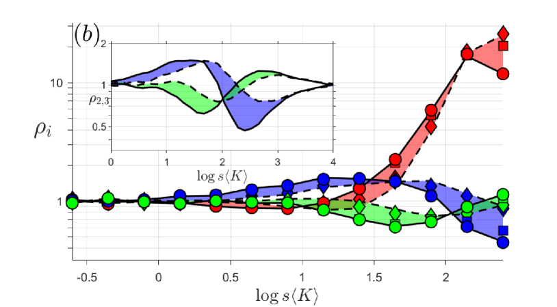
Figure 8: $\rho_{i}$ vs. $s\langle K\rangle$ for values of $s\in(10^{-3},1)$ and with $\langle K\rangle=250$ and $\gamma=0.8$ kept fixed, see text. (a) $\vec{r}=\vec{r}^{(1)}$; (b) $\vec{r}=\vec{r}^{(2)}$. Shaded areas and symbols are from stochastic simulations with $\nu=10$ ($\circ$), $\nu=0.1$ ($\square$), $\nu=10^{-5/2}$ ($\diamond$); lines show $\rho_{i}^{(\infty)}$ (fast switching, solid) and $\rho_{i}^{(0)}$ (slow switching, dashed), see text. Insets: (a) $\rho_{1}^{(\infty)}$ (solid) and $\rho_{1}^{(0)}$ (dashed) vs. $s\langle K\rangle$; (b) $\rho_{2}^{(\infty)}$ and $\rho_{3}^{(\infty)}$ (solid), $\rho_{2}^{(0)}$ and $\rho_{3}^{(0)}$ (dashed) vs. $s\langle K\rangle$ with $\gamma=0.8$ and $\langle K\rangle=10000$ fixed and $s$ varies between $1/\langle K\rangle$ and $1$. When $s\langle K\rangle=10^{3}-10^{4}$, $\rho_{i}\to 1$. In both panels and insets: species 1 in red, species 2 in blue, and species 3 in green; $\vec{x}_{0}=\vec{x}_{c}$; $\epsilon=0$.

In Fig. 8, we notice a non-monotonic dependence of $\rho_{i}$ on $s\langle K\rangle$ resulting from a different influence of environmental variability under weak and strong selection: In Fig. 8, the fixation probability of a species that is promoted/hindered under weak selection is hindered/promoted under strong selection.

4.2 Mean fixation time in the switching-$K$ BDCLV

In E.2, we analyze the effect of random switching on the mean extinction and absorption times $T_{1}$ and $T_{2}$ characterizing respectively the stages 1 and 2 of the switching-$K$ BDCLV dynamics, see Fig. S5(a,b). We thus show that, when $\vec{x}_{0}=\vec{x}_{c}$, the overall mean fixation time $T_{F}=T_{1}+T_{2}={\cal O}(\langle N\rangle)={\cal O}(\langle K\rangle)$ scales linearly with the average population size, see Fig. S5(c), similarly to $T_{F}$ in the constant-$K$ BDCLV. Hence, random switching makes the cyclic competition more “egalitarian” but does not prolong species coexistence. We also show that the average number of switches occurring in Stage 1 scales as $\nu\langle K\rangle$, see Fig. S6 (a), while the average number environmental switches along the edge $(i,i+1)$ in Stage 2 scales as ${\cal O}(\nu/\alpha_{i})$ when $s$ is neither vanishingly small nor too large.

5 Fixation properties of close-to-zero-sum rock-paper-scissors games in fluctuating populations

The general, non-zero-sum, rock-paper-scissors refers to the game with payoff matrix (2) where $\epsilon\neq 0$ and non-zero average fitness $\bar{f}=1-\epsilon\sum_{i=1}^{3}\alpha_{i}x_{i}x_{i+1}$. The mean-field description of the general RPS game, formulated as the birth-death process (6)-(2) with $0\leq s\leq 1/(1+\epsilon)$, is given by (see Sec. S1.1)

$$\dot{N} = N\left(\bar{f}-\frac{N}{K}\right)$$

$$\dot{x_{i}} = x_{i}[\alpha_{i}x_{i+1}-(1+\epsilon)\alpha_{i-1}x_{i-1}+1-\bar{f}].$$ (34)

In this model, the evolution of $N$ is coupled with the $x_{i}$’s, whose mean-field dynamics is characterized by heteroclinic cycles when $\epsilon>0$ and a stable coexistence fixed point when $\epsilon<0$  [20, 13, 14, 16, 17, 74, 18]

In this section, we briefly focus on the fixation probabilities of close-to-zero-sum rock-paper-scissors games when $|\epsilon|\ll 1$. We therefore approximate $\bar{f}\approx 1$ and still assume that there is a timescale separation between $N$ and $x_{i}$. This assumption is backed up by simulations results which also show that fixation properties are qualitatively the same as in the BDCLV, see Fig. 9 (to be compared with Figs. 4 and 7). This suggests that the fixation probabilities of close-to-zero-sum RPS games can be obtained from those of the BDCLV by rescaling the selection intensity according to $s\to s(1+\sigma\epsilon+{\cal O}(\epsilon^{2}))$, see Fig. 9.

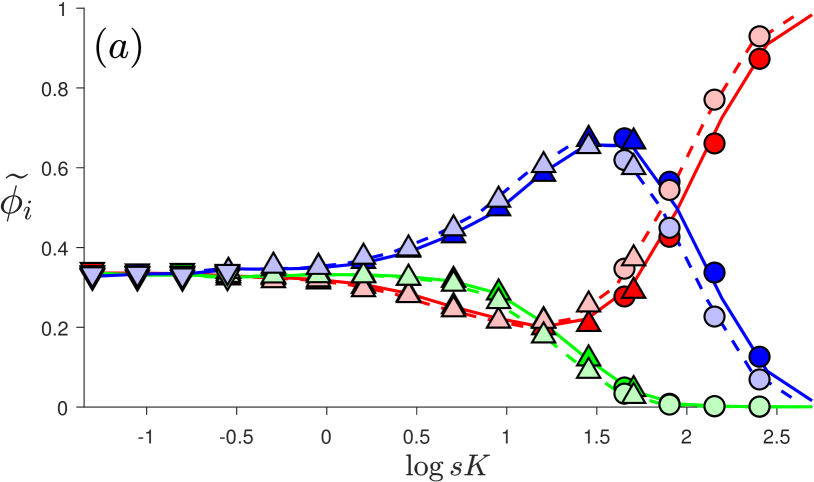
Figure 9: (a) ${\widetilde{\phi}}_{i}$ vs. $sK$ in the close-to-zero-sum RPS game with constant carrying capacity $K=450$ (circles), $90$ (upward triangles), $50$ (downward triangles), $\epsilon=-0.2$ (light symbols) and $\epsilon=0.2$ (dark symbols). Lines show stochastic simulation results for the BDCLV ($\epsilon=0$, see Fig. 4) with rescaled selection intensity $s\to s(1+\epsilon/2)$ with $\epsilon=0.2$ (solid) and $\epsilon=-0.2$ (dashed). Dark symbols / solid lines and light symbols / dashed lines collapse, demonstrating $\widetilde{\phi}_{i}^{\epsilon}(s)\simeq\widetilde{\phi}_{i}^{{\rm BDCLV}}(s(1+\epsilon/2))$, see text. (b) ${\widetilde{\phi}}_{i}$ vs. $s\langle K\rangle$ when $K$ switches between $K_{-}=50$ and $K_{+}=450$ ($\langle K\rangle=250,\gamma=0.8$), with $s\in(10^{-3},1)$. Symbols are stochastic simulation results for $\epsilon=-0.2$ and and $\nu=10$ (filled diamonds) and $\nu=0.001$ (open squares). Lines are stochastic simulation results from the BDCLV with same switching carrying capacity, $\nu=10$ (solid) and $\nu=0.001$ (dashed) and rescaled selection intensity $s\to s(1+\epsilon/2)$, see text and Fig. 7. (c) Same as in panel (b) with $\epsilon>0$: Symbols are stochastic simulation results for $\epsilon=0.2$; solid ($\nu=10$) and dashed ($\nu=0.001$) lines are results from the BDCLV with same switching carrying capacity and selection intensity $s\to s(1+\epsilon/2)$. In all panels: red denotes species 1, blue species 2, and green species 3; $\vec{r}=\vec{r}^{(1)}$ and $\vec{x}_{0}=\vec{x}_{c}$.

To determine the parameter $\sigma$, we consider the constant-$K$ RPS dynamics with $|\epsilon|\ll 1$. Since the fixation properties of the BDCLV vary little with the selection intensity at quasi neutrality and under strong selection, we focus on the regime (ii) of weak selection where $s\ll 1$ and $sK={\cal O}(10)$, and assume that $\phi_{ij}\approx 1/3$ and $P_{(i,j)}\approx 1$. As shown in C, the absorption probability of species $i$ along the edge $(i,i+1)$ in the realm of this approximation is

$$\phi_{i}\simeq\frac{e^{-\alpha_{i}(1+\frac{\epsilon}{2})K}+\alpha_{i}(1+\frac{\epsilon}{2})K-1}{\alpha_{i}(1+\frac{\epsilon}{2})K(1-e^{-\alpha_{i}(1+\frac{\epsilon}{2})K})},$$

which coincides with (16) upon rescaling the selection intensity according $s\to s(1+(\epsilon/2))$. Hence, if $\widetilde{\phi}_{i}^{\epsilon}(s)$ and $\widetilde{\phi}_{i}^{{\rm BDCLV}}(s)$ denote respectively the fixation probability of species $i$ in close-to-zero-sum RPS game with $|\epsilon|\ll 1$ and in the BDCLV, we have $\widetilde{\phi}_{i}^{\epsilon}(s)\simeq\widetilde{\phi}_{i}^{{\rm BDCLV}}(s(1+\epsilon/2))$. Since $\widetilde{\phi}_{i}$ is related to $\phi_{i}|_{K}$, via (18), the overall fixation probability is also obtained by rescaling the fixation probability $\widetilde{\phi}_{i}^{\rm BDCLV}$ with the same carrying capacity $K$ according to $s\to s(1+(\epsilon/2))$. This is confirmed by the results of Fig. 9 (a) where we find that this scaling holds across the regimes (i)-(iii).

This conclusion also holds when the carrying capacity $K(t)$ is randomly switching according to (5) and $|\epsilon|\ll 1$, see Fig. 9 (b,c). In fact, proceeding as above and focusing on the weak selection regime where $s\ll 1$ and $sK={\cal O}(10)$, we can assume $\phi_{ij}\approx 1/3$ and $P_{(i,j)}\approx 1$, and find that $\phi_{i}$ is given by (27) with the same carrying capacity $K(t)$ and a rescaled selection intensity $s\to s(1+(\epsilon/2))$. Along the same arguments as above, we expect that also when the carrying capacity is switching, the overall fixation probabilities across the regimes (i)-(iii) are approximately the same as in the switching-$K$ BDCLV subject to a rescaled selection intensity $s(1+(\epsilon/2))$. This is confirmed by the results of Fig. 9 (b,c) where we have reported $\widetilde{\phi}_{i}$ for fast and slow switching rates. As in the BDCLV, values of $\widetilde{\phi}_{i}$ for intermediate $\nu$ lie between the data shown in Fig. 9 (b,c).

In Section Sec. E.4, we show that the mean fixation time in the BDCLV with a rescaled selection intensity $s\to s(1+(\epsilon/2))$ allows us to obtain the mean fixation time of the close-to-zero-sum RPS game when $sK$ and $s\langle K\rangle$ are of order ${\cal O}(10)$ and $|\epsilon|\ll 1$.

6 Summary & Conclusion

Inspired by the evolution of microbial communities in volatile environments, we have studied the evolution three species engaged in a cyclic rock-paper-scissors competition when the environment varies randomly. In a static environment, the fixation probabilities in rock-paper-scissors games obey two different laws: The “law of the weakest” (LOW) prescribes that the species with the lowest payoff is the most likely to fixate in large populations, whereas a different rule (“law of stay out”, LOSO) arises in smaller populations [6, 4, 5, 33]. In this work, we have studied how this simple scenario changes when environmental and demographic noise are coupled. Environmental randomness is here introduced via a randomly switching carrying capacity (dichotomous Markov noise) modeling how the available resources switch continuously between states of scarcity and abundance.

We have studied a birth-and-death process, in which a fluctuating population of three species competing cyclically is subject to either a constant or randomly switching carrying capacity. As demographic fluctuations (internal noise) depend on the population size which in turn varies with the switching carrying capacity, internal and environmental noise are here coupled. The size of the fluctuating population can be subject to either the LOW (weak internal noise) or the LOSO (stronger internal noise), or can switch between values subject to one and then the other law. This can greatly influence the fixation properties: It is not clear which species will be the most likely to prevail when the population size fluctuates and how the outcome depends on the environmental variability. These questions have been studied in detail for the zero-sum rock-paper-scissors game, equivalent to the cyclic Lotka-Volterra model (CLV).

The CLV dynamics consists of two stages: Species coexist in Stage 1 until one of them dies out initiating Stage 2 that consists of a two-species competition. When the carrying capacity is constant, the CLV fixation probabilities under strong selection obey the LOW and the LOSO holds under weak selection. When the CLV is subject to a randomly switching carrying capacity, the fixation probabilities can be expressed in terms of the fixation probabilities of the CLV subject to a suitable constant carrying capacity. This has allowed us to analyze in detail how the variance and rate of change of the carrying capacity affect the fixation properties of the CLV. We have found that the general effect of random switching is to balance selection, and to “level the field” of the cyclic competition: When the average carrying capacity is kept constant, the species that is the least likely to fixate has a higher probability to prevail under random switching than in a static environment. In particular, we have shown that when the rate of switching is large, the effect of the environmental noise is to effectively reduce the selection strength by a factor increasing with the variance of the carrying capacity. Hence, when the carrying capacity has a large variance, the LOW becomes a zero-one-law only for much larger average population size than in the absence of switching. We have also found new fixation scenarios, not obeying neither the LOSO nor the LOW: Under determined conditions, one of the species surviving Stage 1 is best off below a critical switching rate, whereas the other is most likely to win under faster switching. Under random switching, fixation still occurs after a mean time that scales linearly with the average of the population size, with the subleading prefactor affected by the switching rate. Hence, environmental variability renders cyclic competition more “egalitarian” but does not prolong species coexistence. Finally, we have considered close-to-zero-sum rock-paper-scissors games and have shown that the fixation probabilities can be obtained from those of the CLV by a suitable rescaling of the selection intensity.

Acknowledgments

We thank Alastair Rucklidge for many helpful discussions. The support of an EPSRC PhD studentship (Grant No. EP/N509681/1) is gratefully acknowledged.

In this Supplementary Material (SM), we provide additional information about the relationships between various rock-paper-scissors models (Section A), and further technical details concerning the stages 1 and 2 dynamics (Section B and C). We also analyze the population composition at the inception of Stage 2 (Section D), as well as the mean extinction, absorption and fixation times (Section E) and discuss the average number of switches occurring in Stages 1 and 2. The notation in this SM is the same as in the main text; all equations not given in this SM refer to those of the main text.

Appendix A Various cyclic Lotka-Volterra models (zero-sum rock-paper-scissors games): general properties, similarities and differences

In the literature, there are various formulations of the zero-sum rock-paper-scissors games, here generically referred to as “cyclic Lotka-Volterra” models. Here, we consider the birth-death cyclic Lotka Volterra model (BDCLV), defined in the main text by (2)-(7), the cyclic Lotka Volterra model formulated in terms of a Moran process (MCLV), and finally the so-called chemical cyclic Lotka volterra model (cCLV). These models are characterized by many similar features, but also some important differences. Below, we outline some of the main properties of these models and discuss their similarities and differences.

A.1 The birth-death cyclic Lotka-Volterra model (BDCLV): Mean-field equations and piecewise deterministic Markov process

The BDCLV is here defined in terms of the six reactions

$$N_{i}\xrightarrow{T_{i}^{+}}N_{i}+1\quad\text{and}\quad N_{i}\xrightarrow{T_{i}^{-}}N_{i}-1,\quad\text{with}\quad i\in\{1,2,3\},$$ (S1)

the first set of reactions corresponds to the birth of an individual of species $i$ and the other reaction is associated with the death of an $i$-individual. These reactions occur with transition rates

$$T_{i}^{+}=f_{i}N_{i}=(1+s\Pi_{i})~{}N_{i}=(1+\{\alpha_{i}x_{i+1}-\alpha_{i-1}x_{i-1}\})~{}N_{i}\quad\text{and}\quad T_{i}^{-}=\frac{N}{K(t)}~{}N_{i},\quad\text{where}\;N=\sum_{i=1}^{3}N_{i}$$ (S2)

is the total population size and $K(t)$ is the carrying capacity. In this work, we consider the case of a constant and randomly switching carrying capacity, namely

$$K(t)=\begin{cases}K\quad\text{constant},&\mbox{ see Section 3}\\ \frac{1}{2}\left[\left(K_{+}+K_{-}\right)+\xi(t)\left(K_{+}-K_{-}\right)\right],\;\text{with dichotomous noise $\xi\in\{-1,+1\}$},&\mbox{ see Section 4 }\end{cases}.$$

The formulation of the cyclic competition in terms of the BDCLV allows us to conveniently introduce the carrying capacity through the death rate $T_{i}^{-}$ and, the population size not being conserved, also enables us to aptly model the cyclic dynamics when the population size fluctuates and possibly varies greatly in time.

The BDCLV dynamics is fully described by the underpinning master equation (7) from which the equation of motion of the average number of individual of species $i$ in the environmental state $\xi$ can be derived as usual [82, 83]

$$\frac{d}{dt}\langle N_{i}\rangle = \frac{d}{dt}\sum_{{\vec{N}}}N_{i}P(\vec{N},\xi,t)=\langle T_{i}^{+}\rangle-\langle T_{i}^{-}\rangle,\quad\text{where}$$

$$\langle T_{i}^{-}\rangle \equiv \begin{cases}\left\langle\frac{N}{K}~{}N_{i}\right\rangle&\mbox{, when $K$ is constant}\\ \left\langle T_{i}^{-}|_{+}\right\rangle=\left\langle\frac{N}{K_{+}}~{}N_{i}\right\rangle&\mbox{, in state $\xi=+1$ when $K$ is switching}\\ \left\langle T_{i}^{-}|_{-}\right\rangle=\left\langle\frac{N}{K_{-}}~{}N_{i}\right\rangle&\mbox{, in state $\xi=-1$ when $K$ is switching}\end{cases}.$$

This readily leads to the following equations for the average population size $\langle N\rangle$ in a static environment (constant $K$):

$$\frac{d}{dt}\langle N\rangle=\sum_{i=1}^{3}\left(\langle T_{i}^{+}\rangle-\langle T_{i}^{-}\rangle\right),\quad\text{and in a varying enviroment with a randomly switching $K$:}$$ (S3)

$$\frac{d}{dt}\langle N\rangle=\begin{cases}\sum_{i=1}^{3}\left(\langle T_{i}^{+}\rangle-\langle T_{i}^{-}|_{+}\rangle\right)&\mbox{if $\xi=+1$}\\ \sum_{i=1}^{3}\left(\langle T_{i}^{+}\rangle-\langle T_{i}^{-}|_{-}\rangle\right)&\mbox{if $\xi=-1$}\end{cases}.$$ (S4)

For the population composition, we can proceed similarly to derive the equation motion for $\langle x_{i}\rangle\equiv\langle N_{i}/N\rangle=\sum_{{\vec{N}}}(N_{i}/N)~{}P(\vec{N},\xi,t)$, paying due attention to the fact that now both $N_{i}$ and $N$ vary in time:

$$\frac{d}{dt}\langle x_{i}\rangle=\sum_{\vec{N}}\frac{N_{i}}{N}\frac{d}{dt}P(\vec{N},\xi,t)$$

$$= \sum_{\vec{N}}\frac{N_{i}}{N}\left\{T_{i}^{+}(\vec{N}-\vec{e}_{i})P(\vec{N}-\vec{e}_{i},\xi,t)+T_{i}^{-}(\vec{N}+\vec{e}_{i},K)P(\vec{N}+\vec{e}_{i},\xi,t)-\left(T_{i}^{+}(\vec{N})+T_{i}^{-}(\vec{N},K)\right)P(\vec{N},\xi,t)\right\}$$

$$+ \sum_{j\in\{1,2,3\}\neq i}\sum_{\vec{N}}\frac{N_{i}}{N}\left\{T_{j}^{+}(\vec{N}-\vec{e}_{j})P(\vec{N}-\vec{e}_{j},\xi,t)+T_{j}^{-}(\vec{N}+\vec{e}_{j},K)P(\vec{N}+\vec{e}_{j},\xi,t)-\left(T_{j}^{+}(\vec{N})+T_{j}^{-}(\vec{N},K)\right)P(\vec{N},\xi,t)\right\}$$

$$= \sum_{\vec{N}}\left\{\frac{N_{i}+1}{N+1}T_{i}^{+}(\vec{N})P(\vec{N},\xi,t)+\frac{N_{i}-1}{N-1}T_{i}^{-}(\vec{N},K)P(\vec{N},\xi,t)-\frac{N_{i}}{N}\left(T_{i}^{+}(\vec{N})+T_{i}^{-}(\vec{N},K)\right)P(\vec{N},\xi,t)\right\}$$

$$+ \sum_{j\in\{1,2,3\}\neq i}\sum_{\vec{N}}\left\{\frac{N_{i}}{N+1}T_{j}^{+}(\vec{N})P(\vec{N},\xi,t)+\frac{N_{i}}{N-1}T_{j}^{-}(\vec{N},K)P(\vec{N},\xi,t)-\frac{N_{i}}{N+1}\left(T_{j}^{+}(\vec{N})+T_{j}^{-}(\vec{N},K)\right)P(\vec{N},\xi,t)\right\},$$

where $\vec{e}_{i}$ is the unit vector such that $\vec{e}_{1}=(1,0,0)$, etc. By rearranging the right-hand-side of (A.1) and, for notational convenience, by writing $T^{+}\equiv T^{+}(\vec{N})$ and $T^{-}\equiv T^{-}(\vec{N},K)$, we obtain

$$\frac{d}{dt}\langle x_{i}\rangle = \left\langle\left(\frac{N_{i}+1}{N+1}-\frac{N_{i}}{N}\right)T_{i}^{+}\right\rangle+\left\langle\left(\frac{N_{i}-1}{N-1}-\frac{N_{i}}{N}\right)T_{i}^{-}\right\rangle+\sum_{j\in\{1,2,3\}\neq i}\left\{\left\langle\left(\frac{N_{i}}{N+1}-\frac{N_{i}}{N}\right)T_{j}^{+}\right\rangle+\left\langle\left(\frac{N_{i}}{N-1}-\frac{N_{i}}{N}\right)T_{j}^{-}\right\rangle\right\}$$ (S6)

$$= \left\langle\frac{T_{i}^{+}-T_{i}^{-}}{N}\left(1+{\cal O}\left(\frac{1}{N}\right)\right)\right\rangle-\left\langle\frac{x_{i}}{N}\left(1+{\cal O}\left(\frac{1}{N}\right)\right)~{}\sum_{j=1}^{3}\left(T_{j}^{+}-T_{j}^{-}\right)\right\rangle.$$

We can now derive the mean-field equations (constant $K$) and the stochastic differential equation (SDE) defining the piecewise-deterministic Markov process (PDMP) for the evolution of the population size. For this, as usual, we ignore all demographic fluctuations and factorize all terms appearing on the right-hand-side of (A.1) and (S6) in terms of $\langle x_{i}\rangle$ and $\langle N\rangle$, respectively denoted by $x_{i}$ and $N$, e.g. $\langle x_{i}x_{j}\rangle\to x_{i}x_{j},\langle f_{i}x_{j}N\rangle\to f_{i}x_{j}N$ and $\langle N_{i}N\rangle\to N_{i}N$. In the case of a constant carrying capacity, making the natural mean-field assumption that $N$ is always sufficiently large for contributions of order ${\cal O}(x_{i}/N)$ to be negligible, using (S3), we obtain:

$$\frac{d}{dt}N = \sum_{i=1}^{3}\left(T_{i}^{+}-T_{i}^{-}\right)=N\left(1-\frac{N}{K}\right),$$

$$\frac{d}{dt}x_{i} = \frac{T_{i}^{+}-T_{i}^{-}}{N}-x_{i}\left(\frac{dN/dt}{N}\right)=s\Pi_{i}x_{i}=x_{i}\left(\alpha_{i}x_{i+1}-\alpha_{i-1}x_{i-1}\right),$$ (S7)

where we have used $\bar{f}=1$ and $\alpha_{i}\equiv sr_{i}$. These mean-field equations coincide with the decoupled REs (9) and (10) discussed in the main text. In the case of a randomly switching carrying capacity, the $x_{i}$’s still obey (A.1) while the population size evolves according to

$$\frac{d}{dt}N=\begin{cases}N\left(1-\frac{N}{K_{+}}\right)&\text{if $\xi=+1$}\\ N\left(1-\frac{N}{K_{-}}\right)&\text{if $\xi=-1$,}\end{cases}$$ (S8)

which can be rewritten as the SDE (21) defining the PDMP governing the evolution of the population size $N(t)$ when demographic noise is ignored and whose stationary marginal probability density is given (22).

Similar derivations also hold in the general (non-zero-sum) rock-paper-scissors game, whose birth-death formulation is given by the rates $T_{i}^{\pm}$ of Eq. (7) and leads to the mean-field equations of Sec. 5.

A comment on our choice of the transition rates and of the model formulation is here in order: With (6) and (7) we have arguably chosen the simplest formulation of the RPS dynamics subject to a carrying capacity. It is however worth noting that other choices are of course also possible. Another natural possibility would be to use the transition rates $T_{i}^{+}=f_{i}N_{i}/\bar{f}$ and $T_{i}^{-}=(N/K)N_{i}$ [78]. Clearly, for the BDCLV these transition rates coincide with (7) since $\bar{f}=1$ when $\epsilon=0$. A difference however arises when $\epsilon\neq 0$ and $\bar{f}=1-\epsilon\sum_{i=1}^{3}\alpha_{i}x_{i}x_{i+1}$. In fact, proceeding as above and using the rates $T_{i}^{+}=f_{i}N_{i}/\bar{f}$ and $T_{i}^{-}=(N/K)N_{i}$ in the master equation (2), we obtain the following mean-field rate equations (MFREs): $\dot{N}=N(1-N/K)$ and $\dot{x}_{i}=x_{i}(f_{i}-\bar{f})/\bar{f}=x_{i}[\alpha_{i}x_{i+1}-(1+\epsilon)\alpha_{i-1}x_{i-1}+1-\bar{f}]/\bar{f}$. While these equations are decoupled, the MFREs for the $x_{i}$’s do not coincide with the celebrated replicator equations (5) of the general RPS game [14, 17]: The $x_{i}$’s MFREs obtained with the above alternative transition rates [13], differ from (5) due to the nonlinear $\bar{f}$ term appearing in the denominator on their right-hand-side. The MFREs $\dot{x}_{i}=x_{i}(f_{i}-\bar{f})/\bar{f}$ and Eqs. (5) however coincide to leading order in $s\epsilon$.

A.2 The Moran cyclic Lotka-Volterra model (MCLV)

We now outline the main features of the Moran cyclic Lotka Volterra model (MCLV) in a static environment (no environmental noise). The MCLV is defined by six pairwise reactions and is characterized by the conservation of the population size $N$ [78, 3, 79, 80, 15]. Each of the six reactions corresponds to the simultaneous death of an individual of species $i$ and the birth of an individual of species $j\neq i\in\{1,2,3\}$ [78]. This occurs with a rate $T_{i\to j}$. If the state of the system consisting of $N_{1}$ individuals of type $1$, $N_{2}$ of species $2$, and $N_{3}=N-N_{1}-N_{2}$ of the third type is denoted by $[N_{1},N_{2}]$, the six reactions of the MCLV are [67, 68, 69]

$$[N_{1},N_{2}]\xrightarrow{T_{1\to 2}}[N_{1}-1,N_{2}+1];\;[N_{1},N_{2}]\xrightarrow{T_{2\to 1}}[N_{1}+1,N_{2}-1]$$

$$[N_{1},N_{2}]\xrightarrow{T_{1\to 3}}[N_{1}-1,N_{2}];\;[N_{1},N_{2}]\xrightarrow{T_{3\to 1}}[N_{1}+1,N_{2}]$$

$$[N_{1},N_{2}]\xrightarrow{T_{2\to 3}}[N_{1},N_{2}-1];\;[N_{1},N_{2}]\xrightarrow{T_{3\to 2}}[N_{1},N_{2}+1],$$

with the transition rates [67, 68]

$$T_{j\to i}=f_{i}x_{i}x_{j}~{}N=(1+s\Pi_{i})~{}x_{i}x_{j}~{}N=(1+\{\alpha_{i}x_{i+1}-\alpha_{i-1}x_{i-1}\})~{}x_{i}x_{j}~{}N,$$ (S9)

where $f_{i}$ and $\Pi_{i}$ are given by (3) and (2). Interestingly, the transition rates of the MCLV can be expressed in terms of those of the BDCLV for a population of constant size $N=K$. In fact, using (S2) and $N=K$, we have $T_{j\to i}=T_{i}^{+}T_{j}^{-}/K$. This means that the BDCLV coincides with the MCLV in a population of constant size $N=K$, see below. Proceeding as above, we can readily find the mean-field rate equations for the MCLV:

$$\frac{d}{dt}x_{i}=\frac{1}{N}\sum_{j=1;j\neq i}^{3}\left(T_{j\to i}-T_{i\to j}\right)=s\Pi_{i}x_{i}=x_{i}\left(\alpha_{i}x_{i+1}-\alpha_{i-1}x_{i-1}\right),$$

which coincide with the mean-field (replicator) equations for the population composition in the BDCLV, see (A.1) and (10). Clearly therefore, in the constant-$K$ BDCLV the dynamics of the population composition coincides with that of the MCLV in the mean-field limit $K\to\infty$: both are characterized by the same neutrally stable fixed point $\vec{x}^{*}=(r_{2},r_{3},r_{1})=(r_{2},1-r_{1}-r_{2},r_{1})$ and constant of motion ${\cal R}=x_{1}^{r_{2}}x_{2}^{r_{3}}x_{3}^{r_{1}}$.

Since in the constant-$K$ BDCLV dynamics the population size obeys a logistic equation, after a short transient $N(t)\approx K$, see Eq. (9) and Fig. 1. This establishes a useful relationship between the BDCLV and MCLV: Except for a short transient (on a timescale $t\sim{\cal O}(1)$), corresponding to the so-called exponential phase of the logistic equation, the evolution of the constant-$K$ BDCLV is similar to the dynamics of the MCLV in a population of constant size $N=K$. The BDCLV and MCLV relation is particularly useful to determine the absorption/fixation properties of the former in terms of the well-studied fixation properties of latter, see Secs. 3.1.2 and C. In Fig. S1, we show that the survival and absorption probabilities $\phi_{i,j}$ and $\phi_{i}$ in the constant-$K$ BDCLV are almost indistinguishable from those obtained in the MCLV (with $N=K$). Since the overall fixation probabilities $\widetilde{\phi}_{i}=\phi_{i,i+1}\phi_{i}+\phi_{i-1,i}(1-\phi_{i})$, see Eq. (17), we can consider that the absorption and total fixation probabilities in the constant-$K$ BDCLV and those of the MCLV with $N=K\gg 1$ coincide. Similarly, the mean extinction and absorption times $T_{1}$ and $T_{2}$ in the BDCLV with constant-$K$ and MCLV with $N=K\gg 1$ are indistinguishable, see the insets of Fig. S1 and below.

To study the absorption/fixation properties of the BDCLV and MCLV, it is useful to write down the two-dimensional forward Fokker-Planck equation (FPE) obeyed by the probability density $P_{{\rm MCLV}}\equiv P_{{\rm MCLV}}(\vec{x},t)$ of the latter. Using standard methods, see, e.g. Refs. [82, 83, 19, 67, 68] we have the forward FPE

$$\left[\partial_{t}-{\cal G}_{{\rm fMCLV}}(\vec{x})\right]~{}P_{{\rm MCLV}}(\vec{x},t)=0,\quad\text{where}\quad{\cal G}_{{\rm fMCLV}}(\vec{x})\equiv-\sum_{i=1}^{2}\partial_{i}A_{i}^{{\rm MCLV}}(\vec{x})+\frac{1}{2}\sum_{i,j=1}^{2}\partial_{i}\partial_{j}B_{ij}^{{\rm MCLV}}(\vec{x}),\;$$ (S10)

is the forward FPE generator, with $\partial_{i}\equiv\partial/\partial x_{i}$ , defined by

$$A_{i}^{{\rm MCLV}}(\vec{x})\equiv\sum_{{j=1},j\neq i}^{3}\left(T_{j\to i}-T_{i\to j}\right);$$

$$B_{ii}^{{\rm MCLV}}(\vec{x})\equiv\sum_{{j=1},j\neq i}^{3}\left(\frac{T_{j\to i}+T_{i\to j}}{N}\right)\quad\text{and}\quad B_{12}^{{\rm MCLV}}(\vec{x})=B_{21}^{{\rm MCLV}}(\vec{x})\equiv-\left(\frac{T_{1\to 2}+T_{2\to 1}}{N}\right).$$ (S11)

Within the linear noise approximation [82, 83], upon linearising $A_{i}^{{\rm MCLV}}$ about the coexistence fixed point $\vec{x}^{*}$ and by evaluating $B_{ij}^{{\rm MCLV}}(\vec{x})$ at $\vec{x}^{*}$, in the variables $\vec{y}={\bf S}\vec{x}=\frac{\sqrt{3}}{2}\begin{pmatrix}\frac{(r_{1}+r_{2})\omega_{0}^{{\rm MCLV}}}{r_{1}r_{2}}&\frac{\omega_{0}^{{\rm MCLV}}}{r_{1}}\\ 0&1\end{pmatrix}~{}\vec{x}$, the forward FPE reads [19, 68]

$$\partial_{t}~{}P_{{\rm MCLV}}(\vec{y},t)=-\omega_{0}^{{\rm MCLV}}\left[y_{1}\partial_{y_{1}}-y_{2}\partial_{y_{2}}\right]~{}P_{{\rm MCLV}}(\vec{y},t)+D^{{\rm MCLV}}~{}[\partial_{y_{1}}^{2}+\partial_{y_{2}}^{2}]~{}P_{{\rm MCLV}}(\vec{y},t),$$ (S12)

where $\omega_{0}^{{\rm MCLV}}=s\sqrt{r_{1}r_{2}(1-r_{1}-r_{2})}$ and $D^{{\rm MCLV}}=3[r_{1}+r_{2}-4r_{1}r_{2}-(r_{1}-r_{2})^{2}]/(4N)$. To study the fixation properties of the MCLV, the FPEs (A.2) and (S12) have to be supplemented with absorbing boundaries at the corners of $S_{3}$ [19, 6, 33].

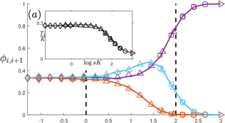
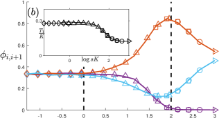
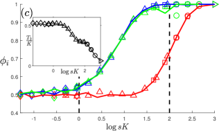
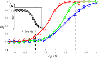
Figure S1: Comparison of the fixation properties vs. $sK$ in the BDCLV (solid lines) with constant carrying capacity $K$ and in the MCLV (symbols) with a constant population size $N=K\in\{1000~{}(\rhd),450~{}(\circ),250~{}(\diamond),90~{}(\square),50~{}(\triangle)\}$, with $\vec{r}=\vec{r}^{(1)}$ in (a,c) and $\vec{r}=\vec{r}^{(2)}$ in (b,d) and different values of selection intensity: $s\in\{10^{-j/4},j\in J_{K}^{\rm MCLV}\}$ with $J_{1000}^{\rm MCLV}=\{0\}$, $J_{450}^{\rm MCLV}=\{0,\dots,3\},J_{250}^{\rm MCLV}=\{0,\dots,4\},J_{90}^{\rm MCLV}=\{0,\dots,10\},J_{50}^{\rm MCLV}=\{7,\dots,12\}$ for the MCLV and $s\in\{10^{-j/4},j\in J_{K}^{\rm BDCLV}\}$ with $J_{1000}^{\rm BDCLV}=\{1\}$, $J_{450}^{\rm BDCLV}=\{0,\dots,12\},J_{90}^{\rm BDCLV}=\{10,11,12\},J_{50}^{\rm BDCLV}=\{12\}$ for the BDCLV. (a,b) Stage 1 survival probabilities $\phi_{1,2}$ (purple), $\phi_{2,3}$ (light blue) and $\phi_{3,1}$ (orange) vs. $sK$: BCLV results (lines) match perfectly with those obtained for the MCLV (symbols). Insets: Rescaled mean extinction times $T_{1}/K$ vs. $sK$ for the BDCLV (solid lines) and MCLV (symbols) virtually coincide, see text. (c,d) Stage 2 conditional fixation probabilities $\phi_{1}$ (red), $\phi_{2}$ (blue) and $\phi_{3}$ (green) vs. $sK$: BCLV results (lines) agree perfectly with those obtained for the MCLV (symbols). Insets: Rescaled mean absorption times $T_{2}/K$ vs. $sK$ for the BDCLV (solid lines) and MCLV (symbols) almost coincide, see text. In all panels: $\vec{x}_{0}=\vec{x}_{c}$, $\epsilon=0$; regimes (i)-(iii), from left to right, are indicatively separated by dashed lines. Simulation results for the fixation probabilities of in the constant-$K$ BDCLV and MCLV with $N=K$ are almost indistinguishable, see text.

A.3 The chemical cyclic Lotka-Volterra model (cCLV)

The chemical cyclic Lotka Volterra model (cCLV) is defined by three pairwise (“bimolecular”) reactions involving the simultaneous death and birth of individuals of different species, therefore conserving the total population size $N$. Hence, in the cCLV, in contrast to the BDCLV and MCLV, species $i$ is the predator of species $i+1$ and the prey of species $i-1$: an $i$-individual kills and replaces an $(i+1)$-individual with one of its offspring, while it is killed and replaced by individual of type $i-1$ according to the following “bimolecular chemical reactions”, with $N_{3}=N-N_{1}-N_{2}$:

$$12\xrightarrow{W_{2\to 1}}11\quad\text{(from state $[N_{1},N_{2}]$ to state $[N_{1}+1,N_{2}-1]$)}$$

$$23\xrightarrow{W_{3\to 2}}22\quad\text{(from state $[N_{1},N_{2}]$ to state $[N_{1},N_{2}+1]$)}$$

$$31\xrightarrow{W_{1\to 3}}33\quad\text{(from state $[N_{1},N_{2}]$ to state $[N_{1}-1,N_{2}]$).}$$

These reactions occur with the transition rates [19, 6, 33]

$$W_{i+1\to i}=k_{i}~{}\frac{N_{i}N_{i+1}}{N}=k_{i}x_{i}x_{i+1}~{}N,\quad\text{where $k_{i}\geq 0$.}$$ (S14)

Clearly, the reactions (A.3) and transition rates (S14) differ from those of the BDCLV and MCLV. Yet, as discussed below many of the features of the BDCLV, MCLV and cCLV are similar. The cCLV mean-field equations for the $x_{i}$’s are given by

$$\frac{d}{dt}x_{i}=\frac{W_{i+1\to i}-W_{i\to i-1}}{N}=x_{i}\left(k_{i}x_{i+1}-k_{i-1}x_{i-1}\right).$$ (S15)

We notice that upon rescaling the time as $t\to st/(k_{1}+k_{2}+k_{3})$, the reaction rates become $k_{i}\to k_{i}/(k_{1}+k_{2}+k_{3})=r_{i}$ and Eq. (S15) is identical to Eq. (A.1). Hence, upon time rescaling, the MCLV and cCLV are identical at mean-field level and their dynamics coincide with the REs (10) of the BDCLV. Moreover, Eqs. (A.1) and (A.2) admit the same marginally stable coexistence fixed point $\vec{x}^{*}=(k_{2},k_{3},k_{1})/(k_{1}+k_{2}+k_{3})=(r_{2},r_{3},r_{1})$ and the same constant of motion ${\cal R}=\left(x_{1}^{k_{2}}x_{2}^{k_{3}}x_{3}^{k_{1}}\right)^{1/(k_{1}+k_{2}+k_{3})}$. The mean-field dynamics of the $x_{i}$’s is therefore identical for the BDCLV, MCLV and cCLV.

It is useful to proceed as above and consider the two-dimensional forward Fokker-Planck equation (FPE) obeyed by the cCLV probability density $P_{{\rm cCLV}}\equiv P_{{\rm cCLV}}(\vec{x},t)$ (with $t\to t/N$):

$$\left[\partial_{t}-{\cal G}_{{\rm cCLV}}(\vec{x})\right]~{}P_{{\rm cCLV}}(\vec{x},t)=0,\quad\text{where}\quad{\cal G}_{{\rm cCLV}}(\vec{x})\equiv-\sum_{i=1}^{2}\partial_{i}A_{i}^{{\rm cCLV}}(\vec{x})+\frac{1}{2}\sum_{i,j=1}^{2}\partial_{i}\partial_{j}B_{ij}^{{\rm cCLV}}(\vec{x}),\;$$ (S16)

with $A_{i}^{{\rm cCLV}}(\vec{x})\equiv W_{i+1\to i}-W_{i\to i-1}$, $B_{ii}^{{\rm cCLV}}(\vec{x})\equiv\left(W_{i+1\to i}+W_{i\to i-1}\right)/N$ where $i\in\{1,2\}$, and $B_{12}^{{\rm cCLV}}(\vec{x})=B_{21}^{{\rm cCLV}}(\vec{x})\equiv-(W_{1\to 2}+W_{2\to 1})/N$. It is worth noting that the drift terms of the cCLV and MCLV are simply related by $A_{i}^{{\rm cCLV}}=sA_{i}^{{\rm MCLV}}/(k_{1}+k_{2}+k_{3})$. In the case of symmetric rates, $k_{1}=k_{2}=k_{3}=1$, within the linear noise approximation, this forward FPE in the variables $\vec{y}={\bf S}\vec{x}$ reads:

$$\partial_{t}~{}P_{{\rm cCLV}}(\vec{y},t)=-\omega_{0}^{{\rm cCLV}}\left[y_{1}\partial_{y_{1}}-y_{2}\partial_{y_{2}}\right]~{}P_{{\rm cCLV}}(\vec{y},t)+D^{{\rm cCLV}}~{}[\partial_{y_{1}}^{2}+\partial_{y_{2}}^{2}]~{}P_{{\rm cCLV}}(\vec{y},t),$$ (S17)

where $\omega_{0}^{{\rm cCLV}}=1/\sqrt{3}$ and $D^{{\rm cCLV}}=1/(12N)$ [19]. This FPE is similar to Eq. (A.2). The comparison with the MCLV with equal rates $r_{i}=1/3$ is particularly illuminating: $\omega_{0}^{{\rm MCLV}}=s\omega_{0}^{{\rm cCLV}}/3$ and $D^{{\rm MCLV}}=2D^{{\rm cCLV}}$. Hence, upon a suitable rescaling of the timescale, the MCLV and cCLV deterministic drift and diffusive terms (about $\vec{x}^{*}$) can be mapped onto each other.

A.3.1 Fixation probabilities in the cCLV: The law of the weakest and the law of stay out

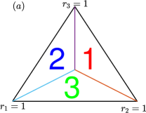
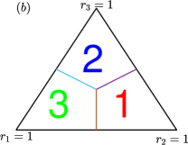
Figure S2: Law of the weakest (a) and law of stay out (b) in the simplex $S_{3}$ spanned by $r_{i}$, divided into three regions where the most likely species to survive is labelled. On the lines separating these regions, both adjacent species are equally likely to survive. (a) Law of the weakest (LOW): In the cCLV, the most likely species to survive in a large population is that with the lowest $r_{i}$. The LOW becomes asymptotically a zero-one law and also applies to the constant-$K$ BDCLV and MCLV when $N=K$ and $sK\gg 1$ (regime (iii)), see text. (b) Law of stay out (LOSO) when all species initially coexist with the same density: In the cCLV, no species is guaranteed to survive is small populations, see text. The LOSO also applies to the constant-$K$ BDCLV and MCLV when $N=K$ and $sK={\cal O}(10)$ (regime (ii)), see text.

Due to the predator-prey interactions underpinning the cCLV, its fixation properties of the cCLV are entirely set by the stage 1 of its dynamics: the probability $\phi_{i,i+1}^{{\rm cCLV}}$ that species $i$ and $i+1$ survive the stage 1 coincides with the fixation probability $\phi_{i}^{{\rm cCLV}}$ of species $i$: $\phi_{i,i+1}^{{\rm cCLV}}=\phi_{i}^{{\rm cCLV}}$. The survival/fixation probability $\phi_{i}^{{\rm cCLV}}$ of the cCLV can be explained by two simple laws called the law of the weakest (LOW) and the law of stay out (LOSO) [6, 4, 23, 33], see Fig.S2. The former applies to populations of large size and the latter to small populations. The LOW says that in a sufficiently large population (when $N\gtrsim 10^{2}$) evolving according to the cCLV, the most likely species to survive is the one with the lowest rate $k_{i}$ [6] ($i\in\{1,2,3\}$), see Fig.S2 (a):

$$\phi_{i}^{{\rm cCLV}}>\phi_{i+1}^{{\rm cCLV}},\phi_{i-1}^{{\rm cCLV}}\;\text{if \quad$k_{i}<k_{i\pm 1},\;\;\;$ and \;\;\; $\phi_{i}^{{\rm cCLV}}\approx\phi_{i+1}^{{\rm cCLV}}>\phi_{i-1}^{{\rm cCLV}}\;$ if $\quad k_{i}=k_{i+1}<k_{i-1},\;$ with $\;i\in\{1,2,3\}$. }$$ (S18)

The LOW becomes asymptotically a zero-one law (when $N\gtrsim 10^{3}$):

$$\phi_{i}^{{\rm cCLV}}\to 1,\phi_{i\pm 1}\to 0\quad\text{if $k_{i}<k_{i\pm 1}$, \quad while \quad$\phi_{i}^{{\rm cCLV}}=\phi_{i+1}^{{\rm cCLV}}\to 1/2$ and $\phi_{i-1}^{{\rm cCLV}}\to 0$ if $k_{i}=k_{i+1}<k_{i-1}$.}$$ (S19)

The LOW is independent of the initial condition and results from the fact that in large populations, due to the effect of weak demographic noise the cCLV trajectories perform random walks between the deterministic orbits until they reach the so-called “outermost orbit”. This is obtained from the constant of motion ${\cal R}$ as the deterministic orbit that lies at a distance $1/N$ from the closest edge of $S_{3}$ [6, 33]. In the cCLV, the extinction of a first species occurs when a chance fluctuation pushes a trajectory along the edge of $S_{3}$ from where the absorbing state corresponding to the fixation of the “weakest species” (with lowest $k_{i}$) and death of its “prey” is attained exponentially quickly.

The LOSO is a non-zero-one law prescribing which species is most likely to survive in small populations ($3\leq N\lesssim 50$). The LOSO results from the interplay between the deterministic drift and demographic fluctuations and its prescriptions depend on the initial condition. In the cCLV, when initially all species have the same density, i.e. $\vec{x}_{0}=\vec{x}_{c}$, the LOSO says that the most likely species to survive is/are the one(s) predating on the species with the highest $k_{i}$’s, see Fig.S2 (b) [6, 33]:

$$\phi_{i-1}^{{\rm cCLV}}>\phi_{i}^{{\rm cCLV}},\phi_{i+1}^{{\rm cCLV}}\quad\text{if $\quad k_{i}>k_{i+1},k_{i-1}$, \quad and \quad}\phi_{i}^{{\rm cCLV}}\approx\phi_{i+1}^{{\rm cCLV}}>\phi_{i-1}^{{\rm cCLV}}\quad\text{if $\quad k_{i+1}=k_{i-1}>k_{i}$}.$$ (S20)

The LOSO can be understood by estimating the initial drift at $\vec{x}_{0}$ with the Jacobian $\bf{J}^{*}$ of (S15) evaluated at $\vec{x}^{*}$. When, as here, $\vec{x}_{0}\neq\vec{x}^{*}$, the rate of the bias from $\vec{x}_{0}$ towards a corner $i$ of $S_{3}$ is $({\bf J}^{*}\vec{x}_{0})_{i}=k_{i}x_{i+1}(0)-k_{i-1}x_{i-1}(0)$. Hence, $k_{i}^{-}\equiv k_{i}x_{i+1}(0)-k_{i-1}x_{i-1}(0)$, gives the initial deterministic rate in the direction $i$. The most likely species to die out first is therefore the one with the smallest $k_{i}^{-}$ (edge $(i-1,i+1)$ as the most likely to be hit first). With this reasoning, and $k_{i}^{-}=(k_{i}-k_{i-1})/3$ when $\vec{x}_{0}=\vec{x}_{c}$, we find that the species that is the least likely to survive/fixate in the cCLV satisfies (S20) when all species initially coexist with the same density $x_{i}(0)=1/3$.

A.3.2 Mean extinction and fixation times in the cCLV

The cCLV dynamics is also characterized by two stages: in Stage 1, the three species coexist until an edge of $S_{3}$ is hit and one of the species dies out (see Sec. 3.1.1) after a mean extinction time $T_{1}^{{\rm cCLV}}={\cal O}(N)$, see Sec. E.1.1. While the stage 1 dynamics of the cCLV, MCLV and constant-$K$ BDCLV are similar (when $s={\cal O}(1)$), a major difference arises in Stage 2, when two species, say $i$ and its weak opponent $i+1$, compete along the edge $(i,i+1)$ of $S_{3}$. According to the cCLV, the interaction between species $i$ (predator) and $i+1$ (prey) is of predator-prey type, and the outcome of Stage 2 is certain: Contrarily to the MCLV and BDCLV, species $i$ always wins against $i+1$ exponentially quickly in time. The overall cCLV mean fixation time $T_{F}^{{\rm cCLV}}=T_{1}^{{\rm cCLV}}+T_{2}^{{\rm cCLV}}$ therefore coincides with $T_{1}^{{\rm cCLV}}$ to leading order, yielding $T_{F}^{{\rm cCLV}}\simeq T_{1}^{{\rm cCLV}}={\cal O}(N)$, when $N\gg 1$ [19, 25, 33].

It has been shown that the mean extinction/fixation time $T_{1}^{{\rm cCLV}}$ can be obtained from the linear approximation about $\vec{x}^{*}$ [19] (see also [68, 28]). For this, it is useful to consider the FPE (S17) in polar coordinates, via $y_{1}=r\cos{\theta}$ and $y_{2}=r\sin{\theta}$. Since there is no angular dependence when $\vec{x}_{0}=\vec{x}^{*}$, one has $P_{{\rm cCLV}}(\vec{y},t)\to P_{{\rm cCLV}}(r,t)$ with

$$\partial_{t}~{}P_{{\rm cCLV}}(r,t)=D^{{\rm cCLV}}~{}[r^{-1}\partial_{r}+\partial_{r}^{2}]~{}P_{{\rm cCLV}}(r,\theta,t),$$ (S21)

which is the two-dimensional diffusion equation in polar coordinates with only radial dependence and diffusion constant $D^{{\rm cCLV}}=1/(12N)$. By supplementing this FPE with an absorbing boundary at $\partial S_{3}$, approximated as a circle of radius $R$ in order to exploit the symmetry about $\vec{x}^{*}$, the mean extinction time was found to scale with $N$:

$$T_{1}^{{\rm cCLV}}\simeq 3R^{2}~{}N,\quad\text{where}\quad R=\frac{1}{2\sqrt{3}}\left(1+\frac{1}{\sqrt{3}}\right).$$ (S22)

Hence, in the cCLV with equal rates ($k_{i}=1$), the mean fixation and extinction time when the dynamics starts at $\vec{x}^{*}$ is $T_{F}^{{\rm cCLV}}\simeq T_{1}^{{\rm cCLV}}\simeq 0.62N$. Qualitatively, the same conclusion $T_{F}^{{\rm cCLV}}\simeq T_{1}^{{\rm cCLV}}={\cal O}(N)$ also holds when the rates $k_{i}$ are unequal [19].

Appendix B Stage 1 dynamics in the constant-$K$ BDCLV and MCLV: similarities with the cCLV

We have seen that the cCLV survival/fixation probabilities are set in Stage 1 by the outermost orbit and follow the LOW in large populations. The MCLV and cCLV obey the same mean-field equations (up to time rescaling), with the same constant of motion ${\cal R}$ and fixed points, see Eqs. (S15) and (A.2), and as such they admit the same outermost orbits. Furthermore, with the same timescale, the diffusion constant in the MCLV is $1/(Ns)$ and $1/N$ in the cCLV. The survival probabilities $\phi_{i,i+1}^{{\rm MCLV}}$ of a population evolving with the MCLV are therefore expected to correspond to those of the cCLV in a population of effective size ${\cal O}(Ns)$, with rates related according to $r_{i}=k_{i}/(k_{1}+k_{2}+k_{3})$. We have also seen that in the constant-$K$ BDCLV the population size rapidly fluctuates about $K$, i.e. $N(t)\simeq K$, see Eq. (10) and Fig. 1, and its survival probabilities are the same as in the MCLV with $N=K\gg 1$, see Fig. S1. The survival probabilities $\phi_{i,i+1}$ in the constant-$K$ BDCLV are therefore the same as those, $\phi_{i,i+1}^{{\rm cCLV}}|_{Ks}$, in the cCLV with a population of size ${\cal O}(Ks)$: $\phi_{i,i+1}\approx\phi_{i,i+1}^{{\rm MCLV}}|_{K}\approx\phi_{i,i+1}^{{\rm cCLV}}|_{Ks}=\phi_{i}^{{\rm cCLV}}|_{Ks}$. We therefore expect that the survival probabilities of the constant-$K$ BDCLV obey the LOW when $Ks\gtrsim 100$, whereas they obey the LOSO when $Ks={\cal O}(10)$, see Fig. S2. This is confirmed by the results discussed in Sec. 3.1.1, see Fig. 3 (a,b). We have also seen that the mean extinction time in the cCLV scales with $N$ to leading order and can be obtained within a linear noise approximation about $\vec{x}^{*}$. We can proceed similarly with the MCLV, and since the linear noise approximation about $\vec{x}^{*}$ of the cCLV and MCLV is similar, see Eqs. (S17) and (A.2), we can obtain the mean extinction time $T_{1}^{\rm MCLV}$ by solving the radial diffusion equation $\partial_{t}~{}P_{{\rm MCLV}}(r,t)=D^{{\rm MCLV}}~{}[r^{-1}\partial_{r}+\partial_{r}^{2}]~{}P_{{\rm MCLV}}(r,\theta,t)$, with absorbing boundary on $\partial S_{3}$ and $D^{{\rm MCLV}}=2D^{{\rm cCLV}}$. This yields $T_{1}^{\rm MCLV}\simeq\frac{3}{2}R^{2}N\approx 0.3N$ when $r_{i}=r=1/3$ (symmetric rates). A similar relation, with a different expression of $R$, holds when the rates $r_{i}$ are asymmetric. Since $N(t)\simeq K$ in the constant-$K$ BDCLV (after a time $t={\cal O}(1)$), we readily obtain its mean extinction time: $T_{1}\simeq\frac{3}{2}R^{2}K\approx 0.3K$ to leading order in $K\gg 1$, when $r_{i}=1/3$. The insets of Fig. S1 confirm that $T_{1}$ in constant-$K$ BDCLV is almost indistinguishable from $T_{1}^{\rm MCLV}$ obtained in the MCLV with $N=K\gg 1$. This result also holds when the dynamics towards extinction is driven by diffusion (weak demographic noise). This is certainly the case when $\vec{x}_{0}=\vec{x}^{*}$ and also when $\vec{x}_{0}\neq\vec{x}^{*}$ and $s\ll 1$. In fact, under weak selection, the deterministic drift arising when $\vec{x}_{0}\neq\vec{x}^{*}$ is weak and extinction is driven by weak demographic fluctuations when $s\ll 1$. we therefore find $T_{1}\simeq\frac{3}{2}R^{2}N\approx 0.3N$ when $r_{i}=r=1/3$ and when $s\ll 1$ and $sK={\cal O}(1)$, as reported in Fig. S4(a).

Appendix C Stage 2 dynamics in a population with constant carrying capacity

In stark contrast to the cCLV, the outcome of Stage 2 in the MCLV/BDCLV is not certain. This is because the interactions in the MCLV/BDCLV are not of predator-prey type: In Stage 2, the dynamics boils down to the competition between species $i$ and its “weak opponent”, species $i+1$, that the latter has a non-zero chance to win it.

To study this two-species competition, we focus on the stage 2 dynamics along the edge $(i,i+1)$. Since species $i-1$ has died out at the end of Stage 1, we have $x_{i}+x_{i+1}=1$ and $x_{i-1}=0$, and the constant-$K$ BDCLV transition rates in Stage 2 are $T_{j}^{+}=(1+s\Pi_{j})~{}Nx_{j}$ and $T_{j}^{-}=N^{2}x_{j}/K$, with $j\in\{i,i+1\}$, see (S2). Similarly, the transition rates of the MCLV along the edge $(i,i+1)$ for a population of size $N=K$ are obtained from (S9) with $x_{i+1}=1-x_{i}$ and $x_{i-1}=0$:

$$T_{i+1\to i}=\frac{T_{i}^{+}T_{i+1}^{-}}{K}=Kx_{i}(1-x_{i})(1+\alpha_{i}(1-x_{i}))\quad\text{and}\quad T_{i\to i+1}=\frac{T_{i}^{-}T_{i+1}^{+}}{K}=Kx_{i}(1-x_{i})(1-\alpha_{i}x_{i}).$$ (S23)

It is clear from these transition rates that, $x_{i}=0,1$ are the possible outcome of the stage 2 dynamics and correspond to either the absorption of species $i$ with probability $\phi_{i}|_{K}$ ($x_{i}=1,x_{i+1}=0$), or the the absorption of $i+1$ ($x_{i}=0,x_{i+1}=1$) with probability $1-\phi_{i}|_{K}$.

Clearly, (S23) define a one-dimensional Moran process whose fixation properties can be computed exactly [3, 80]. For our purposes, the diffusion theory allows us to obtain a concise and reliable characterization of $\phi_{i}|_{K}$. In fact, the backward version of the FPE generator (S10) for the MCLV (with $N=K$) along the edge $(i,i+1)$ is [82, 83]

$${\cal G}|_{K}(x_{i})\equiv\frac{x_{i}(1-x_{i})}{K}\left[K\alpha_{i}\frac{\partial}{\partial x_{i}}+\left\{1+\frac{\alpha_{i}}{2}(1-2x_{i})\right\}\frac{\partial^{2}}{\partial x_{i}^{2}}\right].$$

When Stage 2 starts with a fraction $\hat{x}_{i}$ of individuals of species $i$, the fixation probability $\phi_{i}|_{K}$ of the underpinning MCLV is obtained in the realm of the diffusion theory by solving ${\cal G}|_{K}(\hat{x}_{i})~{}\phi_{i}|_{K}(\hat{x}_{i})=0$ with $\phi_{i}|_{K}(0)=0$ and $\phi_{i}|_{K}(1)=1$. This yields

$$\phi_{i}|_{K}(\hat{x}_{i})=\frac{(2+\alpha_{i})^{K+1}-\left\{2+\alpha_{i}(1-2\hat{x}_{i})\right\}^{K+1}}{(2+\alpha_{i})^{K+1}-(2-\alpha_{i})^{K+1}}.$$

When $s\ll 1$, i.e. $\alpha_{i}\ll 1$, the backward FPE generator takes the classical form [2, 3, 79]

$${\cal G}|_{K}(x_{i})=\frac{x_{i}(1-x_{i})}{K}\left[K\alpha_{i}\frac{\partial}{\partial x_{i}}+\frac{\partial^{2}}{\partial x_{i}^{2}}\right],\quad\text{yielding the familiar expression}\quad\phi_{i}|_{K}(\hat{x}_{i})=\frac{1-e^{-\alpha_{i}K~{}\hat{x}_{i}}}{1-e^{-\alpha_{i}K}}.$$ (S24)

In the realm of the diffusion theory, the MCLV mean absorption time $T_{2}^{{\rm MCLV}}$ (from the inception of Stage 2) with an initial fraction $\hat{x}_{i}$ of $i$ individuals, $T_{2}^{{\rm MCLV}}(\hat{x}_{i})$, is obtained from the FPE generator ${\cal G}_{(i,i+1)}|_{K}$ by solving ${\cal G}|_{K}(\hat{x}_{i})T_{2}^{{\rm MCLV}}(\hat{x}_{i})=-1$ with boundary conditions $T_{2}^{{\rm MCLV}}(\hat{x}_{i}=0)=T_{2}^{{\rm MCLV}}(\hat{x}_{i}=1)=0$ [82, 83, 3, 2]. The insets of Fig. S1 confirm that the mean absorption time $T_{2}^{(i,i+1)}$ along the edge $(i,i+1)$ in the constant-$K$ BDCLV virtually coincide with $T_{2}^{{\rm MCLV}}$ when $N=K\gg 1$: $T_{2}^{(i,i+1)}\simeq T_{2}^{{\rm MCLV}}$. The FPE for $T_{2}^{{\rm MCLV}}$ can be solved by standard methods and generally yields a cumbersome expression. In the limit of weak selection, $s\ll 1$, we can use the simpler form (S24) and find that $T_{2}^{(i,i+1)}\simeq T_{2}^{{\rm MCLV}}\sim(\log{K})/s$ when $s\ll 1$ and $sK\gg 1$. In this case, $T_{2}^{(i,i+1)}$ scales as $1/s$ to leading order, with a subleading dependence on the population size via the prefactor $\log{K}$. When $s\ll 1$ and $sK\lesssim 1$, $T_{2}^{(i,i+1)}={\cal O}(K)$ at quasi-neutrality, while $T_{2}^{(i,i+1)}\sim\log{K}$ when $sK\gg 1$ (strong selection), as shown in Fig. S4 (b).

A similar analysis can be carried out when $\epsilon>0$, see Section 5. In this case, the non-zero-sum birth-death dynamics defined by (7) with constant carrying capacity $K\gg 1$ is similar to the dynamics of Moran model defined by the transition rates

$$T_{i+1\to i}=\frac{T_{i}^{+}T_{i+1}^{-}}{K}=Kx_{i}(1-x_{i})(1+\alpha_{i}(1-x_{i}))\quad\text{and}\quad T_{i\to i+1}=\frac{T_{i}^{-}T_{i+1}^{+}}{K}=Kx_{i}(1-x_{i})(1-\alpha_{i}(1+\epsilon)x_{i}).$$ (S25)

in a population of constant size $N=K$. In this case, the stage 2 dynamics along the edge $(i,i+1)$ is characterized by the backward FPE generator ${\cal G}^{\epsilon}|_{K}(x_{i})\equiv\frac{x_{i}(1-x_{i})}{K}\left[K\alpha_{i}(1+\epsilon x_{i})\partial_{i}+\left\{1+\frac{\alpha_{i}}{2}(1-(2+\epsilon)x_{i})\right\}\partial_{i}^{2}\right]$. The absorption probability is thus obtained by solving ${\cal G}^{\epsilon}|_{K}(\hat{x}_{i})\phi_{i}|_{K}(\hat{x}_{i})=0$ with $\phi_{i}|_{K}(0)=1-\phi_{i}|_{K}(1)=0$ yielding

$$\phi_{i}|_{K}(\hat{x}_{i})=\frac{(2+\alpha_{i})^{Kh(\epsilon,\alpha_{i})+1}-\left\{2+\alpha_{i}(1-(2+\epsilon)\hat{x}_{i})\right\}^{Kh(\epsilon,\alpha_{i})+1}}{(2+\alpha_{i})^{Kh(\epsilon,\alpha_{i})+1}-(2-\alpha_{i}(1+\epsilon))^{Kh(\epsilon,\alpha_{i})+1}},\quad\text{where}\quad h(\epsilon,\alpha_{i})\equiv\frac{1+\epsilon(1+1/\alpha_{i})}{(1+\epsilon/2)^{2}}.$$ (S26)

When $|\epsilon|\ll 1$, this expression simplifies in the weak selection regime ($s\ll 1$) where it takes the form

$$\phi_{i}|_{K}(\hat{x}_{i})\simeq\frac{1-e^{-K\alpha_{i}(1+\epsilon/2)\hat{x}_{i}}}{1-e^{-K\alpha_{i}(1+\epsilon/2)}}.$$ (S27)

Hence, the stage 2 fixation probability in the weak selection regime when $|\epsilon|\ll 1$ is the same as in the constant-$K$ BDCLV with a selection intensity is rescaled by a factor $1+\epsilon/2$ ($s\to s(1+\epsilon/2)$). This suggests to consider the following effective backward FPE generator when $s\ll 1$ and $|\epsilon|\ll 1$: ${\cal G}^{\epsilon}|_{K}(x_{i})\equiv\frac{x_{i}(1-x_{i})}{K}\left[K\alpha_{i}(1+\epsilon/2)~{}\partial_{i}+\partial_{i}^{2}\right]$. In this case, the mean absorption time is given ${\cal G}^{\epsilon}|_{K}(\hat{x}_{i})T_{2}(\hat{x}_{i})=-1$ with $T_{2}(\hat{x}_{i}=0)=T_{2}(\hat{x}_{i}=1)=0$. Clearly, this implies that the mean absorption time is obtained from $T_{2}$ of the constant-$K$ BDCLV with a rescaled selection intensity $s\to s(1+\epsilon/2)$. We have checked in our simulations that this rescaling also applies to Stage 1 and therefore to the overall mean fixation time, see E.4 and Fig. S6 (b)-(d).

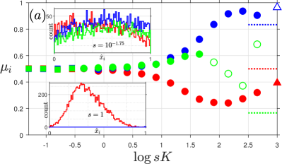
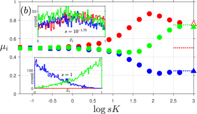
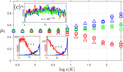
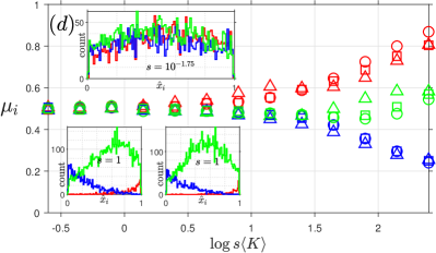
Figure S3: Population composition at the inception of Stage 2 vs. $sK$ (a,b) and $s\langle K\rangle$ (c,d) with $\vec{r}=\vec{r}^{(1)}$ in (a,c) and $\vec{r}=\vec{r}^{(2)}$ in (b,d). In all panels: $\mu_{i}=\int_{0}^{1}\hat{x}_{i}P_{(i,i+1)}(\hat{x}_{i})~{}d\hat{x}_{i}$ is the mean value of $\hat{x}_{i}$ for species $i=1$ (red), $2$ (blue), $3$ (green), with $\vec{x}_{0}=\vec{x}_{c}$ and $\epsilon=0$. (a,b) $\mu_{i}$ vs. $sK$ in the constant-$K$ BDCLV with $K=1000~{}(\triangle),450~{}(\circ),50~{}(\square)$ and $s\in(10^{-3},1)$. (Empty symbols denote data arising from small survival probability $\phi_{i,i+1}<0.01$ that would require additional sampling). When $sK\lesssim 10$, $\mu_{i}\approx 1/2$ and $P_{(i,i+1)}\approx 1$ is approximately uniform. When $sK\gg 1$, the dynamics is dominated by the LOW and $\mu_{i}\approx r_{i+1}/(r_{i+1}+r_{i-1})$ shown as dotted lines, see text. Upper insets: Histograms corresponding to $P_{(i,i+1)}(\hat{x}_{i})$ with $s=10^{-7/4}$ and $K=250$, is approximately uniform, corresponding to $P_{(i,i+1)}\approx 1$, along the three edges. Lower insets: Same with $s=1$ and $K=1000$, showing that $P_{(i,i+1)}$ is no longer uniform when $sK\gg 1$ and how it changes with $\nu=10$ (left) and $\nu=0.1$ (right). (c,d) $\mu_{i}$ vs. $s\langle K\rangle$ in the switching-$K$ BDCLV with $\langle K\rangle=250$ and $\gamma=0.8$ kept fixed and $s$ varies with $\nu=10~{}(\square)$, $\nu=1~{}(\circ)$ and $\nu=0.001~{}(\triangle)$. Insets: (Upper) Histograms corresponding to $P_{(i,i+1)}(\hat{x}_{i})$ with $s=10^{-7/4}$, $\nu=0.1$ and $\langle K\rangle=250,\gamma=0.8$ for $i=1,2,3$. (Lower) Same with $s=1$, $\langle K\rangle=250,\gamma=0.8$, $\nu=0.1$ (left) and $\nu=10$ (right).

Appendix D Population composition at the inception of Stage 2

The stage 2 dynamics of the BDCLV and MCLV, as well as their fixation properties, depend on the population composition at the end of Stage 1 which coincides with the inception of Stage 2. In the main text, we have seen that the initial fraction $\hat{x}_{i}$ of $i$ individuals along the edge $(i,i+1)$ of $S_{3}$ is given by the probability density $P_{(i,i+1)}(\hat{x}_{i})$ which can be approximated by a uniform distribution $P_{(i,i+1)}(\hat{x}_{i})\approx 1$ when $sK\lesssim 10$ (constant $K$) and $s\langle K\rangle\lesssim 10$ (switching $K$), yielding an average initial fraction $\mu_{i}=\int_{0}^{1}\hat{x}_{i}P_{(i,i+1)}(\hat{x}_{i})~{}d\hat{x}_{i}\approx 1/2$ of $i$ individuals along $(i,i+1)$, see Fig. S3. The same holds true also when $0<\epsilon\ll 1$, see Sec. 5 and C.

This is no longer the case under strong selection, when the $P_{(i,i+1)}$’s are skewed and far from being uniform, see the lower insets of Fig. S3. When $K\gg 1$ is constant and the LOW holds, the extinction of the first species in Stage 1 occurs from the outermost orbit as in the cCLV [6, 33], see A.3, and $\mu_{i}$ can be estimated as follows: Along the outermost orbit that is closest ($x_{i-1}=1/K$) to the edge $(i,i+1)$ in the constant-$K$ BDCLV, from the rate equations (10) we have $x_{i}/x_{i+1}=r_{i+1}/r_{i-1}$ yielding $\mu_{i}=r_{i+1}/(r_{i+1}+r_{i-1})$. The results of Fig. S3 (a,b) for $sK\gg 1$ are in satisfying agreement with this prediction.

The results reported in Fig. S3 (c,d) show that the averages $\mu_{i}$’s are closer to $1/2$ in regime (ii) than in the constant-$K$ BDCLV. This stems from the environmental variability operating to balance the effect of selection and implies that $P_{(i,i+1)}\approx 1$ is a better approximation in the regime (ii) when $K$ is randomly switching than when it is constant. In the lower insets of Fig. S3 (c,d), we find very similar probability densities $P_{(i,i+1)}$ for very different switching rates ($\mu=0.1$ and $\mu=10$), showing that in the switching-$K$ BDCLV $P_{(i,i+1)}$ varies little with $\nu$.

Appendix E Extinction, absorption and fixation times & number of switches

We study the overall mean fixation time $T_{F}$, which is the average time after which one species takes over the entire population, in the constant-$K$ and switching-$K$ BDCLV. $T_{F}=T_{1}+T_{2}$ consists of the mean extinction time $T_{1}$ and the mean absorption time $T_{2}$ arising from Stages 1 and 2, respectively. We also compute the average number of switches occurring in Stages 1 and 2 of the switching-$K$ BDCLV.

E.1 Mean extinction, absorption and fixation times in the constant-$K$ BDCLV

We first consider the case of the constant-$K$ BDCLV and show that the overall mean fixation time $T_{F}={\cal O}(K)$ across all regimes (i)-(iii), see Fig. S4(a).

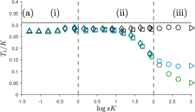
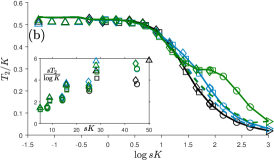
Figure S4: Mean extinction and absorption times $T_{1}$ and $T_{2}$, and mean fixation time $T_{F}$ in the constant-$K$ BDCLV for $K\in\{1000~{}(\rhd),450~{}(\circ),250~{}(\diamond),90~{}(\square),50~{}(\triangle)\}$ and the same values of $s$ as in Figs. 3 and 4: (a) $T_{1}/K$ vs. $sK$; showing $T_{1}={\cal O}(K)$ when $K\gg 1$ and $T_{1}\approx 0.31K$ (dotted line) when $r_{i}=r$ and under weak selection ($sK\lesssim 10$) when $\vec{x}_{c}\neq\vec{x}^{*}$ (unequal $r_{i}$’s), see text. (b) $T_{2}/K$ vs. $sK$; solid and dashed lines show the respective predictions of $T_{2}|_{K}=\sum_{i}\phi_{i,i+1}T_{2}^{(i,i+1)}|_{K}$ and (S29), see text. Inset: $sT_{2}/\log{K}={\cal O}(1)$ when $s\ll 1$ and $sK\gg 1$, see text. (c) $T_{F}/K$ vs. $sK$ showing that $T_{F}={\cal O}(K)$ across all regimes with subleading prefactors in regime (iii) shorter than in (i) and (ii). In all panels: symbols are from stochastic simulations, $\vec{x}_{0}=\vec{x}_{c}$, $\epsilon=0$ and $r_{1}=1/11$ (green), $1$ (black), $3/5$ (blue) and $r_{2}=r_{3}=1$.

E.1.1 Stage 1: Mean extinction time $T_{1}$ in the constant-$K$ BDCLV

The mean extinction time $T_{1}$ is the average time for one of the species to go extinct at the end of Stage 1. As explained in B, with the results obtained for the cCLV, we find $T_{1}\simeq T_{1}^{{\rm cCLV}}/2\approx 0.3K$ when $s\ll 1$ (regimes (i,ii)) and for arbitrary $s$ when all $r_{i}=1/3$, see Fig. S4 (a). Deviations from $T_{1}\approx 0.3K$, and a weak dependence on $s$ and on the $r_{i}$’s, are found near the boundary of regimes (ii)-(iii) and in regime (iii), where $T_{1}\simeq\beta_{c}(s,\vec{r})K$, where $\beta_{c}$ is a decreasing function of $s$ when the $r_{i}$’s are unequal, see Fig. S4 (a).

E.1.2 Stage 2: Mean absorption time $T_{2}$ in the constant-$K$ BDCLV

The stage 2 mean absorption time $T_{2}$ is given by

$$T_{2}=\sum_{i=1}^{3}\phi_{i,i+1}T_{2}^{(i,i+1)},$$ (S28)

where the mean absorption time along the edge $(i,i+1)$ of $S_{3}$, denoted by $T_{2}^{(i,i+1)}$, is weighted by the probability $\phi_{i,i+1}$ that Stage 1 ends on that edge.

The expression of $T_{2}^{(i,i+1)}$ is obtained from the mean fixation time of the MCLV with $N=K$, here denoted by $T_{2}^{(i,i+1)}|_{K}$ with $T_{2}^{(i,i+1)}\simeq T_{2}^{(i,i+1)}|_{K}$, see C. For a given initial fraction $\hat{x}_{i}$ of $i$’s at the start of Stage 2 is $(\hat{x}_{i})$, $T_{2}^{(i,i+1)}(\hat{x}_{i})|_{K}$ when $s\ll 1$ is obtained by solving ${\cal G}_{(i,i+1)}|_{K}(\hat{x}_{i})~{}T_{2}^{(i,i+1)}(\hat{x}_{i})|_{K}=-1$, with $T_{2}^{(i,i+1)}|_{K}(0)=T_{2}^{(i,i+1)}|_{K}(1)=0$, see (S24). Since the exact population composition along the edge $(i,i+1)$ at the inception of Stage 2 is given by $P_{(i,i+1)}(\hat{x}_{i})$, we have:

$$T_{2}\simeq\sum_{i=1}^{3}\phi_{i,i+1}T_{2}^{(i,i+1)}|_{K}=\sum_{i=1}^{3}\phi_{i,i+1}\int_{0}^{1}P_{(i,i+1)}(\hat{x}_{i})~{}T_{2}^{(i,i+1)}(\hat{x}_{i})|_{K}~{}d\hat{x}_{i}.,$$

with $T_{2}^{(i,i+1)}|_{K}\equiv\int_{0}^{1}P_{(i,i+1)}(\hat{x}_{i})~{}T_{2}^{(i,i+1)}(\hat{x}_{i})|_{K}~{}d\hat{x}_{i}$. A simpler expression for $T_{2}$ is obtained when $s\ll 1$ and $sK={\cal O}(10)$ upon substituting $\phi_{i,i+1}\approx 1/3$ and $P_{(i,i+1)}\approx 1$ in (E.1.2):

$$T_{2}\simeq\frac{1}{3}\sum_{i=1}^{3}\int_{0}^{1}T_{2}^{(i,i+1)}(\hat{x}_{i})|_{K}~{}d\hat{x}_{i}.$$ (S29)

While the expression of $T_{2}^{(i,i+1)}(\hat{x}_{i})$ is not particularly illuminating, its asymptotic behavior is simple and allows us to determine the behavior of $T_{2}$: In the weak-selection regime (ii) where $s\ll 1$ and $sK={\cal O}(10)$, we obtain the classical result $T_{2}^{(i,i+1)}|_{K}={\cal O}((\log{K})/s)$ according to which $T_{2}$ scales as $1/s$ with a subleading prefactor $\sim\log{K}$ [3, 79], which is confirmed by the results of Fig. S4 (c).

On the other hand, since the mean fixation time in the neutral Moran model scales linearly with the population size [3, 2, 79], we readily find $T_{2}={\cal O}(K)$ in the quasi-neutral regime (i). The mean fixation time in the Moran model with strong selection favoring species $i$ against $i+1$ scales logarithmically with the population size [80], from which we infer that $T_{2}={\cal O}(\log{K})$ in regime (iii).

Putting the asymptotic behaviors of $T_{1}$ and $T_{2}$ together, we find that to leading order in $N\simeq K\gg 1$ the overall mean fixation time $T_{F}=T_{1}+T_{2}={\cal O}(K)$ scales linearly with the population size across the regimes (i)-(iii), with different subleading prefactors in each regime. We also notice that in regime (iii) $T_{1}\gg T_{2}$: The extinction of a second species (Stage 2) occurs much faster than the death of a first species in Stage 1, see Fig. 1(a). In regime (i) $T_{1}/T_{2}={\cal O}(1)$ and $T_{1}/T_{2}={\cal O}(sK/\log{K})$ in regime (ii), see Fig. 1(b).

E.2 Mean extinction, absorption and fixation times in the switching-$K$ BDCLV

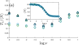
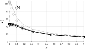
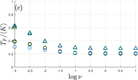
Figure S5: (a) $T_{1}/\langle N\rangle$ vs. $\nu$ for $r_{1}=1/11\text{(green)},1/3\text{(black)},3/5\text{(blue)}$ and $r_{2}=r_{3}=(1-r_{1})/2$, with $s=10^{-1/2}$ (circles) and $s=10^{-3/2}$ (triangles). In agreement with (S30), $T_{1}/\langle N\rangle=\beta_{s}={\cal O}(1)$ and slowly varies with $\nu$ and $s$. Inset: $\langle N\rangle$ vs $\nu$; solid lines are from the average over the marginal probability density (22) of the process defined by (S8), and symbols are from stochastic simulations with $s=10^{-1/2}$ (circles) and $s=10^{-3/2}$ (triangles), showing $\langle N\rangle={\cal O}(\langle K\rangle)$, see text. (b) $T_{2}$ vs. $s$ for $\nu=10^{-3}$ (circles, light dotted gray), $10^{-1}$ (diamonds, dashed gray), $10$ (squares, solid black) and $\vec{r}=(1/3,1/3,1/3)$. Symbols are from stochastic simulations and lines are from (S31). $T_{2}$ scales as $1/s$ with subleading prefactor $\sim\log{\langle K\rangle}$ when $s\ll 1$ and $s\langle K\rangle={\cal O}(10)$, see text. (c) Same as in (a) but for the overall mean fixation time: $T_{F}/\langle K\rangle$ vs. $\nu$ with $s=10^{-1/2}$ (circles) and $s=10^{-3/2}$ (triangles), showing $T_{F}={\cal O}(\langle K\rangle)$ over a broad range of values $\nu$, see text. In all panels: $\langle K\rangle=250,\gamma=0.8$ $(K_{-}=50,K_{+}=450)$ and $\vec{x}_{0}=\vec{x}_{c}$; $\epsilon=0$.

We study the effect of random switching on the mean extinction and absorption times, $T_{1}$ and $T_{2}$ characterizing Stages 1 and 2, respectively. This allows us to show that the mean fixation time $T_{F}=T_{1}+T_{2}={\cal O}(\langle N\rangle)={\cal O}(\langle K\rangle)$ scales linearly with the average population size, and to compute the average number of switches occurring in Stages 1 and 2.

E.2.1 Stage 1: Mean extinction time in the switching-$K$ BDCLV

Guided by the results of the constant-$K$ BDCLV, where $T_{1}$ scales linearly with $N\approx K$ to leading order in $\langle K\rangle\gg 1$, we expect

$$T_{1}=\beta_{s}\langle N\rangle\quad\text{with}\quad\beta_{s}=\beta_{s}(s,\vec{r},\nu),$$ (S30)

where $\langle N\rangle={\cal O}(\langle K\rangle)$ is the long-time average population size that is in principle obtained by averaging $N$ over the $N$-QSD. In the inset of Fig. S5, this quantity is accurately computed in the realm of the PDMP approximation as $\langle N\rangle=\int_{K_{-}}^{K_{+}}Np_{\nu}^{*}(N)dN$, see the inset of Fig. S5 (a), and is shown to be independent of $s$ and a decreasing function of $\nu$. For fast/slow switching, we have $\langle N\rangle=(1-\gamma^{2})\langle K\rangle$ when $\nu\to\infty$ and $\langle N\rangle=\langle K\rangle$ when $\nu\to 0$ [56, 57]. Comparison with simulation results of Fig. S5 confirm that $T_{1}/\langle N\rangle=\beta_{s}={\cal O}(1)$ is a slowly varying function of $\nu$ and a weakly decreasing function of $s$. Since $\langle N\rangle={\cal O}(\langle K\rangle)$ when $\gamma={\cal O}(1)$, we obtain $T_{1}={\cal O}(\langle N\rangle)={\cal O}(\langle K\rangle)$ to leading order in $\langle K\rangle$.

E.2.2 Stage 2 mean absorption time and overall mean fixation time in the switching-$K$ BDCLV

Proceeding as in Sec. 5.1.2, the Stage 2 mean absorption time is given by $T_{2}=\sum_{i=1}^{3}\phi_{i,i+1}T_{2}^{(i,i+1)}$. In the realm of the PDMP approximation, when $s\ll 1$ and $s\langle K\rangle\gg 1$, $T_{2}^{(i,i+1)}$ is obtained by averaging the constant-$\langle K\rangle$ mean absorption time $T_{2}^{(i,i+1)}|_{\langle K\rangle}$ along the edge $(i,i+1)$ over the probability density function (22)  [56, 57]:

$$T_{2}^{(i,i+1)}\simeq\int_{0}^{1}\int_{K_{-}}^{K_{+}}P_{(i,i+1)}(\hat{x}_{i})~{}T_{2}^{(i,i+1)}(\hat{x}_{i})|_{\langle K\rangle}~{}p_{\nu/\alpha_{i}}^{*}(N)~{}d\hat{x}_{i}~{}dN.$$

As in Sec. 4.1.2, the switching rate is rescaled $\nu\to\nu/\alpha_{i}$ due to the average number ${\cal O}(\nu/\alpha_{i})$ of switches occurring in Stage 2 along the edge $(i,i+1)$ when $s\ll 1$ and $s\langle K\rangle\gg 1$ [56, 57]. The above equation can be simplified using $\phi_{i,i+1}\approx 1/3$ and $P_{(i,i+1)}(\hat{x}_{i})\approx 1$ when $s\ll 1$ and $s\langle K\rangle\lesssim 10$ (D):

$$T_{2}\approx\frac{1}{3}\sum_{i=1}^{3}T_{2}^{(i,i+1)}\simeq\frac{1}{3}\sum_{i=1}^{3}\int_{K_{-}}^{K_{+}}T_{2}^{(i,i+1)}(\hat{x}_{i})|_{\langle K\rangle}~{}p_{\nu/\alpha_{i}}^{*}(N)~{}dN,$$ (S31)

where $T_{2}^{(i,i+1)}\sim T_{2}^{(i,i+1)}|_{\langle K\rangle}(\hat{x}_{i})$ which scales as $1/\alpha_{i}$ with a prefactor $\sim\log{\langle K\rangle}$ and a weak dependence on $\nu$ when $s\ll 1$ and $s\langle K\rangle\gg 1$ [56]. This yields $T_{2}^{(i,i+1)}={\cal O}((\log{\langle K\rangle})/s)$ in regime (ii): In agreement with the results of Fig. S5 (b), $T_{2}={\cal O}(1/s)$ with a subleading prefactor $\sim\log{\langle K\rangle}$ when $s\ll 1$ and $s\langle K\rangle\lesssim 10$. As in the constant-$K$ BDCLV, the quasi-neutral regime (i), where $s\langle K\rangle\ll 1$, $T_{2}={\cal O}(\langle K\rangle)$, whereas under strong selection, $s\langle K\rangle\gg 1$, $T_{2}={\cal O}(\log{\langle K\rangle})$, see Fig. S5 (b).
Putting together the results for $T_{1}$ and $T_{2}$, we obtain the overall mean fixation time $T_{F}=T_{1}+T_{2}\sim\langle N\rangle$. Since $\langle N\rangle={\cal O}(\langle K\rangle)$, we have $T_{F}={\cal O}(\langle K\rangle)$ which, with subleading prefactors that vary slowly with $\nu$ and $s$, as illustrated by Fig. S5(c).

E.3 Average number of switches in Stages 1 and 2 of the switching-$K$ BDCLV

Since the average duration of Stage 1 in the the switching-$K$ BDCLV is $T_{1}=\beta_{s}\langle N\rangle={\cal O}(\langle K\rangle)$, see Eq. (S30), the average number of switches occurring prior one of the species die out scales as ${\cal O}(\nu\langle K\rangle)$ as shown in Fig. S6 (a), i.e. the average number of switches increases as $\nu\langle K\rangle$, with a prefactor that depends on $s$ via $\beta_{s}$ which is a weakly decreasing function of $s$ (i.e. the number of switches is greater for smaller values of $s$). Hence, for any non-vanishingly small switching rate $\nu\gg 1/\langle K\rangle$ and $\langle K\rangle\gg 1$, a large number of switches occur during Stage 1 prior to the extinction of the first species and the DMN self averages, see Sec. 4.1.1.

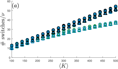
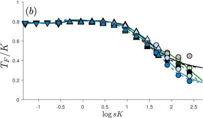
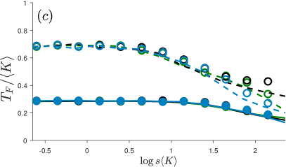
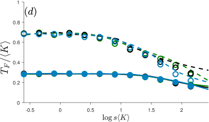
Figure S6: (a) Average number of switches in Stage 1 of the BDCLV for $\nu=0.1$ (circles), $1$ (triangles), $10$ (squares). Selection intensity is $s=10^{-3/2}$ (filled symbols) and $s=10^{-1/2}$ (open symbols). Data for (average number of switches in Stage 1)/$\nu$ vs $\langle K\rangle$ and different values of $\nu$ and $\vec{r}$ essentially collapse onto a curve (almost a line). (b) Rescaled mean fixation time $T_{F}/K$ vs. $sK$ in the close-to-zero-sum game ($|\epsilon|\ll 1$) and constant $K$ for values of $s\in(10^{-3},1)$ and $K=450$ (circles), $90$ (upward triangles), $50$ (downward triangles). Symbols are from stochastic simulations for $\epsilon=-0.2$ (light) and $\epsilon=0.2$ (dark). Lines are from the constant-$K$ BDCLV obtained with the same carrying capacity but a rescaled selection intensity $s(1+\epsilon/2)$. (c) $T_{F}/\langle K\rangle$ vs. $s\langle K\rangle$ when $K$ switches between $K_{-}=50$ and $K_{+}=450$ with $s\in(10^{-3},10^{-1/4})$, and $\nu=10$ (closed symbols) and $\nu=0.001$ (open symbols). Symbols are from stochastic simulations obtained for $\epsilon=-0.2$; solid ($\nu=10$) and dashed ($\nu=0.001$) lines are from the switching-$K$ BDCLV obtained with the same $K(t)$ but selection intensity $s(1+\epsilon/2)=0.9s$. (d) Same as in panel (c) with $\epsilon>0$: Symbols are stochastic simulation results for $\epsilon=0.2$; solid ($\nu=10$) and dashed ($\nu=0.001$) lines are results from the BDCLV with same switching carrying capacity and selection intensity $s\to s(1+\epsilon/2)=1.1s$. In all panels: $\vec{r}=(1,1,1)/3$ (black), $\vec{r}=(1,5,5)/11$ (green), $\vec{r}=(3,2,2)/5$ (blue); $\vec{r}=\vec{r}^{(1)}$ and $\vec{x}_{0}=\vec{x}_{c}$. In panels (a) and (b): dark symbols and solid lines are for $\epsilon=0.2$, light symbols and dashed lines are for $\epsilon=-0.2$.

In Refs. [56, 57], it has been shown that that under weak selection the population experiences, on average, ${\cal O}(\nu/\alpha_{i})$ switches during the two-species competition characterizing the stage 2 dynamics along the edge $(i,i+1)$. This supports the rescaling $\nu\to\nu/\alpha_{i}$ in formula (27) which has been found to be actually valid when the selection intensity $s$ is neither vanishingly small nor too large [57].

E.4 Mean fixation time of a close-to-zero-sum rock-paper-scissors game in fluctuating populations

The mean fixation time of the close-to-zero-sum rock-paper-scissors game ($|\epsilon|\ll 1$) under weak selection can be obtained with a similar argument usd in Sec. 5 for the fixation probabilities. In fact, the mean absorption time $T_{2}$ and the mean fixation time $T_{F}=T_{1}+T_{2}$ ($T_{1}$ varies little with $s$ in regime (ii), see Fig. S4 (a)) under weak selection can be obtained from their values in the BDCLV with a rescaled selection intensity $s\to s(1+(\epsilon/2))$, as shown in Fig. S6 (b)-(d). This is valid both for the case of a constant $K$, see Fig. S6 (b), and a randomly switching carrying capacity, see Fig. S6 (c,d). This confirms that the effect of $0<\epsilon\ll 1$ on the fixation properties simply boils down to increasing the selection intensity by a factor $1+(\epsilon/2)$ with respect to the BDCLV when $sK$ and $s\langle K\rangle$ are in regimes (i) and (ii). When $sK\gg 1$ and $s\langle K\rangle\gg 1$ (regime (iii)), the above argument breaks down and rescaling the selection intensity of the BDCLV’s mean fixation time is no longer a good approximation: Under strong selection, the actual $T_{F}$ is systematically overestimated and underestimated by the $s\to s(1+(\epsilon/2))$ rescaling when $\epsilon>0$ and $\epsilon<0$. Deviations from the rescaled BDCLV results are particularly pronounced under strong selection in the case $\epsilon<0$ and $\vec{x}_{c}=\vec{x}^{*}$ (with $r_{i}=1/3$).

References

- [1] E. Pennisi, Science, 309, 90 (2005).
- [2] J. F. Crow and M. Kimura, An Introduction to Population Genetics Theory (Blackburn Press, New Jersey, 2009).
- [3] W. J. Ewens, Mathematical Population Genetics (Springer, New York, 2004).
- [4] M. Frean; E. D. Abraham, Proc. R. Soc. Lond. B 268, 1323 (2001).
- [5] M. Ifti and B. Bergensen, Eur. Phys. J. E, 10, 241 (2003).
- [6] M. Berr, T. Reichenbach, M. Schottenloher and E. Frey, Phys. Rev. Lett. 102, 048102 (2009).
- [7] E. Frey, Physica A, 389, 4265 (2010).
- [8] T. Reichenbach, M. Mobilia and E. Frey, Nature (London) 448, 1046 (2007).
- [9] A. Szolnoki, M. Mobilia, L.-L. Jiang, B. Szczesny, A. M. Rucklidge, and M. Perc, J. R. Soc. Interface 11, 20140735 (2014).
- [10] B. Kerr, M. A. Riley, M. W. Feldman, and B. J. M. Bohannan, Nature (London) 418, 171 (2002).
- [11] J. B. C. Jackson and L. Buss, Proc. Nat. Acad. Sci. USA, 72, 5160 (1975).
- [12] B. Sinervo and C. M. Lively, Nature (London) 380, 240 (1996).
- [13] J. Maynard Smith, Evolution and the Theory of Games (Cambridge University Press, Cambridge , U.K.).
- [14] J. Hofbauer and K. Sigmund, K., Evolutionary games and population dynamics (Cambridge University Press, U.K., 1998).
- [15] R. M. Nowak, Evolutionary Dynamics (Belknap Press, Cambridge, USA, 2006).
- [16] G. Szabó and G. Fáth, Phys. Rep. 446 97 (2007)
- [17] M. Broom and J. Rychtář, Game-Theoretical Models in Biology (CRC Press, Boca Raton, USA, 2013).
- [18] U. Dobramysl, M. Mobilia, M. Pleimling, and U. C. Täuber, J. Phys. A: Math. Theor. 51, 063001 (2018)
- [19] T. Reichenbach, M. Mobilia and E.Frey, Phys. Rev. E 74, 051907 (2006).
- [20] R. M. May and W. J. Leonard, SIAM J. Appl. Math. 29, 243 (1975).
- [21] T. Reichenbach, M. Mobilia, and E. Frey, Banach Centre Publications 80, 259 (2008).
- [22] K. I. Tainaka, Phys. Rev. Lett. 63, 2688 (1989).
- [23] K. I. Tainaka, Phys. Lett. A 176, 303 (1993).
- [24] K. I. Tainaka, Phys. Rev. E 50, 3401 (1994).
- [25] Q. He, M. Mobilia, and U. C. Täuber, Phys. Rev. E 82, 051909 (2010).
- [26] X. Ni, W. X. Wang, Y. C. Lai, and C. Grebogi, Phys. Rev. E 82, 066211 (2010).
- [27] S. Venkat and M. Pleimling, Phys. Rev. E 81, 021917 (2010).
- [28] A. Dobrinevski and E. Frey, Phys. Rev. E 85, 051903 (2012).
- [29] J. Knebel, T. Krüger, M. F. Weber, and E. Frey Phys. Rev. Lett. 110 168106 (2013).
- [30] N. Mitarai, I. Gunnarson, B. N. Pedersen, C. A. Rosiek, and K. Sneppen, Phys. Rev. E 93, 042408 (2016).
- [31] G. Szabó and A. Szolnoki, Phys. Rev. E 65, 036115 (2002).
- [32] M. Perc, A. Szolnoki, and G. Szabó, Phys. Rev. E 75, 052102 (2007).
- [33] R. West, M. Mobilia and A. M. Rucklidge, Phys. Rev. E 97, 022406 (2018).
- [34] C. A. Fux, J. W. Costerton, P. S. Stewart, and P. Stoodley, Trends Microbiol. 13, 34 (2005).
- [35] R. M. May, Stability and Complexity in Model Ecosystems (Princeton University Press, Princeton, New Jersey, 1974).
- [36] E. Kussell, R. Kishony, N. Q. Balaban, and S. Leibler, Genetics 169, 1807 (2005).
- [37] M. Acer, J. Mettetal, and A. van Oudenaarden, Nature Genetics 40, 471 (2008);
- [38] P. Visco, R. J. Allen, S. N. Majumdar, M. R. Evans, Biophys. J. 98, 1099 (2010).
- [39] U. Dobramysl, and U. C.Täuber, Phys. Rev. Lett. 110, 048105 (2013).
- [40] M. Assaf, E. Roberts, Z. Luthey-Schulten, and N. Goldenfeld, Phys. Rev. Lett. 111, 058102 (2013).
- [41] M. Assaf, M. Mobilia, and E. Roberts, Phys. Rev. Lett. 111, 011134 (2013).
- [42] P. Ashcroft, P. M. Altrock, and T. Galla, J. R. Soc. Interface 11, 20140663 (2014).
- [43] P. G. Hufton, Y. T. Lin, T. Galla, and A. J. McKane, Phys. Rev. E 93, 052119 (2016).
- [44] J. Hidalgo, S. Suweis, and A. Maritan, J. Theor. Biol. 413, 1 (2017).
- [45] B. Xue and S. Leibler, Phys. Rev. Lett. 119, 108103 (2017).
- [46] M. Danino and N. M. Shnerb, J. Theor. Biol. 441, 84 (2018).
- [47] P. G. Hufton, Y. T. Lin, and T. Galla, and A. J. McKane, Phys. Rev. E 99, 032122 (2019).
- [48] R. Levins, Evolution in Changing environments: some Theoretical Explorations (Princeton University Press, Princeton, New Jersey, 1968).
- [49] J. Roughgarden, Theory of Population Genetics and Evolutionary Ecology: An Introduction (Macmillan, New York, 1979).
- [50] J. S. Chuang, O. Rivoire, and S. Leibler S, Science 323, 272 (2009).
- [51] A. Melbinger, J. Cremer, and E. Frey, Phys. Rev. Lett. 105, 178101 (2010).
- [52] E. A. Yurtsev, H. Xiao Chao, M. S. Datta, T. Artemova, and J. Gore, Molecular Systems Biology 9, 683 (2013).
- [53] A. Sanchez and J. Gore, PLoS Biology 11, e1001547 (2013).
- [54] K. I. Harrington and A. Sanchez, Communicative & Integrative Biology 7, e28230:1-7.
- [55] A. Melbinger, J. Cremer, and E. Frey, J. R. Soc. Interface 12, 20150171 (2015).
- [56] K. Wienand, E. Frey, and M. Mobilia, Phys. Rev. Lett 119, 158301 (2017).
- [57] K. Wienand, E. Frey, and M. Mobilia, J. R. Soc. Interface 15, 20180343 (2018).
- [58] A. McAvoy, N. Fraiman, C. Hauert, J. Wakeley, and M. A. Nowak, Theor. Popul. Biol. 121, 72 (2018).
- [59] L. M. Wahl, P. J. Gerrish, and I. Saika-Voivod, Genetics 162, 961 (2002).
- [60] M. A. Brockhurst, A. Buckling, and A. Gardner, Curr. Biol. 17, 761 (2007).
- [61] Z. Patwas and L. M. Wahl, Evolution 64, 1166 (2009).
- [62] H. A. Lindsey, J. Gallie, S. Taylor, and B. Kerr, Nature (London) 494, 463 (2013).
- [63] W. Horsthemke and R. Lefever, Noise-Induced Transitions (Springer, Berlin, 2006).
- [64] I. Bena, Int. J. Mod. Phys. B 20, 2825 (2006).
- [65] K. Kitahara, W. Horsthemke, and R. Lefever, Phys. Lett. 70A, 377 (1979).
- [66] M. H. A. Davis, J. R. Stat. Soc. B 46, 353 (1984).
- [67] J.-C. Claussen and A. Traulsen, Phys. Rev. Lett. 100, 058104 (2008).
- [68] M. Mobilia, J. Theor. Biol. 264, 1 (2010).
- [69] T. Galla, J. Theor. Biol. 269, 46 (2011).
- [70] T. Reichenbach, M. Mobilia, and E. Frey, Phys. Rev. Lett. 99, 238105 (2007).
- [71] T. Reichenbach, M. Mobilia, and E. Frey, J. Theor. Biol. 254, 368 (2008).
- [72] Q. He, M. Mobilia, and U. C. Täuber, Eur. Phys. J. B 82, 97 (2011).
- [73] B. Szczesny, M. Mobilia and A. M. Rucklidge, EPL (Europhysics Letters) 102, 28012 (2013).
- [74] B. Szczesny, M. Mobilia and A. M. Rucklidge, Phys. Rev. E 90, 032704 (2014).
- [75] M. Mobilia, A. M. Rucklidge, and B. Szczesny, Games 7, 24 (2016).
- [76] Q. Yang, T. Rogers, and J. H. P. Dawes, J. Theor. Biol. 432, 157 (2017).
- [77] C. M. Postlethwaite and A. M. Rucklidge, EPL (Europhysics Letters) 117, 48006 (2017)
- [78] P. A. P. Moran, The statistical processes of evolutionary theory. (Clarendon, Oxford, 1962).
- [79] R. A. Blythe and A. J. McKane, J. Stat. Mech. P07018 (2007).
- [80] T. Antal and I. Scheuring, Bull. Math. Biol. 68, 1923 (2006).
- [81] C. Spalding, C. R. Doering, and G. R. Flierl, Phys. Rev. E 96, 042411 (2017).
- [82] C. Gardiner, Handbook of Stochastic Methods (Springer, New York, U.S.A., 2002).
- [83] N. G. Van Kampen, Stochastic Processes in Physics and Chemistry (Elsevier, Amsterdam, Netherland, 1992).
- [84] D. T. Gillespie, J. Comput. Phys. 22, 403 (1976).
- [85] Supplementary Material is electronically available at the following URL: https://doi.org/10.6084/m9.figshare.8858273.v1.
Appendix: Supplementary Material for