Spectrum of the fully-heavy tetraquark state $QQ\bar{Q}^{\prime}\bar{Q}^{\prime}$

Abstract

In this work, we systematically calculate the mass spectra of the $S$-wave fully heavy tetraquark states $bb\bar{b}\bar{b}$, $cc\bar{c}\bar{c}$, and $bb\bar{c}\bar{c}$ in two nonrelativistic quark models. A tetraquark state may be an admixture of a $6_{c}-\bar{6}_{c}$ state and a $\bar{3}_{c}-3_{c}$ one, where $6_{c}-\bar{6}_{c}$($\bar{3}_{c}-3_{c}$) denotes the color configuration with a $6_{c}$ ($\bar{3}_{c}$) diquark and a $\bar{6}_{c}$ ($3_{c}$) antidiquark. For the tetraquark states $bb\bar{b}\bar{b}$ and $cc\bar{c}\bar{c}$ with $J^{PC}={0^{++}}$, the $6_{c}-\bar{6}_{c}$ state is lower than the $\bar{3}_{c}-3_{c}$ one in both the two quark models, while the order of the $bb\bar{c}\bar{c}$ states depend on models. The $6_{c}-\bar{6}_{c}$ and $\bar{3}_{c}-3_{c}$ mixing effects are induced by the hyperfine interactions between the diquark and antidiquark, while the contributions from the one-gluon-exchange (OGE) Coulomb or the linear confinement potentials vanish for the $QQ\bar{Q}^{\prime}\bar{Q}^{\prime}$ system. With the couple-channel effects, we obtain the similar mass spectra. The numerical results show that the ground $QQ\bar{Q}^{\prime}\bar{Q}^{\prime}$ ($Q=b,c$ and $Q^{\prime}=b,c$) tetraquark states are located above the corresponding scattering states, which indicates that there may not exist a bound state in the scheme of the two quark models.

I introduction

Since 2003, numerous exotic structures have been observed in experiments Choi:2007wga ; Aaij:2014jqa ; Chilikin:2013tch ; Chilikin:2014bkk ; Ablikim:2013xfr ; Ablikim:2013wzq ; Ablikim:2013mio ; Belle:2011aa ; Adachi:2012cx ; Aaij:2015tga ; Aaij:2018bla , amongst which many states cannot be accommodated into the traditional quark model. In the literature, there are many possible explanations. The most prominent ones are the molecules (loosely bound states of two hadrons), the tetraquarks (compact bound states), and the hybrids (composed of gluons and quarks), etc. For a recent review, see Refs. Chen:2016qju ; Guo:2017jvc ; Esposito:2016noz ; Ali:2017jda ; Liu:2019zoy .

A fully heavy tetraquark state is a topic of great interest. The interactions between the heavy quarks may be dominated by the short-range one-gluon-exchange (OGE) potential rather than the long-range potentials. Thus, they are good candidates of the compact tetraquark states. Unlike a meson or a baryon where the color configuration of the quarks is unique, i.e. $q_{i}\bar{q}_{j}\delta_{ij}$ or $\epsilon_{ijk}q_{i}q_{j}q_{k}$, the color structure for the tetraquark is much richer. For the tetraquark states, the four quarks can neutralize the color in two ways, $6_{c}\otimes\bar{6}_{c}=1_{c}$ and $\bar{3}_{c}\otimes 3_{c}=1_{c}$. In this work, we label the two color configurations $|(QQ)_{6_{c}}{\bar{Q}\bar{Q}}_{\bar{6}_{c}}\rangle$ and $|(QQ)_{\bar{3}_{c}}{\bar{Q}\bar{Q}}_{3_{c}}\rangle$ as $6_{c}-\bar{6}_{c}$ and $\bar{3}_{c}-3_{c}$, respectively. In Refs. Maiani:2004vq ; Ali:2011ug ; Eichten:2017ffp , the authors investigate the tetraquark states in the $\bar{3}_{c}-3_{c}$ configuration. In Refs. Chen:2016oma ; Maiani:2019cwl , the authors pointed out that the $6_{c}-\bar{6}_{c}$ configuration is also very important to form the tetraquark states. The fully heavy tetraquark state is a golden system to investigate the inner color configuration of the multiquark states. For the above reasons, the fully heavy tetraquark states have inspired both the experimental and theoretical attention.

Recently, the CMS collaboration observed the $\Upsilon(1S)$ pair production and indicated a $bb\bar{b}\bar{b}$ signal around $18.4$ GeV with a global significance of $3.6\sigma$ Khachatryan:2016ydm ; S. Durgut . Later, the LHCb searched the invariant mass distribution of $\Upsilon(1s)\mu^{+}\mu^{-}$ and did not observe the tetraquark state $X_{bb\bar{b}\bar{b}}$ Aaij:2018zrb . The tension between CMS and LHCb data requires more experimental and theoretical studies of the fully-beauty tetraquarks.

The mass spectroscopy has been a major platform to probe the dynamics of the tetraquarks. Since 1975, there have been many theoretical works about the mass spectroscopy of the fully heavy quark states Iwasaki:1975pv ; Chao:1980dv ; Ader:1981db ; Zouzou:1986qh ; Heller:1986bt ; SilvestreBrac:1992mv ; SilvestreBrac:1993ry . The existence of the fully heavy quark states is still controversial. Recent interests have followed the experimental developments in the past several years. The mass spectra have been calculated in different schemes, for instance, a diffusion Monte Carlo method Bai:2016int , the non-relativistic effective field theory (NREFT) Anwar:2017toa , the QCD sum rules Wang:2017jtz ; Wang:2018poa ; Chen:2018cqz , covariant Bethe-Salpeter equations Heupel:2012ua , various quark models Lloyd:2003yc ; Debastiani:2017msn ; Barnea:2006sd , and other phenomenological models Berezhnoy:2011xy ; Berezhnoy:2011xn ; Karliner:2016zzc ; Esposito:2018cwh ; Karliner:2017qhf . The lowest $bb\bar{b}\bar{b}$ and $cc\bar{c}\bar{c}$ states are estimated to be in the mass range $18-20$ GeV and $5-7$ GeV, respectively. In contrast, the authors of Ref. Wu:2016vtq investigated the mass spectra of the $QQ\bar{Q}\bar{Q}$ states in the Chromomagnetic interaction (CMI) model and concluded that no stable $QQ\bar{Q}\bar{Q}$ states exist. Later, several other approaches, such as the nonrelativistic chiral quark model Chen:2019dvd ; Liu:2019zuc , the lattice QCD Hughes:2017xie and other models Richard:2017vry ; Czarnecki:2017vco also do not support the existence of the bound $QQ\bar{Q}\bar{Q}$ states.

To investigate the existence of the full heavy tetraquark states, we systematically calculate the mass spectra of the $bb\bar{b}\bar{b}$, $cc\bar{c}\bar{c}$ and $bb\bar{c}\bar{c}~{}(cc\bar{b}\bar{b})$ in two non-relativistic quark models. In general, a tetraquark state should be an admixture of the two color configurations, $6_{c}-\bar{6}_{c}$ and $\bar{3}_{c}-3_{c}$. In this work, with the couple-channel effects, we perform the dynamical calculation of the mass spectra of the tetraquark states and investigate the inner structures of the ground states.

We organize the paper as follows. In Sec. II, we introduce the formalism to calculate their mass spectra, including two non-relativistic quark models, the construction of the wave functions, and the analytical expressions of the Hamiltonian matrix elements. In Sec. III, we present the numerical results and discuss the couple-channel effects between the $\bar{3}_{c}-3_{c}$ and $6_{c}-\bar{6}_{c}$ configurations. In Sec. IV, we compare our results with those in other models and give a brief summary.

II formalism

II.1 Hamiltonian

The nonrelativistic Hamiltonian of a $Q_{1}Q_{2}\bar{Q}_{3}\bar{Q}_{4}$ tetraquark state reads

$$H = \sum_{i=1}^{4}\frac{p_{j}^{2}}{2m_{j}}+\sum_{i<j}V_{ij}+\sum_{i}m_{i}$$ (1)

$$= \frac{p^{2}}{2u}+V_{I}+h_{12}+h_{34}$$

with

$$V_{I}=V_{13}+V_{14}+V_{23}+V_{24},$$ (2)

$$h_{ij}=\frac{p_{ij}^{2}}{2u_{ij}}+V_{ij}+m_{i}+m_{j},$$ (3)

$$\mathbf{p}_{ij}=\frac{m_{i}\mathbf{p}_{j}-m_{j}\mathbf{p}_{i}}{m_{i}+m_{j}},\,\,\ u_{ij}=\frac{m_{i}m_{j}}{m_{i}+m_{j}},$$ (4)

$$m_{ij}=m_{i}+m_{j},\,\,\ u={{m_{12}m_{34}}\over{m_{12}+m_{34}}},$$ (5)

$$\mathbf{P}_{ij}=\mathbf{p}_{i}+\mathbf{p}_{j},\,\,\mathbf{p}=\frac{m_{12}\mathbf{P}_{34}-m_{13}\mathbf{P}_{24}}{m_{12}+m_{34}}.$$ (6)

where $\mathbf{p}_{i}$ and $m_{i}$ are the momentum and mass of the $i$th quark. The kinematic energy of the center-of-mass system has been excluded by the constraint $\sum^{4}_{i=1}\mathbf{p}_{i}=0$. $V_{ij}$ is the potential between the $i$th and $j$th quarks. The $u_{ij}$, $m_{ij}$, $\mathbf{p}_{ij}$, and $\mathbf{P}_{ij}$ are the reduced mass, total mass, relative momentum, and total momentum of the $(ij)$ pair of quarks, respectively. The $u$ and $\mathbf{p}$ are the reduced mass and relative momentum between the $(12)$ and $(34)$ quark pairs. $h_{12}$, $h_{34}$ and $V_{I}$ represent the $(12)$ quark pair inner interaction, $(34)$ quark pair interaction and interaction between the two pairs.

Since the heavy quark mass is large, the relativistic effect is less important. We use a nonrelativistic quark model to describe the interaction between two heavy quarks. The quark model proposed in Ref. Wong:2001td contains one gluon exchange (OGE) plus a phenomenological linear confinement interaction and the $V_{ij}$ reads

$$V_{ij}(r_{ij})=\frac{\mathbf{\lambda}_{i}}{2}\frac{\mathbf{\lambda}_{j}}{2}\left(V_{\text{coul}}+V_{\text{conf}}+V_{\text{hyp}}+V_{\text{cons}}\right)$$

$$=\frac{\lambda_{i}}{2}\frac{\lambda_{j}}{2}\left(\frac{\alpha_{s}}{r_{ij}}-\frac{3b}{4}r_{ij}-\frac{8\pi\alpha_{s}}{3m_{i}m_{j}}\mathbf{s}_{i}\cdot\mathbf{s}_{j}e^{-\tau^{2}r^{2}}\frac{\tau^{3}}{\pi^{3/2}}+V_{\text{cons}}\right),$$

where $\lambda$ is the color matrix (replaced by $-\lambda^{*}$ for an antiquark). $\mathbf{s}_{i}$ is the spin operator of the $i$th quark. $r_{ij}$ is the relative position of the $i$th and $j$th quarks. $V_{\text{coul}}$, $V_{\text{conf}}$, and $V_{\text{hyp}}$ represent the OGE color Coulomb, the linear confinement, and the hyperfine interactions, respectively. The OGE interaction leads to a contact hyperfine effect and an infinite hyperfine splitting. In Eq. (II.1), the smearing effect has been considered in $V_{\text{hyp}}$.

The $\alpha_{s}$ is the running coupling constant in the perturbative QCD,

$$\alpha_{s}(Q^{2}) = \frac{12\pi}{(33-2N_{f})\ln(A+Q^{2}/B^{2})}.$$ (8)

In this work, we take the square of the invariant mass of the interacting quarks as the scale $Q^{2}$. The values of the parameters are listed in Table 1. They are determined by fitting the mass spectra of the mesons as listed in Table 2.

Table 1: The values of parameters in quark model I Wong:2001td and model II SilvestreBrac:1996bg .

Model I			$m_{c}$[GeV]	$m_{b}$[GeV]	$b[\text{GeV}^{2}]$	$\tau$[GeV]	$V_{\text{cons}}$[GeV]	$A$	$B$[GeV]
			$1.776$	$5.102$	$0.18$	$0.897$	$0.62$	$10$	$0.31$
Model II	$p$	$r_{c}$	$m_{c}$[GeV]	$m_{b}$[GeV]	$\kappa$	$\kappa^{\prime}$	$\lambda[\text{GeV}^{2}]$	$\Lambda$[GeV]	$A[\text{GeV}^{B-1}]$	$B$
	$1$	$0$	$1.836$	$5\text{.}227$	$0.5069$	$1.8609$	$0.1653$	$0.8321$	$1.6553$	$0.2204$

Table 2: The mass spectra of the heavy quarkonia in units of MeV. The $M_{\text{ex}}$, $M^{I}_{th}$, and $M^{II}_{th}$ refer to the mass spectra of mesons from experiments Tanabashi:2018oca , in model I Wong:2001td , and in model II SilvestreBrac:1996bg , respectively.

	$M_{\text{ex}}$	$M_{th}^{I}$	$M_{th}^{II}$		$M_{\text{ex}}$	$M_{th}^{I}$	$M_{th}^{II}$
$B_{c}$	$6274.9$	$6319.4$	$6293.5$
$\eta_{c}$	$2983.9$	$3056.5$	$3006.6$	$\eta_{b}$	$9399.0$	$9497.8$	$9427.9$
$\eta_{c}(2S)$	$3637.6$	$3637.6$	$3621.2$	$\Upsilon(1S)$	$9460.30$	$9503.6$	$9470.4$
$J/\psi$	$3096.9$	$3085.1$	$3102.1$	$\Upsilon(2S)$	$10023.26$	$9949.7$	$10017.8$
$\psi(2S)$	$3686.1$	$3652.4$	$3657.8$	$\Upsilon(3S)$	$10355.2$	$10389.8$	$10440.6$

To investigate the model dependence of the mass spectrum, we also consider another nonrelativistic quark model proposed in Ref. SilvestreBrac:1996bg . The potential reads

$$V_{ij}(r_{ij})=-\frac{3}{16}\sum_{i<j}\lambda_{i}\lambda_{j}\Big{(}-\frac{\kappa(1-\text{exp}(-r_{ij}/r_{c}))}{r_{ij}}+\lambda r_{ij}^{p}$$

$$-\Lambda+\frac{8\pi}{3m_{i}m_{j}}\kappa^{\prime}(1-\text{exp}(-r_{ij}/r_{c}))\frac{\text{exp}(-r_{ij}^{2}/r_{0}^{2})}{\pi^{3/2}r_{0}^{3}}\mathbf{s}_{i}\cdot\mathbf{s}_{j}\Big{)},$$

where $r_{0}=A(\frac{2m_{i}m_{j}}{m_{i}+m_{j}})^{-B}$ is related to the reduced mass of the two quarks $(ij)$. In this model, all the mass information is included in the hyperfine potential, which is expected to play a more important role than that in Model I. The parameters of the potentials are listed in Table 1. With these parameters, we calculate the mass spectra of the mesons and list them in Table 2.

In this work, we concentrate on the $S$-wave tetraquark states and do not include the tensor and spin-orbital interactions in the two quark models. In Table 2, we notice that both models are able to reproduce the mass spectra of the heavy quarkonia. In the following, we will extend the two quark models to study the fully heavy tetraquarks.

II.2 Wave function

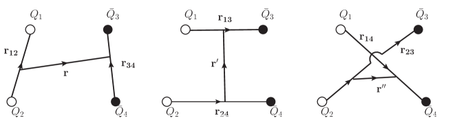
Figure 1: The Jacobi coordinates in the tetraquark state.

In a $Q_{1}Q_{2}\bar{Q}_{3}\bar{Q}_{4}$ tetraquark state, there are three sets of Jacobi coordinates as illustrated in Fig. 1. Each of them contains three independent Jacobi coordinates, and they can be transformed into others as follows,

$$\mathbf{r}_{jk}=\mathbf{r}_{j}-\mathbf{r}_{k}=\mathbf{r}+c_{jk}^{a}\mathbf{r}_{12}+c_{jk}^{b}\mathbf{r}_{34},$$

$$\mathbf{r}=\frac{m_{1}\mathbf{r}_{1}+m_{2}\mathbf{r}_{2}}{m_{1}+m_{2}}-\frac{m_{3}\mathbf{r}_{3}+m_{4}\mathbf{r}_{4}}{m_{3}+m_{4}},$$

$$\mathbf{r}^{\prime}=\frac{m_{1}\mathbf{r}_{1}+m_{3}\mathbf{r}_{3}}{m_{1}+m_{3}}-\frac{m_{2}\mathbf{r}_{2}+m_{4}\mathbf{r}_{4}}{m_{2}+m_{4}}$$

$$=\frac{(m_{1}m_{3}-m_{2}m_{4})\mathbf{r}+M_{T}u_{12}\mathbf{r}_{12}-M_{T}u_{34}\mathbf{r}_{34}}{(m_{1}+m_{4})(m_{2}+m_{3})},$$

$$\mathbf{r}^{\prime\prime}=\frac{m_{1}\mathbf{r}_{1}+m_{4}\mathbf{r}_{4}}{m_{1}+m_{4}}-\frac{m_{2}\mathbf{r}_{2}+m_{3}\mathbf{r}_{3}}{m_{2}+m_{3}}$$

$$=\frac{({m_{1}}{m_{4}}-m_{2}m_{3})\mathbf{r}+M_{T}u_{12}\mathbf{r}_{12}-M_{T}u_{34}\mathbf{r}_{34}}{(m_{1}+m_{3})(m_{2}+m_{4})},$$ (10)

where $M_{T}=\sum^{4}_{i=1}m_{i}$ is the total mass of the four quarks. The transformation coefficients $c^{a(b)}_{jk}$ are listed in Table 3. The superscripts $a$ and $b$ represent the quark cluster and antiquark cluster, respectively.

Table 3: The coefficient $c_{ij}$ in Eq. (II.2).

$c_{14}^{a}$	$c_{13}^{a}$	$c_{23}^{a}$	$c_{24}^{a}$	$c_{14}^{b}$	$c_{13}^{b}$	$c_{23}^{b}$	$c_{24}^{b}$
$\frac{m_{2}}{m_{1}+m_{2}}$	$\frac{m_{2}}{m_{1}+m_{2}}$	$-\frac{m_{1}}{m_{1}+m_{2}}$	$-\frac{m_{1}}{m_{1}+m_{2}}$	$\frac{m_{3}}{m_{3}+m_{4}}$	$-\frac{m_{4}}{m_{3}+m_{4}}$	$-\frac{m_{4}}{m_{3}+m_{4}}$	$\frac{m_{3}}{m_{3}+m_{4}}$

To simplify the calculation, we use the first coordinate configuration to construct the wave function considering the symmetry of the inner quarks. The wave function of a tetraquark state is

$$\psi_{JJ_{z}}=$$

$$\sum\left[\varphi_{n_{a}J_{a}}(\mathbf{r}_{12},\beta_{a})\otimes\varphi_{n_{b}J_{b}}(\mathbf{r}_{34},\beta_{b})\otimes\phi_{NL_{ab}}(\mathbf{r},\beta)\right]_{JJ_{z}},$$

$$\varphi_{n_{a}J_{a}M_{a}}=\left[\phi_{n_{a}l_{a}}(\mathbf{r}_{12},\beta_{a})\chi_{s_{a}}\right]_{M_{a}}^{J_{a}}\chi_{f}\chi_{c_{a}},$$ (11)

where the $\psi$ is the total wave function of the tetraquark state, and $\varphi$ denotes that of the cluster (a) or (b). $J$ ($J_{z}$) is the total angular momentum (the third direction component) of a tetraquark state. The $\sum$ is the sum over all the possible wave functions which may couple to the definite angular momentum $J$. $n_{a(b)}$ and $N$ specify the radial dependence. The $s_{a(b)}$, $l_{a(b)}$ and $J_{a(b)}$ are the spin, orbital and total angular momentum of the cluster $a$ ($b$). $L_{ab}$ is the orbital angular momentum between the two clusters. The $\chi_{s}$, $\chi_{f}$, $\chi_{c}$ are the wave functions in the spin, the isospin, and the color space, respectively. $\phi$ is the spatial wave function and is expressed by the Gaussian basis Hiyama:2003cu ,

$$\phi_{n_{a}l_{a}{m_{a}}}(\mathbf{r}_{12},\beta_{a}) = i^{l_{a}}r_{12}^{l_{a}}\sqrt{\frac{4\pi}{(2l_{a}+1)!!}}(\frac{n_{a}\beta_{a}^{2}}{\pi})^{3/4}$$

$$\times (2n_{a}\beta_{a}^{2})^{l_{a}/2}e^{-r^{2}\beta_{a}^{2}n_{a}/2}Y_{l_{a}m_{a}}(\mathbf{\Omega}_{12}).$$

with $\beta_{a}$ being the oscillating parameter.

In this work, we concentrate on the $S$-wave tetraquark states. Their wave functions are expanded by the basis which satisfies the relation $\mathbf{l}_{a}+\mathbf{l}_{b}+\mathbf{L}_{ab}=\mathbf{0}$. The states with higher orbital excitations contribute to the ground state through the tensor or the spin-orbital potentials. These contributions are higher order effects and neglected in this work. Thus, for the lowest $S$-wave tetraquark states, we only consider the wave functions with $l_{a}=l_{b}={L}_{ab}=0$. The wave function of the tetraquark state in Eq. (II.2) is simplified as

$$\psi_{SS_{z}} = \sum_{\alpha_{,}n_{A},n_{b},n_{ab}}\chi_{\alpha}\phi_{n_{a}}(\mathbf{r}_{12},\beta_{a})\phi_{n_{b}}(\mathbf{r}_{34},\beta_{b})\phi_{n_{ab}}(\mathbf{r},\beta),$$

$$\chi_{\alpha} = \left[\chi_{s_{a}}\otimes\chi_{s_{b}}\right]^{S}\left[\chi_{f_{a}}\otimes\chi_{f_{b}}\right]\left[\chi_{c_{a}}\otimes\chi_{c_{b}}\right]^{1},$$ (12)

where $S$ is the total spin of the tetraquark state and $1$ represents the color-singlet representation. For the spatial wave functions, we have omitted the orbital angular momentum in the Gaussian wave function $\phi$.

The wave functions are constrained by the Pauli principle. The $S$-wave diquark (antidiquark) with two identical quarks (antiquarks) has two possible configurations as listed in Table 4. Then, for the $cc\bar{c}\bar{c}$, $bb\bar{b}\bar{b}$, and $bb\bar{c}\bar{c}$ tetraquark states, the possible color-flavor-spin functions read

• $J^{PC}=0^{++}$

  $$\chi_{1}=\left[[QQ]_{\bar{3}_{c}}^{1}[\bar{Q}\bar{Q}]_{3_{c}}^{1}\right]_{1_{c}}^{0},\,\,\,\chi_{2}=\left[[QQ]_{6_{c}}^{0}[\bar{Q}\bar{Q}]_{\bar{6}_{c}}^{0}\right]_{1_{c}}^{0}.$$ (13)

• $J^{PC}=1^{+-}$

  $$\chi_{1}=\left[[QQ]_{\bar{3}_{c}}^{1}[\bar{Q}\bar{Q}]_{3_{c}}^{1}\right]_{1_{c}}^{1}.$$ (14)

• $J^{PC}=2^{++}$

  $$\chi_{1}=\left[[QQ]_{\bar{3}_{c}}^{1}[\bar{Q}\bar{Q}]_{3_{c}}^{1}\right]_{1_{c}}^{2}.$$ (15)

where the superscript and subscript denote the spin and color representations.

II.3 Hamiltonian matrix elements

Table 4: The configurations of the diquark (antiquark) constrained by Pauli principle. “S” and “A” represent symmetry and antisymmetry.

$J^{P}=1^{+}$	$QQ$	$J^{P}=0^{+}$	$QQ$
$S$-wave(L=0)	S	$S$-wave(L=0)	S
Flavor	S	Flavor	S
Spin(S=1)	S	Spin(S=0)	A
Color($\bar{3}_{c}$)	A	Color($6_{c}$)	S

With the wave function constructed in section II.2, we calculate the Hamiltonian matrix elements. For the quark model I, the matrix element of $\langle h_{12}\rangle$ reads,

$$\langle\chi_{\alpha_{i}}\phi_{n}(r_{12})\phi_{\lambda}(r_{34})\phi_{k}(r)|h_{12}|\chi_{\alpha_{j}}\phi_{m}(r_{12})\phi_{\nu}(r_{34})\phi_{k^{\prime}}(r)\rangle$$

$$=\delta_{\alpha_{i}\alpha_{j}}N_{\lambda,\nu}N_{k,k^{\prime}}\langle\phi_{n}(r_{12},\beta_{a})|h_{12}|\phi_{m}(r_{12},\beta_{a})\rangle$$

$$=\delta_{\alpha_{i}\alpha_{j}}N_{\lambda,\nu}N_{k,k^{\prime}}\left(\langle T_{12}+m_{1}+m_{2}\rangle+\langle V_{12}\rangle\right),$$ (16)

with

$$N_{k,k^{\prime}}=\left(\frac{2\sqrt{kk^{\prime}}}{k+k^{\prime}}\right)^{3/2},$$

$$\langle T_{12}+m_{1}+m_{2}\rangle=N_{m,n}\left(\frac{3mn\beta_{a}^{2}}{2u_{12}(m+n)}+m_{1}+m_{2}\right),$$

$$\langle V_{12}(\mathbf{r}_{12})\rangle=\langle V_{\text{coul}}\rangle+\langle V_{\text{conf}}\rangle+\langle V_{\text{hyp}}\rangle+\langle V_{\text{cons}}\rangle,$$

$$\langle V_{\text{coul}}\rangle=I_{C}\frac{4\pi\alpha_{s}\beta_{a}}{(2\pi)^{3/2}}\sqrt{m+n}N_{m,n},$$

$$\langle V_{\text{conf}}\rangle=-\frac{3}{4}I_{C}\frac{8\pi b}{(2\pi)^{3/2}\beta_{a}\sqrt{m+n}}N_{m,n},$$

$$\langle V_{\text{hyp}}\rangle=-I_{CM}\frac{8\pi\alpha_{s}}{3m_{i}m_{j}}\frac{\sigma^{3}}{\pi^{3/2}}\left(\frac{2\sqrt{mn}}{m+n+2\sigma^{2}/\beta_{a}^{2}}\right)^{\frac{3}{2}},$$

$$\langle V_{\text{cons}}\rangle=I_{C}V_{\text{cons}}N_{m,n},$$ (17)

where $n,\lambda,k,m,\nu,k^{\prime}$ specify the radial dependence. The $I_{C}$ and $I_{\text{CM}}$ are the color factor and the color electromagnetic factor in Table 5 and Table 6, respectively. $\chi_{\alpha_{i},\alpha_{j}}$ denote the color-flavor-spin configurations as illustrated in Eq. (II.2). Since the potential $h_{12}$ is diagonal in the color-flavor-spin space, it does not induce the coupling of different $\chi_{\alpha_{i},\alpha_{j}}$ channels and the $\langle h_{12}\rangle$ is proportional to $\delta_{\alpha_{i}\alpha_{j}}$. The derivation of $\langle h_{34}\rangle$ is similar to that of $\langle h_{12}\rangle$.

Table 5: The color matrix element $I_{C}=\langle\frac{\mathbf{\lambda}_{i}}{2}\frac{\mathbf{\lambda}_{j}}{2}\rangle$ for the $(ij)$ pair of quarks. The subscripts denote the color representation of the cluster.

$\langle(Q_{1}Q_{2})_{\bar{3}}(\bar{Q}_{3}\bar{Q}_{4})_{3}|\frac{\mathbf{\lambda}_{i}}{2}\frac{\mathbf{\lambda}_{j}}{2}|(Q_{1}Q_{2})_{\bar{3}}(\bar{Q}_{3}\bar{Q}_{4})_{3}\rangle$
$Q_{1}\bar{Q}_{3}$	$Q_{2}\bar{Q}_{4}$	$Q_{1}\bar{Q}_{4}$	$Q_{2}\bar{Q}_{3}$	$Q_{1}Q_{2}$	$\bar{Q}_{3}\bar{Q}_{4}$
$-\frac{1}{3}$	$-\frac{1}{3}$	$-\frac{1}{3}$	$-\frac{1}{3}$	$-\frac{2}{3}$	$-\frac{2}{3}$
$\langle(Q_{1}Q_{2})_{6}(\bar{Q}_{3}\bar{Q}_{4})_{\bar{6}}|\frac{\mathbf{\lambda}_{i}}{2}\frac{\mathbf{\lambda}_{j}}{2}|(Q_{1}Q_{2})_{6}(\bar{Q}_{3}\bar{Q}_{4})_{\bar{6}}\rangle$
$Q_{1}\bar{Q}_{3}$	$Q_{2}\bar{Q}_{4}$	$Q_{1}\bar{Q}_{4}$	$Q_{2}\bar{Q}_{3}$	$Q_{1}Q_{2}$	$\bar{Q}_{3}\bar{Q}_{4}$
$-\frac{5}{6}$	$-\frac{5}{6}$	$-\frac{5}{6}$	$-\frac{5}{6}$	$\frac{1}{3}$	$\frac{1}{3}$
$\langle(Q_{1}Q_{2})_{\bar{3}}(\bar{Q}_{3}\bar{Q}_{4})_{3}|\frac{\mathbf{\lambda}_{i}}{2}\frac{\mathbf{\lambda}_{j}}{2}|(Q_{1}Q_{2})_{6}(\bar{Q}_{3}\bar{Q}_{4})_{\bar{6}}\rangle$
$Q_{1}\bar{Q}_{3}$	$Q_{2}\bar{Q}_{4}$	$Q_{1}\bar{Q}_{4}$	$Q_{2}\bar{Q}_{3}$	$Q_{1}Q_{2}$	$\bar{Q}_{3}\bar{Q}_{4}$
$-\frac{1}{\sqrt{2}}$	$-\frac{1}{\sqrt{2}}$	$\frac{1}{\sqrt{2}}$	$\frac{1}{\sqrt{2}}$	$0$	$0$

Table 6: The color magnetic factor $\langle I_{\text{CM}}\rangle_{\alpha_{i}\alpha_{j}}=\langle\chi_{\alpha_{i}}|\frac{\lambda_{i}}{2}\frac{\lambda_{j}}{2}\mathbf{s}_{i}\cdot\mathbf{s}_{j}|\chi_{\alpha_{j}}\rangle$ for the $(ij)$ quark pairs. The $\chi_{\alpha_{i,j}}$ denotes the color-flavor-spin wave functions in Eqs. (13)-(15).

	$I_{CM}^{ij}=\langle\frac{\lambda_{i}}{2}\frac{\lambda_{j}}{2}s_{i}\cdot s_{j}\rangle$
$0^{++}$	$\langle I_{CM}^{Q\bar{Q}}\rangle_{11}$	$\langle I_{CM}^{QQ}\rangle_{11}$	$\langle I_{CM}^{\bar{Q}\bar{Q}}\rangle_{11}$
	$\frac{1}{6}$	$-\frac{1}{6}$	$-\frac{1}{6}$
	$\langle I_{CM}^{Q\bar{Q}}\rangle_{22}$	$\langle I_{CM}^{QQ}\rangle_{22}$	$\langle I_{CM}^{QQ}\rangle_{22}$
	$0$	$-\frac{1}{4}$	$-\frac{1}{4}$
	$\langle I_{CM}^{Q\bar{Q}}\rangle_{12}$	$\langle I_{CM}^{QQ}\rangle_{11}$	$\langle I_{CM}^{\bar{Q}\bar{Q}}\rangle_{11}$
	$\frac{\sqrt{3}}{4\sqrt{2}}$	$0$	$0$
$1^{+-}$	$\langle I_{CM}^{Q\bar{Q}}\rangle_{11}$	$\langle I_{CM}^{QQ}\rangle_{11}$	$\langle I_{CM}^{\bar{Q}\bar{Q}}\rangle_{11}$
	$\frac{1}{12}$	$-\frac{1}{6}$	$-\frac{1}{6}$
$2^{++}$	$\langle I_{CM}^{Q\bar{Q}}\rangle_{11}$	$\langle H_{CM}^{QQ}\rangle_{11}$	$\langle H_{CM}^{\bar{Q}\bar{Q}}\rangle_{11}$
	$-\frac{1}{12}$	$-\frac{1}{6}$	$-\frac{1}{6}$

Unlike the $h_{12}$ and $h_{34}$, the $V_{I}(\mathbf{r}_{ij})$ with $i=1,2$ and $j=3,4$, which is the interaction between the diquark and antidiquark, may lead to the mixing between different color-spin-flavor configurations, i.e. $\chi_{\alpha_{i}}$ and $\chi_{\alpha_{j}}$. The $\langle V_{I}(\mathbf{r}_{ij})\rangle$ reads

$$\langle\chi_{\alpha_{i}}\phi_{n}(r_{12},\beta_{a})\phi_{\lambda}(r_{34},\beta_{b})\phi_{k}(r,\beta)|V_{I}(\mathbf{r}_{ij})$$

$$|\chi_{\alpha_{j}}\phi_{m}(r_{12},\gamma_{a})\phi_{\nu}(r_{34},\gamma_{b})\phi_{k^{\prime}}(r,\gamma)\rangle$$

$$=\langle V_{\text{coul}}(\mathbf{r}_{ij})\rangle_{\alpha_{i}\alpha_{j}}+\langle V_{\text{conf}}(\mathbf{r}_{ij})\rangle_{\alpha_{i}\alpha_{j}}+\langle V_{\text{hyp}}(\mathbf{r}_{ij})\rangle_{\alpha_{i}\alpha_{j}},$$

where ${\beta_{(a,b)}}$ and $\gamma_{{(a,b)}}$ are the oscillating parameters. The implicit forms of the notations are

$$\langle V_{\text{coul}}(\mathbf{r}_{ij})\rangle=I_{C}\tilde{N}_{m,n}\tilde{N}_{\lambda,\nu}\tilde{N}_{k,k^{\prime}}\frac{2\alpha_{s}}{\sqrt{\pi}\sqrt{\frac{2}{k\beta^{2}+k^{\prime}\gamma^{2}}+4a_{ij}^{2}}},$$

$$\langle V_{\text{conf}}(\mathbf{r}_{ij})\rangle=I_{C}\tilde{N}_{m,n}\tilde{N}_{\lambda,\nu}\tilde{N}_{k,k^{\prime}}(-\frac{3bz_{ij}}{\sqrt{\pi}}),$$

$$\langle V_{\text{hyp}}(\mathbf{r}_{ij})\rangle=I_{CM}\tilde{N}_{m,n}\tilde{N}_{\lambda,\nu}{\tilde{N}_{k,k^{\prime}}}$$

$$~{}~{}~{}~{}~{}~{}~{}~{}~{}~{}~{}~{}~{}\times\left(-\frac{8\alpha_{s}}{3m_{i}m_{j}(4\tau_{ij}^{2}+\frac{2}{k\beta^{2}+k^{\prime}\gamma^{2}})^{3/2}\sqrt{\pi}}\right),$$ (18)

where

$$\tilde{N}_{m,n}=\left({2\sqrt{mn}\beta_{a}\gamma_{a}\over{m\gamma_{a}^{2}+n\beta_{a}^{2}}}\right)^{3/2},$$ (19)

$$a_{ij}=\frac{(c_{ij}^{a})^{2}}{2(m\beta_{a}^{2}+n{\gamma_{a}}^{2})}+\frac{(c_{ij}^{b})^{2}}{2(\lambda\beta_{b}^{2}+\nu\gamma_{b}^{2})},$$ (20)

$$\tau_{ij}^{2}=a_{ij}^{2}+\frac{1}{4\sigma^{2}},\,\,z_{ij}^{2}=a_{ij}^{2}+\frac{1}{2(k\beta^{2}+k^{\prime}\gamma^{2})}.$$ (21)

With the above analytical expressions, we calculate the mass spectrum of the fully heavy tetraquark states $QQ\bar{Q}^{\prime}\bar{Q}^{\prime}$. The numerical results are given in the next section.

III Numerical results

The wave function of a tetraquark state is composed of all wave functions which subject to the conditions discussed in section II.2. The number of the basis $N^{3}$ increases from the minimum required to a large limit. We take the $cc\bar{c}\bar{c}$ tetraquark state with $J^{PC}=1^{+-}$ as an example to investigate the dependence of the results on the number of the basis. Its wave function is expanded with $N^{3}=1^{3}$, $2^{3}$, $3^{3}$, $4^{3}$ and $5^{3}$ basis, respectively. The corresponding eigenvalues obtained through the variational method are displayed in Fig. 2. The mass spectrum tends to be stable when $N^{3}$ is larger than $2^{3}$. Therefore, we expand the wave functions of the tetraquark states with $2^{3}$ Gaussian basis in the following calculation.

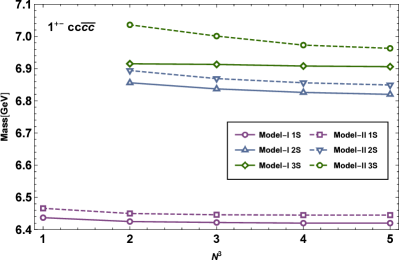
Figure 2: The dependence of the mass spectrum on the number of Gaussian basis $N^{3}$. The line and dashed line represent the numerical results in model I and model II, respectively.

III.1 A tetraquark state $QQ\bar{Q}^{\prime}\bar{Q}^{\prime}$ with $J^{PC}=0^{++}$

A tetraquark state $QQ\bar{Q}^{\prime}\bar{Q}^{\prime}$ with $J^{PC}=0^{++}$ contains two color-flavor-spin configurations $\chi_{1}$ and $\chi_{2}$ as listed in Eq. (13). Its wave function reads

$$\psi_{JJ_{z}}^{II_{z}}=\sum_{\alpha_{1}}A_{\alpha_{1}}\phi_{\alpha_{1}}\chi_{1}+\sum_{\alpha_{2}}B_{\alpha_{2}}\phi_{\alpha_{2}}\chi_{2}$$

$$=\sum_{\alpha_{1}}A_{\alpha_{1}}\phi_{\alpha_{1}}(\beta_{a},\beta_{b},\beta)|(QQ)_{\bar{3}_{c}}(\bar{Q}\bar{Q})_{3_{c}}\rangle$$

$$+\sum_{\alpha_{2}}B_{\alpha_{2}}\phi_{\alpha_{2}}(\gamma_{a},\gamma_{b},\gamma)|(QQ)_{6_{c}}(\bar{Q}\bar{Q})_{\bar{6}_{c}}\rangle,$$ (22)

where $\alpha_{1,2}=\{n_{a},l_{a},n_{b},l_{b},N,L\}$, $\beta_{(a,b)}$ and $\gamma_{(a,b)}$ are the oscillating parameters for the $\bar{3}_{c}-3_{c}$ and $6_{c}-\bar{6}_{c}$ tetraquark states. $A_{\alpha_{1}}$ and $B_{\alpha_{2}}$ are the expanding coefficients.

At first, we do not consider the mixture between the $\bar{3}_{c}-3_{c}$ and $6_{c}-\bar{6}_{c}$ tetraquark states and solve the Schödinger equation with the variational method. We obtain their mass spectra and display them in the left panel of Fig. 3.

For the $cc\bar{c}\bar{c}$ and $bb\bar{b}\bar{b}$ systems, the $6_{c}-\bar{6}_{c}$ states are located lower than the $\bar{3}_{c}-3_{c}$ ones as illustrated in Fig. 3. In the OGE model, the interactions between the two quarks within a color-sextet diquark are repulsive due to the color factor in Table 5, while those in the $\bar{3}_{c}$ one is attractive. However, the interactions between the $6_{c}$ diquark and $\bar{6}_{c}$ antidiquark are attractive and much stronger than that between the $\bar{3}_{c}$ diquark and $3_{c}$ antidiquark. There exists a $6_{c}-\bar{6}_{c}$ tetraquark state, if the attraction between diquark and antidiquark wins against the repulsion within the diquak (antidiquark). If the attractive potentials are strong enough, the $6_{c}-\bar{6}_{c}$ state stays even lower than the ${\bar{3}_{c}}-{3_{c}}$ one. That is what happens to the $cc\bar{c}\bar{c}$, $bb\bar{b}\bar{b}$ tetraquark states with $J^{PC}=0^{++}$ in the two quark models. For the $bb\bar{c}\bar{c}$ ($cc\bar{b}\bar{b}$) state, the $6_{c}-\bar{6}_{c}$ state is lower in model I, while the $\bar{3}_{c}-3_{c}$ state is lower in model II.

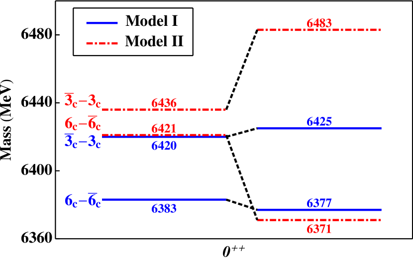
(a)  $cc\bar{c}\bar{c}$

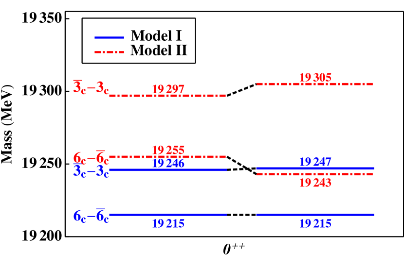
(b)  $bb\bar{b}\bar{b}$

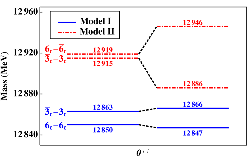
(c)  $bb\bar{c}\bar{c}$ ($cc\bar{b}\bar{b}$)

Figure 3: The mass spectrum of the $0^{++}$ tetraquark states $QQ\bar{Q}^{\prime}\bar{Q}^{\prime}$ without and with the coupling between the $\bar{3}_{c}-3_{c}$ and $6_{c}-\bar{6}_{c}$ configurations. The blue lines and red dotted dashed lines represent the results in model I and II, respectively. In every diagrams, the left half and the right half are the mass spectrum without and with mixing between $\bar{3}_{c}-3_{c}$ and $6_{c}-\bar{6}_{c}$ configurations, respectively. The corresponding states are connected by the black dashed lines.

Table 7: The mass spectra of $cc\bar{c}\bar{c}$, $bb\bar{b}\bar{b}$, and $bb\bar{c}\bar{c}$ ($\bar{b}\bar{b}cc$) tetraquark states with $J^{PC}=0^{++}$. $\beta_{(a,b)}$ and $\gamma_{(a,b)}$ represent the oscillating parameters of the $\bar{3}_{c}-3_{c}$ and $6_{c}-\bar{6}_{c}$ tetraquark states, respectively.

$J^{PC}=0^{++}$	Model I	M [GeV]	$\bar{3}_{c}\otimes 3_{c}$	$6_{c}\otimes\bar{6}_{c}$	Model II	M [GeV]	$\bar{3}_{c}\otimes 3_{c}$	$6_{c}\otimes\bar{6}_{c}$
$cc\bar{c}\bar{c}$	$\beta_{a}=\beta_{b}=0.4$, $\beta=0.6$	$6.377$	$11\%$	$89\%$	$\beta_{a}=\beta_{b}=0.5$, $\beta=0.7$	$6.371$	$43\%$	$57\%$
	$\gamma_{a}=\gamma_{b}=0.4$, $\gamma=0.7$	$6.425$	$89\%$	$11\%$	$\gamma_{a}=\gamma_{b}=0.5$, $\gamma=0.8$	$6.483$	$57\%$	$43\%$
$bb\bar{b}\bar{b}$	$\beta_{a}=\beta_{b}=0.7$, $\beta=0.9$	$19.215$	$1\%$	$99\%$	$\beta_{a}=\beta_{b}=0.9$, $\beta=1.1$	$19.243$	$17\%$	$83\%$
	$\gamma_{a}=\gamma_{b}=0.7$, $\gamma=0.9$	$19.247$	$99\%$	$1\%$	$\gamma_{a}=\gamma_{b}=0.8$, $\gamma=1.2$	$19.305$	$83\%$	$17\%$
$bb\bar{c}\bar{c}$	$\beta_{a}=0.6,\beta_{b}=0.5,\beta=0.7$	$12.847$	$14\%$	$86\%$	$\beta_{a}=0.7,\beta_{b}=0.5,\beta=0.8$	$12.886$	$53\%$	$47\%$
	$\gamma_{a}=0.6,\gamma_{b}=0.4,\gamma=0.9$	$12.866$	$86\%$	$14\%$	$\gamma_{a}=0.7,\gamma_{b}=0.5,\gamma=0.9$	$12.946$	$47\%$	$53\%$

In general, a tetraquark state is a mixture of the $\bar{3}_{c}-{3_{c}}$ and ${6_{c}}-{\bar{6}_{c}}$ states as illustrated in Eq. (22). With the couple-channel effects of the $\bar{3}_{c}-3_{c}$ and $6_{c}-\bar{6}_{c}$ color configurations, we obtain the mass spectrum of the $0^{++}$ states and list them in Table 7. The spectra obtained with $\bar{3}_{c}-{3_{c}}$ and ${6_{c}}-{\bar{6}_{c}}$ mixing are given in Fig. 3. The mixing effect will pull down the lower state and raise the higher state. The two quark models lead to similar mass spectra for the $cc\bar{c}\bar{c}$, $bb\bar{b}\bar{b}$, and $bb\bar{c}\bar{c}$ ($cc\bar{b}\bar{b}$) tetraquark states with the differences up to tens of MeV. However, the proportions of the components in the two quark models are quite different. The mixing between the $\bar{3}_{c}-3_{c}$ and $6_{c}-\bar{6}_{c}$ states are more stronger in model II. The reasons are explained as follows.

In model I and model II, we find that only the hyperfine interactions contribute to the couple-channel effects of the ${\bar{3}_{c}}-{3_{c}}$ configuration and the ${6_{c}}-{\bar{6}_{c}}$ one, while the contributions from the confinement and Coulomb potentials vanish. We illustrate the underlying dynamics as follows. The matrices of $h_{12}$ and $h_{34}$ are diagonal due to the orthogonality of the wave functions of different configurations. However, the $V_{\text{coul}}+V_{\text{linear}}+V_{\text{hyp}}$ in $V_{I}$, which describes the interactions between the diquark and antidiquark, may result in the couple-channel effects of different configurations. For an S-wave tetraquark state with two identical quarks (antiquarks), such as $QQ\bar{Q}_{1}\bar{Q}_{2}$ ($Q_{1}Q_{2}\bar{Q}\bar{Q}$), the spin wave functions of different possible configurations are orthogonal, which is constrained by the Fermi statistic. Since the OGE Coulomb and linear confinement potentials do not contain spin operators, they do not contribute to the couple-channel effects due to the orthogonality of the spin wave functions. And only the hyperfine potential contributes. That is what happens to the $QQ\bar{Q}^{\prime}\bar{Q}^{\prime}$ state in this work.

For a tetraquark state without identical quarks and antiquarks, i.e., $Q_{1}Q_{2}\bar{Q}_{3}\bar{Q}_{4}$ ($Q_{1}\neq Q_{2}$ and $Q_{3}\neq Q_{4}$), the spin wave functions of different configurations may be the same. The four quarks form a color singlet state and the color matrix element is

$$(\sum^{4}_{n}\mathbf{\lambda}_{n})^{2}|\chi_{i,j}\rangle=0.$$ (23)

where $\chi_{i}$ and $\chi_{j}$ represent two different color configurations and they are the eigenvectors of $\mathbf{\lambda}_{1}+\mathbf{\lambda}_{2}$ and $\mathbf{\lambda}_{3}+\mathbf{\lambda}_{4}$. Considering their orthogonality, one obtains

$$\langle\chi_{i}|(\mathbf{\lambda}_{1}+\mathbf{\lambda}_{2})^{2}|\chi_{j}\rangle=0,$$

$$\langle\chi_{i}|(\mathbf{\lambda}_{3}+\mathbf{\lambda}_{4})^{2}|\chi_{j}\rangle=0.$$ (24)

Then the color factors of the (13), (14), (23), and (24) pairs of quarks cancel out,

$$\langle\chi_{i}|(\lambda_{1}+\lambda_{2})(\lambda_{3}+\lambda_{4})|\chi_{j}\rangle=0.$$ (25)

Moreover, if the coupling constants are the same for the four quark pairs, the contributions from the OGE Coulomb and the linear confinement potentials will cancel out completely. In model I, the contributions from the color interactions do not cancel out exactly due to different $\alpha_{s}$. However, partial cancellations are still expected. In model II, the OGE Coulomb and linear confinement potentials do not depend on the mass of the interacting quarks. Thus, the couple-channel effects arising from the OGE Coulomb and linear confinement potentials cancel out. The mixing between different color-flavor-spin configurations only comes from the hyperfine potential, which is inversely proportional to the interacting quark mass. Thus, the mixing in the $cc\bar{c}\bar{c}$ state is generally larger than that in the $bb\bar{b}\bar{b}$ state.

In model II, all the flavor dependence is packaged into the hyperfine interaction, which is different from model I. The hyperfine interaction in model II should play a more important role than that in model I. Therefore, the couple-channel effect in model II is stronger as illustrated in Fig. 3.

In model II, since the $r_{0}$ in the hyperfine interaction is the function of the reduced mass between the two quarks, its value for $b\bar{c}$ is in proximity to that of $c\bar{c}$. Then, the mixing in $cc\bar{c}\bar{c}$ and $bb\bar{c}\bar{c}$ are similar as illustrated in Table 7. One may wonder the additional dependence of the mixing on the number of the expanding basis. For instance, when we use $2\times 3^{3}$ bases to expand the wave function of the $cc\bar{c}\bar{c}$ state in model I, we find there are $11.4\%$ $\bar{3}_{c}-3_{c}$ and $88.6\%$ $6_{c}-\bar{6}_{c}$ components in the tetraquark state. The percents change slightly with the number of the basis.

In Ref. Liu:2019zuc , the authors pointed out that the state $|(QQ)_{\bar{3}_{c}}(\bar{Q}\bar{Q})_{3_{c}}\rangle$ $(Q=c,b)$ is located lower than the $|(QQ)_{6_{c}}(\bar{Q}\bar{Q})_{\bar{6}_{c}}\rangle$ state, which contradicts with our results. The inconsistency was due to their use of particular wave functions. The authors used the same oscillating parameters for the $\bar{3}_{c}-3_{c}$ and $6_{c}-\bar{6}_{c}$ states. Moreover, the oscillating parameters are proportional to the reduced masses of the interacting quarks. With their wave function, we reproduced their results. However, if we remove the two constrains on the wave functions, we find the lowest state with a dominant ${6_{c}}-{\bar{6}_{c}}$ component as listed in Table 8, which is lower than that in Ref. Liu:2019zuc .

Table 8: The comparison of the mass spectra of $0^{++}$ $cc\bar{c}\bar{c}$ and $bb\bar{b}\bar{b}$ from Ref. Liu:2019zuc and our results using the same quark model. In the right table, we remove the constrains on the wave functions used in Ref. Liu:2019zuc .

	Ref. Liu:2019zuc				without constrains
$J^{PC}=0^{++}$	$w=0.325$	M [GeV]	$\bar{3}_{c}\otimes 3_{c}$	$6_{c}\otimes\bar{6}_{c}$		M [GeV]	$\bar{3}_{c}\otimes 3_{c}$	$6_{c}\otimes\bar{6}_{c}$
$cc\bar{c}\bar{c}$	$\beta_{a}=\beta_{b}=0.49$, $\beta=0.69$	$6470$	$66\%$	$34\%$	$\beta_{a}=\beta_{b}=0.4$, $\beta=0.6$	$6417$	$33\%$	$67\%$
	$\gamma_{a}=\gamma_{b}=0.49$, $\gamma=0.69$	$6559$	$34\%$	$66\%$	$\gamma_{a}=\gamma_{b}=0.4$, $\gamma=0.7$	$6509$	$67\%$	$33\%$
$bb\bar{b}\bar{b}$	$\beta_{a}=\beta_{b}=0.88$, $\beta=1.24$	$19268$	$66\%$	$34\%$	$\beta_{a}=\beta_{b}=0.7$, $\beta=0.9$	$19226$	$18\%$	$82\%$
	$\gamma_{a}=\gamma_{b}=0.88$, $\gamma=1.24$	$19306$	$34\%$	$66\%$	$\gamma_{a}=\gamma_{b}=0.7$, $\gamma=0.9$	$19268$	$82\%$	$18\%$

III.2 The tetraquark states with $J^{P}=1^{+-}$ and $2^{++}$

Constrained by the Fermi statistics, the tetraquark states $QQ\bar{Q}^{\prime}\bar{Q}^{\prime}$ ($Q$ and $Q^{\prime}$ may be the same flavors) with $J^{P}=1^{+-}$ and $2^{++}$ only contain one color component, i.e. $\bar{3}_{c}-3_{c}$. We list the mass spectra of the $S$-wave states and their radial excitations in Table 9. The mass spectra in the two models are quite similar to each other. The results from Model II are slightly higher than those in Model I.

The tetraquark states with $J^{P}=1^{+-}$ and $2^{++}$ have the same configurations except the total spin. Therefore, the mass difference arises from the hyperfine potential, which is quite small compared with the OGE Coulomb and linear confinement potentials. Thus, the mass spectra of these two kinds of states are almost the same.

Table 9: The mass spectra of the $cc\bar{c}\bar{c}$, $bb\bar{b}\bar{b}$ and $bb\bar{c}\bar{c}$ states with $J^{PC}=1^{+-}$ and $2^{++}$ in units of GeV.

	Model I	$nS$	$J^{PC}=1^{+-}$	$J^{PC}=2^{++}$	Model II	$nS$	$J^{PC}=1^{+-}$	$J^{PC}=2^{++}$
$cc\bar{c}\bar{c}$	$\beta_{a}=0.4$	$1S$	$6.425$	$6.432$	$\beta_{a}=0.5$	$1S$	$6.450$	$6.479$
	$\beta_{b}=0.4$	$2S$	$6.856$	$6.864$	$\beta_{b}=0.5$	$2S$	$6.894$	$6.919$
	$\beta=0.6$	$3S$	$6.915$	$6.919$	$\beta=0.6$	$3S$	$7.036$	$7.058$
$bb\bar{b}\bar{b}$	$\beta_{a}=0.7$	$1S$	$19.247$	$19.249$	$\beta_{a}=1.0$	$1S$	$19.311$	$19.325$
	$\beta_{b}=0.7$	$2S$	$19.594$	$19.596$	$\beta_{b}=1.0$	$2S$	$19.813$	$19.823$
	$\beta=0.9$	$3S$	$19.681$	$19.682$	$\beta=1.1$	$3S$	$20.065$	$20.077$
$bb\bar{c}\bar{c}$	$\beta_{a}=0.7$	$1S$	$12.864$	$12.868$	$\beta_{a}=0.7$	$1S$	$12.924$	$12.940$
	$\beta_{b}=0.5$	$2S$	$13.259$	$13.262$	$\beta_{b}=0.5$	$2S$	$13.321$	$13.334$
	$\beta=0.7$	$3S$	$13.297$	$13.299$	$\beta=0.7$	$3S$	$13.364$	$13.375$

III.3 Disscussion

A tetraquark state can be expressed in another set of color representations as follows,

$$|(Q_{1}Q_{2})_{\bar{3}_{c}}(\bar{Q}_{3}\bar{Q}_{4})_{3_{c}}\rangle$$

$$=\sqrt{\frac{1}{3}}|(Q_{1}\bar{Q}_{3})_{1_{c}}(Q_{2}\bar{Q}_{4})_{1_{c}}\rangle-\sqrt{\frac{2}{3}}|(Q_{1}\bar{Q}_{3})_{8_{c}}(Q_{2}\bar{Q}_{4})_{8_{c}}\rangle$$

$$=-\sqrt{\frac{1}{3}}|(Q_{1}\bar{Q}_{4})_{1_{c}}(Q_{2}\bar{Q}_{3})_{1_{c}}\rangle+\sqrt{\frac{2}{3}}|(Q_{1}\bar{Q}_{4})_{8_{c}}(Q_{2}\bar{Q}_{3})_{8_{c}}\rangle,$$

$$|(Q_{1}Q_{2})_{6_{c}}(\bar{Q}_{3}\bar{Q}_{4})_{\bar{6}_{c}}\rangle$$

$$=\sqrt{\frac{2}{3}}|(Q_{1}\bar{Q}_{3})_{1_{c}}(Q_{2}\bar{Q}_{4})_{1_{c}}\rangle+\sqrt{\frac{1}{3}}|(Q_{1}\bar{Q}_{3})_{8_{c}}(Q_{2}\bar{Q}_{4})_{8_{c}}\rangle$$

$$=\sqrt{\frac{2}{3}}|(Q_{1}\bar{Q}_{4})_{1_{c}}(Q_{2}\bar{Q}_{3})_{1_{c}}\rangle+\sqrt{\frac{1}{3}}|(Q_{1}\bar{Q}_{4})_{8_{c}}(Q_{2}\bar{Q}_{3})_{8_{c}}\rangle.$$

To investigate the inner structure of the tetraquark, we calculate its proportions in the new set and the root mean square radii of the state, which are listed in Table 10. The ground states contain the $8_{c}\otimes 8_{c}$ configuration. In model I, the proportion of the $8_{c}\otimes 8_{c}$ configuration is considerable, which supports that the solution is a confined state rather than a scattering state of two mesons. In model II, though the $1_{c}\otimes 1_{c}$ configuration is dominant, the root mean square radii are of the size of nucleons. Thus, they are also unlikely to be scattering states.

We also take the $cc\bar{c}\bar{c}$ as an example to study the density distributions of $r^{2}\rho(r)$, $r^{2}\rho(r^{\prime})$, $r^{2}_{12}\rho(r_{12})$ and $r^{2}_{13}\rho(r_{13})$. The $\rho(r)$ and $\rho(r_{12})$ are defined as follows,

$$\rho(r)={\int}|\psi(r_{12},\,r_{34},\,r)|{}^{2}d\vec{r}_{12}d\vec{r}_{34}d\hat{\vec{r}},$$

$$\rho(r_{12})=\int|\psi(r_{12},\,r_{34},\,r)|{}^{2}d\vec{r}d\vec{r}_{34}d\hat{\vec{r}}_{12}.$$ (27)

The definitions of the $\rho(r_{13})$ and $\rho(r^{\prime})$ are similar. The dependence of the density distributions on the extension of the basis function is displayed in Fig. 4. We find that the distributions are confined in the spatial space and tend to be stable with different number of the expanding basis, which indicates the state may be a confined state instead of a scattering state.

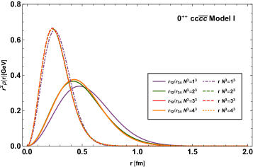
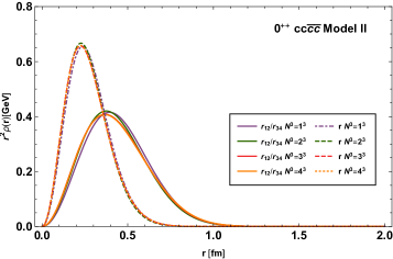
(a)  Density distributions in the first Jacobi coordinate.

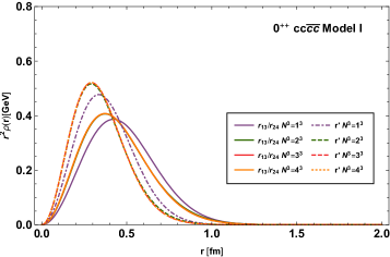
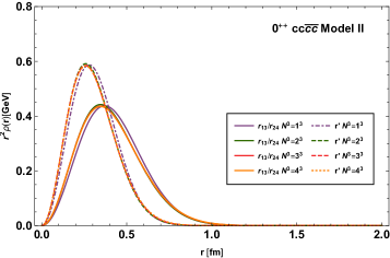
(b)  Density distributions in the second Jacobi coordinate.

Figure 4: The dependence of density distributions on the number of the basis functions.

Table 10: The proportion of the color configurations and the root mean square radii of the $cc\bar{c}\bar{c}$, $bb\bar{b}\bar{b}$, and $bb\bar{c}\bar{c}$ ($\bar{b}\bar{b}cc$) tetraquark states with $J^{PC}=0^{++}$. $\sqrt{\langle r_{ij}^{2}\rangle}$ and $\sqrt{\langle r^{(^{\prime})2}\rangle}$ are the root mean square radii corresponding to the second Jacobi coordinate in Fig. 1.

$J^{PC}=0^{++}$	Model I
$N^{3}=2^{3}$	After mixing	$\bar{3}_{c}\otimes 3_{c}$	$6_{c}\otimes\bar{6}_{c}$	$1_{c}\otimes 1_{c}$	$8_{c}\otimes 8_{c}$	$\sqrt{\langle r_{12}^{2}\rangle}$ fm	$\sqrt{\langle r_{34}^{2}\rangle}$ fm	$\sqrt{\langle r^{2}\rangle}$ fm	$\sqrt{\langle r_{13}^{2}\rangle}$ fm	$\sqrt{\langle r_{24}^{2}\rangle}$ fm	$\sqrt{\langle r^{\prime 2}\rangle}$ fm
$cc\bar{c}\bar{c}$	$6.377$	$11\%$	$89\%$	$90\%$	$10\%$	$0.54$		$0.30$	$0.49$		$0.38$
$bb\bar{b}\bar{b}$	$19.215$	$1\%$	$99\%$	$75\%$	$25\%$	$0.35$		$0.19$	$0.31$		$0.25$
$bb\bar{c}\bar{c}$	$12.847$	$14\%$	$86\%$	$92\%$	$8\%$	$0.39$	$0.50$	$0.26$	$0.41$		$0.32$
Model II
$N^{3}=2^{3}$	After mixing	$\bar{3}_{c}\otimes 3_{c}$	$6_{c}\otimes\bar{6}_{c}$	$1_{c}\otimes 1_{c}$	$8_{c}\otimes 8_{c}$	$\sqrt{\langle r_{12}^{2}\rangle}$ fm	$\sqrt{\langle r_{34}^{2}\rangle}$ fm	$\sqrt{\langle r^{2}\rangle}$ fm	$\sqrt{\langle r_{13}^{2}\rangle}$ fm	$\sqrt{\langle r_{24}^{2}\rangle}$ fm	$\sqrt{\langle r^{\prime 2}\rangle}$ fm
$cc\bar{c}\bar{c}$	$6.371$	$43\%$	$57\%$	$97\%$	$3\%$	$0.47$		$0.30$	$0.45$		$0.33$
$bb\bar{b}\bar{b}$	$19.243$	$17\%$	$83\%$	$94\%$	$6\%$	$0.28$		$0.17$	$0.26$		$0.20$
$bb\bar{c}\bar{c}$	$12.886$	$53\%$	$47\%$	$93\%$	$7\%$	$0.32$	$0.44$	$0.26$	$0.37$		$0.26$

We present the mass spectra of the tetraquark states and the mass thresholds of possible scattering states in Fig. 5. As illustrated in this figure, the $bb\bar{b}\bar{b}$, $cc\bar{c}\bar{c}$, and $bb\bar{c}\bar{c}$ states with $J^{PC}=0^{++}$ are the lowest states. But they are still located above the corresponding meson-meson mass thresholds, which indicates that there may not exist bound states in the two quark models.

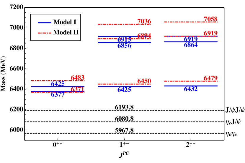
(a)  $cc\bar{c}\bar{c}$

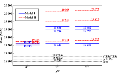
(b)  $bb\bar{b}\bar{b}$

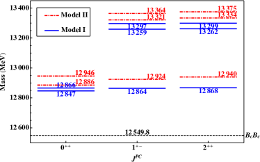
(c)  $bb\bar{c}\bar{c}(cc\bar{b}\bar{b})$.

Figure 5: The mass spectra of the $cc\bar{c}\bar{c}$, $bb\bar{b}\bar{b}$, and $bb\bar{c}\bar{c}(cc\bar{b}\bar{b})$ tetraquark states. The blue line and red dotted dashed line represent the results in model I and II, respectively.

We also investigate the constituent quark mass dependence of the tetraquark spectra. We vary the quark mass and display the results in Fig. 6. The figure shows that both the tetraquark mass and the $\eta_{Q}\eta_{Q}$ threshold increase with the quark mass. The $QQ\bar{Q}\bar{Q}$ is always located above the mass thresholds of the $\eta_{Q}\eta_{Q}$ and no bound tetraquark states exist.

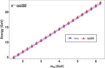
(a) The mass spectra of the tetraquark states $QQ\bar{Q}\bar{Q}$ with $J^{PC}=0^{++}$.

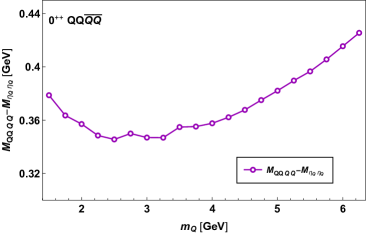
(b) The mass difference between the tetraquark states and the mass threshold of $\eta_{Q}\eta_{Q}$.

Figure 6: The quark mass dependence of the $0^{++}$ tetraquark states $QQ\bar{Q}\bar{Q}$ in model II. In this figure, we use the $\eta_{Q}$ to denote the meson state $Q\bar{Q}$ with $J^{PC}=0^{-+}$.

IV Summary

In this work, we have systematically calculated the mass spectra of the tetraquark states $cc\bar{c}\bar{c}$, $bb\bar{b}\bar{b}$, and $bb\bar{c}\bar{c}$ in two nonrelativistic quark models, which contain the OGE Coulomb, linear confinement and hyperfine potentials.

For a $QQ\bar{Q}^{\prime}\bar{Q}^{\prime}$ ($Q$ and $Q^{\prime}$ may be the same flavors) state with $J^{PC}=0^{++}$, it can be formed by a $6_{c}$ diquark and a $\bar{6}_{c}$ antidiquark, or a $\bar{3}_{c}$ diquark and a $3_{c}$ antidiquark. For the tetraquark states $cc\bar{c}\bar{c}$ and $bb\bar{b}\bar{b}$, the $6_{c}-\bar{6}_{c}$ states are located lower than the $\bar{3}_{c}-3_{c}$ ones due to the strong attractions between the diquark and the antidiquark. For the $bb\bar{c}\bar{c}$ ($cc\bar{b}\bar{b}$), the mass of the $6_{c}-\bar{6}_{c}$ state is lower than that of the $\bar{3}_{c}-3_{c}$ one in the model I, while the $\bar{3}_{c}-3_{c}$ one is lower in the model II. Our calculation shows that the $6_{c}-\bar{6}_{c}$ color configuration is important and sometimes even dominant in the formation of fully heavy tetraquark states. One should be cautious about neglecting the $6_{c}-\bar{6}_{c}$ color configurations in calculating the tetraquark states.

The $6_{c}-\bar{6}_{c}$ configuration couples with the $\bar{3}_{c}-3_{c}$ one through the interactions between the diquark and antidiquark. For a $QQ\bar{Q}^{\prime}\bar{Q}^{\prime}$ state, we prove that only the hyperfine potential contributes to the mixing between the two configurations, while the contributions from the OGE Coulomb and the linear confinement potentials cancel out exactly.

Table 11: The mass spectra (in units of GeV) of the tetraquark states $cc\bar{c}\bar{c}$, $bb\bar{b}\bar{b}$, and $bb\bar{c}\bar{c}$ in different frameworks. The $M^{1}_{th}$ and $M^{2}_{th}$ are the numerical results from the quark model I and II in this work, respectively.

	$J^{PC}$	$M_{th}^{1}$	$M_{th}^{2}$	Berezhnoy:2011xn	Karliner:2016zzc	Wu:2016vtq	Anwar:2017toa	Bai:2016int	Barnea:2006sd	Liu:2019zuc	Chen:2016jxd ; Chen:2018cqz
	$0^{++}$	$6.377$	$6.371$	$5.966$	$6.192\pm 0.025$	$6.001$	$...$	$...$	$6.038$	$6.470$	$6.44\pm 0.15$
$cc\bar{c}\bar{c}$		$6.425$	$6.483$							$6.558$
	$1^{+-}$	$6.425$	$6.450$	$6.051$	$...$	$6.109$	$...$	$...$	$6.101$	$6.512$	$6.37\pm 0.18$
	$2^{++}$	$6.432$	$6.479$	$6.223$	$...$	$6.166$	$...$	$...$	$6.172$	$6.534$	$6.37\pm 0.19$
$bb\bar{b}\bar{b}$	$0^{++}$	$19.215$	$19.243$	$18.754$	$18.826\pm 0.025$	$18.815$	$18.72\pm 0.02$	$18.69\pm 0.03$	$...$	$19.268$	$18.45\pm 0.15$
		$19.247$	$19.305$							$19.305$
	$1^{+-}$	$19.247$	$19.311$	$18.808$	$...$	$18.874$	$...$	$...$	$...$	$19.285$	$18.32\pm 0.17$
	$2^{++}$	$19.249$	$19.325$	$18.916$	$...$	$18.905$	$...$	$...$	$...$	$19.295$	$18.32\pm 0.17$
$bb\bar{c}\bar{c}(cc\bar{b}\bar{b})$	$0^{++}$	$12.847$	$12.886$	$...$	$...$	$12.571$	$...$	$...$	$...$	$12.935$	$...$
		$12.866$	$12.946$							$13.023$
	$1^{+-}$	$12.864$	$12.924$	$...$	$...$	$12.638$	$...$	$...$	$...$	$12.945$	$...$
	$2^{++}$	$12.868$	$12.940$	$...$	$...$	$12.673$	$...$	$...$	$...$	$12.956$	$...$

In Table 11, we summarize our numerical results and those from the CMI model Berezhnoy:2011xn ; Karliner:2016zzc ; Wu:2016vtq , a nonrelativistic effective field theory (NREFT) and a relativized diquark and antidiquark model Anwar:2017toa , a diffusion Monte-Carlo method Bai:2016int , a constituent quark model with the hyperspherical formalism Barnea:2006sd , the nonrelativistic potential model Liu:2019zuc , and the QCD sum rule Chen:2016jxd ; Chen:2018cqz . In this table, we notice that the numerical results in the two nonrelativistic quark models are similar to each other. The results show that the lowest states are the ones with $J^{PC}=0^{++}$. These ground states are located about $300\sim 450$ MeV above the lowest scattering states, which indicates that there may not exist bound tetraquark states $cc\bar{c}\bar{c}$, $bb\bar{b}\bar{b}$, and $bb\bar{c}\bar{c}$ $(cc\bar{b}\bar{b})$ in the scheme of the two nonrelativistic quark models.

The parameters of the two quark models are determined by the meson spectrum. The potentials in a four-body system may be slightly different from those which are widely used in the conventional meson and baryon systems. The different confinement mechanism may lead to different spectra. For example, the three-body force arising from the triple-gluon vertex may be non-negligible for the multi-quark systems. In contrast, this force vanishes for the traditional $q\bar{q}$ meson and $qqq$ baryons. The fully heavy tetraquark states can be searched for at CMS, LHCb, and BelleII. More experimental data may provide a deeper understanding of the interactions in the multi-quark system.

References

- (1) S. K. Choi et al. [Belle Collaboration], Phys. Rev. Lett. 100, 142001 (2008) doi:10.1103/PhysRevLett.100.142001 [arXiv:0708.1790 [hep-ex]].
- (2) R. Aaij et al. [LHCb Collaboration], Phys. Rev. Lett. 112, no. 22, 222002 (2014) doi:10.1103/PhysRevLett.112.222002 [arXiv:1404.1903 [hep-ex]].
- (3) K. Chilikin et al. [Belle Collaboration], Phys. Rev. D 88, no. 7, 074026 (2013) doi:10.1103/PhysRevD.88.074026 [arXiv:1306.4894 [hep-ex]].
- (4) K. Chilikin et al. [Belle Collaboration], Phys. Rev. D 90, no. 11, 112009 (2014) doi:10.1103/PhysRevD.90.112009 [arXiv:1408.6457 [hep-ex]].
- (5) M. Ablikim et al. [BESIII Collaboration], Phys. Rev. Lett. 112, no. 2, 022001 (2014) doi:10.1103/PhysRevLett.112.022001 [arXiv:1310.1163 [hep-ex]].
- (6) M. Ablikim et al. [BESIII Collaboration], Phys. Rev. Lett. 111, no. 24, 242001 (2013) doi:10.1103/PhysRevLett.111.242001 [arXiv:1309.1896 [hep-ex]].
- (7) M. Ablikim et al. [BESIII Collaboration], Phys. Rev. Lett. 110, 252001 (2013) doi:10.1103/PhysRevLett.110.252001 [arXiv:1303.5949 [hep-ex]].
- (8) A. Bondar et al. [Belle Collaboration], Phys. Rev. Lett. 108, 122001 (2012) doi:10.1103/PhysRevLett.108.122001 [arXiv:1110.2251 [hep-ex]].
- (9) I. Adachi et al. [Belle Collaboration], arXiv:1209.6450 [hep-ex].
- (10) R. Aaij et al. [LHCb Collaboration], Phys. Rev. Lett. 115, 072001 (2015) doi:10.1103/PhysRevLett.115.072001 [arXiv:1507.03414 [hep-ex]].
- (11) R. Aaij et al. [LHCb Collaboration], Eur. Phys. J. C 78, no. 12, 1019 (2018) doi:10.1140/epjc/s10052-018-6447-z [arXiv:1809.07416 [hep-ex]].
- (12) H. X. Chen, W. Chen, X. Liu and S. L. Zhu, Phys. Rept. 639, 1 (2016) doi:10.1016/j.physrep.2016.05.004 [arXiv:1601.02092 [hep-ph]].
- (13) F. K. Guo, C. Hanhart, U. G. MeiÃner, Q. Wang, Q. Zhao and B. S. Zou, Rev. Mod. Phys. 90, no. 1, 015004 (2018) doi:10.1103/RevModPhys.90.015004 [arXiv:1705.00141 [hep-ph]].
- (14) A. Esposito, A. Pilloni and A. D. Polosa, Phys. Rept. 668, 1 (2017) doi:10.1016/j.physrep.2016.11.002 [arXiv:1611.07920 [hep-ph]].
- (15) A. Ali, J. S. Lange and S. Stone, Prog. Part. Nucl. Phys. 97, 123 (2017) doi:10.1016/j.ppnp.2017.08.003 [arXiv:1706.00610 [hep-ph]].
- (16) Y. R. Liu, H. X. Chen, W. Chen, X. Liu and S. L. Zhu, doi:10.1016/j.ppnp.2019.04.003 arXiv:1903.11976 [hep-ph].
- (17) L. Maiani, F. Piccinini, A. D. Polosa and V. Riquer, Phys. Rev. D 71, 014028 (2005) doi:10.1103/PhysRevD.71.014028 [hep-ph/0412098].
- (18) A. Ali, C. Hambrock and W. Wang, Phys. Rev. D 85, 054011 (2012) doi:10.1103/PhysRevD.85.054011 [arXiv:1110.1333 [hep-ph]].
- (19) E. J. Eichten and C. Quigg, Phys. Rev. Lett. 119, no. 20, 202002 (2017) doi:10.1103/PhysRevLett.119.202002 [arXiv:1707.09575 [hep-ph]].
- (20) H. X. Chen, E. L. Cui, W. Chen, X. Liu and S. L. Zhu, Eur. Phys. J. C 77, no. 3, 160 (2017) doi:10.1140/epjc/s10052-017-4737-5 [arXiv:1606.03179 [hep-ph]].
- (21) L. Maiani, A. D. Polosa and V. Riquer, arXiv:1903.10253 [hep-ph].
- (22) V. Khachatryan et al. [CMS Collaboration], JHEP 1705, 013 (2017) doi:10.1007/JHEP05(2017)013 [arXiv:1610.07095 [hep-ex]].
- (23) S. Durgut (CMS), Search for Exotic Mesons at CMS (2018), https://meetings.aps.org/Meeting/APR18/Session/ U09.6.
- (24) R. Aaij et al. [LHCb Collaboration], JHEP 1810, 086 (2018) doi:10.1007/JHEP10(2018)086 [arXiv:1806.09707 [hep-ex]].
- (25) Y. Iwasaki, Prog. Theor. Phys. 54, 492 (1975). doi:10.1143/PTP.54.492
- (26) K. T. Chao, Z. Phys. C 7, 317 (1981). doi:10.1007/BF01431564
- (27) J. P. Ader, J. M. Richard and P. Taxil, Phys. Rev. D 25, 2370 (1982). doi:10.1103/PhysRevD.25.2370
- (28) S. Zouzou, B. Silvestre-Brac, C. Gignoux and J. M. Richard, Z. Phys. C 30, 457 (1986). doi:10.1007/BF01557611
- (29) L. Heller and J. A. Tjon, Phys. Rev. D 35, 969 (1987). doi:10.1103/PhysRevD.35.969
- (30) B. Silvestre-Brac, Phys. Rev. D 46, 2179 (1992). doi:10.1103/PhysRevD.46.2179
- (31) B. Silvestre-Brac and C. Semay, Z. Phys. C 59, 457 (1993). doi:10.1007/BF01498626
- (32) Y. Bai, S. Lu and J. Osborne, arXiv:1612.00012 [hep-ph].
- (33) M. N. Anwar, J. Ferretti, F. K. Guo, E. Santopinto and B. S. Zou, Eur. Phys. J. C 78, no. 8, 647 (2018) doi:10.1140/epjc/s10052-018-6073-9 [arXiv:1710.02540 [hep-ph]].
- (34) Z. G. Wang, Eur. Phys. J. C 77, no. 7, 432 (2017) doi:10.1140/epjc/s10052-017-4997-0 [arXiv:1701.04285 [hep-ph]].
- (35) Z. G. Wang and Z. Y. Di, arXiv:1807.08520 [hep-ph].
- (36) W. Chen, H. X. Chen, X. Liu, T. G. Steele and S. L. Zhu, EPJ Web Conf. 182, 02028 (2018) doi:10.1051/epjconf/201818202028 [arXiv:1803.02522 [hep-ph]].
- (37) W. Heupel, G. Eichmann and C. S. Fischer, Phys. Lett. B 718, 545 (2012) doi:10.1016/j.physletb.2012.11.009 [arXiv:1206.5129 [hep-ph]].
- (38) R. J. Lloyd and J. P. Vary, Phys. Rev. D 70, 014009 (2004) doi:10.1103/PhysRevD.70.014009 [hep-ph/0311179].
- (39) V. R. Debastiani and F. S. Navarra, Chin. Phys. C 43, no. 1, 013105 (2019) doi:10.1088/1674-1137/43/1/013105 [arXiv:1706.07553 [hep-ph]].
- (40) N. Barnea, J. Vijande and A. Valcarce, Phys. Rev. D 73, 054004 (2006) doi:10.1103/PhysRevD.73.054004 [hep-ph/0604010].
- (41) A. V. Berezhnoy, A. K. Likhoded, A. V. Luchinsky and A. A. Novoselov, Phys. Rev. D 84, 094023 (2011) doi:10.1103/PhysRevD.84.094023 [arXiv:1101.5881 [hep-ph]].
- (42) A. V. Berezhnoy, A. V. Luchinsky and A. A. Novoselov, Phys. Rev. D 86, 034004 (2012) doi:10.1103/PhysRevD.86.034004 [arXiv:1111.1867 [hep-ph]].
- (43) M. Karliner, S. Nussinov and J. L. Rosner, Phys. Rev. D 95, no. 3, 034011 (2017) doi:10.1103/PhysRevD.95.034011 [arXiv:1611.00348 [hep-ph]].
- (44) A. Esposito and A. D. Polosa, Eur. Phys. J. C 78, no. 9, 782 (2018) doi:10.1140/epjc/s10052-018-6269-z [arXiv:1807.06040 [hep-ph]].
- (45) M. Karliner, J. L. Rosner and T. Skwarnicki, Ann. Rev. Nucl. Part. Sci. 68, 17 (2018) doi:10.1146/annurev-nucl-101917-020902 [arXiv:1711.10626 [hep-ph]].
- (46) J. Wu, Y. R. Liu, K. Chen, X. Liu and S. L. Zhu, Phys. Rev. D 97, no. 9, 094015 (2018) doi:10.1103/PhysRevD.97.094015 [arXiv:1605.01134 [hep-ph]].
- (47) X. Chen, arXiv:1902.00008 [hep-ph].
- (48) M. S. Liu, Q. F. LÌ, X. H. Zhong and Q. Zhao, arXiv:1901.02564 [hep-ph].
- (49) C. Hughes, E. Eichten and C. T. H. Davies, Phys. Rev. D 97, no. 5, 054505 (2018) doi:10.1103/PhysRevD.97.054505 [arXiv:1710.03236 [hep-lat]].
- (50) J. M. Richard, A. Valcarce and J. Vijande, Phys. Rev. D 95, no. 5, 054019 (2017) doi:10.1103/PhysRevD.95.054019 [arXiv:1703.00783 [hep-ph]].
- (51) A. Czarnecki, B. Leng and M. B. Voloshin, Phys. Lett. B 778, 233 (2018) doi:10.1016/j.physletb.2018.01.034 [arXiv:1708.04594 [hep-ph]].
- (52) C. Y. Wong, E. S. Swanson and T. Barnes, Phys. Rev. C 65, 014903 (2002) Erratum: [Phys. Rev. C 66, 029901 (2002)] doi:10.1103/PhysRevC.66.029901, 10.1103/PhysRevC.65.014903 [nucl-th/0106067].
- (53) B. Silvestre-Brac, Few Body Syst. 20, 1 (1996). doi:10.1007/s006010050028
- (54) M. Tanabashi et al. [Particle Data Group], Phys. Rev. D 98, no. 3, 030001 (2018). doi:10.1103/PhysRevD.98.030001
- (55) E. Hiyama, Y. Kino and M. Kamimura, Prog. Part. Nucl. Phys. 51, 223 (2003). doi:10.1016/S0146-6410(03)90015-9
- (56) W. Chen, H. X. Chen, X. Liu, T. G. Steele and S. L. Zhu, Phys. Lett. B 773, 247 (2017) doi:10.1016/j.physletb.2017.08.034 [arXiv:1605.01647 [hep-ph]].